52
P/E Ratios: What Are The Implications For Equity And Market Analysis Charles Rayhorn, Ph.D., CFP ®
| Date post: | 20-Aug-2015 |
| Category: |
Documents |
| Upload: | timothy212 |
| View: | 1,319 times |
| Download: | 0 times |

P/E Ratios: What Are The Implications For Equity And Market AnalysisCharles Rayhorn, Ph.D., CFP®

Introduction
Difficult For Students And Practitioners To: Evaluate Companies Evaluate Equity Find The Value For The Market Find The Required Discount Rate Of Return
P/E Ratios Will Help

Discounting
Present value is the basic theory behind P/E ratios. Perpetuity
Bonds that never repay their principle and pay interest forever.
Common stock with no growth Growing ‘perpetuity’
Common stock with constant growth

Basic Valuation Model

Stock Valuation ModelsThe Basic Stock Valuation Equation

The zero dividend growth model assumes that the stock
will pay the same dividend each year, year after year.
Stock Valuation ModelsThe Zero Growth Model

The constant dividend growth model assumes that the
stock will pay dividends that grow at a constant rate each
year -- year after year.
Stock Valuation ModelsThe Constant Growth Model

Stock Valuation Models
Price is determined by:
Where E0 and E1 are current and expected earnings, P0 is the current intrinsic value, which is assumed to be the market price
P0 = kE
1 +b*ROE-k
b*E1* ]
k
k-ROE[ (1)

Stock Valuation Models
The first part of the formula, kE
1 , is the present value of the earnings if nothing were reinvested into the firm, the
present value of a perpetuity—this can also be thought of as the value of a firm in a perfectly competitive environment where there are no positive net present value projects, see Danielson and Scott (00). The second part of
the formula, b*ROE-k
b*E1 * ]k
k-ROE[ , is the Present Value Growth Opportunity (PVGO) for reinvesting part of
the earnings back into the firm.

P/E
P/E expected is then
1
0
E
P = k1
+b*ROE-k
b *[ROE - k
k] (2)

P/E
Equation (2) shows that
1
0
E
P is just 1 over the required rate of return and an adjustment because of growth
in the earnings. Thus it is a present value factor (PVIF) adjusted for growth (the higher the growth rate the higher the P/E ratio, and the lower the discount rate the higher the P/E ratio, or some combination of both of these). Note that the critical assumption for equation 2 is the constant g assumption listed above.

P/E—(current)
0
0
E
P = (1+ROE*b)*(k1
+b*ROE-k
b * ])k
kROE[
(2a)

P/E—(current)
Equation (2a) shows that
0
0
E
P is just 1 over the required rate of return and a more complex adjustment
because of growth in the earnings.
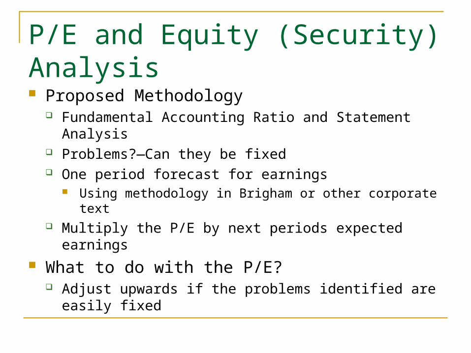
P/E and Equity (Security) Analysis Proposed Methodology
Fundamental Accounting Ratio and Statement Analysis Problems?—Can they be fixed One period forecast for earnings
Using methodology in Brigham or other corporate text Multiply the P/E by next periods expected earnings
What to do with the P/E? Adjust upwards if the problems identified are easily fixed

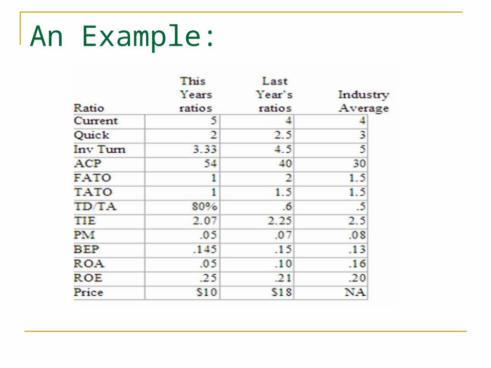
A Simple Valuation Model for Equity A simple model of security analysis: Many corporate finance books discuss
accounting statements in one chapter and long term financial planning in another chapter, while investment and security analysis books do little with these issues in actually arriving at common stock values. Given the difficulty of using econometric models in producing multi-period cash flows—a methodology based on projected accounting statements seems logical. The first step in such an analysis would be to evaluate the accounting ratios from both a time and an industry (benchmark) dimension. If there are problems can they be fixed and how long will it take to fix them—one, two, three, or more years? The next step would be to use a guess about next year's sales and then project next year's earnings incorporating any changes indicated by the ratios. At the same time you would adjust the P/E ratio upwards if problems are fixable. The last step would be to multiply the earnings projection by the P/E ratio (remember this is a present value interest factor) to arrive at an estimate of price. Appendix 1 gives an example of this methodology.
This same methodology can be used for discovering the total value for a company. The only difference is that once the price per share is calculated, simply multiply by the number of shares outstanding to get total equity value. Calculate the present value of the debt using the appropriate interest rates. Adding up the present value of the debt and the price (present value) of the equity will give the total firm value.

An Example:
An Example:

Example:

Example:

Example:

Example

P/E and the ‘Market’ Discount Rate

P/E and the ‘Market’ Discount Rate

P/E(expected) or P/E(current)?

P/E(expected) or P/E(current)?

P/E(expected) or P/E(current)?

What Can We say about the P/E
Looking at the DDM (Gordon Growth model) high P/E’s are associated with relatively low required rates
of return and low P/E’s are associated with relatively high required rates of return, i.e. a negative relationship.
Looking at the individual function arguments we see firstly that increasing (decreasing) the required rate of return, k,
causes the P/E to fall (rise) in all cases where k > g. In all cases, where k > g, part 2 of equation (2) sees smaller
contributions from growth (as k is increased) because of the discounting aspect of part 2 of the equation.
Secondly, increasing (decreasing) ROE causes the P/E to rise (fall). Since the projects have a positive net
present value, increasing growth by raising the ROE adds to the P/E through the growth part of the equation (part 2).
Third increasing (decreasing) b causes the P/E to rise (fall), when you are investing in positive NPV
projects; but the opposite is true when you have negative NPV projects.

Table 1Panel 1—Calculated P/E ratios (Negative NPV) (50% plowback)
Varying the required rate of return
b k ROE P/E1 1st part (2) 2nd part (2)
0.5 5% 2.5% 13.33 20.00 -6.67
0.5 7.5% 2.5% 8.00 13.33 -5.33
0.5 20% 10% 3.33 5.00 -1.67
0.5 40% 10% 1.43 2.50 -1.07
0.5 60% 10% 0.91 1.67 -0.76
0.5 80% 10% 0.67 1.25 -0.58
0.5 100% 10% 0.53 1.00 -0.47
0.5 500% 10% 0.10 0.20 -0.10
0.5 1000% 10% 0.05 0.10 -0.05
0.5 40% 20% 1.67 2.50 -0.83
0.5 60% 20% 1.00 1.67 -0.67
0.5 80% 20% 0.71 1.25 -0.54
0.5 100% 20% 0.56 1.00 -0.44
0.5 500% 20% 0.10 0.20 -0.10
0.5 1000% 20% 0.05 0.10 -0.05
0.5 60% 40% 1.25 1.67 -0.42
0.5 80% 40% 0.83 1.25 -0.42
0.5 100% 40% 0.63 1.00 -0.38
0.5 500% 40% 0.10 0.20 -0.10
0.5 1000% 40% 0.05 0.10 -0.05

Table 1Panel 2—Calculated P/E ratios (Positive NPV) (50% plowback)
Varying the required rate of return Numbers emboldened are when g becomes ? k
b k ROE P/E1 1st part (2) 2nd part (2)
0.5 2% 10% -16.67 50.00 -66.67
0.5 3% 10% -25.00 33.33 -58.33
0.5 4% 10% -50.00 25.00 -75.00
0.5 5% 10% #DIV/0! 20.00 #DIV/0!
0.5 6% 10% 50.00 16.67 33.33
0.5 7% 10% 25.00 14.29 10.71
0.5 8% 10% 16.67 12.50 4.17
0.5 9% 10% 12.50 11.11 1.39
0.5 10% 10% 10.00 10.00 0.00
0.5 10% 20% #DIV/0! 10.00 #DIV/0!
0.5 11% 20% 50.00 9.09 40.91
0.5 12% 20% 25.00 8.33 16.67
0.5 13% 20% 16.67 7.69 8.97
0.5 14% 20% 12.50 7.14 5.36
0.5 15% 20% 10.00 6.67 3.33
0.5 16% 20% 8.33 6.25 2.08
0.5 17% 20% 7.14 5.88 1.26
0.5 18% 20% 6.25 5.56 0.69
0.5 19% 20% 5.56 5.26 0.29
0.5 20% 20% 5.00 5.00 0.00
0.5 21% 30% 8.33 4.76 3.57
0.5 22% 30% 7.14 4.55 2.60
0.5 23% 30% 6.25 4.35 1.90
0.5 24% 30% 5.56 4.17 1.39
0.5 25% 30% 5.00 4.00 1.00
0.5 26% 30% 4.55 3.85 0.70
0.5 27% 30% 4.17 3.70 0.46
0.5 28% 30% 3.85 3.57 0.27
0.5 29% 30% 3.57 3.45 0.12
0.5 30% 30% 3.33 3.33 0

Table 1 Panel 3—Calculated P/E ratios (Zero NPV) (50% plowback)
Varying the required rate of return and return on equity
b k ROE P/E1 1st part (2) 2nd part (2)
0.5 10% 10% 10.00 10.00 0.00
0.5 20% 20% 5.00 5.00 0.00
0.5 30% 30% 3.33 3.33 0.00
0.5 40% 40% 2.50 2.50 0.00
0.5 50% 50% 2.00 2.00 0.00
0.5 60% 60% 1.67 1.67 0.00
0.5 70% 70% 1.43 1.43 0.00
0.5 80% 80% 1.25 1.25 0.00
0.5 90% 90% 1.11 1.11 0.00
0.5 100% 100% 1.00 1.00 0.00

Table 2 Panel 1—Calculated P/E ratios (Negative NPV)
(50% plowback)Varying ROE
b k ROE P/E1 1st part
(2) 2nd part
(2)
0.5 5% 1% 11.11 20.00 -8.89
0.5 5% 2.50% 13.33 20.00 -6.67
0.5 5% 5% 20.00 20.00 0.00
0.5 10% 1% 5.26 10.00 -4.74
0.5 10% 5% 6.67 10.00 -3.33
0.5 10% 10% 10.00 10.00 0.00
0.5 20% 15% 4.00 5.00 -1.00
0.5 20% 20% 5.00 5.00 0.00
0.5 30% 25% 2.86 3.33 -0.48
0.5 30% 30% 3.33 3.33 0.00
0.5 40% 35% 2.22 2.50 -0.28
0.5 40% 40% 2.50 2.50 0.00
0.5 50% 45% 1.82 2.00 -0.18
0.5 50% 50% 2.00 2.00 0.00
0.5 60% 55% 1.54 1.67 -0.13
0.5 60% 60% 1.67 1.67 0.00

Table 2 Panel 2—Calculated P/E ratios (Positive NPV)
(50% plowback)Varying ROE Numbers emboldened are when g becomes close to ? k
b k ROE P/E1 1st part (2) 2nd part (2)
0.5 5% 7.50% 40.00 20 20
0.5 5% 9% 100.00 20 80
0.5 10% 15% 20.00 10 10
0.5 10% 19% 100 10 90
0.5 20% 25% 6.67 5 1.67
0.5 20% 30% 10.00 5 5
0.5 30% 35% 4.00 3.33 0.67
0.5 30% 40% 5.00 3.33 1.67
0.5 40% 45% 2.86 2.50 0.36
0.5 40% 50% 3.33 2.5 0.83
0.5 50% 55% 2.22 2 0.22
0.5 50% 60% 2.50 2 0.5
0.5 60% 65% 1.82 1.67 0.15
0.5 60% 70% 2.00 1.67 0.33

Table 3 Panel 1—Calculated P/E ratios (Negative NPV)
Varying b
b k ROE P/E1 1st part (2) 2nd part (2)
0.0 5% 2.50% 20.00 20.00 0.00
0.5 5% 2.50% 13.33 20.00 -6.67
1.0 5% 2.50% 0.00 20.00 -20.00
0.0 10% 5% 10.00 10.00 0.00
0.5 10% 5% 6.67 10.00 -3.33
1.0 10% 5% 0.00 10.00 -10.00
0.0 20% 15% 5.00 5.00 0.00
0.5 20% 15% 4.00 5.00 -1.00
1.0 20% 15% 0.00 5.00 -5.00
0.0 30% 25% 3.33 3.33 0.00
0.5 30% 25% 2.86 3.33 -0.48
1.0 30% 25% 0.00 3.33 -3.33

Table 3 Panel 2—Calculated P/E ratios
(Positive NPV) Varying b
Numbers emboldened are when g becomes ? k
b k ROE P/E1 1st part (2) 2nd part (2)
0.00 5% 10% 20.00 20.00 0.00
0.25 5% 10% 30.00 20.00 10.00
0.50 5% 10% #DIV/0! 20.00 #DIV/0!
0.75 5% 10% (10.00) 20.00 (30.00)
1.00 5% 10% 0.00 20.00 (20.00)
0.00 15% 20% 6.67 6.67 0.00
0.25 15% 20% 7.50 6.67 0.83
0.50 15% 20% 10.00 6.67 3.33
0.75 15% 20% lg neg num 6.67 lg neg num
1.00 15% 20% 0.00 6.67 (6.67)
0.00 25% 30% 4.00 4.00 0.00
0.25 25% 30% 4.29 4.00 0.29
0.50 25% 30% 5.00 4.00 1.00
0.75 25% 30% 10.00 4.00 6.00
0.85 25% 30% (30.00) 4.00 (34.00)
1.00 25% 30% 0.00 4.00 (4.00)

Table 3 Panel 3—Calculated P/E ratios (Zero NPV) Varying b
Numbers emboldened are when g becomes ? k
b k ROE P/E1 1st part (2) 2nd part (2)
0.00 5% 5% 20.0 20.0 0.0
0.50 5% 5% 20.0 20.0 0.0
1.00 5% 5% 20.0 20.0 0.0
0.00 10% 10% 10.0 10.0 0.0
0.50 10% 10% 10.0 10.0 0.0
1.00 10% 10% #DIV/0! 10.0 #DIV/0!
0.00 25% 25% 4.0 4.0 0.0
0.50 25% 25% 4.0 4.0 0.0
1.00 25% 25% #DIV/0! 4.0 #DIV/0!
0.00 75% 75% 1.3 1.3 0.0
0.50 75% 75% 1.3 1.3 0.0
1.00 75% 75% #DIV/0! 1.3 #DIV/0!

What Can we say about the Future P/E Evidence of Mean Reversion So stay tuned

WHAT DO P/E RATIOS SAY ABOUT COMPANIES?—Early Results Data was collected from Standard and Poor’s Market
Insight for the 10 year period beginning in 1991 for the Dow 30 companies. The ratios selected are: ROI (NET)—Net Return on Average Investment. ROE (NET)—Net Return on Average Equity. ROE (REL)—Relative Net Return on Average Equity. P/E (CLS)—Price Earnings Ratio. P/E (REL) Price Earnings Ratio Relative to the S&P 500.
P/CF (CLS)—Price/Cash Flow—Close. Dividend Yield. . Relative Dividend Yield. Book Value. LTD/EQ—Long-Term Debt to Common Equity.

WHAT DO P/E RATIOS SAY ABOUT COMPANIES?—Early Results Data was collected from Standard and Poor’s Market Insight for
the 10 year period beginning in 1991 for the Dow 30 companies. The ratios selected are: CURR—Current Ratio. QUICK—Quick Ratio. INTCOV—Interest Coverage. TIE—Times Interest Earned. SALES Growth EPS (BASIC)—Growth. Cash Flow--Growth Inventory Turnover. Receivables turnover. Total Assets Turnover. Net Profit Margin.

WHAT DO P/E RATIOS SAY ABOUT COMPANIES?—Early Results The ratios were sorted from low to high and given a score of 1 to
30 (1 is low, 30 is high). Higher ratios are ‘better’. Only the debt ratio is backwards.
The score for each company is the sum of the individual ratio’s ranking score.
Company with the highest score is the ‘best’ while the company with the lowest score is the ‘worst’ performing company.
The data scores were sorted from high to low along with the associated ratio data for 1991. The tri-tiles were then followed for the remaining years to see what happens to the ratios. T-tests are performed on the various years to see if there is a
significant difference in the means. Tables 2a through 4e are presented at the end of this paper.

WHAT DO RATIOS SAY ABOUT COMPANIES? ‘Bad’ companies are associated with low
P/E’s ‘Good’ companies are associated with high
P/E’s ‘Bad’ companies get better and this is
reflected in various ratios as well as the P/E This implies that equity and firm valuation
using a fundamental—P/E approach seems valid.

Conclusion
P/E multiples are adjusted present value factors Thus using them in analysis is theoretically sound
P/E multiples along with fundamental analysis seems to be a reasonable valuation technique
P/E multiples can be used to find the ‘Market’ discount rate
More work needs to be done

Other Approaches to Stock Valuation
Book value per share is the amount per share that would
be received if all the firm’s assets were sold for their exact
book value and if the proceeds remaining after paying all
liabilities were divided among common stockholders.
This method lacks sophistication and its reliance on
historical balance sheet data ignores the firm’s earnings
potential and lacks any true relationship to the firm’s value
in the marketplace.
Book Value

Other Approaches to Stock Valuation Liquidation value per share is the actual amount per share
of common stock to be received if al of the firm’s assets
were sold for their market values, liabilities were paid, and
any remaining funds were divided among common
stockholders.
This measure is more realistic than book value because it
is based on current market values of the firm’s assets.
However, it still fails to consider the earning power of
those assets.
Liquidation Value

Free Cash Flow Model
Stock Valuation Models
The free cash flow model is based on the same premise as the dividend valuation models except that we value the firm’s free cash flows rather than dividends.
Free Cash Flow Model
Stock Valuation Models
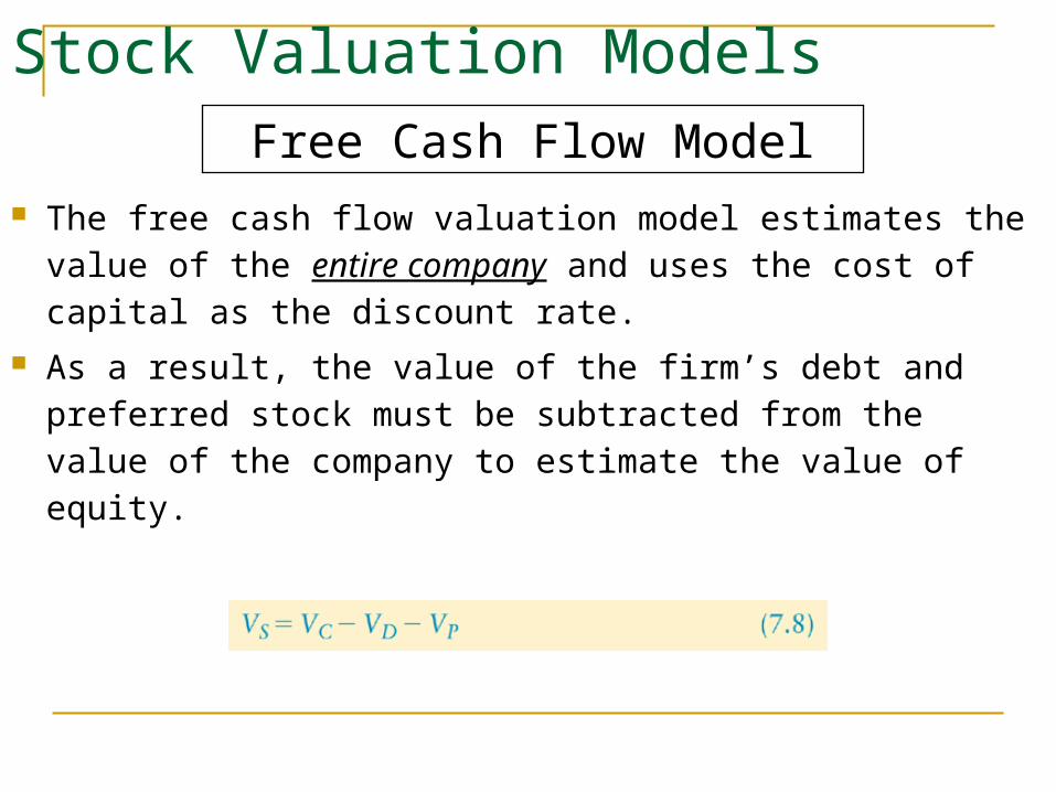
The free cash flow valuation model estimates the value of the entire company and uses the cost of capital as the discount rate.
As a result, the value of the firm’s debt and preferred stock must be subtracted from the value of the company to estimate the value of equity.

Free Cash Flow Model
Stock Valuation Models
Dewhurst Inc. wishes to value its stock using the free cash flow model. To apply the model, the
firm’s CFO developed the data given in Table 7.3.

Free Cash Flow Model
Stock Valuation Models
Step 1: Calculate the present value of the free cash flow occurring from the end of 2009 to infinity, measured at the beginning of 2009.

Free Cash Flow Model
Stock Valuation Models
Total FCF2008 = $600,000 + $10,300,000 = $10,900,000
Step 2: Add the PF of the FCF found in step 1 to the FCF for 2008.
Step 3: Find the sum of the present values of the FCFs for 2004 through 2008 to determine VC. This
is shown in Table 7.4 on the following slide.

Free Cash Flow Model
Stock Valuation Models

Free Cash Flow Model
Stock Valuation Models
VS = $8,628,620 - $3,100,000 = $4,728,620
Step 4: Calculate the value of the common stock using equation 7.6.

PEG

PEG
Actually the real numbers would be 100 times larger


