Pedestrian Detection using a boosted cascade of Histogram ...

Information Coding Group

Department of Electrical Engineering

Pedestrian Detection using a

boosted cascade of Histogram of

Oriented Gradients

Author:

Cristina Ruiz Sancho <[email protected]>

Advisors: Jörgen Ahlberg <[email protected]>

Nenad Markuš <[email protected]>

Philippe Salembier <[email protected]>

Examiner: Robert Forchheimer <[email protected]>

Linköping – Barcelona, August 2014

Abstract

Pedestrian detection has been an active area of research in recent years; its interest relies

on the potential positive impact on quality of life of the related applications (surveillance

systems, automotive safety, robotics, multimedia content analysis, assistive technology and

advanced interactive interfaces, among others).

The large variability of human appearances, poses and context conditions makes

pedestrian detection to be one of the most challenging tasks in computer vision. Although

many significant approaches have been proposed lately, pedestrian detection still offers a

wide framework of improvement, mainly in terms of accuracy and efficiency.

The present thesis aims to study the influence of different training parameters values on

the performance of a pedestrian detector. First, a pedestrian detector, using a boosted

cascade of Histograms of Oriented Gradients, is built from scratch. Afterwards, a sensitivity

analysis is carried out taking into account significant variables, such as the number of training

samples, the feature (HOG) or classifier (SVM) parameters, the feature selection technique,

the negatives resampling treatment and the typology of the employed weak classifier.

Contents

1. Introduction............................................................................................................................... 1

2. Background Theory ................................................................................................................... 3

2.1. Object Detection ................................................................................................................ 3

2.2. Feature Extraction .............................................................................................................. 4

2.2.1. Intensity-based Features ............................................................................................. 4

2.2.2. Texture-based Features .............................................................................................. 6

2.2.3. Shape-based Features ................................................................................................. 6

2.2.4. Histograms of Oriented Gradients (HOGs) .................................................................. 7

2.3. Classification Techniques ................................................................................................. 10

2.3.1. Support Vector Machines .......................................................................................... 11

2.3.2. Decision Trees ........................................................................................................... 12

2.3.3. Ensemble Methods.................................................................................................... 13

2.4. Pedestrian Detection (State of the Art) ........................................................................... 19

3. Implementation ....................................................................................................................... 21

3.1. Image Dataset .................................................................................................................. 21

3.2. Overall Architecture Design ............................................................................................. 23

3.2.1. Learning stage ........................................................................................................... 23

3.2.2. Runtime stage ........................................................................................................... 26

3.3. Overall System Development ........................................................................................... 28

3.3.1. Development environment ....................................................................................... 28

3.3.2. Code structure ........................................................................................................... 29

4. Results ..................................................................................................................................... 34

4.1. Baseline detector ............................................................................................................. 34

4.1.1. Parameters configuration ......................................................................................... 34

4.1.2. Learning results ......................................................................................................... 35

4.1.3. Runtime results ......................................................................................................... 37

4.2. Sensitivity analysis ............................................................................................................ 40

4.2.1. Feature blocks geometry ........................................................................................... 40

4.2.2. Histogram of Oriented Gradients computation ........................................................ 41

4.2.3. SVM soft margin ........................................................................................................ 43

4.2.4. Number of training samples ...................................................................................... 44

4.2.5. Feature selection subset dimension ......................................................................... 45

4.2.6. Negatives resampling technique ............................................................................... 46

4.2.7. Typology of weak classifier........................................................................................ 47

5. Conclusions.............................................................................................................................. 48

5.1. Technical conclusions ....................................................................................................... 48

5.2. Future work ...................................................................................................................... 49

Appendices .................................................................................................................................. 51

A. Data flowcharts ................................................................................................................... 51

List of Figures .............................................................................................................................. 55

List of Tables ................................................................................................................................ 57

References ................................................................................................................................... 58

Pedestrian Detection using a boosted cascade of Histogram of Oriented Gradients

- 1 -

1. Introduction

Computers have become indispensable in our everyday life; they are useful in many areas

because they can do specific and complex tasks in a more efficient and accurate way than

humans. However, they are still not able to perform efficiently some intelligent high-level

tasks, such as analysis of scenes, speech recognition, reasoning and logical interpretation, that

humans perform subconsciously and naturally a lot of times every day.

Developing vision systems that perform human cognitive capabilities is one of the edge areas

of current research. Object recognition is one of these abilities; at a simple glance a human

can categorize an object effortlessly and instantaneously. Besides, humans are able to identify

objects, such as cars or people, despite of their variation in color, pose, texture, deformation,

occlusions, illumination and background complexity. Many researchers working in computer

vision are focused on developing object recognition systems that are able to tell the specific

identity of an object being observed. One of the primary tasks to achieve that goal is the

implementation of accurate object detection, which means localizing, in terms of position and

scale, a specific object in a static image. Pedestrian detection is a particular case of object

detection where the target object class is people. It has been an active area of research

recently because many applications involve people’ location and movement tracking and, what

is more, because of the potential positive impact of these derived applications, such as

surveillance systems, automotive safety, robotics, multimedia content analysis, assistive

technology and advanced interactive interfaces.

Although many approaches have already been proposed, pedestrian detection is still a

challenging task due to the wide variability of pedestrian appearances. Furthermore, it is also a

competitive domain since the high research activity in the field continuously pushes the upper

boundary of accuracy and efficiency to new levels. Existing pedestrian detection methods use

combinations of basic features and trainable classifiers (SVM, boosted classifiers or random

forests).

The purpose of the present thesis is to develop and evaluate a state of the art pedestrian

detection approach. In particular, the work will pursue two differentiate goals:

Building a pedestrian detector from scratch and evaluate its performance, both in

terms of accuracy and speed. A pedestrian detection can be understood as a

combination of two building blocks, a feature extraction algorithm and a classification

method that uses the features to make the object/non-object decision. Our approach

uses a boosted cascade of Histograms of Oriented Gradients as features and Support

Vector Machines as classifiers.

Carry out a sensitivity analysis in order to study how the training parameters influence

the learning process development and the final performance of the pedestrian

detector.


- 2 -

The work proposal should help to, first, get familiar with the classification problem and

machine learning techniques in general, and, then, acquire deeper knowledge about

pedestrian detection task. Besides, it should allow to face the common dilemmas of pedestrian

detection implementation and to observe the difficulties of the learning process. Finally, it

should be useful to study and evaluate the particular behaviour of our approach, in terms of

learning development and performance, to draw useful conclusions to suggest new future

lines of work.

This chapter introduces the topic of pedestrian detection and explains the main motivation

and goals of the present thesis work. The rest of the document is organized as follows:

Chapter 2. Background theory, describes the state of art in object detection, focusing

on pedestrian detection. It first introduces some general background theory about

image classification and explains the most remarkable existent features and classifiers

used for object detection purposes. Then, it provides an overview of the pedestrian

detection research approaches.

Chapter 3. Implementation, presents our pedestrian detection approach. First,

describes the overall detection framework design and, after, gives the implementation

and code structure details.

Chapter 4. Results, exposes the obtained pedestrian detector structure and

performance, and proposes the sensitivity analysis, explaining all the evaluated

configurations and the key experimental observed results.

Chapter 5. Conclusions, summarises the extracted results providing a discussion of the

main conclusions and a suggestion of directions for future work improvements.


- 3 -

2. Background Theory

2.1. Object Detection

Object detection [1] is a computer technology that aims to detect and localize (find) objects of

a certain predefined category (class) in static digital images or video frames.

The following are some basic concepts of image processing related with object detection that

are important to be clarified to avoid further confusion (given examples assume people as the

object class of interest) [2]:

Object-presence detection: determining if one or more instances of a particular object

class are present in an image, at any location or scale. – Does the image contain people?

Object detection / Object localization: determining the specific location and scale of one

or more instances of a particular object class in an image. – Where are the people (if

any) in the image?

Object recognition: determining the identity of each detected instance of a particular

object class in an image. – Is Peter the person in the image (if any)?

Object categorization: determining the object class that corresponds to every instance

present in an image. – This is a person, this is a table, and this is a car.

Object detection systems are usually composed by two major procedures that we analyze

separately in this work: feature extraction and classification. The feature extraction step

encodes the visual appearance of the image in predefined features, whereas the classification

step determines, using the previous extracted features and a particular classifier, if a region

contains the object of interest or not.

Figure 2.1 Object detection general structure.

The present thesis is focused in pedestrian detection, a particular case of object detection

where human body is the class of interest. Therefore, the goal of pedestrian detection is to

find all instances of human beings present in an image. This technology has applications in

many areas of computer vision including surveillance, automotive safety and robotics.


- 4 -

2.2. Feature Extraction

A feature is an individual attribute or property of an object that is relevant in describing and

recognizing it and that allows distinguishing it from other objects.

Feature extraction [3] is the process of transforming a given set of input data (usually

redundant and large) into a reduced representation which is known as set of features (feature

vector = grouped features of a given data).

Feature extraction and representation, which also involves previous steps of feature selection

and detection, is used as starting point in many computer vision algorithms. Feature selection

[4] means choosing discriminating features to find the best possible data representation.

Feature selection is key to every machine learning and classification algorithm since it

conditions directly its performance. It should take into account not only relevance of the

features, but also other aspects such as volume data reduction. The size of the feature set

concerns computational efficiency and algorithm speed, complexity and accuracy.

Therefore, efficient and effective feature selection and extraction is a crucial step for image

analysis and, especially, for object detection and recognition. In this particular case, the input

data is an image and the most common features to extract are visual descriptors mainly based

on color, texture or shape [5].

According to its complexity, image features can be classified as low-level features, which are

basic features that can be extracted directly from the image pixel information, and high-level

features, which require previous processing steps and are usually based on low-level features.

What is more, [6] image features can also be classified as global features, which are obtained

from the entire image region and a single vector describes the image as a whole, or local

features, which consider and represent only a small area of the image region. Global features

are much more sensitive to variability in terms of object appearance (pose, occlusion and

illumination conditions) than local features.

2.2.1. Intensity-based Features

Intensity features are based directly on absolute pixel values from either color or grayscale

images. Intensity is a low-level and scale-invariant feature that is essential for image

characterization; it is widely used as a feature due to its perceptual relevance and its simplicity.

However, grayscale or color intensity alone does not provide a complete image description,

especially, because it lacks structural information. Besides, in general, working with image

intensities, as they are pixel level attributes, makes feature calculation computationally

expensive.

Pixel intensity comparison [7] [8] is the simplest intensity-based feature which consists in

comparing two pixel intensity values. The output is a single number per comparison, it is

possible to compare every pair of pixels in an image, but typically, to reduce feature

dimension, only a few set of them are evaluated.


- 5 -

{ ( ) ( )

} (2.1)

Pixel intensity difference is a derived feature that consists in computing the difference

between two pixel intensity values. In this case, the feature output can be the pixel difference

value itself or also a binary number assigned according to an established threshold.

( ) ( ) (2.2)

{ ( ) ( )

} (2.3)

Average intensity is another simple feature that merely measures the mean intensity at a

specific sub region of the image.

Color-based features refer to color images and should be defined according to a particular

color space, such as RGB, LUV, CIE Lab or HSV. The main color features proposed in the

literature are color histogram [9] [10], color moments (CM) [11], color coherence vector (CVV)

[12]and color correlogram [13].

Grayscale-based features refer to features extracted from gray images, where every pixel has

only one value from 0 to 255 that represents gray intensity. The highlight among grayscale-

based features is the use of the Haar wavelet, a sequence of functions with a natural

mathematical structure for describing patterns. Haar wavelet features [14] [15] exploit the

idea of using a complete set of basic functions, wavelet coefficients, to represent the structure

of an object. They describe the oriented contrasts present in an image by collecting local

intensity differences between adjacent regions. Haar wavelet has been the inspiration for

other widely used features such as Haar-like features [16] [17], a generalization using arbitrary

feature dimensions and different orientations. Every Haar-like feature consists of black and

white rectangular regions placed at specific locations in the image. The black and white regions

should have the same size and shape and must be horizontally or vertically adjacent.

Figure 2.2 A set of extended Haar like features [18]; a) edge features, b) horizontal and vertical line features, c) diagonal line features and d) center-surround features and special diagonal features.


- 6 -

The value of the feature is computed by the difference between black and white image areas,

in other words, the sum of the pixel intensity values within the white rectangles are subtracted

from the sum of pixel intensity values in the black rectangles.

∑ ∑

(2.4)

In comparison with raw pixel-based features, Haar-like features can reduce the intra-class

variability (and increase the inter-class variability) making classification easier and less

computationally expensive.

2.2.2. Texture-based Features

Texture features aim to describe the local density variability and patterns inside the surface of

an object. Unlike color, which is usually a pixel property, texture can only be considered from a

group of pixels. In general, texture features have strong discriminative capability but also high

computational complexity. Texture feature extraction techniques can be classified into spatial

methods, which extract features directly in the original image domain by computing pixel

statistics, and spectral methods, which compute features in the transformed image frequency

domain. Spatial methods are easy to understand because of their semantic meaning and are

suitable for irregular shapes, but are sensitive to noise and distortions. Spectral methods lack

from semantic information and can only be applied to square regions, but they are robust and

usually less computational.

Most well-known spatial texture features, such as the basic Haralick features [19], derived

from Grey-level co-occurrence matrix (GLCM) [20] and spectral texture features mainly adopt

Gabor filters [21] implementation approaches. Local Binary Pattern (LBP) [22] which codifies

local primitives (edges, spots, flat areas) into a feature histogram, is the main texture

descriptor used in pedestrian detection.

2.2.3. Shape-based Features

Shape features encode the size and geometrical form of the objects. Shape feature extraction

techniques can be classified into contour based methods, which compute features only from

the object boundary information, or region based methods, which extract features from the

entire object area. Contour based techniques tend to be more sensitive to noise as they only

use a part of the entire object information (edges).

Contour based methods usually employ edge detectors to extract low level features. At the

same time, most edge detectors rely on gradient computation; therefore, gradient-based

features are considered a specific type of shape-based features. The gradient can be a feature

itself, or just the base to compute higher-level features. Common gradient-based features are

Edge Orientation Histograms (EOH) [23] [24] and Histogram of Oriented Gradients (HOG)

[25]. Both features describe the spatial gradient orientations in an image; meanwhile EOH

consist on defining the relation between two specific orientations in an image region, HOG

consist on counting the occurrences of a set of orientations in image blocks. EOH is invariant to


- 7 -

global illumination changes, and HOG is not only invariant to photometric but also to

geometric transformations, except for object rotation. Later variants from HOG are Pyramid

Histogram of Oriented Gradients (PHOG) [26] [27] with the objective to take the spatial

property of the local shape into account, and Domination Orientation Templates (DOT) [28]

which instead of computing complete histograms only considers the most dominant

orientations. Scale Invariant Feature Transform (SIFT) [29] is a gradient-based shape

descriptor widely-used for object recognition purposes, SIFT is remarkable because of its

invariability to scale and rotation and its robustness to noise, illumination changes and affine

distortions.

In addition, Chamfer matching [30] and Shape Context [31] are also popular shape descriptors

used in object recognition; they are based on matching object shapes to reference image

structures. A mathematical distance, such as chamfer or Euclidean, determines the similarity

between the two compared objects. Chamfer matching is a global approach, trying to match

complete silhouettes; meanwhile Shape Context is local and works matching particular and

relative point locations on a shape.

Moreover, shapelets [32] and edgelets [33] have been proposed recently as shape gradient-

based features specifically for pedestrian detection.

2.2.4. Histograms of Oriented Gradients (HOGs)

The Histogram of Oriented Gradient (HOG) is a feature that describes the distribution of the

spatial directions in every image region. It exploits the thought that local object appearance

can be characterized quite well by the distribution of local intensity gradients or edge

directions. The basic idea is to divide an image into small spatial regions and, for each region,

create a 1-D gradient orientation histogram with the gradient direction (histogram bin

selection) and gradient magnitude (histogram bin weight/contribution) information from all

the pixels in the region. Those histograms are contrast-normalized using block-wise pattern

and concatenated in order to obtain the final visual descriptor.

The detailed algorithm implementation is done as follows:

Gamma/Color normalization: Image pre-processing step to ensure normalized color

and gamma values. This step can usually be omitted because has only a little effect on

performance.

Gradient computation: The first step is to compute the image horizontal

( ( )) and vertical gradients ( ( )), which is usually done by filtering. It is

verified that the simple 1-D centered filtering masks, [-1, 0, 1] and [-1, 0, 1]T, with no

smoothing, perform the best.


- 8 -

Figure 2.3 Original pedestrian image, horizontal ( ) and vertical ( ) gradient images.

With the horizontal and vertical gradient information, we can compute the gradient

orientation and magnitude for each pixel in the image.

( ) √ ( ) ( )

(2.5)

( ) ( ( )

( )) (2.6)

Figure 2.4 Gradient magnitude (m) and orientation (θ).

For color images, the gradients are computed separately for each color channel and,

for each pixel, it is chosen the channel with the highest gradient magnitude.

Spatial / Orientation binning: HOG extraction is a single window approach, the image is

divided into regions called blocks and, at the same time, each block is divided into

smaller regions called cells. One histogram per cell is extracted and, concatenating

them, one normalized descriptor (X-D vector) per block. Overlapping between blocks is

introduced to ensure consistency across the whole image reducing the influence of

local variations. Cells can be rectangular (R-HOG) or circular (C-HOG).


- 9 -

Every histogram has the same certain number of bins, which determines its precision.

The bins represent the gradient orientations (angles) and must be equally spaced over

0˚-180˚ (unsigned gradients) or 0˚-360˚ (signed gradients). One histogram per cell is

computed; each pixel in the cell contributes to the histogram adding its magnitude

value to its corresponding orientation bin, this weighting value is called vote. The vote

can be function of the magnitude, but it is proved that using directly the magnitude

value itself produces the best results. If necessary, the votes can also be interpolated

bilinearly between different neighbor bins.

Figure 2.5 Original image and the correspondent Histograms of Oriented Gradients.

Normalization: Effective local contrast normalization is essential to solve illumination

and foreground-background variations; it is applied at a block level and different

schemes can be used.

Concatenation: The final descriptor is a 1-D vector resultant of concatenating the normalized histograms from every block in the detection window/image.

Figure 2.6 Computation of Histograms of Oriented Gradients

0 40 80 120 160

0 40 80 120 160

0 40 80 120 160

0 40 80 120 160

cell0

cell1

cell2

cell3

Feature vector

{Nº cells/Block x Bins/Histogram}

<4,6,5,4,5,7,1,4,3,

3,5,2,4,5,6,2,7,3,

7,6,2,4,7,6,2,3,4,

3,2,4,6,5,3,2,5,7>


- 10 -

2.3. Classification Techniques

Classification [34] is the process in which individual elements are grouped according to the

similarity between the element and the description of the group. In other words, classification

consists in attributing a predefined category or class label to a certain instance of an input

dataset, separating, therefore, the input data into different categories (classes) with common

features. Although the input data can have many different origins theoretically, in practice it is

treated usually as a simple vector of numbers.

In general, classification is a two-step process:

Learning / Training stage - Model construction: given a set of data samples (training

dataset) with examples of the different classes, the goal is to find a model, based on

the extracted dataset features, that explains the target class concept. The resultant

classification model, which is mainly a mathematical function, assigns each input data

sample to a certain predefined category (class).

A classification technique or classifier is the systematic approach to building

classification models from an input dataset. Each classifier employs a learning

algorithm to identify the model that best fits in the specific dataset. Machine learning

algorithms are focused on finding data relationships and analyzing the procedures for

extracting such relations. In a particular training dataset, every sample is represented

by the same set of features. If the samples are class labelled then the learning method

is called supervised, however, if the samples are given with no class labels then the

learning is called unsupervised. In the present work we focus in supervised machine

learning techniques [35].

Testing / Running stage - Model usage: the classification model or classifier, obtained

in the previous step, should be able to classify future or new unknown instances. But

first, its performance is often proved using a set of already labelled data (testing

dataset).

Image classification, in particular, consists in categorizing all pixels or regions in a digital image

into one of the possible classes, and then, being able to determine if the image contains or not

a particular object. Pedestrian detection is a particular case of image binary classification,

where the samples (x) are images and the class labels can only be 1 if the image contains a

pedestrian (positives), or 0 or -1, if not (negatives). The most common classification

methods/classifiers used in pedestrian detection are presented in the following subsections.

Classification

model

Feature vector

(v)

Class label

(y)

Sample

(x)

Figure 2.7 Classification as the task of mapping an input instance x, with an attribute set v, into its class label y.


- 11 -

2.3.1. Support Vector Machines

Support Vector Machine [36] introduced by Vapnik in 1995 [37], is a traditional supervised

machine learning technique used for classification (regression, and other tasks) which aims to

optimize a hyperplane as the decision function to separate two data classes, positive and

negative samples. The classification with less error is achieved by the hyperplane that

maximizes the margin, which means creating the largest possible distance between the

separating hyperplane and the nearest instances on either side of it.

It is not always possible to find a hyperplane that exactly separates all the samples in a

particular given dataset. This problem can be solved by using a soft margin that accepts a

certain level of misclassification.

SVMs are used to classify linearly separable data, but they can also efficiently perform a non-

linear classification mapping the classification problem into a higher dimensional space. The

idea is to transform the original non-linearly separable data to a new high-dimensional space,

called the feature space, where it becomes linearly separable and where it is possible to

construct the separating hyperplane. The non-linear classification is done using kernels, which

are special functions that allow calculating inner products directly in the feature space,

without need to perform the mapping precisely and making the problem computation feasible.

The good performance of SVMs has been proven in many fields (bioinformatics, text, image

recognition…) and their complexity is not affected by the number of features of the training

data. Therefore, SVMs are adequate to use especially when the number of features is large

with respect to the number of samples of an specific learning dataset.

V2

V1

h1

h2 margin 1

margin 1

margin 2

margin 2

Figure 2.8 Two-dimension linear SVM representation; choosing the hyperplane that maximizes the margin (h1).


- 12 -

2.3.2. Decision Trees

A decision tree, chapter 4 in [34], is a simple but very popular and comprehensible

classification technique. It consists of a hierarchical structure built with nodes and edges

(branches) that classifies samples by sorting them according to node decisions. Each node

represents a sample attribute (feature) test condition, and each branch represents a value that

the sample attribute can undertake.

In every tree there exist three different types of nodes:

Root node: it is the starting point; it has no incoming branches but one or more

outgoing branches.

Internal nodes: they conform the body of the tree, each of them has exactly one

incoming branch and two (binary tree) or more outgoing branches.

Terminal node or “leaf”: it represents the final classification decision; each leaf node is

assigned to a certain class label. Each of them has exactly one incoming branch and no

outgoing branches.

Classification starts from the root node, the root node condition is tested to the sample to be

classified and, based on the test result, the appropriate branch is followed. The branch leads to

a new internal node with another condition to test. This procedure is applied sequentially,

creating a downward path in the tree, until a leaf node is reached. The class label associated to

the reached leaf node is assigned to the sample.

Root node

Internal node

Leaf node (assigned to class y1)

Leaf node (assigned to class y2)

y1

f1 f1(v) ≥ t1 f1(v) < t1

{x, v}

f2 f3

f4

f3(v) ≥ t3 f2(v) ≥ t2

f4(v) ≥ t4

f2(v) < t2

f4(v) < t4

f3(v) < t3

y2

y2 y1

y1

Figure 2.9 Binary decision tree with binary classification (classes y1 and y2). Where x is the sample to be classified, v is the feature vector associated to the sample, fn are the attribute test conditions (split functions) and tn the thresholds in each n node conditions.


- 13 -

How to learn/built a decision tree?

Given a dataset of training samples (xi), each of them annotated with a vector of features (vi),

and a class label (yi), exponentially many different decision trees can be constructed. The goal

is to find the optimal tree (or the most accurate tree possible to learn in a reasonable period of

time) which means finding the optimal structure of attribute test conditions. Usually, the tree

is grown in a recursive way using induction algorithms, such as Hunt’s algorithm [38] [39] and

CART [40], which employ greedy strategies.

Starting from the root node, each recursive step of the tree-growing process must select the

attribute test condition (splitting function) that best divides the sample dataset at this point.

There are many measures that can be used to determine the best way to split the training

dataset. The most common ones are based on the degree of impurity of the child nodes in

comparison to the parent node; such as entropy criterion, gini or classification error. The larger

the computed difference the better the splitting condition.

( ) ∑

( | ) ( | )

(2.7)

( ) ∑[ ( | )]

(2.8)

( ) [ ( | )] (2.9)

Where is the number of classes, ( | ) is the fraction of samples belonging to class at a

given node .

A specific terminating condition is also needed to stop the tree-growing process. It is possible

to expand the tree until all the training samples in a node belong to the same class; it is also

common to limit the depth of the tree to a maximum number of levels or to determine the

minimum classification accuracy rate accepted.

Decision trees are widely used as basis of more complex techniques, called ensemble

methods, which are constructed combining more than one decision tree. The most popular

ensemble algorithms are bagging, random forests and boosting.

2.3.3. Ensemble Methods

Ensemble methods built a classification model by combining the results of a group of simpler

base models. The performance of an ensemble model is usually better than the performance

of the individuals because it takes advantage of all their different strengths.


- 14 -

a) Bagging

Bagging [41]is an ensemble method that combines many unbiased classification models, each

of which has been built using a different subset of samples from the training dataset. The

individual models or classifiers are, habitually, decision trees. Given a training set of samples,

bagging selects randomly a subset of samples to grow every single tree.

The final prediction of a simple sample

Regression: ( ) ̂ ( )

∑ ( )

Classification: ( ) { ( )} ;

where ( ) is the class assigned to the sample x after testing the kt

random-forest tree.

1. For k=1 to K:

a) Choose randomly, with replacement, a subset Sk = {(x1, v1, y1)… (xM, vM, yM) }

of M training samples from the total dataset S.

b) Train a decision tree 𝐶𝑘.

2. Output the ensemble of trees 𝐶𝑏𝑎𝑔 {𝑐𝑡} 𝐾

Figure 2.10 Pseudo-code of the bagging ensemble algorithm.

Figure 2.11 Bagging ensemble binary classifier (classes y1 and y2) of K decision binary trees. Where Sk are the different subsets of training samples,x is the sample to be classified, v is the feature vector associated to the sample, fn,k are the attribute test conditions (split functions) and tn the thresholds in each n node and k tree.

f3,1(v) ≥ t3,1 f2,1(v) ≥ t2,1

f4,1(v) ≥ t4,1

f2,1(v) < t2,1

f4,1(v) < t4,1

y1

y1

f4,1

f1,1 f1,1(v) ≥ t1,1 f1,1(v) < t1,1

Tree c1, S1

f2,1 f3,1

y2

y2

y1

f3,1(v) < t3,1

…

f3,K(v) ≥ t3,K f3,K(v) < t3,K f2,K(v) ≥ t2,K

f1,K f1,K(v) ≥ t1,K f1,K(v) < t1,K

SK, Tree cK

f2,K f3,

K f2,K(v) < t2,K

y2 f4,K(v) ≥ t4,K f4,K(v) < t4,K

y1

f4,K

y2

y1 y2

c1(x) cK (x)

Dataset S

{x, v, y?}

y = majority vote {ck(x)}1K


- 15 -

Bagging is useful for reducing the variance, which is inversely proportional to the number of

trees in the ensemble. It is possible to find an optimal number of trees in the ensemble to

achieve the desired variance or test error. However, the bias is never modified since every tree

is identically distributed.

b) Random Forests

Random forests [42] [43] are powerful ensemble classifiers resultant of averaging many

random decision trees together. Every random decision tree is grown in a distributed way and

should be uncorrelated with the others. The main difference with bagging is that random

forests introduce randomness not only when selecting every subset of training samples but

also when selecting the features that must be used in each of the decision nodes of the trees.

Figure 2.12 Pseudo-code of the random forest algorithm


Regression: ( ) ̂ ( )

∑ ( )

Classification: ( ) { ( )} ;

where ( ) is the class assigned to the sample x after testing the ck

random-forest tree.

The general error rate of a random forest depends on the strength (low error) of the individual

trees and on the correlation between them. The more decorrelated and the stronger the

individual trees are; the lower error rate the random forest presents.

The number of random features evaluated per node (N) remains constant during the forest

growing and is the only adjustable parameter to which random forests are sensitive. Reducing

M reduces both correlation and strength; so, there exists a trade-off and a challenge to find its

optimal range.

1. For k = 1 to K:

a) Choose randomly a subset Sk = {(x1, v1, y1)… (xN, vN, yN) } of N training

samples from the total dataset S. These samples will be the training set for

growing the current tree.

b) Grow a random decision tree ck, by recursively repeating the following steps

for each terminal node (n) of the tree, until the stop condition is reached.

i. Select N features at random from all input possible features (v) and

create N feature conditions (f).

ii. Pick the best feature condition (fn,k) among the N.

iii. Split the node into two child nodes based on possible values of its

feature condition.

2. Output the ensemble of trees { } .


- 16 -

c) Boosting

Boosting [44] [45] refers to a general learning method of producing a very accurate prediction

rule by combining simple and moderately inaccurate single rules. It is based on the observation

that finding many suitable simple rules is much easier than finding a single highly accurate rule.

The idea is to ensemble a group of single classifiers, called weak classifiers, to create a higher

accurate global classifier, called strong classifier. Therefore, the accuracy of the strong

classifier is better than every single isolated classifier.

The boosting algorithm tracks its own performance to concentrate on misclassified training

samples. In every iteration, one new weak classifier is learned and the samples are weighted in

a way as to focus on the ones that have not been correctly classified by previous rounds. Every

weak classifier brings new insights to the strong classifier as all weak classifiers should

complement each other in an optimal way. After certain number of iterations, the strong

classifier is created by weighting the weak classifiers proportionally to their separately

accuracy performance on the training set.

(2.10)

where is the strong classifier, are the weak classifiers and the associated

contribution.

There exist many boosting algorithms which differ mainly in the method of weighting the

training samples and the weak classifiers they use.

AdaBoost (Adaptive Boosting), proposed in 1995 by Yoav Freund and Robert Shapire [46] [47],

is a practical version of the boosting approach. Unlike the original boosting algorithms,

recursive majority gate formulation (Robert Shapire) and boost by majority (Yoav Freund), the

AdaBoost algorithm is adaptive and does not require prior knowledge of the weak classifiers

accuracy.

The AdaBoost algorithm takes as input a set of M training samples labelled as negatives (-1/0)

or positives (1): {(x1,y1) … ( M,yM)} where yi is the label of a certain instance xi. Then, a group

of N classifiers is tested in the set of samples and the best classifier, according to an error

criterion, from the set is chosen. Usually, the exponential error loss measure is used: eβ if the

classifier fails, and e-β if the classifier succeeds (β> 0). Finally, the algorithm computes the

parameter α, associated with the chosen weak classifier, which measures the importance of

the weak classifier contribution to the final strong classifier. The process is repeated T times,

extracting a new weak classifier per iteration. At the beginning, the samples are initialized with

the same weight, but as the algorithm progresses the weights are modified. The misclassified

samples weights are increased and the correctly classified ones are decreased.


- 17 -


( ) { ∑ ( )

∑

} (2.11)

The AdaBoost pseudocode in Figure 2.13¡Error! No se encuentra el origen de la referencia. is

he most basic and general one, it is also possible to introduce feature selection by training in

every iteration more than one weak classifier and picking the one with lowest error [48].

d) Cascade

Cascading is a particular case of ensemble learning; a cascade classifier consists of stages or

levels, where each stage is usually an ensemble of simple classifiers.

In the cascade, a positive result from the first stage sends the sample to be evaluated of a

second stage. A positive result from the second stage triggers a third stage, and sequentially so

on. However, a negative result at any point leads to the direct rejection of the sample.

The dataset used at each level of the cascade is usually extended by inserting new samples

that replace the ones that have been already rejected. Simpler classifiers are used in the first

stages to reject the majority of negatives before more complex classifiers are used to allow

achieving the desired accuracy. The overall false positive rate and true positive rate of the

cascade are and , respectively, where f is the false positive rate per stage, d is the true

positive rate per stage and L the number of total stages. Hence, there exists a clear accuracy

trade-off as adding more stages to the cascade reduces the false positive rate, but also reduces

the overall true positive rate.

Input: Sequence of M labelled samples {(x1, y1) … (xM, yM)}

Distribution D over the M samples.

Weak learning algorithm – weak classifier c

1. Initialize the weights: ( ) for i = 1 … M.

2. For k = 1 to K:

a) Normalize the weights:

∑

;

b) Train a weak classifier with the calculated weighted samples.

c) Calculate the error of the weak classifier: ∑ | ( ) | ;

d) Set

( ) and

e) Update the weights: | ( ) |

3. Output the strong classifier ∑

Figure 2.13 Pseudo-code of the adaptive boosting algorithm – Adaboost.


- 18 -

Figure 2.14 Cascade of binary classifiers structure.

{ f1, d1 }

Cascade LEVEL 2

Cascade LEVEL L

Cascade LEVEL 1 NEG

NEG

POS

NEG

POS

{ f2, d2 }

Negative

sample.

END

Negative

sample.

Negative

sample.

Positive sample.

{ fL, dL }

POS

{ FPR = fL , TPR = dL }

x


- 19 -

2.4. Pedestrian Detection (State of the Art)

Pedestrian detection has been an active field of research recently; numerous researchers have

reported significant results in this area. However, pedestrian detection is still a challenging task

due to the wide variety of appearances (body pose, occlusions, clothing, lighting, background)

that pedestrians can take in images.

The variability of employed techniques for pedestrian detection purposes is very diverse. In

general, proposed training methods can be classified into holistic approaches, which try to

identify the full-human body using a single detection region, and part-based approaches in

which each part of the body is identified separately and a human is detected if some or all

parts are presented in a reasonable spatial configuration. Additionally, according to the testing

procedure, we can distinguish between sliding window approaches, which densely scan the

image at different positions and scales, and key point approaches, which first extract local

interest points from the image, and then evaluate only regions around these points. At the

same time, several types of features, ranging from low level features to complex visual

descriptors, have been used in combination with different types of classifiers. There is

extensive literature on pedestrian detection techniques and their performance; there even

exist specific detailed surveys that concentrate the state of the art in pedestrian detection [49]

[50].

One of the earliest detectors, proposed by Papageorgiou and Poggio [14], was a sliding

window approach that used multi-scale Haar wavelets and support vector machines (SVM).

Viola and Jones [16] developed these ideas to build a detector that integrated Haar-like

features in a cascade of AdaBoost classifiers. Moreover, they pioneered the use of integral

images for fast feature computation. These contributions continue today to be the basis of

modern detection techniques.

Adoption of features based on gradient information brought important performance gains.

Histogram of oriented gradients (HOG) is the most popular gradient-based feature; it was

introduced in conjunction with SVMs by Dalal and Triggs [25]. At cost of computation time, the

algorithm offers high robustness and accuracy even in complex image environments. In [51]

Zhu et al. improved the algorithm speed by using integral histograms [52]. A similar gradient-

based feature, edge orientation histograms (EOH), was presented by Shashua et al. [53] in

combination again with SVMs.

Shape and texture are other visual common exploited features. Gavrila and Philomin [54] [55]

tested different template matching techniques to detect people. Mori et al [56] modelled

human body configurations represented by local Shape Context. Furthermore, specific shape

features, such as edgelets [33] and shapelets [32], have also been developed and learnt using

boosting algorithms.

Advanced features and new gains appear when introducing motion information. Some of the

approaches that include motion features are [57], that builds a detector for static-camera

using Haar wavelets and a cascade boosting scheme, or [58] that creates new descriptors


- 20 -

called Histograms of Flow, designed for situations with a moving background or camera. All in

all, taking advantage of motion information improves detection performance and reliability for

practical applications.

Although some of the previous low-level features showed considerable good results, they are

often not enough to describe accurately all visual information. A step beyond is done by

combining different simple features, each additional feature provides complementary

information and the overall performance is reasonably improved. Mao et al [59] developed a

system to improve contour detection based on edgelets, Haar-like features and Viola’s

Adaboost cascade framework. Likewise, Wu and Nevatia [60] combined HOG, edgelets and

covariance features. Wang et al [61] combined a texture descriptor based on local binary

patterns (LBP) with HOG features. Wojek and Schiele [62] combined Haar-like features,

shapelets, shape context and HOG features outperforming any individual features.

Part-based methods appear to overcome holistic representation methods limitations in spatial

occlusion situations. Mohan et al. [63] divide human body into four parts: head-shoulder, legs,

left arm and right arm; and learns a part-based detector for each using SVM classifiers and

Haar wavelet features. Shashua et al [53] decomposes pedestrian shape into nine parts, and

uses features of orientation histograms; Mikolajczyk et al [64] uses seven parts (face/head for

frontal view, face/head for profile view, head-shoulder for frontal and rear view, head-should

for profile view and legs) based on local gradient features and follows the Viola&Jones learning

approach. The three part-based detectors outperform their correspondent holistic method.

To sum up, while the used set of features and descriptors is quite diverse, the applied learning

techniques tend to be discriminant classifiers such as AdaBoost or SVMs. According to

different sources [62], HOG and dense Shape Context features perform better than other

features independently of the employed classifier. What is more, a combination of multiple

features tends to improve considerably the overall performance of individual detectors, and

adopting a part-based solution seems to be the most reasonable option.


- 21 -

3. Implementation

The present work builds a pedestrian detector using a boosted cascade of SVMs classifiers over

HOG features. The implementation is based on Zhu et al. work [51], taking Viola and Jones [48]

AdaBoost algorithm modification as a reference for the feature selection.

3.1. Image Dataset

The dataset is a very important element when developing systems based on machine learning

because it constitutes the basis information over which the new classification model will be

built. The dataset should be representative enough, in terms of quantity and quality of the

samples, according to the system purposes. It also should be unbiased, avoiding the inclusion

of peculiar samples that can perturb the results.

In the case of pedestrians, it is difficult to create a general dataset due to the complexity of

their possible appearances affected by different poses, illumination, background, occlusion

and texture (clothes). To develop a robust algorithm for all possible pedestrian variations, a

complete large dataset, sufficient in size and variety of examples, would be required. However,

the algorithms are often developed for specific circumstances (a fixed set of poses, plain

backgrounds, non-occlusion situations…) and new improvements are introduced gradually,

using adapted datasets for every particular case.

There are several public databases available for pedestrian detection purposes. In general, we

can find person datasets, containing static people in a wide range of different poses, and

pedestrian datasets, containing only upright people walking in the street, these images are

usually collected from real video cameras.

In the present work, we use the INRIA Person Dataset1, for both the training and testing

stages. It is a well-known and widely used dataset for pedestrian detection; we chose this

dataset to be able to compare our results with the ones presented in other past works [65].

Moreover, it is the dataset originally produced for the Histograms of Oriented Gradients [25],

and it has been a reference for much pedestrian detection research, including the work on

which the present thesis is based [51].

The positive training and testing set contain images with people standing up-right that can

appear in any pose and in a wide variety of backgrounds. We use the normalized samples,

which are images of 96x160 pixels that contain a single person centred in a 64x128 pixel

window. The windows are mirrored left-right to double the number of available positive

examples. All in all, the dataset offers 2416 training and 1132 testing positive windows.

The negative training set contains images without people, indoor as well as outdoor scenes.

Besides, some images also focus on objects such as cars, bicycles, motorbikes, furniture or

other utensils. To generate the negative samples, we define normalized 64x128 pixel windows

1 Available at http://pascal.inrialpes.fr/data/human/


- 22 -

Figure 3.2 Generation of positive samples.

at different positions of the negative images. The dataset offers 1218 training and 453 testing

negative images, over which we can define as many negative windows as we need.

Figure 3.1 Examples of negatives and positives images from the INRIA Person Dataset.

Figure 3.3 Generation of negative samples.

Positive normalized image

{96x160 pixels}

Positive image Positive windows

{64x128 pixels}

Negative image Negative window

{64x128 pixels}


- 23 -

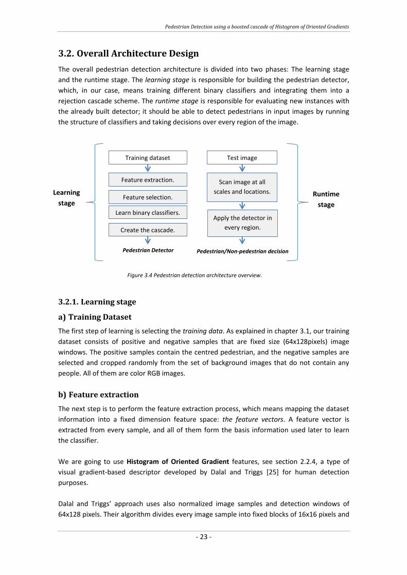
3.2. Overall Architecture Design

The overall pedestrian detection architecture is divided into two phases: The learning stage

and the runtime stage. The learning stage is responsible for building the pedestrian detector,

which, in our case, means training different binary classifiers and integrating them into a

rejection cascade scheme. The runtime stage is responsible for evaluating new instances with

the already built detector; it should be able to detect pedestrians in input images by running

the structure of classifiers and taking decisions over every region of the image.

3.2.1. Learning stage

a) Training Dataset

The first step of learning is selecting the training data. As explained in chapter 3.1, our training

dataset consists of positive and negative samples that are fixed size (64x128pixels) image

windows. The positive samples contain the centred pedestrian, and the negative samples are

selected and cropped randomly from the set of background images that do not contain any

people. All of them are color RGB images.

b) Feature extraction

The next step is to perform the feature extraction process, which means mapping the dataset

information into a fixed dimension feature space: the feature vectors. A feature vector is

extracted from every sample, and all of them form the basis information used later to learn

the classifier.

We are going to use Histogram of Oriented Gradient features, see section 2.2.4, a type of

visual gradient-based descriptor developed by Dalal and Triggs [25] for human detection

purposes.

Dalal and Triggs’ approach uses also normalized image samples and detection windows of

64x128 pixels. Their algorithm divides every image sample into fixed blocks of 16x16 pixels and

Test image

Scan image at all

scales and locations.

Apply the detector in

every region.

Pedestrian/Non-pedestrian decision

Training dataset

Feature extraction.

Feature selection.

Learn binary classifiers.

Create the cascade.

Pedestrian Detector

Learning

stage Runtime

stage

Figure 3.4 Pedestrian detection architecture overview.


- 24 -

every block contains four cells of 8x8 pixels. It creates a 9-bin Histogram of Oriented Gradients

per cell, and, concatenating the histograms of the four cells, a 36-D feature vector per block is

obtained. Features are extracted from all blocks in the entire image, with an overlap of 8 pixels

between adjacent blocks. In total, every image sample contains 7x15 blocks, which

corresponds to a 3780-D feature vector. The binary classifier is trained over this high

dimensional feature space.

Our implementation is based on the same idea, but, instead of extracting HOGs from the

entire image sample, we are going to deal only with a subset of blocks in the image. What is

more, we introduce the use of blocks at multiple scales; therefore, the selected subset can

contain blocks of different sizes ranging from 12x12 to 64x64, always with an even number of

rows and columns. Moreover, we apply an overlap of 8 pixels, to define and restrict the

possible positions of the blocks in the image sample. Consequently, the overall combinations

of positions and sizes bring a total of 1351 possible blocks.

Each of the blocks, independently of its size, is divided into 2x2 cells; and, from each of the

four cells, a 9-bin Histogram of Gradients is created. Therefore, every block is going to

transform always in a 36-D feature vector.

c) Feature selection and classification

The idea of our methodology is to collect a small subset of blocks, placed at different positions

and scales in a sample image, and extract a 36-D HOG feature vector from each block and from

each image in the training dataset. Then, train a classifier for each of the blocks and combine

the classifiers results to make the final classification/detection decision.

The selection of the subset of blocks and the way of combining the classifiers trained over each

of these blocks is implemented using the AdaBoost algorithm, as explained in section 2.3.3.c)

and in [48]. So, we are going to create a final strong classifier that consists of an ensemble of

weak classifiers, each of which tries to separate the dataset into positives and negatives using

the information of a single feature block.

We use linear Support Vector Machines, see section 2.3.1, as our baseline binary weak

classifier. They are proven to be the most accurate, reliable and scalable of all classifiers in

Dalal’s [66] experiments. They can usually converge reliably, they can manage large datasets

and they show a good robustness to different employed feature sets and learning parameters.

Moreover, the reason of using only linear classifiers, avoiding the use of kernel SVMs, is

because their run time is significantly lower.

The strong classifier should be constructed with the combination of the SVMs that best

perform. That means the ones that introduce lowest misclassification rate, subsequently, the

ones trained over the feature blocks that best discriminate the positives from the negatives. In

every round of the AdaBoost algorithm, a certain number of weak classifiers are trained and

only the one that performs the best (lowest error) is picked to be added to the strong final

classifier. Evaluating in every time all possible blocks in an image is computationally very


- 25 -

expensive, that is why we are going to evaluate only a certain reduced and fixed number (N) of

blocks (and classifiers) in each round.

The number of rounds in the AdaBoost (k) is decided according to an accuracy criterion, the

system keeps adding weak classifiers until the strong classifier reaches a desired minimum true

positive rate (dmin) and maximum false positive rate (fmax). In particular, the desired true

positive rate determines the value of the decision threshold (th) associated with the strong

classifier; meanwhile the false positive rate determines the overall number of weak classifiers.

Figure 3.5 Feature selection by AdaBoost methodology.

d) Cascade structure

Finally, we construct a rejection cascade, see section 2.3.3.d), where each level corresponds to

a strong classifier. We train levels of the cascade (i) until a system target false positive rate

(F_target) is achieved, which is calculated as the product of false positive rates (f) from every

single level in the cascade. There exists an accuracy trade off, because every new stage of the

cascade will improve the overall false positive rate (F) but also will decrease the overall true

positive rate (D).

The advantage of building cascade structure instead of a more complex and large single strong

classifier is that runtime speed can be significantly improved. The main reason is that in a

single image the majority of regions are negatives which are going to be rejected in early

levels, and only positive regions, which are exceptional events, will need to go through all

levels of the cascade.


- 26 -

Figure 3.6 Cascade of ensemble of SVMs structure.

During the learning process, it is crucial how to resample the negatives in the dataset at every

level of the cascade. One common option is to keep the negatives that have not been rejected

yet and refill the set with new ones. However, in our case, every stage of the cascade is going

to train with a completely new set of negatives samples. These negative samples are selected

randomly and evaluated through the cascade to ensure that they are still misclassified.

3.2.2. Runtime stage

The runtime or detection stage consists in a dense and multi-scale image scanning process,

where we use a sliding window that gradually is moved along different positions and grows in

scale to evaluate all regions in the image. Every region is analysed with the previously built

detector, each strong classifier of the cascade is applied sequentially, extracting first the HOGs

features and then deciding according to the level decision threshold. Once one region is

classified as a negative or when the last level is reached, the procedure finishes and the

evaluation continues with the next region in the image.

As the detector works in a simple window approach and in relative coordinates, we can apply

it in every region of the image independently of the position or scale. Besides, we are able to

choose the overlapping between regions and the rate at which the scale grows.


- 27 -

Figure 3.7 Pseudo-code of the pedestrian detector learning stage.

∑

Input: F_target: overall system desired false positive rate.

fmax: maximum acceptable false positive rate per cascade level.

dmin: minimum acceptable true positive rate per cascade level.

N: number of blocks evaluated per AdaBoost round.

1. Initialize global variables:

i =0; number of cascade levels.

D=1; overall system true positive rate.

F=1; overall system false positive rate.

2. Collect set of positive (Pos) and negative (Neg) samples.

3. While F > F_target:

a) Initialize level variables:

th=0; i-level strong classifier threshold.

f =1; i-level false positive rate.

d=0; i-level true positive rate.

;

;

Adaboost sample weights, where L_Pos and L_Neg are the

number of positive and negative samples respectively-

b) While fi > fmax;

i. Select randomly N feature blocks and extract 36-D HOGs.

ii. Train N linear SVMs using the training Pos and Neg set of

samples.

iii. Add the best SVM into the strong classifier.

iv. Update sample weights (W) in AdaBoost manner.

v. Evaluate the current strong classifier accuracy (fi and di)

over Pos and Neg set of training samples, decreasing the

threshold until dmin holds.

c) Compute overall accuracy ∏ and ∏

d) Resample the negative set of samples (Neg).

4. Output: Final detector - i-levels of the cascade

{ } .

Final training accuracy: F and D


- 28 -

Operative System: CentOS 6

Release 6.5 (Final)

Kernel Linux 6.2.32-431.20.3.el6.x86-64

GNOME 2.28.2

Hardware: Memory 7,6 GB

Prc. (x4): Intel(R) Xeon(R) CPU ES-1607 0 @3GHz

Figure 3.9 Specifications of computers used for running simulations.

Figure 3.8 Pseudo-code of the pedestrian detector runtime stage.

3.3. Overall System Development

3.3.1. Development environment

The system is implemented from scratch in MATLAB R2014a using a computer with the Linux

distribution Fedora. MATLAB is a high-level language and an interactive environment for

numerical computation, visualization and programming. It offers multiple tools and functions

to develop a large variety of applications in many different fields (signal processing,

communications, control systems, test and measurement, computational finance and biology).

MATLAB is widely- used specially in the academic and research world, because although it is

not fast and portable enough to integrate it in real applications, it is very intuitively and

versatile.

GitHub, a web-based hosting service for software development projects, has been used as the

main code repository via the Git revision control system. The updated version of the code is

available at https://github.com/crisrsan/hogsvm.

Simulations are run over several identical computers with the Figure 3.9 characteristics.

Input: I; image to evaluate.

Pedestrian detector – cascade of classifiers.

1. Read the image information.

2. Define scanning parameters:

minsize; minimum size of scanning window.

maxsize; maximum size of scanning window.

scale_factor: scanning window growing rate.

overlap_factor; scanning window overlap.

3. While s < maxsize;

a) Define a new scanning window position (row and column).

b) Evaluate the windowed image region with the pedestrian detector.

c) If pedestrian detected, draw the window boundary in the image.

4. Output: Number of detections.

Image with drawn detections.

https://github.com/crisrsan/hogsvm


- 29 -

3.3.2. Code structure

The code is organized in different MATLAB scripts and functions; each of them has a particular

task assigned which is described in this section. Moreover, Appendice A contains the detailed

data flowcharts providing a wide and graphical view of all the code structure and the function

interrelations.

>> learning.m

The learning.m is the principal script that initiates the pedestrian detector learning process. It

is the main system execution file where we set the learning parameters and create the cascade

structure.

It is responsible of calling the functions that prepare the training samples, both before starting

the learning process (prepare_samples.m) and at the beginning of every new level of the

cascade to regenerate the negatives (sample_negatives.m ), and also to establish the loop that

controls the building process of the cascade. It keeps training new levels of the cascade

through the function train_cascade_ilevel, until the overall false positive rate (F) is lower than

the established target (F_target).

The resultant trained cascade of classifiers will be saved in a text file (svm_classifier.txt),

created at the beginning of the learning. This file should contain the essential information

needed to apply the resultant detector in the runtime stage. The structure of the file will be

repetitive, for every added weak classifier we store the feature block normalized coordinates

(row, column and size), the name of the weak classifier (to be able to read it later) and the

weighted value to the strong classifier (alpha parameter). For every level we store also the

decision threshold and a marker (999999) indicating the end of the level.

5.937500e-01 4.687500e-02 6.875000e-01 classifiers/weak_svm_11.mat 2.048160e+00

F_target overall system desired false positive rate.

fmax maximum acceptable false positive rate per cascade level.

dmin minimum acceptable true positive rate per cascade level.

fv feature vector dimension, according to HOG parameters.

neg_w number of negative windows per negative image.

N number of blocks evaluated per AdaBoost round.

Figure 3.10 Learning parameters which value must be chosen before starting the learning and is going to remain fixed during all the process.

row column size svm_name svm_alpha

Feature block

(normalized coordinates)

Figure 3.11 One line example of the results file (svm_classifier.txt) structure.


- 30 -

In addition, a readable helper file (training_results.txt) is created to be able to track the

progress of the learning process. It contains the information that allows us to see if the

learning is progressing as it is supposed to do. For every cascade level we store the number of

training samples, the number of weak classifiers and their accuracy performance, the

accumulated and the current level training time, and the overall training accuracy achieved.

>> prepare_samples.m

This function is called only once at the beginning of the learning process, its role is to define

the positive and negative samples from the given dataset images.

We first create a text file (namelist.txt) containing a list of the names of all available dataset

images, separately for both the positives (path_positives) and negatives (path_negatives)

folders. For every normalized pedestrian image in the dataset we extract one positive sample

loading the necessary information in an array of structs (pos_info). The same procedure is

done for the negatives (neg_info), but defining more than one sample per negative image

according to the neg_w parameter.

The positives are going to remain the same during the whole training stage, meanwhile the

negatives are going to be modified at the beginning of every cascade level using the

sample_negatives() function.

>> sample_negatives.m

This is the function responsible for doing the regeneration of the negatives used in every level

of the cascade; although we resample a completely new set, the number of negative samples

is always the same. In our basis implementation we sample the same number of negatives

than positives.

Every new negative sample is defined generating randomly a position duplet (row, col) over a

specific background image. The new sample region is evaluated with the current pedestrian

detector, applying the already previously built levels of the cascade, and only adopted as a

negative if it is misclassified. The classification of every sample is done using the

classify_region() function.

filename complete path to the image.

width image horizontal dimension.

height image vertical dimension.

row vertical position of the negative/positive sample (centered point).

col horizontal position of the negative/positive sample (centered point).

size vertical dimension of the sample (128 pixels).

pixels pixel / bits intensity image information.

Figure 3.12 Fields of the training samples information structs (pos_info and neg_info).


- 31 -

>> train_cascade_i_level.m

The train_cascade_i_level() function trains and adds a new level to the cascade, it contains the

development of the AdaBoost algorithm to learn a new strong classifier.

First, it initializes the sample AdaBoost weights and then it starts the loop that controls the

generation of new weak classifiers.

Every selected weak classifier (select_svm()) has an error and a weighting alpha parameter

associated. The new weak classifier is added to the current strong classifier by saving the its

structure in a matfile (weak_svm_@ cascade_level@number_weak_classifier.mat ) and

appending its information (normalized feature region, name, alpha parameter) to the results

file (svm_classifier.txt). For every weak classifier we also obtain an array with the results of the

classification, where each position corresponds to one sample of the dataset, that contains 0

(negative sample) or 1 (positive sample). We accumulate the weak classification result, duly

weighted, to the previous ensemble of classifiers result (res) to evaluate the current strong

classifier accuracy. To do that, we compare each position of the classification array of results

(res) with an established decision threshold and classify every sample as negative or positive.

Finally, we compare the resultant classification with the original sample annotations and count

the number of true positives, false negatives, false positives and true negatives to compute the

false and true positive rate.

( )

( )

( )

( )

(3.1)

Where: tp (True Positives) = a positive sample classified as positive.

fn (False Negatives) = a positive sample classifies as negative.

fp (False Positives) = a negative sample classified as positive.

tn (True Negatives) = a negative sample classified as negative.

We repeat the procedure decreasing the threshold, whose initial value is the half of the sum of

all alpha parameters from all classifiers in the ensemble, until the desired minimum true

positive rate is reached (dmin). A new weak classifier is trained if, under the same threshold,

the false positive rate of the strong classifier under is still over the target one (fmax).

>> select_svm.m

This function performs the feature selection methodology, evaluating N number of weak

classifiers to choose the one that performs the best. The returned classifier will be added into

the strong ensemble of weak classifiers.

First, we generate randomly the feature block triplet (row, col, size); always ensuring that it is

contained inside the sample dimensions. Then, a 36-D HOG feature vector is extracted for the


- 32 -

same block in every dataset sample using the function feature_extraction(). All extracted

features are stored in the feature matrix (T), where every row corresponds to a sample and

every column to a dimension of the 36-D HOG. There is also defined an array of original

annotations (G), representing the class labels 0 (negatives) or 1 (positives), where every row

corresponds to a sample.

Next, we train an SVM over the obtained feature matrix information. To train and evaluate a

new SVM we take advantage, respectively, of the already implemented MATLAB pair of

functions: svmtrain2 and svmclassify3.

svmtrain requires the feature matrix (T) and the array of class annotations (G) as input

variables; and it returns a structure (SVMStruct) containing information about the

trained support vector machine classifier. Many additional options can be adjusted; we

only set the maximum number of iterations to ensure convergence (options.MaxIter)

and the soft margin parameter (boxconstraint).

svmclassify requires the trained SVM structure (SVMStruct) and also the feature matrix

(T) as input variables, and returns a classification results array (res) where every row

corresponds to a sample and contains the assigned class label.

According to the classification results, we compute the weak classifier error in an AdaBoost

way.

The previous procedure is repeated with N different feature blocks, and, at the end, we return

the normalized feature block coordinates, the SVM structure and the weighting alpha

parameter of the one that presented the lowest error.

>> feature_extraction.m

This function is responsible for doing the feature extraction process itself, which means

subtracting the Histogram of Oriented Gradient feature vector from a given image region in all

training samples.

To compute the HOG features we use the extractHOGFeatures4 MATLAB function. It returns a

HOG feature vector from a truecolor or greayscale input image. The additional function

options allow setting all HOG computation parameters, such as the cell or blocking size, the

block overlap, and the number of bins per histogram.

The dimension of the returned feature vector is the product of three variables: the number of

blocks per image, the blocks size and the number of bins per cell. In our case, we want a 36-D

feature vector; so, as the default number of bins per histogram is 9, we force to treat the input

2 http://www.mathworks.se/help/stats/svmtrain.html

3 http://www.mathworks.se/help/stats/svmclassify.html

4 http://www.mathworks.se/help/vision/ref/extracthogfeatures.html


- 33 -

region as a single block of 4 cells. For that purpose, we adjust the CellSize (number of pixels per

cell) parameter according to the input region (feature block) size.

hog = extractHOGFeatures(I, 'CellSize', [floor(length(I)/2) floor(length(I)/2)])

Therefore, the returned feature vector will be always 36-dimensional, independently of the

input region/ feature block size.

One feature vector is extracted over every single positive and negative sample. One by one, we

crop the region of the image (feature block) that is going to be evaluated, this step converts

the RGB image into grayscale, and we apply the extractHOGfeatures function. The resultant

36-D HOG feature vectors are stored in the feature matrix (T) which is needed afterwards for

the SVM training and evaluation.

>> classify_region.m

The classify_region() function is used both in the learning (sample of negatives) and the

runtime stage; it evaluates a given region in an image with the pedestrian detector and

classifies it as containing a pedestrian (positive) or not (negative).

The function opens the detector results file (svm_classifier.txt), and reading it sequentially is

able to apply the built cascade of classifiers to the given image region. The first step is to adjust

the normalized coordinates of the feature block to the new region size and then assess every

level of the cascade in an analogues way as done in the training stage. We extract the HOG

features (extractHOGFeatures), evaluate the correspondent linear SVM (svmclassify) and take

the classification decision according to the established decision threshold.

The function will return a 0 if the region is classified as negative, it has been rejected after

evaluating one of the intermediate levels of the cascade, or a 1 if a pedestrian is detected, the

region goes successfully through all the levels of the cascade.

>> runtime.m

This is the main file of the runtime stage; it evaluates a new image to detect the contained

pedestrians. The function requires path to the location of the image as input and returns the

number of detected pedestrian regions and the image with the detection boundaries

visualization.

The evaluation is done at different scales and positions in the image using a sliding window

that crops and classifies, calling the classify_region() function, a single region at a time. It is

possible to determine the scanning parameters: minimum (minsize) and maximum size

(maxsize) of the scanning window, the number of overlapping pixels between adjacent

evaluated regions (overlap_factor) and the size growing rate (scale_factor).


- 34 -

4. Results

4.1. Baseline detector

4.1.1. Parameters configuration

The aim in this chapter is to define a baseline training configuration to learn and test the

pedestrian detector. The resultant baseline detector performance is going to be used as a

reference for later comparisons. The training parameters that must be adapted to our

preferences are:

Overall detector accuracy - F_target: minimum false positive rate acceptable of the

whole cascade. It represents the overall detector desired accuracy and determines the

overall cascade training time and dimension as it regulates when the learning process

finishes.

Cascade level accuracy - fmax & dmin: maximum false positive rate and minimum true

positive rate, respectively, acceptable per cascade level. It regulates the number of

classifiers per cascade level as every strong classifier has to present always a minimum

accuracy.

Number of training samples - neg_w: assuming that we use all the available positive

samples, we can determine the dimension of the dataset by varying the number of

negative samples. Therefore, the neg_w parameter defines the number of windows

extracted per negative image. However, there is implemented an alternative approach

where we can just define the total number of desired negatives and they are extracted

sequentially from every background image. What is more, it is also possible to select

only a subset of the available positive samples.

Feature vector dimension – fv: the dimension of the feature vector is related to the

intrinsic Histogram of Oriented Gradients parameters, such as the number of cells per

block and the number of bins per histogram. It is possible to select first the feature

vector dimension and then adjust the HOG parameters or vice versa; the second

option is more advisable and natural.

Feature selection - N: this parameter defines the dimension of the feature selection

subset; that means, how many different feature blocks, or how many linear SVM are

trained, are tested before adding a new weak classifier to the cascade.

First, we set the previous parameters identically as they do in the reference paper [51] and,

then, we introduce slight variations in order to adapt the learning process to our conditions

(computation time, structure of the cascade, accuracy achieved…). After some trials, the final

baseline configuration values are shown in Figure 4.1.

The path to the dataset training images location, both the negatives and the positives, must be

indicated, as well as the way of regenerating the negatives in each new level of the cascade. In

that case we resample a completely new set of negatives, evaluating first that they are

misclassified by the current detector.


- 35 -

4.1.2. Learning results

After setting all the parameters, we initiate the training process by executing the learning.m

script. The classifier results (svm_classifier.txt) and tracking (training_results.txt) files are

created immediately and filled along the learning progression. Besides, the SVM structures are

also saved sequentially in the same folder. The following figures show an example of the

information contained in the resulting files after two levels of the cascade are trained:

//training_results.txt// CASCADE LEVEL1 4832samples:2416positives &2416 negatives. WEAK CLASSIFIER NUMBER1 CPUTIME128.92 Region:0.507810.265620.751 Error:0.13597 Alpha:1.8492 Threshold:0 TPR:1 FPR:1 WEAK CLASSIFIER NUMBER2 CPUTIME108.35 Region:0.132810.265620.718751 Error:0.13732 Alpha:1.8378 Threshold:0 TPR:1 FPR:1 WEAK CLASSIFIER NUMBER3 CPUTIME113.95 Region:0.00781250.265620.6251 Error:0.24961 Alpha:1.1007 Threshold:0 TPR:1 FPR:1 WEAK CLASSIFIER NUMBER4 CPUTIME137.59 Region:0.00781250.140620.68751 Error:0.34838 Alpha:0.62617 Threshold:0.6169 TPR:0.99752 FPR:0.37417 Final stage threshold:0.6169 Computation time STAGE:503.85 Computation time TOTAL:578.69 Final stage F:0.37417 Final stage D:0.99752 CASCADE LEVEL2 4832samples:2416positives &2416 negatives.

WEAK CLASSIFIER NUMBER1 CPUTIME142.84 Region:0.757810.390620.51 Error:0.1666 Alpha:1.6099 Threshold:0 TPR:1 FPR:1 WEAK CLASSIFIER NUMBER2 CPUTIME158.24 Region:0.0703120.390620.6251 Error:0.22703 Alpha:1.2252 Threshold:0 TPR:1 FPR:1 WEAK CLASSIFIER NUMBER3 CPUTIME156.29 Region:0.382810.0156250.656251 Error:0.21584 Alpha:1.2901 Threshold:0 TPR:1 FPR:1 WEAK CLASSIFIER NUMBER4 CPUTIME147.66 Region:0.195310.140620.593751 Error:0.24788 Alpha:1.11 Threshold:0 TPR:1 FPR:1 WEAK CLASSIFIER NUMBER5 CPUTIME146.9 Region:0.445310.265620.281251 Error:0.34814 Alpha:0.62723 Threshold:0.62121 TPR:0.99752 FPR:0.59561 Final stage threshold:0.62121 Computation time STAGE:770.31 Computation time TOTAL:1646.28 Final stage F:0.22286 Final stage D:0.99504

Overall accuracy: F_target 1·10-6

Level accuracy: fmax 0.65

dmin 0.995

Dataset: neg_w number of negatives = number of positives = 2416

Feature vector: fv 36

Feature selection: N 5

Figure 4.1 Baseline parameter values

Figure 4.2 Two-level cascade resultant training_results.txt content example


- 36 -

Figure 4.3 Two-level cascade resultant svm_classifier.txt content example.

Due to lack of resources, which mainly means computation power and time, we decide to

learn only the first 10 levels of the cascade.

After 101 hours of computer execution, the resultant cascade consists of 10 levels and 373

weak classifiers (linear SVMs). The number of classifiers per level, and consequently the

strong classifiers complexity, increases exponentially through the cascade.

Figure 4.4 (a) In grey color, the number of weak SVM classifiers in each level of the cascade. (b) In blue color, the rejection rate as cumulative sum over cascade levels.

However, the number of rejected negatives decreases considerably along the cascade, the

accumulated rejection rate results in an inverse exponential function. The first three levels in

our cascade only contain less than ten classifiers each and reject about 80% of the detection

windows. The earlier stages contain simpler strong classifiers responsible of roughly reject

most of the negatives and as we progress through the cascade the levels become more

complex. These later classifiers are responsible of tuning in detail the detector performance

trying to properly classify the more challenging negatives.

According to the training results, the ten first levels bring an overall true positive rate of

95,658% and a false positive rate of 0,598%.

0

0,1

0,2

0,3

0,4

0,5

0,6

0,7

0,8

0,9

1

0

20

40

60

80

100

120

140

160

1 2 3 4 5 6 7 8 9 10

Nº

clas

sifi

ers

Cascade level

// svm_classifer.txt // 5.078125e-01 2.656250e-01 7.500000e-01 1 classifiers/weak_svm_11.mat 1.849186e+00 1.328125e-01 2.656250e-01 7.187500e-01 1 classifiers/weak_svm_12.mat 1.837760e+00 7.812500e-03 2.656250e-01 6.250000e-01 1 classifiers/weak_svm_13.mat 1.100696e+00 7.812500e-03 1.406250e-01 6.875000e-01 1 classifiers/weak_svm_14.mat 6.261671e-01 999999 6.169045e-01 7.578125e-01 3.906250e-01 5.000000e-01 1 classifiers/weak_svm_21.mat 1.609935e+00 7.031250e-02 3.906250e-01 6.250000e-01 1 classifiers/weak_svm_22.mat 1.225169e+00 3.828125e-01 1.562500e-02 6.562500e-01 1 classifiers/weak_svm_23.mat 1.290105e+00 1.953125e-01 1.406250e-01 5.937500e-01 1 classifiers/weak_svm_24.mat 1.109975e+00 4.453125e-01 2.656250e-01 2.812500e-01 1 classifiers/weak_svm_25.mat 6.272343e-01 999999 6.212087e-01


- 37 -

4.1.3. Runtime results

Once the detector structure is created we can test its operation and analyse its behaviour. To

study the performance of the resultant trained detector we categorize the testing dataset, see

3.1, and compute the accuracy rates (true positive and false positive rates) over the achieved

classification results.

We classify every positive image in the testing dataset (1132 positive samples in total), using

the classify_region() function, and obtain the number of detections (true positives). We repeat

the same procedure with the negative samples, defining three negative windows per testing

image (1359 negative samples in total), and obtain again the number of detections (false

positives). Finally, as we also know how many positive (the total of positives correspond to the

sum of true positives and false negatives) and negative (the total of negatives correspond to

the sum of false positives and true negatives) samples have been evaluated in total, we

calculate the correspondent accuracy rates.

The baseline detector presents a 95,94% True Positive Rate and 1,398% False Positive Rate.

Varying the decision threshold it is possible to compute different accuracy rates and draw the

Receiver Operating Characteristic (ROC) curve, Figure 4.5. This curve illustrates the overall

performance of our binary classification system.

Figure 4.5 Baseline detector ROC curve.


- 38 -

The classification time is 0,227 seconds, on average, for a negative window and 8,813 seconds

for a positive window.

Additionally, some complete scanning evaluations, using the runtime() function, over full

positive and negative images are also executed. The following figures show graphically the

accumulated regression results, which mean the pedestrian detector numeric result before

applying the classification decision threshold, for every evaluated image window. In positive

images, the pedestrian region is detected properly at many different positions and scales. In

the example background image, Figure 4.7, most of the false positives appear concentrated

around two hot spots, which must correspond to regions with a feature structure quite similar

to the pedestrian one.

Plotting the regression results evidences that some post-processing techniques can be very

useful to improve the detector final performance giving practicality to make it able to work in

real situations (detailed explanation in conclusion chapter 5).

Figure 4.6 Scanning window accumulated classification results over a positive sample.


- 39 -

Figure 4.7 Scanning window accumulated classification results over a negative sample


- 40 -

4.2. Sensitivity analysis

The objective of this section is to analyse how the different training parameters influence in

the resultant pedestrian detector in terms of the learning process development, the cascade

structure obtained and the runtime performance.

This comparison is going to do through a sensitivity analysis which consists in varying only one

parameter at a time and observe the changes in the learning and runtime processes behaviour

and results. The study will take into account the most significant learning parameters: feature

blocks geometry, feature (HOG) and classifier (SVM) parameters, dataset dimension, feature

selection technique, the way of resampling the negatives and the type of classifier employed.

4.2.1. Feature blocks geometry

The first study carried out involves the type of blocks over which we compute the HOG feature

vector. The baseline implementation uses only square blocks of different sizes with an overlap

of 8 pixels; the feature set contains 1351 different possible blocks. We modify the available set

of feature blocks trying two different approaches.

The first one reduces the set dimension defining only square blocks of a fix size of 16x16

pixels, going backwards to the original Dalal and Triggs proposal [25]. With an overlap of 8

pixels, the total number of possible blocks is 91.

The second approach expands the feature block set, as in [51], introducing not only different

block sizes but also different aspect ratios. The possible aspect ratios are (1:1), (1:2), (2:1);

therefore, the feature set contains both square and rectangular blocks variable in size, from

12 to 64 pixels width. The overlap varies depending on the block size, obtaining a feature set of

4353 possible blocks.

On the one hand, the approach with fix blocks doesn’t achieve convergence after more than

200 hours of training; we are able to finalize the learning of only 7 levels of the cascade that

contain 144 classifiers and give a 97,08% TPR and 8,756 % FPR. This accuracy performance

cannot be compare fairly with the baseline, because as it refers to less levels of the cascade

(only 7 out of 10) it is logical that it presents a better TPR and a worse FPR, as a consequence

of the mentioned trade-off between both ratios as we keep adding levels to the cascade.

Baseline Fix blocks Rectangular blocks Learning stage results

Training time 101 h ~10h 42 h Levels of the Cascade 10 7 10 Number of Classifiers 373 144 274

Accuracy performance TPR 95,94% 97,08% 95,85% FPR 1,398% 8,756% 1,398%

Testing time (seg) Positive window 8,8 1,6149 2,8713 Negative window 0,227 0,4918 0,1916

Table 4.1 Feature blocks geometry comparative analysis


- 41 -

On the other hand, the approach with rectangular blocks lasted 42h to train 10 levels of the

cascade, and the resultant system has 274 classifiers and gives 95,85% TPR and 1,398% FPR.

The accuracy performance is nearly the same than the offered by the baseline configuration,

but the training time is reduced to more than a half. Furthermore, the number of classifiers is

lower which is translated in higher runtime speed.

As a general conclusion, we observe that it is better to have a larger feature set. The more

available different feature blocks, the more possibilities to find a suitable combination of

features to describe the target object. In the case of fix-sized blocks, the possible combinations

are not enough informative to create a functional classification system. As we enlarge and

diversify the feature set, the system finds suitable combinations more easily; less training time

is required to achieve the same accuracy. In particular, introducing rectangular blocks enhance

the performance because they can represent better the pedestrian structure (legs, body,

arms…). The human body proportions are similar to the rectangular blocks we use as the width

of a pedestrian figure is generally 40-50% of the height.

Figure 4.8 Zoomed detail of the ROC curves of the different blocks geometry.

If we plot the ROC curves of the three tested solutions, we can clearly see that the one

including rectangular blocks out-perform slightly the baseline approach. The information given

by the approach with fix blocks is not reliable enough to draw a proper line.

4.2.2. Histogram of Oriented Gradients computation

Interesting comparisons result from varying the intrinsic parameters of the extracted features

(HOG) and the employed classifier (SVM). Both operations have been computed using given

MATLAB functions which offer many different additional options that can be adjusted

straightforwardly.


- 42 -

In the case of the feature extraction, we can decide how the Histograms of Oriented Gradients

are computed in terms of number of pixels per cell, number of cells per block, block overlap

and number of bins per histogram.

As every evaluated image region should correspond always to only one block, we modify,

separately, the number of bins per histogram and the number of cells per block.

The baseline configuration uses 9 bins per histogram and 2x2 cells per block; the simulations

executed try 4 and 18 bins per histogram, and 1x1, 4x4 and 8x8 cells per block.

It is relevant to have in mind that every time we change one of the previous parameters, the

dimension of the final extracted feature vector (fv) is altered too. So, the obtained variations

will rely mainly in how large is the feature vector, or, what is the same, the amount of

information that the extracted features contain.

Number of bins Block Size Baseline 18 4x4 8x8 36-D 72-D 144-D 576-D

Learning stage results Training time 101 h 35 h 53 h 78 h

Levels of the Cascade 10 10 10 10 Number of Classifiers 373 183 162 55

Accuracy performance TPR 95,94% 96,67% 95,67% 91,34% FPR 1,398% 1,251% 1,545% 1,398%

Testing time (seg) Positive window 8,8 3,284 4,630 3,920 Negative window 0,227 0,260 0,230 10,14

Table 4.2 HOG extraction parameters comparative analysis.

When we reduce the feature vector dimension under 36-D, 4 bins per histogram and 1x1 cells

per block, the execution gets stuck in the very early levels and doesn’t get to any convergence.

On the contrary, as we increase the feature vector dimension over 36-D, modifying either the

number of bins or the number of cells per block, the time required to train 10 levels of the

cascade is reduced significantly. This is the case when using 18 bins or 4x4 cells per block; not

only the learning time decreases but also the overall number of classifiers and the testing time

are reduced while an accuracy performance similar to baseline configuration is maintained,

see Table 4.2.

Nevertheless, there exists a limit when the feature vector dimension becomes too large that it

slows the training process and also leads to overfitting situations. Overfitting means training

an algorithm with too much specific information relative to the training data, which results in a

system trained and adapted specifically to the training data and with generally a poor

classification performance over new examples.


- 43 -

In our experiment, the overfitting phenomenon occurs in the case of 8x8 cells per block, where

the training time is reduced slightly but the accuracy performance worsens considerably. In

addition, the number of classifiers is reduced to less than a sixth part of the classifiers in the

baseline approach and the theoretic baseline overall false positive rate is achieved only with

four levels of the cascade, these facts show how the system is able to completely adapt its

structure to the training dataset.

Figure 4.9 Zoomed detail of the ROC curves of the different block sizes.

4.2.3. SVM soft margin

Adopting linear SVM classifiers restrict the variation possibilities over intrinsic classification

parameters. We decide to evaluate different grades of misclassification tolerance by changing

the classifier soft margin parameter (c). This parameter, called Box Constraint in the MATLAB

terminology, controls the maximum penalty imposed on margin-violating observations and

helps to prevent overfitting. As the Box Constraint increases, the classifier becomes less

permissive in terms of the accepted number of misclassified samples when establishing the

classification function.

With extreme values of c, smaller (c=2·10-3) or higher (c=10), the system doesn’t achieve

convergence. However, with reasonable variations, see Table 4.3, the behaviour of the

learning and the testing stages remains almost unalterable.

This little performance difference can be seen in the ROC curves graphic where all curves

follow the same tendency and they are plotted much closed to each other, among all a Box

Constraint of 0.2 seems to perform the best.


- 44 -

Baseline c = 0,5

c = 0,2 c = 1

Learning stage results Training time 101 h 60 h 71 h

Levels of the Cascade 10 10 10 Number of Classifiers 373 324 368


Testing time (seg) Positive window 8,8 5,6089 9,4688 Negative window 0,227 0,2861 0,7288

Table 4.3 SVM soft margin constraint parameter comparative analysis.

Figure 4.10 Zoomed detail of the ROC curves of the different SVM soft margin constraints.

If we allowed the use of non-linear kernel functions, there will appear new possible

combinations of parameters to investigate. But we keep using only linear SVMs because the

reference implementation relies on the idea to take advantage of their simplicity and

computational speed.

4.2.4. Number of training samples

As commented previously in the section 3.1, the composition of the dataset is fundamental for

the learning process development. Once decided which dataset to be used, it is also important


- 45 -

to define properly its dimension. As the number of positive samples is often limited, the

decision usually implicates varying the number of negative samples.

It is recommendable to use at least the double number of negatives than positives. The

baseline configuration uses the same number of negatives than positives, which is 2416

samples per class and corresponds to, approximately, two negative windows per background

image. In the sensitivity analysis simulation we define ten negative windows (neg_w) per

background image, according to the INRIA Dataset providers’ original recommendation, which

results in a total number of 12180 negative samples.

Baseline 2416 negatives

12180 negatives

Learning stage results Training time 101 h 550 h

Levels of the Cascade 10 10 Number of Classifiers 373 404

Accuracy performance TPR 95,94% 96,55% FPR 1,398% 1,104%

Testing time (seg) Positive window 8,8 10,93 Negative window 0,227 0,618

Table 4.4 Dataset dimension comparative analysis.

The training time is five times higher and the number of classifiers is also slightly larger.

However, although the difference is very small (0,610% in TPR and 0,294% in FPR), the

accuracy performance is better in both terms of true positive and false positive detections.

4.2.5. Feature selection subset dimension

Related with the AdaBoost algorithm implementation, we are going to analyse how influences

the dimension of the feature selection subset. Increasing the number of weak classifiers

trained in every boosting round, we increase the probability of finding a more suitable

classifier.

The baseline configuration starts sampling only 5 blocks. The ideal situation would be trying all

the possible feature blocks in every round, but this is excessive time consuming. However, we

try a sufficiently high number instead that ensures the same performance according to the

Scholkopf & Smola sampling methodology [67]. Their theorem exemplifies that in order to

obtain an estimate that is with probability 0.95 among the best 0.05 of all estimates, a random

sub-sample of size log0.05/log0.95 = 59 will guarantee nearly as good performance as if we

considered all the random variables. In practice we sample 210 feature blocks, which satisfies

the mentioned condition for both the baseline and the rectangular blocks configurations.

The performance results are better than the baseline in terms of false positives detection but

worse in number of true positives. However, all in all, we conclude that is better to enlarge the


- 46 -

feature selection set because although the training time is doubled, the number of classifiers is

reduced further improving the testing time.

Baseline N=5

N = 210

Learning stage results Training time 101 h 226 h

Levels of the Cascade 10 10 Number of Classifiers 373 175



Table 4.5 Feature selection subset dimension comparative analysis.

4.2.6. Negatives resampling technique

There exist many different ways of treating the resampling of negatives at the beginning of

every new level of the cascade. In the baseline configuration the set of negatives is fully

randomly resampled. In the sensitive analysis we learn the detector without resampling the

negative set, which means keeping only the negatives that have been misclassified and not

regenerating new ones. Consequently, the number of negatives decreases in every new level

of the cascade and the learning process finishes because the system runs out of negative

samples.

The results differ significantly from the ones obtained with the baseline configuration,

confirming the importance of the negatives resampling treatment. The training stage lasted

only 1,1 h and the cascade contains 50 classifiers and brings an accuracy of 95,67% TPR and

5,077% FPR. It is just a coincidence that the cascade consists of 10 levels; although we would

dispose of the required time or computation power, we would never be able to train more

levels of the cascade without regenerating the negatives.

Baseline No resampling Learning stage results

Training time 101 h 1,1 h Levels of the Cascade 10 10 Number of Classifiers 373 50



Table 4.6 Negatives resampling methodology comparative analysis.


- 47 -

Another approach, consisting in keeping always the same set of negatives and only replenish

the ones that have been already correctly detected, was also implemented. In that case, but,

the training couldn’t have done because the system got stuck in the very early stages.

The experiment has been useful to confirm that most of the consumed learning time is

employed to regenerate the negatives and that the negatives availability restricts the

attainable accuracy.

4.2.7. Typology of weak classifier

Finally, the last analysis carried out consisted on changing the typology of employed classifier.

Instead of SVMs we use decision trees as the basis weak classifiers. The implementation is

done using the MATLAB functions fitctree5, for the training, and predict6, for the evaluation.

The aforementioned functions operate analogously to the SVM functions, so only very small

modifications need to be introduced in the code.

The other parameters are configured as the baseline detector and the obtained results are

surprisingly dissimilar. The training time is reduced to only 4h and the trained cascade contains

6 levels with 2 classifiers per level. The performed accuracy is really poor in terms of detection

rate, 62,630 % true positive rate. However, the performance over the training dataset is

0,876% FPR and 99,100% TPR, which shows that we are clearly facing a situation of overfitting.

Trying to solve the problem, the same structure was trained incrementing the dataset

dimension to 12180 negative samples. The obtained results are even worse according to the

tested accuracy.

Decision Tree Baseline Baseline 12180 negatives

Learning stage results Training time 101 h 4 h 96 h

Levels of the Cascade 10 6 4 Number of Classifiers 373 12 11


Testing time (seg) Positive window 8,8 0,058 - Negative window 0,227 0,170 -

Figure 4.11 Typology of classifier (decision tree) comparative analysis.

The repeatedly overfitting, which doesn’t depend on the number of training samples, evidence

that further modifications need to be done in order to adapt the system for working with

decision trees.

5 Feature selection subset dimension comparative analysis.

6 Feature selection subset dimension comparative analysis.


- 48 -

5. Conclusions

5.1. Technical conclusions

Along the chapter 4.Results, particular conclusions of every evaluated configuration have been

already exposed. However, this section summarizes the main general conclusions that we can

extract from the overall implemented work.

The sensitivity analysis illustrates that, in our implementation, modifying the training variables

do not change meaningfully the final accuracy performance of the detector. The maximum

experimented variation is 2,030% in the TPR and 0,836% in the FPR. Nevertheless, changes in

the training variables configuration affect considerably the learning process development,

mainly in terms of training time and complexity of the resultant cascade of classifiers. This is a

logical behaviour according to how the learning stage is defined; in order to build the cascade,

desired target accuracies are set, both for the overall cascade and the individual levels, as the

training terminating conditions. The behaviour would be different if the terminating criterion

refers to other aspects than accuracy; for example, we could have fixed the maximum number

of classifiers per level or the maximum number of levels in the cascade.

The sensitivity analysis allowed also observing and understanding the overfitting and

underfitting, or not convergence, problems. Both are extreme undesired situations that lead to

poor prediction on new samples, therefore, the training parameters should be chosen to avoid

both phenomena. However, there exists always a trade-off between them. On the one hand,

overfitting occurs when the system has too much detailed information of the training dataset

and is able to learn a perfect model that even describes the noise of the data; on the other

hand, underfitting or unconvergence situations occur because the system has not enough

information to find a suitable model to represent the trend of the data. It is a must to know

the behaviour of our system and define the value boundaries, or value range, to properly set

every training parameter. For example, in our implementation, the SVM soft margin constant

value must be between 0.1 and 1 to achieve convergence; besides, the HOG feature vector

dimension should be lower than 576 to avoid over training the system.

Among all the different evaluated cases, it is imperative to highlight the importance of the

negatives resampling strategy. The way of resampling the negatives influences directly and

significantly not only to the achieved detector accuracy but also to the computation speed of

the training process. It is crucial to define a proper way of treating the negative samples, being

creative to discover new useful and specifically adapted approaches but also consistent with

the learning process definition. Our solution introduces randomness for a complete renovation

of the negative set at the beginning of every level, which ensures convergence and consistency

at the expense of a large computational cost. The resampling of the negatives is the most

computationally expensive task of the whole learning process, the time it takes to resample a

new set of negatives increases exponentially as we progress along the cascade because it

becomes more difficult to find new false positive regions.


- 49 -

Last but not least, according to the sensitivity analysis results, it is possible to determine that

the final accuracy performance of a pedestrian detector relies mainly on the type of feature

extracted. This statement, which confirms the importance of feature selection and extraction

processes, is evidenced because the largest performance variations happened when modifying

the intrinsic parameters of the HOG extraction (number of bins per histogram, number of cells

per block…). The extracted feature vector represents the basic information among which the

classification model is built and the decisions are taken; therefore, it should be as accurate,

representative and discriminative as possible.

5.2. Future work

Focusing in the present work, there are several possible lines of imminent future work to bring

improvements.

First, extending the training and testing datasets, both in terms of dimension and complexity,

could be an interesting practice to adapt the detector implementation accordingly to the

observed behaviour. It would be worth to learn and test the detector with bigger datasets

incrementing the number of positive and negative samples. The INRIA Person Dataset contains

a limited number of positive samples, so it is only possible to enlarge the negative set.

However, it would be also interesting to test other pedestrian datasets which will vary in

dimension and also in complexity of the contained objects. There are simpler datasets

available, with plain backgrounds and a more limited set of poses, and also more challenging

datasets, with a larger range of poses or presenting object occlusions.

In a first debugging stage, we have used the MATLAB profile function through the Profiler

graphical user interface. This function tracks the execution time of the code files and it was

very useful to detect the critical points and change the code structure to reduce computation

time. However, a lot of work in code optimization can still be done to enhance efficiency,

always having in mind MATLAB speed limitations. A further solution will be translating the

implementation to a faster and real applying programming language (combination of C and

OpenCV).

Moreover, introducing little modifications to the core classification elements, features and

classifiers, can lead to big improvements. Regarding the feature extraction process, it would be

valuable to use color information when computing the HOGs; the current implementation

works over greyscale images because they are converted when cropping the image region with

MATLAB. Besides, it would be interesting trying to implement different HOG computations,

such us introducing integral image or integral histogram concepts, which will enhance

efficiency, or exploring a way to adapt the feature vector dimension to the region size. About

the employed weak classifiers, a first approach would be to introduce variations in the SVM

definition using the MATLAB function options, specially trying the use of non-linear kernels.

In addition, we could develop the idea of trying different typologies of basic classifiers and,

specially, adapting the system to decision trees. In the first trials, we have seen that the

current implementation with decision trees leads to over fitting situations, but it showed first


- 50 -

signs of low computation time and less complexity of the cascade. A possible solution would

be using random forests.

Finally, we can always add additional improvements that have nothing to do with the intrinsic

classification algorithm but that can prepare the detector to be used in real applications.

Referring mainly to pre and post-processing techniques such as, background modelling or

clustering detections. Beneficial possibilities rely on using time and spatial information as key

factors, to, for example, accumulate evidence over different frames in video sequences, where

the false alarms are typically blinking and true detections appear in clusters, in both spatial and

time domain. Ultimately, it is to take advantage of the real world information to think in a

practical way and being able to adapt and apply the current detector to real situations.


- 51 -

Appendices

A. Data flowcharts

Figure A.1 Overall code structure.

k ++;

path_positives & path_negatives

YES

?

F > F_target

NO

i ++;

learning. m

prepare_samples ()

train_cascade_ilevel ()

pos_info & neg_info

END TRAINING

sample_negatives ( )

?

FPRi > fmax

select_svm ()

YES

?

TPRi < dmin

YES

Decrease threshold

NO

NO

classify_region ( )

feature_extraction ( )


- 52 -

Figure A.2 File learning.m structure and operation.


- 53 -

Figure A.3 File train_cascade_i_level.m structure and operation.


- 54 -

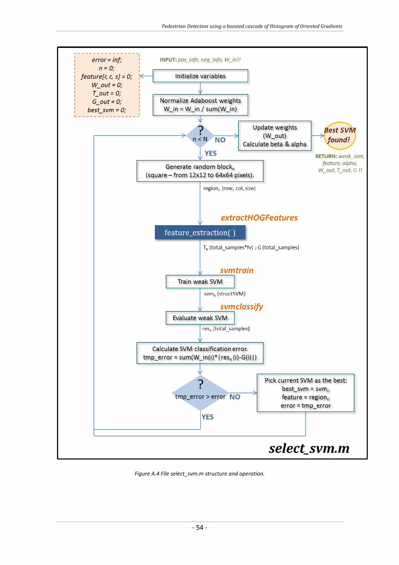
Figure A.4 File select_svm.m structure and operation.


- 55 -

List of Figures

Figure 2.1 Object detection general structure. ............................................................................................. 3

Figure 2.2 A set of extended Haar like features [18]; a) edge features, b) horizontal and vertical line

features, c) diagonal line features and d) center-surround features and special diagonal features. ........... 5

Figure 2.3 Original pedestrian image, horizontal and vertical gradient images. ............ 8

Figure 2.4 Gradient magnitude (m) and orientation (θ). .............................................................................. 8

Figure 2.5 Original image and the correspondent Histograms of Oriented Gradients. ................................ 9

Figure 2.6 Computation of Histograms of Oriented Gradients ..................................................................... 9

Figure 2.7 Classification as the task of mapping an input instance x, with an attribute set v, into its class

label y. ........................................................................................................................................................ 10

Figure 2.8 Two-dimension linear SVM representation; choosing the hyperplane that maximizes the

margin (h1). ................................................................................................................................................ 11

Figure 2.9 Binary decision tree with binary classification (classes y1 and y2). Where x is the sample to be

classified, v is the feature vector associated to the sample, fn are the attribute test conditions (split

functions) and tn the thresholds in each n node conditions. ....................................................................... 12

Figure 2.10 Pseudo-code of the bagging ensemble algorithm. .................................................................. 14

Figure 2.11 Bagging ensemble binary classifier (classes y1 and y2) of K decision binary trees. Where Sk

are the different subsets of training samples,x is the sample to be classified, v is the feature vector

associated to the sample, fn,k are the attribute test conditions (split functions) and tn the thresholds in

each n node and k tree. .............................................................................................................................. 14

Figure 2.12 Pseudo-code of the random forest algorithm .......................................................................... 15

Figure 2.13 Pseudo-code of the adaptive boosting algorithm – Adaboost. ............................................... 17

Figure 2.14 Cascade of binary classifiers structure..................................................................................... 18

Figure 3.1 Examples of negatives and positives images from the INRIA Person Dataset. .......................... 22

Figure 3.2 Generation of positive samples. ................................................................................................ 22

Figure 3.3 Generation of negative samples. ............................................................................................... 22

Figure 3.4 Pedestrian detection architecture overview. ............................................................................. 23

Figure 3.5 Feature selection by AdaBoost methodology. ........................................................................... 25

Figure 3.6 Cascade of ensemble of SVMs structure. ................................................................................... 26

Figure 3.7 Pseudo-code of the pedestrian detector learning stage. ........................................................... 27

Figure 3.8 Pseudo-code of the pedestrian detector runtime stage. ........................................................... 28

Figure 3.9 Specifications of computers used for running simulations. ....................................................... 28

Figure 3.10 Learning parameters which value must be chosen before starting the learning and is going to

remain fixed during all the process. ........................................................................................................... 29

Figure 3.11 One line example of the results file (svm_classifier.txt) structure. .......................................... 29

Figure 3.12 Fields of the training samples information structs (pos_info and neg_info). .......................... 30

Figure 4.1 Baseline parameter values ........................................................................................................ 35

Figure 4.2 Two-level cascade resultant training_results.txt content example ........................................... 35

Figure 4.3 Two-level cascade resultant svm_classifier.txt content example. ............................................. 36

Figure 4.4 (a) In grey color, the number of weak SVM classifiers in each level of the cascade. (b) In blue

color, the rejection rate as cumulative sum over cascade levels. ............................................................... 36

Figure 4.5 Baseline detector ROC curve. ..................................................................................................... 37

Figure 4.6 Scanning window accumulated classification results over a positive sample. .......................... 38

Figure 4.7 Scanning window accumulated classification results over a negative sample .......................... 39

Figure 4.8 Zoomed detail of the ROC curves of the different blocks geometry. ......................................... 41

Figure 4.9 Zoomed detail of the ROC curves of the different block sizes. ................................................... 43

Figure 4.10 Zoomed detail of the ROC curves of the different SVM soft margin constraints. ................... 44

Figure 4.11 Typology of classifier (decision tree) comparative analysis. .................................................... 47


- 56 -

Figure A.1 Overall code structure. .............................................................................................................. 51

Figure A.2 File learning.m structure and operation. ................................................................................... 52

Figure A.3 File train_cascade_i_level.m structure and operation. ............................................................. 53

Figure A.4 File select_svm.m structure and operation. .............................................................................. 54


- 57 -

List of Tables

Table 4.1 Feature blocks geometry comparative analysis .......................................................................... 40

Table 4.2 HOG extraction parameters comparative analysis. .................................................................... 42

Table 4.3 SVM soft margin constraint parameter comparative analysis. .................................................. 44

Table 4.4 Dataset dimension comparative analysis. .................................................................................. 45

Table 4.5 Feature selection subset dimension comparative analysis. ........................................................ 46

Table 4.6 Negatives resampling methodology comparative analysis. ....................................................... 46


- 58 -

References

[1] R. Szeliski, "Object detection," in Computer Vision: Algorithms and Applications, Springer,

2010, pp. 658-666.

[2] L. Fei-Fei, R. Fergus and A. Torralba, "Recognizing and learning object categories,"

[Online]. Available: http://people.csail.mit.edu/torralba/shortCourseRLOC/.

[3] M. Nixon and A. Aguado, Feature Extraction and Image Processing, Elsevier Ltd., 2008.

[4] I. Guyon and A. Elisseeff, "An Introduction to Feature Extraction," in Feature Extraction,

Foundations and Applications, Springer, 2006, pp. 1-25.

[5] D. p. Tian, «A review on image feature extraction and representation techniques,»

International Journal of Multimedia and Ubiquitous Engineering, vol. 8, nº 4, pp. 385-396,

July 2013.

[6] D. A. Lisin, M. A. Mattar, M. B. Blaschko, M. C. Benfield and E. G. Learned-Miller,

"Combining Local and Global Image Features for Object Class Recognition," Proceedings of

the IEEE Workshop on Learning in Computer Vision and Patter Recognition, pp. 1-8, June

2005.

[7] Y. Amit y D. Geman, «Shape quantization and recognition with randomized trees.,» Neural

Computation, vol. 9, pp. 1545-1588, 1997.

[8] N. Markuš, M. Frljak, P. S. Igor, J. Ahlberg y R. Forchheimer, «A method for object

detection based on pixel intensity comparions organized in decision trees,» 2013.

[9] A. K. Jain y A. Vailaya, «Image retrieval using colour and shape,» Pattern Recognition, vol.

29, pp. 1233-1244, 1996.

[10] M. J. Swain and D. H. Ballard, "Color Indexing," International Journal of Computer Vision,

vol. 7, no. 1, pp. 11-32, 1991.

[11] M. Flickner, H. Sawhney, W. Niblack, J. Ashley, Q. Huang, B. Dom, M. Gorkani, J. Hafner, D.

Lee, D. Petkovic, D. Steele and P. Yanker, "Query by image an video content: the QBIC

system," IEEE Computer, vol. 28, no. 9, pp. 23-32, 1995.

[12] G. Pass y R. Zabith, «Histogram refinement for content-based image retrieval,»

Proceedings of the IEEE Workshop on Applications of Computer Vision, pp. 96-102, 1996.

[13] J. Huang, S. R. Kumar, M. Mitra, W.-J. Zhu y R. Zabih, «Image indexing using color

correlograms,» Proceedings of the CVPR97, pp. 762-765, 1997.

[14] C. Papageorgiou and T. Poggio, "A trainable system for object detection," International

Journal of Computer Vision, vol. 38, no. 1, pp. 15-33, 2000.

[15] J. Whitehill y C. W. Omlin, «Haar features for FACS AU recognition,» Proc. IEEE

International Conference ON Automatic Face and Gesture Recognition (AFGR06), pp. 217-

222, 2006.

[16] P. Viola and M. J. Jones, "Robus real-time face detection," International Journal of

Computer Vision, vol. 57, no. 2, pp. 137-154, 2004.

[17] R. Lienhart y J. Maydt, «An extended set of Haar-like features for rapid object detection,»

IEEE ICIP 2002, vol. 1, pp. 900-903, 2002.

[18] P. I. Wilson and J. Fernandez, "Facial feature detection using Haar classifiers," Journal of


- 59 -

Computing Sciences in Colleges, vol. 21, no. 4, pp. 127-133, 2006.

[19] R. Haralick, K. Shanmugam y I. Dinstein, «Textural features for image classification,» IEEE

Transactions on Systems, Man, and Cybernetics, Vols. %1 de %2SMC-3, nº 6, pp. 610-621,

1973.

[20] A. Eleyan y H. Demirel, «Co-occurrence matrix and its statistical features as a new

approach for face recognition,» Turkish Journal of Electrical Engineering & Computer

Sciences, vol. 19, nº 1, p. 97, 2011.

[21] P. Kruizinga, N. Petkov y S. Grigorescu, «Comparison of texture features based on Gabor

filters,» Proceedings of the 10th International Conference on Image Analysis and

Processing, pp. 142-147, 1999.

[22] M. Topi, P. Matti y O. Timo, «Texture classification by multi-predicate local binary pattern

operators,» Proceedings 15th International Conference on Pattern Recognition, vol. 3, pp.

951-954, 2000.

[23] K. Levi and Y. Weiss, "Learning object detection from a small number of examples: the

importance of good features.," Proc. IEEE Conference on Computer Vision and Pattern

Recognitio, 2004.

[24] D. Gerónimo, A. López, D. Ponsa and A. D. Sappa, "Haar waveletes and edge orientation

histograms for on-board pedestrian detection," Proceedings of the 3rd Iberian Conference

on Pattern Recognition and Image Analysis, pp. 418-425, 2007.

[25] N. Dalal and B. Triggs, "Histograms of Oriented Gradients for Human Detection," IEEE

Conference on Computer Vision and Pattern Recognition, 2005.

[26] H.-M. Huang, H.-S. Liu and G.-P. Liu, "Face recognition using pyramid histogram of

oriented gradients and SVM," Advances in information Sciences and Service Sciences

(AISS), vol. 4, no. 18, 2012.

[27] A. Bosch, A. Zisserman and X. Muñoz, "Representing shape with a spatial pyramid kernel,"

Proceeding Internationa Conference on Image and Video Retrieval (CIVR07), pp. 401-408,

2007.

[28] S. Hinterstoisser, V. Lepetit, S. Ilic, P. Fua and N. Navab, "Dominant orientation templates

for real-time detection of texture-less objects," IEEE Conference on Computer Vision and

Pattern Recognition, 2010.

[29] D. G. Lowe, «Distinctive image features from scale-invariant keypoints,» International

Journal of Computer Vision, vol. 60, nº 2, pp. 91-110, 2004.

[30] H. G. Barrow, J. M. Tenenbaum, R. C. Bolles y H. C. Wolf, «Parametric correspondence and

chamfer matching: two new techniques for image matching.,» Proc. 5th International

Joint Conference on Arfiticial Intelligence, pp. 659-663, 1977.

[31] S. Belongie, J. Malik y J. Puzicha, «Shape matching and object recognition using shape

contexts,» IEEE Transactions on Pattern Analysis and Machine Intelligence, vol. 24, nº 24,

pp. 509-522, 2002.

[32] P. Sabzmeydani and G. Mori, "Detecting pedestrians by learning shapelet features," IEEE

Conference on Computer Vision and Pattern Recognition, pp. 9-12, 2007.

[33] B. Wu and R. Nevatia, "Detection and tracking of multiple, partially occluded humans by

bayesian combination of edgelet based part detectors.," IEEE International Conference


- 60 -

Computer Vision, 2005.

[34] P.-N. Tan, M. Steinbach y V. Kumar, Introduction to data mining, Addison Wesley, 2005.

[35] S. B. Kotsiantis, I. D. Zaharakis y P. E. Pintelas, «Machine learning: a review of classification

and combining techniques,» Artificial Intelligence Review, vol. 26, nº 3, pp. 159-190, 2006.

[36] D. Boswell, «Introduction to support vector machines,» 6 August 2002.

[37] V. Vapnik, The nature of statistical learning theory, New York: Springer, 1995.

[38] E. B. Hunt, Concept learning: An information processing problem, New York: Wiley, 1962.

[39] E. B. Hunt, J. Marin y P. J. Stone, Experiments in induction, New York: Academic Press,

1966.

[40] L. Breiman, J. Friedman, C. J. Stone y R. Olshen, Classification and regression trees, New

York: Chapman & Hall, 1984.

[41] L. Breiman, «Bagging Predictors,» Machine Learning, vol. 24, nº 2, pp. 123-140, 1996.

[42] L. Breiman, «Random Forests,» Machine Learning, vol. 45, pp. 5-32, 2001.

[43] L. Breiman y A. Cutler, «Random Forests,» [En línea]. Available:

http://www.stat.berkeley.edu/~breiman/RandomForests/cc_home.htm#papers. [Último

acceso: May 2014].

[44] R. Schapire, «The boosting approach to machine learning - an overview.,» MSRI Workshop

on Nonlinear Estimation and Classification, 2002.

[45] R. Meir y G. Rätsch, «An introduction to boosting and leveraging,» Advanced Lectures on

Machine Learning, pp. 118-183, 2003.

[46] Y. Freund y R. E. Schapire, «A decision-theoretic generalization of on-line learning and an

application to boosting,» Proceedings of the Second European Conference on

Computational Learning Theory, pp. 23-37, 1995.

[47] R. Rojas, «AdaBoost and the super bowl of classifiers, a tutorial introduction to adaptive

boosting,» 2009.

[48] P. Viola y M. Jones, «Rapid object detection using a boosted cascade of simple features,»

Computer Vision and Pattern Recognition, vol. 1, pp. 511-518, 2001.

[49] P. Dollar, C. Wojek, B. Schiele y P. Perona, «Pedestrian detection: an evaluation of the

state of the art.,» IEEE Transactions on Pattern Analysis and Machine Intelligence, vol. 31,

nº 4, pp. 743-761, 2012.

[50] D. M. Gavrila, «The visual analysis of human movement: a survey,» Computer Vision and

Image Understanding, vol. 73, nº 1, pp. 82-98, 1999.

[51] Q. Zhu, M.-C. Yeh, K.-T. Cheng y S. Avidan, «Fast human detection using a cascade of

histograms of oriented gradients,» IEEE Conference on Computer Vision and Pattern

Recognition, vol. 2, pp. 1491-1498, 2006.

[52] F. M. Porikli, «Integral histogram: a fast way to extract histograms in castesian spaces,»

IEEE Conference on Computer Vision and Pattern Recognition, vol. 1, pp. 829-836, 2005.

[53] A. Shashua, Y. Gdalyahu y G. Hayun, «Pedestrian detection for driving assistance systems:

single-frame classification and system level performance.,» IEEE International Conference

on Intelligent Vehicles, pp. 1-6, 2004.

[54] D. M. Gavrila y V. Philomin, «Real-time object detection for smart vehicles.,» IEEE


- 61 -

International Conference on Computer Vision, vol. 1, pp. 87-93, 1999.

[55] D. M. Gavrila, «Multi-feature hierarchical template matching using distance transforms.,»

Proceedings of the 14th International Conference on Pattern Recognition, vol. 1, pp. 439-

444, 1998.

[56] G. Mori y J. Malik, «Estimating human body configurations using shape context

matching.,» Proceedings of the 7th European Conference on Computer Vision - Part III., pp.

666-680, 2002.

[57] P. Viola, M. J. Jones y D. Snow, «Detecting pedestrians using patterns of motion and

appearance,» Proceedings of the 9th International Conference on Computer Vision, vol. 1,

pp. 734-741, 2003.

[58] N. Dalal, B. Triggs y C. Schmid, «Human detection using oriented histograms of flow and

appearance,» Proceedings of the 9th European Conference on Computer Vision, pp. 428-

441, 2006.

[59] X. Mao, F. Qi y W. Zhu, «Multiple-part based pedestrian detection using interfering object

detection,» Proceedings of the 3rd International Conference on Natural Computation, vol.

2, pp. 165-169, 2007.

[60] B. Wu y R. Nevatia, «Optimizing discrimination-efficiency tradeoff in integrating

heterogeneous local features for object detection.,» IEEE Conference on Computer Vision

and Pattern Recognition, pp. 1-8, 2008.

[61] X. Wang, T. Han y S. Yan, «An HOG-LBP human detector with partial occlusion handling,»

IEEE 12th International Conference on Computer Vision, pp. 32-39, 2009.

[62] C. Wojek y B. Schiele, «A performance evaluation of single and multi-feature people

detection,» Proceedings of the 30th DAGM symposium on Pattern Recognition, pp. 82-91,

2008.

[63] A. Mohan, C. Papageorgiou y T. Poggio, «Example-based object detection in images by

components,» IEEE Transactions on Pattern Analysis and Machine Intelligence, vol. 23, nº

4, pp. 349-361, 201.

[64] K. Mikolajczyk, C. Schmid y A. Zisserman, «Human detection based on a probabilistic

assembly of robust part detectors,» Proceedings of 8th European Conference on Computer

Vision, pp. 69-82, 2004.

[65] P. Felzenszwalb, R. Girshick, D. McAllester y D. Ramanan, «Object detection with

discriinatively trained part based models,» IEEE Transactons on Pattern Analysis and

Machine Intelligence, vol. 32, nº 9, pp. 1627-1645, 2010.

[66] N. Dalal, «Finding people in images and videos,» PhD Thesis. Institut National

Polytechnique de Grenoble / INRIA Rhône-Alpes, July 2006.

[67] B. Schölkopf y A. J. Smola, «Theorem 6.33 (Ranks on Random Subsets),» de Learning with

kernels. Support Vector Machines, Regularization, Optimization and Beyond., Cambridge,

MIT Press, 2002, p. 180.

Date post:	07-Apr-2022
Category:	Documents
Upload:	others
View:	3 times
Download:	0 times

Pedestrian Detection using a boosted cascade of Histogram ...

Documents