DI

SC

US

SI

ON

P

AP

ER

S

ER

IE

S

Forschungsinstitut zur Zukunft der ArbeitInstitute for the Study of Labor

Peer Effects, Fast Food Consumption andAdolescent Weight Gain

IZA DP No. 9087

May 2015

Bernard FortinMyra Yazbeck

Peer Effects, Fast Food Consumption

and Adolescent Weight Gain

Bernard Fortin CIRPÉE, IZA, CIRANO

and Université Laval

Myra Yazbeck University of Queensland

Discussion Paper No. 9087 May 2015

IZA

P.O. Box 7240 53072 Bonn

Germany

Phone: +49-228-3894-0 Fax: +49-228-3894-180

E-mail: iza@iza.org

Any opinions expressed here are those of the author(s) and not those of IZA. Research published in this series may include views on policy, but the institute itself takes no institutional policy positions. The IZA research network is committed to the IZA Guiding Principles of Research Integrity. The Institute for the Study of Labor (IZA) in Bonn is a local and virtual international research center and a place of communication between science, politics and business. IZA is an independent nonprofit organization supported by Deutsche Post Foundation. The center is associated with the University of Bonn and offers a stimulating research environment through its international network, workshops and conferences, data service, project support, research visits and doctoral program. IZA engages in (i) original and internationally competitive research in all fields of labor economics, (ii) development of policy concepts, and (iii) dissemination of research results and concepts to the interested public. IZA Discussion Papers often represent preliminary work and are circulated to encourage discussion. Citation of such a paper should account for its provisional character. A revised version may be available directly from the author.

IZA Discussion Paper No. 9087 May 2015

ABSTRACT

Peer Effects, Fast Food Consumption and Adolescent Weight Gain* This paper aims at opening the black box of peer effects in adolescent weight gain. Using Add Health data on secondary schools in the U.S., we investigate whether these partly flow through the eating habits channel. Adolescents are assumed to interact through a friendship social network. We propose a two-equation model. The first equation provides a social interaction model of fast food consumption. To estimate this equation we use a quasi maximum likelihood approach that allows us to control for common environment at the network level and to solve the simultaneity (reflection) problem. Our second equation is a panel dynamic weight production function relating an individual’s Body Mass Index z-score (zBMI) to his fast food consumption and his lagged zBMI, and allowing for irregular intervals in the data. Results show that there are positive but small peer effects in fast food consumption among adolescents belonging to a same friendship school network. Based on our preferred specification, the estimated social multiplier is 1.15. Our results also suggest that, in the long run, an extra day of weekly fast food restaurant visits increases zBMI by 4.45% when ignoring peer effects and by 5.11%, when they are taken into account. JEL Classification: C31, I10, I12 Keywords: obesity, overweight, peer effects, social interactions, fast food, spatial models Corresponding author: Bernard Fortin Economics Department Pavillon J.-A. De Sève Laval University Quebec (QC) Canada E-mail: Bernard.Fortin@ecn.ulaval.ca

* Forthcoming in the Journal of Health Economics. We wish to thank Christopher Auld, Charles Bellemare, Luc Bissonnette, Vincent Boucher, Paul Frijters, Guy Lacroix, Paul Makdissi, Daniel L. Millimet, Kevin Moran, Bruce Shearer for useful comments and Yann Bramoullé, Badi Baltagi, Rokhaya Dieye, Habiba Djebbari, Tue Gorgens, Bob Gregory, Louis Hotte, Linda Khalaf, Lung-Fei Lee, Xin Meng and Rabee Tourky for useful discussions. The suggestions of two anonymous referees have substantially improved the paper. We are grateful to Rokhaya Dieye for outstanding assistance research. The usual disclaimer applies. Financial support from the Canada Research Chair in the Economics of Social Policies and Human Resources and le Centre interuniversitaire sur le risque, les politiques économiques et l’emploi is gratefully acknowledged.This research uses data from Add Health, a program project directed by Kathleen Mullan Harris and designed by J. Richard Udry, Peter S. Bearman, and Kathleen Mullan Harris at the University of North Carolina at Chapel Hill, and funded by grant P01-HD31921 from the Eunice Kennedy Shriver National Institute of Child Health and Human Development, with cooperative funding from 23 other federal agencies and foundations.

1 Introduction

For the past few years, obesity has been one of the major concerns of health policy makers in the U.S.

It has also been one of the principal sources of increased health care costs. In fact, the increasing trend

in children’s and adolescents’ obesity (Ogden et al., 2012) has raised the annual obesity-related medical

costs to $147 billion per year (Finkelstein et al., 2009). Obesity is also associated with increased risk of

reduced life expectancy as well as with serious health problems such as type 2 diabetes (Maggio and

Pi-Sunyer, 2003), heart disease (Calabr et al., 2009) and certain cancers (Calle, 2007), making obesity a

real public health challenge.

Recently, a growing body of the health economics literature has tried to look into the obesity problem

from a new perspective using a social interaction framework. An important part of the evidence suggests

the presence of peer effects in weight gain. On one hand, Christakis and Fowler (2007), Trogdon et al.

(2008), Renna et al. (2008) and Yakusheva et al. (2014) are pointing to the social multiplier as an important

element in the obesity epidemics. As long as it is strictly larger than one, a social multiplier amplifies,

at the aggregate level, the impact of any shock (such as the reduction in relative price of junk food)

that may affect obesity at the individual level. This is so because the aggregate effect incorporates, in

addition to the sum of the individual direct effects, positive indirect peer effects stemming from social

interactions. On the other hand, Cohen-Cole and Fletcher (2008b) found that there is no evidence of peer

effects in weight gain. Also, results from a placebo test performed by the same authors (Cohen-Cole and

Fletcher, 2008a) indicate that there are peer effects in acne (!) in the Add Health data when one applies

the Christakis and Fowler (2007) method discussed later on.

While the presence (or not) of peer effects in weight has been widely researched,1 the literature on the

mechanisms by which peer effects flows is still scarce. Indeed, most of the relevant literature attempts

1For a complete review see Fletcher et al. (2011) who conducted a systematic review of literature that shows that schoolfriends are similar as far as body weight and weight related behaviours.

1

to estimate the relationship between variables such as an individual’s Body Mass Index (BMI) and his

average peers’ BMI, without exploring the channels at source of this potential linkage.2 The aim of

this paper is to go beyond the black box approach of peer effects in weight gain and try to identify

one potentially important mechanism through which peer effects in adolescence overweight may flow:

eating habits (as proxied by fast food consumption).

Three reasons justify our interest in eating habits in analyzing the impact of peer effects on teenage

weight. First of all, there is important literature that points to eating habits as an important component

in weight gain (e.g., Niemeier et al., 2006; Rosenheck, 2008).3 Second, one suspects that peer effects in

eating habits are likely to be important in adolescence. Indeed, at this age, youngsters have increased in-

dependence in general and more freedom as far as their food choices are concerned. Usually vulnerable,

they often compare themselves to their friends and may alter their choices to conform to the behaviour

of their peers. Therefore, unless we scientifically prove that obesity is a virus, it is counter intuitive to

think that one can gain weight by simply interacting with an obese person.4 This is why we are inclined

to think that the presence of real peer effects in weight gain can be estimated using behavioural channels

such as eating habits. Third, our interest in peer effects in youths’ eating habits is policy driven. There

has been much discussion on implementing tax policies to address the problem of obesity (e.g., Caraher

and Cowburn, 2007; Powell et al., 2013). As long as peer effects in fast food consumption is a source

of externality that may stimulate overweight among adolescents, it may be justified to introduce a con-

sumption tax on fast food. The optimal level of this tax will depend, among other things, on the social

multiplier of eating habits, and on the causal effect of fast food consumption on adolescent weight.

2One recent exception is Yakusheva et al. (2011) and Yakusheva et al. (2014) who look at peer effects in overweight and inweight management behaviours such as eating and physical exercise, using randomly assigned pairs of roommates in freshmanyear.

3An indirect evidence of the relationship between eating habits and weight gain come from the literature on the (negative)effect of fast food prices on adolescents’ BMI (see Auld and Powell, 2009; Powell, 2009; Powell and Bao, 2009). See also Cutleret al. (2003) which relates the declining relative price of fast food and the increase in fast food restaurant availability over timeto increasing obesity in the U.S.

4Of course, having obese peers may influence an individual’s tolerance for being obese and therefore his weight manage-ment behaviours.

2

In order to analyze the impact of peer effects in eating habits on weight gain, we propose a two-

equation model. The first linear-in-means equation relates an individual’s fast food consumption to his

individual characteristics, his reference group’s mean fast food consumption (endogenous peer effect), and

his reference group’s mean characteristics (contextual peer effects). The endogenous peer effect reflects the

possibility that eating behaviour of his friends influences a teenager’s own behaviour. For instance, one

reason why an adolescent may want to go to a fast food restaurant is to be with his friends during the

lunch. Contextual effects, such as the average level of education of his friends’ mother, may also affect

a teenager’s eating habits. Thus, mothers with higher education may encourage not only their children

but also their children’s friends to develop accurate eating bebaviour.

The second equation is a panel dynamic production function that relates an individual’s BMI ad-

justed for age (z-score BMI, or zBMI) to his fast food consumption, his lagged zBMI and other control

variables. The system of equations thus allows us to evaluate the impact of an eating habits’ exogenous

shock on an adolescent’s weight, when peer effects on fast food consumption are taken into account. To

estimate our two-equation model, we use three waves of the National Longitudinal Study of Adolescent

Health (Add Health), that is, Wave II (1996), Wave III (2001) and Wave IV (2008).5 We define peers as the

nominated group of individuals reported as friends within the same school. The consumption behaviour

is depicted through the reported frequency (in days) of fast food restaurant visits in the past week.

Estimating our system of equations raises serious econometric problems. It is well known that the

identification of peer effects (first equation) is a challenging task. These identification issues were first

pointed out by Manski (1993) and discussed among others by Bramoulle, Djebbari and Fortin (2009) and

Blume et al. (2015). On one hand, (endogenous + contextual) peer effects must be identified from corre-

lated (or confounding) factors. For instance, students in a same friendship group may have similar eating

habits because they share similar characteristics (i.e.., homophily) or face a common environment (e.g.,

same school). On the other hand, simultaneity between an adolescent’s and his peers’ behaviour (re-

5Note that for the first equation we use wave II and for the second equation we use the three waves.

3

ferred to as the reflection problem by Manski) may make it difficult to identify separately the endogenous

peer effect and the contextual effects.

We use a new approach based on Bramoulle et al. (2009) and Lee et al. (2010), and extended by Blume

et al. (2015) to address these identification problems and to estimate the peer effects equation. First, we

assume that in their fast food consumption decisions, adolescents interact through a friendship network.

Each school is assumed to form a network. School fixed effects are introduced to capture correlated

factors associated with network invariant unobserved variables (e.g., similar preferences due to self-

selection in schools, same school nutrition policies, distance from fastfood restaurants). The structure

of friendship links within a network is allowed to be stochastic and endogenous but, conditional on

the school fixed effects and observable individual and contextual variables, is strictly exogenous. The

possibility that friends select each other using unobservable traits that may be correlated with their fast

food consumption decisions is an important issue and is discussed later on.

To solve the reflection problem, we exploit results by Bramoulle et al. (2009) who show that if there

are at least two agents who are separated by a link of distance 3 within a network (i.e., there are two

adolescents in a school who are not friends but are linked by two friends), both endogenous and con-

textual peer effects are identified. Finally, we exploit the similarity between the linear-in-means model

and the spatial autoregressive (SAR) model with or without autoregressive spatial errors.6 The model is

estimated using a quasi maximum likelihood (QML) approach as in Lee et al. (2010). The QML is appro-

priate when the estimator is derived from a normal likelihood but the error terms in the model are not

truly normally distributed. We also estimate the model using generalized spatial two-stage least square

proposed in Kelejian and Prucha (1998) and refined in Lee (2003), which is less efficient than QML.

The estimation of the production function (second equation) also raises serious econometric issues.

First, fast food consumption is likely to be an endogenous variable correlated with the individual error

6Our approach is more general than the SAR model as the latter usually ignores contextual effects and spatial fixed effects.

4

term. Moreover, the short and the long term impacts of fast food consumption on zBMI may be different,

suggesting the introduction of lagged zBMI as an explanatory variable. Finally, Add Health data waves

are collected at irregular intervals. As a consequence, estimators obtained from standard dynamic panel

data models are inconsistent. In order to deal with these problems, we use a nonlinear instrumental

approach developed by Millimet and McDonough (2013).

Results suggest that there is a positive but small endogenous peer effect in fast food consumption

among adolescents in general. Based on our QML specification, the estimated social multiplier is 1.15.

Moreover, the production function estimates indicate that there is a positive significant impact of fast

food consumption on zBMI. Combining these results, we find that, in the long run, an extra day of

weekly fast food restaurant visits increases zBMI by 4.45% when ignoring peer effects and by 5.11%,

when they are taken into account.

The remaining parts of this paper will be laid out as follows. Section 2 provides a survey of the

literature on peer effects in obesity as well as its decomposition into the impact of peer effects on fast food

consumption and the impact of fast food consumption on obesity. Section 3 presents the specification

of our fast food equation with peer effects. Section 4 is devoted to our weight production function. In

section 5, we give an overview of the Add Health Survey and we provide descriptive statistics of the

data we use. In section 6, we discuss estimation results. Section 7 concludes.

2 Previous Literature

In recent years, a number of studies found strong ”social network effects” in weight outcomes. In a

widely debated article, Christakis and Fowler (2007) found that an individual’s probability of becoming

obese increased by 57% if he or she had a friend who became obese in a given interval.7 However, their

analysis has been criticized for suffering from a number of limitations (see Cohen-Cole and Fletcher,

7They used a 32-year panel dataset on adults from Framingham, Massachusetts and a logit specification.

5

2008b; Lyons, 2011; Shalizi and Thomas, 2011).8 In particular, it ignores potential spurious correlations

between two friends’ BMI resulting from the fact that they are exposed to the same environment. Both

Shalizi and Thomas (2011) and Lyons (2011) show that relying on link asymmetries does not rule out

shared environment as it claims. Also, the simultaneity problem between these two outcomes is not

directly addressed by allowing the peer’s obesity to be endogenous.

In the same spirit, Trogdon et al. (2008) investigate the presence of peer effects in obesity using Add

Health data. They include school fixed effects to account for the fact that students in a same school share

a same surrounding. The authors also estimate their BMI peer model with an instrumental variable

approach using information on friends’ parents’ obesity and health and friends’ birth weight as instru-

ments for peers’ BMI. They find that a one point increase in peers’ average BMI increases own BMI by

0.52 point. Based on a similar approach and using Add Health dataset, Renna et al. (2008) also find

positive peer effects. These effects are significant for females only (= 0.25 point).9 These analyses raise

a number of concerns though. In particular, they assume no contextual variables reflecting peers’ mean

characteristics. This rules out the reflection problem by introducing non-tested restriction exclusions.

In our approach, we introduce school fixed effects and, for each individual variable, the corresponding

contextual variable at the reference group level.

Using the same dataset as Trogdon et al. (2008) and Renna et al. (2008), Cohen-Cole and Fletcher

(2008b) exploit panel information (wave II in 1996 and wave III in 2001) for adolescents for whom at

least one of same-sex friend is also observed over time. Compared with Christakis and Fowler’s ap-

proach, their analysis introduces time invariant and time dependent environmental variables (at the

school level). Friendship selection is controlled for by individual fixed effects. The authors find that peer

effects are no longer significant with this specification.

8For a response to these criticisms and others, see Fowler and Christakis (2008), VanderWeele (2011) and Christakis andFowler (2013).

9Also Ali, Amialchuk and Heiland (2011) and Ali, Amialchuk and Renna (2011) provide evidence that there are peercorrelations in weight related behaviours and peer influence in weight misperception respectively.

6

All the studies discussed up to this point focus on peer effects in weight outcomes without analyzing

quantitatively the mechanisms by which they may occur. The general issue addressed in this paper is

whether the peer effects in weight gain among adolescents partly flow through the eating habits channel.

This raises in turn two basic issues: a) are there peer effects in fast food consumption ?, and b) is there a

link between weight gain (or obesity) and fast food consumption ? In this paper, we address both issues.

The literature on peer effects in eating habits (first issue) is recent and quite limited. In a recent paper,

and one of the most careful studies that truly randomizes the network formation to date, Yakusheva

et al. (2011) estimate peer effects in explaining weight gain among freshman girls using a similar set up

but in school dormitories. In their paper, they test whether some of the student’s weight management

behaviours (i.e., eating habits, physical exercise, use of weight loss supplements) can be predicted by

her randomly assigned roommate’s behaviours. Their results provide evidence of the presence of nega-

tive peer effects in weight gain. Their results also suggest positive peer effects in eating habits, exercise

and use of weight loss supplements. In a subsequent paper, Yakusheva, Kapinos and Eisenberg (2014)

investigate the presence of peer effects in weight gain exploiting random assignment of roommates dur-

ing first year of college. The authors find evidence that suggests that peer effects in weight gain are

predominantly significant among females.10

Our paper finds its basis in this literature as well as the literature on peer effects and obesity dis-

cussed above. However, while works by Yakusheva et al. (2011) and Yakusheva et al. (2014) rely upon

experimental data, we use observational non-experimental data. Peers are considered to have social in-

teractions within a school network. This allows for the construction of a social interaction matrix that

reflects how social interaction between adolescents in schools occurs in a more realistic setting (as in

Trogdon et al., 2008; Renna et al., 2008). An additional originality of our paper lies in the fact that it relies

upon a linear-in-means approach when relating an adolescent’s behaviour to that of his peers. Also, the

analogy between the forms of the linear-in-means model and the spatial autoregressive (SAR) model

10In contrast, De la Haye et al. (2010) provide evidence that close adolescent male friends tend to be similar in their con-sumption of high-calorie food.

7

allows us to exploit the particularities of this latter model, in particular the natural instruments that are

derived from its structural form.

Regarding the second issue, i.e., the relationship between weight (or obesity) and fast food consump-

tion, it is an empirical question that is still on the debate table.11 There is no clear evidence in support of a

causal link between fast food consumption and obesity. Nevertheless, most of the literature in epidemi-

ology finds evidence of a positive correlation between fast food consumption and obesity (see, Anderson

et al., 2011; Rosenheck, 2008).

The economic literature tends to be conservative with respect to this question. It focuses the impact

of “exposure” to fast food on obesity. Dunn et al. (2012), using an instrumental variable approach,

investigates the relationship between fast food availability and obesity. They finds that an increase in

the number of fast food restaurants has a positive effect on the BMI among non-whites. Alviola IV

et al. (2014), using a similar approach, provides evidence that the number of fast food restaurants has

a significant impact on school obesity rates. Similarly, Currie et al. (2010) find evidence that proximity

to fast food restaurants has a significant effect on obesity for 9th graders. Also, Anderson and Matsa

(2011), exploiting the placement of Interstate Highways in rural areas to obtain exogenous variations

in the effective price of restaurants, did not find any causal link between restaurant consumption and

obesity. More generally, Cutler et al. (2003) and Bleich et al. (2008) argue that the increased calorie intake

(i.e., eating habits) plays a major role in explaining current obesity rates. Importantly, weight prior to

adulthood sets the stage for weight in adulthood. While most of the economics literature analyses the

relationship between adolescents’ fast food consumption and their weight using an indirect approach

(i.e, effect to fast food exposure), we adopt a direct approach linking weight as a function of fast food

consumption, lagged weight and control variables.

In the next two sections, we present our two-equation model of weight with peer effects in fast food

11The literature on the impact of physical activity on obesity is also inconclusive. For instance, Berentzen et al. (2008) provideevidence that decreased physical activity in adults does not lead to obesity.

8

consumption. We first propose a linear-in-means social interaction equation of fast food consumption

(first equation) and discuss the econometric methods we use to estimate it. We then present our econo-

metric weight production function which relates the adolescent’s zBMI level to his fast food consumption

(second equation).

3 Social Interactions Equation of Fast Food Consumption

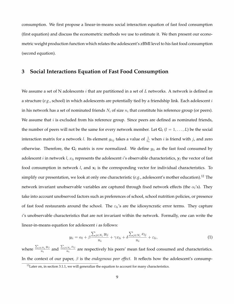
We assume a set of N adolescents i that are partitioned in a set of L networks. A network is defined as

a structure (e.g., school) in which adolescents are potentially tied by a friendship link. Each adolescent i

in his network has a set of nominated friends Ni of size ni that constitute his reference group (or peers).

We assume that i is excluded from his reference group. Since peers are defined as nominated friends,

the number of peers will not be the same for every network member. Let Gl (l = 1, . . . , L) be the social

interaction matrix for a network l. Its element glij takes a value of 1ni

when i is friend with j, and zero

otherwise. Therefore, the Gl matrix is row normalized. We define yli as the fast food consumed by

adolescent i in network l, xli represents the adolescent i’s observable characteristics, yl the vector of fast

food consumption in network l, and xl is the corresponding vector for individual characteristics. To

simplify our presentation, we look at only one characteristic (e.g., adolescent’s mother education).12 The

network invariant unobservable variables are captured through fixed network effects (the αl’s). They

take into account unobserved factors such as preferences of school, school nutrition policies, or presence

of fast food restaurants around the school. The εli’s are the idiosyncratic error terms. They capture

i’s unobservable characteristics that are not invariant within the network. Formally, one can write the

linear-in-means equation for adolescent i as follows:

yli = αl + β

∑j∈Ni

ylj

ni+ γxli + δ

∑j∈Ni

xlj

ni+ εli, (1)

where∑

j∈Niylj

niand

∑j∈Ni

xlj

niare respectively his peers’ mean fast food consumed and characteristics.

In the context of our paper, β is the endogenous peer effect. It reflects how the adolescent’s consump-12Later on, in section 3.1.1, we will generalize the equation to account for many characteristics.

9

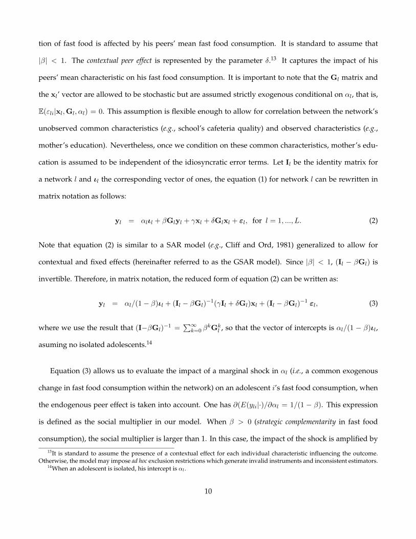
tion of fast food is affected by his peers’ mean fast food consumption. It is standard to assume that

|β| < 1. The contextual peer effect is represented by the parameter δ.13 It captures the impact of his

peers’ mean characteristic on his fast food consumption. It is important to note that the Gl matrix and

the xl’ vector are allowed to be stochastic but are assumed strictly exogenous conditional on αl, that is,

E(εli|xl,Gl, αl) = 0. This assumption is flexible enough to allow for correlation between the network’s

unobserved common characteristics (e.g., school’s cafeteria quality) and observed characteristics (e.g.,

mother’s education). Nevertheless, once we condition on these common characteristics, mother’s edu-

cation is assumed to be independent of the idiosyncratic error terms. Let Il be the identity matrix for

a network l and ιl the corresponding vector of ones, the equation (1) for network l can be rewritten in

matrix notation as follows:

yl = αlιl + βGlyl + γxl + δGlxl + εl, for l = 1, ..., L. (2)

Note that equation (2) is similar to a SAR model (e.g., Cliff and Ord, 1981) generalized to allow for

contextual and fixed effects (hereinafter referred to as the GSAR model). Since |β| < 1, (Il − βGl) is

invertible. Therefore, in matrix notation, the reduced form of equation (2) can be written as:

yl = αl/(1− β)ιl + (Il − βGl)−1(γIl + δGl)xl + (Il − βGl)

−1 εl, (3)

where we use the result that (I−βGl)−1 =

∑∞k=0 β

kGkl , so that the vector of intercepts is αl/(1 − β)ιl,

asuming no isolated adolescents.14

Equation (3) allows us to evaluate the impact of a marginal shock in αl (i.e., a common exogenous

change in fast food consumption within the network) on an adolescent i’s fast food consumption, when

the endogenous peer effect is taken into account. One has ∂(E(yli|·)/∂αl = 1/(1 − β). This expression

is defined as the social multiplier in our model. When β > 0 (strategic complementarity in fast food

consumption), the social multiplier is larger than 1. In this case, the impact of the shock is amplified by

13It is standard to assume the presence of a contextual effect for each individual characteristic influencing the outcome.Otherwise, the model may impose ad hoc exclusion restrictions which generate invalid instruments and inconsistent estimators.

14When an adolescent is isolated, his intercept is αl.

10

social interactions as more fast food consumption by his peers induces an adolescent to adopt a similar

behaviour.

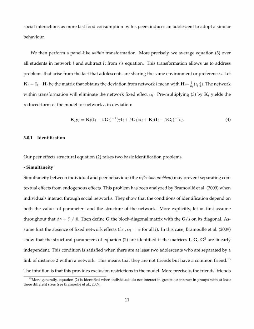
We then perform a panel-like within transformation. More precisely, we average equation (3) over

all students in network l and subtract it from i’s equation. This transformation allows us to address

problems that arise from the fact that adolescents are sharing the same environment or preferences. Let

Kl = Il−Hl be the matrix that obtains the deviation from network l mean with Hl=1nl

(ιlι′l). The network

within transformation will eliminate the network fixed effect αl. Pre-multiplying (3) by Kl yields the

reduced form of the model for network l, in deviation:

Klyl = Kl(Il − βGl)−1(γIl + δGl)xl + Kl(Il − βGl)

−1εl. (4)

3.0.1 Identification

Our peer effects structural equation (2) raises two basic identification problems.

- Simultaneity

Simultaneity between individual and peer behaviour (the reflection problem) may prevent separating con-

textual effects from endogenous effects. This problem has been analyzed by Bramoulle et al. (2009) when

individuals interact through social networks. They show that the conditions of identification depend on

both the values of parameters and the structure of the network. More explicitly, let us first assume

throughout that βγ + δ 6= 0. Then define G the block-diagonal matrix with the Gl’s on its diagonal. As-

sume first the absence of fixed network effects (i.e., αl = α for all l). In this case, Bramoulle et al. (2009)

show that the structural parameters of equation (2) are identified if the matrices I, G, G2 are linearly

independent. This condition is satisfied when there are at least two adolescents who are separated by a

link of distance 2 within a network. This means that they are not friends but have a common friend.15

The intuition is that this provides exclusion restrictions in the model. More precisely, the friends’ friends

15More generally, equation (2) is identified when individuals do not interact in groups or interact in groups with at leastthree different sizes (see Bramoulle et al., 2009).

11

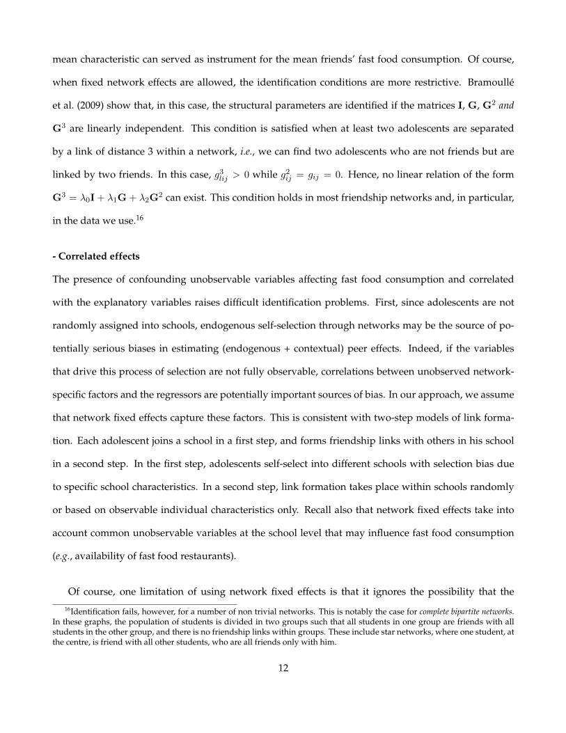
mean characteristic can served as instrument for the mean friends’ fast food consumption. Of course,

when fixed network effects are allowed, the identification conditions are more restrictive. Bramoulle

et al. (2009) show that, in this case, the structural parameters are identified if the matrices I, G, G2 and

G3 are linearly independent. This condition is satisfied when at least two adolescents are separated

by a link of distance 3 within a network, i.e., we can find two adolescents who are not friends but are

linked by two friends. In this case, g3lij > 0 while g2ij = gij = 0. Hence, no linear relation of the form

G3 = λ0I + λ1G + λ2G2 can exist. This condition holds in most friendship networks and, in particular,

in the data we use.16

- Correlated effects

The presence of confounding unobservable variables affecting fast food consumption and correlated

with the explanatory variables raises difficult identification problems. First, since adolescents are not

randomly assigned into schools, endogenous self-selection through networks may be the source of po-

tentially serious biases in estimating (endogenous + contextual) peer effects. Indeed, if the variables

that drive this process of selection are not fully observable, correlations between unobserved network-

specific factors and the regressors are potentially important sources of bias. In our approach, we assume

that network fixed effects capture these factors. This is consistent with two-step models of link forma-

tion. Each adolescent joins a school in a first step, and forms friendship links with others in his school

in a second step. In the first step, adolescents self-select into different schools with selection bias due

to specific school characteristics. In a second step, link formation takes place within schools randomly

or based on observable individual characteristics only. Recall also that network fixed effects take into

account common unobservable variables at the school level that may influence fast food consumption

(e.g., availability of fast food restaurants).

Of course, one limitation of using network fixed effects is that it ignores the possibility that the

16Identification fails, however, for a number of non trivial networks. This is notably the case for complete bipartite networks.In these graphs, the population of students is divided in two groups such that all students in one group are friends with allstudents in the other group, and there is no friendship links within groups. These include star networks, where one student, atthe centre, is friend with all other students, who are all friends only with him.

12

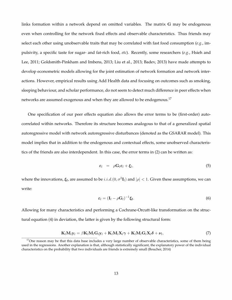
links formation within a network depend on omitted variables. The matrix G may be endogenous

even when controlling for the network fixed effects and observable characteristics. Thus friends may

select each other using unobservable traits that may be correlated with fast food consumption (e.g., im-

pulsivity, a specific taste for sugar- and fat-rich food, etc). Recently, some researchers (e.g., Hsieh and

Lee, 2011; Goldsmith-Pinkham and Imbens, 2013; Liu et al., 2013; Badev, 2013) have made attempts to

develop econometric models allowing for the joint estimation of network formation and network inter-

actions. However, empirical results using Add Health data and focusing on outcomes such as smoking,

sleeping behaviour, and scholar performance, do not seem to detect much difference in peer effects when

networks are assumed exogenous and when they are allowed to be endogenous.17

One specification of our peer effects equation also allows the error terms to be (first-order) auto-

correlated within networks. Therefore its structure becomes analogous to that of a generalized spatial

autoregressive model with network autoregressive disturbances (denoted as the GSARAR model). This

model implies that in addition to the endogenous and contextual effects, some unobserved characteris-

tics of the friends are also interdependent. In this case, the error terms in (2) can be written as:

εl = ρGlεl + ξl, (5)

where the innovations, ξl, are assumed to be i.i.d.(0, σ2Il) and |ρ| < 1. Given these assumptions, we can

write:

εl = (Il − ρGl)−1ξl. (6)

Allowing for many characteristics and performing a Cochrane-Orcutt-like transformation on the struc-

tural equation (4) in deviation, the latter is given by the following structural form:

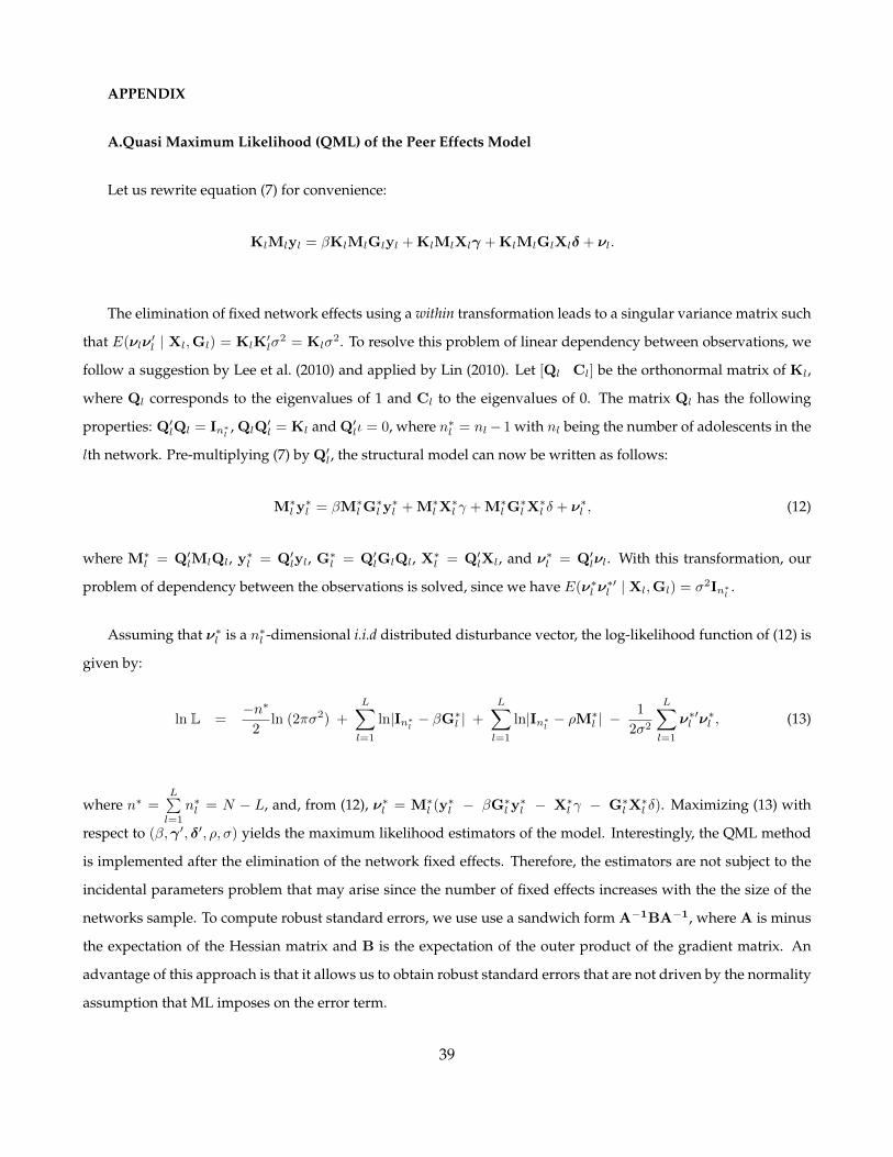
KlMlyl = βKlMlGlyl + KlMlXlγ + KlMlGlXlδ + νl, (7)17One reason may be that this data base includes a very large number of observable characteristics, some of them being

used in the regressions. Another explanation is that, although statistically significant, the explanatory power of the individualcharacteristics on the probability that two individuals are friends is extremely small (Boucher, 2014)

13

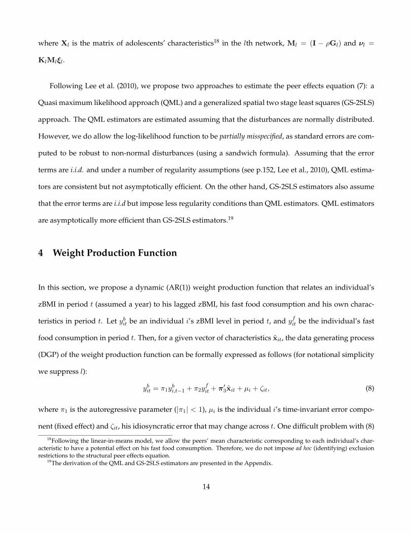
where Xl is the matrix of adolescents’ characteristics18 in the lth network, Ml = (I − ρGl) and νl =

KlMlξl.

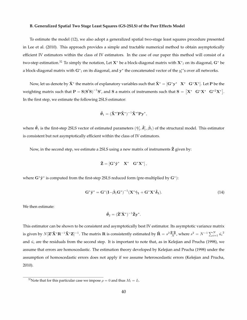
Following Lee et al. (2010), we propose two approaches to estimate the peer effects equation (7): a

Quasi maximum likelihood approach (QML) and a generalized spatial two stage least squares (GS-2SLS)

approach. The QML estimators are estimated assuming that the disturbances are normally distributed.

However, we do allow the log-likelihood function to be partially misspecified, as standard errors are com-

puted to be robust to non-normal disturbances (using a sandwich formula). Assuming that the error

terms are i.i.d. and under a number of regularity assumptions (see p.152, Lee et al., 2010), QML estima-

tors are consistent but not asymptotically efficient. On the other hand, GS-2SLS estimators also assume

that the error terms are i.i.d but impose less regularity conditions than QML estimators. QML estimators

are asymptotically more efficient than GS-2SLS estimators.19

4 Weight Production Function

In this section, we propose a dynamic (AR(1)) weight production function that relates an individual’s

zBMI in period t (assumed a year) to his lagged zBMI, his fast food consumption and his own charac-

teristics in period t. Let ybit be an individual i’s zBMI level in period t, and yfit be the individual’s fast

food consumption in period t. Then, for a given vector of characteristics xit, the data generating process

(DGP) of the weight production function can be formally expressed as follows (for notational simplicity

we suppress l):

ybit = π1ybi,t−1 + π2y

fit + π′3xit + µi + ζit, (8)

where π1 is the autoregressive parameter (|π1| < 1), µi is the individual i’s time-invariant error compo-

nent (fixed effect) and ζit, his idiosyncratic error that may change across t. One difficult problem with (8)

18Following the linear-in-means model, we allow the peers’ mean characteristic corresponding to each individual’s char-acteristic to have a potential effect on his fast food consumption. Therefore, we do not impose ad hoc (identifying) exclusionrestrictions to the structural peer effects equation.

19The derivation of the QML and GS-2SLS estimators are presented in the Appendix.

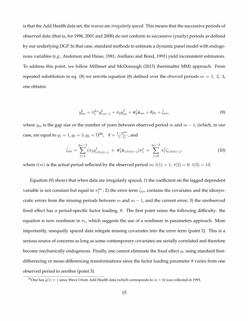
14

is that the Add Health data set, the waves are irregularly spaced. This means that the successive periods of

observed data (that is, for 1996, 2001 and 2008) do not conform to successive (yearly) periods as defined

by our underlying DGP. In that case, standard methods to estimate a dynamic panel model with endoge-

nous variables (e.g., Anderson and Hsiao, 1981; Arellano and Bond, 1991) yield inconsistent estimators.

To address this point, we follow Millimet and McDonough (2013) (hereinafter MM) approach. From

repeated substitution in eq. (8) we rewrite equation (8) defined over the observed periods m = 1, 2, 3,

one obtains:

ybim = πgm1 ybi,m−1 + π2yfim + π′3xim + θµi + ζim, (9)

where gm is the gap size or the number of years between observed period m and m − 1, (which, in our

case, are equal to g1 = 1, g2 = 5, g3 = 7)20; θ =1−πgm

11−π1 , and

ζim =

gm−1∑j=1

(π2yfi,t(m)−j + π′3xi,t(m)−j)π

j1 +

gm−1∑j=0

πj1ζi,t(m)−j , (10)

where t(m) is the actual period reflected by the observed period m: t(1) = 1; t(2) = 6; t(3) = 13.

Equation (9) shows that when data are irregularly spaced, 1) the coefficient on the lagged dependent

variable is not constant but equal to πgm1 ; 2) the error term ζim contains the covariates and the idiosyn-

cratic errors from the missing periods between m and m − 1, and the current error; 3) the unobserved

fixed effect has a period-specific factor loading, θ. The first point raises the following difficulty: the

equation is now nonlinear in π1, which suggests the use of a nonlinear in parameters approach. More

importantly, unequally spaced data relegate missing covariates into the error term (point 2). This is a

serious source of concerns as long as some contemporary covariates are serially correlated and therefore

become mechanically endogenous. Finally, one cannot eliminate the fixed effect µi using standard first-

differencing or mean-differencing transformations since the factor loading parameter θ varies from one

observed period to another (point 3).

20One has g(1) = 1 since Wave I from Add Health data (which corresponds to m = 0) was collected in 1995.

15

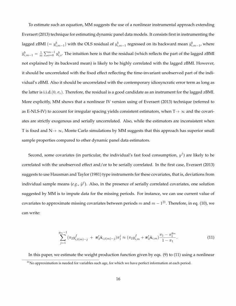
To estimate such an equation, MM suggests the use of a nonlinear instrumental approach extending

Everaert (2013) technique for estimating dynamic panel data models. It consists first in instrumenting the

lagged zBMI (= ybi,m−1) with the OLS residual of ybi,m−1 regressed on its backward mean ybi,m−1, where

ybi,m−1 = 1m

∑m−1s=0 ybi,s. The intuition here is that the residual (which reflects the part of the lagged zBMI

not explained by its backward mean) is likely to be highly correlated with the lagged zBMI. However,

it should be uncorrelated with the fixed effect reflecting the time-invariant unobserved part of the indi-

vidual’s zBMI. Also it should be uncorrelated with the contemporary idiosyncratic error term as long as

the latter is i.i.d.(0, σε). Therefore, the residual is a good candidate as an instrument for the lagged zBMI.

More explicitly, MM shows that a nonlinear IV version using of Everaert (2013) technique (referred to

as E-NLS-IV) to account for irregular spacing yields consistent estimators, when T→ ∞ and the covari-

ates are strictly exogenous and serially uncorrelated. Also, while the estimators are inconsistent when

T is fixed and N→ ∞, Monte Carlo simulations by MM suggests that this approach has superior small

sample properties compared to other dynamic panel data estimators.

Second, some covariates (in particular, the individual’s fast food consumption, yf ) are likely to be

correlated with the unobserved effect and/or to be serially correlated. In the first case, Everaert (2013)

suggests to use Hausman and Taylor (1981) type instruments for these covariates, that is, deviations from

individual sample means (e.g., yf ). Also, in the presence of serially correlated covariates, one solution

suggested by MM is to impute data for the missing periods. For instance, we can use current value of

covariates to approximate missing covariates between periods m and m− 121. Therefore, in eq. (10), we

can write:

gm−1∑j=1

(π2yfi,t(m)−j + π′3xi,t(m)−j)π

j1 ≈ (π2y

fi,m + π′3xi,m)

π1 − πgm11− π1

. (11)

In this paper, we estimate the weight production function given by eqs. (9) to (11) using a nonlinear

21No approximation is needed for variables such age, for which we have perfect information at each period.

16

instrumental approach and based on current values of covariates to approximate missing data for the

missing periods. Following MM, we denote this estimator: E-NLS-IV-C. We also present a GMM version

of this estimator using a two-step approach to obtain an optimal weighting matrix (clustered at the

individual level).

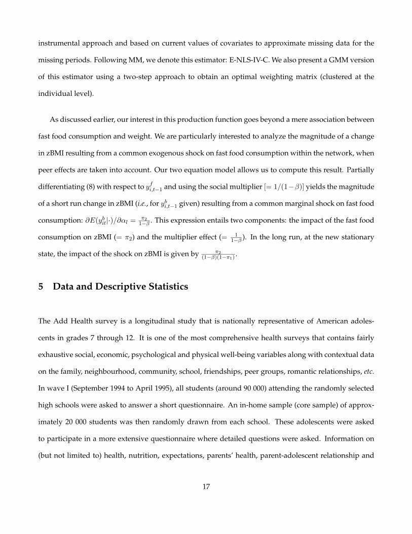
As discussed earlier, our interest in this production function goes beyond a mere association between

fast food consumption and weight. We are particularly interested to analyze the magnitude of a change

in zBMI resulting from a common exogenous shock on fast food consumption within the network, when

peer effects are taken into account. Our two equation model allows us to compute this result. Partially

differentiating (8) with respect to yfi,t−1 and using the social multiplier [= 1/(1−β)] yields the magnitude

of a short run change in zBMI (i.e., for ybi,t−1 given) resulting from a common marginal shock on fast food

consumption: ∂E(ybit|·)/∂αl = π21−β . This expression entails two components: the impact of the fast food

consumption on zBMI (= π2) and the multiplier effect (= 11−β ). In the long run, at the new stationary

state, the impact of the shock on zBMI is given by π2(1−β)(1−π1) .

5 Data and Descriptive Statistics

The Add Health survey is a longitudinal study that is nationally representative of American adoles-

cents in grades 7 through 12. It is one of the most comprehensive health surveys that contains fairly

exhaustive social, economic, psychological and physical well-being variables along with contextual data

on the family, neighbourhood, community, school, friendships, peer groups, romantic relationships, etc.

In wave I (September 1994 to April 1995), all students (around 90 000) attending the randomly selected

high schools were asked to answer a short questionnaire. An in-home sample (core sample) of approx-

imately 20 000 students was then randomly drawn from each school. These adolescents were asked

to participate in a more extensive questionnaire where detailed questions were asked. Information on

(but not limited to) health, nutrition, expectations, parents’ health, parent-adolescent relationship and

17

friends nomination was gathered.22 This cohort was then followed in-home in the subsequent waves in

1996 (wave II), 2001 (wave III) and 2008-2009 (wave IV). The extensive questionnaire was also used to

construct the saturation sample that focuses on 16 selected schools (about 3000 students). Every student

attending these selected schools answered the detailed questionnaire. There are two large schools and

14 other small schools. All schools are racially mixed and are located in major metropolitan areas except

one large school that has a high concentration of white adolescents and is located in a rural area. Con-

sequently, fast food consumption may be subject to downward bias if one accepts the argument that the

fast food consumption among white adolescents is usually lower than that of black adolescents.

In this paper we use the saturation sample of wave II in-home survey to investigate the presence of

peer effects in fast food consumption.23 One of the innovative aspects of this wave is the introduction

of the nutrition section. It reports among other things food consumption variables (e.g., fast food, soft

drinks, desserts, etc.). This allows us to depict food consumption patterns of each adolescent and re-

late it to that of his peer group. In addition, the availability of friend nomination allows us to retrace

school friends and thus construct friendship networks. To estimate the weight production function, we

considered information from wave I, wave II, wave III and wave IV.

We exploit friends nominations to construct the network of friends. Thus, we consider all nominated

friends as network members regardless of the reciprocity of the nomination. If an adolescent nominates

a friend then a link is assigned between these two adolescents (directed network with non symmetric

links).22Adolescents were asked to nominate up to five female friends and five male friends.23It includes all meals that are consumed at a fast food restaurant such as McDonald’s, Burger King, Pizza Hut, Taco Bell

and other fast food outlets.

18

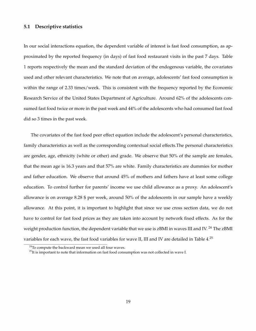
5.1 Descriptive statistics

In our social interactions equation, the dependent variable of interest is fast food consumption, as ap-

proximated by the reported frequency (in days) of fast food restaurant visits in the past 7 days. Table

1 reports respectively the mean and the standard deviation of the endogenous variable, the covariates

used and other relevant characteristics. We note that on average, adolescents’ fast food consumption is

within the range of 2.33 times/week. This is consistent with the frequency reported by the Economic

Research Service of the United States Department of Agriculture. Around 62% of the adolescents con-

sumed fast food twice or more in the past week and 44% of the adolescents who had consumed fast food

did so 3 times in the past week.

The covariates of the fast food peer effect equation include the adolescent’s personal characteristics,

family characteristics as well as the corresponding contextual social effects.The personal characteristics

are gender, age, ethnicity (white or other) and grade. We observe that 50% of the sample are females,

that the mean age is 16.3 years and that 57% are white. Family characteristics are dummies for mother

and father education. We observe that around 45% of mothers and fathers have at least some college

education. To control further for parents’ income we use child allowance as a proxy. An adolescent’s

allowance is on average 8.28 $ per week, around 50% of the adolescents in our sample have a weekly

allowance. At this point, it is important to highlight that since we use cross section data, we do not

have to control for fast food prices as they are taken into account by network fixed effects. As for the

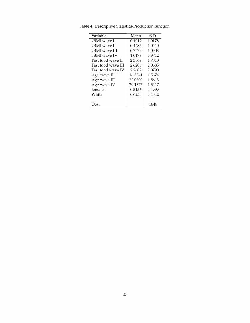
weight production function, the dependent variable that we use is zBMI in waves III and IV. 24 The zBMI

variables for each wave, the fast food variables for wave II, III and IV are detailed in Table 4.25

24To compute the backward mean we used all four waves.25It is important to note that information on fast food consumption was not collected in wave I.

19

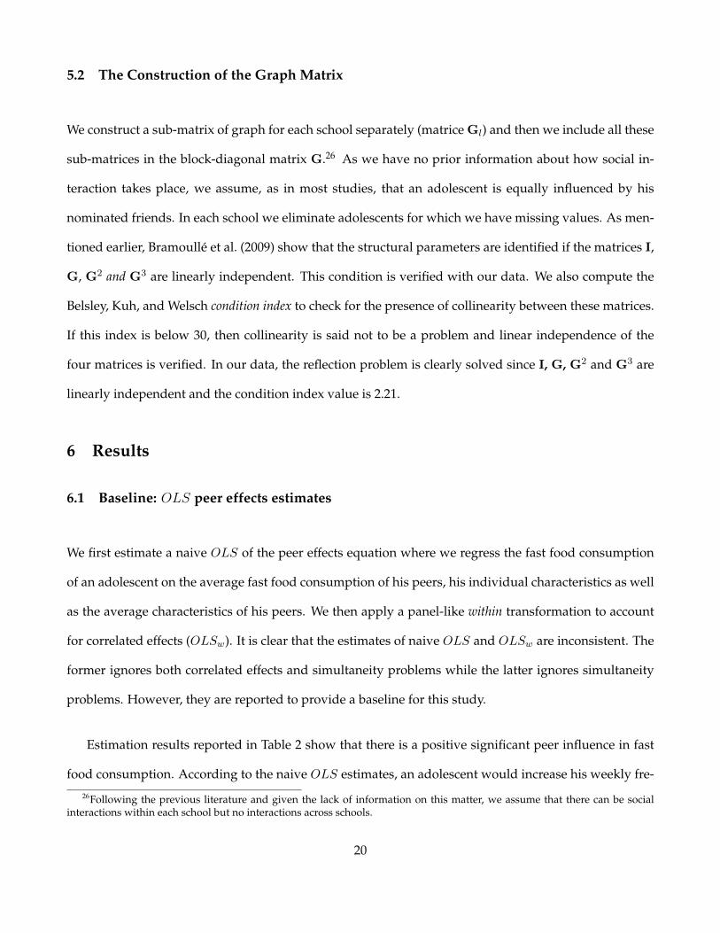
5.2 The Construction of the Graph Matrix

We construct a sub-matrix of graph for each school separately (matrice Gl) and then we include all these

sub-matrices in the block-diagonal matrix G.26 As we have no prior information about how social in-

teraction takes place, we assume, as in most studies, that an adolescent is equally influenced by his

nominated friends. In each school we eliminate adolescents for which we have missing values. As men-

tioned earlier, Bramoulle et al. (2009) show that the structural parameters are identified if the matrices I,

G, G2 and G3 are linearly independent. This condition is verified with our data. We also compute the

Belsley, Kuh, and Welsch condition index to check for the presence of collinearity between these matrices.

If this index is below 30, then collinearity is said not to be a problem and linear independence of the

four matrices is verified. In our data, the reflection problem is clearly solved since I, G, G2 and G3 are

linearly independent and the condition index value is 2.21.

6 Results

6.1 Baseline: OLS peer effects estimates

We first estimate a naive OLS of the peer effects equation where we regress the fast food consumption

of an adolescent on the average fast food consumption of his peers, his individual characteristics as well

as the average characteristics of his peers. We then apply a panel-like within transformation to account

for correlated effects (OLSw). It is clear that the estimates of naive OLS and OLSw are inconsistent. The

former ignores both correlated effects and simultaneity problems while the latter ignores simultaneity

problems. However, they are reported to provide a baseline for this study.

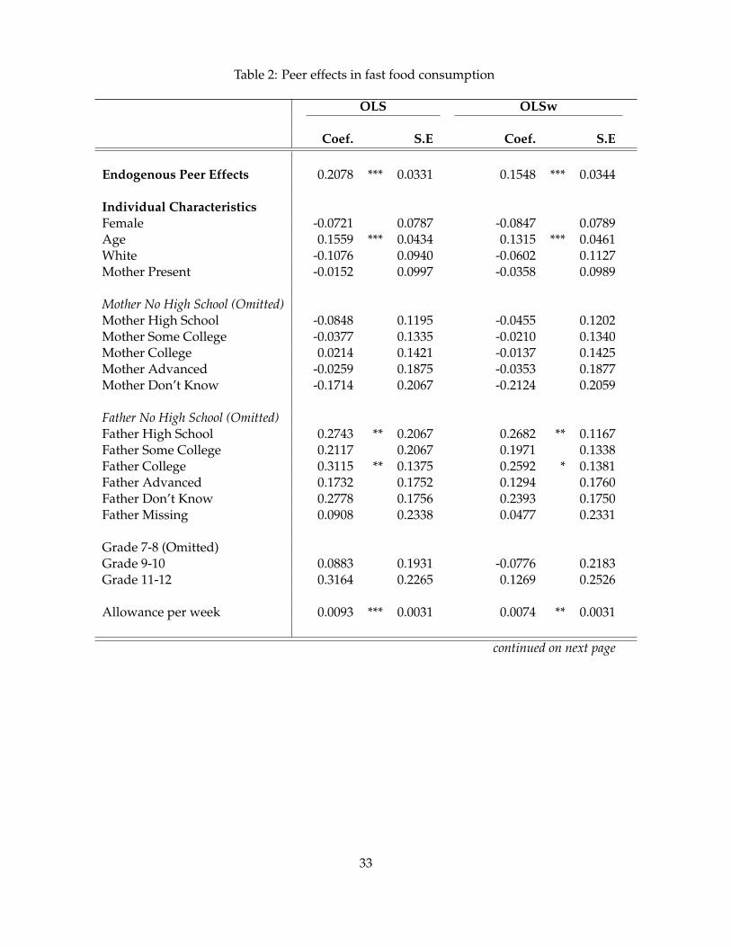
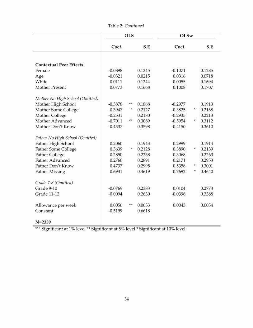
Estimation results reported in Table 2 show that there is a positive significant peer influence in fast

food consumption. According to the naive OLS estimates, an adolescent would increase his weekly fre-

26Following the previous literature and given the lack of information on this matter, we assume that there can be socialinteractions within each school but no interactions across schools.

20

quency (in days) of fast food restaurant visits by 0.21 in response to an extra day of fast food restaurant

visits by his friends. On average, this corresponds to an increase of 9% (= 0.21/2.33). OLSw estimate is

slightly lower (= 0.15, or 6.6%). This reduction in the estimated effect may partly be explained by the

fact that adolescents in the same reference group tend to choose a similar level of fast food consump-

tion partly because they face a common environment or because adolescents with similar characteristics

tend to attend the same school (homophily). As for the individual characteristics, age, father education

and weekly allowance positively affect fast food consumption. Turning our attention to the contextual

peer effects, we notice that the latter variable decreases with mean peers’ mother’s education and in-

creases with mean peers’ father’s education. The former result indicates that friends’ mother education

negatively affects an adolescent’s fast food consumption.

6.2 GS-2SLS and QML peer effects estimates

Next, we estimate our peer effects equation with school fixed effects using GS-2SLS (with i.i.d. error

terms and without imposing autoregressive disturbances: ρ = 0). We then estimate this equation using

a QML approach with i.i.d. error terms . Also, we estimate another plausible version of this model by

allowing network autoregressive disturbances (GSARAR model).

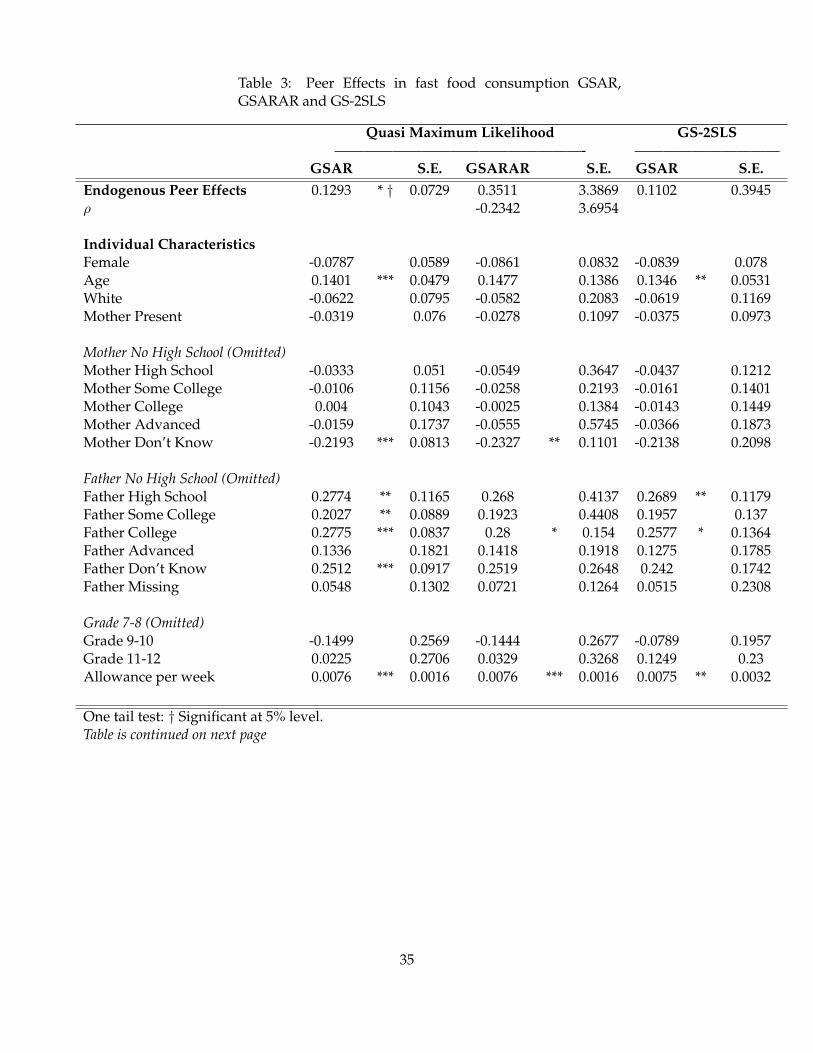
Estimation results are displayed in Table 3. The GS-2SLS approach (see last two columns) assumes

that the instrument for G∗y∗ is given by G∗y∗ (see eq. 14).27 One can check whether this instrument

is weak by regressing G∗y∗ on G∗y∗, X∗ and G∗X∗ and performing a Stock-Yogo test (see Table 3).

It consists in comparing the Cragg-Donald F statistic associated with the estimated coefficient of G∗y∗

(= 17.80) with its critical value when one assumes a 10% tolerance28 for the size distortion of the 5% Wald

test (= 16.38). Based on this test, we reject that the instrument is weak. The endogenous effect resulting

from GS-2SLS estimation is positive (=0.11 or 4.73%) but non significant. When using the GSAR QML

27The star superscript indicates that the original variable has been transformed to eliminate the problem of singular variancematrix generated by the use of the within transformation to eliminate fixed network effects. See Appendix.

28This level of tolerance is the smallest one that can be computed given that there is only one excluded instrument.

21

approach, estimation results show a positive endogenous effect of 0.129 (or 5.3%). This estimate reveals

to be very close to the one obtained by GS-2SLS and is slightly smaller than the OLS ones obtained in

the previous sub-section. It is statistically significant at the 5% level if we perform a one tail test (one-tail

p value = 0,039) but at 10% if we consider a two-tail test (two tail p value= 0.0785). While this result

suggests that one has to be quite cautious when accepting the estimate, it can be argued that one should

perform a one-tail test since one expects the endogenous peer effect to be either positive or zero. In that

case, the social multiplier associated with an exogenous increase in an adolescent fast food consumption

is 1.15 (= 11−0.129 ) and is significantly different from 1 at the 10% level, based on a one-tail test (its

standard error is 0.096 using the delta method, with a one-tail p-value of 0.059). This reflects a relatively

low endogenous peer effect.

How can we compare these results to those obtained previously in the related literature? Although

there are few studies that investigated the presence of peer effects in fast food consumption using the

linear-in-means equation , a richer body of literature has investigated a tangent issue : obesity. As com-

pared with endogenous effects obtained in the literature on obesity, our peer effect is intermediate be-

tween studies that obtain no peer effects (Cohen-Cole and Fletcher, 2008b) and the literature that provides

evidence that there are peer effects are strong, for instance, generating a social multiplier larger than 1.5

(e.g., Christakis and Fowler, 2007; Trogdon et al., 2008).29

To check the sensitivity of these results to the presence of SAR disturbances, we also estimate our

model using a GSARAR QML specification. The estimated spatial autocorrelation coefficient is negative

but not significant at the 5% level. Moreover the endogenous peer effect is large (=0.3655) but no longer

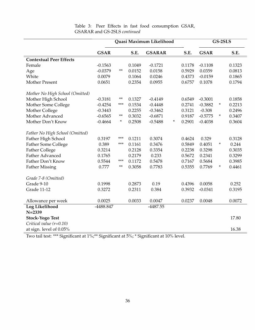
significant even at the 10% level (one-tail test). Also a likelihood test does not reject the GSAR QML spec-

ification. Therefore we consider the latter as our preferred one. This suggests a much lower endogenous

peer effect (= 0.13), which can be interpreted as a lower bound to this parameter, at least when assuming

29More specifically, Cohen-Cole and Fletcher (2008b) finds a statistically insignificant social multiplier of 1.03, Christakisand Fowler (2007) find a statistically significant social multiplier of 2.63 and Trogdon et al. (2008) find a statistically significantsocial multiplier of 2.08.

22

that selection on unobservables is not an important source of biases, after controlling for network fixed

effects and observable characteristics (see our discussion above).

To sum up, we can say that results in general are consistent with the hypothesis that fast food con-

sumption is linked to issues of interactions with friends. However, our social multiplier estimate does

not appear to be very strong (as the endogenous effects are less than 0.3), at least when we consider

a specification which seems reasonable. This result, despite its small magnitude, addresses the puzzle

around the behavioural channels through which peer effects in weight gain flows. Indeed, while Yaku-

sheva et al. (2014) in their attempt to uncover the channels through which these effects flow have tested

for two behavioural channels exercise and eating disorders (e.g., anorexia), they could not test for the

presence of peer effects in eating habits due to data limitations.

As for estimated individual effects and focusing on the GSAR QML specification, they follow fairly

the baseline model. Fast food consumption is positively associated with age and father’s education as

well as positively associated with weekly allowance. Mother’s education seems to have a negative but

non significant impact on fast food consumption. It is important to note that while the general perception

is that fast food is an inferior good, the empirical evidence suggests a positive income elasticity (Aguiar

and Hurst, 2005). The positive relation between fast food consumption and allowance is thus in line with

the positive relation between income and fast food consumption.

One advantage of our spatial approach is that it allows to identify both endogenous and contex-

tual peer effects. Turning our attention to the latter, we note in particular that an adolescent’s fast food

consumption decreases with peers’ mother’s education but increases with mean peers’ father’s educa-

tion. While the former causal effect seems natural as mothers with higher education may (directly and

indirectly) encourage both their children and their friends to have better eating habits, the latter effect

is rather puzzling. One partial explanation is that fathers with higher education are more likely to be

absent from home. Therefore they have less positive influence on their children’s and friends’ eating

23

habits.

6.3 Weight production function estimates

Estimation results presented in the earlier sections are consistent with the presence of peer effects in

fast food consumption. Nevertheless, we still need to provide evidence of the presence of a relation-

ship between fast food consumption and weight gain. In this section we report estimates of the weight

production function presented earlier.

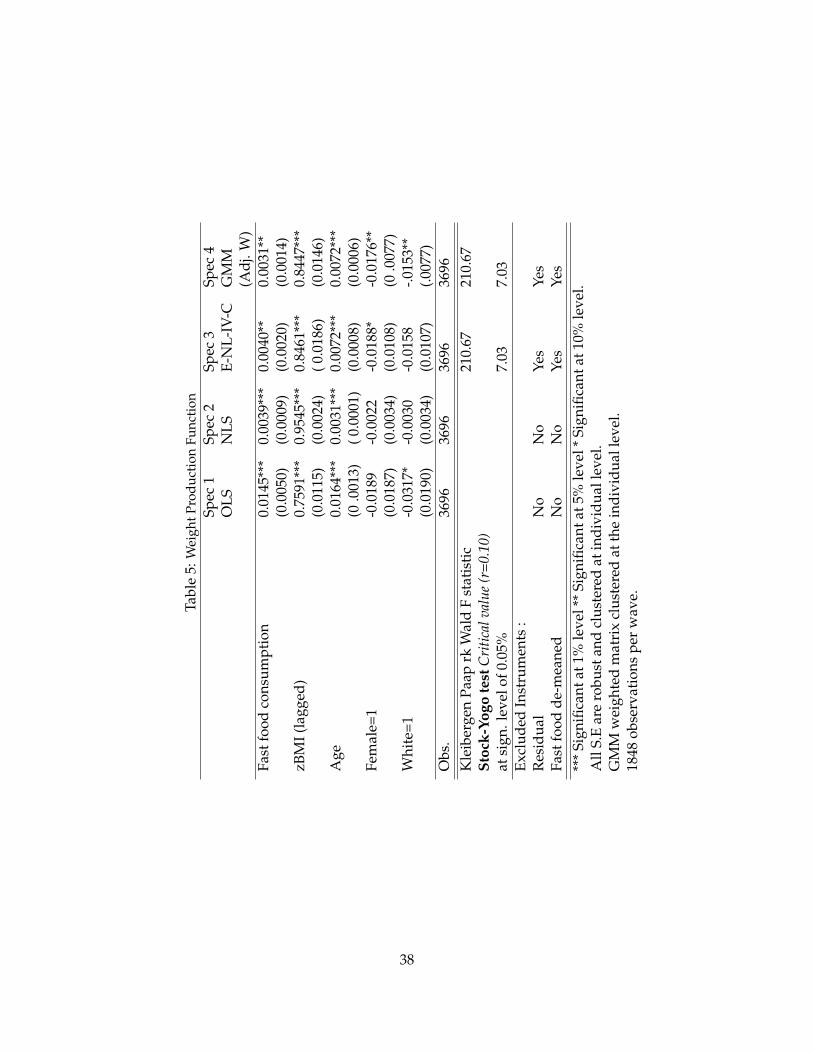
Results from the estimation of the production function are reported in Table 5. Specification (1)

shows baseline OLS estimates of equation (8) (where t is replaced by m), specification (2) shows the

NLS estimates of equation (9), specification (3) shows E-NL-IV-C estimation results for equation (9) and

finally specification (4) shows GMM version the previous estimator using a two step with an optimal

weighting matrix. All specifications are estimated using wave 3 and wave 4, but where information

from wave 1 and wave 2 are used to construct the instruments.

In line with our expectations, the general results indicate that lagged zBMI and current fast food

consumption have positive significant effect (which is between 0 and 1, in the case of the lagged zBMI)

on current zBMI. These results seem to be robust across different specifications with some differences

that can be explained by the differences in the assumptions made on the DGP. More specifically results in

specification (1), our baseline specification, are comparable to previous findings by Niemeier et al. (2006)

who used the same data set. The impact of lagged zBMI is 0.7591 (compared to 0.7600 for Niemeier et al.

(2006)). As for the impact of fast food consumption, it is 0.014 (compared to 0.020 for Niemeier et al.

(2006)). 30

Comparing specification (1) with specification (2), we notice that the estimate of the fast food con-

sumption marginal effect is much higher in the former than in the latter case (0.0145 vs. 0.0039). The

30It is important to note that Niemeier et al. (2006) used a different wave and a different approach.

24

basic explanation is that when estimating the parameter π2 in the specification (1), we are not accounting

for missing data on yfit in time intervals between m and m−1. In fact, we are estimating π2(1−πgm

11−π1

), with

(1−πgm

11−π1

)> 1, instead of estimating π2. Also the estimate associated with the lagged endogenous variable

is smaller in specification (1) than in specification (2) (i.e., 0.7591 vs. 0.9545). The explanation is that in

the OLS specification we are implicitly estimating πgm1 with |π1| < 1 as we are ignoring the irregularly

time intervals.

While specification (2) accounts for the unequally spaced intervals, it does not account for the corre-

lation between lagged zBMI and the time-invariant unobserved effect and the idiosyncratic error term

of zBMI. Further it does take into account the fact that fast food consumption may be correlated with

the time-invariant unobserved effect. To account for these possibilities, we follow MM and instrument

zBMI using the OLS residuals of the regression lagged zBMI on its backward mean. As for the fast food

consumption, it is instrumented using Hausman and Taylor (1981) type of instruments, that is, by taking

the deviations of fast food consumption with respect to individual sample mean as an instrument.

The estimation of specification (3) shows results that are consistent with previous results, with some

differences in the magnitude of the parameters. The estimated parameter associated with zBMI is smaller

than the one obtained in the second specification (0.8461 vs. 0.9545). As for the estimated parameter

for fast food consumption it is marginally higher when using E-NL-IV-C (0.0040 vs. 0.0039). All results

remain statistically significant. To complement results from the E-NL-IV-C we estimate an optimal GMM

version (with a weighted matrix clustered at the the individual level) of the same model. Estimation

results are again within the expected lines and consistent with previous estimates with some variation

in the estimates of the lagged zBMI (0.8447 vs. 0.8461) and fast food consumption parameters (0.0039 vs.

0.0031).

We retain specification (4) as our preferred one as it provide optimal and robust estimators. Results

from this specification show that lagged zBMI has a positive significant effect on current zBMI level (=

25

0.8447). This suggests that an exogenous shock on weight has a stronger effect in the long term than in

the short term. Based on specification (4), an extra day of fast food restaurant visit per week increases

zBMI by 0.02 (= 0.00311−0.8447 ) zBMI points or 4.45% in the long term. The presence of a causal link between

fast food consumption and zBMI does not come as a surprise since previous findings have been pointing

in this direction (e.g., Levitsky et al., 2004; Niemeier et al., 2006; Rosenheck, 2008). Combining the impact

of fast food on weight gain with the social multiplier, our results suggest that an extra day of fast food

restaurant visits per week leads to a zBMI increase of 0.0351 zBMI points, or 5.11% (= 4.45% × 1.15) on

average, as compared with 4.45% with no peer effects. These results highlight a role for peer effects in

fast food consumption as one transmission mechanism through which weight gain is amplified.

As for the other covariates, age reveals to have a positive significant effect on zBMI, an additional

year increasing zBMI by 0.0072 zBMI points. Also being female and white have a negative effect on

zBMI (respectively 0.0176 and 0.0153). To test for the relevance of the instruments we use Kleibergen-

Paap rank test (which is used here to take into account the fact that the estimated standard errors are

panel clustered). The test rejects the null hypothesis that the instruments are weak.31

7 Conclusion

This paper investigates whether peer effects in adolescent weight partly flow through the eating habits

channel. We first attempt to study the presence of significant endogenous peer effects in fast food con-

sumption. New methods based on spatial econometric analysis are used to identify and estimate our

model, under the assumption that individuals interact through a friendship social network. Our results

indicate that an increase in his friends’ mean fast food consumption induces an adolescent to increase

his own fast food consumption. This peer effect amplifies through a social multiplier the impact of any

exogenous shock on fast food consumption. However, our estimated social multiplier based on our

31As the model is exactly identified, it is not possible to conduct an over identification test.

26

preferred (conservative) specification is small as it is equal to 1.15.

We also estimate a dynamic weight production function which relates the individual’s Body Mass

Index to his fast food consumption. Our results reveal a positive significant impact of a change in fast

food consumption on the change in zBMI. Specifically, in the long run, a one-unit increase in the weekly

frequency (in days) of fast food consumption produces an increase in zBMI by 4.45%. This effect reaches

5.11% when the social multiplier is taken into account. This suggests the presence of a positive but low

endogenous peer effect. In short, our results are intermediate between studies on overweight or obesity

that report no peer effects (e.g., Cohen-Cole and Fletcher, 2008a) and others that provide evidence of

strong peer effects (e.g., Trogdon et al., 2008; Christakis and Fowler, 2007)

Coupled with the reduction in the relative price of fast food and the increasing availability of fast

food restaurants over time, the social multiplier could somewhat increase the prevalence of obesity in

the years to come. Conversely, this multiplier may contribute to the decline of the spread of obesity and

the decrease in health care costs, as long as it is exploited by policy makers through tax and subsidy

reforms encouraging adequate eating habits among adolescents, or used to implement network based

interventions to promote healthy eating behaviours (Fletcher et al., 2011).

There are many possible extensions to this paper. From a policy perspective, it would be interesting

to investigate the presence of peer effects in physical activity of adolescents. A recent study by Charness

and Gneezy (2009) finds that there is room for intervention in peoples’ decisions to perform physical

exercise through financial incentives. It would be thus valuable to investigate whether there is a social

multiplier that can be exploited to amplify these effects. Furthermore, in the same way, it would be

interesting to study the presence of peer effects weight perceptions. So far, most of the peer effects work

has focused mainly on BMI outcomes. At the methodological level, a possible extension would be to

assume a Poisson or a Negative Binomial distribution to account for the count nature of the consumption

data at hand. As far as we know, no work has been carried out in this area. Finally, it would be most

27

useful to develop a general approach that would allow same sex and opposite sex peer effects to be

different for both males and females.

References

Aguiar, M. and Hurst, E. (2005), ‘Consumption versus expenditure’, Journal of Political Economy113(5), 919–948.

Ali, M. M., Amialchuk, A. and Heiland, F. W. (2011), ‘Weight-related behavior among adolescents: Therole of peer effects’, PloS one 6(6), e21179.

Ali, M. M., Amialchuk, A. and Renna, F. (2011), ‘Social network and weight misperception among ado-lescents’, Southern Economic Journal 77(4), 827–842.

Alviola IV, P. A., Nayga Jr, R. M., Thomsen, M. R., Danforth, D. and Smartt, J. (2014), ‘The effect offast-food restaurants on childhood obesity: A school level analysis’, Economics & Human Biology12, 110–119.

Anderson, B., Lyon-Callo, S., Fussman, C., Imes, G. and Rafferty, A. P. (2011), ‘Peer reviewed: Fast-foodconsumption and obesity among michigan adults’, Preventing chronic disease 8(4).

Anderson, M. and Matsa, D. (2011), ‘Are restaurants really supersizing america?’, American EconomicJournal: Applied Economics 3(1), 152–188.

Anderson, T. and Hsiao, C. (1981), ‘Estimation of dynamic models with error components’, Journal of theAmerican Statistical Association 76, 598–606.

Arellano, M. and Bond, S. (1991), ‘Some tests of specification for panel data: Monte Carlo evidence andan application to employment equations’, The Review of Economic Studies 58(2), 277–297.

Auld, M. C. and Powell, L. M. (2009), ‘Economics of food energy density and adolescent body weight’,Economica 76(304), 719–740.

Badev, A. (2013), Discrete games in endogenous networks: Theory and policy, Working Papers 2-1-2013,University of Pennsylvania Scholarly Commons.

Berentzen, T., Petersen, L., Schnohr, P. and Sørensen, T. (2008), ‘Physical activity in leisure-time is notassociated with 10-year changes in waist circumference’, Scandinavian Journal of Medicine & Sciencein Sports 18(6), 719–727.

Bleich, S., Cutler, D., Murray, C. and Adams, A. (2008), ‘Why is the developed world obese?’, AnnualReview of Public health 29, 273–295.

Blume, L., Brock, W., Durlauf, S. and Jayaraman, R. (2015), ‘Linear social interactions models’, Journal ofPolitical Economy 123(2), 444–496.

Boucher, V. (2014), ‘Conformism and self-selection in social networks’, Mimeo .

Bramoulle, Y., Djebbari, H. and Fortin, B. (2009), ‘Identification of peer effects through social networks’,Journal of Econometrics 150(1), 41–55.

28

Calabr, P., Golia, E., Maddaloni, V., Malvezzi, M., Casillo, B., Marotta, C., Calabro, R. and Golino, P.(2009), ‘Adipose tissue-mediated inflammation: the missing link between obesity and cardiovascu-lar disease?’, Internal and Emergency Medicine 4(1), 25–34.

Calle, E. (2007), ‘Obesity and cancer’, British Medical Journal 335(7630), 1107–1108.

Caraher, M. and Cowburn, G. (2007), ‘Taxing food: implications for public health nutrition’, Public HealthNutrition 8(08), 1242–1249.

Charness, G. and Gneezy, U. (2009), ‘Incentives to exercise’, Econometrica 77(3), 909–931.

Christakis, N. A. and Fowler, J. H. (2013), ‘Social contagion theory: examining dynamic social networksand human behavior’, Statistics in Medicine 32(4), 556–577.

Christakis, N. and Fowler, J. (2007), ‘The spread of obesity in a large social network over 32 years’, NewEngland Journal of Medicine 357(4), 370–379.

Cliff, A. and Ord, J. (1981), Spatial processes: models & applications, Pion Ltd.

Cohen-Cole, E. and Fletcher, J. (2008a), ‘Detecting implausible social network effects in acne, height, andheadaches: longitudinal analysis’, BMJ 337, a2533.

Cohen-Cole, E. and Fletcher, J. (2008b), ‘Is obesity contagious?: social networks vs. environmental factorsin the obesity epidemic’, Journal of Health Economics 27(5), 1143–1406.

Currie, J., DellaVigna, S., Moretti, E. and Pathania, V. (2010), ‘The effect of fast food restaurants on obesityand weight gain’, American Economic Journal: Economic Policy 2, 34–65.

Cutler, D., Glaeser, E. and Sphapiro, J. (2003), ‘Why have americans become more obese?’, Journal ofEconomic Perspectives 17, 93–118.

De la Haye, K., Robins, G., Mohr, P. and Wilson, C. (2010), ‘Obesity-related behaviors in adolescentfriendship networks’, Social Networks 32(3), 161–167.

Dunn, R. A., Sharkey, J. R. and Horel, S. (2012), ‘The effect of fast-food availability on fast-food consump-tion and obesity among rural residents: an analysis by race/ethnicity’, Economics & Human Biology10(1), 1–13.

Everaert, G. (2013), ‘Orthogonal to backward mean transformation for dynamic panel data models’,Econometrics Journal 16, 179–221.

Finkelstein, E. A., Trogdon, J. G., Cohen, J. W. and Dietz, W. (2009), ‘Annual medical spending at-tributable to obesity: payer-and service-specific estimates’, Health affairs 28(5), w822–w831.

Fletcher, A., Bonell, C. and Sorhaindo, A. (2011), ‘You are what your friends eat: systematic review of so-cial network analyses of young people’s eating behaviours and bodyweight’, Journal of epidemiologyand community health pp. jech–2010.

Fowler, J. and Christakis, N. (2008), ‘Estimating peer effects on health in social networks’, Journal of HealthEconomics 27(5), 1400–1405.

Goldsmith-Pinkham, P. and Imbens, G. W. (2013), ‘Social networks and the identification of peer effects’,Journal of Business and Economic Statistics 31(3), 253–264.

29

Hausman, J. A. and Taylor, W. E. (1981), ‘Panel data and unobservable individual effects’, Econometrica49(6), pp. 1377–1398.

Hsieh, C.-S.-C. and Lee, L.-F. (2011), A social interactions model with endogenous friendship formationand selectivity, Working paper, Mimeo.

Kelejian, H. and Prucha, I. (1998), ‘A generalized spatial two-stage least squares procedure for estimatinga spatial autoregressive model with autoregressive disturbances’, The Journal of Real Estate Financeand Economics 17(1), 99–121.

Kelejian, H. and Prucha, I. (2010), ‘Specification and estimation of spatial autoregressive models withautoregressive and heteroskedastic disturbances’, Journal of Econometrics 157, 53–67.

Lee, L. (2003), ‘Best spatial two-stage least squares estimators for a spatial autoregressive model withautoregressive disturbances’, Econometric Reviews 22(4), 307–335.

Lee, L.-F., Liu, X. and Lin, X. (2010), ‘Specification and estimation of social interaction models withnetworks structure’, The Econometrics Journal 13(2), 143–176.

Levitsky, D., Halbmaier, C. and Mrdjenovic, G. (2004), ‘The freshman weight gain: a model for the studyof the epidemic of obesity’, International Journal of Obesity 28(11), 1435–1442.

Lin, X. (2010), ‘Identifying Peer Effects in Student Academic Achievement by Spatial AutoregressiveModels with Group Unobservables’, Journal of Labor Economics 28(4), 825–860.

Liu, X., Patacchini, E. and Rainone, E. (2013), The allocation of time in sleep: A social network modelwith sampled data, Working Papers w162, Center For Policy Research, The Maxwell School.

Lyons, R. (2011), ‘The spread of evidence-poor medicine via flawed social-network analysis’, Statistics,Politics, and Policy 2(1), 2.

Maggio, C. and Pi-Sunyer, F. (2003), ‘Obesity and type 2 diabetes’, Endocrinology and metabolism clinics ofNorth America 32(4), 805–822.

Manski, C. F. (1993), ‘Identification of endogenous social effects: The reflection problem’, Review of Eco-nomic Studies 60(3), 531–42.

Millimet, D. and McDonough, I. (2013), Dynamic panel data models with irregular spacing: with appli-cations to early childhood development, Working paper.

Niemeier, H., Raynor, H., Lloyd-Richardson, E., Rogers, M. and Wing, R. (2006), ‘Fast food consumptionand breakfast skipping: predictors of weight gain from adolescence to adulthood in a nationallyrepresentative sample’, Journal of Adolescent Health 39(6), 842–849.

Ogden, C. L., Carroll, M. D., Kit, B. K. and Flegal, K. M. (2012), ‘Prevalence of obesity and trends in bodymass index among us children and adolescents, 1999-2010’, Jama 307(5), 483–490.

Powell, L. and Bao, Y. (2009), ‘Food Prices, Access to Food Outlets and Child Weight Outcomes: ALongitudinal Analysis’, Economics and Human Biology 7, 64–72.

Powell, L., Chriqui, J., Khan, T., Wada, R. and Chaloupka, F. (2013), ‘Assessing the potential effectivenessof food and beverage taxes and subsidies for improving public health: a systematic review of prices,demand and body weight outcomes’, Obesity reviews 14(2), 110–128.

30

Powell, L. M. (2009), ‘Fast food costs and adolescent body mass index: evidence from panel data’, Journalof Health Economics 28(5), 963–970.

Renna, F., Grafova, I. B. and Thakur, N. (2008), ‘The effect of friends on adolescent body weight’, Eco-nomics and Human Biology 6(3), 377–387.

Rosenheck, R. (2008), ‘Fast food consumption and increased caloric intake: a systematic review of atrajectory towards weight gain and obesity risk’, Obesity Reviews 9(6), 535–547.

Shalizi, C. and Thomas, A. (2011), ‘Homophily and contagion are generically confounded in observa-tional social network studies’, Sociological Methods & Research 40(2), 211.

Trogdon, J. G., Nonnemaker, J. and Pais, J. (2008), ‘Peer effects in adolescent overweight’, Journal of HealthEconomics 27(5), 1388–1399.

VanderWeele, T. (2011), ‘Sensitivity analysis for contagion effects in social networks’, Sociological Methods& Research 40(2), 240.

Yakusheva, O., Kapinos, K. A. and Eisenberg, D. (2014), ‘Estimating heterogeneous and hierarchical peereffects on body weight using roommate assignments as a natural experiment’, Journal of HumanResources 49(1), 234–261.

Yakusheva, O., Kapinos, K. and Weiss, M. (2011), ‘Peer effects and the freshman 15: evidence from anatural experiment’, Economics & Human Biology 9(2), 119–132.

31

Table 1: Descriptive StatisticsVariable Mean S.D

Fast Food Consumptiona 2.33 1.74

Female .50 .50Age 16.36 1.44

White .57 .49Black .15 .34Asian .01 .09Native .13 .33Other .14 .35

Mother Present .85 .35Mother EducationNo high school degree .15 .35High school/GED/Vocational Instead of high school .36 .48Some College/Vocational After high school .21 .39College .18 .38Advanced Degree .06 .24Don’t Know .04 .20

Father EducationNo high school degree .16 .36High school/GED/Vocational Instead of high school .33 .47Some College/Vocational After high school .17 .37College .18 .38Advanced Degree .08 .26Don’t Know .06 .24Missing .02 .16

Grade 7-8 .11 .32Grade 9-10 .27 .44Grade 11-12 .62 .48

Allowance per week 8.28 11.65

Observations: 2355

aFrequency (in days) of fast food restaurant visits in the past week.

32

Table 2: Peer effects in fast food consumption

OLS OLSw

Coef. S.E Coef. S.E

Endogenous Peer Effects 0.2078 *** 0.0331 0.1548 *** 0.0344

Individual CharacteristicsFemale -0.0721 0.0787 -0.0847 0.0789Age 0.1559 *** 0.0434 0.1315 *** 0.0461White -0.1076 0.0940 -0.0602 0.1127Mother Present -0.0152 0.0997 -0.0358 0.0989

Mother No High School (Omitted)Mother High School -0.0848 0.1195 -0.0455 0.1202Mother Some College -0.0377 0.1335 -0.0210 0.1340Mother College 0.0214 0.1421 -0.0137 0.1425Mother Advanced -0.0259 0.1875 -0.0353 0.1877Mother Don’t Know -0.1714 0.2067 -0.2124 0.2059

Father No High School (Omitted)Father High School 0.2743 ** 0.2067 0.2682 ** 0.1167Father Some College 0.2117 0.2067 0.1971 0.1338Father College 0.3115 ** 0.1375 0.2592 * 0.1381Father Advanced 0.1732 0.1752 0.1294 0.1760Father Don’t Know 0.2778 0.1756 0.2393 0.1750Father Missing 0.0908 0.2338 0.0477 0.2331

Grade 7-8 (Omitted)Grade 9-10 0.0883 0.1931 -0.0776 0.2183Grade 11-12 0.3164 0.2265 0.1269 0.2526

Allowance per week 0.0093 *** 0.0031 0.0074 ** 0.0031

continued on next page

33

Table 2: Continued

OLS OLSw

Coef. S.E Coef. S.E

Contextual Peer EffectsFemale -0.0898 0.1245 -0.1071 0.1285Age -0.0321 0.0215 0.0316 0.0718White 0.0111 0.1244 -0.0055 0.1694Mother Present 0.0773 0.1668 0.1008 0.1707

Mother No High School (Omitted)Mother High School -0.3878 ** 0.1868 -0.2977 0.1913Mother Some College -0.3947 * 0.2127 -0.3825 * 0.2168Mother College -0.2531 0.2180 -0.2935 0.2213Mother Advanced -0.7011 ** 0.3089 -0.5954 * 0.3112Mother Don’t Know -0.4337 0.3598 -0.4150 0.3610

Father No High School (Omitted)Father High School 0.2060 0.1943 0.2999 0.1914Father Some College 0.3639 * 0.2128 0.3890 * 0.2139Father College 0.2850 0.2238 0.3068 0.2263Father Advanced 0.2760 0.2891 0.2171 0.2953Father Don’t Know 0.4737 0.2995 0.5358 * 0.3001Father Missing 0.6931 0.4619 0.7692 * 0.4640

Grade 7-8 (Omitted)Grade 9-10 -0.0769 0.2383 0.0104 0.2773Grade 11-12 -0.0094 0.2630 -0.0396 0.3388

Allowance per week 0.0056 ** 0.0053 0.0043 0.0054Constant -0.5199 0.6618

N=2339*** Significant at 1% level ** Significant at 5% level * Significant at 10% level

34

Table 3: Peer Effects in fast food consumption GSAR,GSARAR and GS-2SLS

Quasi Maximum Likelihood GS-2SLS—————————————————- ——————————

GSAR S.E. GSARAR S.E. GSAR S.E.Endogenous Peer Effects 0.1293 * † 0.0729 0.3511 3.3869 0.1102 0.3945ρ -0.2342 3.6954

Individual CharacteristicsFemale -0.0787 0.0589 -0.0861 0.0832 -0.0839 0.078Age 0.1401 *** 0.0479 0.1477 0.1386 0.1346 ** 0.0531White -0.0622 0.0795 -0.0582 0.2083 -0.0619 0.1169Mother Present -0.0319 0.076 -0.0278 0.1097 -0.0375 0.0973

Mother No High School (Omitted)Mother High School -0.0333 0.051 -0.0549 0.3647 -0.0437 0.1212Mother Some College -0.0106 0.1156 -0.0258 0.2193 -0.0161 0.1401Mother College 0.004 0.1043 -0.0025 0.1384 -0.0143 0.1449Mother Advanced -0.0159 0.1737 -0.0555 0.5745 -0.0366 0.1873Mother Don’t Know -0.2193 *** 0.0813 -0.2327 ** 0.1101 -0.2138 0.2098

Father No High School (Omitted)Father High School 0.2774 ** 0.1165 0.268 0.4137 0.2689 ** 0.1179Father Some College 0.2027 ** 0.0889 0.1923 0.4408 0.1957 0.137Father College 0.2775 *** 0.0837 0.28 * 0.154 0.2577 * 0.1364Father Advanced 0.1336 0.1821 0.1418 0.1918 0.1275 0.1785Father Don’t Know 0.2512 *** 0.0917 0.2519 0.2648 0.242 0.1742Father Missing 0.0548 0.1302 0.0721 0.1264 0.0515 0.2308

Grade 7-8 (Omitted)Grade 9-10 -0.1499 0.2569 -0.1444 0.2677 -0.0789 0.1957Grade 11-12 0.0225 0.2706 0.0329 0.3268 0.1249 0.23Allowance per week 0.0076 *** 0.0016 0.0076 *** 0.0016 0.0075 ** 0.0032

One tail test: † Significant at 5% level.Table is continued on next page

35

Table 3: Peer Effects in fast food consumption GSAR,GSARAR and GS-2SLS continued

Quasi Maximum Likelihood GS-2SLS—————————————————- ——————————

GSAR S.E. GSARAR S.E. GSAR S.E.Contextual Peer EffectsFemale -0.1563 0.1049 -0.1721 0.1178 -0.1108 0.1323Age -0.0379 ** 0.0152 0.0158 0.5929 0.0359 0.0813White 0.0079 0.1064 0.0246 0.4373 -0.0159 0.1865Mother Present 0.0651 0.2354 0.0955 0.6757 0.1078 0.1794

Mother No High School (Omitted)Mother High School -0.3181 ** 0.1327 -0.4149 0.6549 -0.3001 0.1858Mother Some College -0.4254 *** 0.1534 -0.4448 0.2741 -0.3882 * 0.2213Mother College -0.3443 0.2255 -0.3462 0.3121 -0.308 0.2496Mother Advanced -0.6565 ** 0.3032 -0.6871 0.9187 -0.5775 * 0.3407Mother Don’t Know -0.4664 * 0.2508 -0.5488 * 0.2901 -0.4038 0.3604

Father No High School (Omitted)Father High School 0.3197 *** 0.1211 0.3074 0.4624 0.329 0.3128Father Some College 0.389 *** 0.1161 0.3476 0.5849 0.4051 * 0.244Father College 0.3214 0.2128 0.3354 0.2238 0.3298 0.3035Father Advanced 0.1765 0.2179 0.233 0.5672 0.2341 0.3299Father Don’t Know 0.5544 *** 0.1172 0.5478 0.7167 0.5684 0.3985Father Missing 0.777 ** 0.3058 0.7783 0.5355 0.7769 * 0.4461

Grade 7-8 (Omitted)Grade 9-10 0.1998 0.2873 0.19 0.4396 0.0058 0.252Grade 11-12 0.3272 0.2311 0.384 0.3932 -0.0341 0.3195

Allowance per week 0.0025 0.0033 0.0047 0.0237 0.0048 0.0072Log Likelihood -4488.847 -4487.55N=2339Stock-Yogo Test 17.80Critical value (r=0.10)at sign. level of 0.05% 16.38Two tail test: *** Significant at 1%;** Significant at 5%; * Significant at 10% level.

36

Table 4: Descriptive Statistics-Production function

Variable Mean S.D.zBMI wave I 0.4017 1.0178zBMI wave II 0.4485 1.0210zBMI wave III 0.7279 1.0903zBMI wave IV 1.0173 0.9712Fast food wave II 2.3869 1.7810Fast food wave III 2.6206 2.0685Fast food wave IV 2.2602 2.0790Age wave II 16.5741 1.5674Age wave III 22.0200 1.5613Age wave IV 29.1677 1.5417female 0.5156 0.4999White 0.6250 0.4842

Obs. 1848

37

Tabl

e5:

Wei

ghtP

rodu

ctio

nFu

ncti

onSp

ec1

Spec

2Sp

ec3

Spec

4O

LSN

LSE-

NL-

IV-C

GM

M(A

dj.W

)Fa

stfo

odco

nsum

ptio

n0.

0145

***

0.00

39**

*0.

0040

**0.

0031

**(0

.005

0)(0

.000

9)(0

.002

0)(0

.001

4)zB

MI(

lagg

ed)

0.75

91**

*0.

9545

***

0.84

61**

*0.

8447

***

(0.0

115)

(0.0

024)

(0.0

186)

(0.0

146)

Age

0.01

64**

*0.

0031

***

0.00

72**

*0.

0072

***

(0.0

013)

(0.0

001)

(0.0

008)

(0.0

006)

Fem

ale=

1-0

.018

9-0

.002

2-0

.018

8*-0

.017

6**

(0.0

187)

(0.0

034)

(0.0

108)

(0.0

077)

Whi

te=1

-0.0

317*

-0.0

030

-0.0

158

-.015

3**

(0.0

190)

(0.0

034)

(0.0

107)

(.007

7)O

bs.

3696

3696

3696

3696

Kle

iber

gen

Paap

rkW

ald

Fst

atis

tic

210.

6721

0.67

Stoc

k-Yo

gote

stC

ritic

alva

lue

(r=0

.10)

atsi

gn.l

evel

of0.

05%

7.03

7.03

Excl

uded

Inst

rum

ents

:R

esid

ual

No

No

Yes

Yes

Fast

food

de-m

eane

dN

oN

oYe

sYe

s**

*Si

gnifi

cant

at1%

leve

l**

Sign

ifica

ntat

5%le

vel*

Sign

ifica

ntat

10%

leve

l.A

llS.

Ear

ero

bust

and

clus

tere

dat

indi

vidu

alle

vel.

GM

Mw

eigh

ted

mat

rix

clus

tere

dat

the

indi

vidu

alle

vel.

1848

obse

rvat

ions

per

wav

e.

38

APPENDIX

A.Quasi Maximum Likelihood (QML) of the Peer Effects Model

Let us rewrite equation (7) for convenience:

KlMlyl = βKlMlGlyl + KlMlXlγ + KlMlGlXlδ + νl.

The elimination of fixed network effects using a within transformation leads to a singular variance matrix such

that E(νlν′l | Xl,Gl) = KlK

′lσ

2 = Klσ2. To resolve this problem of linear dependency between observations, we

follow a suggestion by Lee et al. (2010) and applied by Lin (2010). Let [Ql Cl] be the orthonormal matrix of Kl,

where Ql corresponds to the eigenvalues of 1 and Cl to the eigenvalues of 0. The matrix Ql has the following

properties: Q′lQl = In∗l , QlQ′l = Kl and Q′lι = 0, where n∗l = nl− 1 with nl being the number of adolescents in the

lth network. Pre-multiplying (7) by Q′l, the structural model can now be written as follows:

M∗l y∗l = βM∗lG

∗l y∗l + M∗lX

∗l γ + M∗lG

∗lX∗l δ + ν∗l , (12)

where M∗l = Q′lMlQl, y∗l = Q′lyl, G∗l = Q′lGlQl, X∗l = Q′lXl, and ν∗l = Q′lνl. With this transformation, our

problem of dependency between the observations is solved, since we have E(ν∗l ν∗′l | Xl,Gl) = σ2In∗l .

Assuming that ν∗l is a n∗l -dimensional i.i.d distributed disturbance vector, the log-likelihood function of (12) is

given by:

ln L =−n∗

2ln (2πσ2) +

L∑l=1

ln|In∗l − βG∗l | +

L∑l=1

ln|In∗l − ρM∗l | −

1

2σ2

L∑l=1

ν∗′l ν∗l , (13)

where n∗ =L∑

l=1

n∗l = N − L, and, from (12), ν∗l = M∗l (y∗l − βG∗l y∗l − X∗l γ − G∗lX

∗l δ). Maximizing (13) with

respect to (β,γ′, δ′, ρ, σ) yields the maximum likelihood estimators of the model. Interestingly, the QML method

is implemented after the elimination of the network fixed effects. Therefore, the estimators are not subject to the

incidental parameters problem that may arise since the number of fixed effects increases with the the size of the

networks sample. To compute robust standard errors, we use use a sandwich form A−1BA−1, where A is minus

the expectation of the Hessian matrix and B is the expectation of the outer product of the gradient matrix. An

advantage of this approach is that it allows us to obtain robust standard errors that are not driven by the normality

assumption that ML imposes on the error term.

39

B. Generalized Spatial Two Stage Least Squares (GS-2SLS) of the Peer Effects Model

To estimate the model (12), we also adopt a generalized spatial two-stage least squares procedure presented

in Lee et al. (2010). This approach provides a simple and tractable numerical method to obtain asymptotically

efficient IV estimators within the class of IV estimators. In the case of our paper this method will consist of a

two-step estimation.32 To simply the notation, Let X∗ be a block-diagonal matrix with X∗l on its diagonal, G∗ be

a block-diagonal matrix with G∗l on its diagonal, and y∗ the concatenated vector of the y∗l ’s over all networks.

Now, let us denote by X∗ the matrix of explanatory variables such that X∗ = [G∗y∗ X∗ G∗X∗]. Let P be the

weighting matrix such that P = S(S′S)−1

S′, and S a matrix of instruments such that S =[X∗ G∗X∗ G∗2X∗

].

In the first step, we estimate the following 2SLS estimator:

θ1 = (X∗′PX∗)−1X∗′Py∗,

where θ1 is the first-step 2SLS vector of estimated parameters (γ′1, δ′1, β1) of the structural model. This estimator

is consistent but not asymptotically efficient within the class of IV estimators.

Now, in the second step, we estimate a 2SLS using a new matrix of instruments Z given by:

Z = [G∗y∗ X∗ G∗X∗] ,

where G∗y∗ is computed from the first-step 2SLS reduced form (pre-multiplied by G∗):

G∗y∗ = G∗(I−β1G∗)−1

(X∗γ1 + G∗X∗δ1). (14)

We then estimate:

θ2 = (Z′X∗)−1Zy∗.

This estimator can be shown to be consistent and asymptotically best IV estimator. Its asymptotic variance matrix

is given by N [Z′X∗R−1X∗Z]−1. The matrix R is consistently estimated by R = s2 Z′ZN , where s2 = N−1

∑Ni=1 ui

2

and ui are the residuals from the second step. It is important to note that, as in Kelejian and Prucha (1998), we

assume that errors are homoscedastic. The estimation theory developed by Kelejian and Prucha (1998) under the

assumption of homoscedastic errors does not apply if we assume heteroscedastic errors (Kelejian and Prucha,

2010).

32Note that for this particular case we impose ρ = 0 and thus Ml = Il.

40