1

Peer Pressure in Corporate Earnings Management*

Constantin Charles, Markus Schmid, and Felix von Meyerinck#

Swiss Institute of Banking and Finance, University of St. Gallen, CH-9000 St. Gallen, Switzerland

This Version: November 2016

Preliminary first draft: Please do not cite without the authors’ consent

Abstract

We show that peer firms play an important role in shaping corporate earnings management de-cisions. To overcome identification issues in isolating peer effects, we use fund flow-induced selling pressure by passive open-end equity mutual funds as exogenous shocks to firms’ stock prices. Managers respond to such exogenous price shocks by reducing earnings management. This finding is consistent with a disciplining effect of stock price pressure on managers. We then measure firms’ reactions to reductions in earnings management by peer firms as a result of such exogenous price shocks. The documented peer effect in earnings management is not only statistically, but also economically significant. Our results are robust to alternative measures of fund flow-induced selling pressure and earnings management, and to estimating instrumental variables regressions in which we instrument peer firms’ earnings management with mutual fund flow-induced selling pressure.

JEL Classification: G32, L14 Keywords: Peer effects; Earnings reporting; Discretionary accruals; Mutual fund flows; Price pressure _____________________________

* We are grateful to seminar participants at the Technical University of Munich. Part of this research was completed while Schmid and von Meyerinck were visiting Stern School of Business at New York University. # Corresponding author: Felix von Meyerinck, Swiss Institute of Banking and Finance, University of St. Gallen, Ros-enbergstrasse 52, CH-9000 St. Gallen, Switzerland. Phone: +41-71-224-7029. Email: felix.meyerinck@unisg.ch.

2

1. Introduction

In this paper, we analyze whether firms adjust corporate earnings management in response

to peer firms’ earnings management. While there is a large literature on within-firm and firm-spe-

cific monitoring-related determinants of earnings management (DeAngelo, 1981; Watts and Zim-

merman, 1986; DeFond and Park, 1997; Nissim and Penman, 2001; Leuz, Nanda, and Wysocki,

2003; Irani and Oesch, 2016), firms do not operate in isolation. They interact and compete with

other firms on product markets, labor markets, with respect to investor goodwill and public per-

ception, etc. In fact, a growing literature shows that peer effects have a substantial impact on cor-

porate policies (Hoberg, Gordon, and Prabhala, 2014; Leary and Roberts, 2014) and stock market

activities (Kaustia and Knüpfer, 2012; Hvide and Österg, 2015). Leary and Roberts (2014), for

example, show that peer effects are stronger determinants of firms’ capital structure than most

previously identified firm-level determinants, such as firm size or profitability. Hoberg, Gordon,

and Prabhala (2014) show similarly important peer effects in precautionary cash holdings, Foucault

and Fresard (2014) in corporate investment decisions, and Parsons, Sulaeman, and Titman (2015)

in financial misconduct.

The goal of our paper is to identify whether peer firm behavior affects corporate earnings

management. For an individual firm, the optimal (and acceptable) amount of earnings management

is difficult to determine. Hence, they might rationally resort to copying their peer firms (see the

literature on informational cascades, e.g., Bikhchandani, Hirshleifer, and Welch, 1992). Further,

firms compete for investor, analyst, and general public goodwill and recognition. Consistently,

Hameed, Morck, Shen, and Yeung (2015) show that analysts are disproportionally more likely to

follow firms with fundamentals that correlate more with those of their industry peers and Muslu,

Rebello, and Xu (2014) document significant return comovement of stocks covered by the same

analysts. As firms are compared and evaluated against each other, an individual firm’s desirable

3

(and acceptable) level of earnings management is likely to at least partly depend on the earnings

management of other firms in its peer group. Finally, managerial compensation is often based on

financial performance measures relative to a peer group (Aggarwal and Samwick, 1999; Antón,

Ederer, Giné, and Schmalz, 2016). Thus, if peer firms manage earnings, individual firms may de-

cide to do so as well.

Identifying peer effects in corporate earnings management is empirically challenging as earn-

ings management is an endogenous choice variable. Moreover, we face an identification challenge

which is common to nearly all papers on peer effects. This challenge comes from a special type of

endogeneity referred to as the “reflection problem” (Manski, 1993; Leary and Roberts, 2014). The

concern is that there might be a self-selection of firms into peer groups. In the context of our study,

shared unobservable characteristics or preferences of peer group members might determine earn-

ings management of all members of the peer group, and thus lead to a correlation of earnings man-

agement within a peer group. To overcome this identification problem, we need an exogenous

event that affects earnings management at one firm in the peer group, but does not directly affect

earnings management at other firms within the peer group. We use fund flow-induced selling pres-

sure by passive (i.e., equity index) mutual funds as an exogenous shock to stock prices (e.g., Coval

and Stafford, 2007; Khan, Kogan, and Serafeim, 2012). We first empirically show that such shocks

have in fact an economically and statistically significant effect on the affected firms’ stock returns.

We then show that managers respond to such exogenous price shocks by reducing earnings man-

agement as measured by discretionary accruals from a modified Jones model (Dechow, Sloan, and

Sweeney, 1995). This finding is consistent with a disciplining effect of stock price pressure on

managers. Models proposed by as Fishman and Hagerty (1992) suggest that market prices of com-

pany stock help to guide managerial decision making. It follows that changes in the market price

4

of company have real effects since managers respond by reconsidering their operating and financ-

ing policies (Khan, Kogan, and Serafeim, 2012). Our findings are consistent with the idea that

managers respond to increased price pressure by revising their earnings management policies.1

While fund flow-induced selling pressure triggers a reduction in discretionary accruals at the firm

experiencing fund flow-induced selling pressure, it is unlikely to directly affect discretionary ac-

cruals at other firms in the peer group. Our measure of mutual fund flow-induced selling pressure

is caused by outflows at many different passive mutual funds. These outflows are plausibly exog-

enous to the affected firms and, hence, unlikely to be related to any firm fundamentals, even less

so to peer firm fundamentals.

To eventually analyze whether firms manage their discretionary accruals in response to the

earnings management by peer firms, we first need to identify a firm’s peer group. We rely on the

text-based network industry classification (TNIC) of Hoberg and Phillips (2016). These industry

classifications use textual analysis to measure similarity of products mentioned in the product de-

scriptions provided by firms in their 10-K filings and have been shown to be superior to simple and

static industry classifications such as the Standard Industry Classification (SIC) scheme. In fact,

recent papers on corporate peer effects also rely on TNIC to define peer groups (Foucault and

Fresard, 2014; Cao, Liang, Zhan, 2016). We then regress a firm’s discretionary accruals in a given

year on the fraction of peer firms that experience selling pressure, controlling for average peer firm

characteristics, selling pressure at the sample firm, sample firm characteristics, and year and firm

fixed effects. Our results suggest that a larger fraction of peer firms experiencing selling pressure

triggers a significant reduction in discretionary accruals at our sample firms. This result is not only

statistically, but also economically significant. A one standard deviation increase in the fraction of

1 Analyzing the effect of (exogenous) variation in the threat of short selling on earnings management, Massa, Zhang, and Zhang (2015) and Fang, Huang, and Karpoff (2016) also both find evidence for such a disciplining effect.

5

peer firms experiencing fund flow-induced selling pressure is associated with a decrease in discre-

tionary accruals by about 23% of mean discretionary accruals. We alternatively estimate instru-

mental variables (IV) regressions in which we instrument peer firms’ discretionary accruals with

the fraction of peer firms that experience selling pressure and find similar results. One concern is

that sample firms may experience fund flow-induced selling pressure themselves, and hence our

identified reduction in discretionary accruals could be a first-order effect of a stock price shock

rather than a peer effect. To mitigate this concern, we only retain firms in our sample that never

experience selling pressure during our sample period and find similar results. We also use alterna-

tive measures of mutual fund flow-induced selling pressure, alternative measures of earnings man-

agement, including the Jones model (Jones, 1991), a performance-matched modified Jones model

(Kothari, Leone, and Wasley, 2005), and a modified Dechow-Dichev model (McNichols, 2004)

which is augmented with firm fixed effects (Lee and Masulis, 2009), and continue to find similar

results.

Our study contributes to three different streams of research. First, we contribute to the liter-

ature on corporate peer effects. A growing body of research tries to identify the role that peer effects

play for firm value and corporate policies. Cohen and Frazzini (2008) show that stock returns pre-

dict returns of economically linked firms. Hsu, Reed, and Rocholl (2010) find that Initial Public

Offerings are associated with negative stock price effects and a deterioration of future operating

performance at the peer firms. Servaes and Tamayo (2014) show that firms reduce capital spending,

free cash flows, and cash holdings and at the same time increase leverage, payout, and adopt more

takeover defenses following the Leveraged Buyout of an industry peer. Kaustia and Rantala (2015)

document that companies are more likely to split their stocks if peer firms have done so recently.

Cao, Liang, and Zhan (2016) show that firms react to their peers’ commitment to undertake CSR

6

by adopting similar CSR policies. Gleason, Jenkins, and Johnson (2008) show that earnings re-

statements lead to significant share price declines at peer firms. Fracassi (2016) and Shue (2013)

find that CEOs with close ties are more likely to adopt similar operating and financing policies.

Leary and Roberts (2014) show that firms’ financing decisions are responses to financing decisions

and characteristics of peer firms. Peer effects have also been documented to influence the invest-

ment behavior of households (Kaustia and Knüpfer, 2012; Georgarakos, Haliassos, and Pasini,

2014; Hvide and Österg, 2015) as well as the structure of executive compensation contracts (Bizjak,

Lemmon, and Naveen, 2008; Bizjak, Lemmon, and Ngyuen, 2011). Our paper contributes to this

literature by analyzing a new output variable, earnings management, and showing that an exoge-

nous drop in stock prices as a result of passive mutual fund flow-induced selling pressure leads to

a reduction in earnings management not only at the firm receiving the shock, but also at the peer

firms. This indicates that disciplining effects from a loss in equity market value have spill-over

effects to the peer firms.

Second, we contribute to the vast literature on the determinants of earnings management,

which has found a substantial number of factors to be correlated with earnings management.

Among them are operating and financial characteristics of a firm (e.g., DeFond and Park, 1997;

Watts and Zimmerman, 1986; Nissim and Penman, 2001), audit quality (e.g., DeAngelo, 1981), as

well as external monitoring (e.g., Irani and Oesch, 2016) and investor protection (e.g., Leuz, Nanda,

and Wysocki, 2003).2 Two recent papers on the role of short sellers for earnings management are

most noteworthy in the context of our paper. Using a sample of approx. 17,500 firms from 33

countries for the period 2002 to 2009, Massa, Zhang, and Zhang (2015) show that the short selling

potential of a firm is negatively related to earnings management. To mitigate endogeneity issues,

2 For an overview of the earnings management literature see Healy and Wahlen (1999) and Dechow, Ge, and Schrand (2010).

7

the authors use the fraction of shares held by Exchange Traded Funds (ETFs) as an instrument and

document that managers reduce earnings management if the threat of short selling is higher. Fang,

Huang, and Karpoff (2016) use the introduction of Regulation SHO implemented by the Securities

and Exchange Commission (SEC) as a quasi-experimental setting. In July 2004, the SEC ranked

all Russell 3000 index members by trading volume and declared every third stock a “pilot stock”.

These pilot stocks were exempted from short sale price tests from May 2005 to August 2007.3

Hence, firms exempted from these tests faced an increased threat of short selling. In a difference-

in-differences setting, the authors find that pilot firms reduced earnings management compared to

non-pilot firms. Both Massa, Zhang, and Zhang (2015) and Fang, Huang, and Karpoff (2016) show

that financial markets have real effects and act as a credible disciplinary mechanism for managers.

In our paper, we show that managers reduce earnings management not only in response to a threat

of impending short selling, but also following actual and exogenous stock price drops. Our results

lend support to the idea that financial markets have real effects and exert disciplinary effect on

managers, who respond by reducing earnings management. Hence, our results can be interpreted

as a direct test of the results in Massa, Zhang, and Zhang (2015) and Fang, Huang, and Karpoff

(2016) which preserves causality by using a plausibly exogenous stock price shock and support the

results in these two studies.

Finally, we contribute to the literature on mutual fund price pressure. Beginning with Coval

and Stafford (2007), papers use mutual fund selling pressure to identify short-term misvaluations

of stocks and analyze the impact for the overall market as well as the response by other market

participants and managers to such shocks. Khan, Kogan, and Serafeim (2012) use purchase price

3 An example for such a short sale price test is SEC Rule 10a-1, also known as “tick test”, which mandates that a short sale can only occur at a price above the most recently traded price (plus tick) or at the most recently traded price if that price exceeds the last different price (zero-plus tick); see Fang, Huang, and Karpoff (2016) for details on these price tests.

8

pressure induced by mutual fund inflows to identify short term stock overvaluations. They argue

that managers can in fact identify and actively exploit deviations of share prices from the funda-

mental value since the probability for Seasoned Equity Offerings, insider selling transactions, and

stock-based acquisitions increase following positive price pressure. Edmans, Goldstein, and Jiang

(2012) look at mutual fund selling pressure and find that companies are more likely to become a

takeover target when subject to selling pressure. More recently, Henning, Oesch, and Schmid

(2016) use mutual fund selling pressure to identify whether stock valuations influence the issuance

of company news and find that managers hold back negative news in response to mutual fund

induced selling pressure. We contribute to this literature by documenting that managers respond to

negative stock price shocks by reducing earnings management and thereby increasing transparency.

To identify stock price reductions that are arguably exogenous to firms and are not motivated by

firm fundamentals, we only rely on outflows of passive funds in the construction of our pressure

measures.

The remainder of the paper is structured as follows. In Section 2, we describe the construction

of our measure of passive mutual fund induced selling pressure and evaluate whether it shows a

negative association with quarterly stock returns. In Section 3, we examine changes to earnings

management following such exogenous share price reductions. Section 4 reports our analysis of

peer effects in earnings management. Section 5 concludes.

2. Passive Mutual Fund Selling Pressure and Stock Price Impact

2.1 Measures of passive mutual fund selling pressure

Coval and Stafford (2007) show that transactions of mutual funds caused by capital flows in

and out of the funds result in institutional price pressure if a substantial fraction of the securities

9

are simultaneously sold or acquired by mutual funds. Subsequent papers have used mutual fund

induced price pressure to identify ex-post misvaluations of stocks resulting from a short-lived mis-

match of demand and supply of shares (e.g., Edmans, Goldstein, and Jiang, 2012; Khan, Kogan,

and Serafeim, 2012).

These papers implicitly assume that all funds scale their portfolio holdings following capital

in- or outflows, thereby maintaining constant portfolio weights. In reality, however, this assump-

tion may not hold for all funds. Fund managers might selectively adjust fund holdings following a

sudden shock to fund flows and the resulting fund holdings might therefore reflect a preference for

certain investments. It follows that results of previous research might be driven by mutual fund

managers’ preferences for firms with certain fundamental characteristics.

We address this problem by relying on changes of holdings of passive mutual funds for the

construction of our measures of fund flow-induced selling pressure. The limitation to passive funds

comes with several advantages. First, passive equity mutual funds control significant amounts of

capital and invest into a wide array of firms. Thereby, our restriction to this group of funds still

allows a substantial number of firms to experience flow-induced price pressure. Second, passive

fund flows are unlikely to be driven by investor appetite for the fundamentals of individual firms

held by a fund. Arguably, fund flows into and out of passive investment vehicles are driven by

capital needs of investors or by the performance of the overall market. Moreover, an investor will-

ing to trade on firm fundamentals will trade in individual securities directly and not via a fund

(much less a passive fund). Third, passive fund flows are unlikely to be driven by fund manager

preferences for firms with certain fundamentals. Passive fund managers minimize costs and the

tracking error relative to a benchmark rather than attempting to maximize total return. In contrast

to actively managed funds, buying and selling decisions of passive funds are thus related to fund

10

in- and outflows, but not to fundamentals of the firms in which the fund is invested. Fourth, man-

agers of passive funds do not directly engage in monitoring of their holding companies (Dyck,

Morse, and Zingales, 2010). Using passive funds to estimate mutual fund flow-induced selling

pressure therefore helps us to rule out a direct monitoring channel as an explanation for our results.4

We closely follow Coval and Stafford (2007) and Khan, Kogan, and Serafeim (2012) in the

construction of our measures of mutual fund flow-induced selling pressure with the exception that

we only use passive mutual funds. As a starting point, we gather data on all open-end US equity

funds contained in the mutual fund database of the Center for Research in Security Prices (CRSP).

We then identify passive funds as funds that are either classified as Exchange Traded Funds (ETFs)

or as index funds in the CRSP mutual fund database. Similar to Chang, Solomon, and Westerfield

(2016), we further classify funds as passive if the fund name contains variations of “Index Fund”,

“Idx Fund”, “ETF”, “S&P 500”, or “NASDAQ 100”.

The construction of the passive mutual fund price pressure measure requires data on fund in-

and outflows and data on changes in fund holdings. We start by estimating in- and outflows for our

sample of passive funds using data from the CRSP mutual fund database, which allows us to infer

fund flows on a monthly level. Specifically, fund j’s flow in month s is defined as

𝐹𝐹𝐹𝐹𝐹𝐹𝐹𝐹𝑗𝑗,𝑠𝑠 = {𝑇𝑇𝑇𝑇𝑇𝑇𝑗𝑗,𝑠𝑠 − 𝑇𝑇𝑇𝑇𝑇𝑇𝑗𝑗,𝑠𝑠−1 ∗ (1 + 𝑅𝑅𝑗𝑗,𝑠𝑠−1)}/𝑇𝑇𝑇𝑇𝑇𝑇𝑗𝑗,𝑠𝑠−1 (1)

where 𝑇𝑇𝑇𝑇𝑇𝑇𝑗𝑗,𝑠𝑠 is fund j’s total net assets in month s and 𝑅𝑅𝑗𝑗,𝑠𝑠−1 is fund j’s return in month s-1.

Intuitively, the in- or outflow of a fund in a month is the change in total net assets that is not due

to the return on investment of the fund’s aggregate holdings over the previous month. We ensure

that fund flows are calculated only for contiguous months. Since funds only file granular holding

4 Note that we find negative stock price shocks to be associated with reductions in earnings management. Hence, a reduction in monitoring associated with fund managers decreasing their stakes in a firm is expected to result in deteri-oration of reporting quality (i.e., more earnings management) and hence goes against our results.

11

data, such as shares held in each position, on a quarterly level with the SEC, we estimate quarterly

flows as the sum of monthly flows.

For each resulting fund-quarter observation, we obtain data on a fund’s quarterly holdings

from Thomson Financial. At this stage, we impose several restrictions to ensure satisfactory data

quality. Specifically, we follow Lou (2012), who constructs a sample similar to ours. First, we

exclude all funds that report an investment objective code indicating “international”, “municipal

bonds”, “bond & preferred”, or “metals” in Thomson Financial. Second, we require the aggregate

value of equity holdings of a fund in a quarter in Thomson Financial to be within the range of 75%

and 120% of the fund’s total net assets reported in Thomson Financial.5 Third, total net assets

reported in Thomson Financial for a fund in a given quarter may not differ by more than a factor

of two from those reported in the CRSP mutual fund database. Fourth, all fund-quarters with total

net assets of less than $1 million in either Thomson Financial or the CRSP mutual fund database

are excluded. For the remaining observations, we cross-check the data on fund-quarter-holding

level with data from the CRSP daily stock file as of the holding’s reporting date. Specifically, we

require that the share price and the number of shares outstanding reported in Thomson Financial

do not differ by more than 30% from those reported in CRSP. Finally, shares held by a single fund

in a given firm may not exceed the total number of shares outstanding in CRSP.

The resulting sample contains fund flows as well as all fund holdings for each fund-quarter,

which are the inputs necessary to calculate our continuous trading pressure measure, Pres-

sure_KKS. This measure is equivalent to the main trading pressure measure used in Khan, Kogan,

5 This requirement also mitigates concerns that our sample includes synthetic passive mutual funds. Synthetic funds do not induce any trading pressure in the underlying stocks in response to significant in- or outflows as they replicate the stock index return by holding equity index futures contracts and bonds.

12

and Serafeim (2012) with the difference that we only rely on passive mutual funds. Specifically,

Pressure_KKS is defined for firm i in a quarter t as

𝑃𝑃𝑃𝑃𝑃𝑃𝑃𝑃𝑃𝑃𝑃𝑃𝑃𝑃𝑃𝑃_𝐾𝐾𝐾𝐾𝐾𝐾𝑖𝑖,𝑡𝑡

=�∑ (max �0,𝛥𝛥𝛥𝛥𝐹𝐹𝐹𝐹𝛥𝛥𝛥𝛥𝛥𝛥𝛥𝛥𝑃𝑃𝑗𝑗,𝑖𝑖,𝑡𝑡�𝐹𝐹𝐹𝐹𝐹𝐹𝐹𝐹𝑗𝑗,𝑡𝑡 > 𝑃𝑃𝑃𝑃𝑃𝑃𝑃𝑃𝑃𝑃𝛥𝛥𝑃𝑃𝛥𝛥𝐹𝐹𝑃𝑃(90𝑃𝑃ℎ)� − 𝑗𝑗 ∑ (max �0,−𝛥𝛥𝛥𝛥𝐹𝐹𝐹𝐹𝛥𝛥𝛥𝛥𝛥𝛥𝛥𝛥𝑃𝑃𝑗𝑗,𝑖𝑖,𝑡𝑡�𝐹𝐹𝐹𝐹𝐹𝐹𝐹𝐹𝑗𝑗,𝑡𝑡 < 𝑃𝑃𝑃𝑃𝑃𝑃𝑃𝑃𝑃𝑃𝛥𝛥𝑃𝑃𝛥𝛥𝐹𝐹𝑃𝑃(10𝑃𝑃ℎ)�𝑗𝑗 �

𝐾𝐾ℎ𝑎𝑎𝑃𝑃𝑃𝑃𝑃𝑃 𝑂𝑂𝑃𝑃𝑃𝑃𝑃𝑃𝑃𝑃𝑎𝑎𝛥𝛥𝛥𝛥𝛥𝛥𝛥𝛥𝛥𝛥𝑖𝑖,𝑡𝑡−1(2)

where 𝛥𝛥𝛥𝛥𝐹𝐹𝐹𝐹𝛥𝛥𝛥𝛥𝛥𝛥𝛥𝛥𝑃𝑃𝑗𝑗,𝑖𝑖,𝑡𝑡 is fund j’s change in shares held of firm i from quarter t-1 to t. Percentiles of

fund flows are calculated across all funds for every quarter separately. 𝐾𝐾ℎ𝑎𝑎𝑃𝑃𝑃𝑃𝑃𝑃 𝑂𝑂𝑃𝑃𝑃𝑃𝑃𝑃𝑃𝑃𝑎𝑎𝛥𝛥𝛥𝛥𝛥𝛥𝛥𝛥𝛥𝛥𝑖𝑖,𝑡𝑡−1

is firm i’s shares outstanding in quarter t-1. Intuitively, Pressure_KKS measures the mismatch of

demand and supply of shares of a firm by funds with extreme flows. If funds with large inflows

buy shares of a firm and funds with large outflows do not sell these shares, Pressure_KKS is posi-

tive and indicates buying pressure. In contrast, if funds with large outflows sell shares of a firm

and funds with large inflows do not buy these shares, the measure is negative and indicates selling

pressure. Coval and Stafford (2007) use a similar measure of trading pressure but scale the numer-

ator by the average trading volume in months s-12 to s-6 (or quarter t-4 to t-2) rather than by shares

outstanding. Throughout the paper, we report results based on both the Khan, Kogan, and Serafeim

(2012) and the Coval and Stafford (2007) measures, the latter being referred to as Pressure_CS.

Following Khan, Kogan, and Serafeim (2012) we also construct an “unforced” trading pres-

sure measure, UPressure:

𝑈𝑈𝑃𝑃𝑃𝑃𝑃𝑃𝑃𝑃𝑃𝑃𝑃𝑃𝑃𝑃𝑃𝑃𝑖𝑖,𝑡𝑡 =∑ �𝛥𝛥𝛥𝛥𝐹𝐹𝐹𝐹𝛥𝛥𝛥𝛥𝛥𝛥𝛥𝛥𝑃𝑃𝑗𝑗 ,𝑖𝑖,𝑡𝑡�𝑃𝑃𝑃𝑃𝑃𝑃𝑃𝑃𝑃𝑃𝛥𝛥𝑃𝑃𝛥𝛥𝐹𝐹𝑃𝑃(10𝑃𝑃ℎ) ≤ 𝐹𝐹𝐹𝐹𝐹𝐹𝐹𝐹𝑗𝑗 ,𝑡𝑡 ≤ 𝑃𝑃𝑃𝑃𝑃𝑃𝑃𝑃𝑃𝑃𝛥𝛥𝑃𝑃𝛥𝛥𝐹𝐹𝑃𝑃(90𝑃𝑃ℎ)�𝑗𝑗

𝐾𝐾ℎ𝑎𝑎𝑃𝑃𝑃𝑃𝑃𝑃 𝑂𝑂𝑃𝑃𝑃𝑃𝑃𝑃𝑃𝑃𝑎𝑎𝛥𝛥𝛥𝛥𝛥𝛥𝛥𝛥𝛥𝛥𝑖𝑖,𝑡𝑡−1 (3)

This measure captures the net buying/selling of shares of firm i across all funds that experience

neither large inflows nor large outflows.

For each quarter, we calculate the deciles of Pressure_KKS, Pressure_CS, and UPressure.

Our exclusive use of passive funds already mitigates concerns that changes in the holdings of any

13

fund are associated with firm fundamentals. To further address these concerns, we only define a

firm-quarter as a quarter with selling pressure if Pressure_KKS (Pressure_CS) is in the lowest

decile and UPressure is in one of the four middle deciles (4, 5, 6, or 7). This ensures that we do

not classify firm-quarters as selling pressure quarters if there is net selling across all funds in our

sample, since this might indicate information-driven selling.6

2.2 Sample and descriptive statistics

To achieve consistency with our later analysis, we estimate quarterly abnormal returns for all

non-utilities and non-financial sample firms in each quarter (SIC codes outside 4900-4949 and

6000-6999, respectively) with data available on all key variables. Data availability on the mutual

fund flow induced selling pressure variables restricts the sample period to Q1 2000 to Q4 2014.

Quarterly abnormal returns are estimated by subtracting the mean quarterly return of the universe

of firms held by passive mutual funds in our sample from the quarterly return of a firm. Alterna-

tively, we adjust a firm’s quarterly return by subtracting either the CRSP equally weighted return

(including distributions) or the CRSP value weighted return (including distributions). For each

firm-quarter, we construct a firm’s market capitalization from CRSP as a proxy for firm size, the

market to book ratio as a proxy for growth opportunities, ROA as a profitability measure, and book

leverage as a measure of capital structure. Data to construct all these variables comes from the

Compustat quarterly and CRSP daily datasets. Throughout the paper, we winsorize all non-loga-

rithmized variables at the 1% and 99% level. Table 1 reports descriptive statistics for the firm-

quarter sample. Most importantly, all three mean abnormal quarterly sample returns are close to

6 We check whether selling pressure clusters in certain sub-periods of our sample (e.g., the financial crisis of 2007-2009) or whether it follows certain seasonal patterns. We find this not to be the case. Figure A.1 in the appendix shows the distribution of selling pressure over our sample period.

14

zero and around 3.6% of all firm-quarters in our sample are quarters with mutual fund selling pres-

sure.

2.3 Does mutual fund flow-induced selling pressure affect stock returns?

In this sub-section, we test whether sell-offs of passive mutual funds trigger drops in stock

prices at the firms experiencing flow-induced selling pressure. Previous papers have already doc-

umented such a relationship (Coval and Stafford, 2007; Edmans, Goldstein, and Jiang, 2012), but

as we deviate from prior research by relying on passive mutual funds only in the estimation of

mutual fund selling pressure, we attempt to confirm such a relationship in our sample. Preliminary

evidence on the relation between passive mutual fund flow-induced selling pressure and quarterly

stock returns is provided in Figure 1. It displays the cumulative average abnormal returns starting

three quarters before the pressure quarter for firms that experience only one quarter with fund flow-

induced selling pressure during our sample period. The figure shows that our measure of passive

mutual fund selling pressure is associated with negative abnormal returns in the event quarter

(t = 0). In Table 2, we confirm these results using univariate tests: The mean (median) abnormal

return of a firm in a quarter with selling pressure from passive equity mutual funds amounts to -

4.55% (-3.11%), significant at the 1% level. Abnormal returns in the quarters following the pres-

sure quarter also exhibit negative and significant abnormal returns, albeit on a statistically and

economically lower level. Consistent with an unexpected (and exogenous) shock, abnormal returns

in quarters preceding the selling pressure quarter are not significantly negative, validating our mu-

tual fund-induced selling pressure measure.

Finally, we test whether the relation between selling pressure of passive funds and abnormal

quarterly returns holds up in a multivariate setting. To this end, we estimate OLS regressions of

quarterly abnormal returns on a dummy variable whether a firm experiences passive mutual fund

15

selling pressure in a given quarter, (lagged) firm characteristics (the natural logarithm of market

capitalization, the market to book ratio, ROA, leverage, and the lagged abnormal return), as well

as time and firm fixed effects. As we do throughout the entire paper, we cluster standard errors on

the firm level. The results are reported in Table 3. In Columns 1 and 2, the quarterly abnormal

return is calculated as a firm’s quarterly return minus the mean quarterly return of the universe of

firms held by passive mutual funds in our sample in that quarter. In Columns 3 and 4, the quarterly

abnormal return is calculated as a firm’s quarterly return minus the CRSP equally weighted return

including distributions. In Columns 5 and 6, the quarterly abnormal return is calculated as a firm’s

quarterly return minus the CRSP value weighted return including distributions. Columns 1, 3, and

5 report results based on Pressure_KKS and Columns 2, 4, and 6 based on Pressure_CS. The results

across all six columns confirm that our measure of passive mutual fund-selling pressure is associ-

ated with negative and significant abnormal stock returns. Moreover, selling pressure of passive

mutual funds has a sizable impact on the market value of equity, indicating a quarterly change that

ranges from about -1.1% to -1.3% in this multivariate setting.

3. Passive Mutual Fund Selling Pressure and Earnings Management

So far, we have shown that disposals of shares by passive mutual funds in response to flow-

induced selling pressure trigger a reduction in stock prices. In the next step, we investigate whether

managers respond to such price shocks by reducing earnings management as one would expect

from the findings in Massa, Zhang, and Zhang (2015) and Fang, Huang, and Karpoff (2016). We

first outline the estimation of the earnings management measures that we use throughout the re-

mainder of the paper and discuss sample characteristics. Next, we show regression results that

document that managers respond to stock price drops by reducing earnings management.

16

3.1 Measures of earnings management

In order to measure the extent of earnings management, we estimate the discretionary portion

of accruals, as is common in the literature (e.g., Massa, Zhang, and Zhang, 2015; Fang, Huang, and

Karpoff, 2016). Our primary measure of earnings management are discretionary accruals from the

modified Jones model (Dechow, Sloan, and Sweeney, 1995). We start by estimating the non-dis-

cretionary (expected) amount of accruals for each firm. To do so, we run the following regression

in every fiscal year t for every Fama-French 48 industry with at least 20 firms in fiscal years t-4

through t:

𝑇𝑇𝐹𝐹𝑃𝑃𝑎𝑎𝐹𝐹 𝑇𝑇𝑃𝑃𝑃𝑃𝑃𝑃𝑃𝑃𝑎𝑎𝐹𝐹𝑃𝑃𝑖𝑖,𝑡𝑡𝑇𝑇𝐹𝐹𝑃𝑃𝑎𝑎𝐹𝐹 𝑇𝑇𝑃𝑃𝑃𝑃𝑃𝑃𝑃𝑃𝑃𝑃𝑖𝑖 ,𝑡𝑡−1

= 𝛽𝛽11

𝑇𝑇𝐹𝐹𝑃𝑃𝑎𝑎𝐹𝐹 𝑇𝑇𝑃𝑃𝑃𝑃𝑃𝑃𝑃𝑃𝑃𝑃𝑖𝑖 ,𝑡𝑡−1+ 𝛽𝛽2

∆𝑅𝑅𝑃𝑃𝑅𝑅𝑖𝑖,𝑡𝑡𝑇𝑇𝐹𝐹𝑃𝑃𝑎𝑎𝐹𝐹 𝑇𝑇𝑃𝑃𝑃𝑃𝑃𝑃𝑃𝑃𝑃𝑃𝑖𝑖 ,𝑡𝑡−1

+ 𝛽𝛽3𝑃𝑃𝑃𝑃&𝐸𝐸𝑖𝑖,𝑡𝑡

𝑇𝑇𝐹𝐹𝑃𝑃𝑎𝑎𝐹𝐹 𝑇𝑇𝑃𝑃𝑃𝑃𝑃𝑃𝑃𝑃𝑃𝑃𝑖𝑖 ,𝑡𝑡−1+ 𝜀𝜀𝑖𝑖,𝑡𝑡 (4)

Total accruals are estimated as the difference between net income and cash flow from operations.

Essentially, accruals are the accounting correction for differences between earnings and cash flows.

In these regressions, accruals are modeled as a function of industry-wide revenue growth and gross

PP&E (scaled by lagged total assets). Revenue growth generally leads to more accruals since not

all sales are collected in cash. High PP&E leads to higher depreciation, which is a non-cash charge.

We use the coefficient estimates obtained from estimating equation (4) to predict the non-discre-

tionary accruals for each firm in each fiscal year with the following equation:

𝑇𝑇𝐹𝐹𝑃𝑃𝑎𝑎𝐹𝐹 𝑇𝑇𝑃𝑃𝑃𝑃𝑃𝑃𝑃𝑃𝑎𝑎𝐹𝐹𝑃𝑃� 𝑖𝑖,𝑡𝑡

𝑇𝑇𝐹𝐹𝑃𝑃𝑎𝑎𝐹𝐹 𝑇𝑇𝑃𝑃𝑃𝑃𝑃𝑃𝑃𝑃𝑃𝑃𝑖𝑖,𝑡𝑡−1= �̂�𝛽1

1𝑇𝑇𝐹𝐹𝑃𝑃𝑎𝑎𝐹𝐹 𝑇𝑇𝑃𝑃𝑃𝑃𝑃𝑃𝑃𝑃𝑃𝑃𝑖𝑖,𝑡𝑡−1

+ �̂�𝛽2∆𝑅𝑅𝑃𝑃𝑅𝑅𝑖𝑖 ,𝑡𝑡 − ∆𝑇𝑇𝑃𝑃𝑃𝑃𝑃𝑃𝑃𝑃 𝑅𝑅𝑃𝑃𝑃𝑃𝑃𝑃𝛥𝛥𝑅𝑅𝑖𝑖 ,𝑡𝑡

𝑇𝑇𝐹𝐹𝑃𝑃𝑎𝑎𝐹𝐹 𝑇𝑇𝑃𝑃𝑃𝑃𝑃𝑃𝑃𝑃𝑃𝑃𝑖𝑖 ,𝑡𝑡−1+ �̂�𝛽3

𝑃𝑃𝑃𝑃&𝐸𝐸𝑖𝑖,𝑡𝑡𝑇𝑇𝐹𝐹𝑃𝑃𝑎𝑎𝐹𝐹 𝑇𝑇𝑃𝑃𝑃𝑃𝑃𝑃𝑃𝑃𝑃𝑃𝑖𝑖 ,𝑡𝑡−1

(5)

17

In this equation, the growth in accounts receivable is subtracted from the growth in revenue to

account for the fact that revenues are, to some extent, discretionary. Managers can use accounts

receivable to aggressively recognize revenue, which increases accruals.

The predicted accruals from equation (5) are subtracted from a firm’s actual accruals in a

given year. The resulting difference is our measure of discretionary accruals, i.e., the portion of

total accruals that cannot be explained by changes in a firm’s economic environment. Firms with

aggressive revenue recognition and firms that understate depreciation have more actual than pre-

dicted accruals. Therefore, discretionary accruals from the modified Jones model are signed. Pos-

itive values imply income-increasing earnings management.

We also estimate discretionary accruals from the Jones (1991) model in its original form.

The procedure is the same as for the modified Jones model outlined above, with the exception that

non-discretionary accruals are predicted with equation (4), i.e., the same equation used to estimate

the coefficients. This understates earnings management as the model ignores any earnings man-

agement that takes place through aggressive revenue recognition with, for example, credit sales.

As a third measure of earnings management, we calculate discretionary accruals from the

performance-matched modified Jones model (Kothari, Leone, and Wasley, 2005). To estimate dis-

cretionary accruals from this model, we take the discretionary accruals from the modified Jones

model and subtract the discretionary accruals of the closest ROA-matched firm in the same Fama-

French 48 industry and fiscal year. The resulting performance-matched discretionary accruals are

corrected for the effect of accounting performance. These discretionary accruals are also signed,

with positive values implying income-increasing earnings management.

Finally, we construct discretionary accruals from the modified Dechow-Dichev model

(McNichols, 2004), augmented with firm fixed effects as proposed by Lee and Masulis (2009). The

18

procedure to estimate these discretionary accruals is similar to that of the modified Jones model,

but non-discretionary accruals are predicted with a different regression. We estimate the following

regression, including firm fixed effects, for our entire panel of firm-years:

𝐶𝐶𝑃𝑃𝑃𝑃𝑃𝑃𝑃𝑃𝛥𝛥𝑃𝑃 𝑇𝑇𝑃𝑃𝑃𝑃𝑃𝑃𝑃𝑃𝑎𝑎𝐹𝐹𝑃𝑃𝑖𝑖,𝑡𝑡𝑇𝑇𝐹𝐹𝑃𝑃𝑎𝑎𝐹𝐹 𝑇𝑇𝑃𝑃𝑃𝑃𝑃𝑃𝑃𝑃𝑃𝑃𝑖𝑖,𝑡𝑡−1:𝑡𝑡

= 𝛼𝛼𝑖𝑖 + 𝛽𝛽1𝐶𝐶𝐹𝐹𝑂𝑂𝑖𝑖,𝑡𝑡−1

𝑇𝑇𝐹𝐹𝑃𝑃𝑎𝑎𝐹𝐹 𝑇𝑇𝑃𝑃𝑃𝑃𝑃𝑃𝑃𝑃𝑃𝑃𝑖𝑖,𝑡𝑡−1:𝑡𝑡+ 𝛽𝛽2

𝐶𝐶𝐹𝐹𝑂𝑂𝑖𝑖,𝑡𝑡𝑇𝑇𝐹𝐹𝑃𝑃𝑎𝑎𝐹𝐹 𝑇𝑇𝑃𝑃𝑃𝑃𝑃𝑃𝑃𝑃𝑃𝑃𝑖𝑖 ,𝑡𝑡−1:𝑡𝑡

+ 𝛽𝛽3𝐶𝐶𝐹𝐹𝑂𝑂𝑖𝑖,𝑡𝑡+1

𝑇𝑇𝐹𝐹𝑃𝑃𝑎𝑎𝐹𝐹 𝑇𝑇𝑃𝑃𝑃𝑃𝑃𝑃𝑃𝑃𝑃𝑃𝑖𝑖,𝑡𝑡−1:𝑡𝑡

+ 𝛽𝛽4∆𝑅𝑅𝑃𝑃𝑅𝑅𝑖𝑖 ,𝑡𝑡

𝑇𝑇𝐹𝐹𝑃𝑃𝑎𝑎𝐹𝐹 𝑇𝑇𝑃𝑃𝑃𝑃𝑃𝑃𝑃𝑃𝑃𝑃𝑖𝑖,𝑡𝑡−1:𝑡𝑡+ 𝛽𝛽5

𝑃𝑃𝑃𝑃&𝐸𝐸𝑖𝑖,𝑡𝑡𝑇𝑇𝐹𝐹𝑃𝑃𝑎𝑎𝐹𝐹 𝑇𝑇𝑃𝑃𝑃𝑃𝑃𝑃𝑃𝑃𝑃𝑃𝑖𝑖,𝑡𝑡−1:𝑡𝑡

+ 𝜀𝜀𝑖𝑖,𝑡𝑡 (6)

Since accruals are the accounting correction for differences between earnings and cash flows, the

intuition of this model is that cash flows and accruals will eventually map into each other. In the

short term, however, they may differ substantially. Consequently, current accruals are modeled as

a function of cash flows from operations (CFO) from fiscal years t-1, t, and t+1, controlling for

revenue growth and PP&E. The construction of all variables is as in Lee and Masulis (2009), and

all variables are scaled by the average of total assets between fiscal years t-1 and t. The estimation

of discretionary accruals with firm fixed effects allows for some firms to have consistently higher

accruals than other firms. The estimated coefficients are used to predict non-discretionary accruals,

which are subtracted from actual accruals to isolate the discretionary portion of accruals. In contrast

to the Jones (1991) model and its variations, the modified Dechow-Dichev model is not signed.

Deviations in both directions imply earnings management, and therefore, we take the absolute

value of this difference to estimate the managed portion of a firm’s accruals.

Table 4 reports the distribution of the four discretionary accruals measures used in our study.

The mean and median discretionary accruals estimates from the modified Jones and Jones models

19

are positive, albeit small, and indicate that firms tend to engage in income-increasing earnings

management. In terms of economic magnitude, the average firm has discretionary accruals esti-

mated with the modified Jones model that amount to 1.23% of total assets. It is not surprising to

find lower mean and median accruals for the performance matched modified Jones model as the

discretionary accruals from the closest match are subtracted in the calculation of this measure. In

contrast to the discretionary accruals estimated using variants of the Jones model, the modified

Dechow-Dichev model is an unsigned measure, which is why mean and median of the distribution

are substantially larger. The distributions of all four discretionary accruals measures are in line

with previous literature (e.g., Lee and Masulis, 2009; Fang, Huang, and Karpoff, 2016; Irani and

Oesch, 2016).

Our measures of earnings management are estimated on the firm-year level. In contrast, fund

data and the resulting fund trading pressure variables are computed on the quarterly level. Hence,

we aggregate quarterly selling pressure dummies into annual frequency. Specifically, we follow

Khan, Kogan, and Serafeim (2012) and construct a dummy variable that is equal to one if a firm

experienced selling pressure in any of the four calendar quarters preceding the fiscal year end.

Descriptive statistics on these annual selling pressure variables are reported in Table 4. We also

report additional control variables as of the fiscal year end for which we estimate the discretionary

accruals measures in Table 4. For a firm-year to be included in our sample, we require non-missing

values for discretionary accruals from the modified Jones model as our main measure of earnings

management, selling pressure, and the control variables resulting in a sample size of 41,414 firm-

years. We find that, on average, firms in our annual sample have a market capitalization of approx.

$3bn, a market to book ratio of around 2.9, return on assets of 5.4%, and maintain a financial (book)

leverage ratio of 28.9% of total assets.

20

3.2 Does selling pressure affect earnings management?

In this sub-section, we analyze the effect of selling pressure on earnings management. To

this end, we estimate OLS regressions of the signed value of discretionary accruals from the mod-

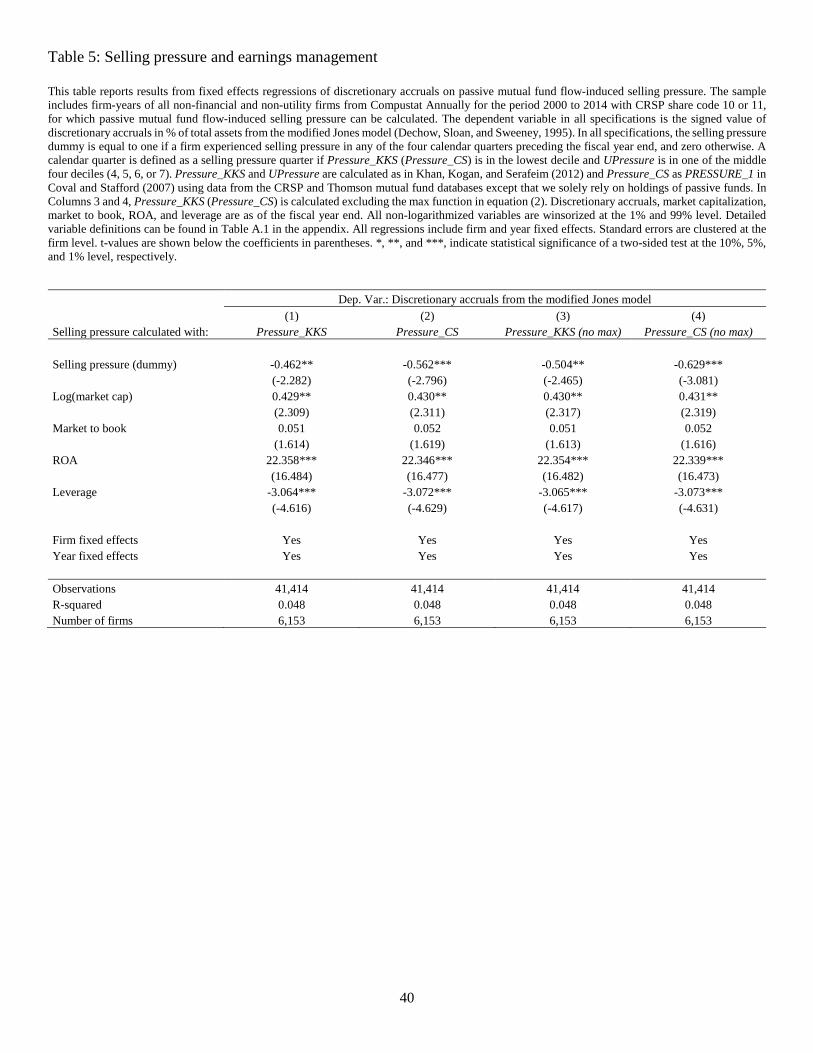
ified Jones model on our selling pressure dummy variables with results shown in Table 5. All

regressions include the full set of control variables and firm as well as year fixed effects. We borrow

the set of control variables from Fang, Huang, and Karpoff (2016). Standard errors are clustered

on the firm level. Column 1 reports results based on Pressure_KKS and Column 2 on Pressure_CS

as measures of mutual fund flow-induced selling pressure. The results in Column 1 show that if a

firm experienced selling pressure in any of the four quarters preceding the fiscal year end, discre-

tionary accruals are on average 0.46% lower at the fiscal year end. This accounts for a 37% (=

0.462/1.228) reduction in income-increasing earnings management compared to the unconditional

mean of discretionary accruals. Results in Column 2 are similar in terms of statistical and economic

significance.

The results in Columns 3 and 4 of Table 5 test for the concern that the continuous pressure

measures used to construct the selling pressure dummy, described in Section 2.1, might overesti-

mate mutual fund flow-induced selling pressure. This concern arises because the maximum func-

tion in equation (2) mechanically ensures that only positive changes in holdings are taken into

account for funds with large inflows, and only negative changes in holdings are taken into account

for funds with large outflows. By excluding the max function from the equation, we allow for

netting of the buying and selling of a single stock across funds with large flows in each quarter.

This makes selling pressure less likely to occur. As selling pressure becomes a comparatively rarer

event, the results in Columns 3 and 4 indeed suggest that managers respond more strongly to selling

pressure captured by these modified selling pressure measures. Overall, the coefficient estimates

21

on the mutual fund selling pressure variables in Table 5 suggest that financial markets have a dis-

ciplining effect on managers. Earnings management is significantly reduced in response to a re-

duction of the stock price identified by our measure of fund flow-induced selling pressure.

In the remainder of this sub-section, we conduct two robustness tests. First, we address the

concern that a small subsample of firms is driving our results. Most of the firms in our sample do

not experience selling pressure very often.7 Therefore, it is possible that the results from our base-

line regressions in Columns 1 and 2 of Table 5 are driven by a small fraction of firms that experi-

ence selling pressure frequently. To mitigate this concern, we rerun the regressions reported in

Columns 1 and 2 of Table 5 and exclude all firms that experience more than two quarters of selling

pressure during our sample period. This retains over 80% of firms in our sample, indicating that

for a majority of our firms fund-induced selling pressure is indeed a rare event. The results of

regressions run on this reduced sample are presented in Columns 1 and 2 of Table 6. The coeffi-

cients on the selling pressure indicator variable are larger than those obtained in our baseline re-

gressions in Table 5, indicating that firms respond more strongly if selling pressure is a compara-

tively rarer event. Furthermore, these findings reject the hypothesis that firms in the tail of the

selling pressure distribution drive our results. Rather, these findings support the idea that as selling

pressure becomes more salient, managers reduce earnings management even more.

Second, we test whether our results are robust to alternating the measures of earnings man-

agement. In Columns 3 and 4 of Table 6, we replace the discretionary accruals from the modified

Jones model with those from the Jones model in its original form. Given the mechanical relation

between the two models, we expect the results to be similar to those from Table 5. However, in

some instances the Jones model may understate earnings management (Dechow, Sloan and

7 For a distribution of the number of selling pressure quarters per firm see Table A.2 in the appendix.

22

Sweeney, 1995). Indeed, our results are slightly attenuated but still economically and statistically

significant when compared to the baseline regression.

In Columns 5 and 6 of Table 6, the dependent variable is the signed value of discretionary

accruals from the performance matched modified Jones model. The idea of this model is to control

for accounting performance in the estimation of discretionary accruals by subtracting the discre-

tionary accruals of the closest within-industry match in terms of ROA in each fiscal year. The

drawback of this approach is that it might reduce the power of the test (Dechow, Ge, and Schrand,

2010). Nevertheless, our results remain similar when compared to the baseline regression.

Finally, in Columns 7 and 8, we test for the robustness of our results using a different ap-

proach to estimating discretionary accruals. The unsigned discretionary accruals from the modified

Dechow-Dichev model are a function of past, present, and future cash flows. As such, this model

focuses on earnings management from short-term accruals and neglects long-term earnings man-

agement (Dechow, Ge, and Schrand, 2010). The significant coefficients on the selling pressure

dummy show that our previous results also hold when we calculate discretionary accruals using

this alternative model.

The question is to what extent our results uncover a causal effect of the reduction in share

prices on earnings management. In the end, the causality of the results in Tables 5 and 6 depends

on the ability of our measure of mutual fund flow-induced selling pressure to detect exogenous

shocks to the share price. We believe, however, that our results are difficult to reconcile with a

story based on reverse causality. Such a story would require that reductions in earnings manage-

ment lead a substantial number of funds to divest their holdings in the respective firm and trigger

outflows only at funds with holdings in firms that reduce earnings management. Given that we only

23

use passive mutual funds to estimate selling pressure, simultaneous and strategic selling of sub-

stantial amounts of shares of companies that recently reduced their earnings management seems to

be an unlikely explanation in the first place, even more so when these strategic divestures have to

lead to substantial outflows on the fund-level. In addition, all our models account for time and firm

fixed effects. These fixed effects help us to rule out alternative stories that could potentially explain

our results, for example that all or most firms suffer stock price drops at certain points in time

because investors withdraw substantial amounts from mutual funds in general. Moreover, our con-

struction of the selling pressure measure takes into account the general level of fund outflows at a

given point in time. The measure only classifies companies as being under price pressure if the

outflow at the funds invested into these companies is high compared to other companies in a given

quarter and if no other fund is stepping in to purchase the shares. It follows that we cannot fully

rule out alternative explanations, but we believe that our measure identifies plausibly exogenous

shocks to firms’ share prices. Therefore, our results help to establish a causal disciplining effect of

capital markets on corporate earnings management.

4. Peer Effects in Corporate Earnings Management

4.1 Identification of peer groups and descriptive statistics

To analyze whether firms manage their discretionary accruals in response to the earnings

management by peer firms, we first need to identify a firm’s peer group. To this end, we rely on

the text-based network industry classifications (TNIC) of Hoberg and Phillips (2016).8 These in-

8 These industry classifications can be downloaded at http://hobergphillips.usc.edu/. We are grateful to Gerard Hoberg and Gordon Phillips for making these data available.

24

dustry classifications use textual analysis to measure similarity of products mentioned in the prod-

uct descriptions provided by firms in their 10-K filings. TNIC classifications have a number of

desirable features, which make them superior to alternative industry classification schemes such as

the SIC, Fama French industries, or the North American Industry Classification System (NAICS)

to identify a firm’s peer group.9 Specifically, Hoberg and Phillips (2016) show that firms identified

as peers with TNIC are mentioned as actual peer firms by managers themselves. The TNIC also

allows for a continuous change of a peer group over time. Finally, in this classification, two firms

that are peers must not share an identical set of peers (i.e., this classification does not assume tran-

sitivity). Not surprisingly, recent papers on corporate peer effects also rely on TNIC to define peer

groups (Foucault and Fresard, 2014; Cao, Liang, Zhan, 2016).

To be included in our peer firm analysis, we require a firm to have at least three peers iden-

tified using TNIC in given year. We average all firm characteristics across a peer group and report

summary statistics of these averages in Panel A of Table 7. For the sake of completeness, we also

report firm characteristics for this (slightly) reduced sample in Panel B. On average, peer groups

are comprised of almost 59 firms (median: 31), and around 12% of firms in a peer group are subject

to mutual fund induced selling pressure in a given year. This proportion is very similar to the firm-

level occurrence of selling pressure. With regard to other company characteristics, peer firm aver-

ages are very similar to the average firm characteristics reported for our sample firms in Panel B.

Note that summary statistics of peer groups are calculated on values that are already averaged

across the peer group. Thus, percentiles and the standard deviation cannot be compared to firm-

level summary statistics. The firm characteristics in Panel B are very similar to those presented in

9 In robustness tests, we find that our peer effect results hold when using alternative industry classification schemes (3-digit SIC codes and FF48 industries).

25

Table 4. Hence, our requirement of at least three peer firms per firm-year does not seem to affect

sample characteristics.

4.2 Identifying peer effects in earnings management

As virtually all peer effects papers do, we face an identification challenge when estimating

peer effects. This challenge comes from a special type of endogeneity referred to as the “reflection

problem” (Manski, 1993; Leary and Roberts, 2014). The concern is that there might be a self-

selection of firms into peer groups. In the context of our study, shared unobservable characteristics

or preferences of peer group members might determine earnings management of all members of

the peer group, and thus lead to a correlation of earnings management within a peer group. To

overcome this identification problem, we need an exogenous event that affects earnings manage-

ment at one firm in the peer group, but does not directly affect earnings management at other firms

within the peer group. Arguably, our measure of passive mutual fund flow-induced selling pressure

represents such an exogenous shock. It triggers a reduction in discretionary accruals at the firm

experiencing fund flow-induced selling pressure, but is unlikely to directly affect discretionary

accruals at other firms in the peer group. Our measure of mutual fund flow-induced selling pressure

is caused by outflows at many different passive funds. As argued in Section 2.1, these flows are

plausibly exogenous to the affected firms and hence unlikely to be related to firm fundamentals,

even less so to peer firm fundamentals.

To examine whether firms adapt their earnings management following changes in earnings

management at peer firms, we exploit the disciplining effect of exogenous mutual fund flow-in-

duced selling pressure on peer firms’ earnings management. To this end, we regress a firm’s dis-

cretionary accruals in a given year on the fraction of peer firms that experience selling pressure.

26

We further control for average peer firm characteristics, for selling pressure at the sample firm, and

for the sample firm’s characteristics. We also include year and firm fixed effects. The results of

this regression, using Pressure_KKS and Pressure_CS as the respective measure of mutual fund

flow-induced selling pressure, are presented in Columns 1 and 2 of Table 8. The results in both

specifications suggest that a larger fraction of selling pressure at peer firms triggers a significant

reduction in discretionary accruals at our sample firms. These results are not only statistically, but

also economically significant. A one standard deviation increase in the fraction of peer firms ex-

periencing fund flow-induced selling pressure is associated with a decrease in discretionary accru-

als by 0.265 (0.283), or 23.309% (24.842%) of mean discretionary accruals.

A major concern with our analysis is that sample firms may experience fund flow-induced

selling pressure themselves and hence our identified reduction in discretionary accruals could ra-

ther be a first-order effect of a stock price shock, as identified in Section 3.2, rather than a peer

effect. To mitigate this concern, we control for the firms’ own stock price shocks in all regressions.

To further address this concern, we exclude all firms from our sample that experience at least one

selling pressure shock and retain only firms that never experience selling pressure during our sam-

ple period themselves. The drawback of this approach is that it substantially reduces sample size.

The results from estimating our baseline peer effect regressions in Columns 1 and 2 for this reduced

sample are reported in Columns 3 and 4 of Table 8. While the coefficients on the fraction of peer

firms that experience selling pressure remain similar in magnitude, the statistical significance is

reduced and the coefficient in Column 3 turns insignificant at conventional levels. The coefficient

in Column 4 is still significant at the 5% level. Overall, these findings confirm our previous find-

ings.

27

4.3 Actions vs. characteristics

Our results so far suggest that there are peer effects in corporate earnings management. Ac-

cording to Manski (1993) and Leary and Roberts (2014), there is a second aspect of the identifica-

tion challenge in identifying peer effects, namely the difficulty to determine the channels through

which peer effects operate. Specifically, it is unclear whether firms respond to the actions (i.e.,

changes in earnings management) or to the characteristics (e.g., profitability, size, or growth op-

portunities) of their peer firms. In a setting like ours, disentangling these two channels is challeng-

ing as the coefficient on the fraction of peers experiencing selling pressure in Table 8 captures both

effects (Leary and Roberts, 2014).

Hence, we follow a procedure similar to Leary and Roberts (2014) with the aim to disentangle

these two channels. We begin by noting that the coefficients on the peer firm control variables are

largely insignificant across the specifications in Table 8. This suggests that peer characteristics

only play a limited role in explaining earnings management at our sample firms. In a more sophis-

ticated test, we check under which circumstances firms adjust their earnings management. We are

especially interested whether a firm reduces earnings management if a large fraction of peers ex-

periences selling pressure but, on average, these peers do not reduce their earnings management.

To this end, we sort our sample firms into 25 two-way sorted buckets: First, we form quintiles

based on the fraction of peer firms that experience fund flow-induced selling pressure, conditional

on one firm in the peer group being shocked. Second, we form quintiles based on the average

change in discretionary accruals of peer firms. For each of the resulting 25 buckets, we present the

firm’s average change in discretionary accruals in Table 9.

Entries in each row show changes in discretionary accruals of a firm, holding fixed the frac-

tion of shocked peer firms, while varying the change in discretionary accruals of peer firms across

28

the five columns. For instance, the entry in Row 5 and Column 3 shows the change in discretionary

accruals for firms for which a large fraction of peer firms experiences selling pressure (Quintile 5),

and for which the change in discretionary accruals of these peer firms is in the middle quintile

(Quintile 3), and thus roughly zero. Indeed, changes in discretionary accruals of firms in this bucket

(-0.250) are statistically indistinguishable from zero. In fact, this is true for four out of the five

entries in Column 3. Further, a test for the difference in means between Rows 1 and 5 is insignifi-

cant across all columns. In contrast, we find a monotonic increase in the change in discretionary

accruals across columns (the only exception is Row 2) suggesting that our sample firms’ change in

discretionary accruals is closely linked to peer firms’ change in discretionary accruals. Consist-

ently, a test for the difference in means between Columns 1 and 5 is significant at the 1% level

across all five rows. Our interpretation of these results is as follows: Regardless of the fraction of

shocked peer firms, a firm only adjust its earnings management if peer firms also adjust earnings

management. If peer firms do adjust earnings management, firms adjust it in the same direction as

their peers. This suggests that firms especially respond to the actions of their peers. While we

acknowledge that these conclusions are based on results of univariate tests, we believe that they

add to our understanding of how peer effects in earnings management materialize.

4.4 Instrumental variables regressions

In an attempt to isolate the response of firms to the actions of their peers as opposed to their

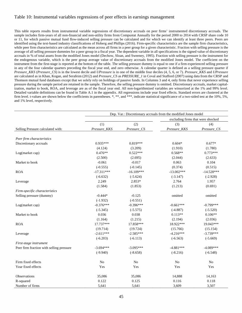
characteristics, and to determine the economic magnitude of this effect, we estimate instrumental

variables (IV) regressions. We instrument peer firms’ discretionary accruals with the fraction of

peer firms that experience selling pressure. To qualify as a valid instrument, the fraction of peer

firms that experience selling pressure has to satisfy both the exclusion restriction and the relevance

29

condition. The exclusion restriction requires that the fraction of a firm’s peers experiencing selling

pressure is not correlated with this firm’s discretionary accruals, except through its effect on the

endogenous variable, the average discretionary accruals of the peers. As discussed in Sections 2.1

and 3.2, our passive mutual fund selling pressure measure captures plausibly exogenous shocks

that are uncorrelated to firm characteristics. Thus, it seems unlikely that omitted peer firm charac-

teristics are correlated with a firm’s discretionary accruals as well as the exogenous peer firm

shocks. Further, as shown in Table 9, firms adjust discretionary accruals only if peer firms adjust

their discretionary accruals, but not in response to fund flow-induced price shocks at peer firms.

Finally, the coefficients on peer firm characteristics in Table 8 are largely insignificant. Jointly,

these findings lend strong support to the exclusion restriction of our instrument. The relevance

condition requires that the fraction of firms in a peer group experiencing mutual fund selling pres-

sure is significantly correlated with the average discretionary accruals of the peer group. This as-

sumption is testable and we report the coefficient estimates on our instrument from the first-stage

regression at the bottom of Table 10. Across all specifications, the coefficient on our instrument is

highly significant, with t-statistics between -6.5 and -9.9, confirming instrument relevance.

The results from the second-stage regressions are also reported in Table 10. Column 1 reports

the results from an IV regression in which the selling pressure variables are based on Pressure_KKS

and Column 2 reports the results based on Pressure_CS. In Columns 1 and 2, the coefficient on the

instrumented peer firm accruals measure is 0.94 and 0.82 with a t-statistic of 4.12 and 3.21, respec-

tively, confirming that firms decrease discretionary accruals in response to a decrease in discre-

tionary accruals at peer firms. A decrease in discretionary accruals of one standard deviation at

peer firms is associated with a decrease in discretionary accruals of 5.61% (4.92%) at sample firms.

In Columns 3 and 4, we drop all firms that experience selling pressure at any point during our

sample period to mitigate concerns of correlated selling pressure and a first-order selling pressure

30

effect at our sample firms. In this more restrictive sample, we obtain similar results, albeit both the

economic and statistical significance is somewhat reduced. In summary, the results in this section

further support the notion that capital markets are able to discipline managers. Moreover, capital

markets discipline managers not only via a direct channel, but also via an indirect channel, i.e.,

through spillover effects from peer firms that reduce earnings management.

5. Conclusion

In this paper, we analyze whether there are peer effects in corporate earnings management.

We overcome the identification problem common to nearly all peer effect papers by using fund

flow-induced selling pressure by passive mutual funds as an exogenous shock to stock prices (e.g.,

Coval and Stafford, 2007; Khan, Kogan, and Serafeim, 2012). We empirically confirm that such a

shock significantly affects firms’ stock returns. We then show that managers respond to such ex-

ogenous price shocks by reducing earnings management, suggesting a disciplining effect of stock

price pressure on managers. While fund flow-induced selling pressure triggers a reduction in dis-

cretionary accruals at the firm experiencing fund flow-induced selling pressure, it is unlikely to

directly affect discretionary accruals at other firms in the peer group.

To identify peer effects, we regress a firm’s discretionary accruals in a given year on the

fraction of peer firms that experience selling pressure, controlling for average peer firm character-

istics, selling pressure at the sample firm, sample firm characteristics, and year and firm fixed ef-

fects. We define peer groups based on the text-based network industry classifications (TNIC) of

Hoberg and Phillips (2016). The results of such regressions suggest that a larger fraction of peer

firms experiencing selling pressure is associated with a significant reduction in discretionary ac-

cruals at our sample firms. Specifically, we find a one standard deviation increase in the fraction

31

of peer firms experiencing fund flow-induced selling pressure to be associated with a decrease in

discretionary accruals by about 23% of mean discretionary accruals – an economically meaningful

effect. We alternatively estimate instrumental variables (IV) regressions in which we instrument

peer firms’ discretionary accruals with the fraction of peer firms that experience selling pressure

and find similar results.

32

References

Bizjak, J., M. Lemmon, and L. Naveen, 2008, Does the use of peer groups contribute to higher pay and less efficient compensation?, Journal of Financial Economics 90, 152-168.

Bizjak, J., M. Lemmon, and T. Nguyen, 2011, Are all CEOs above average? An empirical analysis of compensation peer groups and pay design, Journal of Financial Economics 100, 538-555.

Cao, J., H. Liang, and X. Zhan, 2016, Peer effects of corporate social responsibility, Working Pa-per, Chinese University of Hong Kong.

Chang, T., D. Solomon, and M. Westerfield, 2016, Looking for someone to blame: Delegation, cognitive dissonance, and the disposition effect, Journal of Finance 71, 267-302.

Cohen, L., and A. Frazzini, 2008, Economic links and predictable returns, Journal of Finance 63, 1977-2011.

Coval, J., and E. Stafford, 2007, Asset fire sales (and purchases) in equity markets, Journal of Financial Economics 86, 479-512.

Das, S., and H. Zhang, 2003, Rounding-up in reported EPS, behavioral thresholds, and earnings management, Journal of Accounting and Economics 35, 31-50.

DeAngelo, L., 1981, Auditor independence, ‘low balling’, and disclosure regulation, Journal of Accounting and Economics 3, 113-127.

Dechow, P., and I. Dichev, 2002, The quality of accruals and earnings: The role of accrual estima-tion errors, Accounting Review 77, 35-59.

Dechow, P., R. Sloan, and A. Sweeney, 1995, Detecting earnings management, Accounting Review 70, 193-225.

Dechow, P., W. Ge, and C. Schrand, 2010, Understanding earnings quality: A review of the prox-ies, their determinants and their consequences, Journal of Accounting and Economics 50, 344-401.

DeFond, M., and C. Park, 1997, Smoothing income in anticipation of future earnings, Journal of Accounting and Economics 23, 115-139.

Dyck, A., A. Morse, and L. Zingales, 2010, Who blows the whistle on corporate fraud?, Journal of Finance 65, 2213-2253.

Edmans, A., I. Goldstein, and W. Jiang, 2012, The real effects of financial markets: The impact of prices on takeovers, Journal of Finance 67, 933-971.

Fang, V., A. Huang, and J. Karpoff, 2016, Short selling and earnings management: A controlled experiment, Journal of Finance 71, 1251-1294.

Fishman, M., and K. Hagerty, 1992, Insider trading and the efficiency of stock prices, Rand Journal of Economics 23, 106-122.

Foucault, T., and L. Fresard, 2014, Learning from peers' stock prices and corporate investment, Journal of Financial Economics 111, 554-577.

33

Fracassi, C., 2016, Corporate finance policies and social networks, Management Science, forth-coming.

Georgarakos, D., M. Haliassos, and G. Pasini, 2014, Household debt and social interactions, Re-view of Financial Studies 27, 1404-1433.

Gleason, C., N. Jenkins, and W. Johnson, 2008, The contagion effects of accounting restatements, Accounting Review 83, 83-100.

Hameed, A., R. Morck, J. Shen, and B. Yeung, 2015, Information, analysts, and stock return comovement, Review of Financial Studies 28, 3153-3187.

Healy, P., and J. Wahlen, 1999, A review of the earnings management literature and its implications for standard setting, Accounting Horizons 13, 365-383.

Henning, L., D. Oesch, and M. Schmid, 2016, Stock underpricing and firm news disclosure, Work-ing Paper, University of St. Gallen.

Hoberg, G., G. Phillips, and N. Prabhala, 2014, Product market threats, payouts, and financial flex-ibility, Journal of Finance 69, 293-324.

Hoberg, G., and G. Phillips, 2016, Text-based network industries and endogenous product differ-entiation, Journal of Political Economy 124, 1423-1465.

Hsu, H.-C, A. Reed, and J. Rocholl, 2010, The new game in town: Competitive effects of IPOs, Journal of Finance 65, 495-528.

Hvide, H., and P. Östberg, 2015, Social interaction at work, Journal of Financial Economics 117, 628-652.

Irani, R., and D. Oesch, 2016, Analyst coverage and real earnings management: Quasi-experi-mental evidence, Journal of Financial and Quantitative Analysis 51, 589-627.

Jones, J., 1991, Earnings management during import relief investigations, Journal of Accounting Research 29, 193-228.

Kaustia, M., and S. Knüpfer, 2012, Peer performance and stock market entry, Journal of Financial Economics 104, 321-338.

Kaustia, M., and V. Rantala, 2015, Social learning and corporate peer effects, Journal of Financial Economics 117, 653-669.

Khan, M., L. Kogan, and G. Serafeim, 2012, Mutual fund trading pressure: Firm-level stock price impact and timing of SEOs, Journal of Finance 67, 1371-1395.

Kothari, S., A. Leone, and C. Wasley, 2005, Performance matched discretionary accrual measures, Journal of Accounting and Economics 39, 163-197.

Leary, M., and M. Roberts, 2014, Do peer firms affect corporate financial policy?, Journal of Fi-nance 69, 139-178.

34

Lee, G., and R. Masulis, 2009, Seasoned equity offerings: Quality of accounting information and expected flotation costs, Journal of Financial Economics 92, 443-469.

Leuz, C., D. Nanda, and P. Wysocki, 2003, Earnings management and investor protection: An international comparison, Journal of Financial Economics 69, 505-527.

Lou, D., 2012, A flow-based explanation for return predictability, Review of Financial Studies 25, 3457-3489.

Manski, C., 1993, Identification of endogenous social effects: The reflection problem, Review of Economic Studies 60, 531-542.

Massa, M., B. Zhang, and H. Zhang, 2015, The invisible hand of short selling: Does short selling discipline earnings management?, Review of Financial Studies 28, 1701-1736.

McNichols, M., 2004, Discussion of the quality of accruals and earnings: The role of accrual esti-mation errors, Accounting Review 77, 61-69.

Morsfield, S., and C. Tan, 2006, Do venture capitalists influence the decision to manage earnings in initial public offerings?, Accounting Review 81, 1119-1150.

Muslu, V., M. Rebello, and Y. Xu, 2014, Sell-side analyst research and stock comovement, Journal of Accounting Research 52, 911-954.

Nissim, D., and S. Penman, 2001, Ratio analysis and equity valuation: From research to practice, Review of Accounting Studies 6, 109-154.

Parsons, C.A., J. Sulaeman, and S. Titman, 2015, The geography of financial misconduct, Working Paper, University of California, San Diego.

Servaes, H., and A. Tamayo, 2014, How do industry peers respond to control threats?, Management Science 60, 380-399.

Shue, K., 2013, Executive networks and firm policies: Evidence from the random assignment of MBA peers, Review of Financial Studies 26, 1401-1442.

Watts, R., and J. Zimmerman, 1986, Positive accounting theory, Englewood Cliffs, NJ, Prentice-Hall.

35

Figure 1: Cumulative average abnormal return around pressure quarters This figure displays the quarterly cumulative average abnormal return in percent around selling pressure quarters. The sample includes firm-quarters of all non-financial and non-utility firms from Compustat Quarterly for the period 2000 to 2014 with CRSP share code 10 or 11, for which passive mutual fund flow-induced selling pressure can be calculated. For each firm-quarter observation, the abnormal return is calculated as a firm’s quarterly return minus the mean quarterly return of the universe of firms held by passive mutual funds in our sample in that quarter. Cumulative average abnormal returns are the running sum of the average abnormal returns starting in t-3. Selling pressure occurs in quarter t = 0. The time increments are in quarters. To ensure that t = 0 is the only quarter with selling pressure, the figure only displays the average abnormal return of firms that experience exactly one quarter of selling pressure. A calendar quarter is defined as a selling pressure quarter if Pressure_KKS is in the lowest decile and UPressure is in one of the middle four deciles (4, 5, 6 or 7). Pressure_KKS and UPressure are calculated as in Khan, Kogan, and Serafeim (2012) using data from the CRSP and Thomson mutual fund databases except that we solely rely on holdings of passive funds.

36

Table 1: Summary statistics of quarterly data This table reports selected summary statistics for the firm-quarter sample. The sample includes firm-quarters of all non-financial and non-utility firms from Compustat Quarterly for the period 2000 to 2014 with CRSP share code 10 or 11, for which passive mutual fund flow-induced selling pressure can be calculated. The three abnormal returns are market-adjusted quarterly abnormal returns. We adjust a firm’s quarterly return by subtracting either (1) the mean quarterly return of the universe of firms held by passive mutual funds in our sample, (2) the CRSP equally weighted return including distributions, or (3) the CRSP value weighted return including distributions. The selling pressure dummy is equal to one if a firm experiences selling pressure in a quarter, and zero otherwise. A calendar quarter is defined as a selling pressure quarter if Pressure_KKS (Pressure_CS) is in the lowest decile and UPressure is in one of the middle four deciles (4, 5, 6, or 7). Pressure_KKS and UPressure are calculated as in Khan, Kogan, and Serafeim (2012) and Pressure_CS as PRESSURE_1 in Coval and Stafford (2007) using data from the CRSP and Thomson mutual fund databases except that we solely rely on holdings of passive funds. Abnormal returns, market capitalization, market to book, ROA, and leverage are as of the end of the fiscal quarter. Selling pressure dummies are as of the end of the most recent calendar quarter. All non-logarithmized variables are winsorized at the 1% and 99% level. Detailed variable definitions can be found in Table A.1 in the appendix. Mean p25 p50 p75 Std. Dev. N Abnormal return (in %) Return - Sample mean return -0.265 -11.228 -1.103 9.074 19.516 150,362 Return - CRSP equally weighted return -0.083 -10.954 -0.804 9.210 19.579 150,362 Return - CRSP value weighted return 0.576 -10.173 -0.265 9.752 19.803 150,362 Selling pressure dummies Selling pressure (KKS) (dummy) 0.036 0.000 0.000 0.000 0.187 150,362 Selling pressure (CS) (dummy) 0.037 0.000 0.000 0.000 0.188 150,362 Controls Market cap ($millions) 3,002.051 126.655 447.286 1,627.619 8,901.427 150,362 Market to book 2.970 1.187 2.040 3.553 4.416 150,362 ROA 0.016 0.007 0.028 0.044 0.057 150,362 Leverage 0.285 0.007 0.218 0.449 0.305 150,362

37

Table 2: Univariate significance tests of average abnormal returns

This table reports the magnitude and significance of the average and median abnormal returns of the quarters displayed in Figure 1. The sample includes firm-quarters of all non-financial and non-utility firms from Compustat Quarterly for the period 2000 to 2014 with CRSP share code 10 or 11, for which passive mutual fund flow-induced selling pressure can be calculated. For each firm-quarter observation, the abnormal return is measured as a firm’s quarterly return minus the mean quarterly return of the universe of firms held by passive mutual funds in our sample in that quarter. Selling pressure occurs in quarter t = 0. The time increments are in quarters. To ensure that t = 0 is the only quarter with selling pressure, the table only displays the average abnormal return of firms that experience exactly one quarter of selling pressure. A calendar quarter is defined as a selling pressure quarter if Pressure_KKS is in the lowest decile and UPressure is in one of the middle four deciles (4, 5, 6 or 7). Pressure_KKS and UPressure are calculated as in Khan, Kogan, and Serafeim (2012) using data from the CRSP and Thomson mutual fund databases except that we solely rely on holdings of passive funds. Tests for differences in means are based on a simple t-test. Tests for differences in medians are based on a Wilcoxon signed-rank test. *, **, and ***, indicate statistical significance of a two-sided test at the 10%, 5%, and 1% level, respectively.

Quarter relative to selling pressure quarter Mean tests Median tests

Abnormal return t-value Abnormal return p-value -3 1.46 * 1.84 -0.98 0.91 -2 -0.50 -0.69 -1.34 0.14 -1 -0.02 -0.03 0.12 0.75 0 -4.55 *** -6.33 -3.11 *** 0.00 1 -1.35 * -1.83 -1.03 *** 0.01 2 -2.25 *** -3.15 -2.68 *** 0.00 3 0.50 0.66 -0.52 0.19

38

Table 3: First-stage regressions This table reports results from fixed effects regressions of the firms’ abnormal returns on quarterly selling pressure. The sample includes firm-quarters of all non-financial and non-utility firms from Compustat Quarterly for the period 2000 to 2014 with CRSP share code 10 or 11, for which passive mutual fund flow-induced selling pressure can be calculated. In all specifications, the dependent variable is the market-adjusted quarterly abnormal return. In Columns 1 and 2, the quarterly abnormal return is calculated as a firm’s quarterly return minus the mean quarterly return of the universe of firms held by passive mutual funds in our sample in that quarter. In Columns 3 and 4, the quarterly abnormal return is calculated as a firm’s quarterly return minus the CRSP equally weighted return including distributions. In Columns 5 and 6, the quarterly abnormal return is calculated as a firm’s quarterly return minus the CRSP value weighted return including distributions. In all specifications, the selling pressure dummy is equal to one if a firm experienced selling pressure in that quarter, and zero otherwise. A calendar quarter is defined as a selling pressure quarter if Pressure_KKS (Pressure_CS) is in the lowest decile and UPressure is in one of the middle four deciles (4, 5, 6, or 7). Pressure_KKS and UPressure are calculated as in Khan, Kogan, and Serafeim (2012) and Pressure_CS as PRESSURE_1 in Coval and Stafford (2007) using data from the CRSP and Thomson mutual fund databases except that we solely rely on holdings of passive funds. The selling pressure dummy is contemporaneous and all control variables are lagged by one quarter. Abnormal returns, market capitalization, market to book, ROA, and leverage are as of the end of the fiscal quarter. Selling pressure dummies are as of the end of the most recent calendar quarter. All non-logarithmized variables are winsorized at the 1% and 99% level. Detailed variable definitions can be found in Table A.1 in the appendix. All regressions include firm and year-quarter fixed effects. Standard errors are clustered at the firm level. t-values are shown below the coefficients in parentheses. *, **, and ***, indicate statistical significance of a two-sided test at the 10%, 5%, and 1% level, respectively.

Dep. Var.: Abnormal return (1) (2) (3) (4) (5) (6) Quarterly abnormal return esti-mated by subtracting: Sample mean CRSP EW CRSP VW Selling pressure calculated with: Pressure_KKS Pressure_CS Pressure_KKS Pressure_CS Pressure_KKS Pressure_CS Selling pressure (dummy) -1.272*** -1.060*** -1.271*** -1.060*** -1.267*** -1.066*** (-4.757) (-3.997) (-4.755) (-3.996) (-4.746) (-4.025) Log(market cap) -5.878*** -5.884*** -5.867*** -5.873*** -5.848*** -5.854*** (-65.425) (-65.510) (-65.328) (-65.412) (-65.171) (-65.255) Market to book 0.026* 0.026* 0.026* 0.026* 0.026* 0.026* (1.840) (1.843) (1.804) (1.807) (1.791) (1.794) ROA 52.477*** 52.461*** 52.496*** 52.480*** 52.690*** 52.674*** (30.586) (30.576) (30.608) (30.597) (30.749) (30.738) Leverage -1.930*** -1.936*** -1.937*** -1.943*** -1.896*** -1.902*** (-5.951) (-5.969) (-5.974) (-5.992) (-5.851) (-5.870) Lagged abnormal return 0.007** 0.007** 0.007*** 0.007*** 0.007** 0.007** (2.559) (2.563) (2.583) (2.587) (2.568) (2.572) Firm fixed effects Yes Yes Yes Yes Yes Yes Year-quarter fixed effects Yes Yes Yes Yes Yes Yes Observations 140,386 140,386 140,386 140,386 140,386 140,386 R-squared 0.038 0.038 0.043 0.043 0.067 0.067 Number of firms 5,890 5,890 5,890 5,890 5,890 5,890

39

Table 4: Summary statistics of annual dataset This table reports selected summary statistics for the firm-year sample. The sample includes firm-years of all non-financial and non-utility firms from Compustat Annually for the period 2000 to 2014 with CRSP share code 10 or 11, for which passive mutual fund flow-induced selling pressure can be calculated. Discretionary accruals in % of total assets are calculated from four different models: signed discretionary accruals from the modified Jones model (Dechow, Sloan, and Sweeney, 1995), signed discretionary accruals from the Jones (1991) model, signed discretionary accruals from the per-formance-matched modified Jones model (Kothari, Leone, and Wasley, 2005) and the absolute value of discretionary accruals from the modified Dechow-Dichev model augmented with firm fixed effects (Lee and Masulis, 2009). The selling pressure dummy is equal to one if a firm experienced selling pressure in any of the four calendar quarters preceding the fiscal year end, and zero otherwise. A calendar quarter is defined as a selling pressure quarter if Pressure_KKS (Pressure_CS) is in the lowest decile and UPressure is in one of the middle four deciles (4, 5, 6, or 7). Pressure_KKS and UPressure are calculated as in Khan, Kogan, and Serafeim (2012) and Pressure_CS as PRESSURE_1 in Coval and Stafford (2007) using data from the CRSP and Thomson mutual fund databases except that we solely rely on holdings of passive funds. Discretionary accruals, market capitalization, market to book, ROA, and leverage are as of the fiscal year end. All non-logarithmized variables are winsorized at the 1% and 99% level. Detailed variable definitions can be found in Table A.1 in the appendix.

Mean p25 p50 p75 Std. Dev. N Discretionary accruals (in % of total assets) Modified Jones 1.228 -5.342 0.837 7.897 16.409 41,414

Jones 1.315 -5.361 0.865 8.046 16.659 41,414

Performance matched mod. Jones -1.432 -10.982 -0.623 8.853 24.219 40,837

Modified Dechow-Dichev 4.752 1.489 3.239 6.147 4.999 37,830 Selling pressure dummies Selling pressure (KKS) (dummy) 0.121 0.000 0.000 0.000 0.326 41,414

Selling pressure (CS) (dummy) 0.122 0.000 0.000 0.000 0.328 41,414 Controls Market cap ($millions) 2,973.985 119.780 436.536 1,604.312 8,878.078 41,414

Market to book 2.918 1.158 2.017 3.543 4.360 41,414

ROA 0.054 0.030 0.106 0.164 0.220 41,414

Leverage 0.289 0.007 0.218 0.453 0.314 41,414

40

Table 5: Selling pressure and earnings management This table reports results from fixed effects regressions of discretionary accruals on passive mutual fund flow-induced selling pressure. The sample includes firm-years of all non-financial and non-utility firms from Compustat Annually for the period 2000 to 2014 with CRSP share code 10 or 11, for which passive mutual fund flow-induced selling pressure can be calculated. The dependent variable in all specifications is the signed value of discretionary accruals in % of total assets from the modified Jones model (Dechow, Sloan, and Sweeney, 1995). In all specifications, the selling pressure dummy is equal to one if a firm experienced selling pressure in any of the four calendar quarters preceding the fiscal year end, and zero otherwise. A calendar quarter is defined as a selling pressure quarter if Pressure_KKS (Pressure_CS) is in the lowest decile and UPressure is in one of the middle four deciles (4, 5, 6, or 7). Pressure_KKS and UPressure are calculated as in Khan, Kogan, and Serafeim (2012) and Pressure_CS as PRESSURE_1 in Coval and Stafford (2007) using data from the CRSP and Thomson mutual fund databases except that we solely rely on holdings of passive funds. In Columns 3 and 4, Pressure_KKS (Pressure_CS) is calculated excluding the max function in equation (2). Discretionary accruals, market capitalization, market to book, ROA, and leverage are as of the fiscal year end. All non-logarithmized variables are winsorized at the 1% and 99% level. Detailed variable definitions can be found in Table A.1 in the appendix. All regressions include firm and year fixed effects. Standard errors are clustered at the firm level. t-values are shown below the coefficients in parentheses. *, **, and ***, indicate statistical significance of a two-sided test at the 10%, 5%, and 1% level, respectively. Dep. Var.: Discretionary accruals from the modified Jones model (1) (2) (3) (4) Selling pressure calculated with: Pressure_KKS Pressure_CS Pressure_KKS (no max) Pressure_CS (no max) Selling pressure (dummy) -0.462** -0.562*** -0.504** -0.629*** (-2.282) (-2.796) (-2.465) (-3.081) Log(market cap) 0.429** 0.430** 0.430** 0.431** (2.309) (2.311) (2.317) (2.319) Market to book 0.051 0.052 0.051 0.052 (1.614) (1.619) (1.613) (1.616) ROA 22.358*** 22.346*** 22.354*** 22.339*** (16.484) (16.477) (16.482) (16.473) Leverage -3.064*** -3.072*** -3.065*** -3.073*** (-4.616) (-4.629) (-4.617) (-4.631) Firm fixed effects Yes Yes Yes Yes Year fixed effects Yes Yes Yes Yes Observations 41,414 41,414 41,414 41,414 R-squared 0.048 0.048 0.048 0.048 Number of firms 6,153 6,153 6,153 6,153

41

Table 6: Selling pressure and earnings management – Robustness tests This table reports results from fixed effects regressions of alternative measures of discretionary accruals on passive mutual fund flow-induced selling pressure. The sample includes firm-years of all non-financial and non-utility firms from Compustat Annually for the period 2000 to 2014 with CRSP share code 10 or 11, for which passive mutual fund flow-induced selling pressure can be calculated. In Columns 1 and 2, the dependent variable is the signed value of discretionary accruals in % of total assets from the modified Jones model (Dechow, Sloan, and Sweeney, 1995), in Columns 3 and 4 it is the signed value of discretionary accruals in % of total assets from the Jones (1991) model, in Columns 5 and 6 it is the signed value of discretionary accruals in % of total assets from the performance-matched modified Jones model (Kothari, Leone, and Wasley, 2005), and in Columns 7 and 8 it is the absolute value of discretionary accruals in % of total assets from the modified Dechow-Dichev model augmented with firm fixed effects (Lee and Masulis, 2009). In Columns 1 and 2, firms that experience more than two quarters of selling pressure during the sample period are excluded. In all specifications, the selling pressure dummy is equal to one if a firm experienced selling pressure in any of the four calendar quarters preceding the fiscal year end, and zero otherwise. A calendar quarter is defined as a selling pressure quarter if Pressure_KKS (Pressure_CS) is in the lowest decile and UPressure is in one of the middle four deciles (4, 5, 6, or 7). Pressure_KKS and UPressure are calculated as in Khan, Kogan, and Serafeim (2012) and Pressure_CS as PRESSURE_1 in Coval and Stafford (2007) using data from the CRSP and Thomson mutual fund databases except that we solely rely on holdings of passive funds. Discretionary accruals, market capitalization, market to book, ROA, and leverage are as of the fiscal year end. All non-logarithmized variables are winsorized at the 1% and 99% level. Detailed variable definitions can be found in Table A.1 in the appendix. All regressions include firm and year fixed effects. Standard errors are clustered at the firm level. t-values are shown below the coefficients in parentheses. *, **, and ***, indicate statistical significance of a two-sided test at the 10%, 5%, and 1% level, respectively.

Dep. Var.: Discretionary accruals max 2 quarters pressure (1) (2) (3) (4) (5) (6) (7) (8) Discretionary accruals from: Mod. Jones model Jones model Matched mod. Jones model Mod. Dechow-Dichev model Selling pressure (dummy) calculated with: Pressure_KKS Pressure_CS Pressure_KKS Pressure_CS Pressure_KKS Pressure_CS Pressure_KKS Pressure_CS Selling pressure (dummy) -0.774** -0.862*** -0.438** -0.543*** -0.683** -0.955*** -0.139** -0.198*** (-2.397) (-2.785) (-2.125) (-2.640) (-2.026) (-2.863) (-2.181) (-3.207) Log(market cap) 0.444** 0.488** 0.498*** 0.499*** 0.159 0.162 -0.291*** -0.290*** (2.085) (2.337) (2.656) (2.659) (0.593) (0.604) (-5.379) (-5.367) Market to book 0.076* 0.043 0.057* 0.057* -0.019 -0.019 0.058*** 0.058*** (1.912) (1.128) (1.759) (1.764) (-0.368) (-0.365) (5.567) (5.570) ROA 21.966*** 22.358*** 22.255*** 22.244*** 7.384*** 7.361*** -2.063*** -2.068*** (14.841) (15.433) (16.125) (16.118) (3.680) (3.668) (-4.992) (-5.005) Leverage -3.970*** -3.589*** -3.018*** -3.025*** -3.031*** -3.045*** 0.639*** 0.636*** (-4.968) (-4.629) (-4.490) (-4.502) (-3.205) (-3.221) (2.917) (2.905) Firm fixed effects Yes Yes Yes Yes Yes Yes Yes Yes Year fixed effects Yes Yes Yes Yes Yes Yes Yes Yes Observations 31,493 31,956 41,414 41,414 40,837 40,837 37,830 37,830 R-squared 0.051 0.051 0.048 0.048 0.003 0.003 0.018 0.019 Number of firms 5,429 5,463 6,153 6,153 6,123 6,123 5,516 5,516

42

Table 7: Summary statistics of the peer firm sample

This table reports selected summary statistics for the firm-year sample for which we can identify at least three peers. The sample includes firm-years of all non-financial and non-utility firms from Compustat Annually for the period 2000 to 2014 with CRSP share code 10 or 11, for which passive mutual fund flow-induced selling pressure can be calculated. Peers are identified using the text-based industry classifications of Hoberg and Phillips (2016). Firm-specific characteristics are the sample firm characteristics, while peer firm averages are calculated as the mean across all firms in a peer group for a given characteristic. Fraction with selling pressure is the average of all selling pressure dummies for a peer group in a fiscal year. Signed discretionary accruals are in % of total assets from the modified Jones model (Dechow, Sloan, and Sweeney, 1995). The selling pressure dummy is equal to one if a firm experienced selling pressure in any of the four calendar quarters preceding the fiscal year end, and zero otherwise. A calendar quarter is defined as a selling pressure quarter if Pressure_KKS (Pressure_CS) is in the lowest decile and UPressure is in one of the middle four deciles (4, 5, 6, or 7). Pressure_KKS and UPressure are calculated as in Khan, Kogan, and Serafeim (2012) and Pressure_CS as PRESSURE_1 in Coval and Stafford (2007) using data from the CRSP and Thomson mutual fund databases except that we solely rely on holdings of passive funds. Discretionary accruals, market capitalization, market to book, ROA, and leverage are as of the fiscal year end. All non-logarithmized variables are winsorized at the 1% and 99% level. Detailed variable definitions can be found in Table A.1 in the appendix. Mean p25 p50 p75 Std. Dev. N Panel A: Peer firm averages Number of peers 58.642 12.000 31.000 78.000 67.218 35,086 Modified Jones (in % of total assets) 0.673 -2.589 0.325 3.487 6.003 35,086 Fraction with selling pressure (KKS) 0.122 0.030 0.111 0.179 0.107 35,086 Fraction with selling pressure (CS) 0.120 0.029 0.103 0.176 0.110 35,086 Market cap ($millions) 3,249.185 1,415.179 2,486.454 4,109.134 2,894.692 35,086 Market to book 2.973 1.976 2.723 3.784 1.477 35,086 ROA 0.046 0.013 0.093 0.139 0.138 35,086 Leverage 0.273 0.159 0.243 0.367 0.147 35,086 Panel B: Firm-specific characteristics Modified Jones (in % of total assets) 1.138 -5.291 0.865 7.848 16.319 35,086 Selling pressure (KKS) (dummy) 0.116 0.000 0.000 0.000 0.321 35,086 Selling pressure (CS) (dummy) 0.116 0.000 0.000 0.000 0.321 35,086 Market cap ($millions) 2,982.858 128.497 448.278 1,610.498 8,854.722 35,086 Market to book 2.888 1.167 2.020 3.502 4.248 35,086 ROA 0.052 0.028 0.106 0.164 0.223 35,086 Leverage 0.282 0.005 0.208 0.443 0.311 35,086

43

Table 8: Peer effects in earnings management

This table reports results on peer effects in earnings management from fixed effects regressions of firms’ discretionary accruals in a given year on the fraction of peer firms that experience selling pressure, controlling for average peer firm characteristics, selling pressure at the sample firms, and the sample firms characteristics. The sample includes firm-years of all non-financial and non-utility firms from Compustat Annually for the period 2000 to 2014 with CRSP share code 10 or 11, for which passive mutual fund flow-induced selling pressure can be calculated and for which we can identify at least three peers. Peers are identified using the text-based industry classifications of Hoberg and Phillips (2016). Firm-specific characteristics are the sample firm characteristics, while peer firm characteristics are calculated as the mean across all firms in a peer group for a given characteristic. Fraction with selling pressure is the average of all selling pressure dummies for a peer group in a fiscal year. The dependent variable in all specifications is the signed value of discretionary accruals in % of total assets from the modified Jones model (Dechow, Sloan, and Sweeney, 1995). Fraction with selling pressure is the average of all individual firms’ selling pressure dummies calculated over a firm’s peer group in a fiscal year. The selling pressure dummy is equal to one if a firm experienced selling pressure in any of the four calendar quarters preceding the fiscal year end, and zero otherwise. A calendar quarter is defined as a selling pressure quarter if Pressure_KKS (Pressure_CS) is in the lowest decile and UPressure is in one of the middle four deciles (4, 5, 6, or 7). Pressure_KKS and UPressure are calculated as in Khan, Kogan, and Serafeim (2012) and Pressure_CS as PRESSURE_1 in Coval and Stafford (2007) using data from the CRSP and Thomson mutual fund databases except that we solely rely on holdings of passive funds. In Columns 3 and 4, only firms that never experience selling pressure during the sample period are retained in the sample. Therefore, the selling pressure dummy is omitted. Discretionary accruals, market capitalization, market to book, ROA, and leverage are as of the fiscal year end. All non-logarithmized variables are winsorized at the 1% and 99% level. Detailed variable definitions can be found in Table A.1 in the appendix. All regressions include firm and year fixed effects. Standard errors are clustered at the firm level. t-values are shown below the coefficients in parentheses. *, **, and ***, indicate statistical significance of a two-sided test at the 10%, 5%, and 1% level, respectively. Dep. Var.: Discretionary accruals from the modified Jones model excluding firms that were shocked (1) (2) (3) (4) Selling pressure calculated with: Pressure_KKS Pressure_CS Pressure_KKS Pressure_CS Peer firm characteristics Fraction with selling pressure -2.479*** -2.570*** -2.428 -4.055** (-2.977) (-3.207) (-1.499) (-2.410) Log(market cap) 0.303 0.303 0.446 0.444 (1.487) (1.489) (1.255) (1.156) Market to book 0.175* 0.177* 0.106 0.262 (1.870) (1.894) (0.680) (1.536) ROA 3.703* 3.661* 2.651 3.862 (1.667) (1.649) (0.740) (1.016) Leverage 1.471 1.457 -2.249 -2.398 (1.173) (1.161) (-0.997) (-0.969) Firm-specific characteristics Selling pressure (dummy) -0.361 -0.400* omitted omitted (-1.624) (-1.793) Log(market cap) 0.436** 0.435** 0.356 0.299 (2.066) (2.061) (1.072) (0.840) Market to book 0.059 0.058 0.137** 0.163** (1.597) (1.590) (2.022) (2.435) ROA 22.548*** 22.549*** 21.778*** 22.514*** (15.183) (15.187) (9.802) (9.786) Leverage -2.794*** -2.797*** -4.466*** -4.157*** (-3.768) (-3.772) (-3.342) (-3.043) Firm fixed effects Yes Yes Yes Yes Year fixed effects Yes Yes Yes Yes Observations 35,086 35,086 14,888 14,163 R-squared 0.052 0.053 0.057 0.060 Number of firms 5,641 5,641 3,609 3,507

44

Table 9: Disentangling actions and characteristics in peer effects

This table reports the change in discretionary accruals, from fiscal year t-1 to t, for 25 different buckets of firms. Buckets are formed along two dimensions: (1) quintiles of the fraction of peer firms experiencing a shock, given that one peer firm is shocked are shown vertically, and (2) quintiles of the average change in discretionary accruals of peer firms are shown horizontally. The entries display the average change in discretionary accruals for firms placed in the respective bucket. Signed discretionary accruals are in % of total assets from the modified Jones model (Dechow, Sloan, and Sweeney, 1995). The sample includes firm-years of all non-financial and non-utility firms from Compustat Annually for the period 2000 to 2014 with CRSP share code 10 or 11, for which passive mutual fund flow-induced selling pressure can be calculated and for which we can identify at least three peers. Peers are identified using the text-based industry classifications of Hoberg and Phillips (2016). Further, results of tests for differences in means between columns 5 and 1 and rows 5 and 1 are displayed. t-values are shown in parentheses. *, **, and ***, indicate statistical significance of a two-sided test at the 10%, 5%, and 1% level, respectively. Peer Firm Average Discretionary Accruals Change - Quintiles Fraction of Peer Firms Shocked - Quintiles 1 2 3 4 5 5 - 1 1 -7.482 *** -1.022 0.581 0.771 7.167 *** 14.649 *** (-8.232) (-1.504) (0.985) (1.119) (8.59) 2 -7.636 *** -2.581 *** 1.718 *** 0.963 4.885 *** 12.521 *** (-8.971) (-4.357) (2.987) (1.571) (6.472) 3 -7.375 *** -2.317 *** -0.036 2.504 *** 5.922 *** 13.296 *** (-11.623) (-4.123) (-0.065) (4.69) (8.483) 4 -7.657 *** -1.873 *** -0.680 2.021 *** 6.302 *** 13.958 *** (-10.357) (-3.214) (-1.096) (3.384) (9.327) 5 -6.274 *** -1.051 * -0.250 0.750 5.766 *** 12.040 *** (-8.074) (-1.693) (-0.452) (1.286) (9.24) 5 - 1 1.208 -0.029 -0.831 -0.021 -1.400

45

Table 10: Instrumental variables regressions of peer effects in earnings management

This table reports results from instrumental variable regressions of discretionary accruals on peer firms’ instrumented discretionary accruals. The sample includes firm-years of all non-financial and non-utility firms from Compustat Annually for the period 2000 to 2014 with CRSP share code 10 or 11, for which passive mutual fund flow-induced selling pressure can be calculated and for which we can identify at least three peers. Peers are identified using the text-based industry classifications of Hoberg and Phillips (2016). Firm-specific characteristics are the sample firm characteristics, while peer firm characteristics are calculated as the mean across all firms in a peer group for a given characteristic. Fraction with selling pressure is the average of all selling pressure dummies for a peer group in a fiscal year. The dependent variable in all specifications is the signed value of discretionary accruals in % of total assets from the modified Jones model (Dechow, Sloan, and Sweeney, 1995). Fraction with selling pressure is the instrument for the endogenous variable, which is the peer group average value of discretionary accruals from the modified Jones model. The coefficient on the instrument from the first-stage is reported at the bottom of the table. The selling pressure dummy is equal to one if a firm experienced selling pressure in any of the four calendar quarters preceding the fiscal year end, and zero otherwise. A calendar quarter is defined as a selling pressure quarter if Pressure_KKS (Pressure_CS) is in the lowest decile and UPressure is in one of the middle four deciles (4, 5, 6, or 7). Pressure_KKS and UPressure are calculated as in Khan, Kogan, and Serafeim (2012) and Pressure_CS as PRESSURE_1 in Coval and Stafford (2007) using data from the CRSP and Thomson mutual fund databases except that we solely rely on holdings of passive funds. In Columns 3 and 4, only firms that never experience selling pressure during the sample period are retained in the sample. Therefore, the selling pressure dummy is omitted. Discretionary accruals, market capital-ization, market to book, ROA, and leverage are as of the fiscal year end. All non-logarithmized variables are winsorized at the 1% and 99% level. Detailed variable definitions can be found in Table A.1 in the appendix. All regressions include year fixed effects. Standard errors are clustered at the firm level. t-values are shown below the coefficients in parentheses. *, **, and ***, indicate statistical significance of a two-sided test at the 10%, 5%, and 1% level, respectively. Dep. Var.: Discretionary accruals from the modified Jones model excluding firms that were shocked (1) (2) (3) (4) Selling Pressure calculated with: Pressure_KKS Pressure_CS Pressure_KKS Pressure_CS Peer firm characteristics Discretionary accruals 0.935*** 0.819*** 0.604* 0.677* (4.124) (3.209) (1.910) (1.780) Log(market cap) 0.476** 0.522*** 0.568** 0.773*** (2.500) (2.695) (2.044) (2.633) Market to book -0.061 -0.017 0.063 0.104 (-0.555) (-0.145) (0.374) (0.515) ROA -17.311*** -16.109*** -13.002*** -14.528*** (-6.632) (-5.624) (-3.147) (-2.928) Leverage 2.249 2.853* 2.764 1.957 (1.584) (1.853) (1.213) (0.691) Firm-specific characteristics Selling pressure (dummy) -0.444* -0.125 omitted omitted (-1.932) (-0.551) Log(market cap) -0.376*** -0.396*** -0.661*** -0.799*** (-5.345) (-5.575) (-4.887) (-5.520) Market to book 0.036 0.038 0.113** 0.106** (1.164) (1.215) (2.194) (2.036) ROA 17.737*** 17.858*** 18.922*** 19.043*** (19.714) (19.724) (15.766) (15.154) Leverage -2.611*** -2.585*** -4.216*** -3.739*** (-6.203) (-6.113) (-6.563) (-5.669) First-stage instrument Peer firm fraction with selling pressure -3.694*** -3.095*** -4.881*** -4.089*** (-9.940) (-8.658) (-8.216) (-6.548) Firm fixed effects No No No No Year fixed effects Yes Yes Yes Yes Observations 35,086 35,086 14,888 14,163 R-squared 0.122 0.125 0.116 0.118 Number of firms 5,641 5,641 3,609 3,507

46

Appendix

Figure A.1.: Distribution of selling pressure quarters during the sample period

This figure displays the distribution of selling pressure over the sample period. The sample includes firm-quarters of all non-financial and non-utility firms from Compustat Quarterly for the period 2000 to 2014 with CRSP share code 10 or 11, for which passive mutual fund flow-induced selling pressure can be calculated. Time increments are in calendar quarters. In each calendar quarter, the density of firms that experience selling pressure is displayed. A calendar quarter is defined as a selling pressure quarter if Pressure_KKS is in the lowest decile and UPressure is in one of the middle four deciles (4, 5, 6 or 7). Pressure_KKS and UPressure are calculated as in Khan, Kogan, and Serafeim (2012) using data from the CRSP and Thomson mutual fund databases except that we solely rely on holdings of passive funds. The red vertical lines indicate the fourth calendar quarter of each year.

47

Table A.1: Variable definitions

Variable Definition Discretionary accruals Modified Jones Signed value of discretionary accruals from the modified Jones model (Dechow et al. (1995)), constructed as in Irani

and Oesch (2016). Discretionary accruals are the difference between a firm's actual accruals and its predicted accruals from the modified Jones model. The model is run for each fiscal year and Fama-French 48 industry separately. A minimum of 20 observations per fiscal year-industry regression is required for years t through t-4. This variable is in % of total assets.

Jones Signed value of discretionary accruals from the Jones (1991) model, constructed similar to Irani and Oesch (2016). Discretionary accruals are the difference between a firm's actual accruals and its predicted accruals from the Jones (1991) model. The model is run for each fiscal year and Fama-French 48 industry separately. A minimum of 20 observations per fiscal year-industry regression is required for years t through t-4. This variable is in % of total assets.

Performance-matched modified Jones Performance-matched discretionary accruals as in Kothari et al. (2005), constructed as in Fang et al. (2016). Discre-tionary accruals are the difference between a firm's actual accruals and its predicted accruals from the modified Jones model. The model is run for each fiscal year and Fama-French 48 industry separately. A minimum of 20 observations per fiscal year-industry regression is required for years t through t-4. Performance-matched discretionary accruals are the difference between a firm's discretionary accruals and the discretionary accruals of the closest match in terms of ROA (see below) in the same fiscal year and Fama-French 48 industry. This variable is in % of total assets.

Modified Dechow-Dichev Absolute value of discretionary accruals from the modified Dechow Dichev (2002) model augmented with firm fixed effects, constructed as in Lee and Masulis (2009). Discretionary accruals are the difference between a firm's actual accruals and its predicted accruals from the modified Dechow Dichev (2002) model augmented with firm fixed effects in the estimation of accruals. The fixed effects model is run only once over the entire panel. This variable is in % of total assets.

Selling pressure dummies Selling pressure_KKS quarterly (dummy) A dummy variable that equals one if there is selling pressure in the calendar quarter, and zero otherwise. A calendar

quarter is defined as a selling pressure quarter if Pressure_KKS is in the lowest decile and UPressure is in one of the middle four deciles (4, 5, 6 or 7). Deciles are calculated for every quarter separately. Pressure_KKS and UPressure are constructed as in Khan, Kogan, and Serafeim (2012). Only the holdings of passive funds are used to construct this measure.

Selling pressure_CS quarterly (dummy) This dummy is defined analogously to Selling pressure_KKS quarterly using Pressure_CS, which is constructed as PRESSURE_1 in Coval and Stafford (2007).

48

Selling pressure_KKS (dummy) A dummy variable that equals one if there was selling pressure in any of the four calendar quarters preceding the

fiscal year end, and zero otherwise. A calendar quarter is defined as a selling pressure quarter if Pressure_KKS is in the lowest decile and UPressure is in one of the middle four deciles (4, 5, 6 or 7). Deciles are calculated for every quarter separately. Pressure_KKS and UPressure are constructed as in Khan, Kogan, and Serafeim (2012). Only the holdings of passive funds are used to construct this measure.

Selling pressure_CS (dummy) This dummy is defined analogously to Selling pressure_KKS using Pressure_CS, which is constructed as PRES-SURE_1 in Coval and Stafford (2007).

Selling pressure_KKS (no max) (dummy) This dummy is defined analogously to Selling pressure_KKS. The max function is excluded in the construction of Pressure_KKS.

Selling pressure_CS (no max) (dummy) This dummy is defined analogously to Selling pressure_CS. The max function is excluded in the construction of Pressure_CS.

Control variables Log(market cap) quarterly Natural logarithm of the market value of equity. The market value of equity is calculated with data from CRSP, by

multiplying the closing price with the number of shares outstanding on the last trading day of the fiscal quarter. Log(market cap) quarterly = ln(1000*shrout*abs(prc)).

Market to book quarterly Market value of equity divided by the book value of equity at the end of the fiscal quarter. The market value of equity is calculated with data from CRSP, by multiplying the closing price with the number of shares outstanding on the last trading day of the fiscal quarter. Market value of equity in $ = abs(prc)*shrout*1,000. Book value of equity is from Compustat, as of the end of the fiscal quarter. Book value of equity in $ = ceqq*1,000,000.

ROA quarterly Operating income before depreciation of the fiscal quarter scaled by the book value of assets at the end of the fiscal quarter. ROA quarterly = oibdpq/atq.

Leverage quarterly Leverage as of the end of the fiscal quarter, calculated as in Fang et al. (2016). Long-term debt plus debt in current liabilities is divided by the sum of long-term debt, debt in current liabilities, and total shareholder's equity.

Leverage quarterly = (dlttq + dlcq)/(dlttq + dlcq + seqq).

Log(market cap) Natural logarithm of the market value of equity. Market value of equity is calculated with data from CRSP, by mul-tiplying the closing price with the number of shares outstanding on the last trading day of the fiscal year. Log(market cap) = ln(1000*shrout*abs(prc))

49

Market to book Market value of equity divided by the book value of equity. Market value of equity is calculated with data from CRSP, by multiplying the closing price with the number of shares outstanding on the last trading day of the fiscal year. Market value of equity in $ = abs(prc)*shrout*1,000. Book value of equity is from Compustat, as of the fiscal year end. Book value of equity in $ = ceq*1,000,000

ROA Operating income before depreciation scaled by the book value of assets at the fiscal year end. ROA = oibdp/at

Leverage Leverage as of the fiscal year end, calculated as in Fang et al. (2016). Long-term debt plus debt in current liabilities is divided by the sum of long-term debt, debt in current liabilities, and total shareholder's equity. Leverage = (dltt + dlc)/(dltt + dlc + seq)

Abnormal returns

Return - Sample mean return Abnormal quarterly return in % measured as the firm's quarterly return minus the mean quarterly return of all firms in the sample. Return data is from CRSP.

Return - CRSP equally weighted return Abnormal quarterly return in % measured as the firm's quarterly return minus the CRSP equally weighted return including distributions. Return data is from CRSP.

Return - CRSP value weighted return Abnormal quarterly return in % measured as the firm's quarterly return minus the CRSP value weighted return in-cluding distributions. Return data is from CRSP.

50

Table A.2: Frequency distribution of selling pressure quarters per firm This table reports the number of selling pressure quarters each distinct firm experiences during our sample period. The sample includes firm-quarters of all non-financial and non-utility firms from Compustat Quarterly for the period 2000 to 2014 with CRSP share code 10 or 11, for which passive mutual fund flow-induced selling pressure can be calculated. A calendar quarter is defined as a selling pressure quarter if Pressure_KKS is in the lowest decile and UPressure is in one of the middle four deciles (4, 5, 6, or 7). Pressure_KKS and UPressure are calculated as in Khan, Kogan, and Serafeim (2012) using data from the CRSP and Thomson mutual fund databases except that we solely rely on holdings of passive funds.

Number of quarters with selling pressure per firm N % Cumulative % 0 3,742 60.82 60.82 1 1,026 16.67 77.49 2 527 8.56 86.06 3 346 5.62 91.68 4 200 3.25 94.93 5 124 2.02 96.94 6 87 1.41 98.36 7 51 0.83 99.19 8 30 0.49 99.67 9 9 0.15 99.82 10 8 0.13 99.95 11 1 0.02 99.97 12 2 0.03 100.00 Sum 6,153 100.00 -