Pentzer Et Al-2014-Journal of Field Robotics

Model-based Prediction of Skid-steer Robot KinematicsUsing Online Estimation of Track Instantaneous Centersof Rotation

• • • • • • • • • • • • • • • • • • • • • • • • • • • • • • • • • • • •

Jesse Pentzer and Sean BrennanDepartment of Mechanical and Nuclear Engineering, The Pennsylvania State University, University Park, Pennsylvania 16802e-mail: [email protected], [email protected] ReichardApplied Research Lab, The Pennsylvania State University, University Park, Pennsylvania 16802e-mail: [email protected]

Received 31 January 2014; accepted 4 February 2014

This paper presents a kinematic extended Kalman filter (EKF) designed to estimate the location of track instan-taneous centers of rotation (ICRs) and aid in model-based motion prediction of skid-steer robots. Utilizing anICR-based kinematic model has resulted in impressive odometry estimates for skid-steer movement in previousworks, but estimation of ICR locations was performed offline on recorded data. The EKF presented here utilizesa kinematic model of skid-steer motion based on ICR locations. The ICR locations are learned by the filterthrough the inclusion of position and heading measurements. A background on ICR kinematics is presented,followed by the development of the ICR EKF. Simulation results are presented to aid in the analysis of noiseand bias susceptibility. The experimental platforms and sensors are described, followed by the results of filterimplementation. Extensive field testing was conducted on two skid-steer robots, one with tracks and anotherwith wheels. ICR odometry using learned ICR locations predicts robot position with a mean error of −0.42 mover 40.5 m of travel during one tracked vehicle test. A test consisting of driving both vehicles approximately1,000 m shows clustering of ICR estimates for the duration of the run, suggesting that ICR locations do not varysignificantly when a vehicle is operated with low dynamics. C© 2014 Wiley Periodicals, Inc.

1. INTRODUCTION

Skid-steering is a commonly utilized locomotion mecha-nism for mobile robots and large industrial and agriculturalvehicles. A skid-steer system has no steering mechanismand instead changes vehicle direction by adjusting the speedof the left and right side wheels or tracks. The simplicity, ro-bustness, and zero-radius turn capability of skid-steeringmake it an excellent choice for all-terrain and teleoperatedvehicles, but the complex track/terrain interaction devel-oped during a skid-steer maneuver is difficult to model.Hence, when compared to steered or two-wheel robots, it isquite difficult to predict the future position of a skid-steerrobot.

The number of unmanned ground vehicles utilized bycivilian and military organizations has increased signifi-cantly in the past decade, the vast majority of which uti-lize skid-steer mobility. Most unmanned ground systemscurrently fielded are teleoperated and have limited or noautonomous functions, and one of the largest obstacles to

Direct correspondence to Sean Brennan, e-mail: [email protected]

increased autonomy is improved navigation of unmannedground vehicles for the safety of soldiers and civilians inthe operational area (Robotic Systems Joint Project Office,2012).

Improving navigation in unmanned vehicles reliesheavily on understanding the complex track/terrain inter-actions of skid-steer vehicles due to significant slippageduring movement. The research presented by Anousakishowed that a differential drive, two-wheel vehicle modelcannot be used to accurately represent a skid-steer ve-hicle due to track and wheel slippage (Anousaki andKyriakopoulos, 2004). Much work has been completed inthe terramechanics and vehicle dynamics fields developingcomplete models of skid-steer vehicle motion (Wong, 2008;Wong and Chiang, 2001). However, these models are com-plex, require extensive knowledge of terrain properties, andare often focused on vehicles much larger than most mobilerobots.

The past decade has seen increased interest in model-ing with a focus on mobile robots. The bulk of this researchcan be divided into two areas, the first being those robotsthat utilize a dynamic model of the vehicle with inertia and

Journal of Field Robotics 31(3), 455–476 (2014) C© 2014 Wiley Periodicals, Inc.View this article online at wileyonlinelibrary.com • DOI: 10.1002/rob.21509

ABNER CHAVEZ

Highlight

456 • Journal of Field Robotics—2014

tire stiffness or track mechanical properties (Chuy, Collins,Yu, & Ordonez, 2009; Ferretti and Girelli, 1999; Le, Rye, &Durrant-Whyte, 1997; Ward and Iagnemma, 2008; Wong andChiang, 2001; Yi, Song, Zhang, & Goodwin, 2007a; Zweiri,Seneviratne, & Althoefer, 2003). This area of research is oftencentered on how the forces acting between the terrain andthe locomotion system are modeled. Slip is inherently in-cluded in such models through the tractive force, whichis generally modeled as a function of tire or track slip-page. The second branch of research has focused on utiliz-ing kinematic models of vehicle movement to estimate slip(Kozlowski and Pazderski, 2004; Martınez, Mandow,Morales, Pedraza, & Garcıa-Cerezo, 2005; Moosavianand Kalantari, 2008; Morales, Martınez, Mandow, Garcıa-Cerezo, & Pedraza, 2009; Wang and Low, 2008; Yi, Zhang,Song, & Jayasuriya, 2007b; Yi et al., 2009). Measurementsfrom wheel encoders, inertial measurement units (IMUs),and position systems such as GPS and cameras are usedto estimate slip by comparing movement inputs with mea-sured motion. Most recently, vision-based algorithms havebeen utilized to detect slip by comparing inputs with mea-sured motion using stereo or monocular vision odome-try algorithms (Angelova, Matthies, Helmick, & Perona,2006; Milella, Reina, & Siegwart, 2006; Nister, Naroditsky,& Bergen, 2004; Song, Seneviratne, & Althoefer, 2011a,2011b). Rather than using vision information to estimatemodel parameters, there has also been significant work inutilizing visual information directly for motion estimationand mapping (Botterill, Mills, & Green, 2011; Lambert,Furgale, Barfoot, & Enright, 2012; Marks, Howard,Bajracharya, Cottrell, & Matthies, 2009). Range sensors,specifically LIDAR systems, have also been used for motionestimation in the absence of direct position measurementssuch as GPS (Almeida and Santos, 2013).

This paper presents research utilizing a kinematicmodel to predict vehicle motion by learning track instan-taneous centers of rotation (ICRs) relative to the groundusing an extended Kalman filter (EKF). There are manyother examples in the literature that also utilize kinematicmodels. In Yi et al. (2009), an EKF is used to integrate mea-surements from an IMU and fuse them with virtual velocitymeasurements created using wheel encoder measurementsand estimates of slip generated from a kinematic model ofmotion. Experimental results show position estimate errorsbelow 25 cm for approximately 40 m of travel on a complexpath. It is interesting to note that bounds are enforced oncalculated slips to ensure EKF convergence, which is similarto a modification of the ICR kinematic model needed in thiswork. An EKF is also used by Dar to estimate track slip andvehicle slip angle using measurements of vehicle positionand heading (Dar and Longoria, 2010). Further work in uti-lizing Kalman filters for slip estimation has been presentedin Rogers-Marcovitz, George, Seegmiller, & Kelly (2012),where a delayed-state EKF is utilized for slip estimation, and

in Vinh Ha, Ha, & Lee (2013), where a Kalman filter formu-lated to estimate slip runs in parallel with a navigation EKFalgorithm. The algorithm performs well on recorded data,but was not implemented on the vehicle. Burke presenteda least-squares method of estimating slip implemented inconjunction with a kinematic model (Burke, 2012). The esti-mator is guaranteed to converge, but simulation results donot generally show convergence when slip values are con-stantly changing. No implementation is presented. Moosa-vian presented a method of estimating slippage by fittingexponential functions of turn radius to experimental data(Moosavian and Kalantari, 2008). The slip models are uti-lized to control a skid-steer vehicle along a path with goodresults. Research presented in Martınez et al. (2005) utilizesthe same kinematic model presented in this paper, but ICRlocations are learned offline using a genetic algorithm op-erating on recorded data. Error values are not provided,but figures show impressive odometry over approximately30 m of travel.

The research presented here is different in that the pre-viously mentioned works relied on analysis of recorded datato calculate certain track/terrain interaction parameters orestimated slip coefficients rather than ICR locations. In thiswork, an EKF is used to learn ICR locations during operationusing track speed, heading, and position measurements.Learned ICR locations are then used to estimate movementof the vehicle when external position measurements areabsent. ICR locations are modeled as constant values dis-turbed by random noise. The constant value assumptionstems from previous work where ICR locations are shownto remain within small bounded regions for robots operat-ing at low speeds on hard, flat terrain (Martınez et al., 2005).Thus, the low speed and hard, flat terrain assumptions ap-ply to the work presented here as well. Experimental resultsshow convergence of ICR estimates within 5–15 s of driving,depending on the movement of the vehicle.

The ICR locations estimated by the EKF provide a map-ping from vehicle wheel or track speeds to vehicle forwardand angular velocity. This enables more accurate odome-try when external position systems fail or become inaccu-rate; one example of this is when GPS signals are blocked,or when there are multipath GPS signals. This use of theICR EKF as a GPS backup is explored through extensivefield-testing in this work. Other possible applications of es-timated ICR locations include modeling power usage inskid-steer wheeled and tracked vehicles, controlling skid-steer vehicles by calculating needed track or wheel speedfrom desired vehicle movement, and in the detection of pureslip and vehicle immobilization.

The remaining sections are organized as follows.Section 2 gives an introduction to ICR kinematics, andSection 3 describes the EKF developed to estimate ICR loca-tion. Section 4 provides details on the skid-steer robots usedduring testing. The simulation used during evaluation of the

Journal of Field Robotics DOI 10.1002/rob

Pentzer et al.: Model-based Prediction of Skid-steer Robot Kinematics • 457

Figure 1. Diagram of ICR locations on the skid-steer robot.

algorithm is described in Section 5, and details of field-testing are provided in Section 6. Finally, a discussion of theresults and conclusions are given in Section 7.

2. APPROXIMATING THE KINEMATICS OFSKID-STEER ROBOTS

The dynamics of skid-steer vehicles are complex due to thelarge amounts of track slippage and terrain deformation thatoccur during movement. Dynamic Models of skid-steer dy-namics have been developed and verified, but the modelscontain numerous parameters, most involving terrain prop-erties that must be identified, often through experimentalanalysis. It has been shown that the movement of skid-steervehicles can be estimated accurately using knowledge oftrack ICR locations (Martınez et al., 2005).

Figure 1 shows the track ICR locations relative to aright-hand body-fixed coordinate system (X, Y, Z). The ICRlocation between the robot chassis and the ground, yICRv

, is

yICRv= vx

ωz

, (1)

where vx is the vehicle velocity along the X axis and ωz is theangular velocity of the vehicle. The ICR locations betweenthe tracks and the ground can be found by introducing theindividual track velocities, yielding

yICRl= −V l

x − vx

ωz

, (2)

yICRr= −V r

x − vx

ωz

, (3)

where yICRland yICRr

are the ICR locations for the left- andright-hand tracks, respectively, V l

x is the velocity of the left-hand track relative to the body of the robot, and V r

x is the

velocity of the right-hand track relative to the body of therobot. The X coordinate of the vehicle ICR location, xICRv

, isfound using

xICRv= − vy

ωz

, (4)

where vy is the lateral velocity of the vehicle. The X locationof the left track ICR can be calculated in a similar way to Eq.(2) using

xICRl= V l

y − vy

ωz

. (5)

Because the spinning of the track is assumed to induce novelocity to the track in the Y direction, V l

y = 0 and Eq. (5)reduces to

xICRl= − vy

ωz

. (6)

A similar analysis can be conducted for xICRrwith the result

xICRr= xICRl

= xICRv= − vy

ωz

. (7)

Thus, the three ICR locations, those of the vehicle, left track,and right track, lie along a straight line parallel to the body-fixed Y axis.

It should be noted that the values of yICRvrange within

±∞ depending on vehicle motion. However, the values ofyICRr

, yICRl, and xICRv

remain bounded. As vehicle motionapproaches that of driving in a straight line, the numeratorsand denominators of Eqs. (2)–(4) are infinitesimals of thesame order, resulting in finite values for the ICR locations(Martınez et al., 2005).

Equations (2)–(4) can be solved to express body framevelocities in terms of input track velocities and track ICRlocations. The resulting kinematic model,



vx = V rx yICRl

− V lxyICRr

yICRl− yICRr

, (8)

vy = (V lx − V r

x )xICRv

yICRl− yICRr

, (9)

wz = − V lx − V r

x

yICRl− yICRr

, (10)

forms the basis for the EKF described in the next section.The denominator of Eqs. (8)–(10) consists of yICRl

− yICRr, so

the possibility of division by zero must be addressed. Dueto slippage, the ICR locations must lie outside the trackcenterlines (Martınez et al., 2005). Thus, to have divisionby zero, the tracks or wheels would need to lie along thesame line, a physical impossibility for a skid-steer mobilerobot. It is also interesting to note that values of yICRl

and yICRr

approach infinity when the robot is stationary but the tracksare spinning. This may occur when the vehicle operates on alow friction surface or becomes stuck in some way. Rapidlyincreasing values of yICRl

and yICRrcould be used to detect

occurrences of pure slip such as these.

3. EKF FOR ICR ESTIMATION

This section will discuss the formulation of a kinematic EKFfor the estimation of the ICR locations. Starting with thekinematic equations (8)–(10), the velocities of the robot inthe north, N , and east, E, directions are found to be

N = vx cos ψ − vy sin ψ, (11)

E = vx sin ψ + vy cos ψ, (12)

where ψ is the heading angle as defined in Figure 2. Theequations of motion for the robot are

⎡⎢⎢⎢⎢⎢⎢⎣

N

E

ωz

yICRr

yICRl

xICRv

⎤⎥⎥⎥⎥⎥⎥⎦

=

⎡⎢⎢⎢⎢⎢⎢⎢⎣

vx cos ψ − vy sin ψ + wN

vx sin ψ + vy cos ψ + wE

− V lx−V r

x

yICRl−yICRr

+ wω

wr

wl

wx

⎤⎥⎥⎥⎥⎥⎥⎥⎦

, (13)

where wN -wx are additive zero-mean Gaussian processnoises. Previous work in ICR kinematics has shown thatthe ICR locations remain within a small bounded region forrobots traveling at low speeds on hard, flat terrain (Martınezet al., 2005). These criteria apply to the majority of testingin this work, so the ICR locations are modeled as constantsdisturbed by random noise, and results presented later con-firm that ICR locations remain bounded to the same regionregardless of maneuver type. Additional testing to explorethe variation of ICR locations with increasing speed is pre-sented in Section 6.6. The kinematic model is discretizedusing the Euler method, with the result

Figure 2. Relation between body frame and fixed framethrough heading angle ψ .

⎡⎢⎢⎢⎢⎢⎢⎣

Nk

Ek

ψk

yICRrk

yICRlk

xICRvk

⎤⎥⎥⎥⎥⎥⎥⎦

=

⎡⎢⎢⎢⎢⎢⎢⎣

Nk−1 + �tVNk−1 + �twN

Ek−1 + �tVEk−1 + �twE

ψk−1 + �tωzk−1 + �twω

yICRrk−1 + �twr

yICRlk−1 + �twl

xICRvk−1 + �twx

⎤⎥⎥⎥⎥⎥⎥⎦

, (14)

where �t is the time step.The EKF utilizes the discrete time model Eq. (14), de-

noted compactly as

x−k = f(x+

k−1, uk−1, 0), (15)

where x−k is the propagated state at the current time step,

x+k−1 is the propagated and updated state from the previ-

ous time step, uk−1 is the vector of control inputs consist-ing of left and right track velocity, and the third entry inf(x+

k−1, uk−1, 0) denotes setting the process noise to zero forpropagation. Throughout this paper, a superscript “−” de-notes a value propagated but not updated with measure-ments, and a superscript “+” denotes a value propagatedand updated with measurements.

The state covariance, P, is propagated using

P−k = Fk−1P+

k−1FTk−1 + Lk−1Qk−1LT

k−1, (16)

where Fk−1 and Lk−1 are Jacobian matrices defined as

Fk−1 = ∂fk−1

∂x

∣∣∣∣x+k−1

, (17)

Lk−1 = ∂fk−1

∂w

∣∣∣∣x+k−1

= �tI6×6, (18)



and Q is the process noise covariance, assumed to be uncor-related.

To update the state estimate, measurements of vehiclenorth and east positions, NGPS and EGPS, and vehicle head-ing, ψV , are available from sensors on the robot and collectedin the vector y as

yk =⎧⎨⎩

NGPS

EGPS

ψV

⎫⎬⎭

k

. (19)

These direct measurements of states result in the measure-ment equations

hk =⎧⎨⎩

N + vN

E + vE

ψ + vψ

⎫⎬⎭

k

, (20)

where vN -vψ represent additive measurement noise. Thefilter gain is calculated using

Kk = P−k HT

k (HkP−k HT

k + MkRkMTk )−1, (21)

where Hk and Mk are Jacobian matrices defined as

Hk = ∂hk

∂x

∣∣∣∣x−k

=⎡⎣ 1 0 0 0 0 0

0 1 0 0 0 00 0 1 0 0 0

⎤⎦ (22)

Mk = ∂hk

∂v

∣∣∣∣x+k

= I3×3. (23)

Finally, the state and covariance estimates are updated using

x+k = x−

k + Kk[yk − hk(x−k , 0)], (24)

P+k = (I6×6 − KkHk)P−

k . (25)

3.1. Investigation of Conditions for ICRIdentification

The structure of the kinematic model and measurementmodel provide insight into the ability of the presentedEKF to estimate ICR locations. The state update Eq. (24)computes the correction to the state through the productof the Kalman gain, Kk , and the measurement innova-tion, yk − hk(x−

k , 0). The measurement innovation consistsonly of the difference between the measured and estimatednorth position, east position, and the heading of the vehicle,and therefore the coupling between measurement innova-tion and the ICR location update comes about through theKalman gain.

It is most interesting to determine when the EKF willnot update the ICR location estimates. This occurs when thebottom three rows of the Kalman gain are zero, the conditionfor which can be found from Eq. (21). The term P−

k HTk in

Eq. (21) is evaluated to be

P−k HT

k =

⎡⎢⎢⎢⎢⎢⎢⎢⎢⎢⎣

σ 2N σNσE σNσψ

σNσE σ 2E σEσψ

σNσψ σEσψ σ 2ψ

σNσyICRrσEσyICRr

σψσyICRr

σNσyICRlσEσyICRl

σψσyICRl

σNσxICRvσEσxICRv

σψσxICRv

⎤⎥⎥⎥⎥⎥⎥⎥⎥⎥⎦

, (26)

where σ is the variance of the estimator error for the sub-scripted state at the current time step. The final three rowsof the Kalman gain will become zero when the covariancesbetween the estimate errors of robot pose and ICR locationsare zero. The state error covariance matrix P is initialized tobe a diagonal matrix, and the process noise is assumed to beadditive and uncorrelated, leaving the term Fk−1P+

k−1FTk−1 in

Eq. (16) as the only contribution to the estimate error covari-ance between robot pose and ICR location. The linearizedkinematic model matrix, Fk−1, can be split into four parts as

Fk−1 =[

FK3×3 FI3×3

03×3 I3×3

], (27)

where FK3×3 and FI3×3 are the Jacobians of the first three rowsof Eq. (14) with respect to the estimated robot pose and ICRlocations, respectively. When the state error covariance P isa diagonal matrix, such as when it is initialized, the onlynonzero terms in the calculation of covariance between es-timate errors of robot pose and ICR locations, computed byEq. (16), consist of terms in FI3×3 multiplied by ICR loca-tion estimate error variances. Therefore, estimation of ICRlocations depends on the values of FI3×3 being nonzero.

Two examples of the terms in FI3×3 are

∂Nk

∂yICRr

= �t

((VryICRl

− VlyICRr) cos ψ

(yICRl− yICRr

)2

− Vl cos ψ

yICRl− yICRr

− (Vl − Vr )xICRvsin ψ

(yICRl− yICRr

)2

)(28)

and

∂Nk

∂xICRv

= −�t(Vl − Vr ) sin ψ

yICRl− yICRr

. (29)

When the track or wheel speeds are equal, Vr = Vl , Eqs. (28)and (29) evaluate to zero, as do all other terms in FI3×3 . Thefinal conclusion of this analysis is that the EKF estimatesof ICR locations are updated only when the vehicle is turn-ing, or Vr �= Vl . Thus, the ICR EKF conditionally updates theestimates of ICR location based on vehicle motion. This isnot thought to be a large weakness of the ICR EKF becauseground mobile robots do not generally spend significant pe-riods of time driving in straight lines. Many current groundmobile robot designs feature cameras fixed to the chassis ofthe vehicle, forcing the vehicle to turn to view other areasof the operational environment. The filter structures alsoprevents adjustment of the ICR location estimates when thevehicle is stationary, which is beneficial in that previously



Figure 3. Skid-steer robots used during experimental testing.

learned ICR information is retained when the vehicle mo-mentarily stops moving.

4. TESTING PLATFORMS

The two skid-steer robots shown in Figure 3 were used for alltesting in this research. The tracked vehicle on the left wasdesigned and built at The Pennsylvania State University,and the wheeled vehicle on the right is the RMP400 fromSegway Robotics. The same real-time kinematic (RTK) GPSand attitude heading reference system (AHRS) were utilizedon each robot. Final drive shaft speeds on the tracked robotwere measured using optical encoders. Encoders were un-necessary on the RMP 400 because the integrated motor con-trollers report measured wheel speeds at 100 Hz. High-levelcomputation and data recording are done on an embeddedcomputer running the open-source robot-operating-system(ROS) architecture (Quigley et al., 2009).

The optical encoders on the tracked robot produce2,048 pulses per resolution, and the interface chip providesquadrature encoding, producing a change of 8,192 countsfor one revolution, or 0.0439 degrees per count. The encodercount update rate is approximately 100 Hz. The Xsens MTi-G AHRS provides roll, pitch, and yaw data at 100 Hz withdynamic accuracy of 1 degree root mean square (rms) and aresolution of 0.05 degrees. The Hemisphere A325 Smart An-tenna RTK GPS system communicates with a base stationthrough a radio serial modem and provides position and ve-locity updates at 20 Hz with an accuracy of 0.01 m rms. Onthe tracked vehicle, the embedded computer communicatescommanded rpm values for each track to a commercial dcmotor controller at 10 Hz. The encoder signals are madeavailable to the motor controller, which regulates trackspeed using proportional-integral-derivative (PID) control.The integrated motor controllers on the RMP 400 accept

inputs of desired linear and angular vehicle velocity andperform closed-loop control on wheel speeds to achieve thedesired inputs.

The mass of the tracked robot is 37 kg, and the distancebetween the centers of the left and right tracks is 0.52 m.The contact area of each track is approximately 461.3 cm2.The width of the wheeled robot is 0.61 m, and it is muchheavier with a mass of 118 kg. The weight distribution of thetracked vehicle is symmetrical laterally, but the motors anddrive batteries are placed toward the front of the vehicle,moving the center of mass approximately 10 cm forwardfrom the vehicle frame center. The weight distribution of thewheeled robot is very symmetrical, resulting in a center ofmass at the geometric center of the vehicle’s contact square.

The ICR EKF was implemented on each vehicle suchthat propagation occurs at 100 Hz and measurements ofheading from the AHRS and position from the GPS areutilized whenever available. All data streams in the systemare logged within the ROS architecture into binary files thatare available for later analysis and playback.

5. SIMULATION AND ANALYSIS OF ICR EKF

The ICR EKF was developed and tested using MATLAB toinvestigate convergence properties and resilience to noise.The true state model consisted of the kinematic equations inEqs. (8)–(10). ICR locations of yICRr

= 0.5 m, yICRl= −0.75 m,

and xICRv= −0.25 m were chosen based on the test robot di-

mensions of 0.51 m in width by 0.72 m in length. Measure-ments of position and heading were created by corruptingoutputs of the kinematic model with zero-mean randomGaussian noise of standard deviation 0.01 m for positionand 1 degree for heading. These error values were chosento simulate the performance of the sensors used in testing,described in Section 4.



The process noise covariance and measurement noisecovariance must be defined to run the EKF. The processnoise covariance Q was set to be

Q =

⎡⎢⎢⎢⎢⎢⎢⎣

0.22 0 0 0 0 00 0.22 0 0 0 00 0 ( 5π

180 )2 0 0 00 0 0 0.012 0 00 0 0 0 0.012 00 0 0 0 0 0.012

⎤⎥⎥⎥⎥⎥⎥⎦

. (30)

The first two diagonal terms of Q represent the processnoise of 0.1 m/s standard deviation in the north and east.To determine noise level, the tracked robot was driven ina straight line by commanding a track velocity of 0.40 m/sto each side, which is a speed representative of the experi-mental data presented in the following sections. The stan-dard deviation of the noise in the velocity output of theRTK GPS system was calculated and used as the processnoise in the north and east. The heading measurement ofthe AHRS system was processed for the same straight linerun to determine the process noise on the vehicle heading,which is the third diagonal term. The remaining three di-agonal terms relate to the ICR estimates and were chosenby manually adjusting the process noise to minimize errorsbetween simulated and measured positions of the vehicle,using offline recordings of one data run. While more formalminimization methods could have been used, the sensitiv-ity of the estimation process to these parameters was lowenough that errors in manual tuning clearly do not affectthe feasibility of the algorithm, and they only affect conver-gence rates slightly.

The measurement noise covariance matrix R was set as

R =⎡⎣ 0.012 0 0

0 0.012 00 0 ( 1π

180 )2

⎤⎦ , (31)

where the values of 0.01 m in the position measurementvariances represent the accuracy of the GPS system, and thevalue of ( 1π

180 ) radians represents the accuracy of the AHRSsystem, both described in Section 4.

A comparison of the EKF position estimate and trueposition is given in Figure 4. The accurate position andheading measurements enable the filter to match the truepath while quickly learning the correct ICR locations ofyICRr

= 0.5, yICRl= −0.75, and xICRv

= −0.25, as shown inFigure 5. Some modifications to the kinematic equationswere necessary to avoid divergence of the filter estimate inthe presence of noise and disturbances. The next phase ofsimulation focused on this area.

5.1. Preventing Divergence Due to ICR SignInversion

It was found in initial testing that filter estimates of ICR lo-cations diverged during a significant number of simulation

−2 0 2 4 6 8 10 12−10

−8

−6

−4

−2

0

2

East (m)

Nor

th (

m)

START

END

TrueEKF

Figure 4. Simulated position and EKF estimate for the trackedrobot.

0 2 4 6 8 10−3

−2

−1

0

1

2

3

Time (s)

ICR

Est

imat

e (m

)

y

ICRr

yICRl

xICRv

Figure 5. EKF estimated ICR positions during simulation forthe tracked robot.

runs. The simulation was repeated with initial ICR loca-tion estimates ranging from 2 to −2. The results, shown inFigure 6, indicate that yICRr

converges only when the initialcondition is greater than zero. A similar plot for yICRl

showsconvergence only when yICRl

is initialized with a negativenumber.

The kinematic modeling equations, given in Eqs. (4)–(10), were modified to ensure filter convergence. With re-spect to the defined body frame, shown in Figure 1, the leftICR location will always be negative and the right ICR lo-cation will always be positive. To enforce this knowledge ofICR location, the kinematics were modified to be



0 20 40 60 80 100−30

−25

−20

−15

−10

−5

0

5

Time (s)

y ICR

r (m

)

Figure 6. Plot of yICRrestimate during tracked vehicle simu-

lations for initial conditions ranging from 2 through −2 usingkinematic equations (8)–(10).

vx = V rx yICRl

− V lxyICRr

− ∣∣yICRl− yICRr

∣∣ , (32)

vy =(V l

x − V rx

)xICRv


∣∣ , (33)

wz = − V lx − V r

x


∣∣ (34)

such that the difference value yICRl− yICRr

will always havethe correct negative sign. With this change, the filter con-verges regardless of initial condition or variation after ini-tialization. The result is that for any initial condition, theICR location converges to the correct value as shown inFigure 7.

5.2. Filter Convergence Response to Changing ICRLocations and Vehicle Turn Radius

The system model used in the ICR EKF, given in Eq. (14),assumes the ICR locations are constant values disturbedby random noise. It is important to investigate how thisassumption affects the ability of the ICR EKF to estimatechanging ICR locations, which may occur when a robotdrives from one terrain to another. This scenario was exam-ined in simulation, with the results shown in Figure 8. Thetimes at which the ICR locations changed are also labeled inFigure 8. The convergence time for the filter after a changein ICR location ranged from 100 to 140 s. In this work, thedefinition of rise time (Kuo and Golnaraghi, 2003) is used todefine the convergence rate, e.g., the time from 10% changein ICR estimate to when the estimate is within 90% of thefinal value. The time of convergence in Figure 8 is slow,

0 20 40 60 80 100−2

−1

0

1

2

3

Time (s)

y ICR

r (m

)

Figure 7. Plot of yICRrestimate during tracked vehicle simu-

lations for initial conditions ranging from 2 through −2 withmodified kinematic equations (32)–(34).

Figure 8. Simulation run with changing ICR locations. Timesof ICR changes are labeled with vertical lines at 175 and 350 s.

but it can be improved significantly by inflating the ICRestimate state error covariances when a change in terrain isdetected. This process was also simulated and is shown inFigure 9. The convergence times are much faster and rangefrom 0.03 to 0.17 s when the state error covariance is in-flated to 100 m2 at the time the true ICR locations change.Detection of terrain changes using camera and LIDAR out-puts is an expected area of future work for this research.This will enable the inflation of state error covariances andfaster convergence times even when a constant ICR modelis utilized.

The change in convergence rate with vehicle turn ra-dius was also investigated in simulation. The results, shown



Figure 9. Simulation run with changing ICR locations and in-flation of ICR location estimate error covariance at ICR change.Times of ICR changes are labeled with vertical lines at 175 and350 s.

0 0.5 1 1.5 20

0.5

1

1.5

2

Radius of Turn (m)

Tim

e of

Con

verg

ence

Aft

er I

CR

Cha

nge

(s)

Figure 10. Average convergence time of ICR estimates fromEKF as a function of increasing turn radius over 20 simulationruns. There is a clear increase in convergence time as the turnradius increases.

in Figure 10, show a clear increase in convergence time withlarger turn radii. The convergence times given in Figure 10are the averages over 20 simulation runs at the correspond-ing turn radius. The correlation between turn radius andconvergence time is expected because of the relation be-tween vehicle angular rate and the ability of the ICR EKF toidentify ICR locations, as discussed in Section 3.1.

0 20 40 60 80 100−0.1

0

0.1

0.2

0.3

0.4

0.5

0.6

Time (s)

Tra

ck V

eloc

ity (

m/s

)

Encoder

Motor Controller

Figure 11. Comparison of commanded and measured lefttrack velocity for the tracked vehicle.

5.3. Response of Filter Due to Input Bias and Noise

The preceding simulation results contain realistic sensornoise on the position and heading measurements, but noisewas not introduced on the input track velocities. Twosources of left and right track velocities are available onthe robots used for testing: commanded velocity to the mo-tor controller and measured track velocity from encodersor wheel velocity from motor controllers. A comparison ofthe two values for a representative run with the trackedrobot is shown in Figure 11. There is a disadvantage to us-ing either signal as an input to the filter. The commandedspeed given to the motor controller is noise-free, but a biasexists between the commanded speed and the measuredspeed of the track. The track speed calculated from encodermeasurements is more accurate, but is corrupted by noisefrom differentiating encoder counts. Understanding howthe ICR EKF responds to biased or noisy inputs is key forimplementation on a robot.

Some insight into the effect of noise and bias on ICR es-timates can be gained by analyzing the ICR kinematic equa-tions given in Eqs. (8)–(10). To simplify analysis, it is helpfulto assume symmetric ICR locations such that yICRr

= −yICRl.

Making this substitution in the ICR kinematic equationsyields

vx = V rx + V l

x

2, (35)

vy =(V l

x − V rx

)xICRv

2yICRl

, (36)

wz = −V lx − V r

x

2yICRl

. (37)



0 0.1 0.2 0.3 0.4 0.5−1

−0.5

0

0.5

1

Standard Deviation of Input Noise (m/s)

Err

or in

IC

R E

stim

ate

(m)

y

ICRr

yICRl

xICRv

Figure 12. Error in ICR location estimate as a function of in-creasing input noise on the simulated tracked robot.

Starting with the expression for longitudinal velocity, vx ,the addition of the input track speeds V r

x and V lx makes lon-

gitudinal velocity fairly impervious to random noise butsusceptible to biases. The magnitude of track velocity dur-ing operation is around 0.1–0.5 m/s, as shown in Figure 11.The longitudinal velocity will have the correct sign untilnoise values reach unreasonable magnitudes. Bias terms,however, are additive in longitudinal velocity and will biasICR location estimates. Bias and noise have an opposite ef-fect on lateral velocity vy and angular velocity ωz. While thesubtraction of input terms in the numerator helps mitigatebias influence, it makes noise influence a significant factor.The magnitude of noise on the input signal must only be aslarge as the difference between left and right track veloci-ties to cause a flip in the sign of lateral velocity and angularvelocity. This leads to the conclusion that noise on the inputsignals will cause larger ICR estimate errors than biases.This was confirmed with the simulation by adding noiseand then biases to the input signals, running the simulationmultiple times, and then averaging ICR estimate error afterconvergence.

The results for adding input noise are shown inFigure 12, and those for adding bias are shown in Figure 13.As expected, adding noise to the input signal has a muchlarger effect than adding bias, which has a fairly negligibleeffect up to any reasonable bias value. Bias values for motorcontroller track velocity versus encoder measured track ve-locity in field-testing were below 0.05 m/s, correspondingto an extremely small ICR estimate error.

6. EXPERIMENTAL TESTING OF ICR EKF

Field-testing was performed on a fairly level, shortlymowed grass field and asphalt area. Three types of ma-

0 0.1 0.2 0.3 0.4 0.5−0.1

−0.08

−0.06

−0.04

−0.02

0

0.02

Bias on Input Velocities (m/s)

Err

or in

IC

R E

stim

atio

n (m

)

yICRr

yICRl

xICRv

Figure 13. Error in ICR location estimate as a function of in-creasing input bias on the simulated tracked robot.

neuvers were performed with a human driver controllingthe tracked robot and the wheeled robot on grass at simi-lar speeds: repeated circles, driving on a curved path, anda long-distance mission. In additional testing, a portion ofthe long-distance mission was repeated without RTK cor-rections to investigate the accuracy of the filter with a morecommonly used GPS solution, and the two robots were op-erated at varying speeds on asphalt and grass to investigatedifferences in filter performance caused by speed and ter-rain.

For the first two tests presented, to analyze the perfor-mance of the ICR estimation, the position of the vehicle wascalculated open-loop using only the kinematic equationsand the final ICR estimates from the EKF. The final estimatewas chosen because, for these tests, the goal was to con-firm that offline processing of kinematic data yields goodagreement to predicted motion, similar to the work doneby Martınez et al. (2005). For all other open-loop odome-try presented, the ICR estimates used were the most recentestimates from the ICR EKF for that time step. For all open-loop odometry, no information from the GPS or AHRS wasused. This ICR odometry estimate is compared with stan-dard two-wheel no-slip (NS) odometry, defined as

VNS = V rx + V l

x

2, (38)

ωNS = V lx − V r

x

b, (39)

where VNS is the forward velocity of the vehicle, ωNS is theangular velocity of the vehicle, and b is the distance betweenthe tracks or wheels.

The first three tests, presented in Sections 6.1–6.3, in-volved the vehicle traveling over circular or curved paths.



Table I. Field test parameters for the tracked vehicle.

Speed (m/s) yICRr(m) yICRl

(m) xICRv(m)

Test name Traversal (m) μ σ μ σ μ σ μ σ

Circular path 42.7 0.37 0.08 0.18 0.04 −0.45 0.02 −0.11 0.03Curved path 40.5 0.39 0.12 0.27 0.02 −0.38 0.02 0.04 0.08Long distance 1,089.7 0.45 0.15 0.41 0.14 −0.41 0.05 0.14 0.08

Table II. Field test parameters for the wheeled vehicle.

Speed (m/s) yICRr(m) yICRl

(m) xICRv(m)

Test name Traversal (m) μ σ μ σ μ σ μ σ

Circular path 63.6 0.47 0.05 0.63 0.02 −0.76 0.03 −0.02 0.06Curved path 30.7 0.40 0.11 0.57 0.04 −0.81 0.05 −0.08 0.06Long distance 983.9 0.44 0.14 0.63 0.02 −0.76 0.03 0.06 0.06

The distance traversed by the vehicle in these tests is sum-marized along with the mean μ and standard deviation σ

of the vehicle speed and estimated ICR locations in Table Ifor the tracked vehicle and Table II for the wheeled vehicle.Section 6.4 presents the results of utilizing the ICR EKFfor odometry predictions when GPS is unavailable, andSection 6.5 presents performance results of the ICR EKFwhen a conventional GPS solution is used for positionmeasurements. Section 6.6 presents experimental resultsfor the performance of the EKF with increasing vehiclespeeds.

6.1. Circular Path

The first test consisted of driving in repeated circles. A plotof the results with the tracked robot is shown in Figure 14.The dark gray line on the plot shows the GPS solution ofthe vehicle position. The EKF estimate, shown as a solidblack line, lies close enough to the GPS solution that it isdifficult to see errors in the EKF estimate. The estimatedICR locations throughout the tracked robot run are shownin Figure 15.

Figure 14 shows that the EKF follows the GPS solutionclosely, which is expected due to the accuracy of the RTKGPS system and the availability of heading measurementsfrom the AHRS. The mean difference between the GPS andEKF position estimates is 0.7 cm. The ICR open-loop odom-etry solution forms a perfect circle because of the constantmotor command inputs used to drive in a circular path,but the radius of the circle is very accurate in comparisonto actual robot movement. The no-slip odometry estimatepredicts a circle radius smaller than the actual one due tounmodeled slippage that occurs with a skid-steer vehicle.The ICR estimates, shown in Figure 15, converge to stablevalues after 7.2–12.8 s of driving.

18 20 22 24 26 28−12

−10

−8

−6

−4

East (m)

Nor

th (

m)

GPS

ICR EKF

ICR Odometry

No−Slip Odometry

START

END

Tracked Robot

Figure 14. Plot of GPS position measurement, EKF position es-timate, ICR kinematic odometry, and no-slip kinematic odom-etry for a circular run with the tracked robot.

The wheeled robot position results, shown in Figure 16,are very similar to the tracked vehicle performance. Themean error between GPS and EKF position estimates is0.5 cm. The ICR open-loop odometry is again much closer tothe actual path than the no-slip odometry estimate. The ICRestimates for the run are given in Figure 17 and convergeafter 2.9–7.53 s of driving. The ICR locations are signifi-cantly different from those of the tracked vehicle, which isexpected because of the different drive type and heavierweight of the wheeled robot.



Figure 15. Plot of ICR estimates during a circular run with thetracked robot. The run was 114 s long, but the plot has beenscaled to show details of the initial estimation of ICR locations.Convergence times (10%–90%) for each ICR location estimateare also shown on the graph.

2 4 6 8 10 12 14 16

−12

−10

−8

−6

−4

−2

0

East (m)

Nor

th (

m)

GPSICR EKFICR OdometryNo−Slip Odometry

END

START

Wheeled Robot

Figure 16. Plot of GPS position measurement, EKF position es-timate, ICR kinematic odometry, and no-slip kinematic odom-etry for a circular run with the wheeled robot.

The ICR EKF was initialized with ICR location esti-mates of yICRr

= 1.0 m, yICRl= −1.0 m, and xICRv

= 1.0 m forboth the tracked and wheeled vehicle circular runs. Thelarge amount of variation in the ICR estimates at the begin-ning of the circular runs, from 0 to 7 s in Figure 15 and from0 to 2 s in Figure 17, appear to be products of the filter learn-ing process. Specifically, the variations do not appear whenthe filter is allowed to retain previous ICR information be-

Figure 17. Plot of ICR estimates during a circular run with thewheeled robot. The run was 145 s long, but the plot has beenscaled to show details of the initial estimation of ICR locations.Convergence times (10%–90%) for each ICR location estimateare also shown on the graph.

5 6 7 8 9 10 11 12−5

0

5

10

15

Time (s)

ICR

Est

imat

e (m

)

Filter Initialized at Previous ICR EKF Estimates

Filter Initialized at Poor Guess of ICR Locations

Figure 18. Comparison of ICR estimates when the EKF isinitialized with estimated states from previous operation andwhen the EKF is initialized with poor guesses of ICR locations.

tween runs. This is shown in Figure 18, where the estimatesof ICR location from Figure 15 are shown in solid black andestimates from a post-processed ICR EKF are shown in gray.The post-processed ICR EKF was initialized with ICR esti-mates from the end of the previous run, and the estimatesdo not exhibit the large amount of variation seen when thefilter is initialized with poor guesses of ICR location.



10 15 20 25 30 35 40−10

−5

0

5

10

East (m)

Nor

th (

m)


ENDSTART

Tracked Robot

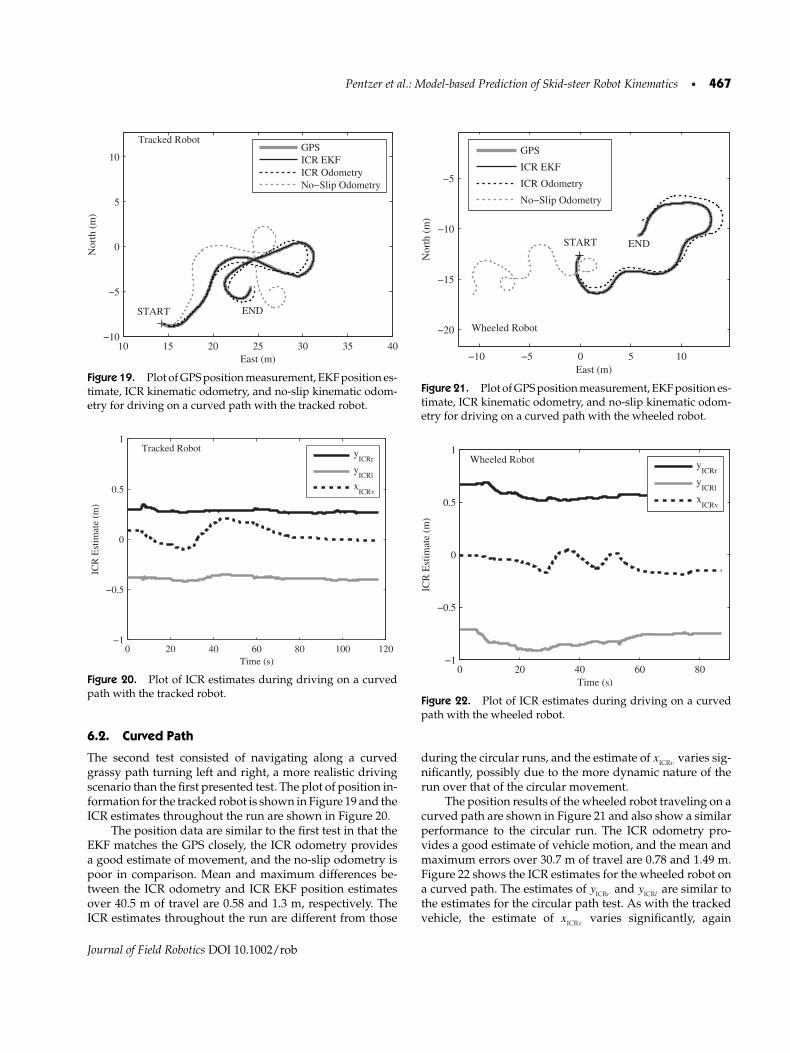
Figure 19. Plot of GPS position measurement, EKF position es-timate, ICR kinematic odometry, and no-slip kinematic odom-etry for driving on a curved path with the tracked robot.

0 20 40 60 80 100 120−1

−0.5

0

0.5

1

Time (s)

ICR

Est

imat

e (m

)

y

ICRr

yICRl

xICRv

Tracked Robot

Figure 20. Plot of ICR estimates during driving on a curvedpath with the tracked robot.

6.2. Curved Path

The second test consisted of navigating along a curvedgrassy path turning left and right, a more realistic drivingscenario than the first presented test. The plot of position in-formation for the tracked robot is shown in Figure 19 and theICR estimates throughout the run are shown in Figure 20.

The position data are similar to the first test in that theEKF matches the GPS closely, the ICR odometry providesa good estimate of movement, and the no-slip odometry ispoor in comparison. Mean and maximum differences be-tween the ICR odometry and ICR EKF position estimatesover 40.5 m of travel are 0.58 and 1.3 m, respectively. TheICR estimates throughout the run are different from those

−10 −5 0 5 10

−20

−15

−10

−5

East (m)

Nor

th (

m)

GPS

ICR EKF

ICR Odometry

No−Slip Odometry

Wheeled Robot

ENDSTART

Figure 21. Plot of GPS position measurement, EKF position es-timate, ICR kinematic odometry, and no-slip kinematic odom-etry for driving on a curved path with the wheeled robot.

0 20 40 60 80−1

−0.5

0

0.5

1

Time (s)

ICR

Est

imat

e (m

)

y

ICRr

yICRl

xICRv

Wheeled Robot

Figure 22. Plot of ICR estimates during driving on a curvedpath with the wheeled robot.

during the circular runs, and the estimate of xICRvvaries sig-

nificantly, possibly due to the more dynamic nature of therun over that of the circular movement.

The position results of the wheeled robot traveling on acurved path are shown in Figure 21 and also show a similarperformance to the circular run. The ICR odometry pro-vides a good estimate of vehicle motion, and the mean andmaximum errors over 30.7 m of travel are 0.78 and 1.49 m.Figure 22 shows the ICR estimates for the wheeled robot ona curved path. The estimates of yICRr

and yICRlare similar to

the estimates for the circular path test. As with the trackedvehicle, the estimate of xICRv

varies significantly, again



−20 −10 0 10 20 30 40−50

−40

−30

−20

−10

0

East (m)

Nor

th (

m)

GPS

ICR EKF

START

END

Tracked Robot

Figure 23. Plot of GPS measured position and EKF positionestimate during a lawnmower search pattern with the trackedrobot.

−0.5 0 0.5 10

5

10

15

20

25

ICR Location (m)

Perc

enta

ge o

f T

ime

at I

CR

Est

imat

e

y

ICRr

yICRl

xICRv

Tracked Robot

Figure 24. Clustering of ICR location estimates during a long-distance run with the tracked robot.

suggesting that the longitudinal location of the ICRs de-pends more on the dynamics than the lateral position.

6.3. Long-distance Traversal

The third segment of testing consisted of driving each robotin a lawnmower search pattern for approximately 1,000 mof travel, as shown for the tracked robot in Figure 23 andthe wheeled robot in Figure 25. The purpose of this testwas to investigate filter performance over a longer timeof operation. After convergence, the ICR location estimates

−30 −20 −10 0 10 20 30

−40

−30

−20

−10

0

East (m)

Nor

th (

m)

GPS

ICR EKF

START

END

Wheeled Robot

Figure 25. Plot of GPS measured position and EKF positionestimate during a lawnmower search pattern with the wheeledrobot.

−1 −0.5 0 0.5 1 1.5

5

10

15

20

25

30

35

ICR Location (m)

Perc

enta

ge o

f T

ime

at I

CR

Est

imat

e

y

ICRr

yICRl

xICRv

Wheeled Robot

Figure 26. Clustering of ICR location estimates during a long-distance run with the wheeled robot.

remain fairly stable throughout the run for each vehicle.This is illustrated in Figure 24 for the tracked robot andFigure 26 for the wheeled robot, where the height of a barrepresents the percentage of total run time during which thefilter estimated a particular ICR location.

The mean error between the ICR EKF and the GPS po-sition solution was 1.8 cm for the tracked robot and 1.6 cmfor the wheeled robot. As expected, the yICR values for thelong-distance run lie outside the robot track/wheel loca-tions, which in local coordinates are ±0.26 m for the trackedrobot and ±0.31 m for the wheeled robot. More slippage is



−10 −5 0 5 10 15 20

−25

−20

−15

−10

−5

0

East (m)

Nor

th (

m)

GPS

ICR EKF

Dropout Start

Dropout End

START

END

Tracked Robot

Figure 27. Test of ICR odometry as a backup system duringGPS dropouts with the tracked robot.

expected to occur with the wheeled robot as the distancebetween the wheels and ICR locations is larger than theanalogous distance on the tracked robot. The motors andbatteries are mounted forward of the longitudinal center ofthe tracked robot, which shifts the center of gravity forwardand accounts for the positive estimated xICRv

location. Thewheeled robot has a very even weight distribution due tothe fact that it consists of two complete systems operatingtogether. This is reflected in the results by the estimated xICRv

staying near 0 m.

6.4. Testing ICR Methods for Robot LocalizationDuring GPS Outages

Because ICR position estimates are quite accurate, they canbe used to localize ground robots in situations in which theGPS, INS, or odometry systems may have outages or errors.Poor GPS solutions and outages are caused by a numberof factors, including multipath signals and sky occlusions.Here a situation is tested in which the ICR EKF is run along-side a traditional GPS-based position estimate: when GPS(or similar position information) is available, this algorithmupdates ICR location estimates. When GPS is unavailable,the ICR kinematic equations are used to propagate move-ment with the most recently learned ICR locations. Theresults of this system are shown for the tracked robot inFigure 27 where three GPS dropouts of 20 s duration areforced to occur. The ICR kinematic equations are used topredict the movement of the robot throughout the GPSdropout and are accurate to within 0.4 m in the first andthird dropout and within 0.65 m in the second dropout. Theaccuracy of the ICR odometry is heavily influenced by themovement of the robot. Higher numbers of turns and also

0 1 2 3 4 50

5

10

15

20

25

30

Error in Odometry Estimate (m)

Perc

enta

ge o

f O

ccur

renc

es

Expected Value of Error 0.89 m

95% of Occurences Below 1.6 m

Tracked Robot

Figure 28. Histogram of open-loop ICR odometry error on thetracked robot after 5 m of travel from each point traversed in alawnmower search pattern.

tighter turns will result in more divergence in the positionestimate.

The performance of the open-loop ICR odometry dur-ing GPS dropouts was further investigated using the lawn-mower search pattern data presented in Figure 23. Usingeach recorded state as a starting location, the position of therobot was estimated forward in time for a set distance. TheICR locations estimated by the onboard filter at the startingpoint were used for the odometry. The resulting positionwas compared with the EKF estimate that utilized GPS andheading measurements for estimation. This analysis wasdone for traversal distances of 1–20 m for both the trackedand wheeled robots.

Examples of the results for individual traversal dis-tances are shown in Figures 28–30 for 5, 10, and 20 mGPS dropouts on the tracked vehicle. The result of the 5 mdropout analysis indicates that the ICR odometry is within1.6 m for 95% of the trials and that the expected error valuebased on a weighted average of the histogram distributionis 0.89 m. For the 10 m GPS dropout, the odometry estimateis within 3.8 m for 95% of the trials and has an expectederror value of 1.6 m. The odometry estimate is within 10 mfor 95% of the trials and has an expected error value of 3.5 mwith a 20 m GPS dropout.

The results for all GPS dropout lengths are summarizedfor the tracked robot in Figure 31 and the wheeled robot inFigure 32. The performance of the ICR and no-slip odome-try is similar up to around 10 m for the tracked robot, butat longer dropout lengths the ICR outperforms the no-slipodometry. With the wheeled vehicle, the ICR odometry es-timate is significantly better than the no-slip odometry fornearly all tested values of dropout length. In fact, for all



0 2 4 6 8 100

2

4

6

8

10

12


Perc

enta

ge o

f O

ccur

renc

es

95% of OccurencesBelow 3.8 m

Expected Value of Error 1.6 m Tracked Robot

Figure 29. Histogram of open-loop ICR odometry error on thetracked robot after 10 m of travel from each point traversed ina lawnmower search pattern.

0 5 10 15 200

1

2

3

4

5

6

7


Perc

enta

ge o

f O

ccur

renc

es

95% of OccurencesBelow 10.4 m

Expected Value of Error 3.5 m

Tracked Robot

Figure 30. Histogram of open-loop ICR odometry error on thetracked robot after 20 m of travel from each point traversed ina lawnmower search pattern.

dropout lengths greater than 6 m, both of the recorded ICRerror values lie below the expected value of error for theno-slip odometry, indicating that the ICR algorithm per-forms much better than the no-slip on the wheeled robot.The improvement of the ICR odometry over the no-slipodometry between the tracked and wheeled vehicle is mostlikely due to increased slip with the wheeled robot. Whilethe tracked and wheeled robots are similar in width, theestimated yICRr

and yICRllocations for the wheeled robot are

much larger than those for the tracked robot, indicating in-creased slip with the wheeled vehicle.

0 5 10 15 200

5

10

15

20

25

30

35

40

GPS Dropout Length (m)

Err

or in

Odo

met

ry (

m)

95% of Trials Within Error − ICR

Expected Value of Error − ICR

95% of Trials Within Error − No−Slip

Expected Value of Error − No−Slip

Tracked Robot

Figure 31. Summary of open-loop ICR odometry error on thetracked robot for 1–20 m of travel from each point traversed ina lawnmower search pattern.

0 5 10 15 200

5

10

15

20

25

30

35

40


Err

or in

Odo

met

ry (

m)





Wheeled Robot

Figure 32. Summary of open-loop ICR odometry error on thewheeled robot for 1–20 m of travel from each point traversedin a lawnmower search pattern.

The no-slip odometry trajectories in Figures 19 and 21indicate that larger errors would be expected for no-slipodometry than appear in Figures 31 and 32. However, theshorter runs in Figures 19 and 21 consist of many more turnsat higher frequencies than the lawnmower pattern used inthe GPS dropout analysis. During cornering maneuvers,the ICR odometry is much better than no-slip, as shown inFigure 33, but during straight sections the two odom-etry methods are very similar, as shown in Figure 34.For shorter GPS dropout lengths, the lawnmower pattern



−30 −20 −10 0 10 20 30 40−50

−40

−30

−20

−10

0

10

East (m)

Nor

th (

m)

GPSICR OdometryNo−Slip Odometry

Tracked Robot

Figure 33. Two examples of ICR and no-slip odometry perfor-mance over 15 m distances with the tracked robot.

−30 −20 −10 0 10 20 30−50

−40

−30

−20

−10

0

10

East (m)

Nor

th (

m)

GPSICR OdometryNo−Slip Odometry

Wheeled Robot

Figure 34. Two examples of ICR and no-slip odometry perfor-mance over 15 m distances with the wheeled robot.

appears mainly as a series of short straight sections with fewcurves, allowing the no-slip odometry to perform compara-bly to the ICR with the tracked vehicle. For longer dropouts,the corners become more apparent, and the ICR begins tooutperform the no-slip odometry. For the wheeled robot,the increased amount of slippage causes the no-slip odome-try to become very inaccurate with only small turns, whichaccounts for the large improvement seen in Figure 32 withthe ICR over the no-slip odometry. In summary, a skid-steervehicle traveling in straight lines would not benefit signif-icantly from ICR odometry, but improvements to motionestimation will be seen when using ICR odometry with arobot operating on any path requiring it to turn.

−20 −10 0 10 20 30

−40

−30

−20

−10

0

East (m)

Nor

th (

m)

GPSICR EKF

Tracked RobotSTART

END

Figure 35. Plot of measured GPS position and EKF positionestimate when operating without RTK GPS corrections.

6.5. Testing with a Conventional GPS Solution

The previous work utilized an RTK GPS system for positionmeasurement. This is a specialized system that requires localcorrections that may not be available in all situations. Threelaps of the long-distance course presented in Section 6.3were repeated using the tracked vehicle with the local GPScorrection station turned off. Thus, the GPS system utilizedonly the less accurate satellite-based corrections from thewide-area augmentation system (WAAS). The GPS manu-facturer provides an estimate of 0.30 m rms horizontal po-sition accuracy when using WAAS. The resulting positionplot of the GPS measured and estimated position is shownin Figure 35, and the estimated ICR locations throughout therun are summarized in Figure 36. The mean velocity of therobot was 0.7 m/s, with a standard deviation of 0.15 m/s.The ICR location estimates have means and standard de-viations of yICRr

= 0.41 m, σICRr= 0.08 m; yICRl

= −0.57 m,σICRl

= 0.04 m; and xICRv= 0.3 m, σICRv

= 0.06 m.These values of ICR locations are slightly different from

those found in the long-distance traversal section. This ismost likely due to changing terrain properties: the long-distance traversal tests of Section 6.3 were performed inlate spring when the grass on the surface was three to fourinches tall and very lush, while the testing without RTKcorrections was performed in early fall when the grass wasone to two inches tall and very dry.

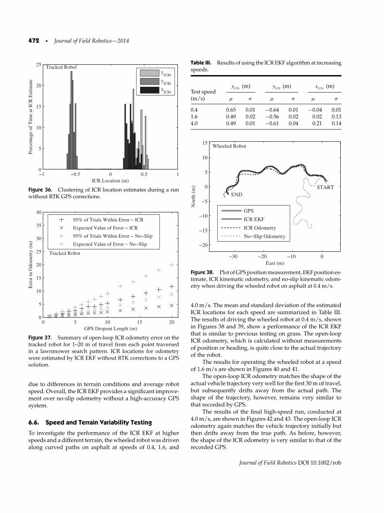
The GPS outage analysis of Section 6.4 was repeatedon the traversal data without RTK corrections. The re-sults, shown in Figure 37, indicate that with a standardGPS, the estimated ICR locations still provide improvedodometry over a no-slip estimate. The improvement isgreater than that of the long-distance traversal test shown inFigure 31, but more detailed comparisons may be difficult



−1 −0.5 0 0.5 10

5

10

15

20

25

ICR Location (m)

Perc

enta

ge o

f T

ime

at I

CR

Est

imat

e

y

ICRr

yICRl

xICRv

Tracked Robot

Figure 36. Clustering of ICR location estimates during a runwithout RTK GPS corrections.

0 5 10 15 200

5

10

15

20

25

30

35

40


Err

or in

Odo

met

ry (

m)





Tracked Robot

Figure 37. Summary of open-loop ICR odometry error on thetracked robot for 1–20 m of travel from each point traversedin a lawnmower search pattern. ICR locations for odometrywere estimated by ICR EKF without RTK corrections to a GPSsolution.

due to differences in terrain conditions and average robotspeed. Overall, the ICR EKF provides a significant improve-ment over no-slip odometry without a high-accuracy GPSsystem.

6.6. Speed and Terrain Variability Testing

To investigate the performance of the ICR EKF at higherspeeds and a different terrain, the wheeled robot was drivenalong curved paths on asphalt at speeds of 0.4, 1.6, and

Table III. Results of using the ICR EKF algorithm at increasingspeeds.

yICRr(m) yICRl

(m) xICRv(m)

Test speed(m/s) μ σ μ σ μ σ

0.4 0.65 0.01 −0.64 0.01 −0.04 0.011.6 0.49 0.02 −0.56 0.02 0.02 0.134.0 0.49 0.01 −0.61 0.04 0.21 0.14

−30 −20 −10 0

−20

−15

−10

−5

0

5

10

15

East (m)

Nor

th (

m)

GPS

ICR EKF

ICR Odometry

No−Slip Odometry

STARTEND

Wheeled Robot

Figure 38. Plot of GPS position measurement, EKF position es-timate, ICR kinematic odometry, and no-slip kinematic odom-etry when driving the wheeled robot on asphalt at 0.4 m/s.

4.0 m/s. The mean and standard deviation of the estimatedICR locations for each speed are summarized in Table III.The results of driving the wheeled robot at 0.4 m/s, shownin Figures 38 and 39, show a performance of the ICR EKFthat is similar to previous testing on grass. The open-loopICR odometry, which is calculated without measurementsof position or heading, is quite close to the actual trajectoryof the robot.

The results for operating the wheeled robot at a speedof 1.6 m/s are shown in Figures 40 and 41.

The open-loop ICR odometry matches the shape of theactual vehicle trajectory very well for the first 30 m of travel,but subsequently drifts away from the actual path. Theshape of the trajectory, however, remains very similar tothat recorded by GPS.

The results of the final high-speed run, conducted at4.0 m/s, are shown in Figures 42 and 43. The open-loop ICRodometry again matches the vehicle trajectory initially butthen drifts away from the true path. As before, however,the shape of the ICR odometry is very similar to that of therecorded GPS.



−1 −0.5 0 0.5 1 1.5

10

20

30

40

50

ICR Location (m)

Perc

enta

ge o

f T

ime

at I

CR

Est

imat

e

y

ICRr

yICRl

xICRv

Wheeled Robot

Figure 39. Clustering of ICR location estimates when drivingthe wheeled robot on asphalt at 0.4 m/s.

−40 −20 0 20−30

−20

−10

0

10

20

30

East (m)

Nor

th (

m)


Wheeled Robot

START

END


Comparing Figures 38, 40, and 42, the variance in theestimate of xICRv

increases as the vehicle speed increases.However, the estimates of yICRr

and yICRlremain tightly clus-

tered around similar values for all three runs. Increasedvariance in xICRv

occurs at larger lateral velocities caused byhigher speeds. In these situations, larger track/tire forcesare required due to dynamics not modeled in the ICR EKF.The slip angle of a moving vehicle, which relates the actualdirection of travel to the direction it is pointing for skid-steer vehicles, is for small slip values proportional to the

−1 −0.5 0 0.5 10

10

20

30

40

50

60

70

ICR Location (m)

Perc

enta

ge o

f T

ime

at I

CR

Est

imat

e

y

ICRr

yICRl

xICRv

Wheeled Robot


−60 −40 −20 0 20 40 60−40

−20

0

20

40

60

East (m)

Nor

th (

m)

GPS

ICR EKF

ICR Odometry

No−Slip Odometry

Wheeled Robot

STARTEND


track/tire force (Wong, 2008). A tighter turn at high speedwill have a larger slip angle, and therefore larger lateral ve-locity, which is related to xICRv

as shown in Eq. (9). At higherspeeds, the assumption that the xICRv

location is constant inthe ICR EKF model breaks down. A comparison of the abso-lute difference in the ICR EKF north-east position estimateand the measurement of vehicle position provided by theGPS is shown in Figure 44. At low speeds, the difference iswithin the accuracy of the RTK GPS, and, as expected due tothe difficulty in estimating ICR locations, the error increasesat higher speeds. It was quite difficult to manually operate



−1 −0.5 0 0.5 10

5

10

15

20

25

30

35

ICR Location (m)

Perc

enta

ge o

f T

ime

at I

CR

Est

imat

e

y

ICRr

yICRl

xICRv

Wheeled Robot


0 20 40 60 80 1000

0.05

0.1

0.15

0.2

0.25

0.3

0.35

Percentage of Mission Completion

Dif

fere

nce

in I

CR

EK

F an

d G

PS P

ositi

on (

m)

0.4 m/s1.6 m/s4.0 m/s

Figure 44. Comparison of the difference in ICR EKF positionestimate and measurement from the RTK GPS system.

the wheeled robot such that it followed a curved path at4.0 m/s. The turning ability of the vehicle is limited at suchspeeds, so avoiding obstacles in the test area becomes a sig-nificant issue. The tracked vehicle has a maximum speedof approximately 1 m/s in its current configuration, so noadditional high-speed testing was performed with it.

Future work in speed variability testing will focus onthe area of utilizing the ICR kinematic model for trajec-tory control of skid-steer vehicles. This will enable repeatedtraversal of set paths at varying speeds, which is currentlydifficult to do at higher speeds. A direct comparison ofICR EKF performance on the same path type will then bepossible.

7. CONCLUSIONS AND FUTURE WORK

This paper presents an EKF algorithm capable of learningthe ICR locations of a skid-steer ground robot during oper-ation. An ICR-based kinematic model of skid-steer move-ment using track velocity inputs is used to model the sys-tem, and measurements of position and heading are used toupdate the state and enable learning of ICR locations. Thealgorithm was first developed in a simulation, where it wasfound that modification of the ICR kinematics to ensure thecorrect sign is necessary for filter convergence in the pres-ence of noise. Further investigation showed that the filteris more sensitive to noise than bias on the track velocityinputs.

The main contribution of this paper is an algorithm thatlearns ICR locations relating input track or wheel speedto skid-steer vehicle motion without prior knowledge ofterrain type or vehicle configuration. ICR locations remainrelatively constant for skid-steer vehicle operation at lowspeeds on hard, flat terrain regardless of vehicle motion.This allows estimated ICR locations to be used for odometryor to map desired vehicle motion, such as forward speedand angular rate, to required track or wheel speeds. ICRlocations have also been successfully used to model powerusage in skid-steer wheeled and tracked vehicles (Moraleset al., 2009). Estimation of ICR positions during operationenables identification and prediction of skid-steer powerusage without prior knowledge of terrain properties.

The algorithm has undergone substantial field-testingon a tracked skid-steer robot developed at The PennsylvaniaState University and a commercial skid-steer wheeled robot.Results presented in this work show that ICR locations es-timated by the ICR EKF algorithm provide good predic-tions of robot movement, and that assuming no-slip whenperforming odometry with skid-steer vehicles gives com-paratively poor position estimates. ICR estimates generallyconverge within 5–15 s of operating the vehicle dependingon the type of movement the robot performs. Overall, theperformance of the ICR EKF was quite good consideringno prior knowledge of robot design or terrain parameterswere needed. Over a 40.5 m traversal, ICR odometry usinglearned ICR locations predicted positions with a mean errorof 0.58 m with the tracked robot when using the most recentICR estimates at each time step. The ICR EKF algorithm wastested with both robots on separate 1,000 m runs and pro-vided estimates of position within 2 cm of GPS on average.This accuracy is expected and not a major contribution fromthe filter because the ICR EKF receives GPS measurementsat 20 Hz. Rather, the real-time estimates of ICR locationand their use in accurate odometry and real-time estima-tion of wheel slip in the case of GPS dropouts are the maincontributions of the algorithm. ICR estimates during thelong-distance test cluster around values of yICRr

= 0.38 m,yICRl

= −0.42 m, and xICRv= 0.16 m for the tracked robot,

and yICRr= 0.64 m, yICRl

= −0.76 m, and xICRv= −0.04 m for



the wheeled robot. The vehicles are similar in width, sothe larger yICR values for the wheeled robot indicate largeramounts of slip during operation than with the trackedrobot. The longitudinal location, xICRv

, seems to vary morethan the lateral locations for both robots, and it remainedconstant during testing only for the circular run, where thedynamics of the vehicle are fairly constant. Further testingof the wheeled robot at speeds of 1.6 and 4.0 m/s showedincreasing variance in the estimate of xICRv

for increasing ve-hicle speeds. The increased variance is thought to be causedby increased lateral slippage due to unmodeled dynamicsat higher speeds.

There are many applications for continued work in thisarea. An obvious one demonstrated in this paper is that ofa backup to GPS positioning. Loss of GPS signal is a com-mon occurrence in ground robotics, and the ICR EKF iswell suited to learn parameters in the background and stepin as needed to estimate movement in the absence of GPS.Dropouts of the GPS position solution for various lengths ofvehicle traversal were simulated using recorded data. Re-sults indicated that ICR odometry on the tracked robot isaccurate to within 1.6 m for a 5 m GPS dropout, 3.8 m fora 10 m GPS dropout, and 10 m for a 20 m GPS dropout for95% of trials. This analysis was extended to the wheeledrobot and GPS dropout lengths from 1 to 20 m. The resultsshowed that vehicles with larger amounts of slippage willbenefit more from ICR odometry than no-slip odometry.For example, the wheeled robot in this work slipped sig-nificantly more than the tracked robot and therefore hadlarger amounts of improvement with ICR odometry. TheICR estimates produced open-loop prediction errors on thewheeled robot that are roughly 18% of the distance trav-eled, versus 45% for the no-slip model. On the trackedrobot, ICR odometry produced open-loop prediction errorsof roughly 17% of the distance traveled, versus 22% forthe no-slip model. For both robots there is a significant im-provement in the accuracy of kinematic prediction with ICRodometry compared to using the same measurements witha no-slip model. Our results show that these improvementswill be most pronounced on paths with large numbers ofcurves.

Previous work in odometry for skid-steer vehicles hasshown estimation accuracies of 2% of distance traveled orbetter (Rogers-Marcovitz et al., 2012; Yi et al., 2009), but suchalgorithms relied on empirically determined constants re-lated to terrain and/or vehicle configuration and high costsensors not typically found on ground mobile robots. Thealgorithm presented in this work provides less accurateodometry predictions, but is easily adapted to tracked orwheeled skid-steer vehicles without extensive vehicle mod-eling or calibration maneuvers.

Another area of continued research is testing of theICR EKF at different speeds and path types. The scope oftesting will be determined in part by concurrent researchidentifying the operational envelope of teleoperated skid-

steer vehicles when driven by experienced operators. A sig-nificant ICR EKF assumption is that the robots operate atlow speeds, below 1 m/s, and this work has quantified toa limited extent how position estimates degrade with in-creasing speed of operation for current skid-steer robots upto 4 m/s for a wheeled platform. It is reasonable to expectthat teleoperated skid-steer vehicles will continue to oper-ate at low speeds the majority of the time due to difficultiesin perceiving and manipulating the environment duringoperation. However, future work remains to develop sim-ple models for accurate robot pose estimation during high-slip and/or high-force ground maneuvering that is likely atspeeds higher than 4 m/s.

ACKNOWLEDGMENTS

This work was supported by the Exploratory and Founda-tional Research Program, administered by the Applied Re-search Laboratory, The Pennsylvania State University. Noofficial endorsement should be inferred.

REFERENCES

Almeida, J., & Santos, V. M. (2013). Real time egomotion of anonholonomic vehicle using lidar measurements. Journalof Field Robotics, 30(1), 129–141.

Angelova, A., Matthies, L., Helmick, D., & Perona, P. (2006).Slip prediction using visual information. In Proceedingsof Robotics Science and Systems Conference.

Anousaki, G., & Kyriakopoulos, K. J. (2004). A dead-reckoningscheme for skid-steered vehicles in outdoor environments.In Proceedings of the 2004 IEEE International Conferenceon Robotics and Automation (pp. 580–585).

Botterill, T., Mills, S., & Green, R. (2011). Bag-of-words-driven,single-camera simultaneous localization and mapping.Journal of Field Robotics, 28(2), 204–226.

Burke, M. (2012). Path-following control of a velocity con-strained tracked vehicle incorporating adaptive slip es-timation. In Proceedings of the 2012 IEEE InternationalConference on Robotics and Automation (pp. 97–102).

Chuy, O., Jr., Collins, E., Jr., Yu, W., & Ordonez, C. (2009). Powermodeling of a skid steered wheeled robotic ground vehicle.In Proceedings of the 2009 IEEE International Conferenceon Robotics and Automation (pp. 4118–4123).

Dar, T. M., & Longoria, R. G. (2010). Slip estimation for small-scale robotic tracked vehicles. In Proceedings of the 2010American Control Conference (pp. 6816–6821).

Ferretti, G., & Girelli, R. (1999). Modelling and simulation of anagricultural tracked vehicle. Journal of Terramechanics, 36,139–158.

Kozlowski, K., & Pazderski, D. (2004). Modeling and control ofa 4-wheel skid-steering mobile robot. International Journalof Applied Math and Computer Science, 14(4), 477–496.



Kuo, B., & Golnaraghi, F. (2003). Automatic control systems,8th ed. Hoboken, NJ: John Wiley & Sons, Inc.

Lambert, A., Furgale, P., Barfoot, T. D., & Enright, J. (2012).Field testing of visual odometry aided by a sun sensor andinclinometer. Journal of Field Robotics, 29(3), 426–444.

Le, A. T., Rye, D. C., & Durrant-Whyte, H. F. (1997). Estimationof track-soil interactions for autonomous tracked vehicles.In Proceedings of the 1997 IEEE International Conferenceon Robotics and Automation (pp. 1388–1393).

Marks, T. K., Howard, A., Bajracharya, M., Cottrell, G. W., &Matthies, L. H. (2009). Gamma-slam: Visual slam in un-structured environments. Journal of Field Robotics, 26(1),26–51.

Martınez, J. L., Mandow, A., Morales, J., Pedraza, S., & Garcıa-Cerezo, A. J. (2005). Approximating kinematics for trackedmobile robots. The International Journal of Robotics Re-search, 24(10), 867–878.

Milella, A., Reina, G., & Siegwart, R. (2006). Computer vi-sion methods for improved mobile robot state estima-tion in challenging terrains. Journal of Multimedia, 1(7),49–61.

Moosavian, S. A. A., & Kalantari, A. (2008). Experimental slipestimation for exact kinematics modeling and control ofa tracked mobile robot. In 2008 IEEE/RSJ InternationalConference on Intelligent Robots and Systems (pp. 95–100).

Morales, J., Martınez, J. L., Mandow, A., Garcıa-Cerezo, A. J., &Pedraza, S. (2009). Power consumption modeling of skid-steer tracked mobile robots on rigid terrain. IEEE Transac-tions on Robotics, 25(5), 1098–1108.

Nister, D., Naroditsky, O., & Bergen, J. (2004). Visual odom-etry. In Proceedings of the 2004 IEEE Computer SocietyConference on Computer Vision and Pattern Recognition.

Quigley, M., Gerkey, B., Conley, K., Faust, J., Foote, T., Leibs,J., Berger, E., Wheeler, R., & Ng, A. (2009). ROS: An open-source robot operating system. In Proceedings of the 2009IEEE International Conference on Robotics and Automa-tion Workshop on Open Source Robotics.

Robotic Systems Joint Project Office (2012). Unmanned groundsystems roadmap.

Rogers-Marcovitz, F., George, M., Seegmiller, N., & Kelly, A.(2012). Aiding off-road inertial navigation with high per-formance models of wheel slip. In Proceedings of the 2012IEEE/RSJ International Conference on Intelligent Robotsand Systems (pp. 215–222).

Song, X., Seneviratne, L. D., & Althoefer, K. (2011a). A Kalmanfilter-integrated optical flow method for velocity sensingof mobile robots. IEEE/ASME Transactions on Mechatron-ics, 16(3), 551–563.

Song, X., Seneviratne, L. D., & Althoefer, K. (2011b). Slip param-eter estimation for tele-operated ground vehicles in slip-pery terrain. Proceedings of the Institution of MechanicalEngineers, Part I: Journal of Systems and Control Engi-neering, 225(6), 814–830.

Vinh Ha, X., Ha, C., & Lee, J. (2013). Fuzzy vector field orien-tation feedback control-based slip compensation for tra-jectory tracking control of a four track wheel skid-steeredmobile robot. International Journal of Advanced RoboticSystems, 10, 1.

Wang, D., & Low, C. B. (2008). Modeling and analysis of skid-ding and slipping in wheeled mobile robots: Control de-sign perspective. IEEE Transactions on Robotics, 24(3),676–687.

Ward, C. C., & Iagnemma, K. (2008). A dynamic-model-basedwheel slip detector for mobile robots on outdoor terrain.IEEE Transactions on Robotics, 24(4), 821–831.

Wong, J. (2008). Theory of Ground Vehicles, 4th ed. John Wileyand Sons.

Wong, J. Y., & Chiang, C. F. (2001). A general theory for skidsteering of tracked vehicles on firm ground. Proceedingsof the Institution of Mechanical Engineers, Part D: Journalof Automobile Engineering, 215(3), 343–355.

Yi, J., Song, D., Zhang, J., & Goodwin, Z. (2007a). Adaptivetrajectory tracking control of skid-steered mobile robots.In Proceedings of the 2007 IEEE International Conferenceon Robotics and Automation (pp. 10–14).

Yi, J., Wang, H., Zhang, J., Song, D., Jayasuriya, S., & Liu, J.(2009). Kinematic modeling and analysis of skid-steeredmobile robots with applications to low-cost inertial-measurement-unit-based motion estimation. IEEE Trans-actions on Robotics, 25(5), 1087–1097.

Yi, J., Zhang, J., Song, D., & Jayasuriya, S. (2007b). IMU-basedlocalization and slip estimation for skid-steered mobilerobots. In Proceedings of the 2007 IEEE/RSJ InternationalConference on Intelligent Robots and Systems (pp. 2845–2850).

Zweiri, Y. H., Seneviratne, L. D., & Althoefer, K. (2003). Mod-elling and control of an unmanned excavator. Proceedingsof the Institution of Mechanical Engineers , Part I : Journalof Systems and Control Engineering, 217, 259–274.


Date post:	25-Dec-2015
Category:	Documents
Upload:	abner-chavez
View:	213 times
Download:	1 times

Pentzer Et Al-2014-Journal of Field Robotics

Documents