Perception & evaluation of audio quality in music production Wilson, AD and Fazenda, BM Title Perception & evaluation of audio quality in music production Authors Wilson, AD and Fazenda, BM Type Article URL This version is available at: http://usir.salford.ac.uk/30255/ Published Date 2013 USIR is a digital collection of the research output of the University of Salford. Where copyright permits, full text material held in the repository is made freely available online and can be read, downloaded and copied for non-commercial private study or research purposes. Please check the manuscript for any further copyright restrictions. For more information, including our policy and submission procedure, please contact the Repository Team at: [email protected].
Transcript
Perception & evaluation of audio quality in music production
Wilson, AD and Fazenda, BM
Title Perception & evaluation of audio quality in music production
Authors Wilson, AD and Fazenda, BM
Type Article
URL This version is available at: http://usir.salford.ac.uk/30255/
Published Date 2013
USIR is a digital collection of the research output of the University of Salford. Where copyright permits, full text material held in the repository is made freely available online and can be read, downloaded and copied for noncommercial private study or research purposes. Please check the manuscript for any further copyright restrictions.
For more information, including our policy and submission procedure, pleasecontact the Repository Team at: [email protected].
A dataset of audio clips was prepared and audio quality assessedby subjective testing. Encoded as digital signals, a large amountof feature-extraction was possible. A new objective metric is pro-posed, describing the Gaussian nature of a signal’s amplitude dis-tribution. Correlations between objective measurements of themusic signals and the subjective perception of their quality werefound. Existing metrics were adjusted to match quality perception.A number of timbral, spatial, rhythmic and amplitude measures, inaddition to predictions of emotional response, were found to be re-lated to the perception of quality. The emotional features werefound to have most importance, indicating a connection betweenquality and a unified set of subjective and objective parameters.
1. INTRODUCTION
A single, consistent definition for quality has not yet been offered,however, for certain restricted circumstances, ‘quality’ has an un-derstood meaning when applied to audio. Measurement techniquesexist for the assessment of audio quality, such as [1] and [2], how-ever such standards typically apply to the measurement of qualitywith reference to a golden sample; what is in fact being ascertainedis the reduction in perceived quality due to destructive processes,such as the effects of compression codecs, in which the audio beingevaluated is a compressed version of the reference and the deteri-oration in quality is measured [3].
Such descriptions would not strictly apply to the evaluation ofquality in musical recordings. This study is concerned with theaudio quality of ‘produced’ commercial music where there is nofixed reference and quality is evaluated by comparison with allother samples heard. This judgement is based on both subjectiveand objective considerations.
In systems where objective measurement is possible, there isstill disagreement regarding which parameters contribute to qualityand the manner of their contribution. The work of Toole indicatesthat, with loudspeakers, even a measure as trivial as the on-axisamplitude response does not have a simple relationship to quality[4]. Toole suggests evidence of many secondary factors influenc-ing listener preference, even based on geography. For example, [5]describes a specific studio monitor as having a ‘European’ tone,citing a consistent, subjective evaluation leading to this descrip-tion.
With music being described by Gurney as the ‘peculiar delightwhich is at once perfectly distinct and perfectly indescribable’[6],this use of language is typical in audio and does present some prob-lems. Lacking a solid definition for audio quality, each listener can
apply their own criteria, making it highly subjective.[7] describes a series of subjective parameters (including spa-
tial impression and tonality) and suggests applicable measurementmethodologies. The concept of the existence of an ideal amountof a given signal parameter to yield maximal subjective qualityratings for a given piece of music is one that will be explored.
If quality is highly subjective the aspects of the subject whichare of influence can be investigated. [8] found that an expert groupof music professionals was able to distinguish various recordingmedia from one another, based on their subjective audio qualityratings of classical music recordings. While a CD and cassettedisplayed a distinct difference in quality, formats of higher fidelitythan CD were not rated significantly higher than the CD. The ex-pertise of the listener is therefore thought to be a factor in quality-perception, due to ability to detect technical flaws.
In summary, audio quality, as applied to music recordings,is predicted to be based on both subjective and objective mea-sures. This paper will investigate both aspects using independentmethodologies, and subsequently attempt to determine what corre-lations exist and how the subjective and objective evaluations canbe linked, to lead towards a quality-prediction model.
2. METHODOLOGY
The hypotheses under test are as follows:1. There are noticeable differences in quality between samples2. Listener training has an influence on perception of quality3. Familiarity with a sample is related to how much it is liked4. Quality is related to one or more objective signal parameters
2.1. Subjective Testing
To obtain subjective measures of the audio signals a listening testwas designed in which subjects listened to a series of audio clipsand answered simple questions on their experience.
Basic information about the subject was gathered so that re-sults could be analysed based on demographics. The age and sexof each subject was recorded. In addition, subjects were asked toidentify themselves as either ‘audio expert’, ‘musician’ or ‘noneof the above’. This last category is used as a control group hereinreferred to as the naïve group. Subjects in this category wouldideally not possess professional knowledge of acoustics or audioengineering and lack any above-average musical ability. Subjectswere given a short briefing in order to ensure the questions wereunderstood. For each audition the subject was asked the questionsin Table 1, designed to investigate the hypotheses under test.
DAFX-1
Proc. of the 16th Int. Conference on Digital Audio Effects (DAFx-13), Maynooth, Ireland, September 2-5, 2013
Proc. of the 16th Int. Conference on Digital Audio Effects (DAFx-13), Maynooth, Ireland, September 2-6, 2013
Table 1: Questions in subjective test
Question AnswersHow familiar are you with thissong?
Not, Somewhat orVery familiar
Please rate this Song 1→ 5 star scalePlease rate the Sound Quality ofthis sample
1→ 5 star scale
2.1.1. Audio Selection
All audio samples were 16-bit, 44.1kHz stereo PCM files. 55 sam-ples were used, each a 20 second segment of the song centeredaround the second chorus (where possible) with a one second fade-in and fade-out. This forecast the test duration at 20-25 minutes.Based on the guidelines described in [9], listener fatigue was con-sidered negligible. The audio selection process was influenced bythe test hypotheses. As familiarity was investigated, there neededto be a number that were unfamiliar to all and some familiar toall. To achieve this, six songs by unsigned Irish artists were used.The bulk of samples used were from 1972 to 2012, with two 1960ssamples, and was predominately pop and rock styles.
2.1.2. Test Delivery
The listening test was delivered using a MATLAB script, whichdisplays text, plays audio and receives user input. Controlled teststook place in the listening room at University Of Salford. Theroom has been designed for subjective testing and meets the re-quirements of ITU-R BS. 1116-1, with a background noise levelof 5.7dBA [10]. While the test ran on a laptop computer subjectswere seated at a displaced monitor and keyboard, minimising dis-tractions as well as reducing fan noise from the computer. Audiowas delivered using Sennheiser HD800 headphones and the orderof playback was randomised for each subject.
Unlike methods described in Section 1, this experiment con-tains no reference for what constitutes highest or lowest quality. Inthis case, what is being tested is that which the subject does natu-rally, listening to music. In more rigorously-controlled testing withmodified stimuli, there is a risk of gathering unnatural responsesto unnatural stimuli. In order to test normal listening experiences,each audition was unique and the audio had not been treated inany way, other than loudness equalisation to mimic modern broad-cast standards or programs such as Spotify. Loudness levels werecalculated using the model described in [11]. These predictionsagreed well with in-situ measurements performed using a Brüel &Kjær Head And Torso Simulator (HATS) and sound level meter.For testing, samples were auditioned at an average listening levelof 84dBA, measured using the HATS and sound level meter.
Additional subjects were tested in less controlled circumstances,outside of the listening room, using Sennheiser HD 25-1 II head-phones. A small number of subjects were tested in both controlledand uncontrolled circumstances and displayed a high level of con-sistency, permitting further uncontrolled tests, most of which tookplace in quiet locations at NUI Maynooth and Trinity College Dublin.
2.2. Objective Measures
In order to characterise the audio signals the features in Table 2were extracted from each sample. Feature-extraction was aided bythe use of the MIRtoolbox [12].
Table 2: Features used in objective analysis.
Feature DescriptionCrest factor Ratio of peak amplitude to rms amplitude
(in dB)Width 1 - (cross-correlation between left and right
channels of the stereo signal, at a time offsetof zero samples)
Rolloff Frequency at which 85% of spectral energylies below[13]
Harsh energy Fraction of total spectral energy containedwithin 2k-5kHz band
LF energy Fraction of total spectral energy containedwithin 20-80Hz band
Tempo Measured in beats per minuteGauss See Section 2.2.1Happy Prediction of emotional response[14]Anger Prediction of emotional response[14]
Happy and Anger were chosen from a set of five classes, in-cluding Sadness, Fear and Tenderness. The latter three were re-jected due to weak correlation with quality ratings obtained.
Rolloff describes the extent of the high frequencies and theoverall bandwidth, especially when combined with LF energy, rep-resenting the band reproduced by a typical studio subwoofer, al-though this could extend to 100 or 120Hz in some units. Variousranges were compared to quality ratings and the 20-80Hz rangewas found to be most highly correlated.
Harsh energy was based on author experience and the accountsof mix engineers, where this range was said to imbue a ‘cheap’,‘harsh’, ‘luxurious’ or ‘smooth’ character. Again, various bandswere compared to quality ratings and 2k-5kHz was found to bemost highly correlated.
2.2.1. Gauss - A Measure of Audible Distortion
The classic model of the amplitude distribution of digital audio isa modified Gaussian probability mass function (PMF) with zero-mean. Note: ‘histogram’, ‘probability density function’ and ‘PMF’are often used interchangeably but the unique distinctions are usedhere. Most commercially-released music prior to the mid-1990sadheres to this model, particularly when there is sufficient dynamicrange and the mix consists of many individual elements.
Hard-limiting becomes a feature of the PMF with the onsetof the ‘loudness war’ [15], where the extreme amplitude levels as-sume higher probabilities, sometimes exceeding the zero-amplitudeprobability to become the most probable levels.
A more recent phenomenon has been the presence of widerpeaks in the interim values, as seen in Figure 1b, to avoid clippingas described above. This can be caused by a number of issues,such as the mastering of mixes already limited and the limiting ofindividual elements in the mix, such as the drums. Reports suggestit is not uncommon in modern audio productions to use multiplestages of limiting in the mix process to prepare for the limiting itwill receive during the mastering process [16].
The PMF of each audio signal was analysed to provide fea-tures associated with audible distortion. Hard-limiting and dy-namic range compression have been studied in relation to listenerpreference [17]. Since these parameters are encompassed by thePMF, this study attempts to gather them into a higher-level fea-
DAFX-2
Proc. of the 16th Int. Conference on Digital Audio Effects (DAFx-13), Maynooth, Ireland, September 2-5, 2013
Proc. of the 16th Int. Conference on Digital Audio Effects (DAFx-13), Maynooth, Ireland, September 2-6, 2013
−1 −0.5 0 0.5 10
500
1000
1500f = Histogram
Normalised Sample Amplitude
Ave
rage
Occ
uran
ces
per
seco
nd
−1 −0.5 0 0.5 10
20
40
60
80
100
120
140
160
180
f prime
x
dy/d
x
r2 = 0.9988
DataSmoothedfitted curve
(a) Tori Amos - ‘Crucify’ - 1991
−1 −0.5 0 0.5 10
100
200
300
400
500
600
f = Histogram
Normalised Sample Amplitude
Ave
rage
Occ
uran
ces
per
seco
nd
−1 −0.5 0 0.5 1
0
10
20
30
40
50
f prime
x
dy/d
x
r2 = 0.4026
DataSmoothedfitted curve
(b) Amy Winehouse - ‘Rehab’ - 2006
Figure 1: Depiction of Gauss feature
ture. The histogram was evaluated using 201 bins, providing agood trade-off between runtime, accuracy and clarity of visualisa-tion. In order to evaluate the shape of the distribution, particularlythe slope and the presence of any localised peaks, the first derivatewas determined. For the ideal distribution this had a Gaussian form(see Figure 1a) so the r2 of a Gaussian fit was calculated for eachsample. This was used as a feature describing loudness, dynamicrange and related audible distortions, referred to as ‘Gauss’.
3. RESULTS
The total number of subjects tested was 24; 9 female and 15 male.Expertise was 12 expert, 5 musician and 7 neither. The mean agewas 27 years. With 55 audio samples and 24 subjects, 1320 audi-tions were gathered and analysis was performed on this dataset.
The results of a 3-way ANOVA, shown in Table 3, show thateach main effect is significant (p < 0.05), for quality and like,in addition to a significant second-level interaction between exper-tise and familiarity for quality and two second-level interactions
3.2 3.4 3.6 3.8
Naive
Musician
Expert
1−way ANOVA − Quality, grouped by Expertise
Quality rating
(a) 1-way ANOVA: Mean Quality,grouped by subject group
20 22 24 26 28
Naive
Musician
Expert
One−way ANOVA − TimeTaken grouped by Expertise
Time Taken per sample (s)
(b) 1-way ANOVA: Time Taken,grouped by subject group
Figure 2: Results of subjective test
for like (Sample/Familiar and Expertise/Familiar). To investigatefurther, one-way ANOVA tests were performed with post-hoc mul-tiple comparison and Bonferroni adjustment applied.
The mean quality ratings for the audio samples ranged from2.12 to 4.29. The result in Table 3 supports test hypothesis #1, thatcertain samples are perceived as higher-quality than others.
Mean quality scores were significantly lower for the expertgroup than the naïve group (F (1, 2) = 3.42, p = 0.03, see Fig-ure 2a). This provides support for test hypothesis #2, that a lis-tener’s training has an influence on quality-perception. Compar-ing the expert and musician groups shows that the groups agree onquality. The expert group were more critical of quality than thenaïve group indicating that factors such as distortion and dynamicrange compression were more easily identified. The mean timetaken to evaluate each 20-second sample varied according to ex-pertise, with the naïve group responding significantly quicker thanthe other two groups (F (1, 2) = 12.16, p = 0.00), shown in Fig-ure 2b. As their quality ratings were also higher, this indicates thatthe naïve group was less aware of what to listen for or simply lessengaged in the experiment, further supporting hypothesis #2.
2.4 2.6 2.8 3 3.2 3.4 3.6 3.8
Very
Somewhat
Not
1−way ANOVA − Like, grouped by Familiarity
Like rating
Figure 3: 1-way ANOVA: Mean Like, grouped by familiarity
Figure 3 shows that samples which were more familiar wereliked more (F (1, 2) = 283.62, p = 0.00). This is the evidenceto support test hypothesis #3 and reflects the idea that one is un-likely to become familiar with a song one does not enjoy listeningto. Previous work has suggested that in using commercially suc-cessful music there was an automatic assumption of high-qualityby listeners [18]. This study supports this view, indicating that, onfirst listen, one’s perception of quality is low and repeated listensallow quality to be better appreciated and a more realistic appraisalbe made.
DAFX-3
Proc. of the 16th Int. Conference on Digital Audio Effects (DAFx-13), Maynooth, Ireland, September 2-5, 2013
Proc. of the 16th Int. Conference on Digital Audio Effects (DAFx-13), Maynooth, Ireland, September 2-6, 2013
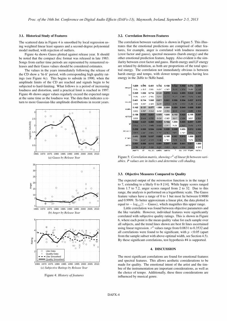
3.1. Historical Study of Features
The scattered data in Figure 4 is smoothed by local regression us-ing weighted linear least squares and a second-degree polynomialmodel method, with rejection of outliers.
Figure 4a shows Gauss plotted against release year. It shouldbe noted that the compact disc format was released in late 1983.Songs from earlier time periods are represented by remastered re-leases and their Gauss values should be considered estimates.
The values in the years immediately following the release ofthe CD show a ‘hi-fi’ period, with corresponding high quality rat-ings (see Figure 4c). This begins to subside in 1990, when theamplitude limits of the CD are reached and signals begin to besubjected to hard-limiting. What follows is a period of increasingloudness and distortion, until a practical limit is reached in 1997.Figure 4b shows anger values regularly exceed the expected rangeat the same time as the loudness war. The data then indicates a re-turn to more Gaussian-like amplitude distributions in recent years.
Like DataQuality DataLike SmoothedQuality Smoothed
(c) Subjective Ratings by Release Year
Figure 4: History of features
3.2. Correlation Between Features
The correlation between variables is shown in Figure 5. This illus-trates that the emotional predictions are comprised of other fea-tures, for example, anger is correlated with loudness measures(crest factor and gauss), spectral measures (harsh energy) and theother emotional prediction feature, happy. Also evident is the sim-ilarity between crest factor and gauss. Harsh energy and LF energyare related by definition, as both are proportions of the total spec-tral energy. The correlation not immediately obvious is betweenharsh energy and tempo, with slower tempo samples having lessenergy in the 2kHz to 5kHz band.
Figure 5: Correlation matrix, showing r2 of linear fit between vari-ables. P values are in italics and determine cell-shading.
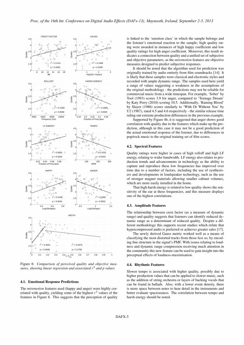
3.3. Objective Measures Compared to Quality
The expected output of the miremotion function is in the range 1to 7, extending to a likely 0 to 8 [14]. While happy scores rangedfrom 1.7 to 7.2, anger scores ranged from 2 to 32. Due to thisrange, the analysis is performed on a logarithmic scale. The Gaussfeature values have a range of 0 to 1 but most lie between 0.9000and 0.9999. To better approximate a linear plot, the data plotted isequal to − log10(1− Gauss), which magnifies this upper range.
Little correlation was found between objective parameters andthe like variable. However, individual features were significantlycorrelated with subjective quality ratings. This is shown in Figure6, where each point is the mean quality value for each sample overall subjects, and the trend lines shown are best fit lines ascertainedusing linear regression. r2 values range from 0.0831 to 0.3532 andall correlations were found to be significant, with p <0.05 (apartfrom the sample subset with above-optimal width, see Section 4.5).By these significant correlations, test hypothesis #4 is supported.
4. DISCUSSION
The most significant correlations are found for emotional featuresand spectral features. This allows aesthetic considerations to bemade for quality. The emotional intent of the artist and the tim-bre of the instrumentation are important considerations, as well asthe choice of tempo. Additionally, these three considerations areinfluenced by musical genre.
DAFX-4
Proc. of the 16th Int. Conference on Digital Audio Effects (DAFx-13), Maynooth, Ireland, September 2-5, 2013
Proc. of the 16th Int. Conference on Digital Audio Effects (DAFx-13), Maynooth, Ireland, September 2-6, 2013
8 10 12 14 16 182
2.5
3
3.5
4
4.5CREST FACTOR
dB
Qua
lity
r2 = 0.1211
p = 0.0092
1 2 32
2.5
3
3.5
4
4.5GAUSS
−log10(1−Gauss)
Qua
lity
r2 = 0.1484
p = 0.0290
4000 6000 8000 100002
2.5
3
3.5
4
4.5ROLLOFF
Frequency (Hz)
Qua
lity
r2 = 0.1350
p = 0.0058
0.15 0.2 0.25 0.3 0.352
2.5
3
3.5
4
4.5HARSH ENERGY
Fraction of Freq.Spec
Qua
lity
r2 = 0.1885
p = 0.0009
0.02 0.04 0.06 0.082
2.5
3
3.5
4
4.5LF ENERGY
Fraction of Freq.Spec
Qua
lity
r2 = 0.0831
p = 0.0328
100 150 2002
2.5
3
3.5
4
4.5TEMPO
BPM
Qua
lity
r2 = 0.1519
p = 0.0033
0.4 0.6 0.82
2.5
3
3.5
4
4.5HAPPY
Log10(Happy)
Qua
lity
r2 = 0.2108
p = 0.0004
0.5 1 1.52
2.5
3
3.5
4
4.5ANGER
Log10(Anger)
Qua
lity
r2 = 0.2382
p = 0.0002
0 0.1 0.2 0.3 0.4 0.5 0.6 0.7 0.8 0.9 12
2.5
3
3.5
4
4.5WIDTH
1−SLR
Qua
lity
r2 = 0.3532
p = 0.0045
r2 = 0.0370
p = 0.2759
Figure 6: Comparison of perceived quality and objective mea-sures, showing linear regression and associated r2 and p values
4.1. Emotional Response Predictions
The miremotion features used (happy and anger) were highly cor-related with quality, yielding some of the highest r2 values of thefeatures in Figure 6. This suggests that the perception of quality
is linked to the ‘emotion class’ in which the sample belongs andthe listener’s emotional reaction to the sample; high quality rat-ing were awarded in instances of high happy coefficient and lowquality ratings for high anger coefficient. Moreover, this result in-dicates a connection between quality and a unified set of subjectiveand objective parameters, as the miremotion features are objectivemeasures designed to predict subjective responses.
It should be noted that the algorithm used for prediction wasoriginally trained by audio entirely from film soundtracks [14]. Itis likely that these samples were classical and electronic styles andrecorded with ample dynamic range. The samples used here yielda range of values suggesting a weakness in the assumptions ofthe original methodology - the predictions may not be reliable forcommercial music from a wide timespan. For example, ‘Sober’ byTool (1993) scores 3.9 for anger, compared to ‘Teenage Dream’by Katy Perry (2010) scoring 10.5. Additionally, ‘Raining Blood’by Slayer (1986) scores similarly to ‘With Or Without You’ byU2 (1987), rated 4.5 and 4.6 respectively - the similar release timeruling out extreme production differences in the previous example.
Supported by Figure 4b, it is suggested that anger shows goodcorrelation with quality due to the features which make up the pre-diction, although in this case it may not be a good prediction ofthe actual emotional response of the listener, due to differences inpop/rock music to the original training set of film scores.
4.2. Spectral Features
Quality ratings were higher in cases of high rolloff and high LFenergy, relating to wider bandwidth. LF energy also relates to pro-duction trends and advancements in technology as the ability tocapture and reproduce these low frequencies has improved overtime due to a number of factors, including the use of synthesis-ers and developments in loudspeaker technology, such as the useof stronger magnet materials allowing smaller cabinet volumes,which are more easily installed in the home.
That high harsh energy is related to low quality shows the sen-sitivity of the ear at these frequencies, and this measure displaysone of the highest correlations.
4.3. Amplitude Features
The relationship between crest factor (as a measure of dynamicrange) and quality suggests that listeners can identify reduced dy-namic range as a determinant of reduced quality. Despite a dif-ferent methodology this supports recent studies which refute thathypercompressed audio is preferred or achieves greater sales [17].
The newly derived Gauss metric worked well as a means ofclassifying the most distorted tracks from those less so, by encod-ing fine structure in the signal’s PMF. With issues relating to loud-ness and dynamic range compression receiving much attention inthe community this new feature can be used to gain insight into theperceptual effects of loudness-maximisation.
4.4. Rhythmic Features
Slower tempo is associated with higher quality, possibly due tohigher production values that can be applied to slower music, suchas the addition of string orchestra or layers of backing vocals thatcan be found in ballads. Also, with a lower event density, thereis more space between notes to hear detail in the instruments andbetter evaluate spaciousness. The correlation between tempo andharsh energy should be noted.
DAFX-5
Proc. of the 16th Int. Conference on Digital Audio Effects (DAFx-13), Maynooth, Ireland, September 2-5, 2013
Proc. of the 16th Int. Conference on Digital Audio Effects (DAFx-13), Maynooth, Ireland, September 2-6, 2013
4.5. Spatial Features
While one linear model was not appropriate for width, an optimalvalue is found close to 0.17, where quality ratings reach a peak.This precise value was likely influenced by headphone playback,where sensitivity to width is enhanced. Due to this relationship,the width plot in Figure 6 shows two linear fits, with the datasetdivided into values above and below 0.17.
The data indicates that there is an increase in perceived qual-ity in going from monaural presentation to an ideal stereo width.However, wider-still samples saw no significant change in quality.For the reference of the reader, the samples used that measuredclosest to this optimal width are ‘Sledgehammer’ by Peter Gabriel(1986), ‘Superstition’ by Stevie Wonder (1972) and ‘Firestarter’by Prodigy (1996).
The optimal width was narrower than the mean width (0.25).This may be due to recent attempts in popular music production toproduce wider mixes, where this modern width may be presentingas lower-quality due to coincidence with modern dynamic rangereduction.
5. CONCLUSIONS AND FURTHER WORK
Correlations between objective measures of digital audio signalsand subjective measures of audio quality have been found for theopen-ended case of commercial music productions. Dynamics,distortions, tempo, spectral features and emotional predictions haveshown correlation with perceived audio quality.
A new objective signal parameter is proposed to unify crestfactor, clipping and other features of the audio PMF. This featureworks better than crest factor alone for identifying quality, andan analysis of how the feature varies with release year providesan insight into production trends and the evolution of the much-discussed loudness war. Some further work is needed to improveperformance, identify a more robust feature or to test the use of thehistogram itself as a feature vector.
Due to the correlations between objective measures and quality-perception it is anticipated that quality scores can be predicted bymeans of the extracted signal parameters. A number of possibleimplementations are being explored at the time of writing.
With only a relatively small test panel, the results are indica-tive rather than conclusive. Additional subjective testing wouldbe required to increase confidence in the findings. While con-cepts have been proven a greater number of audio samples andsubjects would be needed for future development. Such a listen-ing test would be well-suited to a mass-participation experiment,conducted on-line. The robustness of feature based quality predic-tions would benefit from this larger dataset, towards the goal ofautomatic quality-evaluation and subsequent enhancement.
6. REFERENCES
[1] ITU-R BS.1534-1, “Method for the subjective assessment ofintermediate quality levels of coding systems,” Tech. Rep.,International Telecommunication Union, Geneva, Switzer-land, Jan. 2003.
[2] ITU-T P.800, “Methods for objective and subjective assess-ment of quality,” Tech. Rep., International Telecommunica-tions Union, 1996.
[3] Amandine Pras, Rachel Zimmerman, Daniel Levitin, andCatherine Guastavino, “Subjective evaluation of mp3 com-pression for different musical genres,” in Audio EngineeringSociety Convention 127, 10 2009.
[4] Floyd E. Toole, “Loudspeaker measurements and their rela-tionship to listener preferences: Part 1,” J. Audio Eng. Soc,vol. 34, no. 4, pp. 227–235, 1986.
[5] Lorenz Rychner, “Featured review: Neu-mann KH 120 A Active Studio Monitor,”http://www.recordingmag.com/productreviews/2012/12/59.html,Accessed feb 1, 2013, 2012.
[6] Edmund Gurney, The Power of Sound, Cambridge Univer-sity Press, 2011, originally 1880.
[7] W. Hoeg, L. Christensen, and R. Walker, “Subjective assess-ment of audio quality - the means and methods within theebu,” EBU Technical Review, pp. 40–50, Winter 1997.
[8] Richard Repp, “Recording quality ratings by music profes-sionals,” in Proc. Intl. Computer Music Conf., New Orleans,USA, Nov. 6-11, 2006, pp. 468–474.
[9] Raimund Schatz, Sebastian Egger, and Kathrin Masuch,“The impact of test duration on user fatigue and reliabilityof subjective quality ratings,” J. Audio Eng. Soc, vol. 60, no.1/2, pp. 63–73, 2012.
[10] ITU-R BS.1116-1, “Methods for the subjective assessmentof small impairments in audio systems including multichan-nel sound systems,” Tech. Rep., International Telecommuni-cations Union, Vol. 1, pp. 1–11, 1997.
[11] Brian R. Glasberg and Brian C. J. Moore, “A model of loud-ness applicable to time-varying sounds,” J. Audio Eng. Soc,vol. 50, no. 5, pp. 331–342, 2002.
[12] Olivier Lartillot and Petri Toiviainen, “A matlab toolbox formusical feature extraction from audio,” in Proc. Digital Au-dio Effects (DAFx-07), Bordeaux, France, Sept. 10-15, 2007,pp. 237–244.
[13] George Tzanetakis and Perry R. Cook, “Musical genre clas-sification of audio signals,” IEEE Transactions on Speechand Audio Processing, vol. 10, no. 5, pp. 293–302, 2002.
[14] Tuomas Eerola, Olivier Lartillot, and Petri Toiviainen, “Pre-diction of multidimensional emotional ratings in music fromaudio using multivariate regression models,” in InternationalConference on Music Information Retrieval, Kobe, Japan,Oct. 26-30, 2009, pp. 621–626.
[15] Earl Vickers, “The loudness war: Background, speculation,and recommendations,” in Audio Engineering Society Con-vention 129, 11 2010.
[16] David Pensado, “Into The Lair #47 - Creat-ing Loud Tracks with EQ and Compression,”http://www.pensadosplace.tv/2012/09/18/into-the-lair-47-creating-loud-tracks-w-eq-and-compression/, accessedApril 4, 2013, September 2012.
[17] N.B.H. Croghan, K.H. Arehart, and J.M. Kates, “Qualityand loudness judgments for music subjected to compressionlimiting.,” J Acoust Soc Am, vol. 132, no. 2, pp. 1177–88,2012.
[18] Steven Fenton, Bruno Fazenda, and Jonathan Wakefield,“Objective measurement of music quality using inter-bandrelationship analysis,” in Audio Engineering Society Con-vention 130, 5 2011.
DAFX-6
Proc. of the 16th Int. Conference on Digital Audio Effects (DAFx-13), Maynooth, Ireland, September 2-5, 2013


![Acoustic Transparency and the Changing Soundscapeof ... · Spatial and Location Based Audio [63,101,12,62,89,85,68, 21] to Mediated Reality and Augmented Perception [99,24, 107,104,100,111].](https://static.documents.pub/doc/80x56/600b10a3e96a184e9d2b5210/acoustic-transparency-and-the-changing-soundscapeof-spatial-and-location-based.jpg)
![Perception & evaluation of audio quality in music …usir.salford.ac.uk/id/eprint/30255/1/04.dafx2013...oration in quality is measured [3]. Such descriptions would not strictly apply](https://static.documents.pub/doc/80x56/5e55f982a1f93c11d46dace8/perception-evaluation-of-audio-quality-in-music-usir-oration-in-quality.jpg)


