Perception & Thresholds of Nonlinear Distortion Using ... · The report investigates the audibility...

Section of Acoustics

Institute of Electronic Systems

Aalborg University

Perception & Thresholds of Nonlinear Distortion using Complex

Signals

Group 1061:Eric Mario de SantisSimon HeninSubmitted: June 7th 2007

Department of Electronic SystemsAalborg University

Section of Acoustics

THEME:Acoustics

SUBJECT:Investigation of thresholds of nonlinear distor-tion using improved metrics

TITLE:Perception & Thresholds of Nonlinear Distor-tion using Complex Signals

PROJECT PERIOD:

1. February 2007 -7. June 2007

GROUP:1061

GROUP MEMBERS:Eric Mario de SantisSimon Henin

SUPERVISOR:Per Rubak

NUMBER OF DUPLICATES: 5.

NUMBER OF PAGES IN REPORT: 65.

NUMBER OF PAGES IN APPENDIX: 17.

TOTAL NUMBER OF PAGES: 82.

Characterizing the perceptual effects ofnonlinear distortion by means of conventionalmetrics such as Total Harmonic Distortionand Intermodulation Distortion has proven tobe rather ineffectual. Conventional metricshave also proven unable to characterize theperception of nonlinear distortion in complexsignals, and thresholds for the perceptionof nonlinear distortion have been limited tosimple sinusoidal stimuli.

The use of improved metrics based on psy-choacoustic principles is studied from theperspective of determining the threshold ofperception of nonlinear distortion in complexsignals. The Distortion Score (DS) andRnonlin metrics are implemented and investi-gated by means of a verification experiment tostudy their correlation to subjective perceptionof nonlinear distortion. Once verified, themetrics are used to determine the thresholdof nonlinear distortion by means of anotherlistening experiment.

Nonlinear distortion thresholds for four typesof nonlinear devices are obtained using classi-cal and jazz music samples. The thresholds forclipping distortion are found to be much lowerthan second or third order distortion systems.The clipping distortion types are also nearlyindependent on the music type. For the sec-ond and third order distortion systems, the ob-tained thresholds are dependent on the charac-teristics of the music sample.

PREFACE

This report is written by Group 1061 at the Section of Acoustics at Aalborg University (AAU) and com-pleted during the spring semester of 2007. The report provides documentation pertaining to the group’sMaster’s thesis. The report investigates the audibility ofnonlinear distortion and threshold estimatesobtained using new nonlinear distortion metrics. The report itself is addressed to the staff and studentsat the Section of Acoustics at AAU and to anyone who has an interest in the perception of nonlineardistortion.

The report is divided into six chapters which include an introduction, problem analysis, implementationof the new nonlinear distortion metrics, design and analysis and experiment 1, design and analysis ofexperiment 2 and a final chapter containing both a discussionand conclusion. Graphs, measurementreports and other analysis not directly related to the report are included in the appendix.

A CD is provided along with the report containing:

• MATLAB code for listening test interfaces and selected simulations

• MATLAB code for the implemented nonlinear distortion metrics.

• Audio samples.

• The report in PDF format.

Eric Mario de Santis Simon Henin

CONTENTS

Preface 3

1 Introduction 1

1.1 Background . . . . . . . . . . . . . . . . . . . . . . . . . . . . . . . . . . . . . .. . . 1

1.2 Problem Statement . . . . . . . . . . . . . . . . . . . . . . . . . . . . . . . .. . . . . 2

2 Problem Analysis 3

2.1 Nonlinear Systems and Distortion . . . . . . . . . . . . . . . . . . .. . . . . . . . . . 3

2.2 Modeling Nonlinear Systems . . . . . . . . . . . . . . . . . . . . . . . .. . . . . . . . 6

2.3 Psychoacoustics of Distortion Perception . . . . . . . . . . .. . . . . . . . . . . . . . 8

2.4 Conventional Distortion Metrics . . . . . . . . . . . . . . . . . . .. . . . . . . . . . . 16

2.5 Multitone Test Stimulus . . . . . . . . . . . . . . . . . . . . . . . . . . .. . . . . . . . 19

2.6 Alternate Distortion Metrics . . . . . . . . . . . . . . . . . . . . . .. . . . . . . . . . 20

2.7 Methods of Threshold Estimation . . . . . . . . . . . . . . . . . . . .. . . . . . . . . 23

2.8 Summary . . . . . . . . . . . . . . . . . . . . . . . . . . . . . . . . . . . . . . . . .. 25

3 Implementation of Metrics 27

3.1 Implementation of the DS Metric . . . . . . . . . . . . . . . . . . . . .. . . . . . . . . 27

3.2 Implementation of The Rnonlin Metric . . . . . . . . . . . . . . . . . . . . . . . . . . . 30

3.3 Implementation of The THD & IMD Metrics . . . . . . . . . . . . . . .. . . . . . . . 35

3.4 Summary . . . . . . . . . . . . . . . . . . . . . . . . . . . . . . . . . . . . . . . . .. 36

4 Experiment 1: Verification of Metrics 37

4.1 Listening Evaluation to Determine Subjective Ratings of Nonlinear Distortion Systems . 37

4.2 Analysis of Results . . . . . . . . . . . . . . . . . . . . . . . . . . . . . . .. . . . . . 42

4.3 Verification of DS Metric . . . . . . . . . . . . . . . . . . . . . . . . . . .. . . . . . . 43

i

CONTENTS

4.4 Verification of Rnonlin Metric . . . . . . . . . . . . . . . . . . . . . . . . . . . . . . . . 43

4.5 Comparison with THD & IMD Metrics . . . . . . . . . . . . . . . . . . . .. . . . . . 44

4.6 Discussion of Results . . . . . . . . . . . . . . . . . . . . . . . . . . . . .. . . . . . . 47

4.7 Summary . . . . . . . . . . . . . . . . . . . . . . . . . . . . . . . . . . . . . . . . .. 47

5 Experiment 2: Determination of Nonlinear Distortion Thresholds 49

5.1 Thresholds of Nonlinear Distortion . . . . . . . . . . . . . . . . .. . . . . . . . . . . . 49

5.2 Test Implementation . . . . . . . . . . . . . . . . . . . . . . . . . . . . . .. . . . . . 51

5.3 Results from the Threshold Experiments . . . . . . . . . . . . . .. . . . . . . . . . . . 53

5.4 Discussion of Results . . . . . . . . . . . . . . . . . . . . . . . . . . . . .. . . . . . . 57

5.5 Summary . . . . . . . . . . . . . . . . . . . . . . . . . . . . . . . . . . . . . . . . .. 58

6 Discussion & Conclusions 61

A Measurement Reports 66

A.1 Harmonic and Intermodulation Distortion Products of Reproduction Chain . . . . . . . . 66

A.2 Headphone Impulse Response Measurement . . . . . . . . . . . . .. . . . . . . . . . . 69

B Loudness Normalization of Stimuli Using Loudness Model DIN 45631 (ISO 532B) 73

B.1 Zwicker’s Loudness Model . . . . . . . . . . . . . . . . . . . . . . . . . .. . . . . . . 73

C Rnonlin Curve Fitting 76

D Listening Experiments 79

D.1 Description of Listening Test Setup For Experiments 1 and 2 . . . . . . . . . . . . . . . 79

D.2 Instruction Sheet for Subjects . . . . . . . . . . . . . . . . . . . . .. . . . . . . . . . . 81

ii

CHAPTER 1

I NTRODUCTION

1.1 Background

The inadequacy of traditional nonlinear distortion metrics and the audio industry’s never ending pursuitof perfect sound reproduction has motivated research dedicated to the development of an appropriatemetric describing the human perception of nonlinear distortion. Conventional methods of nonlinear dis-tortion measurement only partly correlate with the perceived quality of reproduced sound. The task ofproviding a metric of nonlinear distortion is not a simple one. Such a metric must take many parametersinto account. These parameters would include the dependence of distortion detectability on the temporalcharacteristics and the frequency content of the signals used in listening evaluations, and the correlationbetween the physical effects causing nonlinear distortionand their corresponding detectability [3].

The conventional methods of measuring nonlinear distortion are based on the measurement of distortionproducts excited by a sinusoid or two or more sinusoids. These metrics are commonly known as TotalHarmonic Distortion (THD) and intermodulation distortion(IMD). They are typically expressed as aratio between the distortion by- products to the total system output [10]. There are many problems withthese metrics and to list them all is pointless as their main flaw is that these metrics are not at all cor-related with subjective ratings of nonlinear distortion. That is, they do not describe how we as humansperceive nonlinear distortion and to what extent we perceive nonlinear distortion.

A metric is a typically a single value parameter that facilitates the quantification of the characteristics ofa particular system. For instance, sound pressure can be a metric in the context of human sound percep-tion or temperature can be a metric for human perception of heat. The audio industry has the need fora proper metric relating to the human sound perception of nonlinear distortion. Building amplifiers orloudspeakers with distortion products far below audibility is unnecessary and expensive. Many investi-gations by many researchers often suggest different thresholds of distortion audibility [3]. However, aproper metric which is correlated with subjective ratings of distortion can be used to properly quantifyin some way the point where a listener can or cannot hear nonlinear distortion. The main theme of thisthesis is the utilization of the new nonlinear distortion metrics proposed by Moore et. al. [25][26] tofind this point, or threshold of nonlinear distortion audibility. These metrics, DS and Rnonlin , have beenfound to be highly correlated with subjective ratings of nonlinearly distorted speech and music signalsfor a variety of distortion types.

1

CHAPTER 1. INTRODUCTION

1.2 Problem Statement

Proper metrics which are well correlated with subject ratings of nonlinear distortion have been madeavailable as outlined in [25][26]. Obtaining a threshold interms of these metrics would offer the audioindustry assistance in the development of high quality products. Such thresholds of nonlinear distortioncould improve the manner in which manufacturers prove the quality of their products and reduce costsby ensuring that those systems do not have distortion products which are far below audibility.

Project Goal

The goal of this project is to obtain threshold estimates using the new nonlinear distortion metrics, DS andRnonlin . These estimates will be found for different types of music and for different nonlinear distortiontypes. The following list details the main goals which this thesis will evaluate:

1. The influence of the music sample on the obtained threshold.

2. The influence of the distortion type on the obtained threshold.

Project Scope

In order to arrive at the nonlinear distortion threshold using the new metrics the following steps must betaken:

1. Understanding and Implementation of the nonlinear distortion metrics DS and Rnonlin .

2. Verification of the new metrics’ correlation with subjectratings of nonlinear distortion.

3. Design of a listening experiment to obtain the nonlinear distortion thresholds.

4. Analysis of the obtained thresholds in relation to the project goal.

2

CHAPTER 2

PROBLEM ANALYSIS

This section presents the fundamental theories behind nonlinear systems as well as important psychoa-coustical principles relating to the perception of nonlinear distortion. Finally, an overview of conven-tional metrics used in evaluating nonlinear distortion is presented along with alternate distortion metricsthat aim at developing a metric that relates nonlinear distortion to subjective perception.

2.1 Nonlinear Systems and Distortion

Signal distortion resulting from acoustical transducers and transmission channels can be classified asbeing either linear or nonlinear. Linear distortion affects the amplitudes and phases of the frequencycomponents present in a complex signal. This type of distortion can be compensated for by applyinglinear filtering methods. As an example, an equalizer can be used to compensate for the undesirablefrequency response caused by a certain loudspeaker. In contrast to linear distortion, nonlinear distortioninjects frequency components that were not present in the original signal. The effects of nonlinear dis-tortion are difficult and sometimes impossible to compensate for [25].

A linear system is described as having the following mathematical properties:

1. Additivity: f(x + y) = f(x) + f(y)

2. Homogeneity:f(ax) = a ∗ f(x)

Together, these two properties of linear systems are referred to as the principle of superposition. A sys-tem is said to be nonlinear if its input and output characteristics are not linearly related mathematically.That is, the system does not obey the principle of superposition.

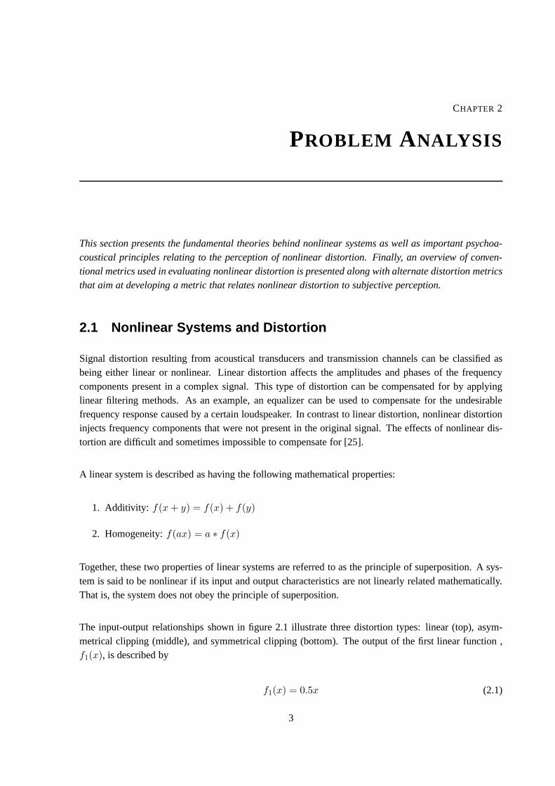
The input-output relationships shown in figure 2.1 illustrate three distortion types: linear (top), asym-metrical clipping (middle), and symmetrical clipping (bottom). The output of the first linear function ,f1(x), is described by

f1(x) = 0.5x (2.1)

3

CHAPTER 2. PROBLEM ANALYSIS

wherex is the input signal.

The function,f2(x), describing the asymmetrical clipping is:

f2(x) =

{

x if x < 0.5

0.5 if x ≥ 0.5(2.2)

This system is referred to as asymmetrical nonlinear distortion as the clipping is only applied to half ofthe waveform (positive cycle).

The function,f3(x), describing the symmetrical nonlinear distortion is defined by:

f3(x) =

x if 0.5 < x < 0.5

0.5 if x ≥ 0.5

−0.5 if x ≤ −0.5

(2.3)

As the clipping is applied to both positive and negative cycles, the distortion is referred to as being sym-metrical.

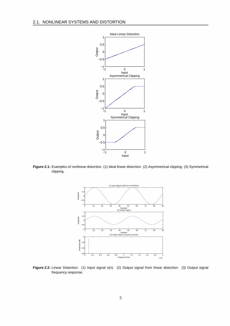
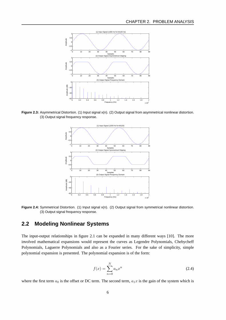
A discrete time input signal,x(n) = sin(2π1000nT ), is plotted at the top of figures 2.2, 2.3 and 2.4with a sampling frequency offs = 44100 Hz. The output signal resulting from the signal,x(n), passingthrough the distortion systems described above is plotted in both the time and frequency domain.

The output signal from the linear distortion system shown infigure 2.2 has the same phase as the originalsignal differing only in amplitude. The change in amplitudeis also evident in the frequency domain asshown in the bottom graph of figure 2.2. As expected, the frequency spectrum from this linear systemcontains the same frequency component as the original signal. The original frequency is known as thefundamental.

The output signal plotted in figure 2.3 has the same amplitudeas the original signal on the negative cyclebut has been clipped to 0.5 on the positive cycle. This type ofdistortion injects both even and odd orderharmonics throught the spectrum decreasing in magnitude with increasing frequency. An even harmonicoccurs at even multiples of the fundamental frequency,2f, 4f, 6f, 8f..... Odd order harmonics occur atodd multipes of the fundamental frequency,1f, 3f, 5f, 7f..... The presence of frequency componentsnot existing in the original input signal characterizes thesystems nonlinear behavior.

The output signal from shown in figure 2.4 has been clipped to 0.5 on both the positive and negativecycles. Overdriven solid state devices exhibit this type ofnonlinear distortion. In contrast with the asym-metrical distortion, the added frequency components occurat only odd multiples of the input frequency.

4

2.1. NONLINEAR SYSTEMS AND DISTORTION

−1 0 1−1

−0.5

0

0.5

1Ideal Linear Distortion

Input

Out

put

−1 0 1−1

−0.5

0

0.5

1Asymmetrical Clipping

Input

Out

put

−1 0 1−1

−0.5

0

0.5

1Symmetrical Clipping

Input

Out

put

Figure 2.1: Examples of nonlinear distortion. (1) Ideal linear distortion. (2) Asymmetrical clipping. (3) Symmetricalclipping.

0 10 20 30 40 50 60 70 80 90−1

−0.5

0

0.5

1(1) Input Signal (1000 Hz fs=44100Hz)

Samples

Am

plitu

de

0 10 20 30 40 50 60 70 80 90−1

−0.5

0

0.5

1

Samples

Am

plitu

de

(2) Output Signal

0 0.2 0.4 0.6 0.8 1 1.2 1.4 1.6 1.8 2

x 104

−60

−40

−20

0

Frequency (Hz)

Am

plitu

de (

dB)

(3) Output Signal Frequency Domain

Figure 2.2: Linear Distortion. (1) Input signal x(n). (2) Output signal from linear distortion. (3) Output signalfrequency response.

5


0 10 20 30 40 50 60 70 80 90−1

−0.5

0

0.5

1

Samples

Am

plitu

de

(2) Output Signal Asymmetrical Clipping

0 10 20 30 40 50 60 70 80 90−1

−0.5

0

0.5

1(1) Input Signal (1000 Hz fs=44100 Hz)

Am

plitu

de

Samples

0 0.2 0.4 0.6 0.8 1 1.2 1.4 1.6 1.8 2

x 104

−60

−40

−20

0

Frequency (Hz)

Am

plitu

de (

dB)


Figure 2.3: Asymmetrical Distortion. (1) Input signal x(n). (2) Output signal from asymmetrical nonlinear distortion.(3) Output signal frequency response.

0 10 20 30 40 50 60 70 80 90−1

−0.5

0

0.5

1

Samples

Am

plitu

de

(1) Input Signal (1000 Hz fs=44100)

0 10 20 30 40 50 60 70 80 90−1

−0.5

0

0.5

1

Samples

Am

plitu

de

(2) Output Signal Symmetrical Clipping

0 0.2 0.4 0.6 0.8 1 1.2 1.4 1.6 1.8 2

x 104

−60

−40

−20

0

Frequency (Hz)

Am

plitu

de (

dB)


Figure 2.4: Symmetrical Distortion. (1) Input signal x(n). (2) Output signal from symmetrical nonlinear distortion.(3) Output signal frequency response.

2.2 Modeling Nonlinear Systems

The input-output relationships in figure 2.1 can be expandedin many different ways [10]. The moreinvolved mathematical expansions would represent the curves as Legendre Polynomials, ChebycheffPolynomials, Laguerre Polynomials and also as a Fourier series. For the sake of simplicity, simplepolynomial expansion is presented. The polynomial expansion is of the form:

f(x) =

N∑

n=0

anxn (2.4)

where the first terma0 is the offset or DC term. The second term,a1x is the gain of the system which is

6

2.2. MODELING NONLINEAR SYSTEMS

also the linear portion of the expansion. The third term,a2x2, is the second order (quadratic) nonlinearity.

The third term,a3x3 is the third order (cubic) nonlinearity. Even order polynomials will contribute only

even order harmonics and odd order polynomials odd harmonics. For example, the polynomial,x5 willhave harmonic components at multiples of1, 3, 5 times the fundamental frequency. For a pure tone, theoutput of the nonlinear system will contain only harmonic components of the input frequency. However,the output resulting from a more complex tone being passed through the system will not only containthe harmonic components of the frequencies present in the tone, but also sum and difference componentsbetween those frequencies. These sum of difference components are known as intermodulation products.

To illustrate mathematically how the output of a nonlinear system produces both harmonic and intermod-ulation products, a general equation for cubic nonlinearity is considered in equation 2.5. An input signalconsisting of two frequencies is shown in equation 2.6.

f(x) = a1x + a3x3 (2.5)

x = bsin(ω1t) + csin(ω2t) (2.6)

f(x) =

a1

(

bsin(ω1t) + csin(ω2t))

+

a3

(

(3b3

4 + 3bc2

2 )sin(ω1t) + (3c3

4 + 3b2c2 )sin(ω2t)

)

−

a34

(

b3sin(3ω1t) + c3sin(3ω2t))

−

3a3b2c4

(

sin((ω2 − 2ω1)t) + sin((2ω1 + ω2)t))

−

3a3bc2

4

(

sin((ω1 − 2ω2)t) + sin((2ω2 + ω1)t)

(2.7)

The output signal shown in the above equation can be described as follows: the first line in equation 2.7represents the linear term which is simply a gain determinedby the coefficienta1. The second line inequation 2.7 is the first order distortion product and the third line in equation 2.7 represents the third or-der harmonic distortion products. The fourth and fifth linesshow the intermodulation distortion productsresulting from the interaction between the two input frequencies.

To illustrate the use of these expansions, polynomial expansion was applied to the nonlinear distortionsystems described in the above section. The frequency components present in the output signals fromboth the asymmetrical and symmetrical nonlinear distortion systems contain high order harmonic com-ponents spanning up to 18th harmonic. Intuitively, a high order expansion will be able to model thenonlinear system more accurately.

The MATLAB function, polyfit, was used to generate an nth order polynomial based on two data vec-tors. These data vectors contain both the input and output signals from each system. The function fitsthe datap(x) to y in the least squared sense. The function returns an nth orderpolynomial according theto the equation below.

7


p(x) = p(1)xn + p(2)xn−1...pnx + pn+1 (2.8)

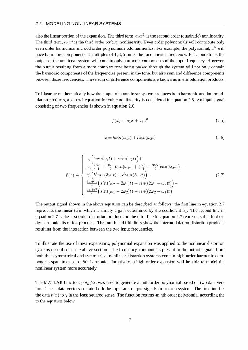
Both nonlinear distortion system were modeled with two polynomials of different order. The first ex-pansion order was selected as a third order polynomial as this would be the minimum order possible torepresent both odd and even order harmonics. The higher order polynomial expansion was of 7th order.The input sequence was the same 1000 Hz discrete time signal used in the previous section.

Figure 2.5 plots the time and frequency domain output from the 3rd and 7th order polynomial expansionsof the asymmetrical nonlinear distortion. The clipping in the 7th order model is more defined than that ofthe lower order representation. The 7th order model has morefrequency components than the 3rd ordermodel and in both cases even and odd order harmonics are present. The amplitude of the representedharmonic components is nearly equal to the equivalent harmonic components in the actual frequencyresponse of the asymmetrical system in figure 2.3.

0 10 20 30 40 50 60 70 80 90−1

0

1

Samples

Am

plitu

de

0 0.2 0.4 0.6 0.8 1 1.2 1.4 1.6 1.8 2

x 104

−60

−40

−20

0

Frequency (Hz)

Am

plitu

de (

dB)

0 10 20 30 40 50 60 70 80 90−1

0

1

Samples

Am

plitu

de

0 0.2 0.4 0.6 0.8 1 1.2 1.4 1.6 1.8 2

x 104

−60

−40

−20

0

Frequency (Hz)

Am

plitu

de (

dB)

Figure 2.5: Polynomial expansion of asymmetrical type distortion. (Top: Output signal from 3rd order model. Sec-ond from Top: Frequency spectrum of output signal. Third from top: Output signal from 7th order model.Bottom: Frequency spectrum of output signal.)

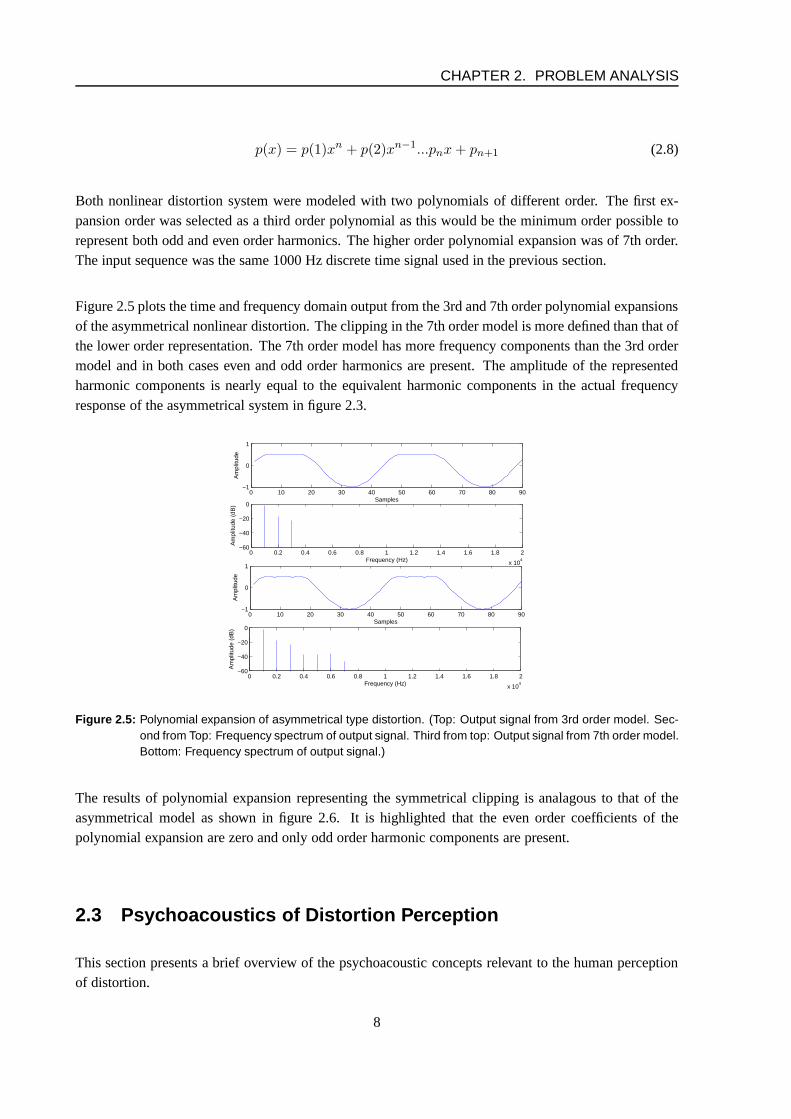
The results of polynomial expansion representing the symmetrical clipping is analagous to that of theasymmetrical model as shown in figure 2.6. It is highlighted that the even order coefficients of thepolynomial expansion are zero and only odd order harmonic components are present.

2.3 Psychoacoustics of Distortion Perception

This section presents a brief overview of the psychoacoustic concepts relevant to the human perceptionof distortion.

8

2.3. PSYCHOACOUSTICS OF DISTORTION PERCEPTION

0 10 20 30 40 50 60 70 80 90−1

0

1

Samples

Am

plitu

de

0 0.2 0.4 0.6 0.8 1 1.2 1.4 1.6 1.8 2

x 104

−60

−40

−20

0

Am

plitu

de (

dB)

Frequency (Hz)

0 10 20 30 40 50 60 70 80 90−1

0

1

Samples

Am

plitu

de

0 0.2 0.4 0.6 0.8 1 1.2 1.4 1.6 1.8 2

x 104

−60

−40

−20

0

Frequency (Hz)

Am

plitu

de (

dB)

Figure 2.6: Polynomial expansion of symmetrical type distortion. (Top: Output signal from 3rd order model. Secondfrom Top: Frequency spectrum of output signal. Third from top: Output signal from 7th order model.Bottom: Frequency spectrum of output signal.)

Hearing Thresholds

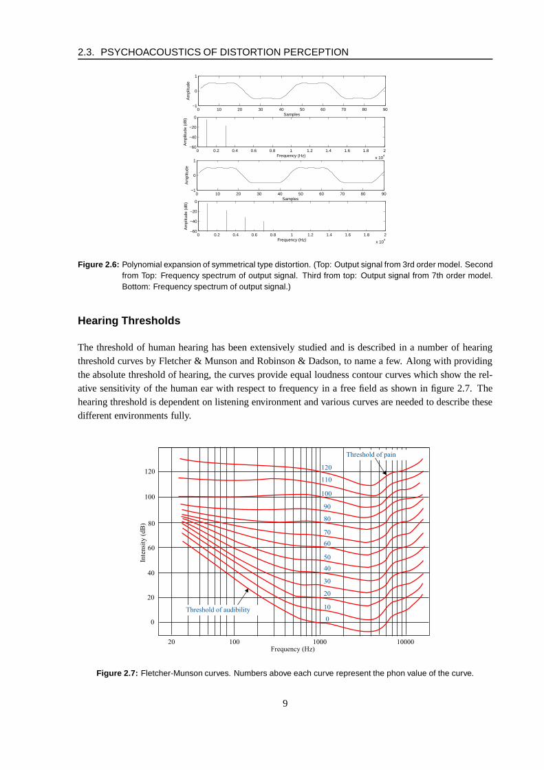
The threshold of human hearing has been extensively studiedand is described in a number of hearingthreshold curves by Fletcher & Munson and Robinson & Dadson,to name a few. Along with providingthe absolute threshold of hearing, the curves provide equalloudness contour curves which show the rel-ative sensitivity of the human ear with respect to frequencyin a free field as shown in figure 2.7. Thehearing threshold is dependent on listening environment and various curves are needed to describe thesedifferent environments fully.

Figure 2.7: Fletcher-Munson curves. Numbers above each curve represent the phon value of the curve.

9


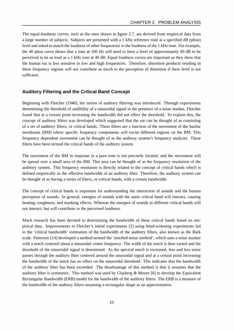
The equal-loudness curves, such as the ones shown in figure 2.7, are derived from empirical data froma large number of subjects. Subjects are presented with a 1 kHz reference tone at a specified dB (phon)level and asked to match the loudness of other frequencies tothe loudness of the 1 kHz tone. For example,the 40 phon curve shows that a tone at 100 Hz will need to have a level of approximately 60 dB to beperceived to be as loud as a 1 kHz tone at 40 dB. Equal loudness curves are important as they show thatthe human ear is less sensitive to low and high frequencies. Therefore, distortion products residing inthese frequency regions will not contribute as much to the perception of distortion if there level is notsufficient.

Auditory Filtering and the Critical Band Concept

Beginning with Fletcher (1940), the notion of auditory filtering was introduced. Through experimentsdetermining the threshold of audibility of a sinusoidal signal in the presence of a noise masker, Fletcherfound that at a certain point increasing the bandwidth did not effect the threshold. To explain this, theconcept of auditory filters was developed which suggested that the ear can be thought of as consistingof a set of auditory filters, or critical bands. These filters are a function of the movement of the basilarmembrane (BM) where specific frequency components will excite different regions on the BM. Thisfrequency dependent movement can be thought of as the auditory system’s frequency analyzer. Thesefilters have been termed the critical bands of the auditory system.

The movement of the BM in response to a pure tone is not precisely located, and the movement willbe spread over a small area of the BM. This area can be thought of as the frequency resolution of theauditory system. This frequency resolution is directly related to the concept of critical bands which isdefined empirically as the effective bandwidth of an auditory filter. Therefore, the auditory system canbe thought of as having a series of filters, or critical bands,with a certain bandwidth.

The concept of critical bands is important for understanding the interaction of sounds and the humanperception of sounds. In general, energies of sounds with the same critical band will interact, causingbeating, roughness, and masking effects. Whereas the energies of sounds in different critical bands willnot interact, but will contribute to the perceived loudness.

Much research has been devoted to determining the bandwidthof these critical bands based on em-pirical data. Improvements to Fletcher’s initial experiments [5] using band-widening experiments ledto the ’critical bandwidth’ estimation of the bandwidth of the auditory filters, also known as the Barkscale. Patterson [14] developed a method termed the ’notched-noise method’, which uses a noise maskerwith a notch centered about a sinusoidal center frequency. The width of the notch is then varied and thethreshold of the sinusoidal signal is determined. As the spectral notch is increased, less and less noisepasses through the auditory filter centered around the sinusoidal signal and at a certain point increasingthe bandwidth of the notch has no effect on the sinusoidal threshold. This indicates that the bandwidthof the auditory filter has been exceeded. The disadvantage ofthis method is that it assumes that theauditory filter is symmetric. This method was used by Glasberg & Moore [6] to develop the EquivalentRectangular Bandwidth (ERB) model for the bandwidth of the auditory filters. The ERB is a measure ofthe bandwidth of the auditory filters assuming a rectangularshape as an approximation.

10


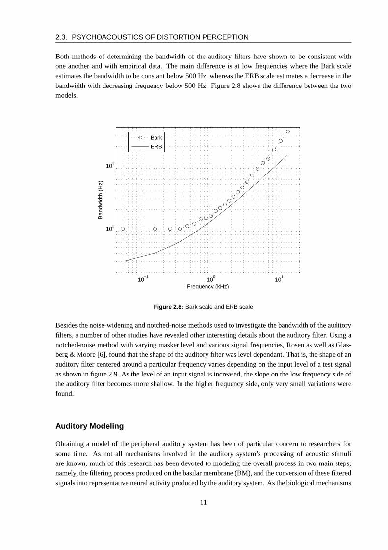
Both methods of determining the bandwidth of the auditory filters have shown to be consistent withone another and with empirical data. The main difference is at low frequencies where the Bark scaleestimates the bandwidth to be constant below 500 Hz, whereasthe ERB scale estimates a decrease in thebandwidth with decreasing frequency below 500 Hz. Figure 2.8 shows the difference between the twomodels.

10−1

100

101

102

103

Frequency (kHz)

Ban

dwid

th (

Hz)

Bark

ERB

Figure 2.8: Bark scale and ERB scale

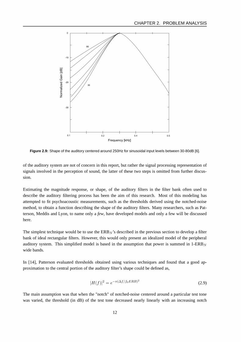
Besides the noise-widening and notched-noise methods usedto investigate the bandwidth of the auditoryfilters, a number of other studies have revealed other interesting details about the auditory filter. Using anotched-noise method with varying masker level and varioussignal frequencies, Rosen as well as Glas-berg & Moore [6], found that the shape of the auditory filter was level dependant. That is, the shape of anauditory filter centered around a particular frequency varies depending on the input level of a test signalas shown in figure 2.9. As the level of an input signal is increased, the slope on the low frequency side ofthe auditory filter becomes more shallow. In the higher frequency side, only very small variations werefound.

Auditory Modeling

Obtaining a model of the peripheral auditory system has beenof particular concern to researchers forsome time. As not all mechanisms involved in the auditory system’s processing of acoustic stimuliare known, much of this research has been devoted to modelingthe overall process in two main steps;namely, the filtering process produced on the basilar membrane (BM), and the conversion of these filteredsignals into representative neural activity produced by the auditory system. As the biological mechanisms

11


Figure 2.9: Shape of the auditory centered around 250Hz for sinusoidal input levels between 30-80dB [6].

of the auditory system are not of concern in this report, but rather the signal processing representation ofsignals involved in the perception of sound, the latter of these two steps is omitted from further discus-sion.

Estimating the magnitude response, or shape, of the auditory filters in the filter bank often used todescribe the auditory filtering process has been the aim of this research. Most of this modeling hasattempted to fit psychoacoustic measurements, such as the thresholds derived using the notched-noisemethod, to obtain a function describing the shape of the auditory filters. Many researchers, such as Pat-terson, Meddis and Lyon, to name only afew, have developed models and only a few will be discussedhere.

The simplest technique would be to use the ERBN ’s described in the previous section to develop a filterbank of ideal rectangular filters. However, this would only present an idealized model of the peripheralauditory system. This simplified model is based in the assumption that power is summed in 1-ERBN

wide bands.

In [14], Patterson evaluated thresholds obtained using various techniques and found that a good ap-proximation to the central portion of the auditory filter’s shape could be defined as,

|H(f)|2 = e−π(∆f/f0ERB)2 (2.9)

The main assumption was that when the "notch" of notched-noise centered around a particular test tonewas varied, the threshold (in dB) of the test tone decreased nearly linearly with an increasing notch

12


width. This indicated that the shape of the auditory could bedescribed approximately by an exponentialfunction.

Patterson’s initial model shown in equation 2.9 was furtherrevised into the concept of the "rounded-exponential", orroex, function [20]. Theroex model assumed that the filter shape could be representedby a pair of back-to-back exponential functions. The simplest form of one of these exponential functionsis described by,

W (g) = (1 + pg)e−pg (2.10)

whereg is the distance from the filter center frequency,fc, to the evaluation point,f , normalized withrespect to the signal frequency such thatg = |f − fc|/f0 [19], andp is a function parameter used totune the bandwidth and the slopes of the skirts. Equation 2.10 is termed theroex(p) function as its onlyparameter isp and is used primarily to model the passband of the auditory filter. The level-dependentasymmetry of the auditory filter could be implemented by using different parameter values on the lowerand upper halves of the model (roex(pl; pu)).

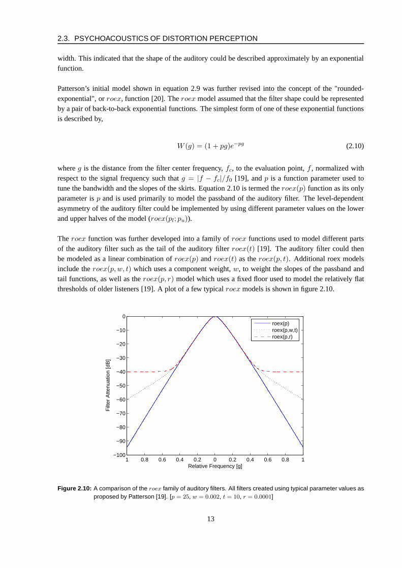
Theroex function was further developed into a family ofroex functions used to model different partsof the auditory filter such as the tail of the auditory filterroex(t) [19]. The auditory filter could thenbe modeled as a linear combination ofroex(p) androex(t) as theroex(p, t). Additional roex modelsinclude theroex(p,w, t) which uses a component weight,w, to weight the slopes of the passband andtail functions, as well as theroex(p, r) model which uses a fixed floor used to model the relatively flatthresholds of older listeners [19]. A plot of a few typicalroex models is shown in figure 2.10.

1 0.8 0.6 0.4 0.2 0 0.2 0.4 0.6 0.8 1−100

−90

−80

−70

−60

−50

−40

−30

−20

−10

0

Relative Frequency [g]

Filt

er A

ttenu

atio

n [d

B]

roex(p)roex(p,w,t)roex(p,r)

Figure 2.10: A comparison of the roex family of auditory filters. All filters created using typical parameter values asproposed by Patterson [19]. [p = 25, w = 0.002, t = 10, r = 0.0001]

13


Although theroex models were found to fit measured data very well, the obvious limitation is that theyonly offer a frequency domain model. Roex models are used solely to filter stimuli in the frequency do-main by specifying the relative attenuation of the modeled filters. Methods implementing an inverse-fftto create the time domain representations failed to capturecorrectly the phase response of the auditoryfilters and were not defined for discontinuous models, such astheroex(p,w, t) [29].

Boer [1] first proposed the gammatone function for modeling the shape of the impulse response functionof the auditory system as estimated by a reverse correlation("revcor") function of neural firing times incats [15]. The shape of the magnitude response was found to bevery similar to that of theroex modelat moderate sound levels, and so it was developed into a time-domain model of the auditory filter byPatterson [17, 16, 15]. The gammatone filter is described as,

g(t) = αtn−1e−2nbtcos(2nfct + φ), for t > 0 (2.11)

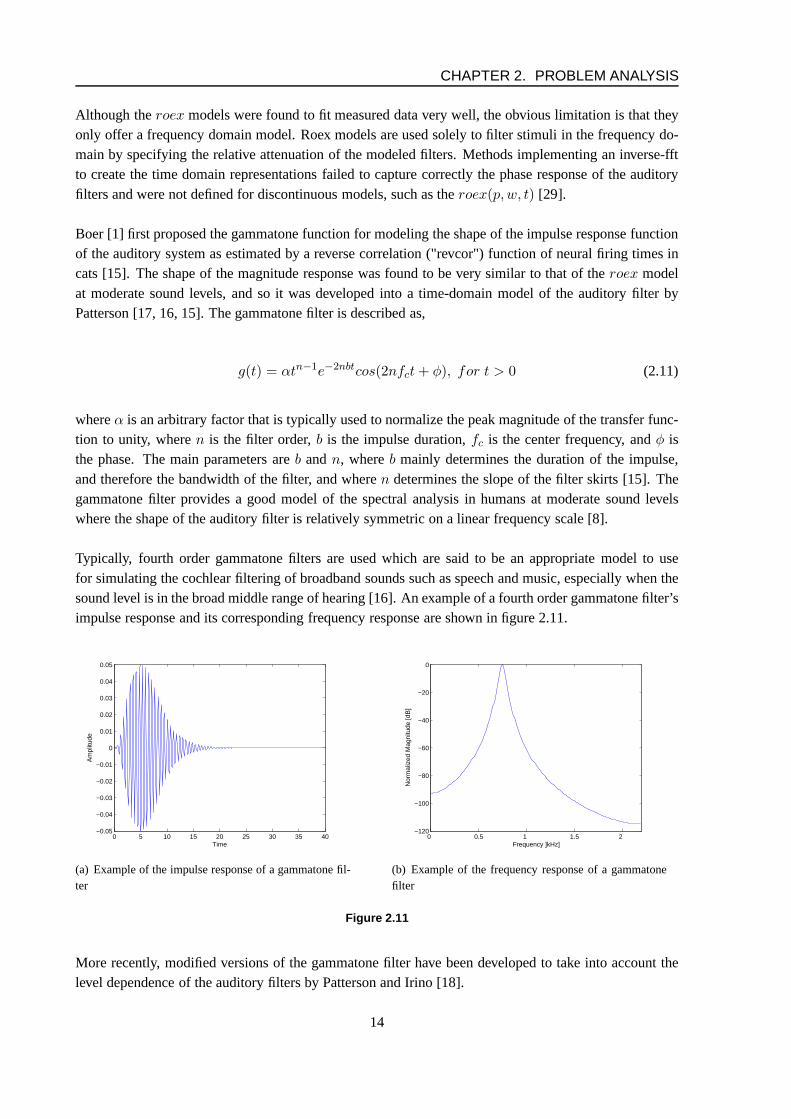
whereα is an arbitrary factor that is typically used to normalize the peak magnitude of the transfer func-tion to unity, wheren is the filter order,b is the impulse duration,fc is the center frequency, andφ isthe phase. The main parameters areb andn, whereb mainly determines the duration of the impulse,and therefore the bandwidth of the filter, and wheren determines the slope of the filter skirts [15]. Thegammatone filter provides a good model of the spectral analysis in humans at moderate sound levelswhere the shape of the auditory filter is relatively symmetric on a linear frequency scale [8].

Typically, fourth order gammatone filters are used which aresaid to be an appropriate model to usefor simulating the cochlear filtering of broadband sounds such as speech and music, especially when thesound level is in the broad middle range of hearing [16]. An example of a fourth order gammatone filter’simpulse response and its corresponding frequency responseare shown in figure 2.11.

0 5 10 15 20 25 30 35 40−0.05

−0.04

−0.03

−0.02

−0.01

0

0.01

0.02

0.03

0.04

0.05

Time

Am

plitu

de

(a) Example of the impulse response of a gammatone fil-ter

0 0.5 1 1.5 2 −120

−100

−80

−60

−40

−20

0

Frequency ]kHz]

Nor

mal

ized

Mag

nitu

de [d

B]

(b) Example of the frequency response of a gammatonefilter

Figure 2.11

More recently, modified versions of the gammatone filter havebeen developed to take into account thelevel dependence of the auditory filters by Patterson and Irino [18].

14


Auditory Masking

The concept of auditory masking refers to the psychoacoustic phenomenon of one stimulus, audible inisolation, being rendered inaudible in the presence of a masking stimulus. A typical example would bethe masking of speech by background noise such as road traffic.

In general, masking depends on loudness where a loud sound will mask a soft sound. Masking alsodepends on frequency. In general, sounds mask frequencies higher than the frequency of the sound itselfmore than frequencies below the masker. Additionally, sounds within a critical band mask each othermore than those more than a critical bandwidth apart. Complex tones are more difficult to mask thanpure tones.

The primary mechanisms thought to be involved in the processof masking are swamping and suppres-sion. Swamping suggests that the neural activity evoked by the masker may render the neural activityproduced by the target stimulus undetectable. Suppressionsuggests that the masker stimulus may sup-press the neural response of the target stimulus.

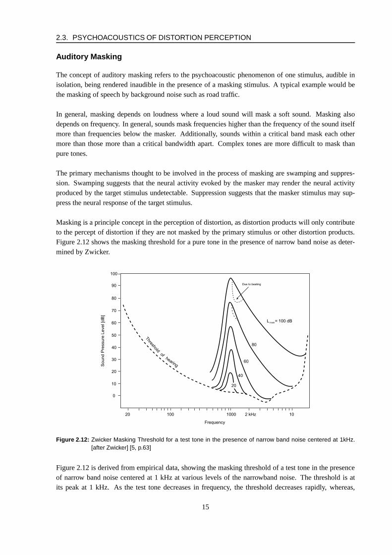
Masking is a principle concept in the perception of distortion, as distortion products will only contributeto the percept of distortion if they are not masked by the primary stimulus or other distortion products.Figure 2.12 shows the masking threshold for a pure tone in thepresence of narrow band noise as deter-mined by Zwicker.

Figure 2.12: Zwicker Masking Threshold for a test tone in the presence of narrow band noise centered at 1kHz.[after Zwicker] [5, p.63]

Figure 2.12 is derived from empirical data, showing the masking threshold of a test tone in the presenceof narrow band noise centered at 1 kHz at various levels of thenarrowband noise. The threshold is atits peak at 1 kHz. As the test tone decreases in frequency, thethreshold decreases rapidly, whereas,

15


when the test tone frequency is increased past 1 kHz, the threshold decreases more slowly. From figure2.12, two things should be noted; first, masking predominately effects higher frequencies rather thanlower frequencies [5]. Second, that the masking effect increases nonlinearly with an increase in themasker level. As an example, an increase from 60 dB to 80 dB in the noise level of the masker will pro-duce a 30 dB increase in the masking threshold at 3 kHz, as seenin the Zwicker masking threshold curve.

In the case of harmonic distortion, this masking threshold could have an effect on different harmonicswith relation to their distance to the fundamental. As an example, given a nonlinear system produc-ing 2nd and 3rd harmonics with equal amplitudes, the 2nd harmonics would be masked more than the3rd harmonic. This principle can also be applied to higher order harmonics with the idea being thathigher order harmonics will be perceived more than lower order harmonics and will therefore be moreperceptible.

Factors Effecting Distortion Perception

Of particular note in the psychoacoustics of distortion perception are frequency discrimination of distor-tion by-products as well as temporal effects of distortion perception.

It has been found that harmonic distortion below 400 Hz is harder to detect than harmonic distortionabove 400 Hz [12, 27]. This can be partially explained by the fact that the threshold of hearing increasesat low frequencies.

Additionally, temporal effects have an impact on the perception distortion due to the finite time reso-lution of the ear. In studies conducted by Moir [12], it was found that the "just detectable" distortiondecreased with increased presentation time. Specifically,it was found that for a 4ms tone burst distortedby clipping, the just detectable distortion reached approximately 10%, while increasing the presentationtime to 20ms reduced the just detectable distortion level to0.3% [12] .

2.4 Conventional Distortion Metrics

The classic distortion metric for harmonic distortion is known as total harmonic distortion (THD). TheTHD is defined as the ratio of the square of the root-mean-square (rms) values of the harmonics to thatof the fundamental. The THD can be expressed mathematicallyas:

%THD = 100

√

V 22 + V 2

3 + V 24 + ...V 2

n

VT(2.12)

whereVn is the rms value of each harmonic component andVT is the rms value of the fundamental.Typically, a high purity sine wave is used as an input to the nonlinear system to excite the harmonic com-ponents. A frequency analyzer can be used to measure the rms value of all the harmonic components andthe THD can be found using the above equation. This procedureis rather tedious and is it quite oftenquite difficult to measure harmonic distortion products with precision (especially since most solid-stateaudio devices have such low distortion).

16

2.4. CONVENTIONAL DISTORTION METRICS

The THD+N metric is often provided instead of the THD. This method is based on the same procedure asfor the THD, however, this parameter also includes any othernoise present in the system. The numeratorof the above ratio is determine by removing the fundamental from the output of the nonlinear device bymeans of a notch filter. The total rms voltage of this signal includes all the harmonic components plusany other noise. The denominator of the above equation is therms level of the entire signal including thefundamental, harmonics and additional noise. Removing thefundamental by subtracting the output ofthe nonlinear device by the input signal could also be performed instead of using a notch filter. However,many systems will provide some phase shifting and as a resultthe simple subtraction would not work asthe output and input fundamental would not be in phase.

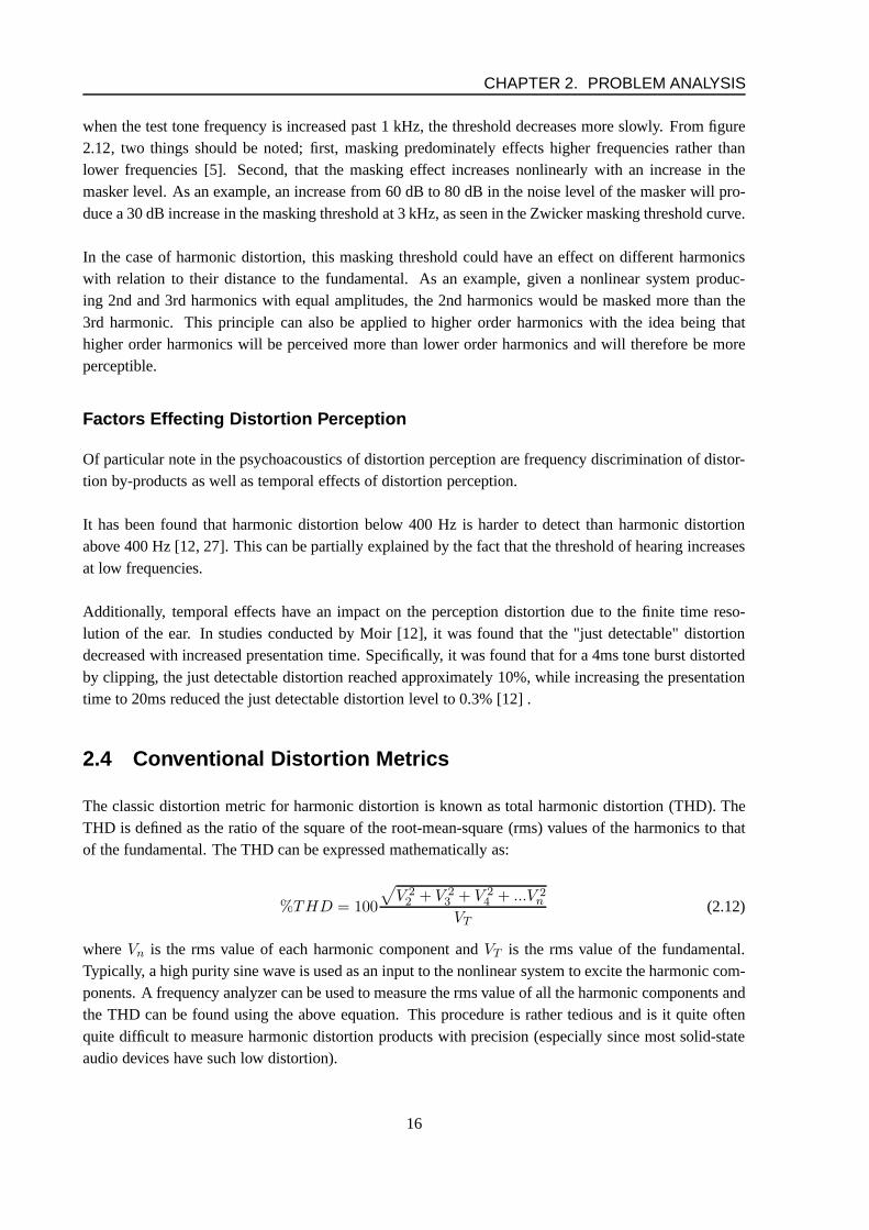
Using a pure tone input to a nonlinear device does not excite intermodulation products. A metric, inter-modulation distortion (IMD), quantifies distortion products not related harmonically to the fundamental.Two standard methods for measurement and evaluation of the IMD will be discussed. These standardsare the SMPTE test (Society of Motion Picture and TelevisionEngineers) and the CCIF. For the SMPTEIMD method two standard frequencies atfl=60 Hz andfh=7 kHz with a 4:1 amplitude difference (12dB)are mixed together for the input signal to the nonlinear system. The upper intermodulation componentsare spaced at multiples of the lower frequency component as shown in Figure 2.13(a). The rms sumbetween the distortion products is evaluated and expressedas a ratio against the rms value of the upperfrequency component (7 kHz).

In contrast to the SMPTE method, the CCIF (difference frequency distortion) method uses two frequen-cies of equal amplitude with a 1 kHz difference. The distortion products can be found in Figure 2.13(b).The rms sum between the distortion products is evaluated andexpressed as a ratio against the rms valueof the input signal. Even order distortion produces the lower difference frequency components and theodd order the higher difference frequency components closer to the input signals . Most applications ofthis test only measure the lower even order distortion products [2]. Typical input frequencies are often14 kHz and 15 kHz, which effectively eliminate any harmonic contribution to the measurement.

(a) SMPTE Test for IMD (b) CCIF Test for IMD

Figure 2.13: Comparison of the SMPTE and CCIF methods for calculating the IMD metric.

Problems with THD Metric

As described above, the THD provides a measure for the total contribution of harmonic distortion by-products in a resultant output signal. As a metric, it provides a good indication of the amount of harmonic

17


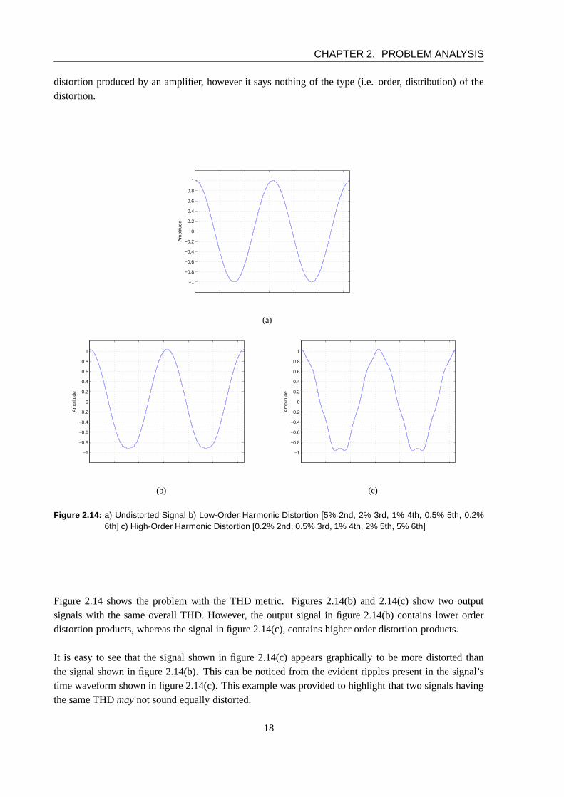
distortion produced by an amplifier, however it says nothingof the type (i.e. order, distribution) of thedistortion.

−1

−0.8

−0.6

−0.4

−0.2

0

0.2

0.4

0.6

0.8

1A

mpl

itude

(a)

−1

−0.8

−0.6

−0.4

−0.2

0

0.2

0.4

0.6

0.8

1

Am

plitu

de

(b)

−1

−0.8

−0.6

−0.4

−0.2

0

0.2

0.4

0.6

0.8

1

Am

plitu

de

(c)

Figure 2.14: a) Undistorted Signal b) Low-Order Harmonic Distortion [5% 2nd, 2% 3rd, 1% 4th, 0.5% 5th, 0.2%6th] c) High-Order Harmonic Distortion [0.2% 2nd, 0.5% 3rd, 1% 4th, 2% 5th, 5% 6th]

Figure 2.14 shows the problem with the THD metric. Figures 2.14(b) and 2.14(c) show two outputsignals with the same overall THD. However, the output signal in figure 2.14(b) contains lower orderdistortion products, whereas the signal in figure 2.14(c), contains higher order distortion products.

It is easy to see that the signal shown in figure 2.14(c) appears graphically to be more distorted thanthe signal shown in figure 2.14(b). This can be noticed from the evident ripples present in the signal’stime waveform shown in figure 2.14(c). This example was provided to highlight that two signals havingthe same THDmaynot sound equally distorted.

18

2.5. MULTITONE TEST STIMULUS

2.5 Multitone Test Stimulus

The inadequacy of the current metrics such as THD and IMD is primarily a result of the test signals usedin deriving the metrics. This consists of the use of single sinusoids or sweeping sinusoids in the case ofthe THD metric and a two tone signal in the case of the IMD metric. Although adequate in describing thespecific contribution of harmonic or intermodulation components in a distorted signal, the test signalsdo not provide an accurate picture of the distortion introduced in more realistic signals, such as musicsignals.

The THD and IMD metrics are based on the output of a nonlinear device to a single tone or two toneinput test signal. These test signals only excite either harmonic distortion products or intermodulationproducts. This fails to encapsulate the complete interaction of all distortion products making it difficultcorrelate these metrics with a subjective relevant quantity. By using a multitone stimulus, a more com-plete picture of the nonlinear distortion can be realized.

The concept of using a multitone test stimulus was introduced by Czerwinski et. al. [3, 4] as meansof capturing an increased amount of information as to the type and content of the distortion introducedby a nonlinear system. The multitone test stimulus can be described as,

x(t) =

N∑

i=1

Aisin(ωit + φi) (2.13)

whereωi andφi are the frequency and the starting phase of theith tone, respectively.

The frequency components of the multitone signal are logarithmically spaced in order to place the fun-damental tones into a non-harmonic relationship so as to avoid any distortion components being hiddenwithin the primary signal. For example, if a two component multitone signal has frequencies at 1 and 2kHz then second harmonic components could be produced at 2 and 4 kHz. The 2 kHz harmonic distortionproduct would interact with the 2 kHz component of the multitone signal. Additionally, the logarithmicspacing avoids periodicity of the resulting signal [3].

Determining the number and frequency distribution of the multitone components is primarily determinedby the application. Increasing the number of tones in the multitone signal makes the signal resemble anoise or musical signal more closely. However, increasing the number of tones also increases the crestfactor of the signal which is not desired. Minimization of the crest factor in the multitone signal is desir-able since it increases the dynamic range of measurement by decreasing signal peaks, increasing the rmslevel of the signal and increasing the signal-to-noise ratio [3]. The crest factor is defined as,

CF =|A|max

Arms(2.14)

In general, it is desired to have the smallest crest factor possible in the multitone signal in order to in-crease the dynamic range possible with the measurement. This is due to the fact that signal peaks thatare far above the overall rms level of a signal do not permit the dynamic range to be excited evenly sinceenergy in the signal is not equally spread. In order to achieve a proper balance of the crest factor, a trade-

19


off between the number, spacing, and starting phases of the multitone components must be configuredproperly based on the application.

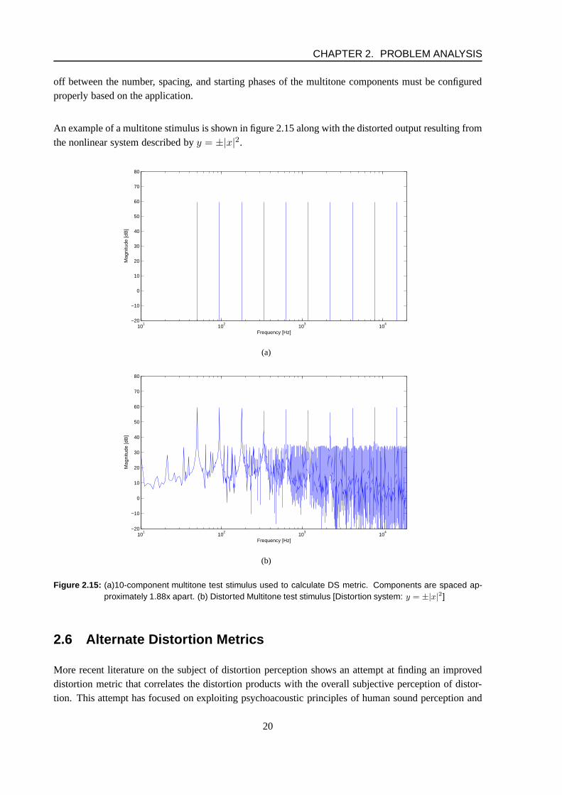
An example of a multitone stimulus is shown in figure 2.15 along with the distorted output resulting fromthe nonlinear system described byy = ±|x|2.

101

102

103

104

−20

−10

0

10

20

30

40

50

60

70

80

Frequency [Hz]

Mag

nitu

de [d

B]

(a)

101

102

103

104

−20

−10

0

10

20

30

40

50

60

70

80

Frequency [Hz]

Mag

nitu

de [d

B]

(b)

Figure 2.15: (a)10-component multitone test stimulus used to calculate DS metric. Components are spaced ap-proximately 1.88x apart. (b) Distorted Multitone test stimulus [Distortion system: y = ±|x|2]

2.6 Alternate Distortion Metrics

More recent literature on the subject of distortion perception shows an attempt at finding an improveddistortion metric that correlates the distortion productswith the overall subjective perception of distor-tion. This attempt has focused on exploiting psychoacoustic principles of human sound perception and

20

2.6. ALTERNATE DISTORTION METRICS

applying them to derive metrics that more accurately reflectthe effects of distortion and the perception ofthe distortion. Such metrics allow for more meaningful measurements that not only quantify the amountof nonlinear distortion, but also relate these quantities to a certain subjective perception. Three importantmetrics are the Gedlee metric proposed by Geddes & Lee [10, 9], the DS metric proposed by Moore et.al [25], and the Rnonlin metric proposed by Moore et. al [26].

GedLee Metric

The GedLee (Gm) metric was derived primarily based on the psychoacoustic properties of masking, asdescribed in Section 2.3. The authors proposed a metric to take into account two principle effects ofmasking. The first being that higher order harmonics are moreperceptible due to the tendency of lowerorder harmonics to be masked. The second, that nonlinear distortion products will be more audible atlow signal levels since the masking threshold at low signal levels is lower than at higher levels. (refer tofigure 2.12 on page 15, masking threshold) Additionally, theproposed metric is to be immune to offsetand gain characteristics of the output signal, since these effects are either linear contributions to the inputsignal or imperceptible.

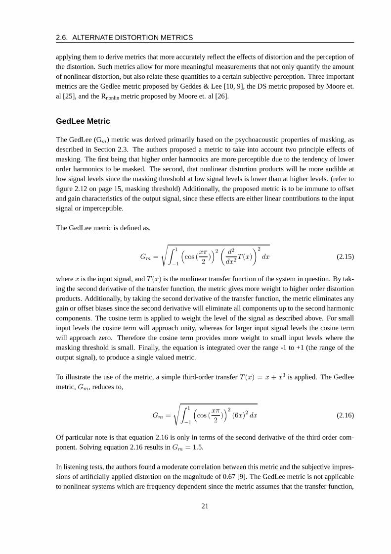
The GedLee metric is defined as,

Gm =

√

∫ 1

−1

(

cos (xπ

2))2(

d2

dx2T (x)

)2

dx (2.15)

wherex is the input signal, andT (x) is the nonlinear transfer function of the system in question. By tak-ing the second derivative of the transfer function, the metric gives more weight to higher order distortionproducts. Additionally, by taking the second derivative ofthe transfer function, the metric eliminates anygain or offset biases since the second derivative will eliminate all components up to the second harmoniccomponents. The cosine term is applied to weight the level ofthe signal as described above. For smallinput levels the cosine term will approach unity, whereas for larger input signal levels the cosine termwill approach zero. Therefore the cosine term provides moreweight to small input levels where themasking threshold is small. Finally, the equation is integrated over the range -1 to +1 (the range of theoutput signal), to produce a single valued metric.

To illustrate the use of the metric, a simple third-order transferT (x) = x + x3 is applied. The Gedleemetric,Gm, reduces to,

Gm =

√

∫ 1

−1

(

cos (xπ

2))2

(6x)2 dx (2.16)

Of particular note is that equation 2.16 is only in terms of the second derivative of the third order com-ponent. Solving equation 2.16 results inGm = 1.5.

In listening tests, the authors found a moderate correlation between this metric and the subjective impres-sions of artificially applied distortion on the magnitude of0.67 [9]. The GedLee metric is not applicableto nonlinear systems which are frequency dependent since the metric assumes that the transfer function,

21


T (x), is valid for all frequencies. The nonlinear distortion in real transducers often varies with fre-quency. As such, it was recommended in [26] that the GedLee metric be extended into frequency bandsand applying the metric separately in each band.

Distortion Score (DS) Metric

The Distortion Score (DS) is a more elaborate metric that attempts to take into account the psychoa-coustic process of auditory filtering in deriving the metric. As described in section 2.3, psychoacousticmodels for the human auditory system assume that energies within a critical band interact to producethe overall perception of the sound within that band, such asthe masking of a tone by narrowband noise[5]. The DS metric attempts to model the auditory system using the Equivalent Rectangular Bandwidths(ERBN ) developed by Moore [13]. The Difference Score relates to the difference between the overallspectrum produced by the input signal as compared to the overall spectrum produced by the output signalincluding its distortion products.

The steps involved in determining the value of DS of a given signal are crudely given as follows: First,an input signal is passed through a nonlinear system giving rise to an output signal. The input and outputsignals are time aligned so as to remove any time delays introduced by the nonlinear system. Next, theinput and output signals are analyzed in a series of 30ms frames. The 30 ms time frame is typicallychosen to ensure that the Discrete Fourier Transform (DFT) is performed over a stationary signal. TheDFT is performed over each frame, and the relative peaks of the output signal are normalized to the inputsignal to remove any offset or gain bias. This ensures that any linear distortion is removed from theoutput signal. The signal spectra are grouped into appropriate ERBN frequency bands so as to have arepresentation of the signal’s "frequency analysis" in theauditory system. The overall power of the inputand output signals in each band is then calculated and converted to decibels. Finally, the absolute valueof the difference in each band is then summed across all bandsresulting in the DS value.

According to the authors, this gives a’perceptually relevant measure of the difference spectrumbetweenthe input and the output’[26]. Using subjective ratings of distortion obtained for avariety of test stimuliand nonlinear distortion systems, the authors found the metric to be highly correlated with the subjec-tive perception of distortion perception with correlationvalues up to 0.97 for music and speech signals.However, more moderate values of correlation, 0.60-0.67, were found when distortion produced by realtransducers was used. The lower correlation of the DS metricwith subject ratings of real transducerswas pointed out in [26] to be a result of the crude modeling of the frequency analysis in the peripheralauditory system used in the DS metric’s algorithm.

Rnonlin Metric

The Rnonlin metric was developed as an extension of the DS metric developed by Moore et. al. in [25] asdescribed above. As the performance of the DS metric using real distortion produced by real transducerswas only moderate, the Rnonlin metric was proposed using a different approach to analyzingthe differ-ence between the input test signal and its distorted output.Instead of calculating a difference score basedon the input and output spectrum, a coherence analysis was performed by taking the cross-correlationbetween the input and distorted output waveforms. Additionally, the metric algorithm uses a more com-

22

2.7. METHODS OF THRESHOLD ESTIMATION

prehensive model of the frequency analysis performed in theperipheral auditory system including thefiltering produced by the outer and middle ear. Figure 3.2 shows a block diagram of the steps involvedin deriving the Rnonlin metric.

Similar to the DS metric, an input signal is passed through a nonlinear system resulting in a distortedoutput signal. Additionally, the input and output waveforms are time aligned to remove any unwanteddelays caused by the nonlinear system. Next, both waveformsare filtered to mimic the response of theouter and middle ear by 4097 FIR filters, as described by Glasberg and Moore [7]. Next, both waveformsare filtered by an array of 40 gammatone filters with a bandwidth of 1-ERBN . This filtering provides amore elaborate modeling of the auditory filtering mechanismas described by Patterson et. al. [17].

Next, the input and output signals are split into 30ms framesfor further processing. The maximumvalue of the normalized cross-correlation between the input and output signals, Xmax, is calculated. Foreach frame, the Xmax values are summed across all filters. Finally, the Xmax values are averaged overall the frames resulting in the single valued metric, Rnonlin .

2.7 Methods of Threshold Estimation

The principle aim of this project relates to the applicationof the new nonlinear distortion metrics, DS andRnonlin , to nonlinear distortion thresholds. Obtaining a threshold implies increasing or decreasing someindependent variable to find the point at which the subjective response to an auditory event changes.Hearing thresholds, for instance, vary the sound pressure level of a pure tone signal to the point, orthreshold, where the subject can no longer hear the signal.

There are various methods available to experimenters to arrive at a given threshold. One such method,the method of constants, presents pre-determined samples with a varying parameter to a subject in ran-dom presentation order and the subject is asked to determinewhich samples are audible and which arenot with respect to the parameter in question. Once the test is finished, the distribution of positive andnegative responses is calculated and the threshold may be determined. While this method provides a wayto ensure an unbiased result, it requires a larger number samples and may take an excessive amount oftime if only the threshold is of interest [11].

Another method labeled the method of limits, presents a sample with a high probability of a positiveresponse to a subject. Based on the response of the subject, the subsequent sample presentation is ei-ther increased or decreased in level accordingly until the threshold is reached, indicated by a negativeresponse, or reversal. At this point the test is over and the threshold is determined as the reversal point.This may be done in either an ascending or descending fashion, where the threshold is approached fromeither below or above the threshold, respectively. While simple in its implementation, it provides nosafeguard against false-positives and may yield misleading results.

The simple up-down method is similar to the method of limits,however the test is not finished afterthe first reversal. The simple up-down procedure, within thecontext of distortion, would decrease the

23


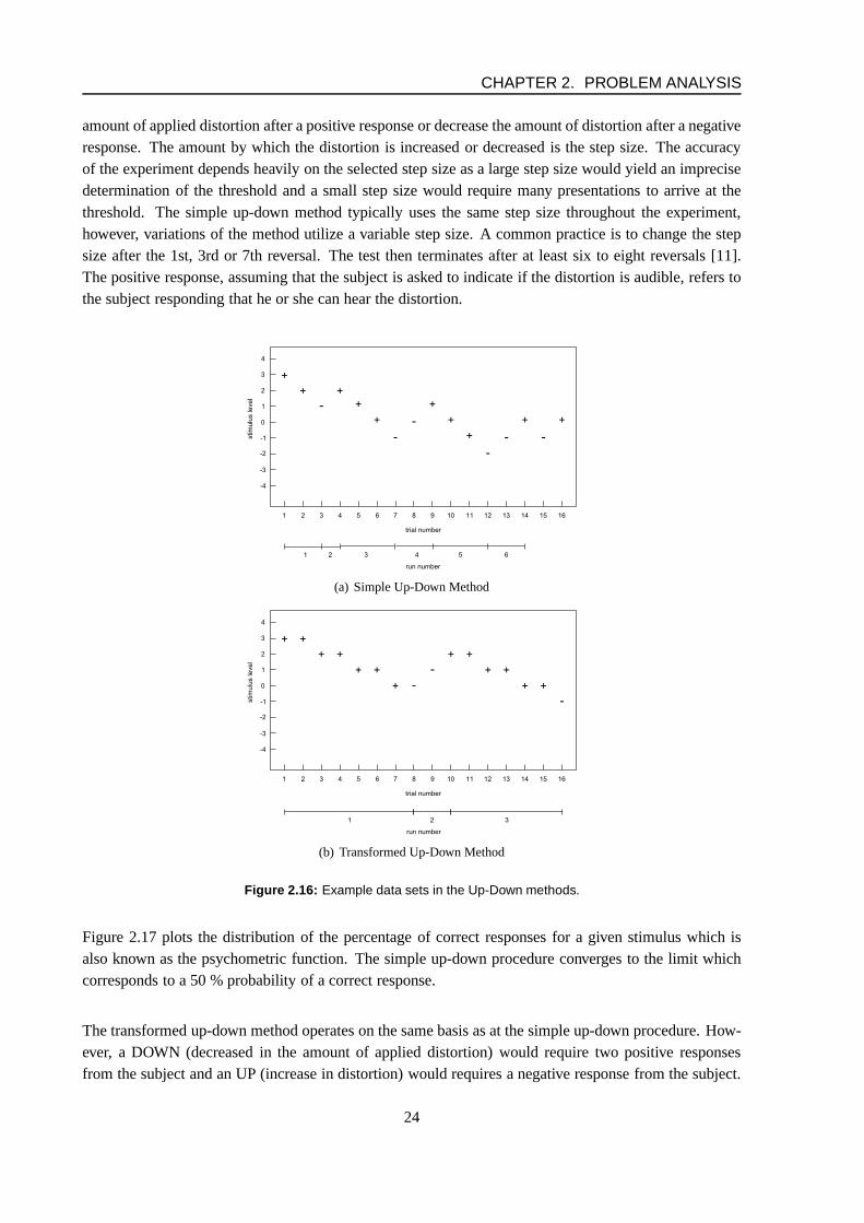
amount of applied distortion after a positive response or decrease the amount of distortion after a negativeresponse. The amount by which the distortion is increased ordecreased is the step size. The accuracyof the experiment depends heavily on the selected step size as a large step size would yield an imprecisedetermination of the threshold and a small step size would require many presentations to arrive at thethreshold. The simple up-down method typically uses the same step size throughout the experiment,however, variations of the method utilize a variable step size. A common practice is to change the stepsize after the 1st, 3rd or 7th reversal. The test then terminates after at least six to eight reversals [11].The positive response, assuming that the subject is asked toindicate if the distortion is audible, refers tothe subject responding that he or she can hear the distortion.

(a) Simple Up-Down Method

(b) Transformed Up-Down Method

Figure 2.16: Example data sets in the Up-Down methods.

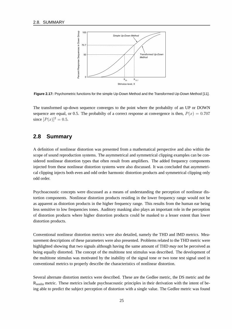
Figure 2.17 plots the distribution of the percentage of correct responses for a given stimulus which isalso known as the psychometric function. The simple up-downprocedure converges to the limit whichcorresponds to a 50 % probability of a correct response.

The transformed up-down method operates on the same basis asat the simple up-down procedure. How-ever, a DOWN (decreased in the amount of applied distortion)would require two positive responsesfrom the subject and an UP (increase in distortion) would requires a negative response from the subject.

24

2.8. SUMMARY

Figure 2.17: Psychometric functions for the simple Up-Down Method and the Transformed Up-Down Method [11].

The transformed up-down sequence converges to the point where the probabilty of an UP or DOWNsequence are equal, or 0.5. The probabilty of a correct response at convergence is then,P (x) = 0.707

since[P (x)]2 = 0.5.

2.8 Summary

A definition of nonlinear distortion was presented from a mathematical perspective and also within thescope of sound reproduction systems. The asymmetrical and symmetrical clipping examples can be con-sidered nonlinear distortion types that often result from amplifiers. The added frequency componentsinjected from these nonlinear distortion systems were alsodiscussed. It was concluded that asymmetri-cal clipping injects both even and odd order harmonic distortion products and symmetrical clipping onlyodd order.

Psychoacoustic concepts were discussed as a means of understanding the perception of nonlinear dis-tortion components. Nonlinear distortion products residing in the lower frequency range would not beas apparent as distortion products in the higher frequency range. This results from the human ear beingless sensitive to low frequencies tones. Auditory masking also plays an important role in the perceptionof distortion products where higher distortion products could be masked to a lesser extent than lowerdistortion products.

Conventional nonlinear distortion metrics were also detailed, namely the THD and IMD metrics. Mea-surement descriptions of these parameters were also presented. Problems related to the THD metric werehighlighted showing that two signals although having the same amount of THDmaynot be perceived asbeing equally distorted. The concept of the multitone test stimulus was described. The development ofthe multitone stimulus was motivated by the inability of thesignal tone or two tone test signal used inconventional metrics to properly describe the characteristics of nonlinear distortion.

Several alternate distortion metrics were described. These are the Gedlee metric, the DS metric and theRnonlin metric. These metrics include psychoacoustic principles in their derivation with the intent of be-ing able to predict the subject perception of distortion with a single value. The Gedlee metric was found

25


to have only moderate correlation to subject ratings of distortion. The DS and Rnonlin metrics were foundto have quite high correlation with subjective ratings of distortion. For the purposes of the nonlinear dis-tortion thresholds, it is most necessary to have a highly correlated metric. As such, the Gedlee parameteris not considered for future implementation and analysis.

Experimental methods for obtaining a threshold within the scope of human experimental psychologywere detailed. These methods included the method of constants, the method of limits and the simple up-down method. Finally, the transformed up-down method was arrived at which improves the efficiencyand threshold estimation of the simple up-down procedure.

26

CHAPTER 3

I MPLEMENTATION OF M ETRICS

This chapter provides a detailed description of the DS and Rnonlin metrics. The algorithms for bothmetrics were implemented in MATLAB. The methods for calculating the the THD+N metric and the IMDmetric according to the CCIF standard are also presented. These metrics will be used in Chapter 4 toverify the correlation of these metrics to subjective ratings of distortion.

3.1 Implementation of the DS Metric

This section presents the implementation of the DS metric developed by Moore et. al. [25] The programwas developed in MATLAB and a block diagram of the metric is shown in figure 3.1.

Description of the DS Model

The underlying idea in deriving the DS metric is to find the difference between the input and outputspectrum of a signal after undergoing nonlinear distortion. Additionally, the metric aims at taking intoaccount the peripheral auditory filtering process in its derivation.

The steps involved in determining the value of DS of a given signal are as follows: First, an multi-tone input signal is passed through a nonlinear system giving rise to an output signal. The input andoutput signals are time aligned so as to remove any time delays introduced by the system. Next, the inputand output signals are analyzed in a series of 30ms frames. A 1323 point Discrete Fourier Transform(DFT) is performed over each frame,i, and the relative peaks of the output signal are scaled to theinputsignal to remove any offset or gain bias. The is accomplishedby finding the maximum value of the 1323frequency bins from both the output and input signals. The peak value of the output signal is then scaleddown to the peak value of the input signal. The signal spectraare then grouped into 40 non-overlappingERBN frequency bands covering the center frequencies from 50-19739 Hz. This provides a perceptuallyrelevant representation of the signal processed by the auditory system. The overall power of the inputand output signals in each band is calculated and converted to decibels. Finally, the absolute value of thedifference in each band is then summed across all bands, resulting in the DS metric.

27

CHAPTER 3. IMPLEMENTATION OF METRICS

Figure 3.1: Block Diagram for the calculation of the DS Metric.

Multitone Test Stimulus

As mentioned in Section 2.5, determining the number of tonesneeded for the multitone signal greatlydepends upon the application. In [25], Moore et. al. used subjective ratings of distortion to find the bestcorrelation between the number tones and relative phases inthe multitone signal to the ratings. Theyfound that a 10-component multitone stimulus with a spacingof approximately1.88f resulted in thegreatest correlation between DS and subjective rating.

Deriving the ERB Filter Bank

Using the notched noise method described in section 2.3, Moore & Glasberg [6], determined the Equiva-lent Rectangular Bandwidth (ERB) of the auditory filters. The mean values of the ERB’s measured using

28

3.1. IMPLEMENTATION OF THE DS METRIC

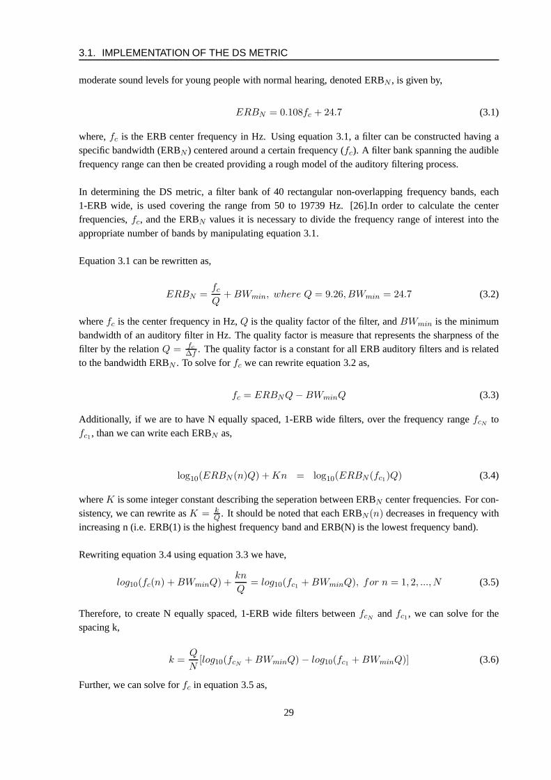
moderate sound levels for young people with normal hearing,denoted ERBN , is given by,

ERBN = 0.108fc + 24.7 (3.1)

where,fc is the ERB center frequency in Hz. Using equation 3.1, a filtercan be constructed having aspecific bandwidth (ERBN ) centered around a certain frequency (fc). A filter bank spanning the audiblefrequency range can then be created providing a rough model of the auditory filtering process.

In determining the DS metric, a filter bank of 40 rectangular non-overlapping frequency bands, each1-ERB wide, is used covering the range from 50 to 19739 Hz. [26].In order to calculate the centerfrequencies,fc, and the ERBN values it is necessary to divide the frequency range of interest into theappropriate number of bands by manipulating equation 3.1.

Equation 3.1 can be rewritten as,

ERBN =fc

Q+ BWmin, where Q = 9.26, BWmin = 24.7 (3.2)

wherefc is the center frequency in Hz,Q is the quality factor of the filter, andBWmin is the minimumbandwidth of an auditory filter in Hz. The quality factor is measure that represents the sharpness of thefilter by the relationQ = fc

∆f . The quality factor is a constant for all ERB auditory filtersand is relatedto the bandwidth ERBN . To solve forfc we can rewrite equation 3.2 as,

fc = ERBNQ − BWminQ (3.3)

Additionally, if we are to have N equally spaced, 1-ERB wide filters, over the frequency rangefcNto

fc1, than we can write each ERBN as,

log10(ERBN (n)Q) + Kn = log10(ERBN (fc1)Q) (3.4)

whereK is some integer constant describing the seperation betweenERBN center frequencies. For con-sistency, we can rewrite asK = k

Q . It should be noted that each ERBN(n) decreases in frequency withincreasing n (i.e. ERB(1) is the highest frequency band and ERB(N) is the lowest frequency band).

Rewriting equation 3.4 using equation 3.3 we have,

log10(fc(n) + BWminQ) +kn

Q= log10(fc1 + BWminQ), for n = 1, 2, ..., N (3.5)

Therefore, to create N equally spaced, 1-ERB wide filters betweenfcNandfc1, we can solve for the

spacing k,

k =Q

N[log10(fcN

+ BWminQ) − log10(fc1 + BWminQ)] (3.6)

Further, we can solve forfc in equation 3.5 as,

29


fc(n) =fc1 + BWminQ

10knQ

− BWminQ, for n = 1, 2, ..., N (3.7)

By insertingk from equation 3.6 into equation 3.7, we can solve forfc(n) as,

fc(n) =fc1 + BWminQ

10(Q

N[log10(fc1+BWminQ)−log10(fcN

+BWminQ)]

Q )n− BWminQ, for n = 1, 2, ..., N (3.8)

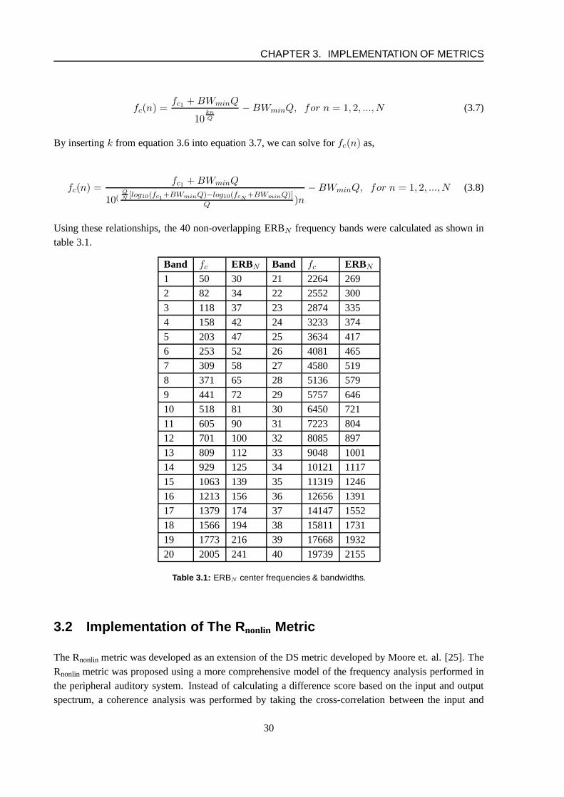
Using these relationships, the 40 non-overlapping ERBN frequency bands were calculated as shown intable 3.1.

Band fc ERBN Band fc ERBN

1 50 30 21 2264 269

2 82 34 22 2552 300

3 118 37 23 2874 335

4 158 42 24 3233 374

5 203 47 25 3634 417

6 253 52 26 4081 465

7 309 58 27 4580 519

8 371 65 28 5136 579

9 441 72 29 5757 646

10 518 81 30 6450 721

11 605 90 31 7223 804

12 701 100 32 8085 897

13 809 112 33 9048 1001

14 929 125 34 10121 1117

15 1063 139 35 11319 1246

16 1213 156 36 12656 1391

17 1379 174 37 14147 1552

18 1566 194 38 15811 1731

19 1773 216 39 17668 1932

20 2005 241 40 19739 2155

Table 3.1: ERBN center frequencies & bandwidths.

3.2 Implementation of The R nonlin Metric

The Rnonlin metric was developed as an extension of the DS metric developed by Moore et. al. [25]. TheRnonlin metric was proposed using a more comprehensive model of the frequency analysis performed inthe peripheral auditory system. Instead of calculating a difference score based on the input and outputspectrum, a coherence analysis was performed by taking the cross-correlation between the input and

30

3.2. IMPLEMENTATION OF THE RNONLIN METRIC

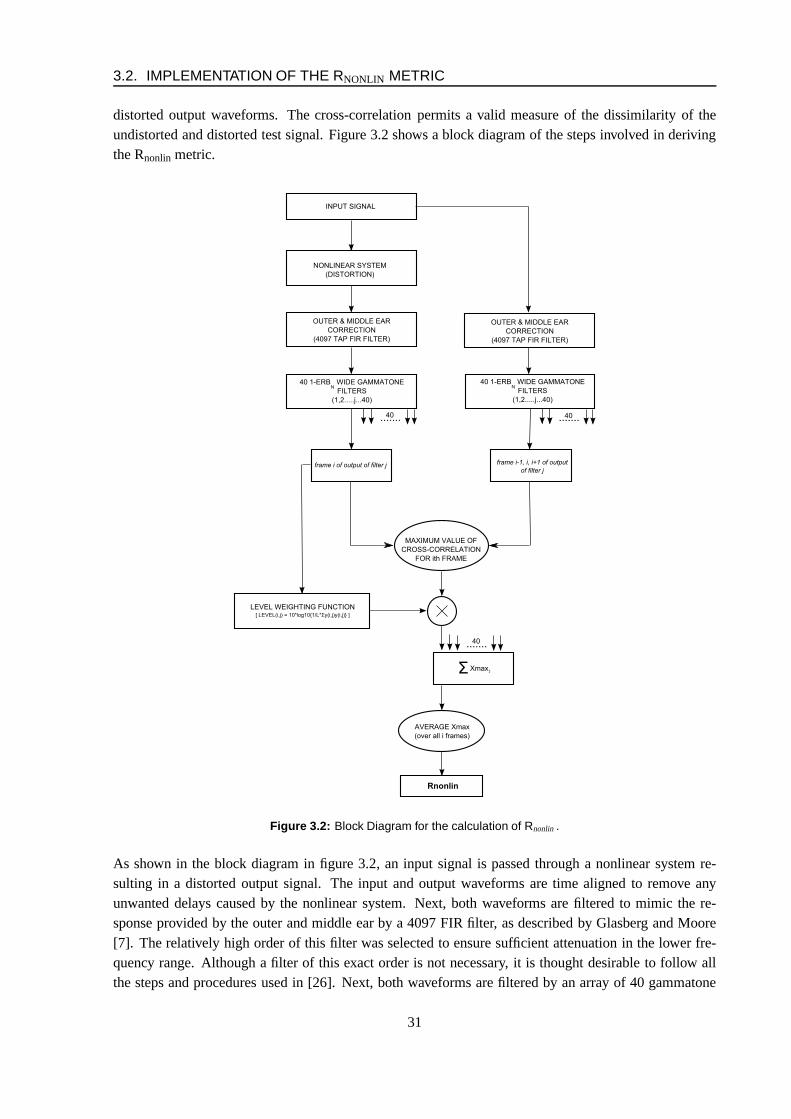
distorted output waveforms. The cross-correlation permits a valid measure of the dissimilarity of theundistorted and distorted test signal. Figure 3.2 shows a block diagram of the steps involved in derivingthe Rnonlin metric.

Figure 3.2: Block Diagram for the calculation of Rnonlin .

As shown in the block diagram in figure 3.2, an input signal is passed through a nonlinear system re-sulting in a distorted output signal. The input and output waveforms are time aligned to remove anyunwanted delays caused by the nonlinear system. Next, both waveforms are filtered to mimic the re-sponse provided by the outer and middle ear by a 4097 FIR filter, as described by Glasberg and Moore[7]. The relatively high order of this filter was selected to ensure sufficient attenuation in the lower fre-quency range. Although a filter of this exact order is not necessary, it is thought desirable to follow allthe steps and procedures used in [26]. Next, both waveforms are filtered by an array of 40 gammatone

31


filters with a bandwidth of 1-ERBN .

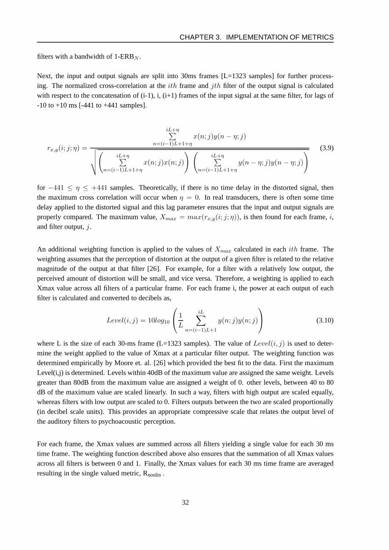
Next, the input and output signals are split into 30ms frames[L=1323 samples] for further process-ing. The normalized cross-correlation at theith frame andjth filter of the output signal is calculatedwith respect to the concatenation of (i-1), i, (i+1) frames of the input signal at the same filter, for lags of-10 to +10 ms [-441 to +441 samples].

rx,y(i; j; η) =

iL+η∑

n=(i−1)L+1+η

x(n; j)y(n − η; j)

√

√

√

√

(

iL+η∑

n=(i−1)L+1+η

x(n; j)x(n; j)

) (

iL+η∑

n=(i−1)L+1+η

y(n − η; j)y(n − η; j)

)

(3.9)

for −441 ≤ η ≤ +441 samples. Theoretically, if there is no time delay in the distorted signal, thenthe maximum cross correlation will occur whenη = 0. In real transducers, there is often some timedelay applied to the distorted signal and this lag parameterensures that the input and output signals areproperly compared. The maximum value,Xmax = max(rx,y(i; j; η)), is then found for each frame,i,and filter output,j.

An additional weighting function is applied to the values ofXmax calculated in eachith frame. Theweighting assumes that the perception of distortion at the output of a given filter is related to the relativemagnitude of the output at that filter [26]. For example, for afilter with a relatively low output, theperceived amount of distortion will be small, and vice versa. Therefore, a weighting is applied to eachXmax value across all filters of a particular frame. For each frame i, the power at each output of eachfilter is calculated and converted to decibels as,

Level(i, j) = 10log10

1

L

iL∑

n=(i−1)L+1

y(n; j)y(n; j)

(3.10)

where L is the size of each 30-ms frame (L=1323 samples). The value ofLevel(i, j) is used to deter-mine the weight applied to the value of Xmax at a particular filter output. The weighting function wasdetermined empirically by Moore et. al. [26] which providedthe best fit to the data. First the maximumLevel(i,j) is determined. Levels within 40dB of the maximumvalue are assigned the same weight. Levelsgreater than 80dB from the maximum value are assigned a weight of 0. other levels, between 40 to 80dB of the maximum value are scaled linearly. In such a way, filters with high output are scaled equally,whereas filters with low output are scaled to 0. Filters outputs between the two are scaled proportionally(in decibel scale units). This provides an appropriate compressive scale that relates the output level ofthe auditory filters to psychoacoustic perception.

For each frame, the Xmax values are summed across all filters yielding a single value for each 30 mstime frame. The weighting function described above also ensures that the summation of all Xmax valuesacross all filters is between 0 and 1. Finally, the Xmax valuesfor each 30 ms time frame are averagedresulting in the single valued metric, Rnonlin .

32

3.2. IMPLEMENTATION OF THE RNONLIN METRIC

To summarize, the Rnonlin metric calculates a time-averaged cross-correlation coefficient across the 40non-overlapping 1-ERBN filters. In such a manner, a more representative metric is derived, taking intoaccount the effects of the peripheral auditory system.

Outer-Middle Ear (OME) Filter

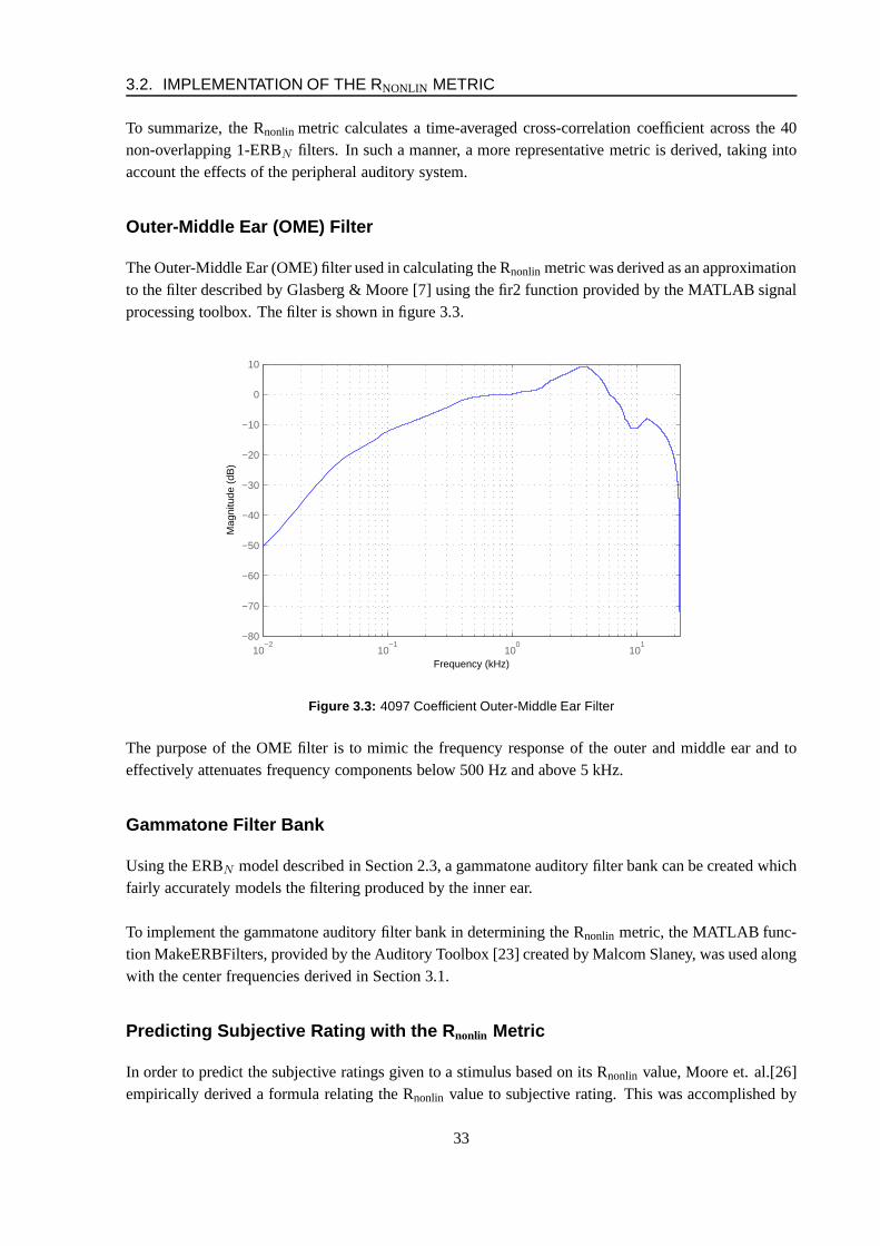
The Outer-Middle Ear (OME) filter used in calculating the Rnonlin metric was derived as an approximationto the filter described by Glasberg & Moore [7] using the fir2 function provided by the MATLAB signalprocessing toolbox. The filter is shown in figure 3.3.

10−2

10−1

100

101

−80

−70

−60

−50

−40

−30

−20

−10

0

10

Frequency (kHz)

Mag

nitu

de (

dB)

Figure 3.3: 4097 Coefficient Outer-Middle Ear Filter

The purpose of the OME filter is to mimic the frequency response of the outer and middle ear and toeffectively attenuates frequency components below 500 Hz and above 5 kHz.

Gammatone Filter Bank

Using the ERBN model described in Section 2.3, a gammatone auditory filter bank can be created whichfairly accurately models the filtering produced by the innerear.

To implement the gammatone auditory filter bank in determining the Rnonlin metric, the MATLAB func-tion MakeERBFilters, provided by the Auditory Toolbox [23]created by Malcom Slaney, was used alongwith the center frequencies derived in Section 3.1.

Predicting Subjective Rating with the R nonlin Metric

In order to predict the subjective ratings given to a stimulus based on its Rnonlin value, Moore et. al.[26]empirically derived a formula relating the Rnonlin value to subjective rating. This was accomplished by

33


102

103

104

−60

−50

−40

−30

−20

−10

0

Frequency (Hz)

Filt

er R

espo

nse

(dB

)

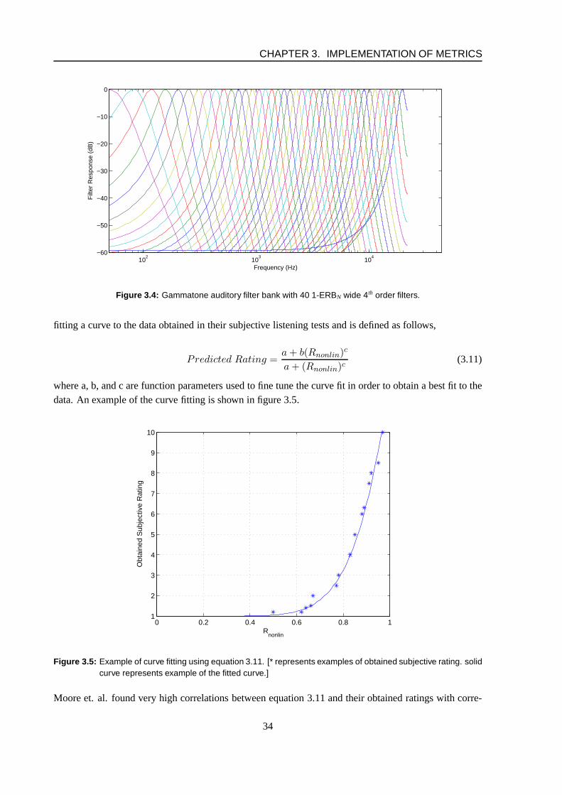
Figure 3.4: Gammatone auditory filter bank with 40 1-ERBN wide 4th order filters.

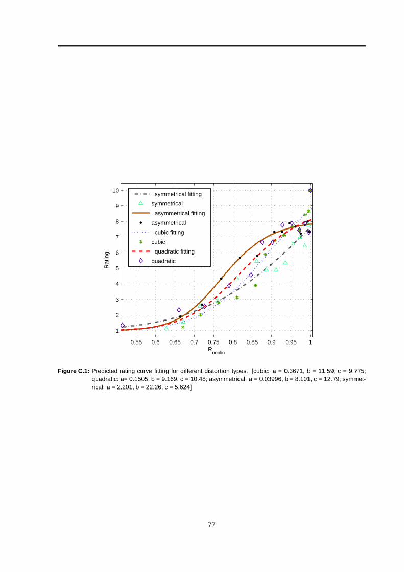
fitting a curve to the data obtained in their subjective listening tests and is defined as follows,

Predicted Rating =a + b(Rnonlin)c

a + (Rnonlin)c(3.11)

where a, b, and c are function parameters used to fine tune the curve fit in order to obtain a best fit to thedata. An example of the curve fitting is shown in figure 3.5.

0 0.2 0.4 0.6 0.8 11

2

3

4

5

6

7

8

9

10

Rnonlin

Obt

aine

d S

ubje

ctiv

e R

atin

g

Figure 3.5: Example of curve fitting using equation 3.11. [* represents examples of obtained subjective rating. solidcurve represents example of the fitted curve.]

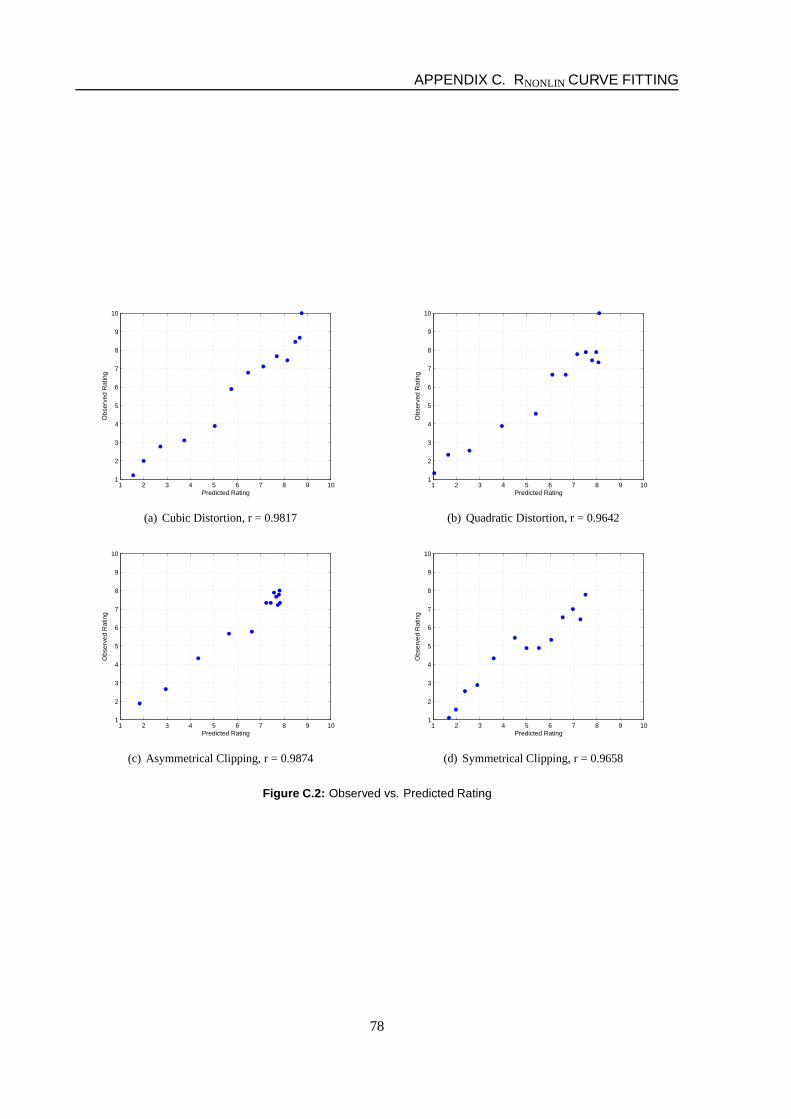
Moore et. al. found very high correlations between equation3.11 and their obtained ratings with corre-

34

3.3. IMPLEMENTATION OF THE THD & IMD METRICS

lation coefficients as high as 0.98 [26]. Therefore, by usingequation 3.11, a prediction of the subjectiverating due to a particular type of distortion may be obtainedwith relatively high accuracy.

3.3 Implementation of The THD & IMD Metrics

The THD and IMD metrics will also be provided in this chapter.This serves to verify the poor correlationof these metrics in comparison with the new DS and Rnonlin metrics.

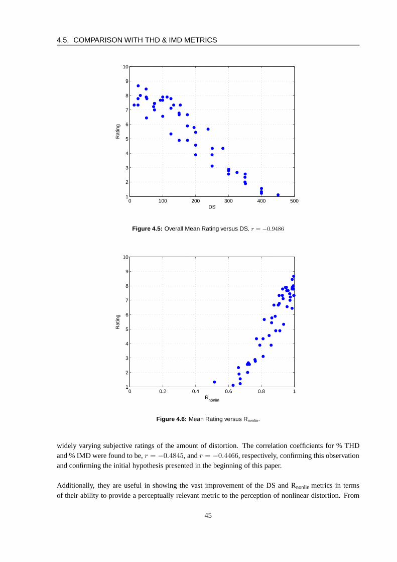
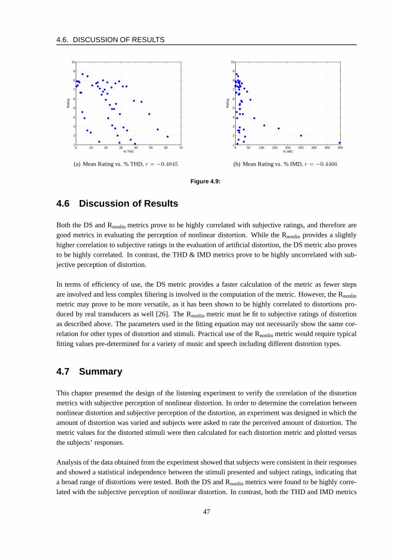
The implementation of these metrics was not trivial. This stems from the fact that the THD and IMDmetrics are dependent on the amplitude of the input test signal. Furthermore, most THD and IMD in-put test signals are selected to be at least 10 dB below clipping levels. This requirement does not suitthe needs of this project as clipping has been artificially added to a music sample and it is of interestto obtain the THD or IMD values describing how much distortion these clippings introduce. As such,the amplitude for the input test signal to arrive at appropriate THD and IMD values for the nonlinearsystems described in this chapter is the peak value of the undistorted music sample. It should be notedthat comparison between the THD and IMD values presented in this report is not valid between THDand IMD values presented by other researchers unless the same input test signal conditions apply.

Description of the THD+N Algorithm

The THD+N method was implemented in MATLAB as outlined in Section 2.4. The input test signal wasfixed at 1 kHz with an amplitude corresponding to the peak value of the undistorted music sample. Thesampling frequency of the input test signal was 44.1 kHz witha 1 second duration. The test signal wasthen passed through each of the nonlinear distortion systems. To compute the numerator of equation 3.12a notch filter (FIR 1000 taps) centered around 1 kHz was used toremove the fundamental component ofthe test signal leaving only harmonic components. The first 2000 samples of the output signal from thenotch filter were removed to reduce the effects of the filter onthe overall rms output. Removing the first2000 taps is not necessary as only the first 1000 samples wouldcontain effects from the filter. However,the first 2000 samples were removed so as to be well beyond any effect from the filter.

%THD = 100

√

V 22 + V 2

3 + V 24 + ...V 2

n

VT(3.12)

Description of the IMD Algorithm

The IMD method was implemented in MATLAB according to the CCIF method described in Section 2.4.The sampling frequency of the input test signal was 44.1 kHz with a 1 second duration. The two tonesof the input signal were set to 14 and 15 kHz. The selection of these frequencies reduces the injectionof harmonic components and the higher intermodulation products. The rms sum between the distortionproducts was evaluated and expressed as a ratio against the rms value of the input signal. The rms sum ofthe distortion products was calculated by removing the two input frequencies using two cascaded notch

35


filters (FIR 300). The first 1000 samples of the output signal from the two cascaded notch filters wereremoved to reduce the effect of the FIR filter on the overall rms output.

3.4 Summary

The DS metric was presented at the beginning of the chapter. The DS metric is essentially the averageof the power level differences between the output spectrum from a nonlinear device and the originalundistorted input test signal across 40 non-overlapping ERBs. The input test signal is a 10 componentmultitone signal. The method of arriving at the appropriatecenter frequencies for the 40 non-overlappingERBs required for the DS computation was also detailed.

The implementation of the Rnonlin metric was further discussed. The Rnonlin metric is based of the cross-correlation between the original undistorted input test signal and the resulting distorted output from anonlinear device. The metric algorithm models the auditorysystem by taking into account the filteringproduced by the outer and middle ear and the filtering of the auditory system. A weighting factor is alsoused in the metric which is based on the assumption that the perception of distortion from the output of agiven auditory filter is related to the magnitude of the output from that filter. The methods of predictingsubjective ratings of nonlinear distortion using the Rnonlin metric were also discussed.

The THD+N and IMD algorithms were presented at the end of the chapter and implemented in MATLAB.The input signal used to arrive at both metrics was set to the peak value of an undistorted music samplewhich is used in the following chapter. The following chapter relates the presented metrics to subjectiveratings of nonlinear distortion.

36

CHAPTER 4

EXPERIMENT 1: VERIFICATION OF

M ETRICS

This chapter provides an overview of the listening experiment conducted to verify the correlation of theDS and Rnonlin metrics with subjective perception of nonlinear distortion. The design of the listeningtest is presented along with a description of the test stimuli and the steps involved in their creation. Ananalysis of the results is then presented along with the verification of the metrics using the obtained data.

4.1 Listening Evaluation to Determine Subjective Ratings o f Non-linear Distortion Systems

The research of [25] and [26] collected subjective ratings of distortion for a wide variety of nonlinearsystems using both artificially applied distortion and distortion produced by real transducers. These sub-jective ratings were used to arrive at the proper algorithm settings for for the DS and Rnonlin metrics.The metric algorithms were implemented as described in the previous sections. However, it was founddifficult to verify that they were implemented correctly without checking their correlation with somesubjective ratings. Therefore, a small listening experiment was designed to "check" if these metric algo-rithms were in fact implemented correctly. By correctly implemented, it is meant that these metrics arehighly correlated with the subjective ratings. For the purposes of the the distortion threshold evaluation,it is imperative that these metrics are well correlated withsubjective ratings.

The purpose of the listening experiment was to be a "check" ofthe implemented metric algorithms andtherefore it was designed to be short for an individual subject. The test was designed to be approximately6 minutes in duration. Within the short session the subjective would rate the level of distortion on a scalefrom 1 - 10 where 10 would refer to an undistorted signal and 1 acompletely distorted signal. Beforeallowing the subject to rate the distorted stimuli, the subjects were presented with signals correspondingto a 1 and 10. This rating procedure was same as used in [25].

A total of four nonlinear systems were selected for the purposes of this metric verification listeningevaluation. These systems are:

1. Hard asymmetrical clipping.

37

CHAPTER 4. EXPERIMENT 1: VERIFICATION OF METRICS

Vf Clipping Factor (Vp/Vf) Asymmetrical Clipping Symmetrical ClippingDS DS

1.48 13.244 25.0591.615 32.103 50.8161.74 51.846 75.1091.873 72.408 100.072.01 93.016 125.032.155 113.21 150.092.315 133.36 175.372.49 153.42 200.082.92 195.18 250.693.5 237.82 300.644.37 282.78 350.685.91 325.81 400.210 351.6 450.57

Table 4.1: Table showing clipping levels and DS values for asymmetrical and symmetrical clippings.

2. Hard symmetrical clipping.

3. Squared distortion described byy = αx2 + x.

4. Cubic distortion described byy = βx3 + x.

A sample of guitar music of 4.4 second duration was selected as the input signal to these distortion sys-tems. This wave file segment was taken from the CD "Sound Quality Assessment Material" (SQAM)produced by the European Broadcasting Union. The music sample has a relatively constant overall signallevel without major peaks which could dominate the overall perceived distortion.

The clipping levels for the hard symmetrical clipping were found by dividing the peak value of the inputsignal,Vp, by a factorVf . The clipping levels for the hard symmetrical clipping wereset to yield DSvalues of 25, 50, 75, 100, 125, 150, 175, 200, 250, 300, 350, 400 and 450. These same clipping levelswere used for the asymmetrical clipping level which yieldedsomewhat different DS values. The clippinglevels and corresponding DS values are shown below in table 4.1 for both the asymmetrical and sym-metrical distortion systems. During pilot experiments performed on group members it was found thatdistortion levels between 25-200 DS were often hard to perceive. For this reason, more points betweenDS values from 25-200 were selected.

For both the squared and cubic distortion systems, the coefficientsα andβ were adjusted to yield DSvalues of 25, 50, 75, 100, 125, 150, 175, 200, 250, 300, 350, 400. The coefficientsα andβ are shown intable 4.2 with their the corresponding DS values. While applying the polynomial distortion systems, spe-cial care was taken to ensure that peak levels in the signal did not exceed 1 or -1. The functionwavwrite

provided by MATLAB clips all peaks exceeding 1 or -1.

Figure 4.1 shows the input-output relationships for the above nonlinear systems. For graphical purposes,the input signal used to make these graphs was not the input signal from SQAM. Rather, a signal linearlyspaced between -.2 and .2 was used. The 0.2 was chosen as this was the peak value of the guitar signaldescribed above. The asymmetrical clipping is plotted for DS levels of 13, 153, and 351. The symmet-rical clipping is plotted for DS levels of 25, 200 and 450. Thesquared distortion type is plotted for DS

38

4.1. LISTENING EVALUATION TO DETERMINE SUBJECTIVE RATINGS OF NONLINEARDISTORTION SYSTEMS

Squared Distortion Cubic DistortionDS Alpha Beta

25.059 0.245 2.750.816 0.48 5.275.109 0.75 8.3100.07 1.04 11.8125.03 1.36 16150.09 1.72 20.8175.37 2.1 26.6200.08 2.55 33.3250.69 3.56 50.6300.64 4.98 75.6350.68 6.9 114.6400.2 13.4 181.5

Table 4.2: Table showing coefficient values and DS values for squared and cubic distortions.

values of 25, 200 and 400. At lower DS values, the squared factor is less significant and the resulting in-put output relationship shows a kind of soft asymmetrical clipping for values below 0. As the coefficientα increases, the squared polynomial dominates the waveform as demonstrated by the parabolic function.The cubic function is somewhat similar. As the coefficientβ increases the cubic function takes over.

−0.2 −0.1 0 0.1 0.2−0.2

−0.1

0

0.1

0.2

Input x

Oup

ut y

Hard Asymmetrical Clipping

−0.2 −0.1 0 0.1 0.2−0.2

−0.1

0

0.1

0.2

Input x

Out

put y

Hard Symmetrical Clipping

−0.2 −0.1 0 0.1 0.2−0.2

−0.1

0

0.1

0.2

Input x

Out

put y

Squared Distortion

−0.2 −0.1 0 0.1 0.2−0.2

−0.1

0

0.1

0.2

Input x

Out

put y

Cubic Distortion

Figure 4.1: Input-Output relationships for nonlinear systems using input signal described above.

The input signal was distorted by each of the above systems and the output was stored as a stereo wavefile where each channel contained the same signal. A total of 50 stimuli were created for the purposes ofthe subjective listening evaluation.

When evaluating a psychophysical percept such as the perceived amount of nonlinear distortion in astimulus, it is important to isolate the percept. Therefore, in order to eliminate the effects of linear distor-

39


tion introduced by each of distortion types, a loudness normalization was applied to each of the stimuli.In such a way, any linear gain or attenutation introduced will not effect the subjects responses. This isparticularly important when evaluating multiple stimuli on the same subjective scale (i.e. 1 to 10). Thelevel of one stimulus in comparison with the next could influence the subject’s response in an undesirableway. By normalizing the loudness of all stimuli, the only difference between the original signal and thedistorted signal is the due to the applied nonlinear distortion. For example, clipping the signal by a anyfactor will reduce the overall level of the signal. Therefore, some gain should be applied to the clippedsignal to ensure the distorted signal has the same overall loudness as the original signal, as well as thesame overall loudness as all other distorted signals.

The loudness normalization was performed using a MATLAB program that implements the DIN 45631/ ISO532B standard based on Zwicker’s loudness model (see Appendix B). Each of the 50 stimuli werenormalized to have an overall loudness of approximately 15 sones (plus or minus .5 sone). As the loud-ness model uses a third-octave band analysis to approximatethe ear’s frequency selectivity, it is importantto take into account the effect that the headphone’s frequency response will have on the resulting loud-ness. As the headphone’s frequency response is not flat (Appendix A.2), it will alter certain frequenciesmore than others. Therefore, before calculating the loudness of the distorted stimuli, they were firstfiltered by an average of the headphone’s left cup impulse response. The resulting loudness was thencalculated. If the overall loudness caluculated was not 15 sones, an amplitude scaling factor was thenapplied to the original stimuli, and the loudness calculation process repeated, until the appropriate sonelevel was achieved. This scaling factor was then used to scale the original, unfiltered stimulus and theresulting waveform written to a stereo .wav file. The loudness model assumes that the input signal is inPascals, however the signal is not in Pascals and the sone value specified here is not truly representativeof the actual loudness. However, as all stimuli will pass through the same reproduction chain, and themodel is used only to normalize the stimuli to the same loudness level, this consideration will not effectthe normalization process. Figure 4.2 shows the block diagram of the processing involved in creating alldistorted stimuli.

Figure 4.2: Block diagram showing the processing of the original, undistorted signal to the distorted version usedin listening tests.

A MATLAB graphical user interface (GUI) was created to interface with the subject. As mentionedearlier, the subject is presented with the undistorted and most distorted signal before proceeding with thesubjective evaluation. The subject was able to listen to both scale extremes as many times as they wantedbefore beginning with the test. The most distorted signal (case 1) was selected as the signal having thehighest DS value and the lowest the original undistorted signal (case 10). The highest DS value corre-sponded to the most extreme case of the symmetrical clipping. A screenshot of the GUI used for theevaluation is shown below in figure 4.3. The GUI program presents the 50 stimuli in random order andstores the subject’s response and the file name of the presented stimulus for further statistical analysis.

40

4.1. LISTENING EVALUATION TO DETERMINE SUBJECTIVE RATINGS OF NONLINEARDISTORTION SYSTEMS

Figure 4.3: Graphical user interface for DS verification listening test.

The signals were presented to the subject after clicking on the selected rating. Case 10, the undistortedsignal, was never presented to the subject during the experiment. Each stimulus was presented only oncewithin the session since the design of the experiment was to make it relatively short in duration.

The listening evaluation was performed in a small listeningcabin in the Acoustic Laboratory at AalborgUniversity. The subjects ranged in ages from 21 to 26 years. The stimuli were presented to the sub-jects through a pair of Beyerdynamic DT990 headphones whichwere connected directly to a PC soundcard. Nonlinear distortion measurements were performed onthe sound reproduction chain prior to thelistening evaluations (Appendix A.1). The overall signal level presented to the subjects was 70 dBA, orappoximtely 20 sones (DIN 45631/ISO532B). The loudness measurement description can be found inAppendix B on page 73 along with relavent equipment information and the instruction sheet given to thesubjects before the evaluation.

A total of nine subjects were used for this experiment excluding group members. The subjects wereall 10th semester Acoustic’s students. It should be noted that one of two subjects felt that certain typesof distortion were perceived as being more distorted than the extreme case (DS 450 from symmetricalclipping). This was later found to be of little consequence as most subjects rated this signal as having thehighest distortion.

41


4.2 Analysis of Results

Analysis of Variance

An analysis of variance (ANOVA) was performed on the subjective ratings given by all subjects withrespect to the amount of distortion. The ANOVA analysis provides a means of evaluating the variancebetween groups, or in this case, the variance between the subjects’ ratings for the different amounts ofdistortion. More specifically, it is assumed that the mean subjective rating for different levels of DS aredifferent. The ANOVA analysis is used to either accept or reject the null hypothesis. The null hypothesisfor the evaluation of the variance between the subjective ratings at different distortion levels is that theiroverall mean is the same. For example, if the mean subjectiveratings at 50 DS are equal to the overallmean rating at 200 DS, then the null hypothesis would be true.To support the aforementioned assump-tion, the null hypothesis must be rejected.

The ANOVA analysis yields two parameters, F and p-value, which can be used to evaluate the signifi-cance. The F parameter is defined below.

F =(found variation of the group averages)

(expected variation of the group averages)(4.1)

The null hypothesis would be correct is the F value is closer to 1. This F ratio is used to test for a statisti-cal significance, or p-value. The p-value refers to the probability that a variate would have a value greaterthan or equal to the value observed by chance. For example, a p-value [p < .01] would indicate that themeans differ by more than what would be expected by chance. Inthis case, the null hypothesis can berejected. The null hypothesis, for the purposes of this project, is rejected for [p < .05] (95% confidenceinterval).

The analysis performed on the obtained data showed that the subjective ratings were highly significant[F = 23.51, p < 0.0001].

Additionally, for each type of distortion (i.e. asymmetrical, symmetrical, quadratic, cubic), a Two-WayANOVA was performed on the subjective rating with amount of distortion and subject as factors. Foreach type of distortion it was found that the amount of distortion was significant [p < 0.0001 for all typesof distortion]. For subjects as a factor there was only one case in which the subject was not significant[p = .0125]. This occurred for the asymmetrical clipping group. This indicates that the overall meansubject ratings for all distortion levels within this groupwhere sometimes different between subjects.

The Two-Way analysis is an extended version of the one way analysis which is based on the followingnull hypotheses:

1. The means of the first factor are equal (level of distortion).

2. The means of the second factor are equal (subject).

3. There is no interaction between the two factors. This is not applicable as there are not repeatedobservations for both factors.

42

4.3. VERIFICATION OF DS METRIC

Consistency Across Subjects

In order to assess the consistency across the subjects, the mean values of the subjective ratings were cal-culated for each stimulus and compared to the rating given bya particular subject for the given stimulus.This resulted in a correlation coefficient comparing the subjective ratings given by a particular subjectagainst the overall mean values given by all subjects. Table4.3 shows these correlation coefficients forall 9 subjects and shows a fairly high consistency across allsubjects. The standard deviation, SD, ofthe subjective ratings across all subjects was 1.4 scale units which is relatively consistent with the SDobtained by Moore et. al. [25].

Subject ALE ANT CAR CAS DAV IRE LAR LRM YES

Correlation Coefficient 0.85 0.90 0.85 0.91 0.92 0.80 0.77 0.92 0.88

Table 4.3: Correlation of subjective ratings for individual subjects with mean value of subjective ratings across allsubjects.

4.3 Verification of DS Metric

The mean values of the subjective ratings for each of the distortion types were computed and are shownin figure 4.4. Additionally, the overall mean values of the subjective ratings were computed for all stimuliand are shown in figure 4.5. The DS metric and the subjective ratings were found to be highly corre-lated with a negative correlation of−0.9486. This correlation is consistent with the correlation foundbyMoore et. al. [25] of−0.95 for artificial distortion applied to a music stimulus.

4.4 Verification of R nonlin Metric

The mean values of the subjective ratings are plotted against the Rnonlin metric in figure 4.6.

As described by Moore et. al. [26], a curve fitting may be applied to the data using the empiricallyobtained formula,

Predicted Rating = (a + bRc

nonlin

a + Rcnonlin

) (4.2)

where a,b, and c are function parameters used to fine tune the curve to achieve the best fit, as described insection 3.2. The fitted curve is shown in figure 4.7. The fitted curve was determined to have a reasonablefit, with an adjusted-R2 value of0.9295.

Using the curve fitting equation described by equation 4.2, the predicted values of the subjective ratingsmay be calculated. Figure 4.8 shows a plot of the observed versus the predicted values of the subjec-tive ratings found using equation 4.2. It was determined that the observed versus predicted ratings were

43


0 50 100 150 200 250 300 350 400 4501

2

3

4

5

6

7

8

9

10

Rat

ing

DS

(a) Cubic distortion.r = −0.9778

0 50 100 150 200 250 300 350 400 4501

2

3

4

5

6

7

8

9

10

Rat

ing

DS

(b) Quadratic distortion.r = −0.9556

0 50 100 150 200 250 300 350 400 4501

2

3

4

5

6

7

8

9

10

Rat

ing

DS

(c) Asymmetrical clipping.r = −0.9282

0 50 100 150 200 250 300 350 400 4501

2

3

4

5

6

7

8

9

10

Rat

ing

DS

(d) Symmetrical clipping.r = −0.9791

Figure 4.4: Mean Rating versus DS.

highly correlated with a correlation coefficient of0.9547.

The individual Rnonlin fittings for each type of distortion along with plots of predicted ratings can befound in Appendix C.

4.5 Comparison with THD & IMD Metrics

In order to judge the performance of the DS and Rnonlin metrics with respect to the traditional metrics,corresponding THD and IMD values were calculated from the data obtained from the listening test. Sec-tion 3.3 describes the process used to obtain the corresponding values of THD and IMD. Figures 4.9(a)and 4.9(b) show the resulting mean subjective ratings versus % THD and % IMD, respectively. As be-fore, mean ratings can take the values from 10 (undistorted)to 1 (completely distorted), and increasingvalues of % THD and % IMD imply increasing levels of distortion.

Not surprisingly, both figures show that the metrics are not correlated with any perceptual rating of dis-tortion. Of particular note, is that for both THD and IMD, similar values of a particular metric result in

44

4.5. COMPARISON WITH THD & IMD METRICS

0 100 200 300 400 5001

2

3

4

5

6

7

8

9

10

DS

Rat

ing

Figure 4.5: Overall Mean Rating versus DS. r = −0.9486

0 0.2 0.4 0.6 0.8 11

2

3

4

5

6

7

8

9

10

Rnonlin

Rat

ing

Figure 4.6: Mean Rating versus Rnonlin.

widely varying subjective ratings of the amount of distortion. The correlation coefficients for % THDand % IMD were found to be,r = −0.4845, andr = −0.4466, respectively, confirming this observationand confirming the initial hypothesis presented in the beginning of this paper.

Additionally, they are useful in showing the vast improvement of the DS and Rnonlin metrics in termsof their ability to provide a perceptually relevant metric to the perception of nonlinear distortion. From

45


0 0.2 0.4 0.6 0.8 11

2

3

4

5

6

7

8

9

10

Rnonlin

Rat

ing

Figure 4.7: Curve fitting of mean rating versus Rnonlin. Solid curve represents the fitted curve obtained using theequation Predicted Rating =

(a+bRc

nonlin)

(a+Rc

nonlin)

, where a = 0.1674, b = 9.063, c = 10.1

1 2 3 4 5 6 7 8 9 101

2

3

4

5

6

7

8

9

10

Predicted Rating

Obs

erve

d R

atin

g

Figure 4.8: Predicted Rating versus Observed Rating obtained using the fitted curve shown in figure 4.7. r = 0.9547

this, it can be concluded that both the THD and IMD metrics arecompletely insufficient metrics fordescribing the perceptual effects of nonlinear distortionand are therefore excluded from any furtherevaluation in the remainder of this paper.

46

4.6. DISCUSSION OF RESULTS

0 10 20 30 40 50 60 701

2

3

4

5

6

7

8

9

10

% THD

Rat

ing

(a) Mean Rating vs. % THD,r = −0.4845

0 50 100 150 200 250 300 350 4001

2

3

4

5

6

7

8

9

10

% IMD

Rat

ing

(b) Mean Rating vs. % IMD,r = −0.4466

Figure 4.9:

4.6 Discussion of Results

Both the DS and Rnonlin metrics prove to be highly correlated with subjective ratings, and therefore aregood metrics in evaluating the perception of nonlinear distortion. While the Rnonlin provides a slightlyhigher correlation to subjective ratings in the evaluationof artificial distortion, the DS metric also provesto be highly correlated. In contrast, the THD & IMD metrics prove to be highly uncorrelated with sub-jective perception of distortion.

In terms of efficiency of use, the DS metric provides a faster calculation of the metric as fewer stepsare involved and less complex filtering is involved in the computation of the metric. However, the Rnonlin

metric may prove to be more versatile, as it has been shown to be highly correlated to distortions pro-duced by real transducers as well [26]. The Rnonlin metric must be fit to subjective ratings of distortionas described above. The parameters used in the fitting equation may not necessarily show the same cor-relation for other types of distortion and stimuli. Practical use of the Rnonlin metric would require typicalfitting values pre-determined for a variety of music and speech including different distortion types.

4.7 Summary

This chapter presented the design of the listening experiment to verify the correlation of the distortionmetrics with subjective perception of nonlinear distortion. In order to determine the correlation betweennonlinear distortion and subjective perception of the distortion, an experiment was designed in which theamount of distortion was varied and subjects were asked to rate the perceived amount of distortion. Themetric values for the distorted stimuli were then calculated for each distortion metric and plotted versusthe subjects’ responses.

Analysis of the data obtained from the experiment showed that subjects were consistent in their responsesand showed a statistical independence between the stimuli presented and subject ratings, indicating thata broad range of distortions were tested. Both the DS and Rnonlin metrics were found to be highly corre-lated with the subjective perception of nonlinear distortion. In contrast, both the THD and IMD metrics

47


were found to be uncorrelated with the subjective perception of nonlinear distortion.

With the DS and Rnonlin metrics verified as being correlated with the perception of distortion, the metricsmay be used to investigate other perceptual properties of nonlinear distortion. Therefore, the threshold ofaudibility of nonlinear distortion may be investigated with a metric related to the perception of nonlineardistortion which was never before available with the conventional metrics.

48

CHAPTER 5

EXPERIMENT 2: DETERMINATION OF

NONLINEAR DISTORTION THRESHOLDS

This chapter documents the methods used to obtain nonlineardistortion thresholds for four types ofnonlinear distortion systems. The design of the experimentis first presented detailing the distortion typesand music stimuli used. Details of the performed listening evaluations are also given. The chapter alsopresents a statistical analysis of the results.

5.1 Thresholds of Nonlinear Distortion

A listening test was designed to find the point at which nonlinear distortion is "just audible," or in otherwords, the threshold of perception of nonlinear distortion. In order to design the listening test, an ap-propriate metric is needed to serve as the dependent variable which is varied during the test. In the caseof finding the thresholds for different kinds of distortion it was selected to use the DS metric as the de-pendent variable. The DS metric was chosen as it is the most physical metric of the metrics discussedin this report in the sense that it incorporates very little psychoacoustic modeling in deriving the metric.Therefore the DS metric, while an improved metric over such metrics as THD and IMD, still provides aphysical measurement of the amount of distortion in a signal.

In experiment 1, the DS metric was found to be linear with respect to subjective perception of distortion.As the DS value increased, the perception of the distortion increases proportionally. Using a linear metricprovides the advantage of making it easier to determine the threshold, since a linear interpolation methodmay be applied in deriving the threshold value.

In such a way, varying the DS metric provides a way of varying the physical amount of distortion inthe signal. Once the threshold is determined, the DS value for this threshold can easily be mapped to acorresponding Rnonlin value from the transfer function and its corresponding parameters which have beencomputed a priori. It is highlighted that the DS and Rnonlin values are derived directly from a nonlineartransfer function and it is not possible to map a DS value directly to a Rnonlin value without knowledge ofthe transfer function.

49

CHAPTER 5. EXPERIMENT 2: DETERMINATION OF NONLINEAR DISTORTIONTHRESHOLDS

Experimental Design

In order to find the threshold of nonlinear distortion, an appropriate psychometric design is needed toprovide both accurate and repeatable results. Traditionally, threshold experiments are conducted usinga single stimulus which is varied according to some physicalparameter in question. Subjects are thenpresented with the stimuli and must respond when the subjective response to the parameter in questionis perceived by the subject. This results in both positive (correct) and negative (incorrect) responses withrespect to the varying parameter.

In this experiment, however, the traditional single stimulus procedure is not desirable as there is no ref-erence stimulus with which subjects can base their responses. Therefore, a 2 Alternative Forced Choice(2AFC) paradigm was used. This procedure is preferred over the traditional one stimulus procedure, asthe understanding of the concept of distortion is not alwayswidely understood. In the 2AFC method, asubject is presented with both a distorted stimulus along with the undistorted or reference signal. Thesubject is then asked to determine which of the two stimuli isthe distorted stimulus.

It is desired to design a test that is both accurate and efficient in its implementation, therefore an ap-propriate algorithm should be selected that fulfills both ofthese requirements. Several commonly usedpsychometric methods include the method of constants, the method of limits, simple up-down method,and the transformed up-down method, the latter two being themost common among them.

Traditionally, the methods described above are conducted using stimuli whose parameters are varied bya constant factor, or step size. In such a way, subsequent stimuli are varied according to the step sizeuntil the threshold is reached. While this method is accurate, it is not necessarily efficient. If the regionwhere the threshold lies is unknown, this procedure may takea long time to converge to the threshold.Using an adaptive procedure, or a procedure in which the stepsize is varied based on subject responses,provides a more efficient method of determining the threshold. Using such a method, one can initializethe test using a large step size and as responses are recorded, the step size may vary accordingly. It hasbeen shown that this adaptive method of reducing the step size leads to a maximal rate of convergence tothe desired threshold value. [11]

Algorithm Implementation

An adaptive transformed up-down algorithm with descendingdistortion scores (i.e. starting with verydistorted signals) was selected due to its accuracy and efficiency. The choice between descending orascending starting points in an up-down method is importantdue to subject biasing, known as hysteresis.When a subject is presented with stimuli with descending level, it is possible for the a subject to continueperceiving an effect even after it is physically gone. Conversely, when a subject is presented with stimuliwith increasing level, a subject may not perceive the increase in level until a marked increase in level hasoccurred, which may be beyond the threshold. In this fashion, a descending experiment will always yielda lower threshold than an ascending experiment. Up-Down methods have the advantage of limiting thisbias to a certain extent due to the fact that it converges to the threshold from both sides. It was decidedthat beginning the test with an audible example of the effects of distortion on the particular sample wasimportant in allowing the subject time to perceive the effects of distortion on the test signal, and therefore

50

5.2. TEST IMPLEMENTATION

a descending starting point was chosen.

The initial step size of the test was selected to be 25 DS, withsubsequent step sizes of 10 DS and 5DS after the 1st and 3rd reversals, respectively. The resulting resolution of 5 DS was found to be suitablefrom past experience. Additionally, the cross-correlation coefficient was also calculated for two signalsdiffering by a value of 5 DS and was found to have a maximum value of 0.9985, leading to the assump-tion that a difference in 5 DS of two given signals provides a high resolution. The test was terminatedafter 6 reversals. It is recommended to use at least 6-8 reversals, but using 6 has the added advantage ofreducing the duration of the experiment which reduces subject fatigue.

The initial starting DS was determined empirically in a pilot test. As stated before, it was thought tobe important to give the subjects an initial impression of examples of distorted signals. Therefore, foreach test case, a DS value was found where the distortion was clearly evident.

Experimental Stimuli

It was shown in the previous experiments, that while the DS and Rnonlin metrics are well correlated withsubjective ratings for the perceived amount of distortion,it can not be assumed that each type of distor-tion will have the same threshold. Therefore it was decided to test the threshold for each of the four typesof distortion described in section 4.1 independently.

It was desired to investigate the influence of the type of stimulus used on the measured thresholds andtherefore two stimuli were used for each of the four distortion types to be investigated, resulting in eightseparate cases. The two stimuli were chosen to both have a relatively constant overall level, but withslightly different time and frequency content. The stimuliselected were a jazz excerpt from the song"Charles Christopher" by the Phil Woods Trio off the Chesky Records Audiophile Test CD [21] and aclassical excerpt from "Lyric Andante" by Reger taken from the AAU High Fidelity Reference CD#2[28]. A spectrogram of each excerpt is shown in figure 5.1.

The main difference between the musical excerpts in figures 5.1(a) and 5.1(b) is that the jazz excerptcontains more transients than does the classical excerpt, and that overall time-frequency content of theclassical excerpt is more constant.

5.2 Test Implementation

As eight cases were to be evaluated during the test, it was decided to split the test into two groups inorder to reduce the duration of the complete experiment. Thetwo groups were divided into a polynomialdistortion group and a hard clipping group. It was calculated that each group would require approxi-mately 45 minutes from a subject. Each group consisted of four test sessions to evaluate the thresholdof distortion for each type of distortion in the group. Table5.1 shows the two groups and the test ses-sions involved. Within each group, a database of stimuli were created which contained distortion levelsvarying in increments of 5 DS from 0 to 200 DS. The maximum level of 200 DS was selected as it wasclearly audible as confirmed by pilot test subjects. As in theprevious experiment, all stimuli were loud-

51


Fre

quen

cy [k

Hz]

0

5

10

15

20

−120

−100

−80

−60

−40

−20

0

20

0 1 2 3 4 5

−0.2

0

0.2

Am

plitu

de

Time [s]

(a) Spectrogram for jazz excerpt

Fre

quen

cy [k

Hz]

0

5

10

15

20

−150

−100

−50

0

0 1 2 3 4 5

−0.2

0

0.2

Am

plitu

de

Time [s]

(b) Spectrogram for classical excerpt

Figure 5.1: Spectrograms for music excerpts.

ness normalized to the same level.

test session Group 1 Group 21 Cubic distortion applied to classical music sample Symmetric hard clipping applied to classical music sample2 Cubic distortion applied to jazz music sample Symmetric hard clipping applied to jazz music sample3 Quadratic distortion applied to classical music sampleAsymmetric hard clipping applied to classical music sample4 Quadratic distortion applied to jazz music sample Asymmetric hard clipping applied to jazz music sample

Table 5.1: Division of groups in the listening test.

A total of twelve subjects participated in the listening experiment, where six evaluated Group 1, and sixevaluated Group 2. Each subject was screened with an audiometry prior to the test to ensure that theyhad no hearing loss greater than 20 dB HL. Each test subject was then given a set of instructions for thetest, as well as a questionnaire in order to assess any other possible history of hearing impairments thatcould adversely affect the test.

A Graphical User Interface (GUI) was programmed in MATLAB tointerface with the subjects. A screen-

52

5.3. RESULTS FROM THE THRESHOLD EXPERIMENTS

Figure 5.2: GUI for threshold experiment.

shot of the GUI is shown in figure 5.2. Prior to the test sessions, a brief training session was conductedwhere the subjects were presented with two extreme examplesof the type of 2AFC comparisons theywould hear during the test sessions. Extreme examples were used where the distorted signals presentedwere the most severe cases they would encounter and the distortion was clearly evident. This was done toensure that the subjects were familiar with the concept of distortion as well as to familiarize the subjectwith the types of signals that would be evaluated during eachtest sessions. After the training session, themain test began. Subjects were allowed breaks between each of the four test sessions.

5.3 Results from the Threshold Experiments

Before describing the procedure used to arrive at the estimation of the threshold,X70, two examplesof the transformed up-down procedure used during the experiments are presented. Figure 5.3 plots theresults from experiment A using cubic distortion and figure 5.4 experiment B using symmetrical hardclipping both applied to a sample of classical music. It is re-iterated that a different subject was usedfor each experiments. In the figures below, descending values values of DS indicate decreasing levels ofdistortion.

From figure 5.3 it can be noted that the initial DS level is at 120 which decreases in steps of 25 to 45DS at trial number 7. This point is the first reversal reached during the experiment. The DS level returnsto the level preceding the reversal point from which the stepsize is changed to 10 DS for the next tworeverals. The third reversal occurs at trial 16 from which point the step size changes to its final value of5 DS. Referring to experiment B in figure 5.4 it is noted that the initial DS level is at 100. As was seenwith almost all of the hard clipping distortion threshold experiments, the first reversal occured at DS 0.

53


0 5 10 15 20 2540

50

60

70

80

90

100

110

120

Trial (n)

DS

Cubic Distortion Classical Music (Subject: ’RAU’)

Figure 5.3: Experiment A: cubic distortion applied to classical music sample.

0 5 10 15 20 25 30 350

20

40

60

80

100

120Symmetrical Clipping Classical Music Subject (’ADA’)

DS

Trial (n)

Figure 5.4: Experiment B: symmetrical clipping applied to classical music sample.

As the subject reached the 0 DS level, it was only a matter of probability that the subject provided thefirst negative response as the subject was evaluating an undistorted A and B presentation. Experiment

54

5.3. RESULTS FROM THE THRESHOLD EXPERIMENTS

B carried forward as described above with the only difference being a very clear convergence regionbetween 0 and 5 DS. Experiment B taken from the hard clipping distortion demanded more trials fromthe subject and therefore required more time. This is due to the fact that this subject was able to providemore positive responses than the subject in experiment A.

Estimation of the threshold,X70, was derived from the data plotted above. The method used to arriveat the estimation is based on taking the midpoint of every second run as described in [11], called themid-run estimate. A run, within the context of the describedexperiments, is defined as a sequence ofdistortion level changes in only one direction. For example, the first run in figure 5.3 is between trials 1and 7. The second run is between trials 7 and 11, the third run between trials 11 and 16, and so on. Themidpoint values for every second run were thusly averaged toarrive at a single threshold estimate. It isfurthermore described in [11] that taking every second run reduces estimation bias. This is important forthe purposes of this experiment as the first run would undoubtedly affect the overall threshold estimationas the initial DS level is far from the convergence level. Themid-run estimates for experiment A forruns 2,4,6 and 8 are 62.5, 55.0, 60.0 and 62.5, respectively.The overall average is then defined as theestimated threshold which is at 60 DS. The mid-run estimatesfor experiment B for runs 2, 4, 6, 8, 10and 12 are 12.5, 5.0, 5.0, 2.5, 2.5 and 2.5, respectively.

Each of the 12 subjects had evaluated 4 out of 8 groups of distortion. A subject evaluated distortionsfrom either items 1-4 or items 5-8 as listed below. The eight types are:

1. Cubic distortion applied to classical music sample (denoted as cc in the graphs).

2. Cubic distortion applied to jazz music sample (cj).

3. Quadratic distortion applied to classical music sample (qc).

4. Quadratic distortion applied to jazz music sample (qj).

5. Symmetric hard clipping applied to classical music sample (sc).

6. Symmetric hard clipping applied to jazz music sample (sj).

7. Asymmetric hard clipping applied to classical music sample (ac).

8. Asymmetric hard clipping applied to jazz music sample (aj).

The following analysis of the threshold estimates is based on the midpoint estimates from each of thesegroups. Each group listed above was evaluated by 6 individuals resulting in 6 estimates of the thresholdfor that group. figures 5.5 shows a boxplot representation ofthe collected threshold estimates in termsof the DS metric. The red line represents the median of the sixthreshold estimates for each group. Thetop and bottom blue lines plot the upper and lower quartile values and the whiskers extending from theend of each box show the extreme upper and lower values. Outliers are the data plotted in red which aredata points beyond the 95% confidence interval. An errorbar plot showing the mean value of each groupalong with the 95% confidence interval for that group is shownin figure 5.6.

55


cc qc cj qj ac sc aj sj0

20

40

60

80

100

120D

S

Distortion Group

Figure 5.5: Boxplot representation of collected mean midpoint threshold estimates [95% confidence interval].

cc qc cj qj ac sc aj sj

0

20

40

60

80

100

120

Distortion Group

DS

Figure 5.6: Boxplot representation of collected mean midpoint threshold estimates [95% confidence interval].

The mean mid-run estimates for each subject’s threshold experiment was mapped to the equivalentRnonlin value as described in the above section. The resulting threshold estimates in terms of Rnonlin are

56

5.4. DISCUSSION OF RESULTS

Group Threshold (DS) Threshold (Rnonlin )cc 71.8 0.974qc 91.0 0.958cj 48.3 0.985qj 37.7 0.992ac 5.3 0.999sc 6.8 0.999aj 11.2 0.998sj 14.5 0.996

Table 5.2: Mean values for thresholds obtained using DS and Rnonlin metrics

shown below in the boxplot in figure 5.7 and the errorbar plot in figure 5.8. The Rnonlin values begin at 1,which would indicate a undistorted signal. Table 5.2 summarizes the obtained mean threshold values forall eight distortion groups.


0.93

0.94

0.95

0.96

0.97

0.98

0.99

1

Rno

nlin

Distortion Group

Figure 5.7: Boxplot representation of collected mean midpoint threshold estimates using Rnonlin metric [95% confi-dence interval].

5.4 Discussion of Results

The most apparent observation to note is the large difference in the obtained thresholds between the hardclipping (ac,sc,aj,sj) and the polynomial (cc,qc,cj,qj) distortion groups. The thresholds in terms of bothDS and Rnonlin for the hard clipping group was found to be much lower than thepolynomial group. Theoverall variance for the hard clipping groups was also much less. This indicates that the overall subjectthresholds are very similar. This was also noted during listening experiments, where each session wouldconverge to a defined region as shown in figure 5.4.

57



0.93

0.94

0.95

0.96

0.97

0.98

0.99

1

Rno

nlin

Distortion Group

Figure 5.8: Boxplot representation of collected mean midpoint threshold estimates using Rnonlin metric [95% confi-dence interval].

Within the polynomial group, the observed thresholds were found to be different not only from the differ-ent distortion type, but also between music stimuli. The variance within each of the polynomial groupswas also quite large. This results from the different thresholds obtained from the subjects within thesegroups.

Similar statistical results were found using the corresponding Rnonlin metric. Overall, the experimentyielded a large variance for many distortion groups. This results from the relatively small group ofsubjects used in the experiment. Further experiments mightinclude a larger group of subjects to reducethe variance.

5.5 Summary

An experiment to determine the threshold of audibility of four nonlinear distortion types was imple-mented using a transformed up-down method and a 2 alternative forced choice (2AFC) paradigm. Twotypes of music stimuli, a jazz stimulus and a classical stimulus, were used in the evaluation to determinethe possible effects of music type on the thresholds of audibility for each distortion type.

At total of twelve subjects participated in the experiment and were split into two groups to evaluate eitherpolynomial distortion or clipping distortion. Using a meanmid-run estimate calculation, thresholds were

58

5.5. SUMMARY

determined for each type of distortion and each type of stimulus.

59


60

CHAPTER 6

DISCUSSION & C ONCLUSIONS

Discussion

From the threshold experiment using the DS metric as an independent variable, it was found that subjectswere more sensitive to the hard clipping distortion than to the polynomial type distortion. The hard clip-ping distortion introduces distortion products which spanthe entire spectrum of audibility. These higherorder products have been found to be more audible [3]. This isdue to the fact that higher order distortionproducts are less likely to be masked by tones present in the music signals. The result of this observationis quite interesting since it implies that one type of nonlinear distortion is more audible than another. Thisindicates that nonlinear distortion thresholds are somehow dependent on the type of applied distortion.

Another interesting point can be observed from the thresholds within the polynomial distortion groupwhere there is a statistical difference in mean value withinthe quadratic distortion group. This indicatesthat the thresholds show a certain dependence on the type of stimulus. This observation was also madein 1995 by Schmidt [3, 22] in which it was noted that audibility thresholds of nonlinear distortion wasstrongly dependent on the type of stimulus used. It was further suggested in [22] that the influence ofthe signal’s temporal characteristics were stronger than its spectral components. Within the cubic group,it cannot be explicitly said that the overall mean thresholds between music types are different. However,in the authors’ opinion a larger data set would reveal a similar dependence on signal type.

Most commercial audio transducers and amplifiers used todayseldom operate in their hard clippingregions. Studying the thresholds of nonlinear distortion for a greater variety of transducer models istherefore of more practical importance. Many aspects of real transducers, for example, can be modeledas second or third order systems. The squared and cubic distortion models used in this project can berelated to such models. Assuming that a device under test (DUT) is not operating in a clipping region,it is suggested from the obtained data that 37.7 DS (0.992 Rnonlin ) is the minimum audible threshold forthe conditions used in experiment 2.

Further research is required to investigate the nonlinear distortion thresholds for a wider variety of non-linear systems for a wide range of stimuli. These thresholdsand also subjective ratings could be usedwithin industry as an improved method of determining the nonlinear effects of their products. The min-imum nonlinear distortion threshold obtained from this wide variety of conditions could be used as a

61

CHAPTER 6. DISCUSSION & CONCLUSIONS

benchmark for the audio industry.

More issues with the THD and IMD metrics were revealed duringcourse the project work, other thantheir poor correlation with subjective ratings. Many researchers often state conflicting thresholds ofaudbility in terms of both THD and IMD [3]. Furthermore, manyof these values are expressed purelyas a percentage and without the conditions under which thosevalues were obtained. The importance ofexpressing the conditions of the test signal used for a THD orIMD measurement stems from the factthat the output from a nonlinear device is level dependent. That is, a change in test signal amplitude willchange the observed THD value.

Conclusions

This report investigated the subjective perception and thresholds of nonlinear distortion in complex mu-sic signals by means of conventional and newer psychoacoustically based metrics. A large portion of thework presented in this project is related to the understanding and implementation of the new nonlineardistortion metrics. The ultimate goal of the project was to apply these metrics and obtain meaningfulnonlinear distortion thresholds.

An overview of the theory of nonlinear distortion was presented along with the relevant theories inpsychoacoustics involved in the perception of nonlinear distortion. A comparison of various metricsincluding conventional metrics such as THD and IMD were presented, along with newer metrics suchas the Gedlee, DS and Rnonlin metrics. The aim of the newer metrics is to improve on the conventionalmetrics by incorporating psychoacoustical modeling in order to develop metrics that are correlated withthe subjective perception of distortion.

A verification experiment was conducted to confirm the correlation of the conventional metrics, THDand IMD, and the newer metrics, DS and Rnonlin , with the perception of nonlinear distortion using onemusic stimuli and four types of nonlinear distortion. It wasfound that both conventional metrics werenot well correlated with subjective perception of distortion with correlations of -0.4845 and -0.4466,respectively. Both of the newly developed metrics, on the other hand, were found to be well correlatedwith subjective data obtained with overall correlations of-0.9486 and .9547, respectively. From thesecorrelations, it was concluded that the conventional metrics were not well suited to assess the subjectiveperception of distortion. In contrast, the DS and Rnonlin metrics provide a means for objectively quanti-fying the perceived amount of distortion in a complex music stimulus.

The aim of the project was to obtain thresholds for the audibility of nonlinear distortion in terms of thesubjectively correlated metrics. In doing so, a more revealing threshold may be obtained than previouslydescribed by research determining threshold using conventional metrics. Since conventional metricsshow widely varying subjective rating of stimuli with the same metric values, determining a thresholdusing such a metric may be misleading. With highly correlated metrics such as the DS and Rnonlin metrics,a perceptually relevant value may be obtained.

62

A threshold experiment was conducted using the psychoacoustic metrics. The experiment investigatedthe same four distortion types used in the verification experiment, but with two different music typesin order to assess the dependence of stimulus on the obtainedthresholds. From the nonlinear thresholdexperiments, it was concluded that nonlinear distortion thresholds are dependent on the type of applieddistortion and on the characteristics of the stimulus.

63

BIBLIOGRAPHY

[1] E de Boer. Synthetic whole-nerve action potentials for the cat.Journal of the Acoustical Society ofAmerica, 58(5):1030–1045, November 1975.

[2] Richard C. Cabot. Fundamentals of modern audio measurement. Journal of the Audio EngineeringSociety, 47(9):738–762, September 1999.

[3] Eugene Czerwinski, Alexander Voishvillo, Sergei Alexandrov, and Alexander Terekhov. Multitonetesting of sound system components - some results and conclusions, part 1: History and theory.Journal of the Audio Engineering Society, 49(11):1011–1047, November 2001.

[4] Eugene Czerwinski, Alexander Voishvillo, Sergei Alexandrov, and Alexander Terekhov. Multi-tone testing of sound system components - some results and conclusions, part 2: Modeling andapplication.Journal of the Audio Engineering Society, 49(12):1181–1193, December 2001.

[5] Zwicker E. and Fastl H.Psychoacoustics, Facts and Models. Springer-Verlag, 1990.

[6] B.R. Glasberg and Brian C.J. Moore. Derivation of auditory filter shapes from notched-noise data.Hearing Research, 47:103–138, 1990.

[7] B.R. Glasberg and Brian C.J. Moore. A model of loudness applicable to time-varying sounds.Journal of the Audio Engineering Society, 50:331–342, May 2002.

[8] Luc Van Immerseel and Stefaan Peeters. Digital implementation of linear gammatone filters: Com-parison of design methods.Acoustics Research Letters Online, March 2003.

[9] Lidia W. Lee and Earl R. Geddes. Auditory perception of nonlinear distortion. InProc. 115th AESConvention, New York, NY, 2003.

[10] Lidia W. Lee and Earl R. Geddes. Auditory perception of nonlinear distortion - theory. InProc.115th AES Convention, New York, NY, 2003.

[11] H. Levitt. Transformed up-down methods in psychoacoustics. Journal of the Acoustical Society ofAmerica, 49 (2):467–477, 1971.

[12] J. Moir. ’just detectable’ distortion levels.Wireless World, 1981.

[13] Brian C.J. Moore.Psychology of Hearing. Elsevier Academic Press, 5th edition, 2004.

64

BIBLIOGRAPHY

[14] R.D. Patterson. Auditory filter shapes derived with noise stimuli.Journal of the Acoustical Societyof America, 59:640–654, 1976.

[15] R.D. Patterson. The sound of a sinusoid: Spectral models. Journal of the Acoustical Society ofAmerica, 96(3):1409–1418, September 1994.

[16] R.D. Patterson. A functional model of neural activity patterns and auditory images.Advances inSpeech, Hearing and Language Processing, 3:547–563, 1996.

[17] R.D. Patterson, M.H. Allerhand, and C. Giguere. Time-domain modeling of the peripheral auditoryprocessing: A modular architecture and a software platform. Journal of the Acoustical Society ofAmerica, 98:1890–1894, 1995.

[18] R.D. Patterson and Toshio Irino. A time-domain, level-dependent auditory filter: The gammachirp.Journal of the Acoustical Society of America, 101(1):412–419, January 1997.

[19] R.D. Patterson, Ian Nimmo-Smith, Daniel L. Weber, and Robert Milroy. The deterioration ofhearing with age: Frequency selectivity, the critical ratio, the audiogram, and speech threshold.Journal of the Acoustical Society of America, 72(6), 1982.

[20] R.D. Patterson and Ian Nirnmo-Smith. Off-frequency listening and auditory-filter asymmetry.Jour-nal of the Acoustical Society of America, 67(1):229–245, January 1980.

[21] Chesky Records. Chesky records jazz: Sampler & audiophile test compact disc, vol.1. CD, 1990.

[22] R. Schmitt. Audibility of nonlinear loudspeaker distortion. Journal of the Audio EngineeringSociety, 43(11):402, May 1995.

[23] M. Slaney. Auditory toolbox version 2. Interval Research Corporation 1998-010, 1998.

[24] DS Dansk Standardiseringsrad. Acoustics. method for calculating loudness level. ISO, 07-15 1975.International Standard ISO 532, 1st edition.

[25] Chin-Tuan Tan, Brian C.J. Moore, and N. Zacharov. The effect of nonlinear distortion on the per-ceived quality of music and speech signals.Journal of the Audio Engineering Society, 51(11):1012–1030, November 2003.

[26] Chin-Tuan Tan, Brian C.J. Moore, N. Zacharov, and Ville-Veikko Mattila. Predicting the perceivedquality of nonlinearly distorted music and speech signals.Journal of the Audio Engineering Society,52(7):699–711, July 2004.

[27] Steve Temme. Audio distortion measurements. B&K Application Note, May 1992.

[28] Aalborg University. High fidelity reference cd #2. CD.

[29] Masashi Unokia, Toshio Irino, B.C.J. Moore, and R.D. Patterson. Comparison of the roex andgammachirp filters as representations of the auditory filter. Journal of the Acoustical Society ofAmerica, 120(3):1474–1492, September 2006.

[30] E. Zwicker, H. Fastl, Widnmann U., K. Kurakata, Kuwano S., and S. Namba. Program for calcu-lating loudness according to din 45631 (iso 532b).Journal of the Acoustical Society of America,12 (1):39–42, 1991.

65

APPENDIX A

M EASUREMENT REPORTS

A.1 Harmonic and Intermodulation Distortion Products of Re pro-duction Chain

Purpose

Before proceeding with listening experiments related to nonlinear distortion, it is necessary to evaluatethe distortion characteristics of the sound reproduction chain. The purpose of this experiment is to inves-tigate the intermodulation and harmonic distortion products in the sound reproduction chain to be usedfor listening experiments relating to the study of nonlinear distortion. The reproduction chain consistsof a soundcard connected to an amplifier connecting to a pair of headphones as shown in Figure A.1.Nonlinear distortion products may result from the soundcard, the amplifier or the headphones.

Figure A.1: Sound reproduction chain related project for listening experiments.

Equipment

Setup and Measurement Description

The complete measurement setup is illustrated in Figure A.2. The soundcard mounted in the desktop PCAkulab13 was used as the sound source for the measurement. The output of the soundcard was initiallyconnected to the Behringer headphone amplifier. The amplifer was connected to the panel connecting thecontrol room to Cabin A in the Acoustics Laboratory at AAU. Within the cabin (small listening room)the right cup of the Beyerdynamic DT990 headphones was placed over the artificial ear. The 01 dBmeasurement system was used to record the output of the microphone placed within the artificial ear.

MATLAB was used to create the pure tones used in the experiment. To investigate any evidence of har-monic distortion, a single pure tone at 1 kHz was applied to the system and the resulting output spectrum

66

A.1. HARMONIC AND INTERMODULATION DISTORTION PRODUCTS OFREPRODUCTION CHAIN

Name Manufacturer AAU Number

Harmonie —- —-

01dB Measurement System —- —-

Desktop Computer Akulab13 Dell 37726 (monitor) 53118 (tower)

Headphones Beyerdynamic DT 990 2036-1

Measurement Mic. B&K 4134 8130

Headphone Amplifier Behringer HA903 33239

Mic. Preamplifier G.R.A.S.S 26AK 52665

Artificial Ear B&K 07631

Assorted Cables N/A N/A

Table A.1: Equipment list for evaluating distortion products

was analyzed from a measurement recording. The intermodulation distortion measurement was made inaccordance with the CCIF standard. The CCIF standard recommends using a signal consisting of twotones having equal amplitude differing by 1 kHz. The two tonesignal used in this experiment containedfrequencies at 2 and 3 kHz.

Figure A.2: Measurement setup for evaluating distortion products.

Results and Conclusions

Figure A.3 shows the measured output of the reproduction chain using a 1 kHz tone. The most prominentharmonic distortion products can be found at 2 kHz (29.5 dB SPL), 3 kHz (23 dB SPL) and 5 kHz (29.5dB SPL). Intermodulation distortion products stimulated by the two tone signals (2 and 3 kHz) were alsoevident as shown below in Figure A.4. The first intermodulation product is found at 1 kHz which has asound pressure level at nearly 70 dB. Intermodulation products with relatively high sound pressure levelare found throughtout the audible frequency range.

The intermodulation and harmonic distortion products werefound to be directly caused by the Behringerheadphone amplifier. This device was removed from the reproduction chain and the above procedure

67

APPENDIX A. MEASUREMENT REPORTS

102

103

104

−50

0

50

100

Frequency (Hz)

20*l

og(P

/Pre

f) d

B (

re p

ref=

20e−

6 P

a)

Signal 1 kHzBackground Noise

Figure A.3: Frequency spectrum from 1 kHz input signal.

102

103

104

−50

0

50

100

Frequency (Hz)

20*l

og(P

/Pre

f) d

B (

Pre

f=20

e−6

Pa)

Figure A.4: Frequency spectrum from 2 and 3 kHz input signal.

was repeated. Figure A.5 shows the frequency spectrum resultant of the 1 kHz pure tone. There are noapparant distortion products of particular detriment. Figure A.6 shows the frequency spectrum resultantfrom the 2 and 3 kHz input signal. Once again there are no distortion products of concern. Thesedistortion products are considered to be negligible in comparison with the measurement taken using theamplifier.

68

A.2. HEADPHONE IMPULSE RESPONSE MEASUREMENT

102

103

104

−50

0

50

100

Frequency (Hz)

20*l

og(P

/Pre

f) d

B (

Pre

f=20

e−6

Pa)

Signal 1 kHzBackground Noise

Figure A.5: Frequency spectrum from 1 kHz input signal with amplifier removed.

101

102

103

104

−50

0

50

100

Frequency (Hz)

20*l

og(P

/Pre

f) d

B (

re p

ref=

20e−

6 P

a)

Figure A.6: Frequency spectrum from 2 and 3 kHz input signal with amplifier removed.

A.2 Headphone Impulse Response Measurement

This section describes the measurement setup used to arriveof the average headphone impulse responseof the left and right cup of the Beyerdynamic DT-990 headphones. The setup makes use of an artificialdummy head and the MLSSA measurement system in a master/slave configuration enabling acquisitionof both dummy head microphones simultaneously.

69


Equipment Type AAU Number

MLS system MLSSA 37493

MLS system MLSSA 26827

Measuring Amp. B&K 08022

Measuring Amp. B&K 08717

VALDEMAR AAU 2150-01

Microphone GRAS 40AD −−

Microphone GRAS 40AD −−

Headphones Beyerdynamic DT990 2036-1

Headphone Amp. Fostex PH-5 02092-00

Synchronizing Unit −− −−

Clock Philips PM5193 02092-00

Mic. Calibrator B&K 4230 08373-00

Table A.2: Equipment used in the measurement of DT990 headphone impulse response.

Figure A.7 illustrates the setup

Measuring

Amplifier

Measuring

Amplifier

Headphone

Amplifier Synchronizing

Unit

Clock

MLSSA

Master

MLSSA

Slave

Left

Mic.

Right

Mic.

Figure A.7: Setup for measuring transfer function of Beyerdynamic headphones.

In the measurement setup two MLSSA measuring systems are setup in a master/slave configuration. Thisenables the possibility to measure both cups at the same timewhen using the synchronizing unit. Thecommon clock frequency was set to 48 kHz and the anti-aliasing filter cut-off is set to 20 kHz. TheMLS-sequence is set to±0.5 V and a length of 4096 samples.

Measurement description

Before running the actual measurements the microphones have to be calibrated. The left microphonesensitivity was found to be 35.07 mV/Pa and the right microphone to 31.71 mV/Pa.The level inside the cups was then measured to yield an absolute sound pressure level around 70 dB.The 70 dB absolute SPL is calculated from the impulse response with a built-in function in the MLSSAsystem. Five different positions of the headphones were measured. The GRAS 40AD microphones are

70

A.2. HEADPHONE IMPULSE RESPONSE MEASUREMENT

flat up to 10 kHz and the therefore the microphones were not corrected.

Frequency Response of Headphones

The average of the measurements was carried out in the frequency domain. All the five frequency re-sponse magnitudes were added together and then divided by 5.Figure A.8 illustrates the left cup averagefrequency response and Figure A.9 the right cup frequency response. The impulse response is dividedby the microphone sensitivity to get the output in Pa/V.

102

103

104

−60

−50

−40

−30

−20

−10

0

10

20

Frequency (Hz)

20lo

g10(

P)

Pa/

volts

Figure A.8: Average of left cup’s frequency responses.

The left and right responses are quite similar. However, theright cup appears to have less attenuation upto the 3 kHz gain present in both responses. Both responses have a large dip at about 8 kHz which ismore pronounced in the left cup response. Present also is a very steep roll-off at around 20 kHz.

71


102

103

104

−60

−50

−40

−30

−20

−10

0

10

20

20lo

g10(

P)

Pa/

volts

Frequency (Hz)

Figure A.9: Average of right cup’s frequency responses.

72

APPENDIX B

L OUDNESS NORMALIZATION OF

STIMULI USING L OUDNESS M ODEL DIN45631 (ISO 532B)

This appendix chapter describes the loudness model developed by Zwicker [5]. The model’s use for theloudness normalization of the listening experiment stimuli used for this project is also detailed.

The sensation which most characterizes the sound intensityof a stimulus is known as loudness. Byasking a subject to compare how much louder or softer one sound is heard relative to a standard sound,the sensation stimulus relation of loudness can be measured[5]. Loudness normalization is applied inthis project to all the stimuli used in listening experiments. This results from the project’s definition ofnonlinear systems, in which the nonlinear system contributes frequency components not contained in theoriginal input signal. These added frequency components are of interest to this study, and not any gainor attenuation that may also result from a nonlinear system.

B.1 Zwicker’s Loudness Model

There are three essential stages used to arrive a given loudness level which are depicted in Figure B.1.First, a signal’s frequency spectrum is transformed into anexcitation pattern. This pattern represents thedistribution of excitation at different points along the basilar membrane [13]. The excitation pattern canbe found by calculating the output from all auditory filters as a function of their centre frequency. FigureB.2 shows how an excitation pattern can be calculated from 1 kHz tone. The following stage transformsthe previous excitation pattern into specific loudness,N

′

, which can be calculated from Equation B.1whereETQ is excitation at threshold in quiet andE0 is the excitation corresponding to a reference inten-sity of I0 = 10−12W/m2 . The overall loudness,N , in sones is then calculated from the area under thespecific loudness pattern as in Equation B.2.

N′

= 0.08(ETQ

E0)[(0.5 +

E

2ETQ).23 − 1] sone/Bark (B.1)

N =

∫

N′

(z)dz (B.2)

73

APPENDIX B. LOUDNESS NORMALIZATION OF STIMULI USING LOUDNESS MODEL DIN45631 (ISO 532B)

Figure B.1: Stages used in loudness calculation.

(a) Bank of auditory filters. (b) Resulting excitation pattern for a 1 kHz tone.

Figure B.2: Excitation pattern of 1 kHz sinusoid derived from output of auditory filters [13, p.90].

A practical implementation of the above loudness model (ISO532) also proposed by Zwicker yields asingle number corresponding to the loudness level of a givensound from an available spectrum analysisof that sound taken from a physical measurement [24]. A loudness level, expressed in sones can becalculated from either an octave or third octave band analysis of a sound signal. Within the ISO 532standard, the octave band procedure is referred to as MethodA and the third octave band procedure asMethod B.

The original procedure is based on a graphical procedure utilizing a set of graphs provided by the ISO532 standard. The graphs are are selected according to the level of the sound under consideration andthe type of sound field being used. The sound type can be eitherdiffuse or front incidence. For thepurposes of this project, the Beyerdynamic DT-990 headphones used in the experiments are labeled asbeing diffuse field headphones and therefore the loudness model assumes a diffuse field.

An example of the graphical procedure calculate the loudness level in sones is shown in Figure B.3. Themeasured third octave band levels are the horizontal lines outlined in yellow. On the left side of thehorizontal bar a straight line is drawn downwards. If the adjacent (right side) third octave band levelis lower than the left side third octave band level, then a downward slope is added running parallel tothe curves outlined in the graph provided in the standard. The area within these boundaries is shadedin black. To calculate the loudness level in sones, an equivalent rectangular area is drawn on the graphhaving the same width as the graph. The height of the equivalent rectangular area corresponds to theloudness level as read from the right or left side of the graph.

74

B.1. ZWICKER’S LOUDNESS MODEL

Figure B.3: Example of loudness calculating according to ISO 532B.

This graphical procedure is rather tedious and a FORTRAN andBASIC program was presented in [30]which gives the exact values as those calcuted manually fromthe graphical procedure. Adapted from thisprogram, is a MATLAB implementation provided by Aaron Hastings at Herrick Labs, Purdue University.This program was used to calculate the loudness level in sones of the stimuli.

75

APPENDIX C

RNONLIN CURVE FITTING

As discussed in section 4.4 on page 43, the subjective ratings obtained from the listening test can be usedand a curve fit to the data using equation C.1. In such a way, a predictor for the subjective perceptionof nonlinear distortion is obtained. Section 4.4 on page 43 obtained the overall predictor for all types ofdistortion. Below, individual predictors for each type of distortion and their correlation to the subjectiveperception of nonlinear distortion are obtained.

Predicted Rating = (a + bRc

nonlin

a + Rcnonlin

) (C.1)

Figure C.1 on the facing page shows the curve fitting obtainedfor all types of distortion and their respec-tive parameter estimates for equation C.1.

From the curve fittings and their respective parameter estimates, plots of the the observed rating versuspredicted ratings were obtained and are shown in figure C.2 along with their respective correlations.

76

0.55 0.6 0.65 0.7 0.75 0.8 0.85 0.9 0.95 1

1

2

3

4

5

6

7

8

9

10

Rnonlin

Rat

ing

symmetrical fitting

symmetrical

asymmetrical fitting

asymmetrical

cubic fitting

cubic

quadratic fitting

quadratic

Figure C.1: Predicted rating curve fitting for different distortion types. [cubic: a = 0.3671, b = 11.59, c = 9.775;quadratic: a= 0.1505, b = 9.169, c = 10.48; asymmetrical: a = 0.03996, b = 8.101, c = 12.79; symmet-rical: a = 2.201, b = 22.26, c = 5.624]

77

APPENDIX C. RNONLIN CURVE FITTING

1 2 3 4 5 6 7 8 9 101

2

3

4

5

6

7

8

9

10

Predicted Rating

Obs

erve

d R

atin

g

(a) Cubic Distortion, r = 0.9817

1 2 3 4 5 6 7 8 9 101

2

3

4

5

6

7

8

9

10

Predicted Rating

Obs

erve

d R

atin

g

(b) Quadratic Distortion, r = 0.9642

1 2 3 4 5 6 7 8 9 101

2

3

4

5

6

7

8

9

10

Predicted Rating

Obs

erve

d R

atin

g

(c) Asymmetrical Clipping, r = 0.9874

1 2 3 4 5 6 7 8 9 101

2

3

4

5

6

7

8

9

10

Predicted Rating

Obs

erve

d R

atin

g

(d) Symmetrical Clipping, r = 0.9658

Figure C.2: Observed vs. Predicted Rating

78

APPENDIX D

L ISTENING EXPERIMENTS

D.1 Description of Listening Test Setup For Experiments 1 an d 2

Purpose

The purpose of experiment 1 was to collect subjective ratings of the amount of applied nonlinear distor-tion from a group of listeners. The subjective ratings will be used to check if the implemented nonlineardistortion metrics were done correctly by evaluating the correlation between these metrics and the col-lected subjective ratings.

Experiment 2 was performed in order to find a threshold in DS for two types of music signals and 4types of nonlinear distortion systems. An interactive program which presented signals according to thetransformed up-down procedure was utilized.

All subjects had hearing tests performed prior to proceeding with the above experiments. All subjectshad hearing threshold above 20 dBHL.

Equipment

Name Manufacturer AAU Number

Harmonie —- —-

01dB Measurement System —- —-

Desktop Computer Akulab13 Dell 37726 (monitor) 53118 (tower)

Headphones Beyerdynamic DT 990 2036-1

Measurement Mic. B&K 4134 8130

Headphone Amplifier Behringer HA903 33239

Mic. Preamplifier G.R.A.S.S 26AK 52665

Artificial Ear B&K 07631

Assorted Cables N/A N/A

Table D.1: Equipment list for evaluating loudness and carrying out listening experiment.

79

APPENDIX D. LISTENING EXPERIMENTS

Listening Experiment Description

Before presenting the stimuli to the subjects, the originalundistorted signals were set to a level of 70dBA as produced by the left cup of the headphones. To measure this level, the left cup of the headphoneswas placed over an artificial ear. The measurement (or recording) diagram can be found in A.2. The01 dB system was used to record the undistorted music sample.The measurement acquisition was thenperformed over the duration of the signal. The signal volumewas then varied until 70 dBA was achieved.A time recording was also saved from the measurement system which was used to evaluate the overallloudness level in sones. The loudness model implemented in accordance with the DIN 45631/ISO532Bstandard predicted a loudness of 22 sones from the measurement acquisition.

The listening evaluation in Experiment 1 was designed to be approximately 6 minutes in duration. Withineach session the subject was presented with 50 stimuli. The nonlinear distortion systems described inSection 4.1 were used to apply varying amounts of distortionto a sample of guitar music. The evaluationwas carried out in Cabin A at the Acoustic Laboratories of Aalborg University. Headphones were usedto present the related stimuli to the subjects which were directly connected to the soundcard of a PC. Thesubjects then rated the amount of distortion from a scale from 1-10 where 1 corresponds to a completelydistorted signal and a 10 refers to a clean undistorted signal. The subjects responded to each stimuli viaa GUI implemented in MATLAB.

There were four sessions per subject in the listening evaluation used in Experiment 2. Each sessionlasted approximately 7-9 minutes depending on each subject. The evaluations were carried out in thesame location as in Experiment 1 using the same sound reproduction system. During each thresholdevaluation the subject was presented with two signals A and B. The subject was then asked to select thestimulus which sounded the most distorted.

80

D.2. INSTRUCTION SHEET FOR SUBJECTS

D.2 Instruction Sheet for Subjects

The following set of instruction were give to each of the subjects before beginning the listening evalua-tion:

Listening Test Instructions for Experiment 1

The purpose of this listening test is to determine the perception of distortion. You will be presentedwith a series of sound samples, each with a varying amount of distortion. Your task will be to rate thesesamples based on how distorted the sound sample appears to beon a scale from 1 to 10,where 10 meansthe sample represents a "clean, completely undistorted" sound sample and 1 represents a "verydistorted" sound sample.

The test will take approximately 15 minutes. The main test will be preceded with a brief training sessionwhere you will be presented with the two limits of the scale (i.e. a sample that would rated a 10 and asample that would be rated a 1). Please use this training session as reference as to how to rate the soundsamples during the rest of the test.

81

APPENDIX D. LISTENING EXPERIMENTS

Listening Test Instructions Experiment 2

The purpose of this listening test is to determine the point at which distortion becomes audible in music.The test is divided into 4 sections, each with a duration of approximately 8 minutes. After each sectionthere will be the option to take a 5 minute break to walk aroundand have some cookies and coke.

During each of the sections, you will be presented with a pairof sound samples. Your task will beto determine which sample out of the two sounds distorted. This will not always be evident, and at timesit will be hard to tell the two samples apart. However, there are no "right" or "wrong" answers in this test,and therefore you will be forced to make a choice between the two samples in order to continue, even ifyou are unsure.

Before beginning the experiment a brief audiometry (hearing test) will be performed to ensure that yourhearing is suitable to perform the test.

Please take a second to fill out the questionnaire below. All information will remain confidential.

Name: _________________________Age: _________________________Gender: male:� female:�

Have you ever been diagnosed with a hearing impairment? yes:� no: �If yes, please briefly describe the impairment:_________________________________________________________________________________________________________________________________________________________________________________________________________________________________

Have you ever participated in listening test? yes:� no: �

If yes, please briefly describe the test:_________________________________________________________________________________________________________________________________________________________________________________________________________________________________

Additional comments:_________________________________________________________________________________________________________________________________________________________________________________________________________________________________

82

Date post:	07-Sep-2018
Category:	Documents
Upload:	vonguyet
View:	218 times
Download:	0 times

Perception & Thresholds of Nonlinear Distortion Using ... · The report investigates the audibility...

Documents