Perching with Fixed Wings by Rick E. Cory Submitted to the Department of Electrical Engineering and Computer Science in partial fulfillment of the requirements for the degree of Master of Science in Electrical Engineering and Computer Science at the MASSACHUSETTS INSTITUTE OF TECHNOLOGY February 2008 c Massachusetts Institute of Technology 2008. All rights reserved. Author ............................................................................ Department of Electrical Engineering and Computer Science February 1, 2008 Certified by ........................................................................ Russell L. Tedrake Assistant Professor Thesis Supervisor Accepted by ....................................................................... Arthur C. Smith Chairman, Department Committee on Graduate Students
Transcript
Perching with Fixed Wings
by
Rick E. Cory
Submitted to the Department of Electrical Engineering and Computer Sciencein partial fulfillment of the requirements for the degree of
Master of Science in Electrical Engineering and Computer Science
Chairman, Department Committee on Graduate Students
2
Perching with Fixed Wings
by
Rick E. Cory
Submitted to the Department of Electrical Engineering and Computer Scienceon February 1, 2008, in partial fulfillment of the
requirements for the degree ofMaster of Science in Electrical Engineering and Computer Science
Abstract
Human pilots have the extraordinary ability to remotely maneuver small Unmanned Aerial Vehicles(UAVs) far outside the flight envelope of conventional autopilots. Given the tremendous thrust-to-weight ratio available on these small machines [1, 2], linear control approaches have recentlyproduced impressive demonstrations that come close to matching this agility for a certain class ofaerobatic maneuvers where the rotor or propeller forces dominate the dynamics of the aircraft [3, 4, 5].However, as our flying machines scale down to smaller sizes (e.g. Micro Aerial Vehicles) operatingat low Reynold’s numbers, viscous forces dominate propeller thrust [6, 7, 8], causing classical control(and design) techniques to fail. These new technologies will require a different approach to control,where the control system will need to reason about the long term and time dependent effects ofthe unsteady fluid dynamics on the response of the vehicle. Perching is representative of a largeclass of control problems for aerobatics that requires an agile and robust control system with thecapability of planning well into the future. Our experimental paradigm along with the simplicityof the problem structure has allowed us to study the problem at the most fundamental level. Thisthesis presents methods and results for identifying an aerodynamic model of a small glider at veryhigh angles-of-attack using tools from supervised machine learning and system identification. Ourmodel then serves as a benchmark platform for studying control of perching using an optimal controlframework, namely reinforcement learning. Our results indicate that a compact parameterization ofthe control is sufficient to successfully execute the task in simulation.
Thesis Supervisor: Russell L. TedrakeTitle: Assistant Professor
Acknowledgments
First, I’d like to express my gratitude and appreciation to my thesis advisor Russ Tedrake. His
passion for robotics, and knowledge in general, along with his endless guidance and support has
given me a new way to to think about my research and ideas. Had it not been for him, I would
have never taken the research direction that I have, which has taught us both so much about the
important problems in robotics and has provided one of the best research projects a student could
ask for.
I’d also like to thank all the great UROPs that I’ve had the opportunity to work with. Derrick
Tan was there when I first started playing with model airplanes and offered invaluable insight when
we first started crashing planes into the ground. Andrew Meyer helped in a number of programming
projects and directly contributed to some of the software used in the experiments for this thesis. A
big thank you goes to Zack Jackowski, who’s amazing talent has contributed enormously to our flight
project. His amazing mechanical insight and dedication has produced a truly amazing flapping-wing
platform for our outdoor experiments. Thanks to Stephen Proulx, who has helped numerous times
in building gliders and ornithopters as well as providing support for many of the experiments. Also,
thanks to Gui Cavalcanti and Adam Bry for being a tremendous help in the initial stages of the
project. I’d like to thank the members of the Robot Locomotion group for providing me with a
fun and constructive environment. Their constant feedback and enthusiasm has been a tremendous
source of motivation for this project.
A special thank you goes to my former undergraduate research advisor and friend Stefan Schaal.
He introduced me to the field of robotics and is one of the reasons I pursued the field in my graduate
studies. A thank you goes out to the members of the CLMC lab, Jan Peters, Michael Mistry, Joanne
Ting, and Aaron D’Souza, for guiding me when I was a lost undergraduate trying to learn robotics.
Most importantly, I’d like to thank my family, who has always been there regardless of the cir-
cumstances. This thesis wouldn’t have been possible without their constant support. I’m dedicating
this thesis to my grandmother Maria Aldrete, who passed away last year. If there was one person
who I could say loved me more than life itself, it was her.
Over the last century, the study of aerodynamics has resulted in impressive achievements in high
performance aircraft and automatic control systems that can fly people across the world in a matter
of hours, brake the sound barrier, travel to the moon and back, and fly unmanned missions with
relatively little human intervention [9]. However, watch carefully the next time you see a neighbor-
hood bird land on the branch of a tree. This bird is casually, but dramatically, outperforming the
best autopilots ever designed by man.
Perching, one of the most common aerobatic maneuvers executed by birds, is representative of
a large and important class of aggressive aerial maneuvers made possible by exploiting unsteady
airflow effects, which are usually characterized by instantaneous loss of control authority. During a
perching maneuver, birds rotate their wings and bodies so that they are almost perpendicular to the
direction of travel and oncoming airflow. This maneuver increases the aerodynamic drag on the bird
both by increasing the surface area exposed to the flow and by creating a low-pressure pocket of air
behind the wing. Viscous and pressure forces combine for a rapid deceleration, but the maneuver
has important consequences: the wings become “stalled”, meaning they experience a dramatic loss
of lift and of control authority, and the dynamics become unsteady and turbulent, making them
incredibly difficult to model and predict accurately. The task is further complicated by uncertain
wind dynamics (which effect both the bird and the perch) and the partial observability of the airflow.
Yet birds perch with apparent ease. In stark contrast, state-of-the-art autopilots are restricted to
a much smaller flight envelope, where the airflow stays attached to the wing and high-gain linear
feedback control remains effective[10].
The goal of the work presented in this thesis is to understand the dynamics of perching using a
fixed-wing glider. Our hope is to acquire a fundamental understanding of the problem at the most
basic level in order to apply this domain knowledge to perching with flapping-wings.
11
1.1 Towards Aggressive Autonomous Aerobatics
Skilled human pilots have demonstrated an ability to remotely operate small model aircraft at the
extremes of their flight envelopes during highly complicated and unstable maneuvers. This potential
for high maneuverability is a characteristic of small model aircraft whose moment of inertia scales
down much more rapidly than their size. Helicopters, for example, exhibit a moment of inertia
that decreases with the fifth power of the scale factor, while the rotor thrust decreases almost
proportionately to the mass of the vehicle, i.e. to the third power [1, 2]. These vehicles, like
many aerobatic hobby airplanes, are capable of producing an unusually high thrust to weight ratio,
sometimes as large as 3-to-1. Due to light weight electronics for small model aircraft, linear control
approaches have allowed impressive demonstrations that come close to matching this agility for a
certain class of aerobatic maneuvers where the propeller backwash generates sufficient air over the
control surfaces to compensate for stall effects at high angles of attack [4, 5]. For example, we
were able to execute a completely autonomous aerobatic maneuver known as a prop-hang, where
an airplane is oriented vertically maintaining close to zero translational velocity [3]. Using simple
feedback linear PD control, the maneuver was stabilized for a surprising set of initial conditions
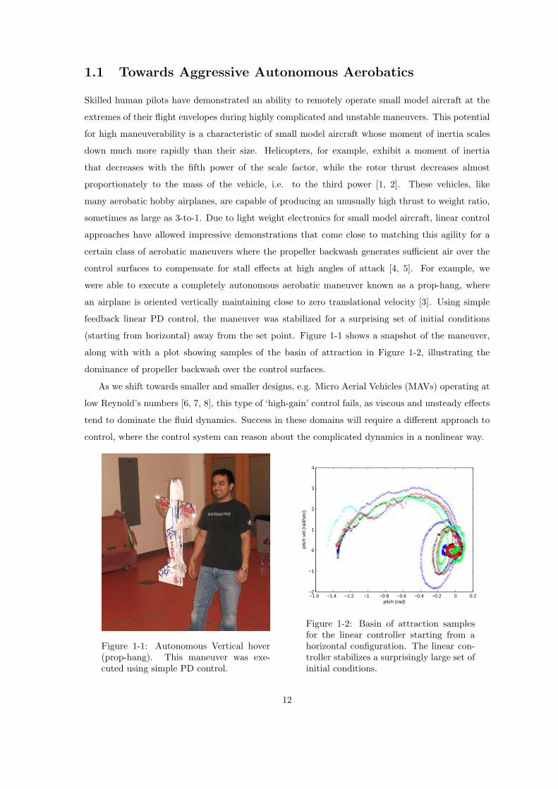
(starting from horizontal) away from the set point. Figure 1-1 shows a snapshot of the maneuver,
along with with a plot showing samples of the basin of attraction in Figure 1-2, illustrating the
dominance of propeller backwash over the control surfaces.
As we shift towards smaller and smaller designs, e.g. Micro Aerial Vehicles (MAVs) operating at
low Reynold’s numbers [6, 7, 8], this type of ‘high-gain’ control fails, as viscous and unsteady effects
tend to dominate the fluid dynamics. Success in these domains will require a different approach to
control, where the control system can reason about the complicated dynamics in a nonlinear way.
Figure 1-1: Autonomous Vertical hover(prop-hang). This maneuver was exe-cuted using simple PD control.
−1.6 −1.4 −1.2 −1 −0.8 −0.6 −0.4 −0.2 0 0.2−2
−1
0
1
2
3
4
pitch (rad)
pitc
h ve
l (ra
d/se
c)
Figure 1-2: Basin of attraction samplesfor the linear controller starting from ahorizontal configuration. The linear con-troller stabilizes a surprisingly large set ofinitial conditions.
12
1.2 Contributions and Organization
The contributions of this thesis includes results and methodologies for identifying an aerodynamic
model of a perching glider at very high angles of attack. This model is used as a basis for investigating
the control problem for a perching maneuver using an optimal control framework, and initial success
of a gradient following algorithm is shown on a simulated model of our glider.
The thesis is organized as follows: Chapter 2 introduces the general framework for the optimal
control problem along with a detailed derivation of the policy gradient algorithm used in Chapter
5. Chapter 3 introduces the general problem of aerobatic control and presents a literature review
highlighting relevant and related work. Chapter 4 describes in detail the requirements of our perching
task, our glider design, and experimental setup, in addition to presenting our methodology and
results for identifying an aerodynamic model at high angles of attack. Chapter 5 then describes
the results of applying the policy gradient algorithm of section 2.1. In particular, we show that a
compact parameterization of the task yields initial success using our dynamic simulation. Chapter
6 concludes with a discussion of our results and future work.
13
14
Chapter 2
The Optimal Control Approach
Many control problems in engineering are formulated in terms of an optimal control problem (e.g.
[11]), where the ultimate goal is to minimize some measure of cost on performance. In optimal
control, this cost metric is a scalar function of the state trajectory, the actions taken over that
trajectory, and possibly time.
Consider a discrete time dynamical system of the form:
xn+1 = f(xn,un) (2.1)
where xn represents the state of the system at time n and un represents the corresponding control
inputs. A value function represents the total cost incurred during the execution of a task when
starting at a given state x at a given instant in time
Jπ(x, n) = h(xN ) +N−1∑m=n
g(xm,um|xn = x,um = π(xm)) (2.2)
where the (deterministic policy) π(x) and the instantaneous cost g are both independent of time,
h represents a terminal cost, and N is the time horizon over which the task is executed. In this
thesis, we consider a time horizon that is policy dependent, which makes some algorithms more
easily applicable than others (see the following sections). Eq.(2.2) can be written recursively as
The optimal value function gives the optimal cost to go from any given state and is
J∗(x, N) = h(x) (2.5)
J∗(x, n) = argminu
[g(x,u) + J∗(f(x,u), n + 1)] (2.6)
The optimal policy is the one that minimizes the value function from any given state and is
π∗(x, n) = argminu
[g(xn,u) + J∗(f(xn,u), n + 1)] (2.7)
Unfortunately in robotics there exists very few examples that lend themselves to closed form
solutions for the optimal policy, in which case a computational approximation of the solution is used
instead. The following sections describe the different computational approaches used in this thesis.
2.1 Policy Gradient
Policy gradient algorithms are a class of reinforcement algorithms that search directly in the space
of policies vs. computing an exhaustive state space search for an optimal feedback policy, e.g.
in dynamic programming or value iteration [12]. They are typically subject to local minima and
smoothness constraints. The policy is typically parameterized by a vector w and is generally written
as un = πw(xn, n). The parameterization typically includes the user’s domain knowledge of the
control problem to restrict the solution to a particular class of policies. The goal in policy gradient
algorithms is to perform gradient descent on the policy parameters by computing the gradient of
the cost w.r.t. the parameterization vector and take small steps along this gradient to the local
optimum. Weight perturbation (a flavor of the well known REINFORCE algorithms [13]) provides
a simple algorithm for computing these policy gradients. Although true gradient descent using the
backpropogation through time algorithm [14], for example, would be more efficient, it requires an
explicit representation of the cost and plant gradients, which may be difficult to compute for policy
dependent time horizons (see section 5.1).
The simple idea in weight perturbation is to run a trial once with the original parameter vector
w, and then run a second trial with the parameter vector perturbed by some small random noise
vector. This will allow one to evaluate a change in the cost function with respect to changes in the
policy parameters. Given a general cost function (independent of time)
J(w,x0) =∞∑
n=0
g(xn, πw(xn)) (2.8)
The goal is to find an update of the form w = w + ∆w, where ∆w represents the change to the
16
parameters. If we choose an update such that the dot product
− ∂J
∂w·∆w > 0 (2.9)
then we can assure that the update will always be within 90◦ of the true gradient. Using a first
order Taylor expansion, the perturbed cost can be written as
J(w + ε) ≈ J(w) +∂J
∂wε , (2.10)
where ε is a random vector drawn from a zero-mean distribution. Consider the update
∆w = −η[J(w + ε)− J(w)]ε (2.11)
Using our Taylor expansion, we have
− ∂J
∂w·∆w = η
∂J
wε[J(w + ε)− J(w)] ≈ η
(∂J
wε
)2
> 0 , (2.12)
which satisfies Eq. 2.9. Note that the update requires evaluating the cost twice per update. One way
around this is to replace our baseline value J(w) with an estimate J(w) computed from previous
trials. More generally, however, we can replace our baseline with any estimator uncorrelated with
ε. The expected value of the update using a general baseline estimator b would then be
E[∆w] = −ηE
[[J(w + ε)− b]ε
](2.13)
≈ −ηE
[[J(w) +
∂J
∂wε− b]ε
](2.14)
= −ηE[J(w)− b]E[ε]− ηE[εεT ]∂J
∂w
T
(2.15)
= −ηE[εεT ]∂J
∂w
T
, (2.16)
where we used the fact that (J(w) − b) and ε are uncorrelated and E[ε] = 0. To assure that the
expected value of the update is in the direction of the true gradient we need
E{∆w} ∝ − ∂J
∂w(2.17)
which translates to having E[εεT ] ∝ I in 2.16. One way to achieve this is to choose each εi from a
normal distribution with mean 0 and variance σ2, such that E{εiεj} = 0 for i 6= j and E{εiεj} = σ2
17
otherwise. This gives us the standard weight perturbation update
∆w = − η
σ2[J(w + ε)− b]ε (2.18)
Even for an arbitrary baseline b, the expected value of the update will be in the direction of the
true gradient. In practice, using a good estimator for the baseline can dramatically improve learning
performance by reducing the variance of the updates.
Although this algorithm is simple to understand and implement, it requires the cost function
to be smooth with respect to the parameter vector w and is subject to local optimum. However,
weight perturbation is a great way to circumvent the curse of dimensionality as it (or any other policy
gradient algorithm) depends only on the specific parameterization of the policy and is independent
of the number of states in the system.
18
Chapter 3
Optimal Control for Aerobatic
Flight
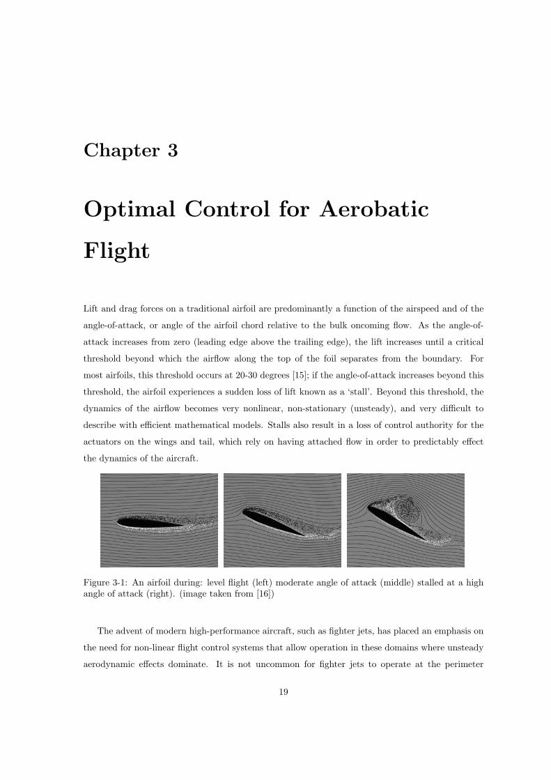
Lift and drag forces on a traditional airfoil are predominantly a function of the airspeed and of the
angle-of-attack, or angle of the airfoil chord relative to the bulk oncoming flow. As the angle-of-
attack increases from zero (leading edge above the trailing edge), the lift increases until a critical
threshold beyond which the airflow along the top of the foil separates from the boundary. For
most airfoils, this threshold occurs at 20-30 degrees [15]; if the angle-of-attack increases beyond this
threshold, the airfoil experiences a sudden loss of lift known as a ‘stall’. Beyond this threshold, the
dynamics of the airflow becomes very nonlinear, non-stationary (unsteady), and very difficult to
describe with efficient mathematical models. Stalls also result in a loss of control authority for the
actuators on the wings and tail, which rely on having attached flow in order to predictably effect
the dynamics of the aircraft.
Figure 3-1: An airfoil during: level flight (left) moderate angle of attack (middle) stalled at a highangle of attack (right). (image taken from [16])
The advent of modern high-performance aircraft, such as fighter jets, has placed an emphasis on
the need for non-linear flight control systems that allow operation in these domains where unsteady
aerodynamic effects dominate. It is not uncommon for fighter jets to operate at the perimeter
19
of their flight envelope during evasive maneuvers. These maneuvers are characterized by threats
of aerodynamic stall and other unsteady effects which could result in a dramatic loss of lift, such
as vortex bursting in low aspect ratio wings (e.g. delta wings). Conventional autopilot control
systems, however, are restricted to a much smaller flight-envelope, typically constrained to operate
between 0 and 15 degrees in angle-of-attack, where the flow around the wing stays attached and the
dynamics of the plane are nicely approximated by piecewise-linear models. Under these well behaved
conditions, aerodynamic forces and moments are approximated by linear terms in their Taylor Series
expansions, which lead to the well known stability derivative models [17]. It is important to note
that conventional stability and control derivative models along with standard force and moment
coefficient data alone fail to capture the internal state of the surrounding flow, which may contain
critical information about the future behavior of the aircraft. When applied in fighter jets at the
perimeter of their flight envelope, state-of-the-art fly-by-wire control systems have the potential of
experiencing a control ‘departure’ where the automated controller looses the ability to maintain
control of the aircraft. This can result in the aircraft entering a falling-leaf departure mode and,
depending on the severity of the situation, the pilot working with the control system may not always
be able to recover.
Due to these constraints imposed by state-of-the-art control technology, there has been very little
work on perching maneuvers for an aircraft. Recent results in reinforcement learning applied to robot
control having similarly complicated dynamics [18, 19], make this approach a strong candidate for
solving similar types of problems in aerobatic flight control.
3.1 Previous Work
Over the last fifteen years, the aeronautics community has made an effort to characterize dynamic
flight conditions through novel approaches to wind-tunnel data collection and dynamic modeling.
In this effort, Goman and Khrabrov [20] made an important contribution in their analysis of flow
separation and vortical flows. Through analysis of unsteady effects and flow seperation, their work
resulted in closed form unsteady coefficient models. These extended models captured the dependence
of aerodynamic forces and moments on motion prehistory, which in essence introduced part of the
flow characteristics into the description of the state.
A similar effort has been put forth in designing nonlinear control laws for aircraft maneuvering
in near stall regimes. A common approach described in the aeronautics literature [21],[22],[23] is
feedback linearization, otherwise known as inverse dynamics control. These methods typically make
use of complete sets of coefficient and derivative tables for a wide range of flight conditions in order to
compute aerodynamic forces and moments. Underlying assumptions then allow the control designer
to partially feedback linearize the dynamics using the available control surfaces and thrust vectors,
20
where it is assumed that these inputs can arbitrarily affect roll, pitch, and yaw angular accelerations.
Cross-coupling effects must also be ignored, such as lift and side-force contributions from various
control surface deflections. As a result, this type of dynamic inversion will hold only for high enough
dynamic pressure conditions where control surface inputs requiring deflections beyond saturation
limits will not become a problem and hence keep the system controllable.
Unmanned aerial vehicle (UAV) researchers have faced similar challenges in developing agile
autopilots for small-scale hobby aircraft. One thing to note, however, is that small UAVs have the
potential of completely overpowering part of the natural dynamics of the aircraft by employing an
extremely high thrust to weight ratio. However, even with this advantage, present day autopilots are
far from matching the maneuvering skills of a human UAV pilot. Although large motors allow almost
arbitrary corrections in certain directions, the system is still underactuated, making the problem
part of a larger class of problems where control and natural dynamics are intimately related and not
properly addressed by classical control methods.
Agile maneuvering for fixed-wing UAVs was presented in reference [24]. The work proposed an
approximate inverse dynamics model for agile maneuvering where the resultant control system was
tested in simulation. However, the maneuver performed was slow and well behaved, not representa-
tive of human piloted aerobatics. Work in [4] and [5] proposes a linear control system for performing
an autonomous prop-hang, similar to the work in [3]. An autopilot capable of a variety of aerobatic
maneuvers is proposed in [25]. However, video footage shows that the time scale for performing a
given maneuver is much larger than that of a human pilot [26].
The most notable work in autonomous UAV aerobatics has been on helicopters. Feron et al. were
one of the first to achieve autonomous aerobatic flight with a hobby helicopter [27], [31]. In this work
an analytical dynamic model was derived from basic principles and force coefficients were measured
through flight experiments. Noting successful results from Raibert[32] and Pratt[33], their control
system used an intuitive control approach where state machines were used based on human pilot
control data. For example, the controller encoded the observation that the collective command used
by the human pilot during maneuvers was roughly proportional to the cosine of the angle between
the vertical and z-axis. Through use of piecewise linear commands with specified switching times,
the authors were able to perform various maneuvers. Feron’s later work added feedback through
tight angular rate controllers on the pilot’s reference trajectory [34],[35].
Work by Bagnell [36] describe a unique approach to helicopter control, namely a computational
optimal control method, similar to the methods used in this thesis, known as reinforcement learning.
The authors presented a control policy search algorithm for stabilizing slow moving trajectories.
Later work by Ng et al. [37], [18] used a similar approach for aerobatic helicopter control. The
authors first fit a stochastic nonlinear model from pilot data, i.e. a model predicting either next
state or accelerations as a function of current state and control inputs. Next, a human pilot flight
21
trajectory for a desired aerobatic maneuver was used as the baseline for an offline control policy
search algorithm. Using this approach, an autonomous helicopter achieved stable inverted hover in
addition to a few aerobatic maneuvers at slow speeds. We note that (with the exception of inverted
hovering) Ng’s and Feron’s aerobatic control systems focused on stabilizing either a human pilot’s
trajectories or a state machine inspired by these trajectories. More recent work by Feron et al [40]
presents a control architecture for helicopters landing at unusual attitudes. They use a hand designed
state-machine to execute a perching maneuver that eventually lands on a large velcro launch pad.
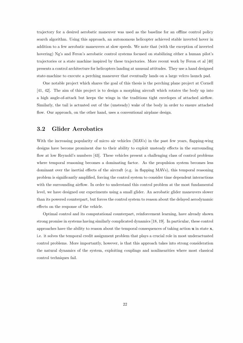
One notable project which shares the goal of this thesis is the perching plane project at Cornell
[41, 42]. The aim of this project is to design a morphing aircraft which rotates the body up into
a high angle-of-attack but keeps the wings in the traditions tight envelopes of attached airflow.
Similarly, the tail is actuated out of the (unsteady) wake of the body in order to ensure attached
flow. Our approach, on the other hand, uses a conventional airplane design.
3.2 Glider Aerobatics
With the increasing popularity of micro air vehicles (MAVs) in the past few years, flapping-wing
designs have become prominent due to their ability to exploit unsteady effects in the surrounding
flow at low Reynold’s numbers [43]. These vehicles present a challenging class of control problems
where temporal reasoning becomes a dominating factor. As the propulsion system becomes less
dominant over the inertial effects of the aircraft (e.g. in flapping MAVs), this temporal reasoning
problem is significantly amplified, forcing the control system to consider time dependent interactions
with the surrounding airflow. In order to understand this control problem at the most fundamental
level, we have designed our experiments using a small glider. An aerobatic glider maneuvers slower
than its powered counterpart, but forces the control system to reason about the delayed aerodynamic
effects on the response of the vehicle.
Optimal control and its computational counterpart, reinforcement learning, have already shown
strong promise in systems having similarly complicated dynamics [18, 19]. In particular, these control
approaches have the ability to reason about the temporal consequences of taking action u in state x,
i.e. it solves the temporal credit assignment problem that plays a crucial role in most underactuated
control problems. More importantly, however, is that this approach takes into strong consideration
the natural dynamics of the system, exploiting couplings and nonlinearities where most classical
control techniques fail.
22
Chapter 4
Perching with Fixed Wings
4.1 Problem Description
Perching is representative of any dynamic aerobatic maneuver that requires an agile and robust
control system with the capability of planning well into the future. The problem is described as
follows: A glider is launched 3.5m away from a perch at approximately 6m/s. What control policy
must the elevator follow in order to make a point landing on the perch with negligible velocity in a
fraction of a second? There are a number of implications that follow from executing such a maneuver:
1) the only way to induce such a dramatic drop in speed in such a short period of time is to orient
the aircraft to be almost perpendicular to the direction of travel, making use of the tremendous drag
generated by stalling the wings 2) the control system must reason about the dynamics well into the
future, before loosing all control authority as it approaches the perch 3) the control system must be
able to react to disturbances during the execution of the maneuver in real-time.
Instead of redesigning our aircraft in order to make traditional, linear control solutions effective,
we will start by designing an advanced control system for a conventional fixed-wing aircraft. In
the spirit of the Wright Brothers, whose eventual success in powered flight came from their deep
practical understanding of unpowered gliders, the experiments presented here are based on a small
unpropelled glider with a single actuator at the elevator launched in a controlled laboratory setting.
These machines are capable of perching, so long as the feedback system is capable of reasoning about
the complicated dynamics and intermittent loss of control authority on the control surfaces. We use
an optimal control framework whose properties are well known to handle temporal credit assignment
problems (i.e. reason about the consequences of an action well into the future). Moreover, this
framework gives us the tools for designing a full-state feedback control system, capable of responding
to disturbances in real time.
23
4.2 Indoor experimental setup
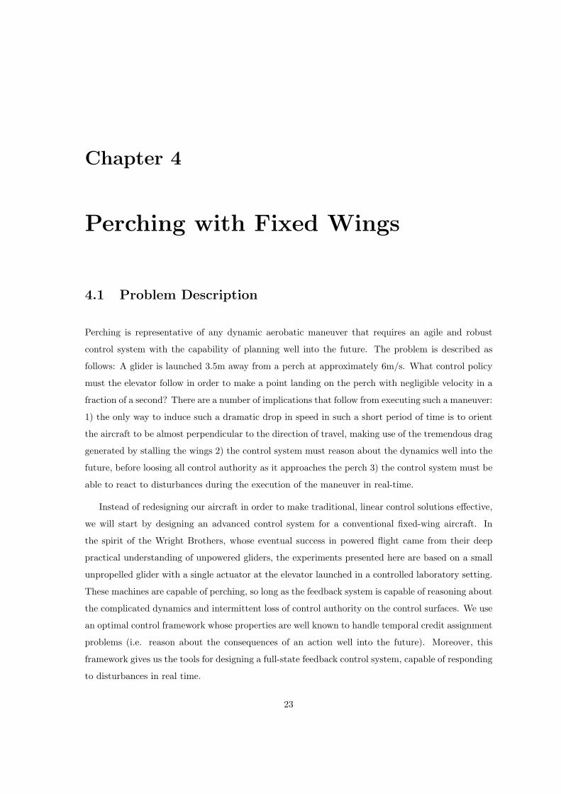
Figure 4-1: Vicon Motion Capture Environment. The Vicon motion capture setup makes use of 16infrared cameras to track small reflective markers along the body and control surface of the glider.These marker positions allow the system to reconstruct the position and orientation of the gliderwith high accuracy.
The task of landing on a perch is potentially filled with many rich and interesting subproblems
that require careful consideration in an integrated control system. Localizing (or even identifying)
a perch with noisy sensors in a natural gusty outdoor environment is itself a challenging task. In
order to study the core motor control problem, we have designed an indoor experimental facil-
ity which mitigates many of the complications including sensing, computation, and repeatability.
Our facility is equipped with a Vicon MX motion capture system consisting of 16 cameras, which
provides real-time sub-millimeter tracking of the vehicle and its control surface deflections (Figure
4-4 right), as well as the perch location. The basic setup is cartooned in Figure 4-1. Our indoor
setup has a capture volume of approximately 27m3 with hardware communicating new state in-
formation at approximately 120 frames per second, with 116ms total loop delay (including ground
station communication). This indoor flight environment providing off-board sensing, computation,
and control has proven to be an extremely effective experimental paradigm. In addition to still air
experiments, this environment allows us to consider artificially generated atmospheric disturbances
and flow visualizations in the future.
24
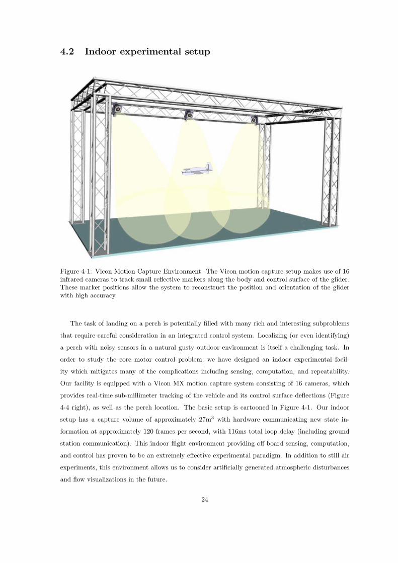
Figure 4-2: Cartoon of a feasible perching trajectory for a fixed-wing glider. This trajectory wasactually taken from the flight data described in the preliminary results section.
Our vehicle is launched into the motion capture environment from a small custom launching
device at speeds of approximately 6m/s and at Reynolds numbers ranging from 14,000-53,000 over
the entire perching trajectory. Once the motion capture system locks onto the glider, a ground-
station obtains real-time tracking information, implements the feedback policy, then sends commands
back to the vehicle over a standard radio-link interface. The task of the feedback loop is to bring
the vehicle to rest at the known perch location, which is approximately 3.5m from the location at
which the motion capture cameras lock onto the vehicle. The vehicle grabs the perch with a passive
mechanical one-way latch mounted just below the center of mass. The basic maneuver is cartooned
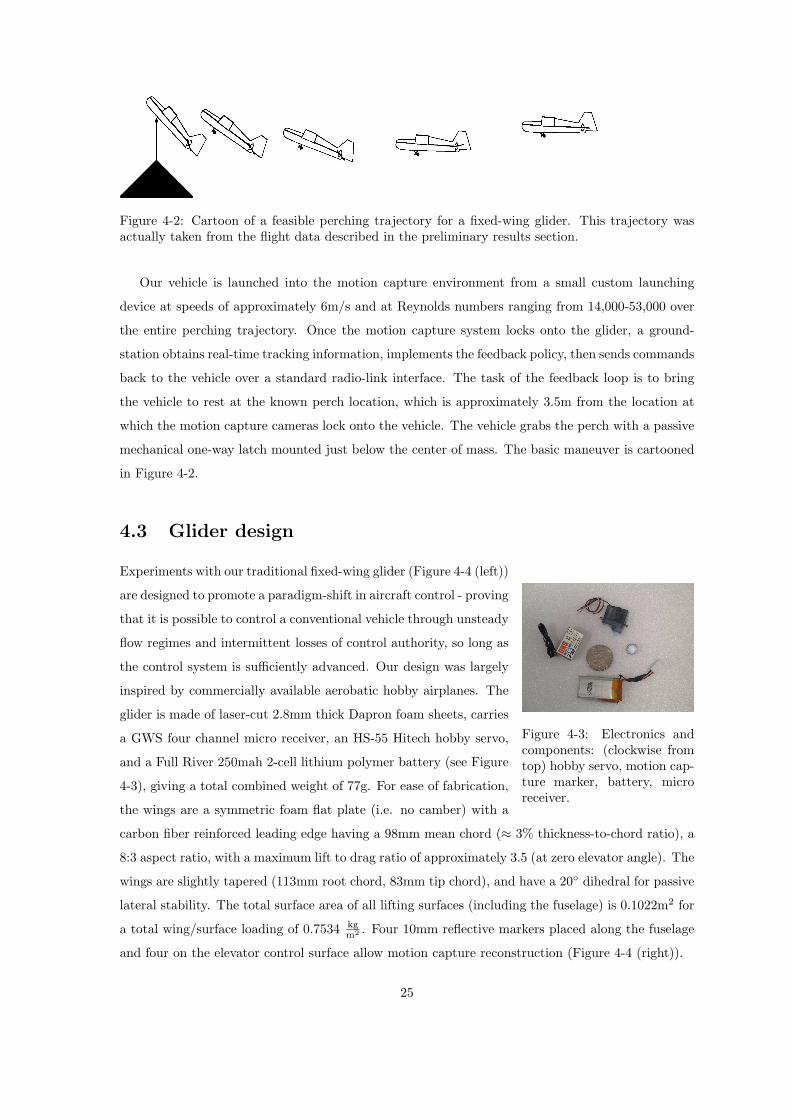
Experiments with our traditional fixed-wing glider (Figure 4-4 (left))
are designed to promote a paradigm-shift in aircraft control - proving
that it is possible to control a conventional vehicle through unsteady
flow regimes and intermittent losses of control authority, so long as
the control system is sufficiently advanced. Our design was largely
inspired by commercially available aerobatic hobby airplanes. The
glider is made of laser-cut 2.8mm thick Dapron foam sheets, carries
a GWS four channel micro receiver, an HS-55 Hitech hobby servo,
and a Full River 250mah 2-cell lithium polymer battery (see Figure
4-3), giving a total combined weight of 77g. For ease of fabrication,
the wings are a symmetric foam flat plate (i.e. no camber) with a
carbon fiber reinforced leading edge having a 98mm mean chord (≈ 3% thickness-to-chord ratio), a
8:3 aspect ratio, with a maximum lift to drag ratio of approximately 3.5 (at zero elevator angle). The
wings are slightly tapered (113mm root chord, 83mm tip chord), and have a 20◦ dihedral for passive
lateral stability. The total surface area of all lifting surfaces (including the fuselage) is 0.1022m2 for
a total wing/surface loading of 0.7534 kgm2 . Four 10mm reflective markers placed along the fuselage
and four on the elevator control surface allow motion capture reconstruction (Figure 4-4 (right)).
25
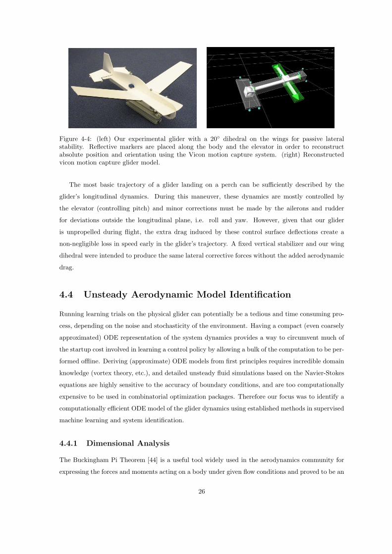
Figure 4-4: (left) Our experimental glider with a 20◦ dihedral on the wings for passive lateralstability. Reflective markers are placed along the body and the elevator in order to reconstructabsolute position and orientation using the Vicon motion capture system. (right) Reconstructedvicon motion capture glider model.
The most basic trajectory of a glider landing on a perch can be sufficiently described by the
glider’s longitudinal dynamics. During this maneuver, these dynamics are mostly controlled by
the elevator (controlling pitch) and minor corrections must be made by the ailerons and rudder
for deviations outside the longitudinal plane, i.e. roll and yaw. However, given that our glider
is unpropelled during flight, the extra drag induced by these control surface deflections create a
non-negligible loss in speed early in the glider’s trajectory. A fixed vertical stabilizer and our wing
dihedral were intended to produce the same lateral corrective forces without the added aerodynamic
drag.
4.4 Unsteady Aerodynamic Model Identification
Running learning trials on the physical glider can potentially be a tedious and time consuming pro-
cess, depending on the noise and stochasticity of the environment. Having a compact (even coarsely
approximated) ODE representation of the system dynamics provides a way to circumvent much of
the startup cost involved in learning a control policy by allowing a bulk of the computation to be per-
formed offline. Deriving (approximate) ODE models from first principles requires incredible domain
knowledge (vortex theory, etc.), and detailed unsteady fluid simulations based on the Navier-Stokes
equations are highly sensitive to the accuracy of boundary conditions, and are too computationally
expensive to be used in combinatorial optimization packages. Therefore our focus was to identify a
computationally efficient ODE model of the glider dynamics using established methods in supervised
machine learning and system identification.
4.4.1 Dimensional Analysis
The Buckingham Pi Theorem [44] is a useful tool widely used in the aerodynamics community for
expressing the forces and moments acting on a body under given flow conditions and proved to be an
26
important source of domain knowledge for identifying the aerodynamic model. Using this approach,
here we include a simplified derivation (see [45]) of the equations used to parameterize our model.
For a fixed angle of attack (and a fixed body shape) we assume that the total force F is a function
of the five variables shown in Table 4.1.
Physical Quantity Description DimensionsF force ml/t2
V∞ velocity l/tρ∞ density m/l3
S surface l2
a∞ free stream speed of sound l/tµ∞ viscosity m/lt
Table 4.1: Dimensional Parameters
In Table 4.1, the subscript ∞ denotes a free stream value. We can then assume a functional form
for the aerodynamic force as:
F = kV a∞ρb
∞Sdae∞µf
∞ (4.1)
where k is some dimensionless constant. Equating dimensions we get:
ml
t2=
(l
t
)a (m
l3
)b
(l2)d
(l
t
)e (m
lt
)f
(4.2)
Equating exponents for like dimensions gives us the result:
F = k(V∞)2−e−fρ1−f∞ S1−f/2ae
∞µf∞ (4.3)
= kρ∞V 2∞S
(a∞V∞
)e
︸ ︷︷ ︸Mach no.−1
(µ∞
ρ∞V∞S1/2
)f
︸ ︷︷ ︸Re−1
(4.4)
We now throw all source of uncertainty into a single force coefficient Cf and can write
Cf = 2k
(1
M∞
)e (1
Re
)f
(4.5)
F =12ρ∞V 2
∞SCf (4.6)
where M∞ is the free stream mach number and Re is the Reynolds Number. We again note that this
holds for a fixed angle-of-attack, which therefore makes Cf a function of angle of attack in addition
to the variables in 4.5.
27
4.4.2 Approximating Force and Moment Coefficients
Contrary to conventional wind tunnel techniques used for steady aerodynamic model identifica-
tion, we trained a (coarsely approximated) unsteady aerodynamic model using supervised learning
methods applied to real flight data. The representation of our dynamic model exploits standard
relationships between aerodynamic forces/moments and their corresponding non-dimensionalized
coefficients, which allows the model to generalize well beyond the limits of our data. The identified
model approximates lift, drag, and moment coefficients as functions of angle of attack and elevator
deflection angle.
We logged approximately 240 trials of real flight data over unsteady regimes of the flight envelope,
including stall and post-stall configurations, in our motion capture environment. Our trials swept
a representative set of flight trajectories for the perching maneuver and the data was processed
and used to compute instantaneous forces and moments using the standard equations F = ma and
τ = Iα, where F represents the linear force vector, m is mass, a is the linear acceleration vector, I is
the inertia about the glider’s center of gravity, and α is the rotational acceleration. The force vector
was decomposed into lift and drag components and was then used to compute the instantaneous
force and moment coefficients as:
CL =2FL
ρV 2SCD =
2FD
ρV 2SCM =
2M
ρV 2Sc(4.7)
where CL, CD, and CM represent lift,drag, and moment coefficients, respectively. The collected co-
efficient data was used to model the (averaged) unsteady aerodynamic force and moment coefficients
as functions of angle of attack and elevator angle using a linear barycentric function approximator
[46] with nonlinear features of the inputs.
C = WΦ(X) (4.8)
where C is the coefficient data, W represent the unknown parameter matrix, X is the input data
consisting of angle of attack and elevator angle, and Φ(X) represents the nonlinear features of the
input data. The parameter matrix was estimated using standard least squares ridge regression:
W = (ΦT Φ + λI)−1ΦT W (4.9)
where
W = argminW
tr[(C−WΦ)T (C−ΦW) + λWT W] (4.10)
where we used Φ as shorthand for Φ(X). Ridge regression shrinks the parameters by imposing
a penalty on their size, eliminating large parameter magnitudes in regions where data was sparse
28
−20 0 20 40 60 80 100 120 140 160−1.5
−1
−0.5
0
0.5
1
1.5
Angle of Attack
Cl
Glider DataFlat Plate Theory
−20 0 20 40 60 80 100 120 140 160−0.5
0
0.5
1
1.5
2
2.5
3
3.5
Angle of Attack
Cd
Glider DataFlat Plate Theory
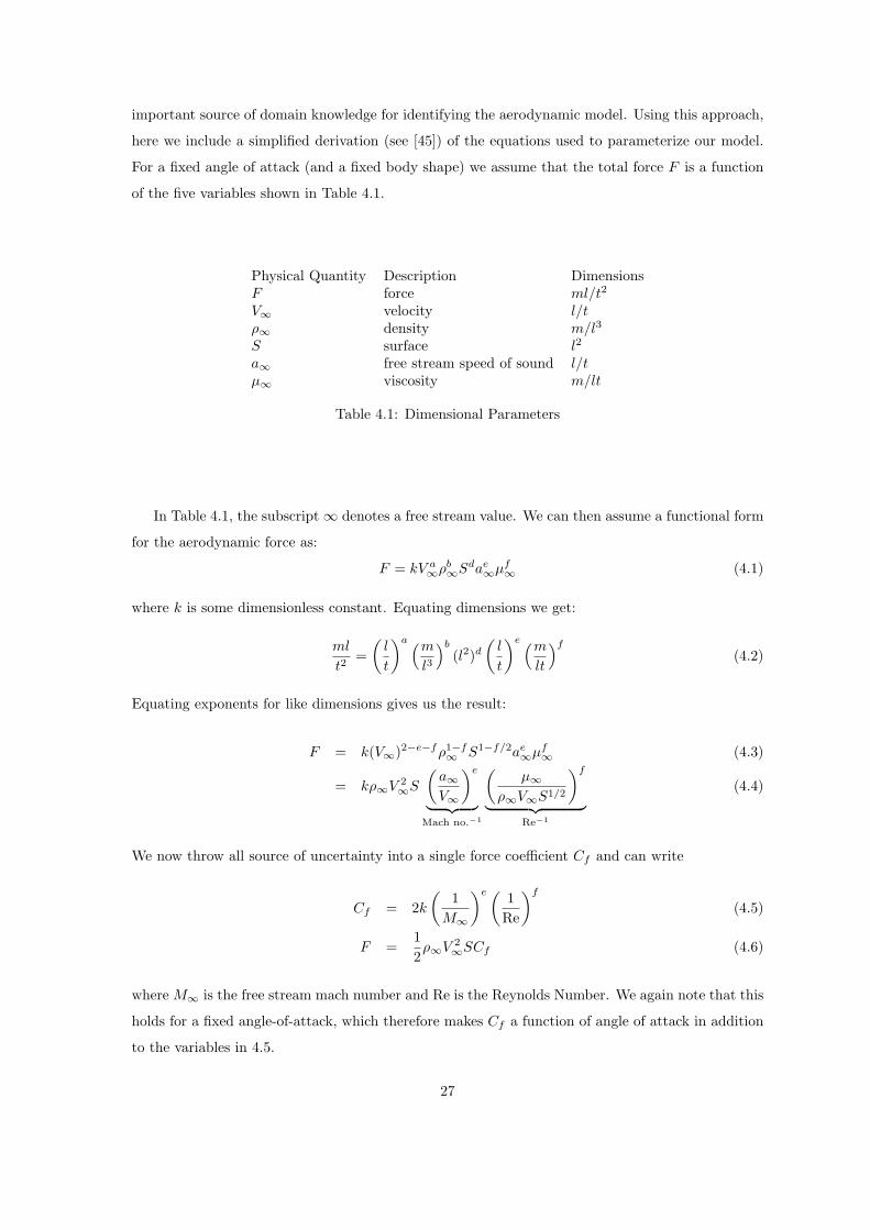
Figure 4-5: Scatter plots showing the general trend of the computed coefficients from flight data.Shown are lift and drag coefficients with their respective flat plate theory predictions.
−0.5 0 0.5 1 1.5 2 2.5 3 3.5−1.5
−1
−0.5
0
0.5
1
1.5
Cd
Cl
Glider DataFlat Plate Theory
Figure 4-6: Lift to Drag polar plots and its respective flat plate theory prediction.
(typically at the boundaries of the approximation). Our data was post-processed (down-sampled
at 30Hz) with a recursive outlier detection scheme that removed data points outside five standard
deviations of the current best fit. The model was re-fit until no outliers were found.
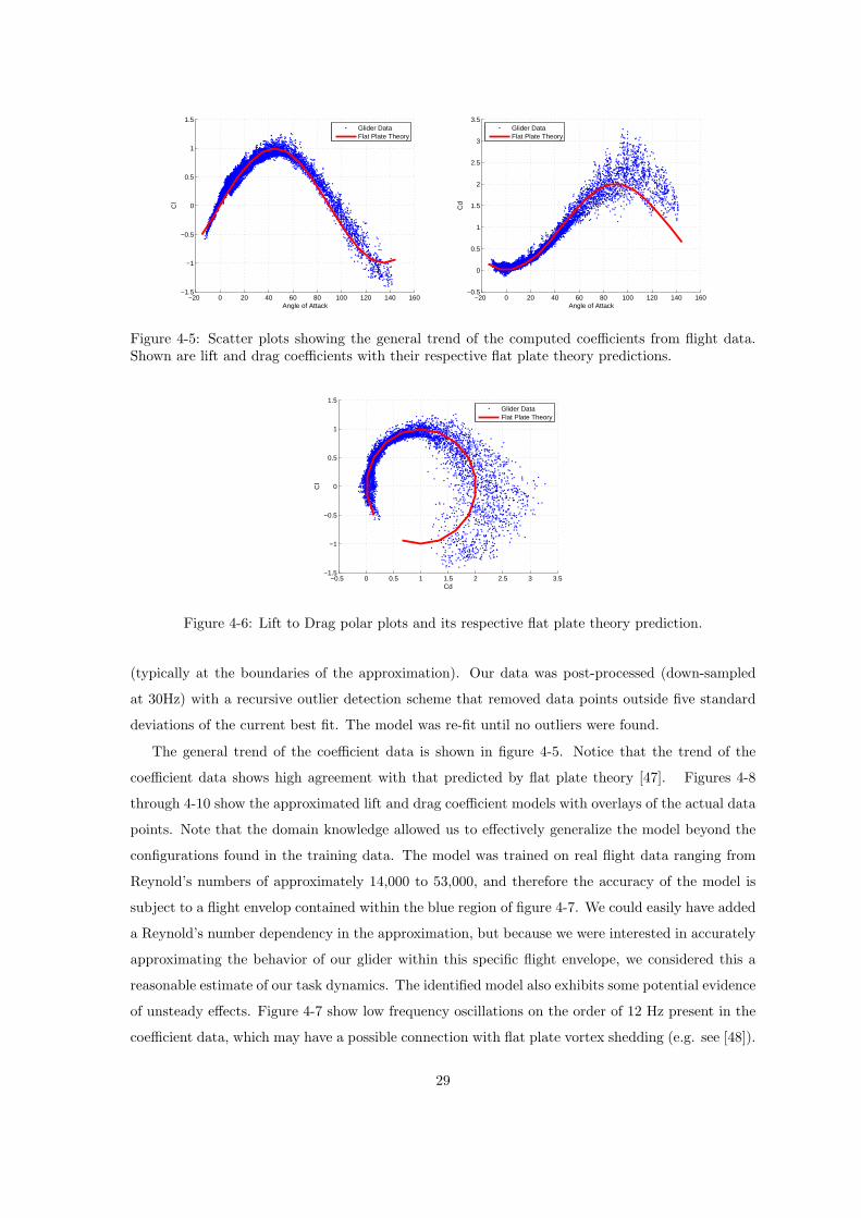
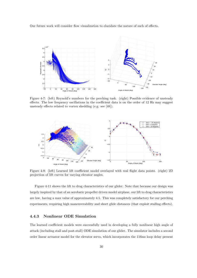
The general trend of the coefficient data is shown in figure 4-5. Notice that the trend of the
coefficient data shows high agreement with that predicted by flat plate theory [47]. Figures 4-8
through 4-10 show the approximated lift and drag coefficient models with overlays of the actual data
points. Note that the domain knowledge allowed us to effectively generalize the model beyond the
configurations found in the training data. The model was trained on real flight data ranging from
Reynold’s numbers of approximately 14,000 to 53,000, and therefore the accuracy of the model is
subject to a flight envelop contained within the blue region of figure 4-7. We could easily have added
a Reynold’s number dependency in the approximation, but because we were interested in accurately
approximating the behavior of our glider within this specific flight envelope, we considered this a
reasonable estimate of our task dynamics. The identified model also exhibits some potential evidence
of unsteady effects. Figure 4-7 show low frequency oscillations on the order of 12 Hz present in the
coefficient data, which may have a possible connection with flat plate vortex shedding (e.g. see [48]).
29
Our future work will consider flow visualization to elucidate the nature of such of effects.
−20 0 20 40 60 80 100 120 140 1601
1.5
2
2.5
3
3.5
4
4.5
5
5.5x 10
4
Angle of Attack (deg)
Rey
nold
’s N
umbe
r
−500
50100
150−40
−30
−20
−10
0
10
20
30
−2
−1
0
1
2
Elevator Angle (deg)
Angle of Attack (deg)
Cl
Figure 4-7: (left) Reynold’s numbers for the perching task. (right) Possible evidence of unsteadyeffects. The low frequency oscillations in the coefficient data is on the order of 12 Hz may suggestunsteady effects related to vortex shedding (e.g. see [48]).
Figure 4-8: (left) Learned lift coefficient model overlayed with real flight data points. (right) 2Dprojection of lift curves for varying elevator angles.
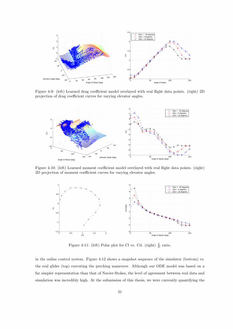
Figure 4-11 shows the lift to drag characteristics of our glider. Note that because our design was
largely inspired by that of an aerobatic propeller driven model airplane, our lift to drag characteristics
are low, having a max value of approximately 4.5. This was completely satisfactory for our perching
experiments, requiring high maneuverability and short glide distances (that exploit stalling effects).
4.4.3 Nonlinear ODE Simulation
The learned coefficient models were successfully used in developing a fully nonlinear high angle of
attack (including stall and post-stall) ODE simulation of our glider. The simulator includes a second
order linear actuator model for the elevator servo, which incorporates the 116ms loop delay present
Figure 4-9: (left) Learned drag coefficient model overlayed with real flight data points. (right) 2Dprojection of drag coefficient curves for varying elevator angles.
Figure 4-10: (left) Learned moment coefficient model overlayed with real flight data points. (right)2D projection of moment coefficient curves for varying elevator angles.
Figure 4-11: (left) Polar plot for Cl vs. Cd. (right) LD ratio.
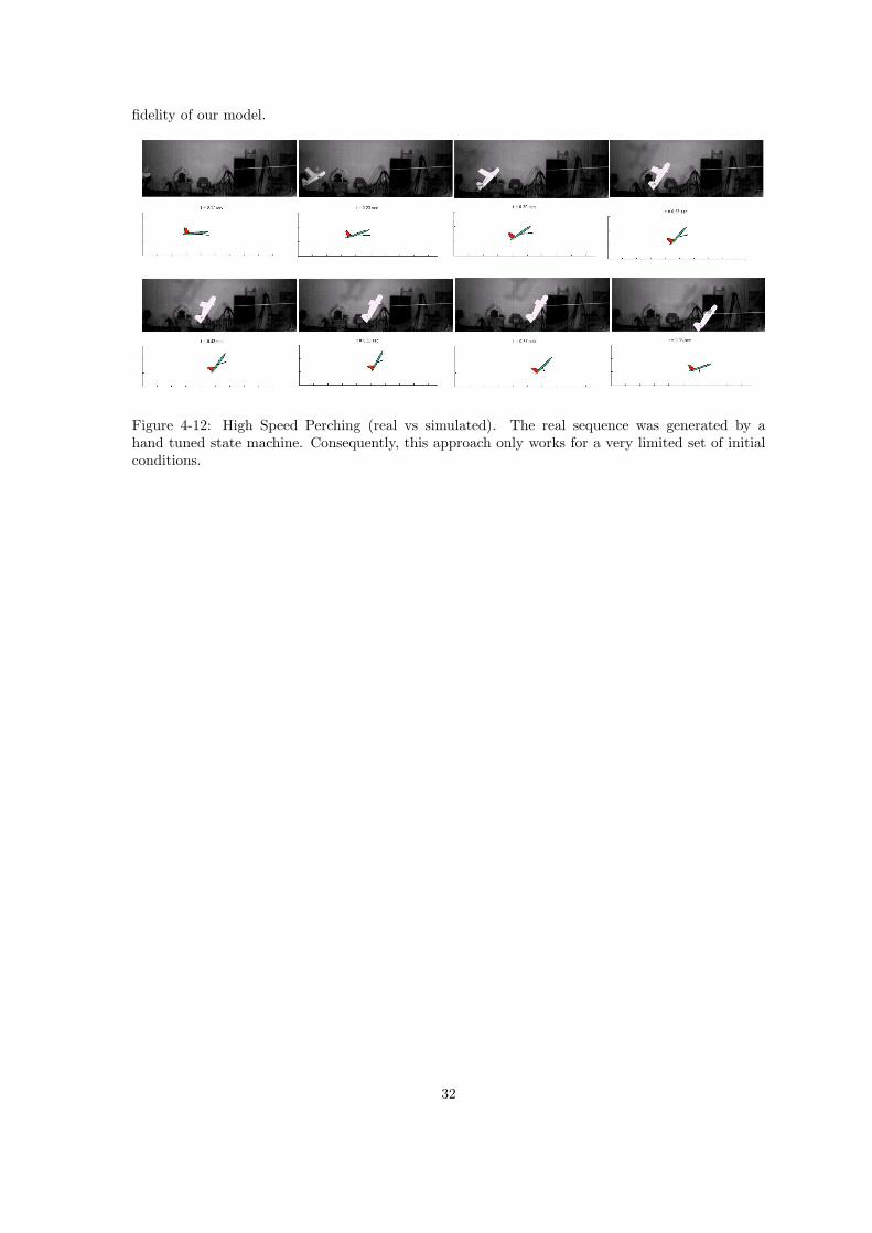
in the online control system. Figure 4-12 shows a snapshot sequence of the simulator (bottom) vs.
the real glider (top) executing the perching maneuver. Although our ODE model was based on a
far simpler representation than that of Navier-Stokes, the level of agreement between real data and
simulation was incredibly high. At the submission of this thesis, we were currently quantifying the
31
fidelity of our model.
Figure 4-12: High Speed Perching (real vs simulated). The real sequence was generated by ahand tuned state machine. Consequently, this approach only works for a very limited set of initialconditions.
32
Chapter 5
An Autopilot that Lands On a
Perch
For our simplified two dimensional problem we have an eight dimensional state vector and a one
dimensional action vector given by
x =[
y z θ ψ y z θ ψ]T
and u = elevator command (5.1)
where (y, z) are cartesian position coordinates w.r.t. the perch location, θ is the glider pitch angle
with respect to the floor, and ψ represents the elevator deflection angle w.r.t. the glider.
5.1 Acquiring a Direct Policy
Acquiring a policy directly has important advantages over complete state-space search methods.
In particular, direct policy search algorithms are independent of the dimensionality of the problem
and instead depend on the specific parameterization being used. The control approach described
here was inspired by a hand tuned state-machine controller that was used to execute the perching
maneuver. Figure 4-12 (bottom) shows the results of this state machine controller. However, this
controller works only from a very limited set of initial conditions. Our goal here was to broaden the
basin of attraction for the same parameterization using a policy gradient approach, based on the
algorithm described in section 2.1.
5.1.1 Optimizing Parameters by Weight Perturbation
If we assume that most of the variability in cost comes from the variability in initial launching
conditions then we can restrict our class of policies to those that map initial conditions to control
33
actions. Namely, we can have our policy output two parameters for a given initial condition which
define: 1) a coordinate defining a transition into a high angle of attack (this coordinate is distance
relative to the perch) and 2) the magnitude of this deflection in terms of elevator angle. The policy
is a nonlinear function Θ of the parameterization vector w and nonlinear features φ taken over the
set of initial conditions drawn from real trials.
πw(x,xic) = Θ
(x,
∑
i
wiφi(xic)
)(5.2)
where xic is an initial condition state vector. The parameterization gives us two control variables
as follows:
ydef
emag
= K
I +
tanh
(∑Ni=1 w1,iφi(xic)
)
tanh(∑N
i=1 w2,iφi(xic))
(5.3)
where ydef is the y coordinate that specifies the point at which to deflect the elevator (to cause a nose
up moment), emag is the magnitude of this elevator deflection, and K is a diagonal gain matrix. We
use an offset tanh function to make the control variables positive and smooth w.r.t. the parameter
vector w. The policy is then given by:
un = πw(xn,xic) = ξ(yn − ydef)emag︸ ︷︷ ︸Θ
(5.4)
where ξ is the Heaviside or unit step function given by
ξ(c) ={
0 c < 0
1 c ≥ 0(5.5)
A learning trial consists of launching the glider at the given initial condition (in simulation), executing
the current policy, and making a policy gradient update at the end of the trial, which happens when
the glider hits the floor. The cost-to-go is defined as
J(x, n) = minxm
[(xm − xdes)T Q(xm − xdes),m = n, . . . , N ] (5.6)
where xdes represents the desired state for a successful perch (where the perch coordinates are
assumed to be (y, z) = (0, 0)) and is chosen as xdes = [0 0 π4 NA 0 − 1 − 1 NA]. Here position is
given in meters, angles in radians, and NA indicates that the elevator state is not penalized. This
cost translates to penalizing at the ‘best’ point in the trajectory in terms of squared error. In practice
Q changes about z = 0, where we penalize states ending below the perch more so than those that
end above, essentially giving the cost a non-quadratic form. This introduces a slight discontinuity
34
into the cost function, but in practice it never presented a problem for the optimization process.
However, although Eq.(5.6) is intuitively simple to understand, it is not a conventional additive
cost function (e.g. Eq.(2.2)). Instead the total cost depends on the entire state trajectory and the
time horizon N varies and is dependent on the policy being followed (depending on the policy, the
glider will hit the floor at different times and ∂N/∂w 6= 0). This makes exact gradient calculations
a little more difficult (e.g. as needed by backpropogation through time [14]) and was one of our
motivations for using model-free weight perturbation. Using the weight perturbation algorithm (see
sec. 2.1) we were able to acquire a policy offline using our identified dynamic model. The set of
initial conditions seen from trial data was discretized into a five dimensional mesh over the five
state variables describing the initial condition of the launch xic = [z θ x z θ]T , the other three
state variables were assumed to be always known and invariant. The algorithm optimized the policy
parameters for every initial condition in the mesh (approximately 1024 points) using a distributed
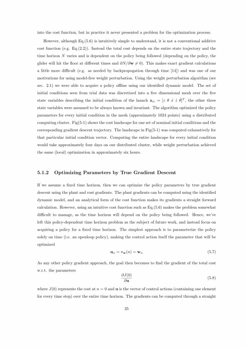
computing cluster. Fig(5-1) shows the cost landscape for one set of nominal initial conditions and the
corresponding gradient descent trajectory. The landscape in Fig(5-1) was computed exhaustively for
that particular initial condition vector. Computing the entire landscape for every initial condition
would take approximately four days on our distributed cluster, while weight perturbation achieved
the same (local) optimization in approximately six hours.
5.1.2 Optimizing Parameters by True Gradient Descent
If we assume a fixed time horizon, then we can optimize the policy parameters by true gradient
descent using the plant and cost gradients. The plant gradients can be computed using the identified
dynamic model, and an analytical form of the cost function makes its gradients a straight forward
calculation. However, using an intuitive cost function such as Eq.(5.6) makes the problem somewhat
difficult to manage, as the time horizon will depend on the policy being followed. Hence, we’ve
left this policy-dependent time horizon problem as the subject of future work, and instead focus on
acquiring a policy for a fixed time horizon. The simplest approach is to parameterize the policy
solely on time (i.e. an openloop policy), making the control action itself the parameter that will be
optimized
un = πw(n) = wn (5.7)
As any other policy gradient approach, the goal then becomes to find the gradient of the total cost
w.r.t. the parameters∂J(0)∂u
(5.8)
where J(0) represents the cost at n = 0 and u is the vector of control actions (containing one element
for every time step) over the entire time horizon. The gradients can be computed through a straight
35
Figure 5-1: Cost landscape for a given initial condition and the corresponding policy gradient tra-jectory(red)
forward calculation
∂J(0)∂uN−1
=∂J(N − 1)
∂uN−1=
∂g(xN−1, uN−1)∂uN−1
+∂g(xN )∂xN
∂xN
∂uN−1(5.9)
where we observe that the instantaneous cost g(xn, un) for n = 0, . . . , j − 1 does not depend on the
command uj . In a similar fashion, we can compute the other gradients and find the backward pass
recursion
∂J
∂uN−k=
∂gN−k
∂uN−k+
∂J
∂xN−k+1
∂fN−k
∂uN−k(5.10)
∂J
∂xN−k=
∂gN−k
∂xN−k+
∂J
∂xN−k+1
∂fN−k
∂xN−k(5.11)
This approach, commonly known as the backpropogation through time algorithm [14], plays out
a trajectory using the current policy, then makes a backward pass to compute the update to the
control parameters. Using this approach, we were able to obtain an openloop policy for the perching
task in simulation for a single initial conditon, and used those results as part of our basis for our
parameterization chosen in section 5.1. Another approach would be to generate a full state feedback
36
policy based on time as well as state using the backpropogation through time algorithm. This would
require a mesh over time and space that is rather large, requiring 8+ Ndt dimensions (8 state variables
and Ndt time steps), consequently bearing no advantage over methods such as dynamic programming.
Therefore, a more clever parameterization would be required and is the subject of future work.
37
38
Chapter 6
Conclusions and Future Work
Controlling a glider in unsteady airflow conditions provides a benchmark task for understanding
the basic principles of maneuverable flight. Studying gliding flight allows us to study the perching
problem at its core, stripping the problem down to its most fundamental level. Leveraging new
motion capture technology, we were able to identify a dynamic model within the flight envelop of
the perching task using methods in supervised learning and system identification. This has provided
not only a way to circumvent the high startup cost of online learning, but also invaluable task-specific
domain knowledge that will be useful as we move towards perching with flapping-wings. The next
step of this work will be to evaluate the results presented here on the real glider, where model-free
learning will close the gap between the controller optimized in simulation and the one that will
provide successful results on the real glider.
6.1 Outdoor Sensing and Control
Performing a perching maneuver in an outdoor setting would truly illustrate the high level of ro-
bust intelligence in any control solution. To this end, we have already designed and built a fully-
instrumented autonomous sail plane capable of carrying a 440g instrumentation payload, shown in
Figure 6-1. This sailplane has already shown the ability to fly completely under computer control.
The payload includes an on-board Pentium based PC104 computer running real-time Matlab, a
3DM-GX1 sensor package combining three 1200◦/sec angular rate gyros with three orthogonal DC
accelerometers and magnatometers, and an on-board Ethernet bridge providing Wi-Fi communica-
tion with a ground station. Our next step in our outdoor experiments will be to introduce a number
of sensors onto the aircraft in order to facilitate the detection of a perch and successful execution of
the point landing in spite of gusty wind conditions. The aircraft’s perch detection suite will incorpo-
rate differential GPS along with stereo vision (all processed on board) in combination with contact
sensors that will detect a successful landing. Local air flow sensors along the body and along the
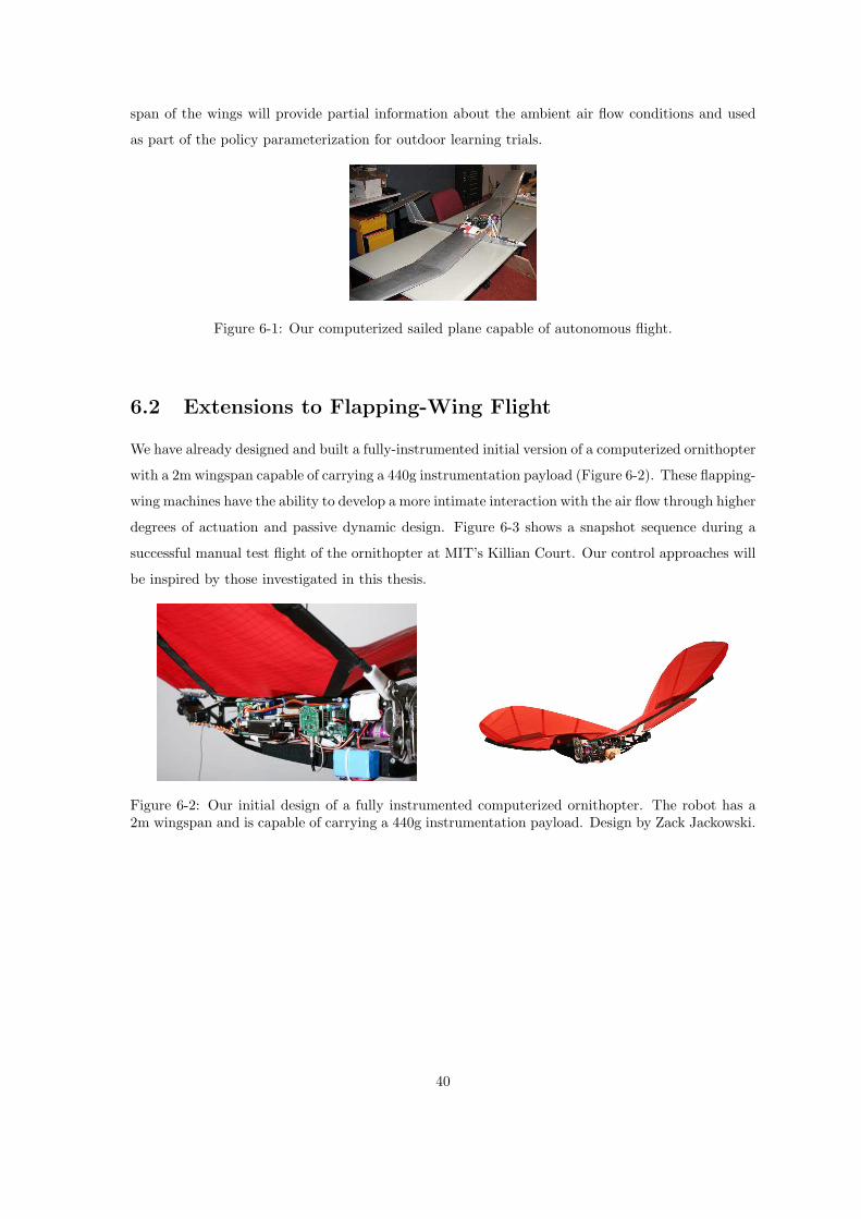
39
span of the wings will provide partial information about the ambient air flow conditions and used
as part of the policy parameterization for outdoor learning trials.
Figure 6-1: Our computerized sailed plane capable of autonomous flight.
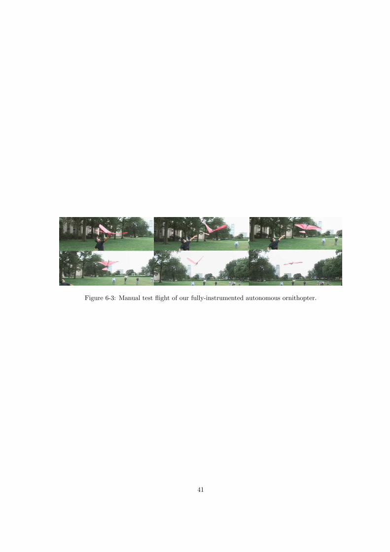
6.2 Extensions to Flapping-Wing Flight
We have already designed and built a fully-instrumented initial version of a computerized ornithopter
with a 2m wingspan capable of carrying a 440g instrumentation payload (Figure 6-2). These flapping-
wing machines have the ability to develop a more intimate interaction with the air flow through higher
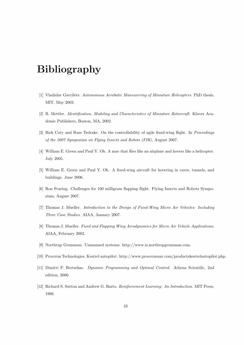
degrees of actuation and passive dynamic design. Figure 6-3 shows a snapshot sequence during a
successful manual test flight of the ornithopter at MIT’s Killian Court. Our control approaches will
be inspired by those investigated in this thesis.
Figure 6-2: Our initial design of a fully instrumented computerized ornithopter. The robot has a2m wingspan and is capable of carrying a 440g instrumentation payload. Design by Zack Jackowski.
40
Figure 6-3: Manual test flight of our fully-instrumented autonomous ornithopter.