T H E U N I V E R S I T Y O F E D I N B U R G H Performance analysis and optimisation of LAMMPS on XCmaster, HPCx and Blue Gene Geraldine McKenna August 23, 2007 MSc in High Performance Computing The University of Edinburgh Year of Presentation: 2007
Transcript
TH
E
U N I V E RS
I TY
OF
ED I N B U
RG
H
Performance analysis and optimisation of LAMMPS on XCmaster,HPCx and Blue Gene
Geraldine McKenna
August 23, 2007
MSc in High Performance Computing
The University of Edinburgh
Year of Presentation: 2007
Abstract
Rapid developments in laser technology over the last decade have enabled experimentalists to investigatethe dynamics of molecules in high intensity laser fields. Progress has been made theoretically to understandthe molecular dynamics involved, but, there remain a number of significant computational challenges. Themolecular system is computed by means of computer simulation codes running on massively parallel ma-chines. In order to obtain optimal performance from such codes, the efficiency and scalability of the code isa major contributing factor.
This project focuses on investigating the performance of LAMMPS molecular dynamics code (supportedby MPI implementation) on three different systems: XCmaster, HPCx and Blue Gene. The code has beensuccessfully ported to each of the systems and the speedup of LAMMPS is investigated on up to 1024processors on HPCx and Blue Gene and up to 16 processors on XCmaster. The code is found to scale wellto 1024 processors with a drop in speedup beyond 256 processors on the HPCx system. Reasons for thedifference in performance on each system are provided.
Profiling is used to identify the computationally expensive components of the code. Optimising these com-ponents is found to improve the serial performance of LAMMPS by up to 2% and the parallel performanceup to 18%. These figures depend on the benchmark used, the number of processors and the system on whichthe code is run. The impact of communication latency on the scalability of the code can be seen at largeprocessor counts.
The effects of simultaneous multithreading on the HPCx system are also investigated to determine if any per-formance improvement is obtainable. The LAMMPS code is benchmarked with and without SMT enabled.The performance is found to improve up to a factor of 2.28.
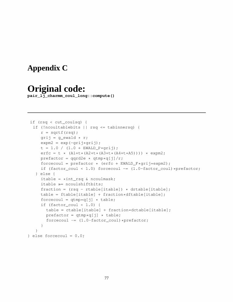
C Original code:pair_lj_charmm_coul_long::compute() 77
D Work plan 78
E Minutes of meetings 80
ii
List of Tables
3.1 Breakdown of the time spent in different sections of the code for the sodium montmorillonitebenchmark (500 timesteps) run on 8 processors on the XCmaster system. . . . . . . . . . . . 23
3.2 Breakdown of the time spent in different sections of the code for the sodium montmorillonitebenchmark (500 timesteps) run on 16 processors on the XCmaster system. . . . . . . . . . . 23
3.3 A summary of the different benchmarks used in the simulations. . . . . . . . . . . . . . . . . 263.4 Startup costs of the rhodopsin protein benchmark (32000 atoms) on the XCmaster system. . 373.5 Startup costs of the sodium montmorillonite benchmark (1033900 atoms) on the XCmaster
system. . . . . . . . . . . . . . . . . . . . . . . . . . . . . . . . . . . . . . . . . . . . . . . 373.6 Results obtained from running LAMMPS on the "32 processor" queue on the XCmaster system. 383.7 Comparison of the timings obtained for the sodium montmorillonite benchmark (1033900
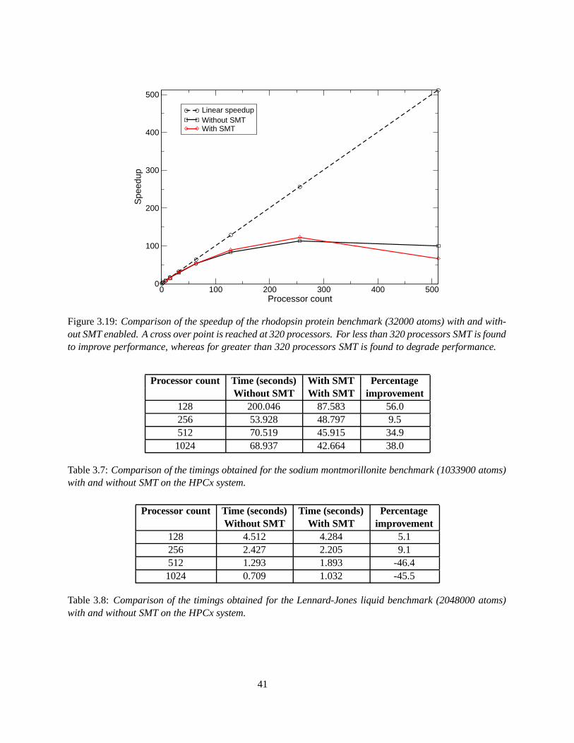
atoms) with and without SMT on the HPCx system. . . . . . . . . . . . . . . . . . . . . . . 413.8 Comparison of the timings obtained for the Lennard-Jones liquid benchmark (2048000
atoms) with and without SMT on the HPCx system. . . . . . . . . . . . . . . . . . . . . . . 41
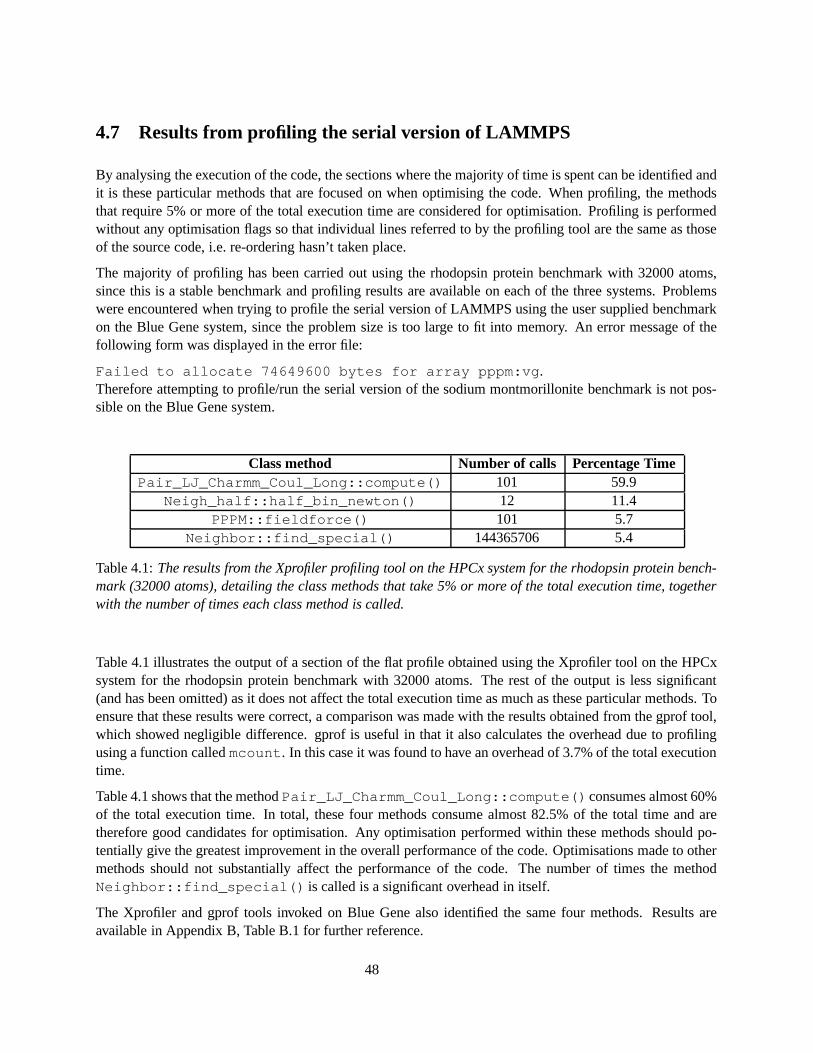
4.1 The results from the Xprofiler profiling tool on the HPCx system for the rhodopsin proteinbenchmark (32000 atoms), detailing the class methods that take 5% or more of the totalexecution time, together with the number of times each class method is called. . . . . . . . . 48
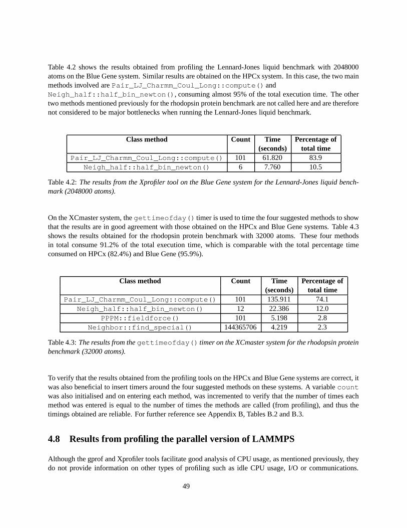
4.2 The results from the Xprofiler tool on the Blue Gene system for the Lennard-Jones liquidbenchmark (2048000 atoms). . . . . . . . . . . . . . . . . . . . . . . . . . . . . . . . . . . 49
4.3 The results from the gettimeofday() timer on the XCmaster system for the rhodopsinprotein benchmark (32000 atoms). . . . . . . . . . . . . . . . . . . . . . . . . . . . . . . . 49
4.4 Comparison of the amount of time spent in different MPI routines (obtained using the MPI-Trace profiling tool) for the rhodopsin protein benchmark (32000 atoms) run on 16 and 128processors on HPCx. . . . . . . . . . . . . . . . . . . . . . . . . . . . . . . . . . . . . . . 52
4.5 The overheads associated with using different profiling tools/timers on the XCmaster, HPCxand Blue Gene systems. . . . . . . . . . . . . . . . . . . . . . . . . . . . . . . . . . . . . . 56
6.1 Serial LAMMPS performance using the rhodopsin protein benchmark (32000 atoms) on theXCmaster, HPCx and Blue Gene systems. . . . . . . . . . . . . . . . . . . . . . . . . . . . 65
6.3 The results of the gettimeofday() timer on the XCmaster system after optimisation forthe rhodopsin protein (32000 atoms). . . . . . . . . . . . . . . . . . . . . . . . . . . . . . . 66
6.4 The rhodopsin protein benchmark with 32000 atoms profiled on the HPCx system after op-timisation. . . . . . . . . . . . . . . . . . . . . . . . . . . . . . . . . . . . . . . . . . . . . 66
iii
6.5 Results from the profiling tool Trace Analyzer on the XCmaster system for each of the threebenchmarks run on 16 processors, before and after optimisation is performed. . . . . . . . . 67
B.1 Difference in results obtained from profiling using the Xprofiler and gprof tools for therhodopsin protein benchmark (32000 atoms) on the Blue Gene system. . . . . . . . . . . . . 76
B.2 The percentage difference in the results obtained from the gettimeofday() timer andthe Xprofiler tool for the rhodopsin protein benchmark (32000 atoms) on the HPCx system. . 76
B.3 The percentage difference in the results obtained from the gettimeofday() timer andthe Xprofiler tool for the rhodopsin protein benchmark (32000 atoms) on the Blue Gene system. 76
iv
List of Figures
1.1 Performance of the rhodopsin protein benchmark (2048000 atoms) on the original Phase2,Phase2a (pwr4) and Phase2a (pwr5) HPCx systems. The options -qarch and -qtune arecompiler flags. Data provided by Fiona Reid. . . . . . . . . . . . . . . . . . . . . . . . . . 2
2.1 The XCmaster system at Queen’s University Belfast. . . . . . . . . . . . . . . . . . . . . . . 92.2 The IBM Blue Gene/L system at EPCC in Edinburgh. . . . . . . . . . . . . . . . . . . . . . 102.3 The HPCx system at CCLRC Daresbury Laboratory in Cheshire. . . . . . . . . . . . . . . . 112.4 Comparison of the Power4 and Power5 HPCx architectures. . . . . . . . . . . . . . . . . . 122.5 A bash shell script to build the single and double precision FFTW 2.1.5 on the XCmaster
system. . . . . . . . . . . . . . . . . . . . . . . . . . . . . . . . . . . . . . . . . . . . . . . 152.6 Makefile used to build the parallel version of LAMMPS on the XCmaster system. . . . . . . 172.7 Makefile used to build the serial version of LAMMPS on the XCmaster system. . . . . . . . . 18
3.1 Comparison of the actual time spent in different sections of the code on HPCx for therhodopsin benchmark (32000 atoms) with varying numbers of processors. . . . . . . . . . . 25
3.2 Comparison of the percentage time spent in different sections of the code on HPCx for therhodopsin benchmark (32000 atoms) with varying numbers of processors. . . . . . . . . . . 25
3.3 Comparison of the execution time of LAMMPS using the Lennard-Jones liquid benchmark(2048000 atoms) on XCmaster, HPCx and Blue Gene CO and VN modes. . . . . . . . . . . 27
3.4 Comparison of the execution time of LAMMPS using the rhodopsin protein benchmark(2048000 atoms) on XCmaster, HPCx and Blue Gene CO and VN modes. . . . . . . . . . . 28
3.5 Comparison of the execution time of LAMMPS using the sodium montmorillonite benchmark(1033900 atoms) on XCmaster, HPCx and Blue Gene CO and VN modes. . . . . . . . . . . 28
3.6 Comparison of the speedup of LAMMPS for the Lennard-Jones liquid benchmark (2048000atoms) relative to 16 processors on the HPCx and Blue Gene CO and VN mode systems.The linear speedup is denoted by the dashed line. . . . . . . . . . . . . . . . . . . . . . . . 29
3.7 Comparison of the speedup of the rhodopsin protein benchmark (32000 atoms) relative to16 processors on the XCmaster, HPCx and Blue Gene CO and VN mode systems. The linearspeedup is denoted by the dashed line. . . . . . . . . . . . . . . . . . . . . . . . . . . . . . 29
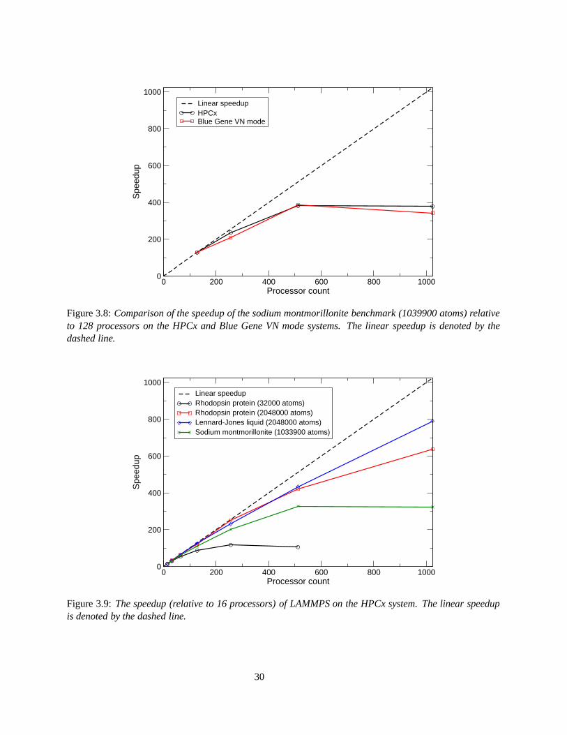
3.8 Comparison of the speedup of the sodium montmorillonite benchmark (1039900 atoms) rel-ative to 128 processors on the HPCx and Blue Gene VN mode systems. The linear speedupis denoted by the dashed line. . . . . . . . . . . . . . . . . . . . . . . . . . . . . . . . . . . 30
3.9 The speedup (relative to 16 processors) of LAMMPS on the HPCx system. The linearspeedup is denoted by the dashed line. . . . . . . . . . . . . . . . . . . . . . . . . . . . . . 30
v
3.10 Comparison of the time taken per timestep using the sodium montmorillonite benchmarkover 500 steps on the XCmaster system. . . . . . . . . . . . . . . . . . . . . . . . . . . . . 31
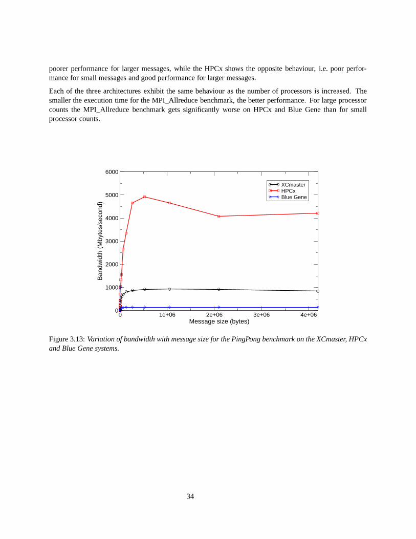
3.11 The performance of LAMMPS on the XCmaster system for each of the 3 benchmarks. . . . . 323.12 The performance of LAMMPS on the HPCx system for each of the 3 benchmarks. . . . . . . 323.13 Variation of bandwidth with message size for the PingPong benchmark on the XCmaster,
HPCx and Blue Gene systems. . . . . . . . . . . . . . . . . . . . . . . . . . . . . . . . . . 343.14 Variation of time with message size for the PingPong benchmark on the XCmaster, HPCx
and Blue Gene systems. . . . . . . . . . . . . . . . . . . . . . . . . . . . . . . . . . . . . . 353.15 Comparison of the time taken (at low processor counts) for the MPI_Allreduce benchmark
with two different message sizes of 32 B and 32 KB on the XCmaster, HPCx and Blue Genesystems. . . . . . . . . . . . . . . . . . . . . . . . . . . . . . . . . . . . . . . . . . . . . . 35
3.16 Comparison of the time taken (at high processor counts) for the MPI_Allreduce benchmarkwith two different message sizes of 32 B and 32 KB on the XCmaster, HPCx and Blue Genesystems. . . . . . . . . . . . . . . . . . . . . . . . . . . . . . . . . . . . . . . . . . . . . . 36
3.17 Comparison of the time taken (at low processor counts) for the MPI_Bcast benchmark withtwo different message sizes of 32 B and 32 KB on the XCmaster, HPCx and Blue Gene systems. 36
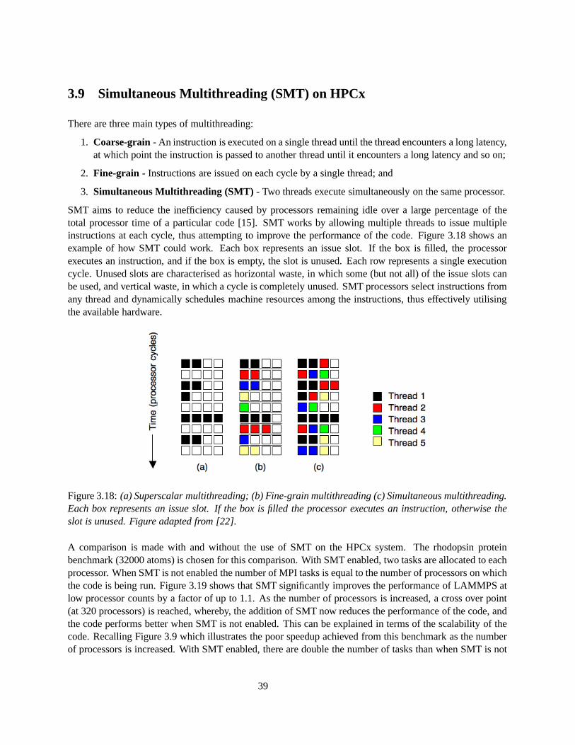
3.18 (a) Superscalar multithreading; (b) Fine-grain multithreading (c) Simultaneous multithread-ing. Each box represents an issue slot. If the box is filled the processor executes an instruc-tion, otherwise the slot is unused. Figure adapted from [22]. . . . . . . . . . . . . . . . . . 39
3.19 Comparison of the speedup of the rhodopsin protein benchmark (32000 atoms) with andwithout SMT enabled. A cross over point is reached at 320 processors. For less than 320processors SMT is found to improve performance, whereas for greater than 320 processorsSMT is found to degrade performance. . . . . . . . . . . . . . . . . . . . . . . . . . . . . . 41
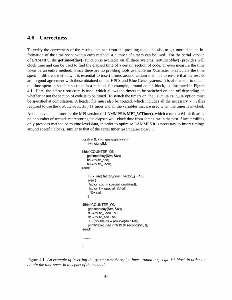
4.1 An example of inserting the gettimeofday() timer around a specific if block in orderto obtain the time spent in this part of the method. . . . . . . . . . . . . . . . . . . . . . . . 47
4.2 VAMPIR analysis of a single timestep for the rhodopsin protein benchmark (32000 atoms)run on 16 processors on the HPCx system. The timeline has been zoomed in the range 2.381- 2.383 seconds. . . . . . . . . . . . . . . . . . . . . . . . . . . . . . . . . . . . . . . . . . 51
4.3 VAMPIR analysis of a single timestep for rhodopsin protein benchmark (32000 atoms) runon 16 processors on the HPCx system. The timeline is an overview of the whole run. . . . . . 51
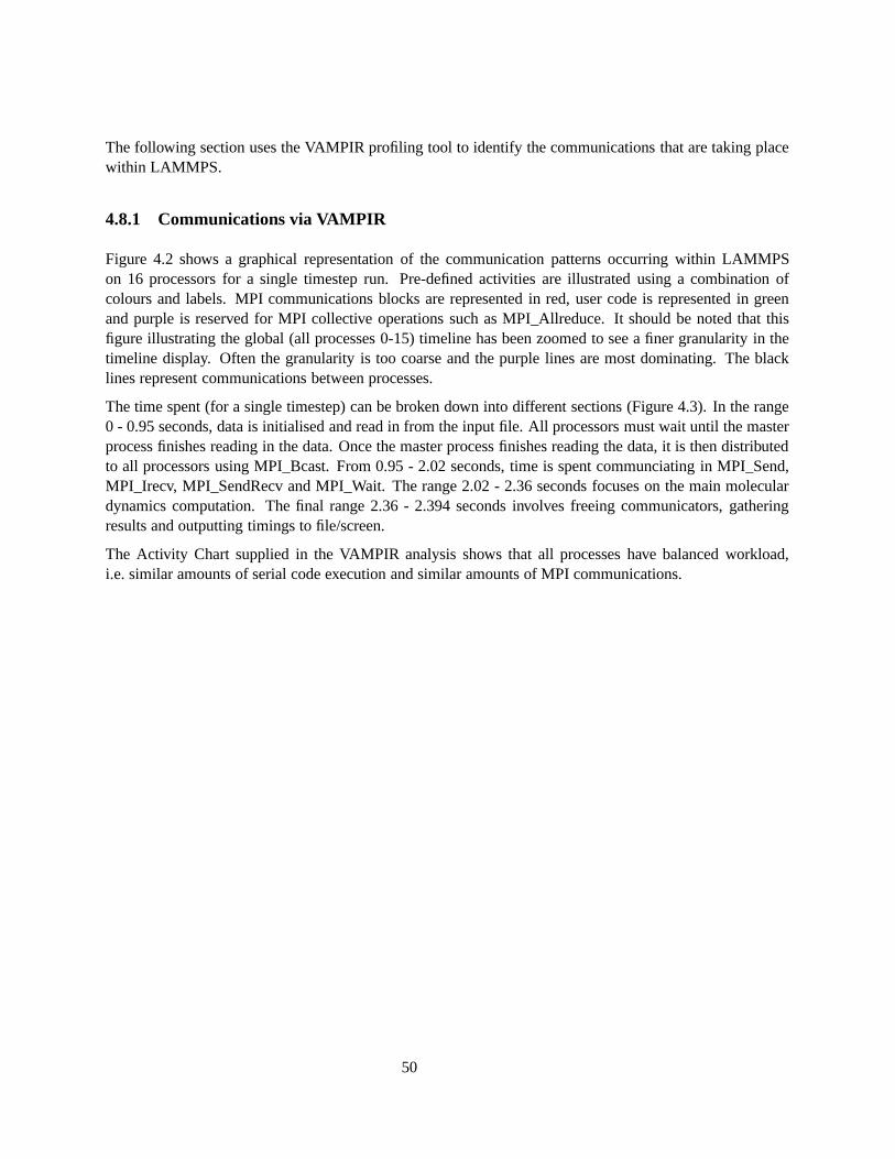
4.4 Comparison of the amount of time spent in different MPI routines (obtained using the MPI-Trace profiling tool) for the rhodopsin protein benchmark (2048000 atoms) for large pro-cessor counts on HPCx. . . . . . . . . . . . . . . . . . . . . . . . . . . . . . . . . . . . . . 53
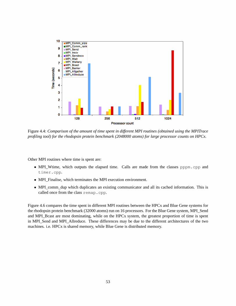
4.5 Comparison of the amount of time spent in different MPI routines (obtained using the TraceCollector and Analyzer tools) on XCmaster for the rhodopsin protein benchmark (32000atoms) run on 8 and 16 processors. . . . . . . . . . . . . . . . . . . . . . . . . . . . . . . . 54
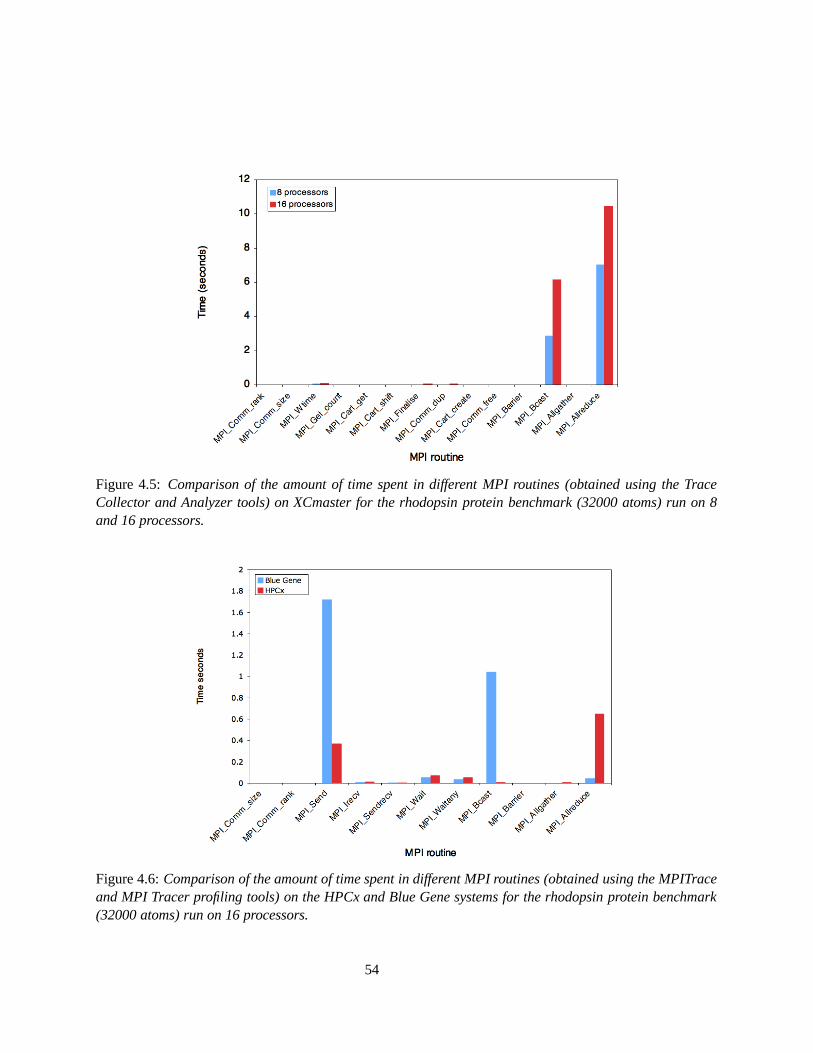
4.6 Comparison of the amount of time spent in different MPI routines (obtained using the MPI-Trace and MPI Tracer profiling tools) on the HPCx and Blue Gene systems for the rhodopsinprotein benchmark (32000 atoms) run on 16 processors. . . . . . . . . . . . . . . . . . . . 54
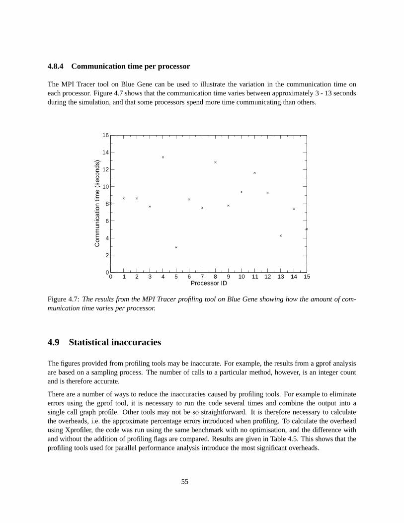
4.7 The results from the MPI Tracer profiling tool on Blue Gene showing how the amount ofcommunication time varies per processor. . . . . . . . . . . . . . . . . . . . . . . . . . . . 55
vi
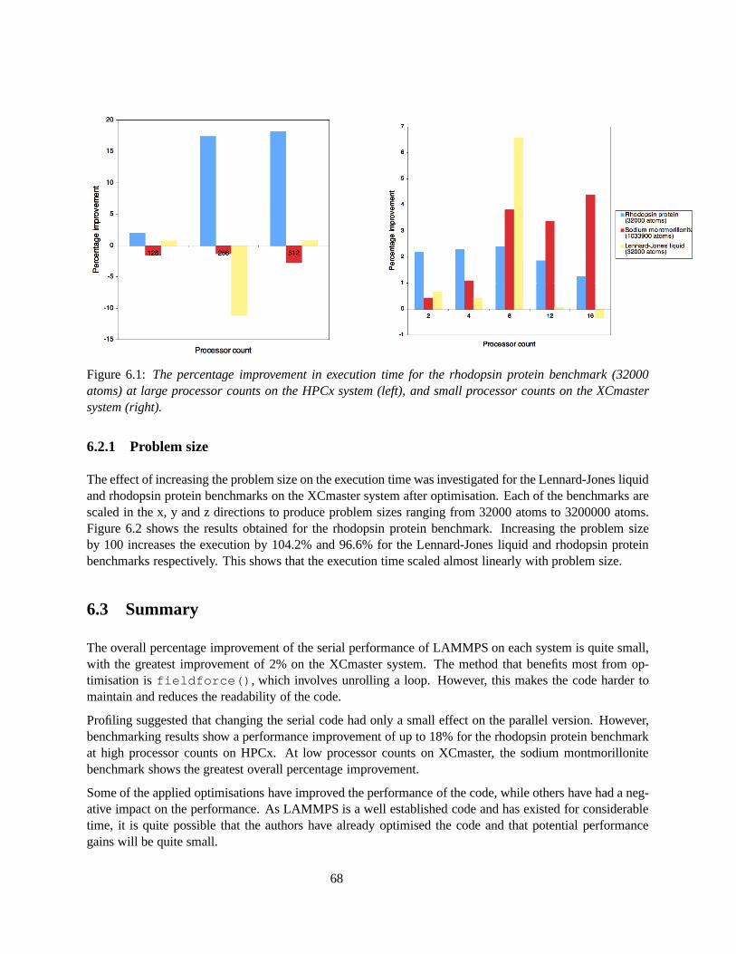
6.1 The percentage improvement in execution time for the rhodopsin protein benchmark (32000atoms) at large processor counts on the HPCx system (left), and small processor counts onthe XCmaster system (right). . . . . . . . . . . . . . . . . . . . . . . . . . . . . . . . . . . 68
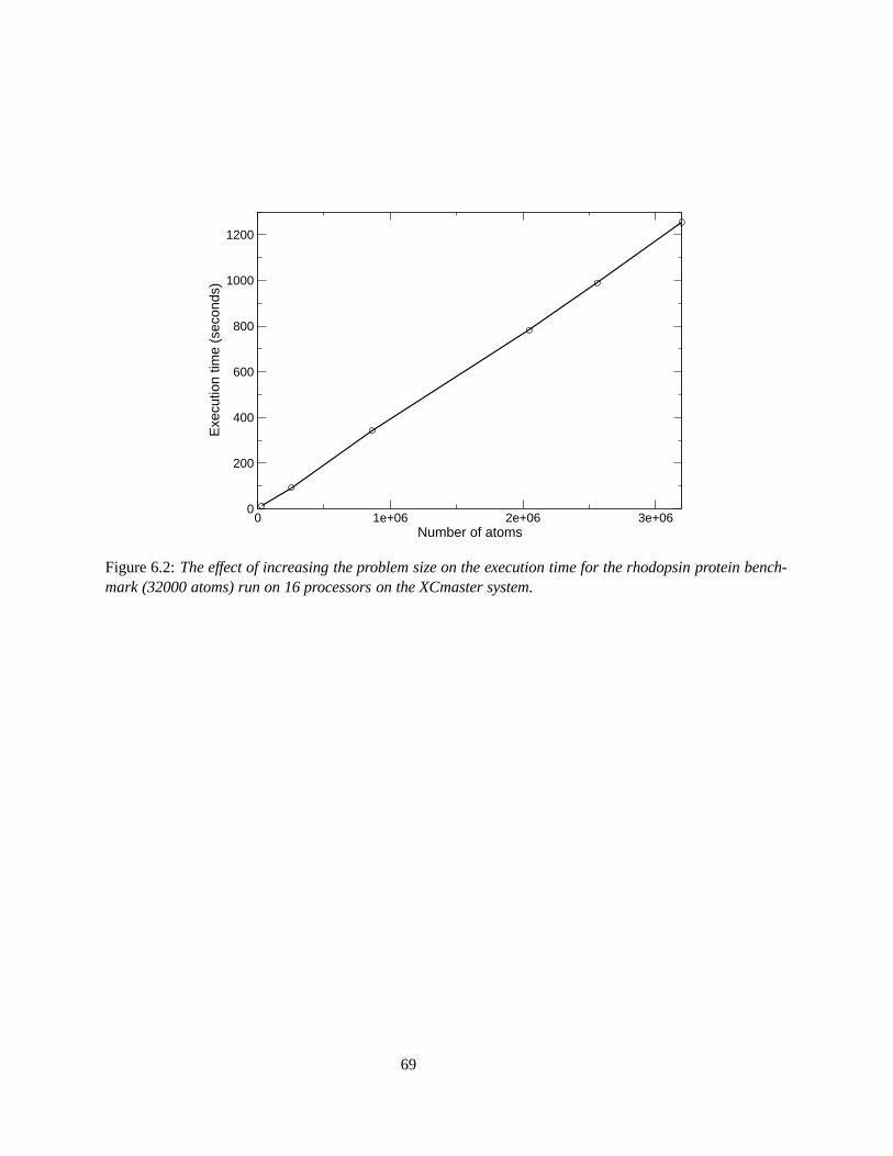
6.2 The effect of increasing the problem size on the execution time for the rhodopsin proteinbenchmark (32000 atoms) run on 16 processors on the XCmaster system. . . . . . . . . . . 69
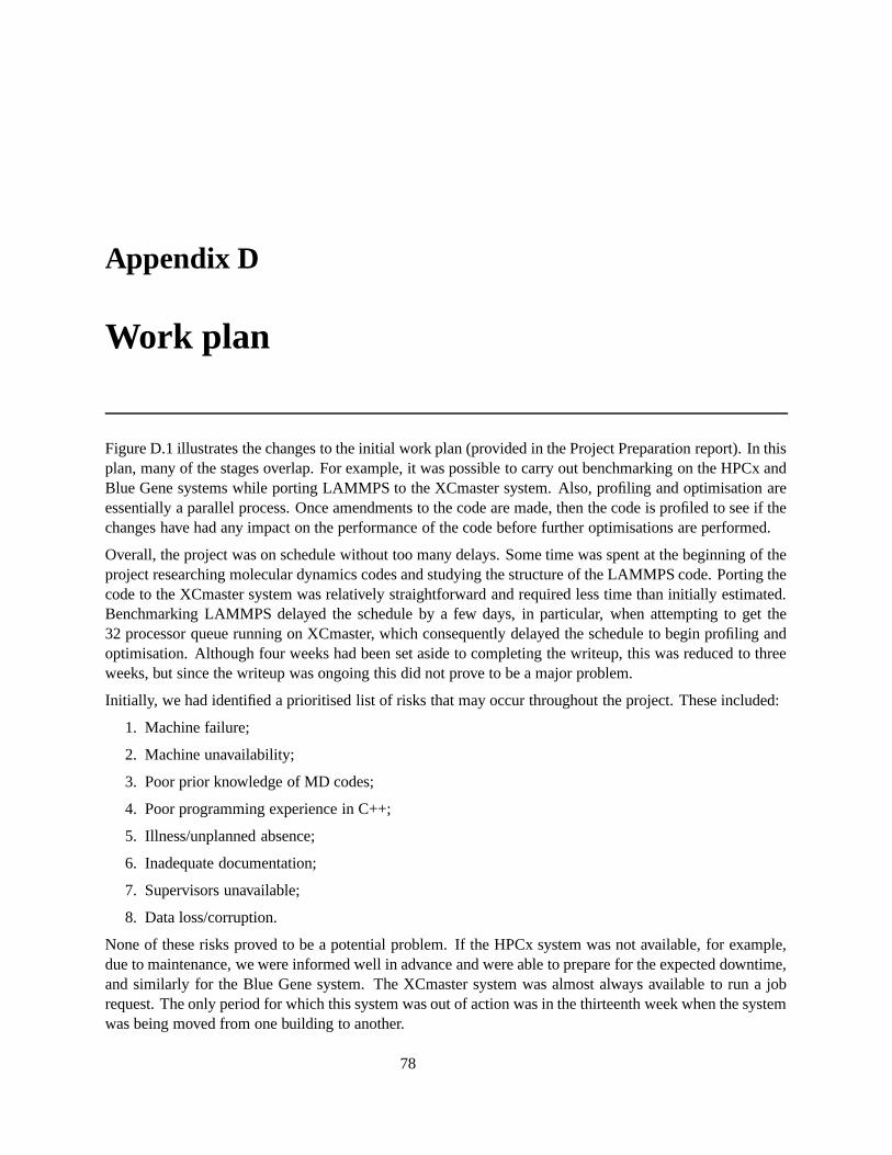
D.1 Diagrammatic work plan illustrating the changes to the initial work plan given in the ProjectPreparation report. The red arrows indicate the final work layout. . . . . . . . . . . . . . . 79
vii
Acknowledgements
First, I would like to express sincere thanks to Dr Fiona Reid, Michele Weiland and Dr Jim McCann fortheir expert supervision and guidance throughout the duration of this Masters dissertation, and indeed to allthe staff at EPCC who have contributed to this Masters degree. Special thanks must also go to Dr Hugo vander Hart (QUB) for his in-depth knowledge of the XCmaster system and Dr Chris Greenwell (Bangor) forsupplying the sodium montmorillonite benchmark.
For the various technical difficulties that I encountered, I would like to thank Ricky Rankin, Derek McPheeand Vaughan Purnell from Queen’s University Belfast for their continued support over the past 16 weeks. Iwould also like to thank my fellow students in EPCC for their friendship.
It remains for me to thank David for his confidence in me and for his interest, love and support.
I acknowledge financial support from UK Engineering and Physical Sciences Research Council (EPSRC).
Chapter 1
Introduction
High Performance Computing (HPC) involves using powerful computer systems to solve highly complexproblems and computationally intensive tasks. These include weather forecasting, drug development, com-puter aided engineering, molecular modelling and many more. These powerful systems are known assupercomputers and comprise of large numbers of processors linked together by an interconnect, whichenables the individual processors to communicate with each other to solve scientific problems. Suchproblems are defined by means of computer codes, which have been written to achieve the best possiblespeedup and to make efficient use of the available resources. One such code is the LAMMPS (Large ScaleAtomic/Molecular Massively Parallel Simulator) molecular dynamics simulation code, which is used in thisinvestigation.
The most powerful high performance computers are found in the Top 500 list [1], which contains the 500most powerful supercomputers in the world. The systems are ranked on the performance of the LINPACKbenchmark, which solves a dense system of linear equations. This particular benchmark is chosen becauseit is widely used and performance figures are available on most systems. Currently1 , the IBM Blue Gene/Lsystem installed at the US Department of Energy (DOE) Lawrence Livermore National Laboratory retainsthe number one position, while the Blue Gene and HPCx systems used in this study are at positions 148 and65 respectively (in the June 2007 list).
1.1 Aims and motivation
Molecular dynamics is a research area of intense topical interest enabling the simulation of very large andcomplex systems. Molecular dynamics codes are general purpose and are used in many disciplines, suchas condensed matter physics and biological modelling. Due to the large number of particles involved,molecular dynamics simulations typically require a very long time to run, and are thus computationallyexpensive. Any improvement in the runtime and scalability of molecular dynamics codes are beneficial tousers of these codes.
The aims are to learn the different techniques behind porting, profiling and optimising LAMMPS, as wellas to get familiar with the XCmaster system. This involves learning about the technicalities of the system
1at the time of writing
1
and the different profiling tools that are available. As this is a relatively new system installed at Queen’sUniversity in Belfast, little or no testing has been performed on the system. Therefore it would be of greatbenefit to the system administrators in Belfast, to have an idea of how the system is performing in comparisonto other systems, such as HPCx and Blue Gene.
The main objectives are:
1. To port LAMMPS to XCmaster at Queen’s University Belfast.
2. To benchmark and make comparisons between the performance of LAMMPS on XCmaster, HPCxand Blue Gene.
3. To carry out a performance analysis of LAMMPS on XCmaster, HPCx and Blue Gene.
4. To optimise LAMMPS on XCmaster, with the main aim to get LAMMPS to run faster, and then makecomparisons between the optimised versions on XCmaster, HPCx and Blue Gene.
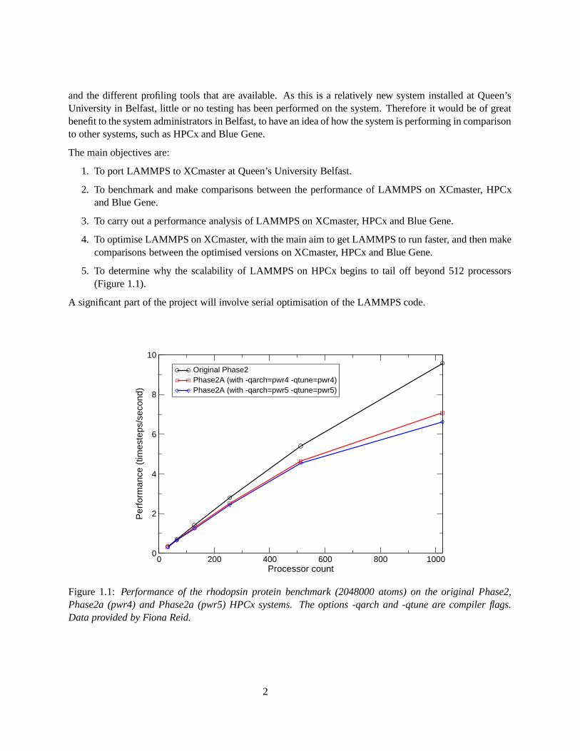
5. To determine why the scalability of LAMMPS on HPCx begins to tail off beyond 512 processors(Figure 1.1).
A significant part of the project will involve serial optimisation of the LAMMPS code.
0 200 400 600 800 1000Processor count
0
2
4
6
8
10
Per
form
ance
(tim
este
ps/s
econ
d)
Original Phase2Phase2A (with -qarch=pwr4 -qtune=pwr4)Phase2A (with -qarch=pwr5 -qtune=pwr5)
Figure 1.1: Performance of the rhodopsin protein benchmark (2048000 atoms) on the original Phase2,Phase2a (pwr4) and Phase2a (pwr5) HPCx systems. The options -qarch and -qtune are compiler flags.Data provided by Fiona Reid.
2
1.2 What is Molecular Dynamics?
Molecular dynamics is a technique used to compute the time evolution of a system of particles that interact.Molecular dynamics codes have become increasingly important in numerous areas of research, and in manyrespects are similar to real experiments. In particular, molecular dynamics techniques enable a wide range ofsimulation calculations to be performed on increasingly large and complex systems, ranging from condensedmatter physics to biological systems in areas such as disease and drug research. The codes are typicallygeneral purpose allowing many different types of physical system to be simulated. This flexibility meansthat the codes have many branches, however their flexible design may result in a variation of the exactphysics being modelled. Essentially this is because the codes have many branches which enable lots ofdifferent types of interactions to be modelled. The type (e.g metal, liquid, protein) and the forces whichapply to it are usually specified via the input file to the code. The codes are ususally flexible and generalpurpose, allowing them to be applied to many different types of systems and to perform a wide range offunctionalities. Such complex systems involve a large number of particles and cannot be easily solvedanalytically. They require powerful computer codes to simulate them. Often these codes are written inparallel, enabling them to utilise the very latest HPC facilities.
The most time-consuming part of a molecular dynamics simulation is the calculation of the forces acting oneach atom. Consider a classical system containing N particles. The movement of particles in this system isgoverned by the equations of motion of classical mechanics, i.e. Newton’s equations. The force on particlei due to all its neighbouring particles, scales as order N 2, where N is the total number of particles in thesimulation [2]. All particles interact with each other, but once the particles get too close they begin to repeleach other. By considering the interactions between atoms and molecules, the forces can then be thoughtof as being energies and so the potential energy due to the attraction and repulsion between atoms andmolecules is described using the Lennard-Jones potential [3], given by:
ΦLJ(r) = 4ε
[
(σ
r
)12−
(σ
r
)6]
, (1.1)
where σ is the depth of the well potential, ε is the bond energy and r is the position of the particle. Bothσ and ε are specific to the Lennard-Jones potential and have been chosen to fit the physical properties ofthe material. The term
(
1r
)12describes the short range repulsive potential due to the distortion of electron
clouds2 at small separations. When r is increased, the term(
1r
)6dominates. This describes the long range
attractive tail of the potential between two particles. The short range interactions are relatively easy to handlecomputationally as the particles are "close" to each other. For the long range potential an average over allparticles is taken.
In classical molecular dynamics, atoms are treated as point masses and simple Newtonian force rules areused to describe the interactions between the atoms. Newton’s second law is used to solve the Newtonianequations of motion:
Force = mass× acceleration, (1.2)
which are integrated in order to obtain an energy function that describes the energy of the structure of theatoms. Given the initial state of the atom, the energy function is then used to derive forces that determinethe position and velocity of the atoms at each time step. From the motion of the atoms, thermodynamic
2electron cloud - a region of negative charge surrounding an atomic nucleus.
3
statistics, such as relationships between different chemical states, are obtained. Many algorithms havebeen specifically designed to integrate Newton’s equations of motion. One such algorithm commonly usedfor time integration is the Verlet algorithm [4]. The Verlet algorithm is used to calculate trajectories3 ofmolecular dynamics simulations. First, the Taylor series of the position of the particle around time t, withtimestep ∆t is used. Let r(t) be the trajectory of a particle at time t. The Taylor expansion around time t isgiven by:
r(t + ∆t) = r(t) + v(t)∆t +f(t)
2m∆t2 +
∆t3
3!r + O(∆t4), (1.3)
where ∆t is the timestep used in the molecular dynamics simulation, r(t) is the present position, r(t + ∆t)is the new position of the particle, m is the mass of a particle, O(∆t4) is the local error in position of theVerlet integrator and F (t) is the resulting force on the particle.Similarly,
r(t−∆t) = r(t)− v(t)∆t +f(t)
2m∆t2 −
∆t3
3!r + O(∆t4). (1.4)
where r(t − ∆t) is the position of the previous timestep. By summing equations (1.3) and (1.4), andneglecting higher order terms (∆t4,∆r4) the following expression for the position of the particle is obtained:
r(t + ∆t) = 2r(t)− r(t−∆t) +f(t)
m∆t2. (1.5)
From equation (1.5) and knowledge of the trajectory, the velocity component, v(t), of the particle can bederived:
v(t) =r(t + ∆t)− r(t−∆t)
2∆t+ O(∆t2), (1.6)
where O(∆t4) is the local error in velocity.
The first derivative of r(t) with respect to t is equal to velocity. The second order derivative is equal toacceleration.
Interactions between particles are typically short range, allowing only neighbouring particles within a certaindistance, i.e. cut-off radius, to be considered. Any interactions beyond the cut-off radius are neglected.A long range correction to the potential can be introduced and included in the calculation of the shortrange potential, to compensate for the neglected calculations. Typically cut-off radii are used to reduce theamount of computation. The multi-purpose nature of molecular dynamics codes means that different typesof problems have to be solved and so selecting an appropriate cut-off radius is crucial to ensure an accurateand efficient computation. Usually the cut-off radius is determined by the physical problem that is beingsimulated.
1.3 What is LAMMPS?
LAMMPS stands for Large Scale Atomic/Molecular Massively Parallel Simulator. It’s a free open sourcemolecular dynamics code (under the GNU Public License) developed at Sandia National Laboratories, a USDepartment of Energy facility, and is used to solve classical physics equations, i.e. equations describing themotion of macroscopic objects [5].
3trajectory - a path a moving object follows through space.
4
LAMMPS can be used to simulate a wide range of materials such as large scale atomic and molecularsystems, using a combination of force fields and boundary conditions. It does this by integrating New-ton’s equations of motion for a system of interacting particles, given the initial boundary conditions. Theinteractions of the particles are via short or long range force fields. These force fields include pairwisepotentials, many body potentials, such as Embedded Atom Method (EAM), long range coulombics such asParticle-Particle Particle-Mesh (PPPM4) and also CHARMM5 force fields.
The code has been designed to run on large parallel systems, but can also run efficiently on a single pro-cessor machine. Its modular structure allows LAMMPS to be easily modified and extended to include newfunctionalities [5].
The code has been parallelised using MPI6 for parallel communications and uses spatial decomposition todivide the domain into small three-dimensional sub-domains. Each sub-domain is then assigned to eachprocessor on the parallel machine.
LAMMPS works by reading an input file, which specifies information about the atomic system, such asthe atom’s initial coordinates and number of timesteps used in the simulation. As the input file is read,information regarding the setup of the simulation is printed to a log file. LAMMPS then initialises theatomic system and periodically writes out the current state of the system after a user specified number oftimesteps have passed. The code can also checkpoint, such that if the system breaks down, data and resultshave not been lost, and the simulation can be restarted at the current position. The final state of the systemis then output to file. This includes a breakdown of total energies and the amount of time spent in thesimulation, as well as a breakdown of the percentage time spent in the main computations, such as pairwiseinteractions and bond times.
Development of LAMMPS started in the 1990’s and since then a number of versions have been released [5].The first version of LAMMPS was written in Fortran 77 and was released as LAMMPS 99. Subsequently thecode was converted to Fortran 90 and included features such as improved memory management (dynamicallocation in particular). The Fortran 90 version of the code was released in 2001. The code has since beenre-written in C++, and offers many new features including those from other molecular dynamics codes. Oneof the major improvements to the C++ code is that it now uses tables of neighbour lists to record nearbyparticles, thus reducing the amount of time LAMMPS spends computing pairwise interactions [6]. Theadvantage of C++ and its object-orientation is that modifications to the code can easily be made by simplydefining the new feature in two files, a header file .h and a .cpp file. The addition of a new class or methodshould not result in any side effects to the rest of the LAMMPS code. Subsequent releases simply containadditional features which add extra functionality to the code.
LAMMPS can be run on any number of processors. In principle, all the results should be identical, but theremay be some differences due to numerical round-off. The average energy or temperature should remain thesame.
There are five benchmarks supplied with the LAMMPS code. Details of each of these benchmarks are givenin Sections 3.1 and 3.2. Benchmarks are usually supplied to test a code, for example, to compare the resultsof a code with known results, and also to compare timings and performance across systems. The benchmarkssupplied with the LAMMPS code contain details of the simulations such as the number of timesteps over
4PPPM - am efficient method for calculating interactions in molecular simulations.5Chem at HARvard Molecular Mechanics - a force field used for molecular dynamics simulations.6Message Passing Interface - a library of routines used for communication between nodes running a parallel program.
5
which the simulation is run, and the simulation size, i.e. the number of atoms used in the simulation. Anotherbenchmark which will be considered is a user benchmark, namely sodium montmorillonite, supplied by DrChris Greenwell from the centre for computational science in the department of chemistry at the Universityof Wales, Bangor. This benchmark is based on benchmarks originally created by R.T Cygan at SandiaNational Laboratories.
1.4 Literature Review
Previous studies of the performance (measured in steps per second) of LAMMPS using a number of bench-marks (both user supplied and application supplied) have shown that LAMMPS generally scales well tolarge number of processors depending on the physical system being tested [6]. On the Blue Gene system(located at Lawrence Livermore National laboratories), LAMMPS has been run on up to 65536 processors.When run using the Lennard-Jones liquid benchmark (supplied with the code), LAMMPS was found tohave a scaled-size (4x4x4) parallel efficiency (referring to the ratio of ideal runtime to actual runtime) of89.5% on 65536 processors [7]. On HPCx it has been found to scale reasonably to 512 processors [8], witha scaled-size (4x4x4) parallel efficiency of 85% for the Lennard-Jones liquid benchmark [9].
A performance comparison of the benchmark results for a 124488 atom clay-polymer nanocomposite bench-mark (user supplied) and a 32000 atom rhodopsin benchmark (supplied with the code) for LAMMPS version2001 (Fortran 90) and 2004 (C++) respectively, show that in general the LAMMPS 2004 version appearsto scale better than the LAMMPS 2001 version. This difference in scaling may be explained in terms ofthe problem size and also the algorithms, which have been updated for the 2004 version of the code. Inparticular the addition of pre-computed neighbour lists in the LAMMPS 2004 version makes the serialruntime/performance timings between two and four times faster [10].
It has been found that the speedup of LAMMPS generally increases with the number of atoms used in thesimulation [6]. A performance comparsion of the LAMMPS 2005 version with the LAMMPS 2004 versionfor the application supplied rhodopsin benchmark shows that for more than 256 processors the speedup(relative to 32 processors) of LAMMPS 2004 is higher than that of LAMMPS 2005.
1.5 Outline of the dissertation
The structure of this thesis is based on the order in which the different stages of work have been carried out.Chapter 2 begins with a detailed discussion of each of the three architectures used for this analysis. A briefcomparison of previous results of LAMMPS on HPCx and Blue Gene is made. The final sections describethe act of porting LAMMPS to the XCmaster system. This includes details of installing the FFTW librariesand the LAMMPS code on the system, as well as any difficulties that were encountered. It also includesdetails for compiling the serial version of LAMMPS, and how the Makefiles (provided with the LAMMPScode) are amended in order to successfully compile LAMMPS on the HPCx and Blue Gene systems.
Chapter 3 describes in detail the different benchmarks that are provided with the LAMMPS codes and a usersupplied benchmark. The reasons for choosing these particular benchmarks are discussed. A comparison inthe performance of all three benchmarks are made on each system and results are presented and analysed.The breakdown of the run-time is also illustrated. As well as these benchmarks, Intel MPI Benchmarks
6
(IMB) are used to evaluate the performance of a PingPong, MPI_Allreduce and MPI_Bcast routine on eachsystem. The reproducibility of the results are discussed and a detailed outline of the attempts made to geta 32 processor queue working on the XCmaster system is provided. The chapter concludes by describ-ing simultaneous multithreading (SMT) on the HPCx system and discusses the results obtained for eachbenchmark.
Chapter 4 begins by discussing the reasons for carrying out a performance analysis, and provides a detaileddescription of the different profiling tools that are available on the systems, and what each tool is used for.The overheads associated with using these tools are discussed, and the correctness of the results have beenverified using a number of timers. The actual results obtained from using these profiling tools are given andare used to identify potential performance limitations in the LAMMPS code. Finally, the inaccuracies withusing profiling tools are discussed.
Chapter 5 describes the actual process of optimising the code. Each method (identified as limiting the codesperformance from Chapter 4) is individually examined and a number of possible optimisations are discussed,some of which may improve the performance of the code, others which may hinder the performance.
Chapter 6 discusses the performance of LAMMPS after optimisation. Results from profiling before andafter optimisation are presented. An analysis is given for both the serial and parallel versions of LAMMPS.
Finally, Chapter 7 discusses any conclusions that have been drawn and an evaluation of what has beenachieved, as well as possible suggestions for future work.
7
Chapter 2
Porting LAMMPS to XCmaster, HPCx andBlue Gene
2.1 Architectures
2.1.1 XCmaster
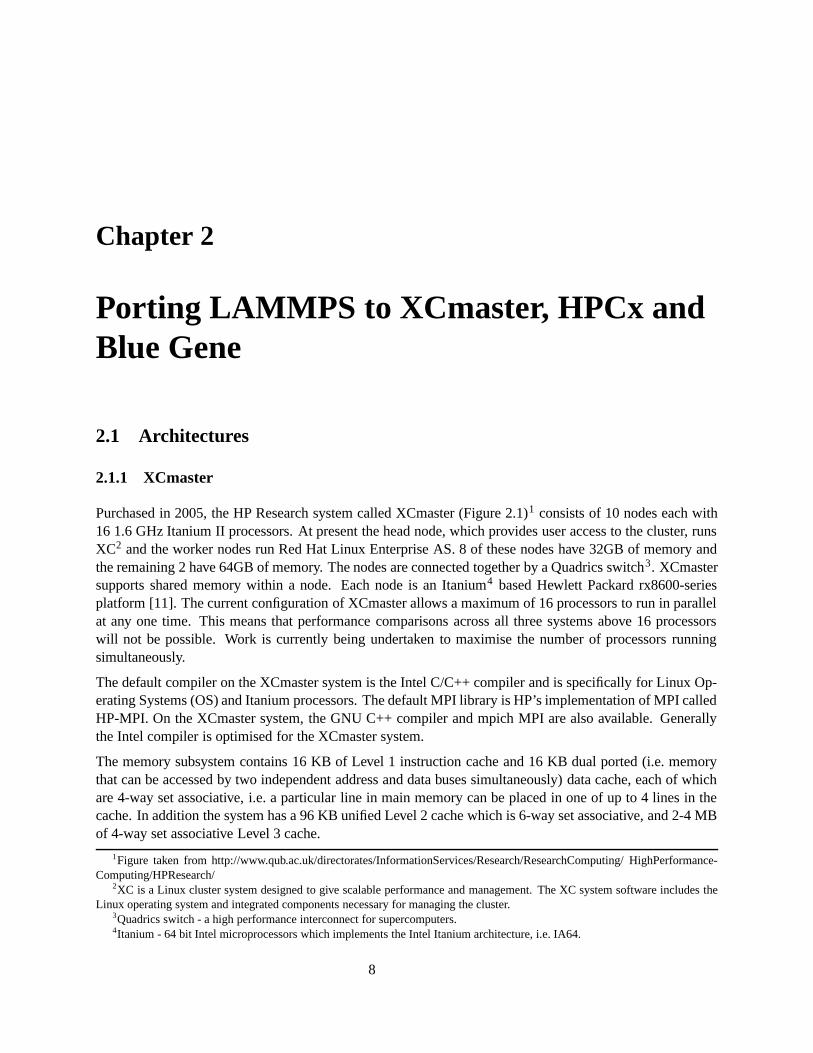
Purchased in 2005, the HP Research system called XCmaster (Figure 2.1)1 consists of 10 nodes each with16 1.6 GHz Itanium II processors. At present the head node, which provides user access to the cluster, runsXC2 and the worker nodes run Red Hat Linux Enterprise AS. 8 of these nodes have 32GB of memory andthe remaining 2 have 64GB of memory. The nodes are connected together by a Quadrics switch3. XCmastersupports shared memory within a node. Each node is an Itanium4 based Hewlett Packard rx8600-seriesplatform [11]. The current configuration of XCmaster allows a maximum of 16 processors to run in parallelat any one time. This means that performance comparisons across all three systems above 16 processorswill not be possible. Work is currently being undertaken to maximise the number of processors runningsimultaneously.
The default compiler on the XCmaster system is the Intel C/C++ compiler and is specifically for Linux Op-erating Systems (OS) and Itanium processors. The default MPI library is HP’s implementation of MPI calledHP-MPI. On the XCmaster system, the GNU C++ compiler and mpich MPI are also available. Generallythe Intel compiler is optimised for the XCmaster system.
The memory subsystem contains 16 KB of Level 1 instruction cache and 16 KB dual ported (i.e. memorythat can be accessed by two independent address and data buses simultaneously) data cache, each of whichare 4-way set associative, i.e. a particular line in main memory can be placed in one of up to 4 lines in thecache. In addition the system has a 96 KB unified Level 2 cache which is 6-way set associative, and 2-4 MBof 4-way set associative Level 3 cache.
1Figure taken from http://www.qub.ac.uk/directorates/InformationServices/Research/ResearchComputing/ HighPerformance-Computing/HPResearch/
2XC is a Linux cluster system designed to give scalable performance and management. The XC system software includes theLinux operating system and integrated components necessary for managing the cluster.
3Quadrics switch - a high performance interconnect for supercomputers.4Itanium - 64 bit Intel microprocessors which implements the Intel Itanium architecture, i.e. IA64.
8
The batch system software is called Load Sharing Facility (LSF). All production runs should be submittedvia a batch submission script to the backend (using the bsub command), since other users may be workingon the same master node, which may affect the timings obtained for the benchmarks if run interactively.
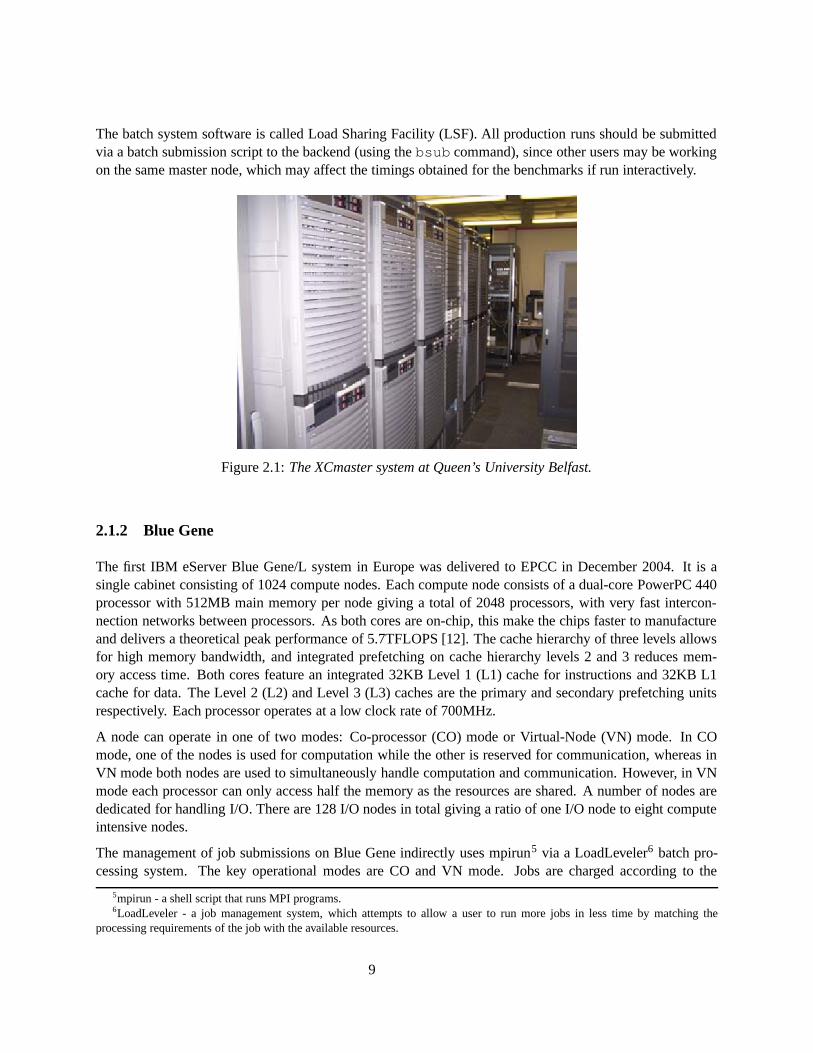
Figure 2.1: The XCmaster system at Queen’s University Belfast.
2.1.2 Blue Gene
The first IBM eServer Blue Gene/L system in Europe was delivered to EPCC in December 2004. It is asingle cabinet consisting of 1024 compute nodes. Each compute node consists of a dual-core PowerPC 440processor with 512MB main memory per node giving a total of 2048 processors, with very fast intercon-nection networks between processors. As both cores are on-chip, this make the chips faster to manufactureand delivers a theoretical peak performance of 5.7TFLOPS [12]. The cache hierarchy of three levels allowsfor high memory bandwidth, and integrated prefetching on cache hierarchy levels 2 and 3 reduces mem-ory access time. Both cores feature an integrated 32KB Level 1 (L1) cache for instructions and 32KB L1cache for data. The Level 2 (L2) and Level 3 (L3) caches are the primary and secondary prefetching unitsrespectively. Each processor operates at a low clock rate of 700MHz.
A node can operate in one of two modes: Co-processor (CO) mode or Virtual-Node (VN) mode. In COmode, one of the nodes is used for computation while the other is reserved for communication, whereas inVN mode both nodes are used to simultaneously handle computation and communication. However, in VNmode each processor can only access half the memory as the resources are shared. A number of nodes arededicated for handling I/O. There are 128 I/O nodes in total giving a ratio of one I/O node to eight computeintensive nodes.
The management of job submissions on Blue Gene indirectly uses mpirun5 via a LoadLeveler6 batch pro-cessing system. The key operational modes are CO and VN mode. Jobs are charged according to the
5mpirun - a shell script that runs MPI programs.6LoadLeveler - a job management system, which attempts to allow a user to run more jobs in less time by matching the
processing requirements of the job with the available resources.
9
partitions of LoadLeveler. Currently, there are only four sizes of partition: 32, 128, 512 and 1024 proces-sors. Therefore whenever a 64 processor job is submitted and run on Blue Gene, LoadLeveler reserves a 128node partition. 64 nodes/processors are used for the users job with the other 64 nodes/processors left idle.This is the physical limit of the architecture of the machine and depends on the design of the torus networkused to wire individual components together. No other configurations are possible [12].
Nodes are interconnected via five networks, each with different functionalities [12]:
• a three-dimensional torus network for point-to-point communications between nodes;
• a global broadcast tree for collective operations and allowing compute nodes to communicate withtheir I/O nodes, which then communicate to other systems;
• a global barrier and interrupt tree network for fast barrier synchronisation; and
• two GigaByte (GB) ethernets for connections to other systems.
The design of the Blue Gene system (Figure 2.2)7 uses slanted walls to separate the hot air at the top of thesystem from the cold air at the bottom, which allows for better cooling.
Figure 2.2: The IBM Blue Gene/L system at EPCC in Edinburgh.
2.1.3 HPCx
In November 2006, the HPCx Phase 3 system began user service [6] (Figure 2.3)8. It is currently the UKnational high performance computing service (run by UoE HPCx Ltd), and is located at CCLRC Daresbury
7Figure taken from http://www.epcc.ed.ac.uk/facilities/blue-gene/8Figure taken from http://www.hpcx.ac.uk/about/gallery/
10
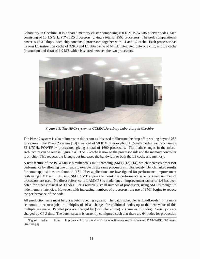
Laboratory in Cheshire. It is a shared memory cluster comprising 160 IBM POWER5 eServer nodes, eachconsisting of 16 1.5 GHz POWER5 processors, giving a total of 2560 processors. The peak computationalpower is 15.3 Tflops. Each chip contains 2 processors together with L1 and L2 cache. Each processor hasits own L1 instruction cache of 32KB and L1 data cache of 64 KB integrated onto one chip, and L2 cache(instruction and data) of 1.9 MB which is shared between the two processors.
Figure 2.3: The HPCx system at CCLRC Daresbury Laboratory in Cheshire.
The Phase 2 system is also of interest in this report as it is used to illustrate the drop off in scaling beyond 256processors. The Phase 2 system [13] consisted of 50 IBM pSeries p690 + Regatta nodes, each containing32 1.7GHz POWER4+ processors, giving a total of 1600 processors. The main changes in the micro-architecture can be seen in Figure 2.49. The L3 cache is now on the processor side and the memory controlleris on-chip. This reduces the latency, but increases the bandwidth to both the L3 cache and memory.
A new feature of the POWER5 is simultaneous multithreading (SMT) [13] [14], which increases processorperformance by allowing two threads to execute on the same processor simultaneously. Benchmarked resultsfor some applications are found in [15]. User applications are investigated for performance improvementboth using SMT and not using SMT. SMT appears to boost the performance when a small number ofprocessors are used. No direct reference to LAMMPS is made, but an improvement factor of 1.4 has beennoted for other classical MD codes. For a relatively small number of processors, using SMT is thought tohide memory latencies. However, with increasing numbers of processors, the use of SMT begins to reducethe performance of the code.
All production runs must be via a batch queuing system. The batch scheduler is LoadLeveler. It is moreeconomic to request jobs in multiples of 16 as charges for additional nodes up to the next value of thismultiple are made. Parallel jobs are charged by (wall clock time) × (number of nodes). Serial jobs arecharged by CPU time. The batch system is currently configured such that there are 64 nodes for production
9Figure taken from http://www-941.ibm.com/collaboration/wiki/download/attachments/1927/POWER4-5-System-Structure.png
11
Figure 2.4: Comparison of the Power4 and Power5 HPCx architectures.
runs, 26 nodes for capacity10 runs, 2 nodes for interactive runs and finally 12 nodes available to specificprojects. Other nodes are available for logging in and I/O.
2.2 Comparisons of LAMMPS results on different architectures
A comparison of communication benchmarking on HPCx Phase2 and Phase2a shows a small difference inthe performance on these two systems [16]. Phase2a is essentially Phase3, i.e. both phases have the samearchitecture, except Phase3 has a greater number of processors. The maximum number of tasks that can besubmitted on both phases remains the same, i.e. 1024. The scaling of LAMMPS is generally good up to256 processors but drops off beyond 256. Comparing the performance of a 2048000 atom rhodopsin systemusing LAMMPS 2001, it is found that Phase2 shows better performance than Phase2a, and also the scalingon Phase2a is poorer, resulting in a high performance difference at 1024 processors between both phases.It is thought that this may be due to a sensitivity to memory latency. Little difference is observed betweenthe platforms for the Bcast and Allreduce benchmarks. Improved memory bandwidth on Phase2a isbelieved to be the reason for better performance. For small processor counts, the difference in performanceis given by a factor of the clock frequency ratio. As the number of processors is increased, the scaling onPhase2a begins to drop off leading to a higher difference in performance on 1024 processors.
For large processor counts on HPCx, there is a variability in the results obtained. This is most likely due toOS interruptions such as system noise caused by periodic OS clock ticks, or hardware interrupts. I/O beingshared between all users may also be a factor. This was observed for 512 and 1024 processor runs. However,to compensate for these inaccuracies, the code was run a number of times with the lowest execution timesbeing noted.
10Capacity runs - jobs that use small numbers of processors for large amounts of time [14].
12
A performance comparison of LAMMPS run on the HPCx and Blue Gene systems again shows that LAMM-PS generally scales well [17] [18]. It was found that the performance per processor on Blue Gene is worsethan that of HPCx, however the scaling is better for large numbers of processors. This is as expected sincethe Blue Gene system consists of a large number of less powerful processors. VN mode was also found togive better performance than CO mode on all processor counts. Comparing the performance of a 1012736atom clay polymer system using LAMMPS 2001, the simulation was found to be approximately 4.2 timesfaster on HPCx at 128 processors, but as the number of processors increased the Blue Gene system showedbetter scaling. This may be due to better memory bandwidth on the processors. Even though HPCx hashigher clock frequencies and better floating point units, these advantages were less than expected. In termsof cost factors such as power consumption, efficient use of space and hardware cost, the Blue Gene systemis more cost effective than the HPCx system [17].
2.3 Porting to XCmaster
The process of porting LAMMPS to the XCmaster system requires two main stages. First, the FFTW 2.1.5library must be installed, as this is a necessary requirement by LAMMPS. The next stage involves portingthe LAMMPS 2006 version to the XCmaster system, which simply means installing the LAMMPS code onthe system and ensuring that it compiles and runs, and produces the correct results.
2.3.1 FFTW code
FFTW (Fastest Fourier Transforms in the West) is a collection of ANSI C library routines which are usedto compute the Discrete Fourier Transform (DFT) in one or more dimensions [19]. A Fourier Transform issimply a mathematical tool that defines a relationship between a signal in the time domain and representsit in the frequency domain. In other words, its a linear operation that maps functions to other functions,enabling the mathematical problem to be easily solved. The FFTW library is very portable and should workon any system. The FFTW library can be downloaded from the FFTW website11 and is freely availableunder the GNU Public License. The FFTW library uses novel code generation as well as self-optimisingtechniques to reduce the amount of calculation required, thus achieving faster calculation of DFTs andimproved performance than other publicly available FFT implementations [19]. FFTW uses the divide-and-conquer method, which divides a problem into several sub-problems. Each of the sub-problems are thensolved recursively, and the solutions are combined to create a solution for the original problem. This allowsFFTW to take advantage of the memory hierarchy.
FFTW works by adapting the DFT algorithm to the architecture on which it is installed, in order to achievebest performance. The computation of the transform can be split into two phases. In the first phase, theFFTW’s "planner" is called. The planner is used to produce a plan, which details the information on thefastest way to compute the transform on your machine. This information is then passed to the "executor",which computes the actual transform. The complexity of the algorithms used are O(NlogN). This plan canbe used many times and is then destroyed when no longer required.
There are two versions of FFTW available, FFTW 2.1.5 and FFTW 3.0.1. The choice of which version touse essentially depends on the code being implemented. FFTW 3.0.1 does not include parallel transforms
11www.fftw.org - developed at Massachusetts Institute of Technology (MIT) by Matteo Frigo and Steven G. Johnson.
13
for distributed memory systems, whereas FFTW 2.1.5 includes parallel transforms for both shared anddistributed memory systems. On a shared memory system, the FFTW is implemented using Posix threads (astandard that defines an Application Program Interface (API) for creating and manipulating threads), whileon the distributed memory system, the FFTW implementation is based on MPI. Also, in FFTW 3.0.1 theAPI has been changed and is no longer compatible with LAMMPS and thus version 2.1.5 must be used.
2.3.2 Installing FFTW on XCmaster
In order to use the PPPM option in LAMMPS for long range Coulombics, a one-dimensional FFTW librarymust be installed on the platform. From the documentation provided on the XCmaster system, it is unclearwhich version of FFTW is actually installed. For safe practice, and knowing that LAMMPS specificallyrequires version 2.1.5, it was necessary to download and install this particular version on the system. Anadvantage of installing FFTW on the system is that debugging can be done (if necessary) and the levelof optimisation used during compilation is known. First, both single and double precision versions of thelibraries are installed. Even though LAMMPS usually requires the double precision version for increasedaccuracy, it is often useful to have both versions installed on the system.
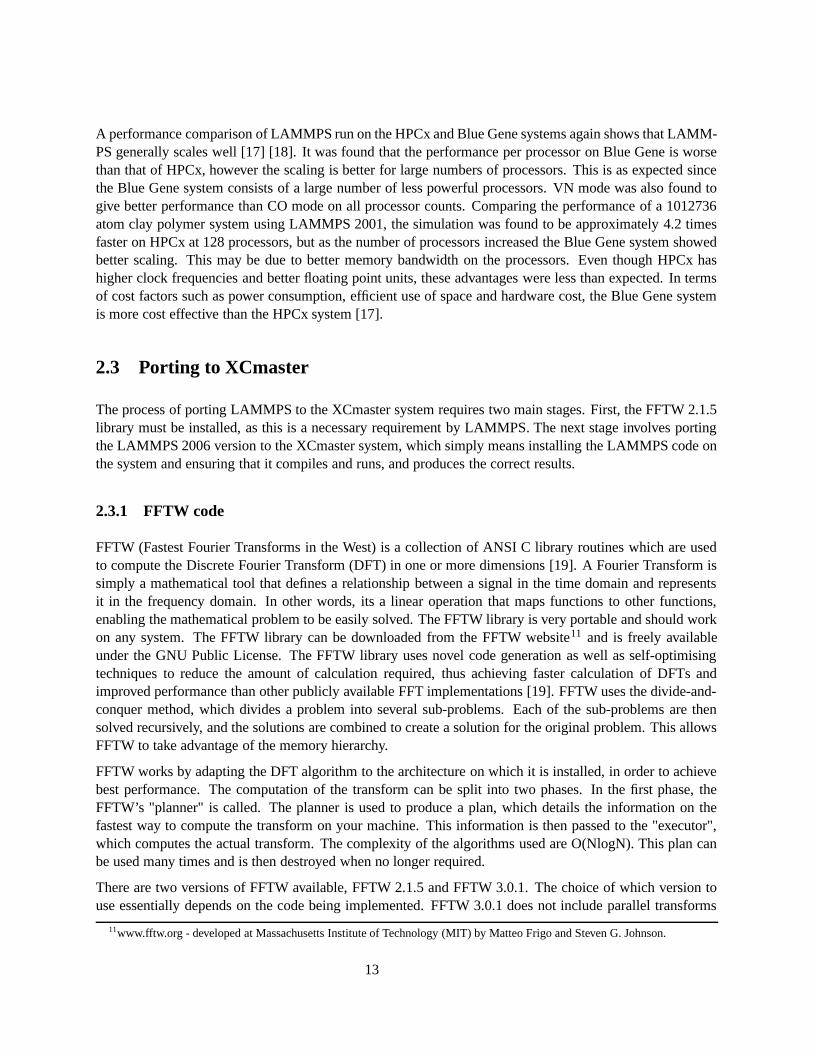
Figure 2.5 shows an example of a bash shell script that was used to build both the single and double precisionlibraries on the XCmaster system. The option -enable-type-prefix is used to install the FFTWlibraries and header files prefixed with the character "d" or "s", depending on whether the compilation issingle or double precision. To ensure that the FFTW library was correctly installed, tests are provided in thetest directory.The standard version of LAMMPS on XCmaster can be built by specifying the full path (in which the FFTWlibrary is installed) in the Makefile, together with the link option -ldfftw, which is used to link the doubleprecision version. The -O3 optimisation flag is added to the Makefile which is used to compile the code.
2.3.3 Installing LAMMPS on XCmaster
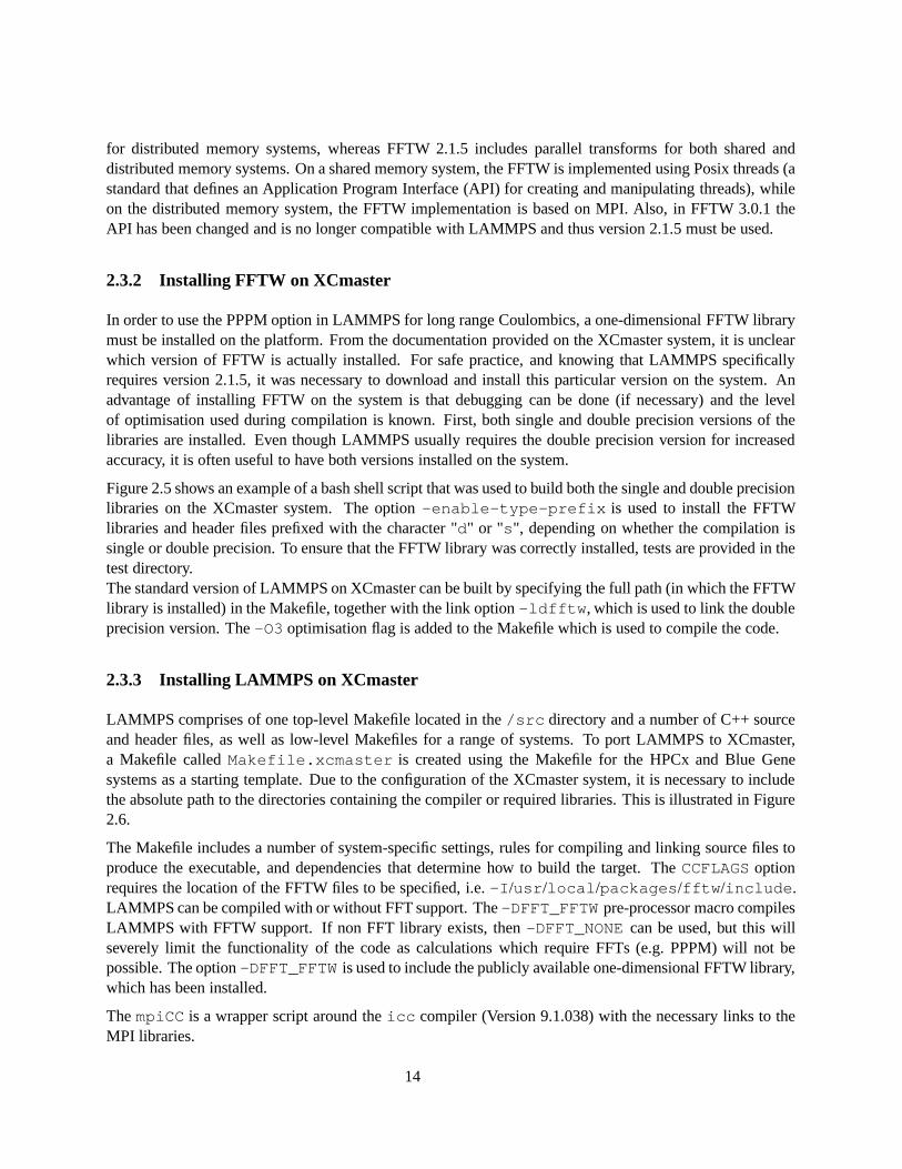
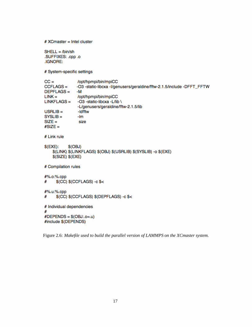
LAMMPS comprises of one top-level Makefile located in the /src directory and a number of C++ sourceand header files, as well as low-level Makefiles for a range of systems. To port LAMMPS to XCmaster,a Makefile called Makefile.xcmaster is created using the Makefile for the HPCx and Blue Genesystems as a starting template. Due to the configuration of the XCmaster system, it is necessary to includethe absolute path to the directories containing the compiler or required libraries. This is illustrated in Figure2.6.
The Makefile includes a number of system-specific settings, rules for compiling and linking source files toproduce the executable, and dependencies that determine how to build the target. The CCFLAGS optionrequires the location of the FFTW files to be specified, i.e. -I/usr/local/packages/fftw/include.LAMMPS can be compiled with or without FFT support. The -DFFT_FFTW pre-processor macro compilesLAMMPS with FFTW support. If non FFT library exists, then -DFFT_NONE can be used, but this willseverely limit the functionality of the code as calculations which require FFTs (e.g. PPPM) will not bepossible. The option -DFFT_FFTW is used to include the publicly available one-dimensional FFTW library,which has been installed.
The mpiCC is a wrapper script around the icc compiler (Version 9.1.038) with the necessary links to theMPI libraries.
14
Figure 2.5: A bash shell script to build the single and double precision FFTW 2.1.5 on the XCmaster system.
A few modifications to the source code are required. First, the name of the header files in the source directoryof LAMMPS must be modified so that they compile correctly against FFTW 2.1.5. The file fft3d.h needsto be altered so that correct FFTW header files are picked up. The "d" means using the double precisionFFTW header files.
Since the XCmaster system is a relatively new machine, there are very few users on the system. Most of thecurrent users are Fortran based programmers and so one of the problems encountered involved the licensefor the C++ compiler having expired. An error message was displayed, and it was necessary to contactsystem administration in order to get the licence renewed. It also took a considerable amount of time tolocate the latest version of this compiler, as a number of versions of the compiler had been installed indifferent directories.
Using optimisation switches when compiling code can significantly improve the execution time of the code.The following optimisation flags were tested and a brief description of each is given below:[-O0] [-O2] [-O3] -fast .
• The -O0 option is the default optimisation. It attempts to reduce the execution time and provides fulldebugging support.
• The -O2 option is a form of low level optimisation, and eliminates redundant or unused code. This isthe default option on the XCmaster system.
15
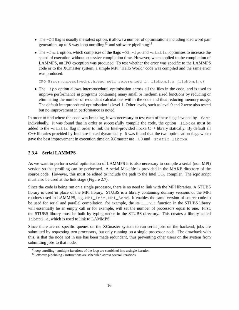
• The -O3 flag is usually the safest option, it allows a number of optimisations including load word pairgeneration, up to 8-way loop unrolling12 and software pipelining13 .
• The -fast option, which comprises of the flags -O3, -ipo and -static, optimises to increase thespeed of execution without excessive compilation time. However, when applied to the compilation ofLAMMPS, an IPO exception was produced. To test whether the error was specific to the LAMMPScode or to the XCmaster system, a simple MPI "Hello World" code was compiled and the same errorwas produced:
IPO Error:unresolved:pthread_self referenced in libhpmpi.a (libhpmpi.o)
• The -ipo option allows interprocedural optimisation across all the files in the code, and is used toimprove performance in programs containing many small or medium sized functions by reducing oreliminating the number of redundant calculations within the code and thus reducing memory usage.The default interprocedural optimisation is level 1. Other levels, such as level 0 and 2 were also testedbut no improvement in performance is noted.
In order to find where the code was breaking, it was necessary to test each of these flags invoked by -fastindividually. It was found that in order to successfully compile the code, the option -libcxa must beadded to the -static flag in order to link the Intel-provided libcxa C++ library statically. By default allC++ libraries provided by Intel are linked dynamically. It was found that the two optimisation flags whichgave the best improvement in execution time on XCmaster are -O3 and -static-libcxa.
2.3.4 Serial LAMMPS
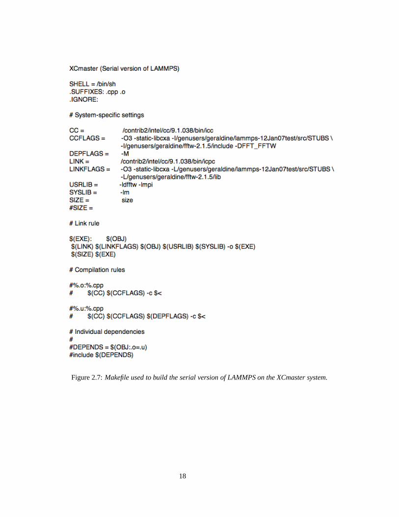
As we want to perform serial optimisation of LAMMPS it is also necessary to compile a serial (non MPI)version so that profiling can be performed. A serial Makefile is provided in the MAKE directory of thesource code. However, this must be edited to include the path to the Intel icc compiler. The icpc scriptmust also be used at the link stage (Figure 2.7).
Since the code is being run on a single processor, there is no need to link with the MPI libraries. A STUBSlibrary is used in place of the MPI library. STUBS is a library containing dummy versions of the MPIroutines used in LAMMPS, e.g. MPI_Init, MPI_Send. It enables the same version of source code tobe used for serial and parallel compilation, for example, the MPI_Init function in the STUBS librarywill essentially be an empty call or for example, will set the number of processors equal to one. First,the STUBS library must be built by typing make in the STUBS directory. This creates a library calledlibmpi.a, which is used to link to LAMMPS.
Since there are no specific queues on the XCmaster system to run serial jobs on the backend, jobs aresubmitted by requesting two processors, but only running on a single processor node. The drawback withthis, is that the node not in use has been made redundant, thus preventing other users on the system fromsubmitting jobs to that node.
12loop unrolling - multiple iterations of the loop are combined into a single iteration.13Software pipelining - instructions are scheduled across several iterations.
16
Figure 2.6: Makefile used to build the parallel version of LAMMPS on the XCmaster system.
17
Figure 2.7: Makefile used to build the serial version of LAMMPS on the XCmaster system.
18
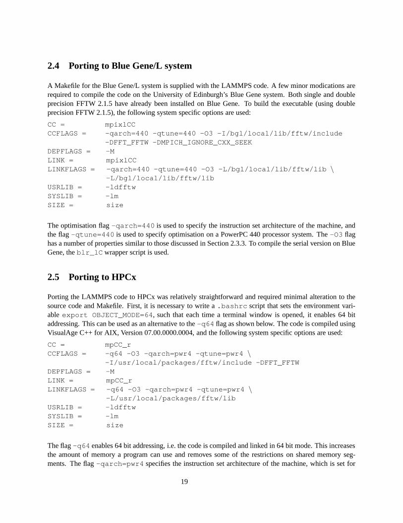
2.4 Porting to Blue Gene/L system
A Makefile for the Blue Gene/L system is supplied with the LAMMPS code. A few minor modications arerequired to compile the code on the University of Edinburgh’s Blue Gene system. Both single and doubleprecision FFTW 2.1.5 have already been installed on Blue Gene. To build the executable (using doubleprecision FFTW 2.1.5), the following system specific options are used:
CC = mpixlCCCCFLAGS = -qarch=440 -qtune=440 -O3 -I/bgl/local/lib/fftw/include
The optimisation flag -qarch=440 is used to specify the instruction set architecture of the machine, andthe flag -qtune=440 is used to specify optimisation on a PowerPC 440 processor system. The -O3 flaghas a number of properties similar to those discussed in Section 2.3.3. To compile the serial version on BlueGene, the blr_lC wrapper script is used.
2.5 Porting to HPCx
Porting the LAMMPS code to HPCx was relatively straightforward and required minimal alteration to thesource code and Makefile. First, it is necessary to write a .bashrc script that sets the environment vari-able export OBJECT_MODE=64, such that each time a terminal window is opened, it enables 64 bitaddressing. This can be used as an alternative to the -q64 flag as shown below. The code is compiled usingVisualAge C++ for AIX, Version 07.00.0000.0004, and the following system specific options are used:
CC = mpCC_rCCFLAGS = -q64 -O3 -qarch=pwr4 -qtune=pwr4 \
The flag -q64 enables 64 bit addressing, i.e. the code is compiled and linked in 64 bit mode. This increasesthe amount of memory a program can use and removes some of the restrictions on shared memory seg-ments. The flag -qarch=pwr4 specifies the instruction set architecture of the machine, which is set for
19
the POWER4 HPCx system. Finally the flag -qtune=pwr4 biases optimisation towards execution on thePOWER4 HPCx system.
To compile the serial version on HPCx, the xlC_r compiler is used. The _r stands for re-entrant, denotingthat the compiler generates thread safe code. It allows access to numerical libraries which are stable andallow 32 and 64 bit addressing.
2.6 Summary
Porting this application to XCmaster for the first time resulted in several problems, most of which were dueto the configuration of the XCmaster system. A significant amount of time was spent in addressing theseissues, but a successful port was achieved. Both serial and parallel versions of the code are running on allthree systems. The FFTW 2.1.5 library has also been successfully installed on the XCmaster system.
The next chapter presents and analyses the performance of LAMMPS on each system.
20
Chapter 3
Benchmarking
This chapter presents results from three different benchmarks, two of which are supplied with the LAMMPScode and a realistic scientific user benchmark supplied by Dr Chris Greenwell (Bangor).
The two benchmarks supplied with the code have been chosen because they are stable and scale well tolarge numbers of processors. They include the rhodopsin protein benchmark which uses the Particle-ParticleParticle-Mesh (PPPM) method (an efficient method for calculating interactions in molecular simulations),and a Lennard-Jones liquid benchmark for comparison. The benchmarks have been previously run on theHPCx and Blue Gene systems and so results are available to make comparisons with the results that areobtained in this project. The user supplied benchmark, namely sodium montmorillonite, was chosen sinceit can be applied to real user applications. The main difference between these three benchmarks is thatthe user benchmark includes disk I/O, which has been found to affect the scalability of the code on largenumbers of processors. The primary goal is to investigate the performance of the LAMMPS simulation codeon XCmaster, HPCx and Blue Gene. Benchmarking is carried out on each of the three architectures and aperformance comparison is made.
3.1 Benchmarks supplied with LAMMPS code
Each of these benchmarks has 32000 atoms and typically runs for 100 timesteps, although this can be alteredin the input script. The benchmarks can be scaled up (i.e. replicated) in the x, y and z directions, to createlarger problem sizes enabling weak scaling of larger problems to be studied. For example, the 2048000 atomrhodopsin system is generated by replicating the 32000 atom system by four in the x, y and z directions.
3.1.1 Lennard-Jones liquid
The Lennard-Jones potential (discussed in Section 1.2) describes the interaction between pairs of atoms ormolecules in an atomic fluid. A three-dimensional box of atoms is simulated using the standard 2.5 sigma(σ) force cut-off (55 neighbours per atom) at liquid density (0.8442) [20]. The simulation box is partitionedacross processors using spatial decomposition. This involves identifying each processor as a cell in a link-cell structure. Particles are mapped onto processors on the basis of their x, y and z coordinates.
21
3.1.2 Rhodopsin protein
This system consists of a rhodopsin protein simulated in solvated lipid bilayer with CHARMM1 force fieldand PPPM for long range Coulombics. The 32000 atom system is made up from counter-ions2 and a reducedamount of water. The Lennard-Jones cut-off force is 10 Angstroms and each atom has 440 neighbours.
3.2 User supplied benchmark
3.2.1 Sodium montmorillonite
The user benchmark consists of a system of sodium montmorillonite with interlayer water. The benchmarkhas been run on earlier versions of LAMMPS (the most recent being the 10 November 2005 version). Thesystem contains 1033900 atoms and is intended to run for thousands of timesteps. For the purpose of thisproject, the benchmark is run for 250 and 500 timesteps enabling the startup cost of the benchmark to beanalysed. To avoid loss of data, should the system develop hardware problems or become unstable, thebenchmark outputs to a .pos file the positions of all the atoms after every 250 timesteps.
3.3 Input/Output
As discussed in Section 1.3, an input script is provided with each benchmark detailing information aboutthe atomic system which is required for the simulation to run.
As LAMMPS runs, it outputs the following information:
• Setup information such as atoms, angles, bonds, pairs;
• Memory requirements;
• Initial, updated and final thermodynamic states; and
• Total runtime.
The output from the benchmarks include a break-down of the time spent in different parts of the code, aswell as the total time taken to execute the code. A description of what each section of the code is and whatit times is given below:
• Pair - Time taken to compute the pairwise interactions between the atoms.
• Bond - Time taken to compute the forces due to covalent bonds.
• Kspce - Time taken to compute the long range coulombic interactions e.g. Ewald, PPPM.
• Neigh - Time taken to compute new neighbour lists for each atom.
• Comm - Time spent in communications.
• Outpt - Time taken to output the restart position, atom position, velocity and force files.
1Chemistry at HARvard Molecular Mechanics - a force field used for molecular dynamics simulations. See www.charmm.org/2Counter ions - ions which allow the formation of a neutrally charged species.
22
• Other - Time taken for the main molecular dynamics loop to execute minus the sum of the abovetimes.
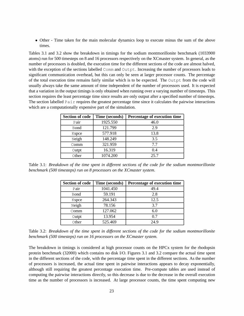
Tables 3.1 and 3.2 show the breakdown in timings for the sodium montmorillonite benchmark (1033900atoms) run for 500 timesteps on 8 and 16 processors respectively on the XCmaster system. In general, as thenumber of processors is doubled, the execution time for the different sections of the code are almost halved,with the exception of the sections labelled Comm and Outpt. Increasing the number of processors leads tosignificant communication overhead, but this can only be seen at larger processor counts. The percentageof the total execution time remains fairly similar which is to be expected. The Outpt from the code willusually always take the same amount of time independent of the number of processors used. It is expectedthat a variation in the output timings is only obtained when running over a varying number of timesteps. Thissection requires the least percentage time since results are only output after a specified number of timesteps.The section labelled Pair requires the greatest percentage time since it calculates the pairwise interactionswhich are a computationally expensive part of the simulation.
Section of code Time (seconds) Percentage of execution timePair 1925.550 46.0Bond 121.799 2.9Kspce 577.918 13.8Neigh 148.249 3.5Comm 321.959 7.7Outpt 16.319 0.4Other 1074.200 25.7
Table 3.1: Breakdown of the time spent in different sections of the code for the sodium montmorillonitebenchmark (500 timesteps) run on 8 processors on the XCmaster system.
Section of code Time (seconds) Percentage of execution timePair 1041.450 49.4Bond 59.191 2.8Kspce 264.343 12.5Neigh 78.156 3.7Comm 127.062 6.0Outpt 13.954 0.7Other 525.469 24.9
Table 3.2: Breakdown of the time spent in different sections of the code for the sodium montmorillonitebenchmark (500 timesteps) run on 16 processors on the XCmaster system.
The breakdown in timings is considered at high processor counts on the HPCx system for the rhodopsinprotein benchmark (32000) which contains no disk I/O. Figures 3.1 and 3.2 compare the actual time spentin the different sections of the code, with the percentage time spent in the different sections. As the numberof processors is increased, the actual time spent in pairwise interactions appears to decay exponentially,although still requiring the greatest percentage execution time. Pre-compute tables are used instead ofcomputing the pairwise interactions directly, so this decrease is due to the decrease in the overall executiontime as the number of processors is increased. At large processor counts, the time spent computing new
23
neighbour lists becomes more significant, as it is time consuming for an atom to locate its nearest neighbour.The time spent outputing data is almost negligible.
From Figure 3.2, the overall percentage time spent in communications increases with processor count. Forhigh processor counts, i.e. > 32, all communications take place across a switch, which leads to communica-tion overheads, which are greater for larger numbers of processors.
The next section discusses the actual benchmarking results obtained on each system.
24
Figure 3.1: Comparison of the actual time spent in different sections of the code on HPCx for the rhodopsinbenchmark (32000 atoms) with varying numbers of processors.
Figure 3.2: Comparison of the percentage time spent in different sections of the code on HPCx for therhodopsin benchmark (32000 atoms) with varying numbers of processors.
25
3.4 Benchmarking results
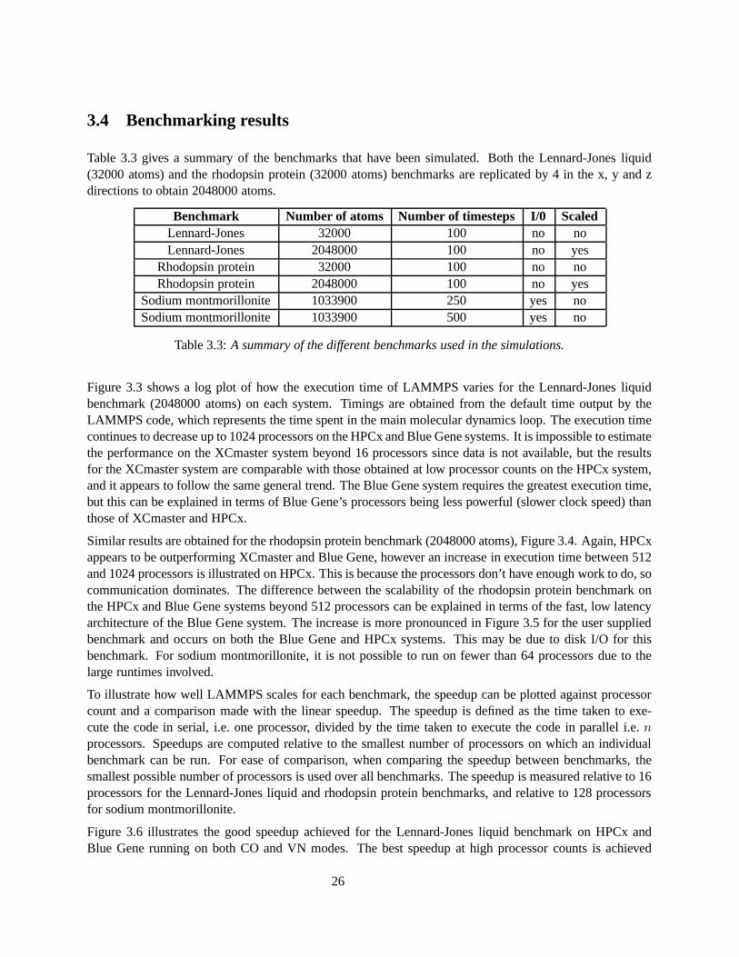
Table 3.3 gives a summary of the benchmarks that have been simulated. Both the Lennard-Jones liquid(32000 atoms) and the rhodopsin protein (32000 atoms) benchmarks are replicated by 4 in the x, y and zdirections to obtain 2048000 atoms.
Benchmark Number of atoms Number of timesteps I/0 ScaledLennard-Jones 32000 100 no noLennard-Jones 2048000 100 no yes
Rhodopsin protein 32000 100 no noRhodopsin protein 2048000 100 no yes
Table 3.3: A summary of the different benchmarks used in the simulations.
Figure 3.3 shows a log plot of how the execution time of LAMMPS varies for the Lennard-Jones liquidbenchmark (2048000 atoms) on each system. Timings are obtained from the default time output by theLAMMPS code, which represents the time spent in the main molecular dynamics loop. The execution timecontinues to decrease up to 1024 processors on the HPCx and Blue Gene systems. It is impossible to estimatethe performance on the XCmaster system beyond 16 processors since data is not available, but the resultsfor the XCmaster system are comparable with those obtained at low processor counts on the HPCx system,and it appears to follow the same general trend. The Blue Gene system requires the greatest execution time,but this can be explained in terms of Blue Gene’s processors being less powerful (slower clock speed) thanthose of XCmaster and HPCx.
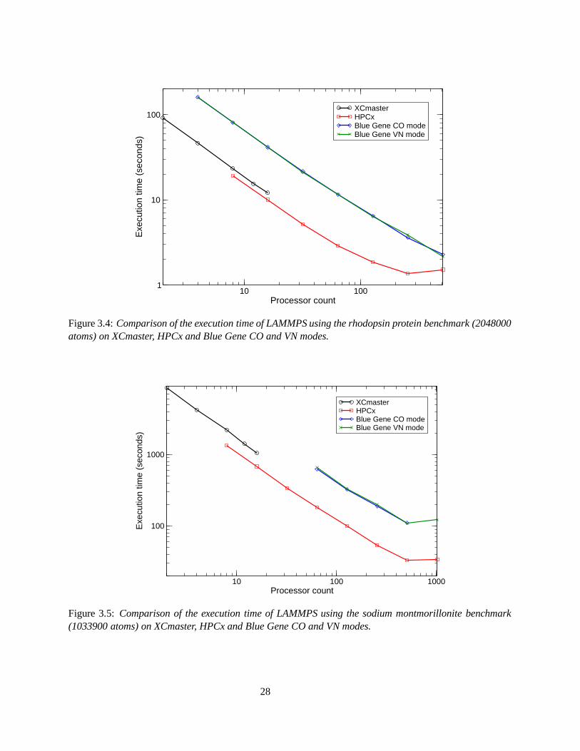
Similar results are obtained for the rhodopsin protein benchmark (2048000 atoms), Figure 3.4. Again, HPCxappears to be outperforming XCmaster and Blue Gene, however an increase in execution time between 512and 1024 processors is illustrated on HPCx. This is because the processors don’t have enough work to do, socommunication dominates. The difference between the scalability of the rhodopsin protein benchmark onthe HPCx and Blue Gene systems beyond 512 processors can be explained in terms of the fast, low latencyarchitecture of the Blue Gene system. The increase is more pronounced in Figure 3.5 for the user suppliedbenchmark and occurs on both the Blue Gene and HPCx systems. This may be due to disk I/O for thisbenchmark. For sodium montmorillonite, it is not possible to run on fewer than 64 processors due to thelarge runtimes involved.
To illustrate how well LAMMPS scales for each benchmark, the speedup can be plotted against processorcount and a comparison made with the linear speedup. The speedup is defined as the time taken to exe-cute the code in serial, i.e. one processor, divided by the time taken to execute the code in parallel i.e. nprocessors. Speedups are computed relative to the smallest number of processors on which an individualbenchmark can be run. For ease of comparison, when comparing the speedup between benchmarks, thesmallest possible number of processors is used over all benchmarks. The speedup is measured relative to 16processors for the Lennard-Jones liquid and rhodopsin protein benchmarks, and relative to 128 processorsfor sodium montmorillonite.
Figure 3.6 illustrates the good speedup achieved for the Lennard-Jones liquid benchmark on HPCx andBlue Gene running on both CO and VN modes. The best speedup at high processor counts is achieved
26
on the Blue Gene system in CO mode. As already mentioned, the Lennard-Jones liquid benchmark scaleswell to 1024 processors, and the design of Blue Gene is ideal for such applications. This benchmark hasdifferent interactions to the rhodopsin protein benchmark, i.e. it has no FFTW or PPPM, which means thatinteractions are short range, and communication only takes place with nearest neighbours. This behaviour isalso illustrated in Figure 3.7, which shows the speedup of the rhodopsin protein benchmark (32000 atoms)on HPCx and Blue Gene CO and VN modes. For low processor counts, CO mode appears to give betterperformance than VN mode, but a cross over point around 375 processors is reached where the speedup inVN mode overtakes that of CO mode.
The speedup of sodium montmorillonite benchmark in comparison to the ideal speedup is relatively poor onboth systems, Figure 3.8. On HPCx, the speedup begins to tail off after 256 processors and on Blue Geneafter 512 processors. Again, this is most likely due to large amounts of I/O involved and the communicationsrequired for the I/O.
Often the speedup of a code may be affected by the number of atoms used in the simulation. Figure 3.9shows that the speedup of LAMMPS generally increases with increasing numbers of atoms. By comparingthe rhodopsin protein benchmark run with 32000 atoms and 2048000 atoms, the speedup at 256 processorshas doubled. Increasing the number of atoms both increases the speedup and the scalability of the code.This is due to the change in ratio of computational work per processor versus communication overheadswith increasing problem size, i.e. processors have more work to do before communication is required.
10 100 1000Processor count
1
10
100
Exe
cutio
n tim
e (s
econ
ds)
XCmasterHPCxBlue Gene CO modeBlue Gene VN mode
Figure 3.3: Comparison of the execution time of LAMMPS using the Lennard-Jones liquid benchmark(2048000 atoms) on XCmaster, HPCx and Blue Gene CO and VN modes.
27
10 100Processor count
1
10
100
Exe
cutio
n tim
e (s
econ
ds)
XCmasterHPCxBlue Gene CO modeBlue Gene VN mode
Figure 3.4: Comparison of the execution time of LAMMPS using the rhodopsin protein benchmark (2048000atoms) on XCmaster, HPCx and Blue Gene CO and VN modes.
10 100 1000Processor count
100
1000
Exe
cutio
n tim
e (s
econ
ds)
XCmasterHPCxBlue Gene CO modeBlue Gene VN mode
Figure 3.5: Comparison of the execution time of LAMMPS using the sodium montmorillonite benchmark(1033900 atoms) on XCmaster, HPCx and Blue Gene CO and VN modes.
28
100 200 300 400 500Processor count
100
200
300
400
500
Spe
edup
Linear speedupHPCxBlue Gene CO modeBlue Gene VN mode
Figure 3.6: Comparison of the speedup of LAMMPS for the Lennard-Jones liquid benchmark (2048000atoms) relative to 16 processors on the HPCx and Blue Gene CO and VN mode systems. The linear speedupis denoted by the dashed line.
0 100 200 300 400 500Processor count
0
100
200
300
400
500
Spe
edup
Linear speedupHPCxBlue Gene CO modeBlue Gene VN mode
Figure 3.7: Comparison of the speedup of the rhodopsin protein benchmark (32000 atoms) relative to 16processors on the XCmaster, HPCx and Blue Gene CO and VN mode systems. The linear speedup is denotedby the dashed line.
29
0 200 400 600 800 1000Processor count
0
200
400
600
800
1000
Spe
edup
Linear speedupHPCxBlue Gene VN mode
Figure 3.8: Comparison of the speedup of the sodium montmorillonite benchmark (1039900 atoms) relativeto 128 processors on the HPCx and Blue Gene VN mode systems. The linear speedup is denoted by thedashed line.
0 200 400 600 800 1000Processor count
0
200
400
600
800
1000
Spe
edup
Linear speedupRhodopsin protein (32000 atoms)Rhodopsin protein (2048000 atoms)Lennard-Jones liquid (2048000 atoms)Sodium montmorillonite (1033900 atoms)
Figure 3.9: The speedup (relative to 16 processors) of LAMMPS on the HPCx system. The linear speedupis denoted by the dashed line.
30
3.5 Performance per timestep
It is interesting to see how the amount of time taken per timestep varies over the entire simulation time.Previous studies have shown a variation in timings over the first hundred timesteps. The time taken for eachstep over all three systems were analysed. Figure 3.10 shows the results for the sodium montmorillonitebenchmark run over 500 timesteps on the XCmaster system. The results clearly showed that the performanceis fairly consistent at each timestep, with only a small deviation notable in the 250 and 500 timesteps, whena small amount of data is written to the output file.
0 50 100 150 200 250 300 350 400 450 500Step
0
25
50
75
100
125
150
175
200
Tim
e (s
econ
ds)
Figure 3.10: Comparison of the time taken per timestep using the sodium montmorillonite benchmark over500 steps on the XCmaster system.
Figures 3.11 and 3.12 show the performance of each of the benchmarks on the XCmaster and HPCx systemsrespectively. The performance is measured by the number of processors divided by timesteps per second.The performance of each of the benchmarks is generally very stable on the XCmaster system up to at least16 processors with almost perfect scaling. The exception to this is at 12 processors on XCmaster. Thiscan be explained in terms of processor counts. For the LAMMPS code, the choice of processor countdetermines the particular PPPM grid. Some processor counts give more efficient PPPM grids (essentiallywith FFT computations) than others. For large processor counts on the HPCx system (Figure 3.12), theLennard-Jones liquid benchmark (2048000 atoms) illustrates perfect scaling on up to 1024 processors. Forthe sodium montmorillonite benchmark (both 250 and 500 timesteps), the scaling begins to drop off beyond512 processors, while for the rhodopsin protein benchmark (32000 and 2048000 atoms), the scaling dropsoff beyond 256 processors.
31
2 4 6 8 10 12 14 16Processor count
0
20
40
60
80
100
120
140
160
180
200
Per
form
ance
(pr
oces
sor
coun
t/tim
este
ps p
er s
econ
d)Lennard-Jones liquid (2048000 atoms)Rhodopsin protein (32000 atoms)Rhodopsin protein (2048000 atoms)Sodium montmorillonite (1033900 atoms; 250 timesteps)Sodium montmorillonite (1033900 atoms; 500 timesteps)
Figure 3.11: The performance of LAMMPS on the XCmaster system for each of the 3 benchmarks.
200 400 600 800 1000Processor count
0
50
100
150
200
Per
form
ance
(pr
oces
sor
coun
t/tim
este
ps p
er s
econ
d)
Lennard-Jones liquid (2048000 atoms)Rhodopsin protein (32000 atoms)Rhodopsin protein (2048000 atoms)Sodium montmorillonite (1033900 atoms; 250 timesteps)Sodium montmorillonite (1033900 atoms; 500 timesteps)
Figure 3.12: The performance of LAMMPS on the HPCx system for each of the 3 benchmarks.
32
3.6 Intel MPI Benchmarks (IMB)
IMB3 (formerly known as Pallas MPI benchmarks) are an open source set of MPI benchmarks used toevaluate the combined performance of memory and interconnect. IMB measures performance over a widerange of message sizes, in an attempt to show the performance behaviour for small and large messages. Thebenchmarks are written in ANSI C using message passing paradigm and are targeted at measuring importantMPI functions, such as [21]:
• Point-to-point message passing,
• Global data movement and computation routines,
• One-sided communications, and
• File I/O.
Benchmark results can be obtained for a number of MPI communications. These include collective com-munications such as MPI_Allreduce, MPI_Allgather, MPI_Alltoall, MPI_Bcast and MPI_Barrier, as wellas point-to-point communications including MPI_Sendrecv, PingPong and PingPing. PingPong involvesMPI_Send and MPI_Recv directly between two processors, either over the switch or within a node viashared memory. PingPong is the classic way of measuring startup (latency) and throughput (bandwidth)of a single message sent between two processes. The communication bandwidth (measured in MBs) andlatency (measured in microseconds) of a particular parallel machine affects the efficiency of the machine.Lower latency implies a better and faster network and is critical for applications that exchange relativelyshort messages in real-time and are sensitive to message transmission delays [16].
In this project, we report on the performance results obtained on each of the three systems. Results fromthree IMB benchmarks are selected and presented to illustrate how communication varies on different sys-tems. These include MPI_Bcast, MPI_Allreduce and PingPong. MPI_Bcast broadcasts a message fromprocess with rank root to all other processes, while MPI_Allreduce combines values from all processes anddistributes the results back to all processes. These particular collective communications can be used to anal-yse the scalability of LAMMPS at high processor counts. The results from the IMB benchmarks give thebest possible communication between two processors. The switch communication should show insignificantdifference, since communications are via the same switch.
Figure 3.13 shows the bandwidth against message size for the PingPong benchmark on each system. Thehigher the line, the better the performance. As the message size is increased, the bandwidth on the HPCxsystem is significantly higher than that of XCmaster and Blue Gene, indicating that the HPCx system givesthe best performance for larger messages. This behaviour is illustrated in Figure 3.14, which shows the timetaken to exchange messages of varying sizes. In this case, the lower the line, the better the performance.Again HPCx exhibits the best performance closely followed by XCmaster. The Blue Gene system has thepoorest performance as the message size is increased.
Plots for the collective communication MPI_Allreduce against the number of processors is illustrated in Fig-ures 3.15 and 3.16 for low and high processor counts respectively, and a comparison is made with MPI_Bcastin Figure 3.17. Results are given for two different message sizes: 32 B and 32 KB, since LAMMPS involvesexchanging a large number of small messages and a large number of large messages. For both MPI_Bcastand MPI_Allreduce, the Blue Gene system appears to perform best for smaller messages and illustrates
3Downloaded from http://www.intel.com/software/products/cluster/downloads/mpi_benchmarks.htm
33
poorer performance for larger messages, while the HPCx shows the opposite behaviour, i.e. poor perfor-mance for small messages and good performance for larger messages.
Each of the three architectures exhibit the same behaviour as the number of processors is increased. Thesmaller the execution time for the MPI_Allreduce benchmark, the better performance. For large processorcounts the MPI_Allreduce benchmark gets significantly worse on HPCx and Blue Gene than for smallprocessor counts.
0 1e+06 2e+06 3e+06 4e+06Message size (bytes)
0
1000
2000
3000
4000
5000
6000
Ban
dwid
th (
Mby
tes/
seco
nd)
XCmasterHPCxBlue Gene
Figure 3.13: Variation of bandwidth with message size for the PingPong benchmark on the XCmaster, HPCxand Blue Gene systems.
34
0 1e+06 2e+06 3e+06 4e+06Message size (bytes)
0
5000
10000
15000
20000
25000
30000
Tim
e (m
icro
seco
nds)
XCmasterHPCxBlue Gene
Figure 3.14: Variation of time with message size for the PingPong benchmark on the XCmaster, HPCx andBlue Gene systems.
1 10Processor count
10
100
1000
t avg (
mic
rose
cond
s)
XCmasterHPCxBlue Gene
32 B
32 KB
Figure 3.15: Comparison of the time taken (at low processor counts) for the MPI_Allreduce benchmark withtwo different message sizes of 32 B and 32 KB on the XCmaster, HPCx and Blue Gene systems.
35
100 1000Processor count
10
100
1000
t avg (
mic
rose
cond
s)HPCxBlue Gene
32 B
32 KB
Figure 3.16: Comparison of the time taken (at high processor counts) for the MPI_Allreduce benchmarkwith two different message sizes of 32 B and 32 KB on the XCmaster, HPCx and Blue Gene systems.
1 10Processor count
1
10
100
1000
t avg (
mic
rose
cond
s)
XCmasterHPCxBlue Gene
32 B
32 KB
Figure 3.17: Comparison of the time taken (at low processor counts) for the MPI_Bcast benchmark withtwo different message sizes of 32 B and 32 KB on the XCmaster, HPCx and Blue Gene systems.
36
3.7 Reproducibility
All benchmark results are run multiple times and the smallest execution time is recorded. Any abnormalitiesin results have been run extra times to ensure they are accurate. For low processor counts, i.e. ≤ 256 pro-cessors, the timings obtained are generally very stable, with only a small difference between runs. For highprocessor counts, there is a notable difference in the timings obtained, but the overall percentage differenceremains small.
On each computer system, the benchmarks are run on a production system, which means that other users arerunning codes concurrently. This may limit the codes performance. Submitting jobs that require less than16 processors to the XCmaster system does not guarantee sole access to that node. Since the nodes operatewith shared memory within a node, on many occasions this was found to affect the overall runtime of thecode. Even submitting two jobs to the same node could increase the overall runtime by as much as 5%. Theonly way to guarantee access to the entire node is to request the use of all 16 processors but only run the jobon the required number of processors. This however, does not make efficient use of resources and delaysother users from running their code.
To ensure that any startup costs or instabilities are removed, each benchmark is run twice with a differentnumber of timesteps. Table 3.4 shows the percentage difference between the timings obtained when therhodopsin protein benchmark (32000 atoms) is run using 50 and 100 timesteps. The time obtained for the 50timestep run is subtracted from that of the 100 step run and compared with the 50 step run. The startup costsassociated with the rhodopsin protein benchmark are almost negligible since the input file data.rhodo issmall, i.e. 6 MB. Thus the cost per timestep for a 100 step run is almost identical for the 100-50 timesteprun. Due to the sodium montmorillonite benchmark requiring I/O, it was expected that the startup costsassociated with this benchmark would be significantly greater. However, as illustrated in Table 3.5, the onlymajor percentage difference was found for the 8 and 12 processor counts on the XCmaster system. Thismay be due to the particular PPPM grid used or perhaps another user is running a smaller processor job onthe same node.
Table 3.5: Startup costs of the sodium montmorillonite benchmark (1033900 atoms) on the XCmaster system.
37
3.8 32 processors on XCmaster
A request was made at the beginning of the project to set up a 32 processor queue on the XCmaster system.The queue was set up with 30 minutes of CPU time, and was only available for access by myself andFiona Reid. If the queue was successful and proved to work correctly, this time was to be increased toa number of hours and opened out to other users of the system. Initially the queue was tested using therhodopsin protein benchmark (32000 atoms). Table 3.6 shows the results obtained on 32 processors. Thereis a significant increase in execution time on the 32 processor queue. Other benchmarks were also testedand were found to significantly increase the execution time of LAMMPS. Since LAMMPS has been foundto scale well to a several hundred processors using these benchmarks, it was expected that the executiontime of LAMMPS should continue to decrease on 32 processors. It was suggested that the quadrics switchfor inter-node communication was not being used correctly, i.e. the default interconnect was not correct,so the interconnect was set by specifying "-elan -subnet 172.22.0.1" as options to mpirun in the batchsubmission script, where "subnet" conforms to the IP address of the quadrics subnet. Adding the "-prot"option showed that the nodes were over-subscribed, i.e. the code was not running on two nodes but thatall 32 tasks were running on a single 16 processor node. This suggests that the tasks are constantly beingswapped in between processors, which is why the runtime is so large. To verify that a single node is beingused the MPI_GET_PROCESSOR_NAME routine for a simple "Hello World" MPI code was tested, and thisverified that all tasks were being processed on a single node. The MPI_GET_PROCESSOR_NAME routineis part of the MPI standard and returns the name of the processor on which the task is run. In this case, all32 tasks were being run on the same node, i.e. node 9. An example of using this routine on the XCmastersystem is provided in Appendix A.
Processor count Execution time (seconds)2 96.9784 49.0278 24.628
12 16.68216 12.68732 78.499
Table 3.6: Results obtained from running LAMMPS on the "32 processor" queue on the XCmaster system.
A number of other suggestions were made:
1. Use the following on the bsub command line in the batch submission script:bsub -q 32cpus -R "span[ptile=16]" myjobThis is supposed to request 16 processors on each available host. The option "span[ptile=x]"is normally used with the resource to specify the number of core to use per compute node.
2. Run the IMB "PingPong" benchmark on all processor counts from 2 up to 32 processors.
3. Run using the newest MPI version HP MPI 02.02.00.00 Linux IA64, instead of version HP MPI02.01.01.00 Linux IA64.
Each of these suggestions were tested, but there were no significant changes in the execution time, and thesesuggestions further confirmed that the job was only being executed on a single node.
38
3.9 Simultaneous Multithreading (SMT) on HPCx
There are three main types of multithreading:
1. Coarse-grain - An instruction is executed on a single thread until the thread encounters a long latency,at which point the instruction is passed to another thread until it encounters a long latency and so on;
2. Fine-grain - Instructions are issued on each cycle by a single thread; and
3. Simultaneous Multithreading (SMT) - Two threads execute simultaneously on the same processor.
SMT aims to reduce the inefficiency caused by processors remaining idle over a large percentage of thetotal processor time of a particular code [15]. SMT works by allowing multiple threads to issue multipleinstructions at each cycle, thus attempting to improve the performance of the code. Figure 3.18 shows anexample of how SMT could work. Each box represents an issue slot. If the box is filled, the processorexecutes an instruction, and if the box is empty, the slot is unused. Each row represents a single executioncycle. Unused slots are characterised as horizontal waste, in which some (but not all) of the issue slots canbe used, and vertical waste, in which a cycle is completely unused. SMT processors select instructions fromany thread and dynamically schedules machine resources among the instructions, thus effectively utilisingthe available hardware.
Figure 3.18: (a) Superscalar multithreading; (b) Fine-grain multithreading (c) Simultaneous multithreading.Each box represents an issue slot. If the box is filled the processor executes an instruction, otherwise theslot is unused. Figure adapted from [22].
A comparison is made with and without the use of SMT on the HPCx system. The rhodopsin proteinbenchmark (32000 atoms) is chosen for this comparison. With SMT enabled, two tasks are allocated to eachprocessor. When SMT is not enabled the number of MPI tasks is equal to the number of processors on whichthe code is being run. Figure 3.19 shows that SMT significantly improves the performance of LAMMPS atlow processor counts by a factor of up to 1.1. As the number of processors is increased, a cross over point(at 320 processors) is reached, whereby, the addition of SMT now reduces the performance of the code, andthe code performs better when SMT is not enabled. This can be explained in terms of the scalability of thecode. Recalling Figure 3.9 which illustrates the poor speedup achieved from this benchmark as the numberof processors is increased. With SMT enabled, there are double the number of tasks than when SMT is not
39
enabled. Therefore, any communication bottlenecks between these tasks are encountered at low processorcounts.
POWER5 processors have two floating point units and support SMT with two threads. Therefore, havingtwo virtual processes running per physical processor.
The main drawback with enabling SMT is that there is increased communication, and the memory limit pertask is halved. No difference is observed in memory bandwidth. Caches are effectively halved in size, thusany improvement in applications is due to reduced memory latency.
Tables 3.7 and 3.8 give the percentage improvement in the execution time of the sodium montmorillonite(1033900 atoms) and Lennard-Jones liquid (2048000 atoms) benchmarks respectively. The greatest im-provement over all benchmarks was in the user supplied benchmark. This may be because the user suppliedbenchmark is a much larger benchmark than the rhodopsin protein and Lennard-Jones liquid benchmarks.Also, the user supplied benchmark contains a significant amount of I/O, whereas the benchmarks suppliedwith the LAMMPS code simply have to read in initial data files. It was found that I/O takes the same amountof time regardless of the number of processors being used. This suggests that I/O is essentially a serial partof the code. The I/O associated with the user supplied benchmark is less than expected for benchmarks ofthis type, since it only dumps the atoms position out to file and not the velocity of the atoms or the forcesacting on the atoms.
Overall, the rhodopsin protein benchmark gave an improvement factor of 1.36, while the Lennard-Jonesliquid and sodium montmorillonite benchmarks improved by a factor of 1.1 and 2.28 respectively. Theseresults are broadly comparable with results obtained from other classical molecular dynamics codes whichhave been found to improve by a factor of 1.4 [15].
40
0 100 200 300 400 500Processor count
0
100
200
300
400
500
Spe
edup
Linear speedupWithout SMTWith SMT
Figure 3.19: Comparison of the speedup of the rhodopsin protein benchmark (32000 atoms) with and with-out SMT enabled. A cross over point is reached at 320 processors. For less than 320 processors SMT is foundto improve performance, whereas for greater than 320 processors SMT is found to degrade performance.
Processor count Time (seconds) With SMT PercentageWithout SMT With SMT improvement
Table 3.8: Comparison of the timings obtained for the Lennard-Jones liquid benchmark (2048000 atoms)with and without SMT on the HPCx system.
41
3.10 Summary
A number of results have been presented and analysed. HPCx appears to give the best performance, closelyfollowed by XCmaster (at low processor counts) and then Blue Gene. Blue Gene on the other hand offersmuch better scaling to large numbers of processors than HPCx or XCmaster. The best scaling is found forthe benchmarks supplied with the LAMMPS code, since they do not contain any disk I/O. The scalability ofthe code can be improved by increasing the problem size. The results obtained have been run a number oftimes and are fully reproducible on all three systems.
Results from the IMB benchmarks illustrate that the Blue Gene system exhibits the best performance forsmall messages, while HPCx exhibits the best performance for large messages. Increasing the number ofprocessors reduces the performance of the Intel MPI_Allreduce benchmark. Enabling SMT is found toimprove the performance by a factor of at least 1.1 for the benchmarks supplied with the code, and at least2.28 for the user supplied benchmark.
According to the LAMMPS output file, the section of code that requires the most execution time is in thecalculation of pairwise interactions. To verify that the output from LAMMPS is correct, profiling is used toidentify the most computationally expensive components of the code.
The next chapter presents results from profiling both the serial and parallel version of LAMMPS on eachsystem.
42
Chapter 4
Profiling and performance analysis
Profiling allows us to identify which sections of a code are taking the longest time to execute and hencelimiting the codes performance. It helps to identify the parts of the code which are potential candidatesfor code optimisation. It is a relatively difficult process, as it involves using a wide range of profilingtools to identify the sections of code that are taking the longest time to execute, and also those that makeinefficient use of the architecture on which the code is run. Identifying the methods with the longest runtimeis not always straightforward. It involves learning how to use the different profiling tools available on eachmachine.
There are many reasons for carrying out performance analysis. The main objectives are usually to reducethe total execution time of the code and also to achieve good scaling to large numbers of processors. Whenprofiling, it is often necessary to turn off all optimisations, as different levels of optimisation can reorder theinstructions when the code is compiled. This can result in the runtime of the code increasing significantly.However, if we want to be able to identify bottlenecks, this increase in runtime must be tolerated. The outputfrom the profiling results should be as close as possible to the source code, so that the exact location of thebottleneck can be found.
The serial version of LAMMPS is used initially, as this avoids complication of which processes are runningwhich parts of the code. It is possible that amendments to the code may change the order in which messagesare passed or even the number of times a certain MPI routine needs to be called. Once the serial version hassuccessfully been profiled and optimised, the parallel version of the code is considered.
Also, LAMMPS 2006 has not been previously profiled on XCmaster, HPCx and Blue Gene/L system, sounderstanding the computationally expensive parts of the code is important. There are two aspects of thecode that are considered:
1. Serial performance on all three systems.
2. Scaling at large processor counts on HPCx.
4.1 Profiling tools
Performance tools are very useful for large scaled applications. They enable code to be examined for per-formance and memory usage problems. Trace data shows how much processor time each part of the code
43
uses. It records information about different events, without requiring any code instrumentation overhead.Compiling with a debugging flag (often required for profiling) can increase the total execution time of thecode.
Traditional profiling tools such as prof and gprof are standard tools used for simple or quick performanceanalysis. Both tools time programs at method or function level and obtain data to analyse the codes’ per-formance. prof is used to generate a statistical program profile (called a flat profile) of the amount of CPUtime used by a program, together with the number of times each method within the main program has beencalled, and the percentage of the total execution time spent in each method. In addition to this flat profile,gprof, which is used to produce a call graph profile, counts the number of times each caller-callee pair istraversed in the program’s call graph. This allows for a more detailed analysis to be carried out.
Since both these tools are standard UNIX commands, they are available on all three systems. However,they are not fully supported by the Intel compilers on XCmaster. To run prof and gprof on HPCx and BlueGene requires compiling and linking with the -g and -pg debug flags respectively, at compile time, andthen run the code as usual to produce a profile data file (gmon.out). Intel compilers specify that the codemust be compiled and linked with -p and -g flags. However, this still does not guarantee that call graphinformation is produced. Unfortunately, when run with the LAMMPS serial version of the code, no timingis accumulated, only the number of times each method is called can be obtained on the XCmaster system.
The main drawback with prof and gprof is that they only provide information on the CPU usage, there is noanalysis of I/O or communications, and thus this may only be used for analysis of serial code.
The profiling tools that are available on each system are discussed in the following sections.
4.2 XCmaster
A Trace Collector library is installed on the XCmaster, which allows us to create, sort and display tracedata to evaluate the impact of MPI communications on an application. A Trace Analyzer library is alsoavailable to view the trace files, in an attempt to understand the communications patterns and potentialsources of performance bottlenecks. These tools will only work with Intel compilers. Both of these toolsform part of the Intel Cluster Tools (ICT). The Trace Collector may be used to trace MPI routines, user codeand library routines. The Trace Analyzer is a GUI based tool, which uses timelines and parallelism displaysto visualise the concurrent behaviour and calculate statistics for specific time intervals and processes [23].Statistical data is provided in a combination of function, message and collective operation profiles, andcommunication statistics can be viewed over an arbitrary time interval.
To use these tools, the Intel Trace Collector library must be linked at compile time, such that the GNUMakefile is as follows:
CC = mpiiccIFLAGS = -I/genusers/geraldine/fftw-2.1.5/include -DFFT_FFTW \
The default points to the most recently installed versions of Trace Collector and Analyzer, which are cur-rently not working correctly on the system. However, it is still possible to use the older version of thesetools which have been previously installed. The low overhead associated with using these tools ensures theruntime remains unaltered. However, it is still necessary to insert timers into the code to measure the amountof time spent in a particular method, since these profiling tools can only evaluate the amount of time spentin MPI communications.
XCmaster also uses VTune to analyse the performance of shared memory programs [24]. This can also beused to indicate the amount of time spent in particular methods within an MPI program. Unfortunately, todo this, VTune must be run interactively, and so the results may not be very reliable as the master process isbeing shared by many users. For this reason, VTune is not used in this investigation.
4.3 Blue Gene
The Blue Gene system uses MPI Tracer and MPI Profiler, each consisting of a set of libraries. MPI Traceridentifies performance bottlenecks and relates these back to the source code. MPI Profiler collects an overallsummary of calls made to a method. MPI Profiler is a more advanced version of MPI Trace. It uses Peekperfto visualise the communication statistics, and maps the collected data back to the source code, making iteasier for the user to identify the potential bottlenecks. PeekPerf is a suitable tool for investigating thescalability of the code. To use MPI Profiler, it is necessary to compile with the -g debug flag and link withthe lmpitrace_c library as before. The code is then executed as before and .viz files are produced.These are then viewed using Peekperf.
Blue Gene also uses Xprofiler, which is a simple profiling tool used to analyse the performance of bothserial and parallel codes at source level. Similar to prof and gprof, it only profiles CPU usage and doesnot give any indication of the amount of I/O or number of communications. It does however, identify thecomponent of the code that takes the largest amount of time and uses a GUI to display the output of theprofiling. It does this by producing a flat profile and from this, a particular method can be selected and ahistogram produced, which can be displayed along with the source code. The histogram uses tick countsas a generic way of counting time. Each tick is equivalent to 0.01 seconds of CPU time. Thus, the moreticks accumulated, the more time is spent in that particular section of the method. In addition to the standard
45
techniques, Xprofiler allows methods which are initially grouped by libraries to be filtered and all librarycalls can be hidden. To use Xprofiler, the code must be linked with the lapack library, and run in the ususalway. Each process then writes an additional file to disk containing the profiling data.
function_trace is a feature of MPI Tracer which details the amount of time spent in different methods withinthe code, thus enabling the most computationally expensive sections of the code to be determined. To usefunction_trace, the application code must be linked with the lmpitrace_c library:
-L/bgl/local/lib/mpitrace -lmpitrace_c
and compiled using -qdebug=function_trace.
To run the code, the environment variable
-env "FLAT_PROFILE=yes"
must be set in order to obtain a breakdown of the total time spent in each method.
4.4 HPCx
HPCx uses a highly portable tool called VAMPIR (Visualisation and Analysis of MPI Resources) to providea better understanding of the communications that take place in an MPI code [25]. It analyses the messageevents where data is transmitted between processors. Data is presented in graphical form, i.e. tracefiles,allowing us to visualise the communication patterns, as well as providing detailed information on timingstatistics, event ordering and message sizes. Timelines are used to display the code execution and timingsstatistics, whereas activity charts are used to present per-process profiling information. To use VAMPIR anumber of paths must be set in both the LoadLeveler script and the interactive shell.
To allow 64-bit addressing, the code must be linked with:
-L$(PAL_ROOT)/lib54 -lVT -lld .
A more useful tool for MPI profiling (particularly for large numbers of processors) is the IBM tool MPI-Trace, which summarises the amount of time the code spends in communication routines. This includes thenumber of times a particular MPI routine is called, the average message size for that routine and the timespent in each MPI routine. To use MPITrace, a special mpitrace library must be linked at compile time.
HPCx also uses Xprofiler, similar to that available on the Blue Gene system.
4.5 Profiling overheads
Performance profiling often generates overheads during the execution of the code. This overhead is calcu-lated by the increase observed in the execution time when profiling is introduced to the code relative to theexecution time observed without profiling. In complex codes it is not unusual for the runtime to increase byas much as ten times when profiling is invoked. Results for the LAMMPS code are given in Section 4.9.
46
4.6 Correctness
To verify the correctness of the results obtained from the profiling tools and also to get more detailed in-formation of the time spent within each method, a number of timers can be used. For the serial versionof LAMMPS, the gettimeofday() function is available on all three systems. gettimeofday() provides wallclock time and can be used to find the elapsed time of a certain section of code, or even measure the timetaken by an entire method. Since there are no profiling tools available on XCmaster to calculate the timespent in different methods, it is essential to insert timers around certain methods to ensure that the resultsare in good agreement with those obtained on the HPCx and Blue Gene systems. It is also useful to obtainthe time spent in specific sections in a method, for example, around an if block, as illustrated in Figure4.1. Here, the ifdef structure is used, which allows the timers to be switched on and off depending onwhether or not the section of code is to be timed. To switch the timers on, the -DCOUNTER_ON option mustbe specified at compilation. A header file must also be created, which includes all the necessary *.h filesrequired to use the gettimeofday() timer and all the variables that are used when the timer is invoked.
Another available timer for the MPI version of LAMMPS is MPI_WTime(), which returns a 64-bit floatingpoint number of seconds representing the elapsed wall-clock time from some time in the past. Since profilingonly provides method or routine level data, in order to optimise LAMMPS it is necessary to insert timingsaround specific blocks, similar to that of the serial timer gettimeofday().
Figure 4.1: An example of inserting the gettimeofday() timer around a specific if block in order toobtain the time spent in this part of the method.
47
4.7 Results from profiling the serial version of LAMMPS
By analysing the execution of the code, the sections where the majority of time is spent can be identified andit is these particular methods that are focused on when optimising the code. When profiling, the methodsthat require 5% or more of the total execution time are considered for optimisation. Profiling is performedwithout any optimisation flags so that individual lines referred to by the profiling tool are the same as thoseof the source code, i.e. re-ordering hasn’t taken place.
The majority of profiling has been carried out using the rhodopsin protein benchmark with 32000 atoms,since this is a stable benchmark and profiling results are available on each of the three systems. Problemswere encountered when trying to profile the serial version of LAMMPS using the user supplied benchmarkon the Blue Gene system, since the problem size is too large to fit into memory. An error message of thefollowing form was displayed in the error file:
Failed to allocate 74649600 bytes for array pppm:vg.Therefore attempting to profile/run the serial version of the sodium montmorillonite benchmark is not pos-sible on the Blue Gene system.
Class method Number of calls Percentage TimePair_LJ_Charmm_Coul_Long::compute() 101 59.9
Table 4.1: The results from the Xprofiler profiling tool on the HPCx system for the rhodopsin protein bench-mark (32000 atoms), detailing the class methods that take 5% or more of the total execution time, togetherwith the number of times each class method is called.
Table 4.1 illustrates the output of a section of the flat profile obtained using the Xprofiler tool on the HPCxsystem for the rhodopsin protein benchmark with 32000 atoms. The rest of the output is less significant(and has been omitted) as it does not affect the total execution time as much as these particular methods. Toensure that these results were correct, a comparison was made with the results obtained from the gprof tool,which showed negligible difference. gprof is useful in that it also calculates the overhead due to profilingusing a function called mcount. In this case it was found to have an overhead of 3.7% of the total executiontime.
Table 4.1 shows that the method Pair_LJ_Charmm_Coul_Long::compute() consumes almost 60%of the total execution time. In total, these four methods consume almost 82.5% of the total time and aretherefore good candidates for optimisation. Any optimisation performed within these methods should po-tentially give the greatest improvement in the overall performance of the code. Optimisations made to othermethods should not substantially affect the performance of the code. The number of times the methodNeighbor::find_special() is called is a significant overhead in itself.
The Xprofiler and gprof tools invoked on Blue Gene also identified the same four methods. Results areavailable in Appendix B, Table B.1 for further reference.
48
Table 4.2 shows the results obtained from profiling the Lennard-Jones liquid benchmark with 2048000atoms on the Blue Gene system. Similar results are obtained on the HPCx system. In this case, the two mainmethods involved are Pair_LJ_Charmm_Coul_Long::compute() andNeigh_half::half_bin_newton(), consuming almost 95% of the total execution time. The othertwo methods mentioned previously for the rhodopsin protein benchmark are not called here and are thereforenot considered to be major bottlenecks when running the Lennard-Jones liquid benchmark.
Class method Count Time Percentage of(seconds) total time
Table 4.2: The results from the Xprofiler tool on the Blue Gene system for the Lennard-Jones liquid bench-mark (2048000 atoms).
On the XCmaster system, the gettimeofday() timer is used to time the four suggested methods to showthat the results are in good agreement with those obtained on the HPCx and Blue Gene systems. Table 4.3shows the results obtained for the rhodopsin protein benchmark with 32000 atoms. These four methodsin total consume 91.2% of the total execution time, which is comparable with the total percentage timeconsumed on HPCx (82.4%) and Blue Gene (95.9%).
Class method Count Time Percentage of(seconds) total time
Table 4.3: The results from the gettimeofday() timer on the XCmaster system for the rhodopsin proteinbenchmark (32000 atoms).
To verify that the results obtained from the profiling tools on the HPCx and Blue Gene systems are correct, itwas also beneficial to insert timers around the four suggested methods on these systems. A variable countwas also initialised and on entering each method, was incremented to verify that the number of times eachmethod was entered is equal to the number of times the methods are called (from profiling), and thus thetimings obtained are reliable. For further reference see Appendix B, Tables B.2 and B.3.
4.8 Results from profiling the parallel version of LAMMPS
Although the gprof and Xprofiler tools facilitate good analysis of CPU usage, as mentioned previously, theydo not provide information on other types of profiling such as idle CPU usage, I/O or communications.
49
The following section uses the VAMPIR profiling tool to identify the communications that are taking placewithin LAMMPS.
4.8.1 Communications via VAMPIR
Figure 4.2 shows a graphical representation of the communication patterns occurring within LAMMPSon 16 processors for a single timestep run. Pre-defined activities are illustrated using a combination ofcolours and labels. MPI communications blocks are represented in red, user code is represented in greenand purple is reserved for MPI collective operations such as MPI_Allreduce. It should be noted that thisfigure illustrating the global (all processes 0-15) timeline has been zoomed to see a finer granularity in thetimeline display. Often the granularity is too coarse and the purple lines are most dominating. The blacklines represent communications between processes.
The time spent (for a single timestep) can be broken down into different sections (Figure 4.3). In the range0 - 0.95 seconds, data is initialised and read in from the input file. All processors must wait until the masterprocess finishes reading in the data. Once the master process finishes reading the data, it is then distributedto all processors using MPI_Bcast. From 0.95 - 2.02 seconds, time is spent communciating in MPI_Send,MPI_Irecv, MPI_SendRecv and MPI_Wait. The range 2.02 - 2.36 seconds focuses on the main moleculardynamics computation. The final range 2.36 - 2.394 seconds involves freeing communicators, gatheringresults and outputting timings to file/screen.
The Activity Chart supplied in the VAMPIR analysis shows that all processes have balanced workload,i.e. similar amounts of serial code execution and similar amounts of MPI communications.
50
Figure 4.2: VAMPIR analysis of a single timestep for the rhodopsin protein benchmark (32000 atoms) runon 16 processors on the HPCx system. The timeline has been zoomed in the range 2.381 - 2.383 seconds.
Figure 4.3: VAMPIR analysis of a single timestep for rhodopsin protein benchmark (32000 atoms) run on16 processors on the HPCx system. The timeline is an overview of the whole run.
51
4.8.2 Communications via MPITrace
Table 4.4 shows a comparison of the amount of time spent in different MPI communications when thenumber of processors is increased from 16 to 128. Profiling is performed using the rhodopsin proteinbenchmark with 32000 atoms on the HPCx system. As the table suggests, there is no time associated withcalls to MPI_Barrier. Examination of the source code reveals that the major classes from which MPI_Bcastis called are read_data.cpp and read_restart.cpp, with calls from many other classes too. Bothof these classes are associated with the initialisation stages of the code. MPI_Allreduce, is also calledthroughout the code, with the majority of calls from the classes finish.cpp and fix_shake.cpp.These classes are associated with the collection of data from all processes at the end of each timestep.Other MPI calls are made to MPI_Send, MPI_Irecv, MPI_Sendrecv and MPI_Wait, none of which areassociated with the initialisation stages, but instead are probably associated with communications betweenprocesses at the end of each timestep. MPI_Wait is called from the classes: comm.cpp, dump.cpp,fix_shake.cpp, pppm.cpp, remap.cpp, special.cpp and write_restart.cpp.
MPI Routine Time (seconds) Time (seconds)16 processors 128 processors
Table 4.4: Comparison of the amount of time spent in different MPI routines (obtained using the MPITraceprofiling tool) for the rhodopsin protein benchmark (32000 atoms) run on 16 and 128 processors on HPCx.
Figure 4.4 shows the average amount of time spent in different MPI communication routines against proces-sor count on the HPCx system. For large processor counts, communications contribute significantly to theperformance of the code. The five major time consuming routines are MPI_Send, MPI_Wait, MPI_Waitany,MPI_Bcast and MPI_Allreduce. In particular, for a 128 processor count, MPI_Allreduce is dominating,while for a 1024 processor count MPI_Bcast is most dominating.
4.8.3 Communications via Trace Collector and Trace Analyzer
Figure 4.5 shows a comparison of the amount of time spent in different MPI routines for an 8 and 16 proces-sor count on the XCmaster system. The two dominating MPI routines are MPI_Bcast and MPI_Allreduce.Comparing MPI_Bcast on 8 processors with MPI_Bcast on 16 processors shows doubling of the time spentin this MPI routine. This is to be expected as there are twice as many processors to broadcast the results to.
52
Figure 4.4: Comparison of the amount of time spent in different MPI routines (obtained using the MPITraceprofiling tool) for the rhodopsin protein benchmark (2048000 atoms) for large processor counts on HPCx.
Other MPI routines where time is spent are:
• MPI_Wtime, which outputs the elapsed time. Calls are made from the classes pppm.cpp andtimer.cpp.
• MPI_Finalise, which terminates the MPI execution environment.
• MPI_comm_dup which duplicates an existing communicator and all its cached information. This iscalled once from the class remap.cpp.
Figure 4.6 compares the time spent in different MPI routines between the HPCx and Blue Gene systems forthe rhodopsin protein benchmark (32000 atoms) run on 16 processors. For the Blue Gene system, MPI_Sendand MPI_Bcast are most dominating, while on the HPCx system, the greatest proportion of time is spentin MPI_Send and MPI_Allreduce. These differences may be due to the different architectures of the twomachines. i.e. HPCx is shared memory, while Blue Gene is distributed memory.
53
Figure 4.5: Comparison of the amount of time spent in different MPI routines (obtained using the TraceCollector and Analyzer tools) on XCmaster for the rhodopsin protein benchmark (32000 atoms) run on 8and 16 processors.
Figure 4.6: Comparison of the amount of time spent in different MPI routines (obtained using the MPITraceand MPI Tracer profiling tools) on the HPCx and Blue Gene systems for the rhodopsin protein benchmark(32000 atoms) run on 16 processors.
54
4.8.4 Communication time per processor
The MPI Tracer tool on Blue Gene can be used to illustrate the variation in the communication time oneach processor. Figure 4.7 shows that the communication time varies between approximately 3 - 13 secondsduring the simulation, and that some processors spend more time communicating than others.
0 1 2 3 4 5 6 7 8 9 10 11 12 13 14 15Processor ID
0
2
4
6
8
10
12
14
16
Com
mun
icat
ion
time
(sec
onds
)
Figure 4.7: The results from the MPI Tracer profiling tool on Blue Gene showing how the amount of com-munication time varies per processor.
4.9 Statistical inaccuracies
The figures provided from profiling tools may be inaccurate. For example, the results from a gprof analysisare based on a sampling process. The number of calls to a particular method, however, is an integer countand is therefore accurate.
There are a number of ways to reduce the inaccuracies caused by profiling tools. For example to eliminateerrors using the gprof tool, it is necessary to run the code several times and combine the output into asingle call graph profile. Other tools may not be so straightforward. It is therefore necessary to calculatethe overheads, i.e. the approximate percentage errors introduced when profiling. To calculate the overheadusing Xprofiler, the code was run using the same benchmark with no optimisation, and the difference withand without the addition of profiling flags are compared. Results are given in Table 4.5. This shows that theprofiling tools used for parallel performance analysis introduce the most significant overheads.
55
System Profiling tool/timer Percentage ErrorXCmaster Trace Collector/Analyzer 0.2
gettimeofday() 1.5HPCx gprof 3.4
Xprofiler 0.1VAMPIR 11.8MPITrace 2.7
gettimeofday() 2.2Blue Gene gprof 1.8
MPI Tracer 62.7MPI Profiler 65.4
function_trace 81.2gettimeofday() 2.9
Table 4.5: The overheads associated with using different profiling tools/timers on the XCmaster, HPCx andBlue Gene systems.
4.10 Summary
A number of profiling tools are available on each system to analyse the performance of the LAMMPS codeand to identify the major bottlenecks in the code. Each tool offers its own functionality, and is either aimedat profiling the serial version of the code or profiling the parallel version. Results from profiling the serialversion of the code on HPCx and Blue Gene identified four main routines as limiting the codes performance.As the XCmaster system does not have reliable profiling tools, timers are inserted into the code. The resultsfrom the profiling tools used on the HPCx and Blue Gene systems are also verified by inserting timers intothe major routines.
Profiling the parallel version of the code identified the MPI routines: MPI_Send, MPI_Wait, MPI_Bcast andMPI_Allreduce as contributing significantly to the execution time of the code. As the number of processorsis increased, communication appears to be the major bottleneck in the code.
The next chapter looks at a number of methods used to optimise C++ codes. It describes in detail therecommended optimisations for each of the four main methods identified from profiling.
56
Chapter 5
Optimising LAMMPS on XCmaster
There are two main optimisation techniques that may be considered to improve the runtime of a code. Thefirst involves basic optimisations such as adding compiler flags, which must be done by explicitly declaringthe compiler flags at compile and link time. The main drawback of using optimisation flags is that theymay increase compilation time. Also, the addition of optimisation flags may give wrong results as certaincalculations need to occur in a specified order. When no compiler flags are used, the compiler aims to reducethe cost of optimisation and at the same time makes debugging produce the expected result. This type ofoptimisation has already been discussed in Section 2.3.3.
The second form of optimisation is code optimisation, which involves changing the source code in an attemptto reduce the overall execution time. Some code optimisations may significantly improve the execution timewhile others may have a negative impact on the execution time. The only way to find out is to test each typeof optimisation and see how it affects the execution time of the code. A good compiler can automaticallyperform code optimisations such as aligning data, inlining methods and loop unrolling.
There are two main goals when optimising code:
1. Optimise for time efficiency, i.e. reduce the overall runtime of the code; and
2. Optimise for memory conservation. For example, reduce memory accesses such as unnecessarypointer chasing, unnecessary temporary arrays or tables of values that are cheap to recalculate. Ideallyall variables and arrays should be stored in the fastest possible memory, preferably registers, but thisis not always possible.
5.1 Possible optimisations
A number of optimisations are possible:
• Loop fusion - involves combining loops in an attempt to reduce loop overhead and allows for betterinstruction overhead. This can be done if the loops share the same iteration space.
• Loop unrolling - involves reducing the number of overhead instructions the computer has to executein the loop (by a factor equal to the unrolling depth). Fewer instructions means the probability of thevalue already being in cache is greater, therefore improving the cache hit rate.
57
• Using dynamic arrays (as opposed to static) - dynamic arrays mean the size of the array can bedetermined at runtime and is then used to reserve space, which defers setting the size of the arrayuntil program runtime, thus keeping memory usage to a minimum. Static arrays are declared prior toruntime and are reserved in stack memory.
• Store arrays in row-major order for C++ programs (column-major order for Fortran programs) -allows arrays to be accessed contiguously in memory, thus reducing the number of cache misses.
• Avoid redundancies - by storing and reusing results that have been computed previously, instead ofrecomputing them.
• Declare local variables in the inner most scope - this reduces the overhead incurred creating objectswhen the method is called and keeps variables as close to registers as possible.
• Where possible, multiply instead of divide - if possible compute R = 1/constant, then its almostalways faster to use x ∗ R instead of x/constant.
• Padding arrays - involves adding additional unused space between dimensions of arrays. This at-tempts to reduce cache misses due to set associativity1 in arrays.
• Re-ordering if statements - if it is found that one if statement is being executed more times thananother, then this if statement should be placed first such that fewer negative conditions are beingtested. Re-ordering if statements has no implications on the output of the program.
• Move calculations out of a loop.
• Faster for loops - if the order of the for loop does not contribute to the final result of the calculation,it is faster to count down to zero than it is to calculate the value of (max indice - indice), check if theresult is non-zero and if it is, increment the index and if not continue.
Each of the four class methods identified in Chapter 4 are individually examined. The main bottleneck thatfrequently occurred in these particular methods were if blocks executed inside for loops. In some cases itis relatively straightforward to do this even if the calculation is dependent on the loop indice. The followingexample illustrates how this can be achieved:
for (i = 1; i <= k; i++) {if (i < j) {...<code1>;...
}else {...<code2>;...
}}
becomes1set associativity - association of memory location with a set of cache lines.
58
for (i = 1; i <= j; i++) {...
<code1>;...
}for (i = j+1; i <= k; i++) {
...<code2>;
...}
However, when the condition of the if block depends on an array which has previously been defined usingthe for loop indice, this is not possible. Each of the above optimisations are considered when optimisingthe four main methods. Any changes to the methods are discussed in the following sections. It is importantto note that any changes made to the code allows for the same functionality, and produces the same floatingpoint results obtained prior to optimisation.
5.2 Optimising the method pair_lj_charmm_coul_long::compute()
Most of the computational effort is spent in the calculation of the forces acting on the atoms. A full forceevaluation requires 1
2N(N−1) force calculations, where N is the number of particles in the simulation. Thismethod is used to compute the Lennard-Jones potential described in Equation (1.1). It uses a number ofconditional blocks to ensure that calculations are taking place inside the cutoff radius. The method consistsof two for loops over all possible neighbouring atoms. Within this method, there are some unavoidablefunctions such as sqrt(r) (used in the polynomial approximation) and exp(r) which must be interpolated.Both these are computationally expensive functions and are necessary for the calculation of the forces andtherefore cannot be eliminated.
To investigate whether re-ordering of if conditions may be beneficial a "count" variable was created andinitialised to zero within this class method. This was incremented after each block of code, and was usedto determine whether a particular if condition is being executed a large number of times and thus limitingthe codes performance. In one instance it was found that the else part of an if...else statement wasbeing executed over 300 times more than the if part, and so it was sensible to re-arrange these blocks, suchthat the greatest workload was being executed first, i.e. the majority of conditions are true. The followingsnippet of code taken from the method pair_lj_charmm_coul_long::compute() illustrates thecode after the if and else blocks have been interchanged. The original code can be found in Appendix C.
Other possible optimisations within this section of code included removing a variable called erfc (high-lighted in the code above) from the else part of the if...else structure and substituting it into thevariable forcecoul. This allowed the variable expm2 to be factorised out, thus reducing the total num-ber of floating point operations.
Another optimisation involved declaring six new variables such that:dii = deli * delianddij = deli * deljwhere i and j denote the variables x, y and z, to replace numerous occurrences of a multiplication operationand so reducing the number of multiplications from 24 to 18 in one execution of this method, and since thissection is called 101 times, there is a slight improvement in the execution time of the code.
5.3 Optimising the method neigh_half::half_bin_newton()
This method constructs binned neighbour lists using Newtons 3rd law (for every action, there is an equaland opposite reaction) to keep track of the nearby particles. Each owned atom i (meaning those within aprocessor’s box) checks its own bin and other bins in the Newton stencil2 . Every pair is stored exactly onceby some processor.
The histogram from the Xprofiler tool identified the following section as requiring a significant amount ofexecution time.
if (rsq <= cutneighsq[itype][jtype]) {if (molecular) which = find_special(i,j);else which = 0;
2stencil - grid points which the atom charges are mapped to.
60
if (which == 0) neighptr[n++] = j;else if (which > 0) neighptr[n++] = which*nall + j;
}
Examination of this code reveals that the last if statement is not necessary and can therefore be removedand replaced with
neighptr[n++] = which*nall + j;
which covers all possibilities for the values of which. Also, within this section of code, calls are madeto the fourth most time consuming method, i.e. find_special(). In fact, for the rhodopsin proteinbenchmark 388668 of the 144365706 total calls are made from this section of the source code.
5.4 Optimising the method pppm::field_force()
This method is used to interpolate from the grid of particles to get the electric field and force acting on aspecific atoms neighbouring particles. The method contains a loop over the atoms charges and interpolatesthe electric field from nearby grid points. It then converts this electric field into a force.
Loop unrolling can be used in this instance to partially transform the outer loop. Loop unrolling is efficientsince the code does not have to check and increment the value of i each time around the loop, thus reducingthe number of overhead instructions that the computer has to execute in the loop, and therefore improvingthe cache hit rate. The main drawback of outer loop unrolling is that the body of the loop is increased in sizeand the compiler has to allocate more registers to store variables in the expanded loop iteration. The choiceof unroll factor is important. If the factor is too large, it is possible that there will be a shortage of registers.Unrolling the outer loop (as opposed to the inner loop) can improve locality, in other words, it may improvethe ratio of arithmetic to memory locations.
The following code snippet illustrates how the outer loop of the code has been unrolled such that the unrollfactor is equal to two. The loop is now dependent on whether or not the value of (upper-lower) is oddor even. If the value is odd, the loop is fairly simple. However, if the value is even, an extra if condition isnecessary to ensure that the final value of nupper is not neglected in the calculation. The amount of loopchecks is reduced by 50% of the original code.
for (n = nlower; n <= nupper; n+=2) {mz = n+nz;z0 = rho1d[2][n];mz1 = n+1+nz;z01 = rho1d[2][n+1];for (m = nlower; m <= nupper; m++) {
my = m+ny;y0 = z0*rho1d[1][m];y01 = z01*rho1d[1][m];
The improvement in execution time of the code is at the expense of increasing the size of the loop, andpossibly making the loop more difficult to read and understand.
5.5 Optimising the method neighbor::find_special()
This method is used to determine whether an atom j is a neighbour of atom i. If it is, then the atom is storedin a special list and special flags are set depending on whether the coefficients are zero, one or otherwise.If it is not in the list then the value zero is returned and the method is exited. The method is very short (20lines) and consists of a single for loop and a series of if conditions.
Often processing an entire loop is not necessary and so early loop breaking can be used. This involves in-serting a break statement, such that when a particular item in the array is reached, the loop will stop iteratingand the remaining iterations will be skipped. An example of this is illustrated below:
62
for (i=0; i< n3; i++) {if (list[i]==tag){......break;}
}
Another possible optimisation is to use a switch statement instead of if...else. The switch is simply astructure that allows groups of if statements to be compounded. Switch is less flexible than if...elsebut is generally more efficient. The switch statement chooses statements to execute depending on an integervalue. Sometimes the switch statement can be easier to read and can make the code more efficient, andbecause the case expressions are contiguous integers, a switch statement can provide good performance.Switch/case is often implemented using a jump table with the case values as index into the table. Theif...else is usually implemented using a cascade of conditional jumps. The switch can be faster forlarge decisions, i.e. involving a number of conditions.The following if block is taken from the method find_special():
if (special_flag[1] == 0) return -1;else if (special_flag[1] == 1)return 0;else return 1;
This can be transformed using a switch statement as follows:
The default option is executed if none of the other cases are addressed. The break jumps out of the switchstatement, ensuring that the rest of the code is not executed. When using switches, it is important to ensurethat the most common cases are put first.
The main overhead in this method (as identified by the profiling tools) is due to the large number of timesthis method is called, which also depends on the benchmark being used. The rhodopsin protein benchmarkwith 32000 atoms calls it 144365706 times but the Lennard-Jones liquid benchmark does not call it at all,since this benchmark doesn’t use PPPM.
5.6 Summary
A number of optimisations including loop unrolling, re-ordering if...else conditions, removing redun-dancies and using switch statements have been applied to the four methods in LAMMPS that require the
63
most execution time. The main aims were to reduce the overall runtime of LAMMPS and to make the bestpossible use of memory.
The next chapter discusses the results obtained for LAMMPS after optimisations are performed.
64
Chapter 6
Optimised LAMMPS performance
6.1 Serial LAMMPS performance
Having carried out a number of optimisations on the four main methods, the runtime of the serial versionof the code after optimisation can be compared with the runtime before optimisation. Table 6.1 showsthe timings obtained for the serial code before and after optimisations have been performed, as well asthe percentage improvement on each of the three systems. The XCmaster system appears to give the bestpercentage improvement of almost 2%, corresponding to a reduction in execution time of approximately3.6 seconds, while the improvement on the Blue Gene system was less significant even though the runtimehas been reduced by 5.4 seconds. It is interesting to note that even though the parallel version of the codeperformed best on the HPCx system, it is the serial version which performs best on the XCmaster system.Since HPCx and XCmaster have similar architectures it is expected that the performance is quite similar,and although the percentage improvement is different, the reduction in execution time is almost identical,3.6 seconds (XCmaster) compared to 3.2 seconds (HPCx). From Table 6.1, XCmaster appears to run withapproximately half the time of that on HPCx, therefore the overall percentage improvement on the XCmastersystem is expected to be double that of the HPCx system.
System Time (seconds) Time (seconds) Percentagebefore optimisation after optimisation improvement
Table 6.1: Serial LAMMPS performance using the rhodopsin protein benchmark (32000 atoms) on theXCmaster, HPCx and Blue Gene systems.
The Lennard-Jones liquid benchmark showed negligible difference in the execution time before and afteroptimisations are carried out on each system. Table 6.2 the results from profiling on the Blue Gene system..fix_nve_initial integrate and fix_nve_final integrate are library functions. Initialprofiling identified only two main routines as requiring the greatest percentage of the overall runtime, thus
65
making changes to the methods PPPM::fieldforce() and Neighbor::find_special()wouldnot affect the overall runtime for the Lennard-Jones liquid benchmark.
Class method Percentage of Percentage oftotal time before total time after
Table 6.2: The Lennard-Jones liquid benchmark (2048000 atoms) profiled on the Blue Gene system afteroptimisation.
Table 6.3 shows the percentage improvement in the execution time for each of the four methods. The greatestimprovement is notable in the method fieldforce(), so unrolling the for loop in this method achievedthe desirable gain in performance. Only a small improvement is noted for the method find_specialsince attempting to optimise this loop does not affect the number of times the method is executed, whichwas found to be the main bottleneck. Comparing these percentage improvements with those obtained onHPCx for the same benchmark (Table 6.4), again the greatest percentage improvement was obtained inthe method fieldforce(). The percentage increase noted for the compute() method could simplymean that a decrease in the time spent in the methods fieldforce() and find_special() leads toa greater percentage time spent in the two main methods.
Class method Time (seconds) Percentageafter optimisation improvement
Table 6.4: The rhodopsin protein benchmark with 32000 atoms profiled on the HPCx system after optimisa-tion.
66
6.2 Parallel LAMMPS performance
Even though no modifications have been made to the MPI communication pattern, it is interesting to see how(if any), changes to the serial part of the code affect the parallel performance. Table 6.5 shows the resultsof the Trace Collector/Analyzer tool on the XCmaster system before and after optimisation is performed.For each benchmark, the overall time spent in the serial code is reduced, while the time spent in MPIcommunications remains very similar. This suggests thats the serial performance does not affect the parallelperformance at low processor counts.
Rhodopsin protein Time (seconds) Time (seconds)(32000 atoms) before optimisation after optimisation
MPI 16.739 17.879Application 197.704 194.976
Total execution time 12.177 12.081
Lennard-Jones liquid Time (seconds) Time (seconds)(32000 atoms) before optimisation after optimisation
MPI 0.261 0.245Application 15.307 14.465
Total execution time 0.874 0.868
Sodium montmorllonite Time (seconds) Time (seconds)(1033900 atoms) before optimisation after optimisation
Table 6.5: Results from the profiling tool Trace Analyzer on the XCmaster system for each of the threebenchmarks run on 16 processors, before and after optimisation is performed.
Each of the benchmarks were run in parallel after optimisations were performed, and the runtime of LAMM-PS for each benchmark is compared with the results obtained in Chapter 3. All the benchmarks showednegligible difference in execution time when run in parallel on the Blue Gene system. In fact, many of theresults obtained showed a percentage increase in execution time, although these were relatively small i.e. <0.2% and may be explained in terms of system noise or OS interrupts. Running the benchmarks several moretimes should eliminate these errors. Figure 6.1 shows the percentage improvement in the execution time ofthe rhodopsin protein benchmark after optimisation on the HPCx (left) and XCmaster (right) systems. Thegreatest improvement is at low processor counts on the XCmaster system. This is because at low processorcounts computation affects the execution time more than communication (as communication is within asingle SMP node), whereas at high processor counts communication dominates, and so changing the serialcode should have little effect on the execution time at high processor counts. This was verified using thefunction_trace profiling tool on the Blue Gene system.
67
Figure 6.1: The percentage improvement in execution time for the rhodopsin protein benchmark (32000atoms) at large processor counts on the HPCx system (left), and small processor counts on the XCmastersystem (right).
6.2.1 Problem size
The effect of increasing the problem size on the execution time was investigated for the Lennard-Jones liquidand rhodopsin protein benchmarks on the XCmaster system after optimisation. Each of the benchmarks arescaled in the x, y and z directions to produce problem sizes ranging from 32000 atoms to 3200000 atoms.Figure 6.2 shows the results obtained for the rhodopsin protein benchmark. Increasing the problem sizeby 100 increases the execution by 104.2% and 96.6% for the Lennard-Jones liquid and rhodopsin proteinbenchmarks respectively. This shows that the execution time scaled almost linearly with problem size.
6.3 Summary
The overall percentage improvement of the serial performance of LAMMPS on each system is quite small,with the greatest improvement of 2% on the XCmaster system. The method that benefits most from op-timisation is fieldforce(), which involves unrolling a loop. However, this makes the code harder tomaintain and reduces the readability of the code.
Profiling suggested that changing the serial code had only a small effect on the parallel version. However,benchmarking results show a performance improvement of up to 18% for the rhodopsin protein benchmarkat high processor counts on HPCx. At low processor counts on XCmaster, the sodium montmorillonitebenchmark shows the greatest overall percentage improvement.
Some of the applied optimisations have improved the performance of the code, while others have had a neg-ative impact on the performance. As LAMMPS is a well established code and has existed for considerabletime, it is quite possible that the authors have already optimised the code and that potential performancegains will be quite small.
68
0 1e+06 2e+06 3e+06Number of atoms
0
200
400
600
800
1000
1200
Exe
cutio
n tim
e (s
econ
ds)
Figure 6.2: The effect of increasing the problem size on the execution time for the rhodopsin protein bench-mark (32000 atoms) run on 16 processors on the XCmaster system.
69
Chapter 7
Conclusions and suggestions for future work
The main aim of this project was to learn the different techniques behind porting, profiling and optimisingthe LAMMPS code on three different systems (XCmaster, HPCx and Blue Gene). This involved writingMakefiles to successfully compile the code on each system and learning how to use the different tools avail-able for both serial and parallel profiling. Once we had identified the major bottlenecks within the code,we were able to make amendments to the code in an attempt to improve the total runtime. Previous in-vestigations have shown that the scalability of LAMMPS tends to drop off beyond 512 processors on theHPCx system, and it is found to be significantly worse on the Phase2a/3 system than on the Phase2 system.Our intentions were to investigate reasons why the scaling drops off, and why the drop off is worse on thePhase2a/3 systems.
Having successfully ported LAMMPS to the XCmaster system, we were able to run a number of bench-marks to compare the performance across each of the three systems. We found that LAMMPS scales wellto at least 1024 processors on the Blue Gene system and up to at least 256 processors on HPCx, althoughthis depends on the benchmark used. Beyond 256 processors on HPCx, it is most likely that communicationis the main bottleneck, not computation. It is believed that the amount of time spent in the point to pointcommunications MPI_Allreduce and MPI_Bcast, contributes to the poor scalability of LAMMPS on HPCx.Although Blue Gene scales well to large numbers of processors, the overall performance of LAMMPS onthe Blue Gene system compared to XCmaster and HPCx is significantly poorer. The difference betweenCO-processor (CO) and Virtual Node (VN) mode is relatively small, however, with increasing numbers ofprocessors CO mode is found to outperform VN mode, since the number of processors has now increasedand therefore VN mode has a lower communication bandwidth. VN mode, however, has the advantage thatit only uses half the physical resources as CO mode.
The reasons for the poor performance of LAMMPS at large processor counts on the Phase2a/3 systemin comparison to the Phase2 system can be explained in terms of the upgrade from POWER4 proces-sors (Phase2) to POWER5 processors (Phase2a/3). Although the clock rates have decreased from 1.7GHz(Phase2) to 1.5GHz (Phase2a/3) the improved memory architecture should result in higher memory band-widths and therefore improved performance. This is not the case for the LAMMPS simulation code atlarge processor counts. The degradation may be due to an increased latency in some part of the mem-ory subsystem, which may have been caused by many strided memory accesses, which in turn may have
70
been caused by atoms within a boxed processor trying to identify their nearest neighbours. The greater thestride, the greater the time it takes to execute the code. Although performing worse than expected on thePhase3 system, HPCx still achieves the best performance in comparison to XCmaster and Blue Gene. Thespeedup of LAMMPS for small processor counts, i.e. < 32 processors, is almost linear. This is because allthe communications occur within one SMP machine. This is done via read/writes to memory locations. Asthe number of processors is increased, communications must now pass through the switch. This is slowerthan read/write operations, which leads to poorer scaling on HPCx and increased communication overheads.
Profiling the LAMMPS code allowed us to identify four main candidates for optimisation. Each of thesemethods were individually examined and a number of optimisation strategies were tested. The greatest per-centage improvement was found to be almost 2% on the XCmaster system. Examination of the code revealsthat it is a very well written code, and has probably already been fully optimised. Some of the optimisationsconsidered in this project can degrade the readability of the code, and since the code is used in a wide rangeof research areas, some of the optimisations may not be recommended. However, for the purpose of thisproject, all possible optimisations are employed.
We found that enabling simultaneous multithreading on HPCx gives a significant improvement in runtimewithout any changes to the source code. The improvement depends on the benchmark used, with the great-est percentage improvement noted for the sodium montmorillonite benchmark. With increasing processorcounts, this improvement begins to decline and can be explained in terms of the scalability of the bench-marks used. A point is reached where the effect on the performance of the code is negative.
In conclusion, the main objectives of the project have been met. The tasks of porting, profiling and opti-mising LAMMPS have all been achieved. LAMMPS has been successfully ported to the XCmaster systemwith only minor complications caused by infrequent use of the C++ compilers and the profiling tools: TraceCollector and Analyzer. A number of benchmark results have been presented and analysed. Profiling hasbeen performed on each of the three systems and the code has been successfully optimised. An investigationinto the reasons why the scaling of LAMMPS on HPCx tails off beyond 256 processors has been provided,and also why the performance on the Phase2a/3 system is worse than Phase2. Ideally, we would like tomake performance comparisons on the XCmaster system at higher processor counts, but this is not currentlyfeasible.
An outline of the changes made to the original work plan are discussed in Appendix D and minutes ofweekly meetings are provided in Appendix E.
Suggestions for future work
• The next stage of this project could be to look at the structure of the communication pattern of thecode in more detail and see if any of the MPI communications can be reduced or eliminated, and thencarry out a performance analysis. However, this would probably involve re-writing the code, which isnot a trivial task.
• In order to make better conclusions about the performance of the XCmaster system, we could comparethe performance of a number of molecular dynamics codes such as GROMACS, Amber and NAMD
71
on up to 16 processors. It is expected that the 32 processor queue will be available in due course, sothis could be extended to 32 processors. GROMACS is a free open source code (similar to LAMMPS),while Amber requires a license and NAMD can be used for non-commercial purposes under its ownlicense.
72
Bibliography
[1] TOP500 site, http://www.top500.org.
[2] A. Mink and C. Bailly, "Parallel implementation of a molecular dynamics simulation program", vol1, pp 419-498, 1998.
[3] D. Wolff, http://www.physics.orst.edu/ rubin/CPUG/CPlab/MoleDynam/lj.html, 1998.
[4] R. Stote, A. Dejaegere, D. Kuznetsov and L. Falquet, "Theory of molecular dynamics simulations",1998.
[5] S. Plimpton, "Fast parallel algorithms for short range molecular dynamics", J. Comp, Phys. vol 117,pp 1-19, 1995.
[6] F. J. L. Reid and L. A. Smith, "Performance and profiling of the LAMMPS code on HPCx", privatecommunication, 2005.
[8] J. Hein, F. Reid, L. Smith, I. Bush, M. Guest and P. Sherwood,"On the performance of moleculardynamics applications on current high-end systems", Phil. Trans. R. Soc. A, pp 1-12, 2005.
[12] User Guide to EPCC’s BlueGene/L Service (Version 1.0),http://www2.epcc.ed.ac.uk/ bgapps/UserGuide/BGuser/BGuser.html, 2005.
[13] C. M. Maynard, "Optimising applications performance with compiler options for the Power5 onHPCx", Technical Report from the HPCx Consortium, 2006.
[14] The HPCx consortium, http://www.hpcx.ac.uk/about/.
[15] A. Gray, J. Hein, M. Plummer, A. Sunderland, L. Smith, A. Simpson and A. Trew, "An investigationof simultaneous multithreading on HPCx", Technical Report from the HPCx Consortium, 2006.
[16] A. Gray, M. Ashworth, S. Booth, J. M. Bull, I. Bush, M. Guest, J. Hein, D. Henty, M. Plummer, F.Reid, A. Sunderland and A. Trew, "A performance comparison of HPCx Phase2a to Phase2",Technical Report from the HPCx Consortium, 2006.
73
[17] A. Gray, L. Smith, J. Hein, J. M. Bull, F. Reid, O. Kenway, B. Dobrzeleck and A. Trew, "Anapplication performance comparison of HPCx on EPCC’s Blue Gene/L Service", Technical Reportfrom the HPCx Consortium, 2005.
[18] A. Trew, QCDOC and Blue Gene Workshop, Edinburgh, "The Edinburgh University e-Server BlueGene", 2005.
[19] M. Frigo and S. G. Johnson, "The design and implementation of FFTW3", Proceedings of the IEEE93(2), pp 216-231, 2005. Invited paper, special issue on program generation, optimization andplatform adaptation.
[22] S. J. Eggers, J. S. Emer, H. H. Levy, J. L. Lo, R. L. Stamm and D. M. Tullsen, "Simultaneousmultithreading : a platform for next-generation processors", IEEE Micro, vol 17(5), pp 12-19, 1997.
[23] Intel Trace Analyzer and Collector 7.0 for Linux,http://cache-www.intel.com/cd/00/00/24/50/245027_245027.pdf.
[24] "The basics of VTune performance analyzer powerpoint presentation",http://www.intel.com/software/college.
[25] W. E. Nagel et al, "Vampir: Visualisation and analysis of MPI resources. Supercomputer", vol 80, pp12-69, 1996.
74
Appendix A
MPI_GET_PROCESSOR_NAME
#include <iostream>#include <mpi.h>
using namespace std;int name_len;char nodename[MPI_MAX_PROCESSOR_NAME];
int main(int argc, char *argv[]){
MPI::Init(argc, argv);
int rank = MPI::COMM_WORLD.Get_rank();int size = MPI::COMM_WORLD.Get_size();
MPI_GET_PROCESSOR_NAME(nodename, &name_len);cout « "Hello World! I am " « rank « " of " « size « " node " «nodename « endl;
MPI::Finalize();return 0;
}
75
Appendix B
Results
Class method Number of calls Xprofiler gprofPair_LJ_Charmm_Coul_Long::compute() 101 65.8% 67.0%
Table B.1: Difference in results obtained from profiling using the Xprofiler and gprof tools for the rhodopsinprotein benchmark (32000 atoms) on the Blue Gene system.
Class method Count Xprofiler Timer Percentagedifference
Table B.2: The percentage difference in the results obtained from the gettimeofday() timer and theXprofiler tool for the rhodopsin protein benchmark (32000 atoms) on the HPCx system.
Class method Count Xprofiler Timer Percentagedifference
Table B.3: The percentage difference in the results obtained from the gettimeofday() timer and theXprofiler tool for the rhodopsin protein benchmark (32000 atoms) on the Blue Gene system.
Figure D.1 illustrates the changes to the initial work plan (provided in the Project Preparation report). In thisplan, many of the stages overlap. For example, it was possible to carry out benchmarking on the HPCx andBlue Gene systems while porting LAMMPS to the XCmaster system. Also, profiling and optimisation areessentially a parallel process. Once amendments to the code are made, then the code is profiled to see if thechanges have had any impact on the performance of the code before further optimisations are performed.
Overall, the project was on schedule without too many delays. Some time was spent at the beginning of theproject researching molecular dynamics codes and studying the structure of the LAMMPS code. Porting thecode to the XCmaster system was relatively straightforward and required less time than initially estimated.Benchmarking LAMMPS delayed the schedule by a few days, in particular, when attempting to get the32 processor queue running on XCmaster, which consequently delayed the schedule to begin profiling andoptimisation. Although four weeks had been set aside to completing the writeup, this was reduced to threeweeks, but since the writeup was ongoing this did not prove to be a major problem.
Initially, we had identified a prioritised list of risks that may occur throughout the project. These included:
1. Machine failure;
2. Machine unavailability;
3. Poor prior knowledge of MD codes;
4. Poor programming experience in C++;
5. Illness/unplanned absence;
6. Inadequate documentation;
7. Supervisors unavailable;
8. Data loss/corruption.
None of these risks proved to be a potential problem. If the HPCx system was not available, for example,due to maintenance, we were informed well in advance and were able to prepare for the expected downtime,and similarly for the Blue Gene system. The XCmaster system was almost always available to run a jobrequest. The only period for which this system was out of action was in the thirteenth week when the systemwas being moved from one building to another.
78
Figure D.1: Diagrammatic work plan illustrating the changes to the initial work plan given in the ProjectPreparation report. The red arrows indicate the final work layout.
By this stage, all calculations had been performed on the system and the only problem caused was whenresults had to be re-run to ensure correctness. There were a few licensing problems with the Trace Analyzerand Collector profiling tools on the XCmaster system, which meant the licenses had to be renewed, but thisrequired no more than 24 hours, and since there were two other systems available to work on, this did notprove to be a problem. Finding a working version of the Trace Collector and Analyzer tools delayed theproject by a few days, since the latest version was not correctly installed and an older version had to be used.Therefore the risk due to inadequate documentation was much greater than, for example, risks due to poorprior knowledge of molecular dynamics codes or poor programming experience in C++. The risks due tosupervisors being unavailable or data loss/corruption were minimal because there was always at least onesupervisor available for consultation, and data was backed up on a daily occurrence.
I would have liked to have spent more time trying to optimise the code, but with the time available, theoptimisations made are sufficient.
New Actions:(GMcK) Install double precision FFTW on XCmaster.(GMcK) Research the optimisation flags available on XCmaster.(GMcK) Get LAMMPS running on XCmaster.(GMcK) Do more runs on Blue Gene and HPCx, and graph the results.(GMcK) Read up on C++ programming language.(GMcK) Send the website address detailing information on XCmaster.
Completed Actions:Single precision FFTW is installed on XCmaster.LAMMPS is running on HPCx and Blue Gene.
New Actions:(GMcK) Run a simple MPI code and a non-MPI code on XCmaster to see if the optimisation flags work.(GMcK) Run the sodium benchmark in CO mode on Blue Gene, and do more runs on 16 and 32 processors.(GMcK) Run Vtune analyser and get familiar with the input and output associated with this profiling tool.(GMcK) Do larger processor count runs on HPCx i.e. 1024 processors.(GMcK) Run the sodium benchmark for 500 time steps on XCmaster and Blue Gene.(GMcK) Plot the number of time steps per second, or possibly the number of time steps per second times
80
the number of processors.(GMcK) Calculate the start-up cost from running the sodium benchmark for 500 and 250 timesteps.
Completed Actions:FFTW library installed on XCmaster.LAMMPS is running on all 3 systems.Licensing problems for the iCC compiler resolved on XCmaster.Summary graphs have been produced.Obtained access to the Vtune analyser by joining the Vtune group on XCmaster.
Next meeting : 15th May 2007 at 4:45pm (meeting in Fiona’s office)
New Actions:(GMcK) Email a copy of the error messages when attempting to compile with the -fast flag.(GMcK) Run the sodium benchmark on all systems to compare the start-up costs.(GMcK) Learn to use the profiling tools by running them on a simple code first.(GMcK) Plot graphs of the number of time steps per second against the number of processors. Consider allbenchmarks.(GMcK) Look at the output files for starting/ending times of job runs.(GMcK) Check out different styles for latex bibliography, and check the EPCC website for more details.
Discussions:In final report:- include more details on what each profiling tool actually does.- explain the relationship between serial performance and how it affects the parallel scalability.
Next meeting : 23rd May 2007 at 1:30pm via phone or possibly Access Grid
New Actions:(GMcK) Check what Trace Collector and Trace Analyzer actually do, and if they are considered useful, tryto get them to work on XCmaster, if they are available. Look for other profiling tools such as prof and gprofon XCmaster.(GMcK) Download the Intel MPI Benchmarks, and run it on 16 processors on XCmaster.(GMcK) Send a copy of a table of results and a plot of the number of time steps per second times the number
81
of processors against the number of processors for a particular benchmark.(GMcK) Submit a single processor job using mpirun to 2 nodes on XCmaster and check that 2 sets of resultsare not being produced.(GMcK) Find out if there is a serial queue on XCmaster and run the serial version of LAMMPS, but onlyusing a few benchmarks, not all benchmarks.(GMcK) Look at startup costs, anything above 5% differernce in results is considered significant. For therhodopsin benchmark change the in.rhodo datafile to use 50 timesteps instead of 100, and compare tim-ings.(FR) Investigate errors when using -fast flag.(GMcK) Experiment with the different suggestions (provided by FR) of what to use instead of -fast flag, andfinalise choice of optimisation flags.
Discussions:In final report:- include results of the start-up/shut-down cost (perhaps in Appendices).
Next meeting : 29th May 2007 at 2pm via Access Grid
New Actions:(GMcK) Run 32 processor jobs on XCmaster(GMcK) Plot graphs of the Intel benchmark for the PingPong results and the results of one global commu-nication, e.g. MPI_Allreduce.(GMcK) Get MPI Tracer working on Blue Gene, read the user guide and add something to the load levellerscript. Test the link with the libraries using "nm <executable> | grep -i trace", and test with HelloWorld.(GMcK) Run the serial version of LAMMPS on HPCx and Blue Gene.(GMcK) Use the serial version of LAMMPS for profiling. Run the rhodopsin benchmark with 32000 atomsand then with 2048000 atoms and compare the results. Then move on to the MPI version of LAMMPS, andrun on 16/32 processors again with 32000 atoms and 2048000 atoms to compare the results.(GMcK) Profile the same benchmarks on HPCx and Blue Gene. Look at the routines where 5% or more ofthe total execution time is spent. Check the number of calls to the routines; these should be the same for thesame benchmark used.(GMcK) On the HPCx system, get MPITrace working and compare a 128 processor job with 256, 512, 1024processor jobs. Graph the time spent in different MPI call against the number of processors.(GMcK) Calculate the percentage improvement in execution time for each processor count, with the addi-tion of optimisation flags to the Makefile on the XCmaster system.(GMcK) Check the HPCx user guide for the new version of Xprofiler, which produces a histogram. Turnoff all optimisations when profiling.(FR) Send email containing details of what has to be included in the interim report.
82
Discussions:In final report:- explain optimisation flags used on the XCmaster system.- include everything that was tried/tested to get profiling to work on XCmaster, e.g. LAMMPS, HelloWorld,example supplied by Intel.- discuss the different types of profiling and what they’re used for, e.g. functions, MPI type, combination ofboth.
Next meeting : 5th June 2007 at 2pm via Access Grid
New Actions:(GMcK) Re-run the IMB benchmarks. For Pingpong, plot the number of bytes against time and number ofbytes against Mbytes/sec. For MPI_Allreduce, for each processor count, plot the number of bytes againstthe average time. Run these benchmarks on XCmaster and HPCx or Blue Gene.(GMcK) Having identified the 4 routines: Pair_LJ_Charmm_Coul_Long::compute(),Neigh_half::half_bin_Newton(), PPPM ::fieldforce() andNeighbor::find_special as requiring 5% or more of the total execution time (from profiling onHPCx and Blue Gene), look at the source code and try to understand what each routine is doing. Beforemaking any modifications to the code, write some pseudo code on planned changes to the code. Documentevery change made.(GMcK) At first, only run the serial version of the code when optimising, then move on and look at the MPIversion of the code.(GMcK) Start preparing draft chapters for intermediate report.(MW) Check whether Chapter 3 has to be included in the intermediate report.(MW) Send details of the IMB benchmarks.
Discussions:Peekperf is not useful for the serial version of the code. Use Peekperf when investigating the scaling beyond512 processors.
Next meeting : 12th June 2007 at 2pm via Access Grid
New Actions:(GMcK) Insert timing calls in specific blocks in the four main routines on all 3 systems, and sum up therunning total, since different routines can be called a number of times. Start and end timings are local to
83
the function, while the sum should be set globally. Print the value of the global sum as close as possibleto where the routine is called. Ensure the optimisation flags used for timing are the same as those used forprofiling.(GMcK) Look at temporary variables within a loop (check HCPP course notes).(GMcK) Calculate the overhead associated with using profiling tools, i.e. function starting and stopping.(GMcK) Send an email of the error messages on HPCx when trying to run the IMB benchmarks.(GMcK) Run the sodium benchmark on 512/1024 processors on HPCx.(GMcK) Optimise the 4 main routines.(GMcK) Email an example of the use of the symbol ->(FR) Email Jim to schedule a day and time for final presentation in August.
Suggestions for possible optimisation strategies:- write pseudo code first with a simple mathematical function, such that the pseudo code represents the samestructure as the section of code to be optimised.- Insert timers between loops.
Next meeting : 19th June 2007 at 2pm via Access Grid
On-going Actions:(GMcK) Complete and submit a draft copy of the interim report by 5pm on Thursday 21st June.(GMcK) Insert timing calls in specific blocks in the four main routines on all 3 systems, especially aroundif statements. Sum up the running total, possibly using an array to store the timings and thus requiring asingle print statement, minimising the overhead associated with printing to a file.(GMcK) Look at temporary variables within a loop (check HCPP course notes).(GMcK) Calculate the overhead associated with using profiling tools, i.e. function starting and stopping.(GMcK) Optimise the 4 main routines. In particular, look at loop dependencies, if statements inside a forloop etc.
New Actions:(GMcK) Look at the structure of the code and try to determine what the main classes used are and wherethe different classes/methods are called from.(GMcK) Having inserted timers into the different methods, plot a graph of the time spent per iteration. Thiscould be flat or it could oscillate, possibly due to I/O or the OS could be busy at the same time.(GMcK) Ensure that the timings obtained are significantly greater than the clock resolution.(GMcK) Compare IMB benchmark results for all 3 systems.
On-going Actions:(GMcK) Make corrections to intermediate report.(GMcK) Insert timing calls in specific blocks in the four main routines on all 3 systems.(GMcK) Look at temporary variables within a loop (check HCPP course notes).(GMcK) Calculate the overhead associated with using profiling tools, i.e. function starting and stopping.(GMcK) Optimise the 4 main routines.(GMcK) Determine code structure.
New Actions:(FR) Provide an example of the use of #ifdef - #endif structure.(GMcK) Apply the use of #ifdef - #endif to LAMMPS code.(GMcK) Obtain timings for different timesteps, e.g. use an if condition to specify the timestep.(GMcK) Re-plot graph of time spent in MPI routines on HPCx, and plot the percentage time graph.(GMcK) Re-plot graph of percentage time spent in different sections of the code on HPCx, and also plot theactual time spent in these sections.(GMcK) Run the IMB benchmark on HPCx for MPI_Bcast and MPI_Allreduce for 128/256/512/1024 pro-cessor counts.(GMcK) Determine what Pair/Bond/Kspce/Neigh/Comm/Outpt/Other times actually do, and where they arecalled from. Also do this for the dominant MPI calls such as MPI_Bcast and MPI_Allreduce.(GMcK) Re-plot graph of time spent per iteration using points instead of a line.
Next meeting : 3rd July 2007 at 2pm via Access Grid
On-going Actions:(GMcK) Make corrections to intermediate report.(GMcK) Get the global sum to work using the #ifdef structure (all variables should be in the header file).Print the sum either outside the loop or before MPI_Finalise.(GMcK) Insert timing calls in specific blocks in the four main routines on all 3 systems.(GMcK) Calculate the overhead associated with using profiling tools, i.e. function starting and stopping.(GMcK) Optimise the 4 main routines.(GMcK) Obtain timings for different timesteps, e.g. use an if condition to specify the timestep.(GMcK) Determine what Pair/Bond/Kspce/Neigh/Comm/Outpt/Other times actually do, and where they arecalled from. Also do this for the dominant MPI calls such as MPI_Bcast and MPI_Allreduce.
New Actions:(GMcK) Begin writing up chapter on Benchmarks.
85
(GMcK) Look at rearranging if...else blocks, where the number of times if has been counted is sig-nificantly smaller than that of else.
Next meeting : 10th July 2007 at 1:30pm via Access Grid
On-going Actions:(GMcK) Calculate the overhead associated with using profiling tools, i.e. function starting and stopping.(GMcK) Optimise the 4 main routines.(GMcK) Determine what Pair/Bond/Kspce/Neigh/Comm/Outpt/Other times actually do, and where they arecalled from. Also do this for the dominant MPI calls such as MPI_Bcast and MPI_Allreduce.
New Actions: (GMcK) Begin writing up the chapter on "Benchmarks" and the chapter on "Profiling".(GMcK) When optimising, consider investigating changes independently; consider multiplication opera-tions instead of divisions.(GMcK) Check the results of the timer gettimeofday() by printing start and end times. Consider al-ways starting the timer at the beginning of the method and moving the end timer as appropriate. Try timingeverything (including assignment statements).(GMcK) Run the profiler with 1 timestep.
Next meeting : 17th July 2007 at 2pm via Access Grid
On-going Actions:(GMcK) Continue code optimisation in the 4 main routines.(GMcK) Continue writing up the chapter on "Benchmarks" and the chapter on "Profiling".
New Actions:(GMcK) Identify why the scaling on HPCx begins to drop off. Look at IMB benchmark results on HPCxand communications using MPITrace.(GMcK) Identify the sections of the code where most calls to MPI_Bcast and MPI_Allreduce are made.(GMcK) After attempting to optimise the code, re-run the profiling tools and note any differences in codeperformance.(GMcK) Run the optimised version of the code on HPCx. No notable difference was found on the BlueGene system.
86
Next meeting : 23rd July 2007 at 2pm via Access Grid
On-going Actions:(GMcK) Continue looking at optimisation techniques.(GMcK) Profile each of the benchmarks before and after optimisations have been performed.(GMcK) In the report, include results of IMB benchmarks on HPCx at high processor counts, as well as lowprocessor counts.(GMcK) Run MPI version of LAMMPS on each system after optimisation.(GMcK) Run a few more SMT jobs on HPCx using different benchmarks.
New Actions:(GMcK) Aim to have a first draft of the dissertation handed in on the morning of Friday 10th August, orMonday 13th at the latest.
Next meeting : 31st July 2007 at 2pm via Access Grid
On-going Actions:(GMcK) Finish all profiling, optimising and benchmarking runs on each of the 3 systems.
New Actions:(GMcK) Using the final optimised version of the code, run a slightly bigger problem size on the XCmastersystem to see how problem size affects the runtime of the code.(GMcK) Try to explain why on the Blue Gene system the execution time of the code doesn’t improve asmuch after optimisation as on the HPCx and XCmaster systems.(GMcK) Re-run any results that are abnormal, or inconsistent.(GMcK) Mention in the write-up the problem with submitting jobs simultaneously to the same node on theXCmaster system.(GMcK) Try to explain why the sodium benchmark with SMT gives better improvement to the executiontime than the other benchmarks provided with the code.
Next meeting : 7th August 2007 at 2pm via Access Grid
On-going Actions:(GMcK) Finish the first draft and hand in first thing on Monday morning -13th August.
New Actions:(GMcK) In Appendices, include original plan and how (if any) it has changed. Mention whether any of therisks involved actually occurred.(GMcK) In Appendices, perhaps include the minutes of meetings.(GMcK) Look at the sections of the code that have been optimised to see whether they are being accessedmore times for the sodium montmorillonite benchmark, than for the benchmarks supplied with the code.
Next meeting : 14th August 2007 at 2pm via Access Grid
On-going Actions:(GMcK) Make corrections to project.(GMcK) Finish writing the Abstract, Work plan, Appendices, Introduction and summaries for each chapter,and resubmit project on Monday morning (20th August).
New Actions:(GMcK) Check the results obtained on Blue Gene for the IMB PingPong benchmark.
Next meeting : 21st August 2007 at 2pm via Access Grid