Performance Analysis of Cloud Computing Services for Many-Tasks ...

Performance Analysis of Cloud Computing Services for Many-Tasks

Scientific Computing

By: Alexandru Iosup, Simon Ostermann, Nezih Yigitbasi, Radu Prodan, Thomas Fahringer, Dick Epema

Presented To: Prof. Jayprakash Lalchandani

Presented By: Ramneek (MT2011118)

Introduction

Scientific computing requires: •  Ever-increasing number of resources •  Ever-growing problem size •  Reasonable time frame

Advantages of Cloud Computing: •  Cheap alternative to supercomputers, specialized clusters •  More reliable platform than grids •  Much more scalable than largest of commodity clusters

2

Main issues addressed in the paper

•  To investigate the presence of a MTC component in scientific computing workloads.

•  To evaluate the performance of four commercial clouds with well-known micro-benchmarks and application kernels.

•  To compare the performance of cloud with that of scientific computing alternatives such as grids and parallel production infrastructures.

3

Cloud Computing Services for Scientific Computing

•  Job structure and source: –  PPI workloads: parallel jobs –  Grid workloads: small bags-of-tasks

•  Bottleneck resources: Scientific computing workloads are highly heterogeneous, can have either of the following as bottleneck –  CPU –  I/O –  Memory –  Network

•  Job parallelism: –  Up to 128 processors

4

Four Selected Clouds: Amazon EC2, GoGrid, ElasticHosts, and Mosso

Amazon Elastic Computing Cloud (EC2) •  An IaaS cloud computing service •  Elastic: enables user to extend or shrink its

infrastructure by launching or terminating new virtual machines (instances).

•  To create an infrastructure from EC2 resources, the user specifies the instance type from the currently available ones (as shown in the following table).

5

Provider Amazon EC2 Elas3cHosts GoGrid Rackspace Mosso

Compu+ng Category

Infrastructure as a Service




Year Founded 2002 2008 2002 1988

Control Interface

Web Based API Command Line GUI

Web Based API

Web Based API GUI

Web Based API

Guaranteed N/W Availability

99.999% 100% 100%

100%

Overview Amazon EC2 Cloud Compu+ng Provider has a Proprietary lisence with a $0.08 per hour base price, 1.7GB RAM, 160GB local storage.

Elas+cHosts Ltd Cloud Compu+ng Provider has a Proprietary lisence with a $6 per hour base price, 1.9GB RAM, 10GB disk.

GoGrid Cloud Compu+ng Provider has a Proprietary lisence with a $8 per hour base price, 0.5GB RAM, 10GB local storage.

Rackspace Cloud Compu+ng Provider has a Proprietary lisence with a $1.5 per hour base price, 256 MB RAM, 10GB local storage.

6

IEEE TPDS, MANY-TASK COMPUTING, NOVEMBER 2010 3

TABLE 1The resource characteristics for the instance types

offered by the four selected clouds.

Cores RAM Archi. Disk CostName (ECUs) [GB] [bit] [GB] [$/h]

Amazon EC2m1.small 1 (1) 1.7 32 160 0.1m1.large 2 (4) 7.5 64 850 0.4m1.xlarge 4 (8) 15.0 64 1,690 0.8c1.medium 2 (5) 1.7 32 350 0.2c1.xlarge 8 (20) 7.0 64 1,690 0.8

GoGrid (GG)GG.small 1 1.0 32 60 0.19GG.large 1 1.0 64 60 0.19GG.xlarge 3 4.0 64 240 0.76

Elastic Hosts (EH)EH.small 1 1.0 32 30 £0.042EH.large 1 4.0 64 30 £0.09

MossoMosso.small 4 1.0 64 40 0.06Mosso.large 4 4.0 64 160 0.24

clouds on the market are large enough to accommodaterequests for even 16 or 32 co-allocated resources. Third,our selection already covers a wide range of quantitativeand qualitative cloud characteristics, as summarized inTables 1 and our cloud survey [21], respectively. Wedescribe in the following Amazon EC2; the other three,GoGrid (GG), ElasticHosts (EH), and Mosso, are IaaSclouds with provisioning, billing, and availability andperformance guarantees similar to Amazon EC2’s.

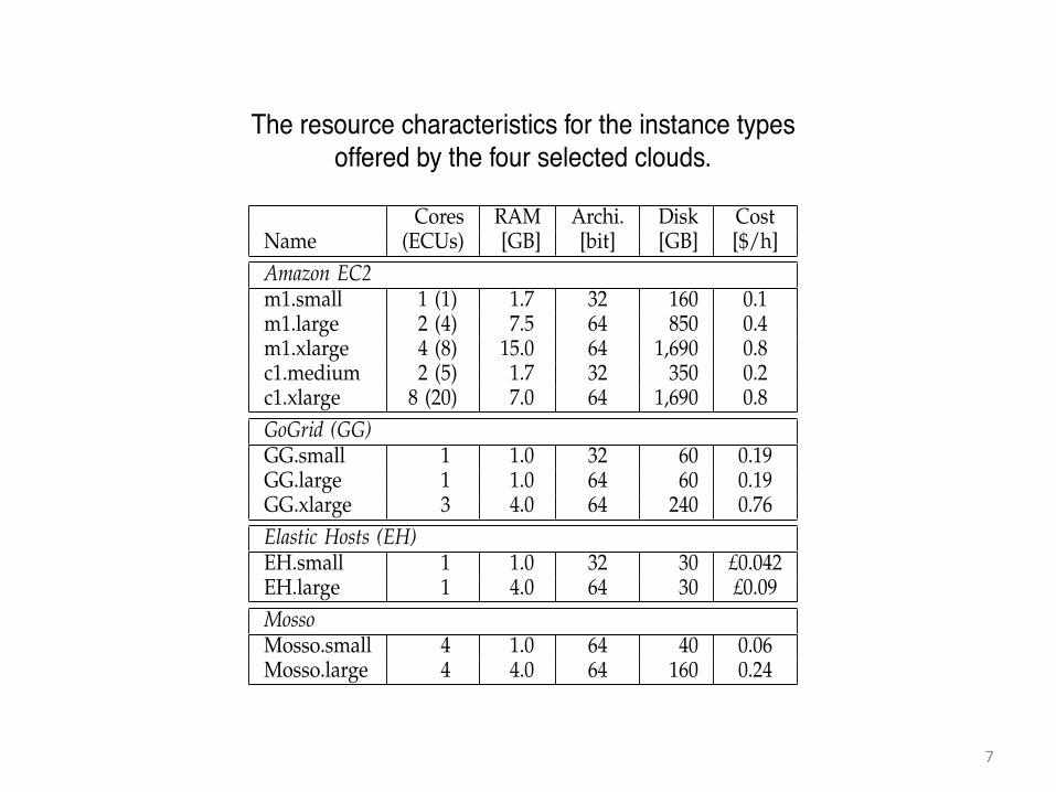
The Amazon Elastic Computing Cloud (EC2) is anIaaS cloud computing service that opens Amazon’s largecomputing infrastructure to its users. The service iselastic in the sense that it enables the user to extendor shrink its infrastructure by launching or terminat-ing new virtual machines (instances). The user can useany of the instance types currently available on offer,the characteristics and cost of the five instance typesavailable in June 2009 are summarized in Table 1. AnECU is the equivalent CPU power of a 1.0-1.2 GHz2007 Opteron or Xeon processor. The theoretical peakperformance can be computed for different instancesfrom the ECU definition: a 1.1 GHz 2007 Opteron canperform 4 flops per cycle at full pipeline, which meansat peak performance one ECU equals 4.4 gigaflops persecond (GFLOPS).

To create an infrastructure from EC2 resources, theuser specifies the instance type and the VM image; theuser can specify any VM image previously registeredwith Amazon, including Amazon’s or the user’s own.Once the VM image has been transparently deployedon a physical machine (the resource status is running),the instance is booted; at the end of the boot process theresource status becomes installed. The installed resourcecan be used as a regular computing node immedi-ately after the booting process has finished, via an sshconnection. A maximum of 20 instances can be usedconcurrently by regular users by default; an application

can be made to increase this limit, but the processinvolves an Amazon representative. Amazon EC2 abidesby a Service Level Agreement (SLA) in which the useris compensated if the resources are not available foracquisition at least 99.95% of the time. The security of theAmazon services has been investigated elsewhere [10].

3 MTC PRESENCE IN SCIENTIFIC COMPUT-ING WORKLOADSAn important assumption of this work is that the existingscientific workloads already include Many Task Comput-ing users, that is, of users that employ loosely coupledapplications comprising many tasks to achieve theirscientific goals. In this section we verify this assumptionthrough a detailed investigation of workload traces takenfrom real scientific computing environments.

3.1 Method and Experimental SetupMTC workloads may comprise tens of thousands tohundreds of thousands of tasks and BoTs [4], and atypical period may be one year or the whole trace. Ourmethod for identifying proto-MTC users—users witha pronounced MTC-like workload, which are potentialMTC users in the future—in existing system workloadsis based on the identification of users with many sub-mitted tasks and/or bags-of-tasks in the workload tracestaken from real scientific computing infrastructures. Wedefine an MTC user to be a user that has submitted atleast J jobs and at least B bags-of-tasks. The user part ofour definition serves as a coupling between jobs, underthe assumption that a user submits jobs for executiontowards an arbitrary but meaningful goal. The jobs partensures that we focus on high-volume users; these usersare likely to need new scheduling techniques for goodsystem performance. The bag-of-tasks part ensures thattask submission occurs within a short period of time; thissubmission pattern raises new challenges in the area oftask scheduling and management [4]. Ideally, it shouldbe possible to use a unique pair of values for J and Bacross different systems.

To investigate the presence of an MTC component inexisting scientific computing infrastructures we analyzeten workload traces. Table 2 summarizes the character-istics of the ten traces; see [13], [16] for more detailsabout each trace. The ID of the trace indicates the systemfrom which it was taken. The traces have been collectedfrom a wide variety of grids and parallel productionenvironments. The traces precede the existence of MTCtools; thus, the presence of an MTC component in thesetraces indicates the existence of proto-MTC users, whowill be likely to use today’s MTC-friendly environments.

To identify MTC users, we first formulate the identi-fication criterion by selecting values for J , B. If B ! 1,we first identify the BoTs in the trace using the methodthat we introduced in our previous work [22], that is,we use the BoT identification information when it is

7

MTC Presence in Scientific Computing Workloads

•  What is Many-‐Task Compu+ng ? •  Identification of users with many submitted

tasks and/or bags-of-tasks in workload traces taken from real scientific computing infrastructures.

•  Definition: MTC user is a user that has submitted at least J jobs and at least B bags-of-tasks.

8

•  Ten different workloads were analyzed to investigate the presence of MTC component:


TABLE 2The characteristics of the workload traces.

Trace ID, Trace SystemSource (Trace ID Time Number of Size Loadin Archive) [mo.] Jobs Users Sites CPUs [%]

Grid Workloads Archive [13], 6 traces1. DAS-2 (1) 18 1.1M 333 5 0.4K 15+2. RAL (6) 12 0.2M 208 1 0.8K 85+3. GLOW (7) 3 0.2M 18 1 1.6K 60+4. Grid3 (8) 18 1.3M 19 29 3.5K -5. SharcNet (10) 13 1.1M 412 10 6.8K -6. LCG (11) 1 0.2M 216 200+ 24.4K -

Parallel Workloads Archive [16], 4 traces7. CTC SP2 (6) 11 0.1M 679 1 0.4K 668. SDSC SP2 (9) 24 0.1M 437 1 0.1K 839. LANLO2K (10) 5 0.1M 337 1 2.0K 6410. SDSC DS (19) 13 0.1M 460 1 1.7K 63

present in the trace, and identify BoTs as groups of taskssubmitted by the same user at and during short timeintervals, otherwise. (We have investigated the effectof the time frame in the identification of BoTs in ourprevious work [22].) Then, we eliminate the users thathave not submitted at least B BoTs. Last, from theremaining users we select the users that have submittedat least J tasks.

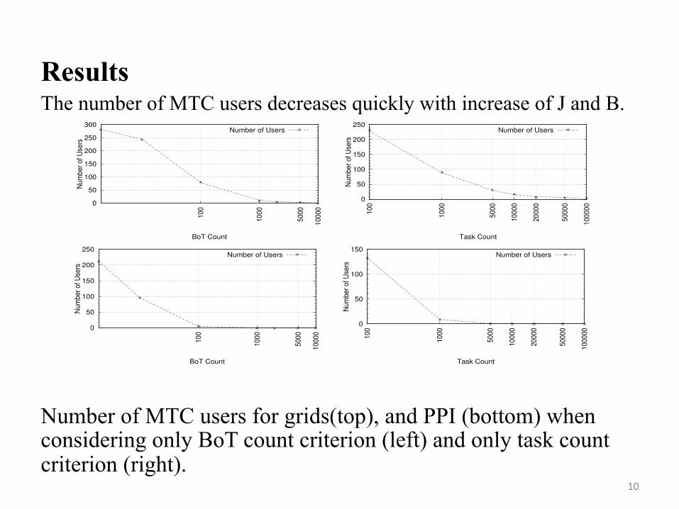
3.2 ResultsThe number of MTC users decreases quickly withthe increase of J and B. Figure 1 shows the resultsfor our analysis where we use the number of submittedBoTs (left), and the number of submitted tasks (right) ascriteria for identifying MTC users for the DAS-2 (top)and SDSC SP2 (bottom) traces. As expected, the numberof MTC users identified in the workload traces decreasesas the number of submitted BoTs/tasks increases. Thenumber of MTC users identified in the trace decreasesmuch faster in the SDSC trace than in the DAS-2 tracewith the increase of the number of BoTs/tasks. In ad-dition, since there are not many MTC users for largenumber of BoTs/tasks in PPI, we see evidence that thereis more MTC activity in grids than in PPI.

Expectedly, there is more MTC-like activity in gridsthan in PPIs. To compare the MTC-like activity of gridsand PPIs we analyze for each trace the percentage ofMTC jobs from the total number of jobs, and the percent-age of CPU time consumed by MTC jobs from the totalCPU time consumption recorded in the trace. Table 3presents the results for various simple and complexcriteria for all traces. We use ”number of BoTs submitted! 100” and ”number of jobs submitted ! 1,000” as thesimple criteria, and ”number of BoTs submitted ! 1,000& number of tasks submitted ! 10,000” as the complexcriterion. Even for the simple criteria, we observe thatfor PPIs, except for the LANL-O2K trace, there are noMTC jobs for large values of B (the number of BoTs). Asthe number of BoTs and tasks increases, the percentageof MTC jobs and their consumed CPU-time decrease forboth PPI and grids, as expected. However, for the Grid3

and GLOW traces the MTC activity is highly presenteven for large values of J and B.It turns out that thecomplex criterion additionally selects mostly users whosubmit many single-node tasks (not shown). Since thistype of proto-MTC workload has the potential to executewell in any environment, including clouds, we select anduse this complex criterion for the remainder of this work.

4 CLOUD PERFORMANCE EVALUATIONIn this section we present an empirical performanceevaluation of cloud computing services. Toward thisend, we run micro-benchmarks and application kernelstypical for scientific computing on cloud computingresources, and compare whenever possible the obtainedresults to the theoretical peak performance and/or theperformance of other scientific computing systems.

4.1 MethodOur method stems from the traditional system bench-marking. Saavedra and Smith [23] have shown thatbenchmarking the performance of various system com-ponents with a wide variety of micro-benchmarks andapplication kernels can provide a first order estimateof that system’s performance. Similarly, in this sectionwe evaluate various components of the four cloudsintroduced in Section 2.2. However, our method is nota straightforward application of Saavedra and Smith’smethod. Instead, we add a cloud-specific component,select several benchmarks for a comprehensive platform-independent evaluation, and focus on metrics specific tolarge-scale systems (such as efficiency and variability).

Cloud-specific evaluation An attractive promise ofclouds is that they can always provide resources ondemand, without additional waiting time [20]. How-ever, since the load of other large-scale systems variesover time due to submission patterns [5], [6] we wantto investigate if large clouds can indeed bypass this

TABLE 3The percentage of MTC jobs, and the CPU time

consumed by these jobs from the total number of jobsand consumed CPU time for all traces, with varioussimple and complex criteria for identifying MTC users.

CPUT stands for Total CPU Time.

Simple criteria Complex criterionJobs ! 10,000 &

BoTs ! 100 Tasks ! 1,000 BoTs ! 1,000Jobs CPUT Jobs CPUT Jobs CPUT

Trace ID [%] [%] [%] [%] [%] [%]DAS-2 90 65 95 73 57 26RAL 81 78 98 94 33 28GLOW 95 75 99 91 83 69Grid3 100 97 100 97 97 95SharcNet 40 35 95 85 15 9LCG 61 39 87 61 0 0CTC SP2 16 13 18 14 0 0SDSC SP2 13 93 25 6 0 0LANL O2 66 14 73 18 34 6SDSC DS 29 7 44 18 0 0

9

Results The number of MTC users decreases quickly with increase of J and B.

Number of MTC users for grids(top), and PPI (bottom) when considering only BoT count criterion (left) and only task count criterion (right).


0

50

100

150

200

250

300

100

100

0

500

0

100

00

Num

ber

of U

sers

BoT Count

Number of Users

0

50

100

150

200

250

100

100

0

500

0

100

00

200

00

500

00

100

000

Num

ber

of U

sers

Task Count

Number of Users

0

50

100

150

200

250

100

100

0

500

0

100

00

Num

ber

of U

sers

BoT Count

Number of Users

0

50

100

150

100

100

0

500

0

100

00

200

00

500

00

100

000

Num

ber

of U

sers

Task Count

Number of Users

Fig. 1. Number of MTC users for the DAS-2 trace (top), and the San Diego Supercomputer Center (SDSC) SP2 trace(bottom) when considering only the submitted BoT count criterion (left), and only submitted task count criterion (right).

TABLE 4The benchmarks used for cloud performance evaluation.

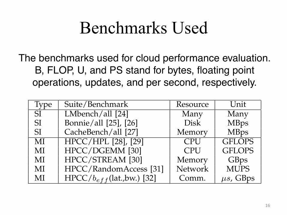
B, FLOP, U, and PS stand for bytes, floating pointoperations, updates, and per second, respectively.

Type Suite/Benchmark Resource UnitSI LMbench/all [24] Many ManySI Bonnie/all [25], [26] Disk MBpsSI CacheBench/all [27] Memory MBpsMI HPCC/HPL [28], [29] CPU GFLOPSMI HPCC/DGEMM [30] CPU GFLOPSMI HPCC/STREAM [30] Memory GBpsMI HPCC/RandomAccess [31] Network MUPSMI HPCC/beff (lat.,bw.) [32] Comm. µs, GBps

problem. To this end, one or more instances of thesame instance type are repeatedly acquired and releasedduring a few minutes; the resource acquisition requestsfollow a Poisson process with arrival rate ! = 1s!1.

Infrastructure-agnostic evaluation There currently isno single accepted benchmark for scientific computing atlarge-scale. To address this issue, we use several tradi-tional benchmark suites comprising micro-benchmarksand (scientific) application kernels. We further designtwo types of test workloads: SI–run one or more single-process jobs on a single instance (possibly with multiplecores), and MI–run a single multi-process job on multipleinstances. The SI workloads execute in turn one of theLMbench [33], Bonnie [34], and CacheBench [35] bench-mark suites. The MI workloads execute the HPC Chal-lenge Benchmark (HPCC) [28] scientific computing bench-mark suite. The characteristics of the used benchmarksand the mapping to the test workloads are summarizedin Table 4; we refer to the benchmarks’ references formore details.

Performance metrics We use the performance metricsdefined by the benchmarks presented in Table 4. We

TABLE 5The VM images used in our experiments.

VM image OS, MPI Archi BenchmarksEC2/ami-2bb65342 FC6 32bit SIEC2/ami-36ff1a5f FC6 64bit SIEC2/ami-3e836657 FC6, MPI 32bit MIEC2/ami-e813f681 FC6, MPI 64bit MIGG/server1 RHEL 5.1, MPI 32&64bit SI&MIEH/server1 Knoppix 5.3.1 32bit SIEH/server2 Ubuntu 8.10 64bit SIMosso/server1 Ubuntu 8.10 32&64bit SI

also define and use the HPL efficiency of a virtual clusterbased on the instance type T as the ratio between theHPL benchmark performance of the real cluster and thepeak theoretical performance of a same-sized T-cluster,expressed as a percentage. Job execution at large-scaleoften leads to performance variability. To address thisproblem, in this work we report not only the averageperformance, but also the variability of the results.

4.2 Experimental SetupWe now describe the experimental setup in which we usethe performance evaluation method presented earlier.

Performance Analysis Tool We have recently [36]extended the GrenchMark [37] large-scale distributedtesting framework with new features which allow itto test cloud computing infrastructures. The frameworkwas already able to generate and submit both real andsynthetic workloads to grids, clusters, clouds, and otherlarge-scale distributed environments. For this work, wehave added to GrenchMark the ability to execute andanalyze the benchmarks described in the previous sec-tion.

Environment We perform our measurements on ho-mogeneous virtual environments built from virtual re-

10

•  There is more MTC like activity in grids than in PPIs. •  To compare the MTC-like activity of grids and PPIs we

analyze for each trace the percentage of MTC jobs from the total number of jobs, and the percentage of CPU time consumed by MTC jobs from the total CPU time consumption recorded in the trace.

•  The following table presents the results for various simple and complex criteria for all traces


TABLE 2The characteristics of the workload traces.

Trace ID, Trace SystemSource (Trace ID Time Number of Size Loadin Archive) [mo.] Jobs Users Sites CPUs [%]

Grid Workloads Archive [13], 6 traces1. DAS-2 (1) 18 1.1M 333 5 0.4K 15+2. RAL (6) 12 0.2M 208 1 0.8K 85+3. GLOW (7) 3 0.2M 18 1 1.6K 60+4. Grid3 (8) 18 1.3M 19 29 3.5K -5. SharcNet (10) 13 1.1M 412 10 6.8K -6. LCG (11) 1 0.2M 216 200+ 24.4K -

Parallel Workloads Archive [16], 4 traces7. CTC SP2 (6) 11 0.1M 679 1 0.4K 668. SDSC SP2 (9) 24 0.1M 437 1 0.1K 839. LANLO2K (10) 5 0.1M 337 1 2.0K 6410. SDSC DS (19) 13 0.1M 460 1 1.7K 63

present in the trace, and identify BoTs as groups of taskssubmitted by the same user at and during short timeintervals, otherwise. (We have investigated the effectof the time frame in the identification of BoTs in ourprevious work [22].) Then, we eliminate the users thathave not submitted at least B BoTs. Last, from theremaining users we select the users that have submittedat least J tasks.

3.2 ResultsThe number of MTC users decreases quickly withthe increase of J and B. Figure 1 shows the resultsfor our analysis where we use the number of submittedBoTs (left), and the number of submitted tasks (right) ascriteria for identifying MTC users for the DAS-2 (top)and SDSC SP2 (bottom) traces. As expected, the numberof MTC users identified in the workload traces decreasesas the number of submitted BoTs/tasks increases. Thenumber of MTC users identified in the trace decreasesmuch faster in the SDSC trace than in the DAS-2 tracewith the increase of the number of BoTs/tasks. In ad-dition, since there are not many MTC users for largenumber of BoTs/tasks in PPI, we see evidence that thereis more MTC activity in grids than in PPI.

Expectedly, there is more MTC-like activity in gridsthan in PPIs. To compare the MTC-like activity of gridsand PPIs we analyze for each trace the percentage ofMTC jobs from the total number of jobs, and the percent-age of CPU time consumed by MTC jobs from the totalCPU time consumption recorded in the trace. Table 3presents the results for various simple and complexcriteria for all traces. We use ”number of BoTs submitted! 100” and ”number of jobs submitted ! 1,000” as thesimple criteria, and ”number of BoTs submitted ! 1,000& number of tasks submitted ! 10,000” as the complexcriterion. Even for the simple criteria, we observe thatfor PPIs, except for the LANL-O2K trace, there are noMTC jobs for large values of B (the number of BoTs). Asthe number of BoTs and tasks increases, the percentageof MTC jobs and their consumed CPU-time decrease forboth PPI and grids, as expected. However, for the Grid3

and GLOW traces the MTC activity is highly presenteven for large values of J and B.It turns out that thecomplex criterion additionally selects mostly users whosubmit many single-node tasks (not shown). Since thistype of proto-MTC workload has the potential to executewell in any environment, including clouds, we select anduse this complex criterion for the remainder of this work.

4 CLOUD PERFORMANCE EVALUATIONIn this section we present an empirical performanceevaluation of cloud computing services. Toward thisend, we run micro-benchmarks and application kernelstypical for scientific computing on cloud computingresources, and compare whenever possible the obtainedresults to the theoretical peak performance and/or theperformance of other scientific computing systems.

4.1 MethodOur method stems from the traditional system bench-marking. Saavedra and Smith [23] have shown thatbenchmarking the performance of various system com-ponents with a wide variety of micro-benchmarks andapplication kernels can provide a first order estimateof that system’s performance. Similarly, in this sectionwe evaluate various components of the four cloudsintroduced in Section 2.2. However, our method is nota straightforward application of Saavedra and Smith’smethod. Instead, we add a cloud-specific component,select several benchmarks for a comprehensive platform-independent evaluation, and focus on metrics specific tolarge-scale systems (such as efficiency and variability).

Cloud-specific evaluation An attractive promise ofclouds is that they can always provide resources ondemand, without additional waiting time [20]. How-ever, since the load of other large-scale systems variesover time due to submission patterns [5], [6] we wantto investigate if large clouds can indeed bypass this

TABLE 3The percentage of MTC jobs, and the CPU time

consumed by these jobs from the total number of jobsand consumed CPU time for all traces, with varioussimple and complex criteria for identifying MTC users.

CPUT stands for Total CPU Time.

Simple criteria Complex criterionJobs ! 10,000 &

BoTs ! 100 Tasks ! 1,000 BoTs ! 1,000Jobs CPUT Jobs CPUT Jobs CPUT

Trace ID [%] [%] [%] [%] [%] [%]DAS-2 90 65 95 73 57 26RAL 81 78 98 94 33 28GLOW 95 75 99 91 83 69Grid3 100 97 100 97 97 95SharcNet 40 35 95 85 15 9LCG 61 39 87 61 0 0CTC SP2 16 13 18 14 0 0SDSC SP2 13 93 25 6 0 0LANL O2 66 14 73 18 34 6SDSC DS 29 7 44 18 0 0

11

•  For PPIs, except for the LANL-O2K trace, there are no MTC jobs for large values of B.

•  As the values of B, J and number of tasks increase, the percentage of MTC jobs and their consumed CPU-time decreases for both PPI and grids.

12

Cloud Performance Evaluation

Method Benchmarking the performance of various systems components with a wide variety of benchmarks can provide a good estimate of system’s performance. Cloud-specific evaluation: one or more instances of the same instance type are repeatedly acquired and released over a short period of time and the delay is observed. Infrastructure-agnostic evaluation: Two types of test workloads are designed S1: run one or more single process jobs on a single instance. M1: run a single multi-process job on multiple instances.

13

Benchmarks used

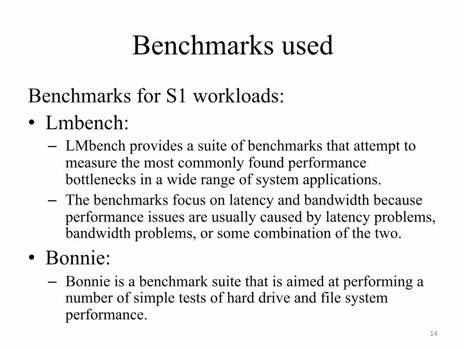
Benchmarks for S1 workloads: •  Lmbench: –  LMbench provides a suite of benchmarks that attempt to

measure the most commonly found performance bottlenecks in a wide range of system applications.

–  The benchmarks focus on latency and bandwidth because performance issues are usually caused by latency problems, bandwidth problems, or some combination of the two.

•  Bonnie: –  Bonnie is a benchmark suite that is aimed at performing a

number of simple tests of hard drive and file system performance.

14

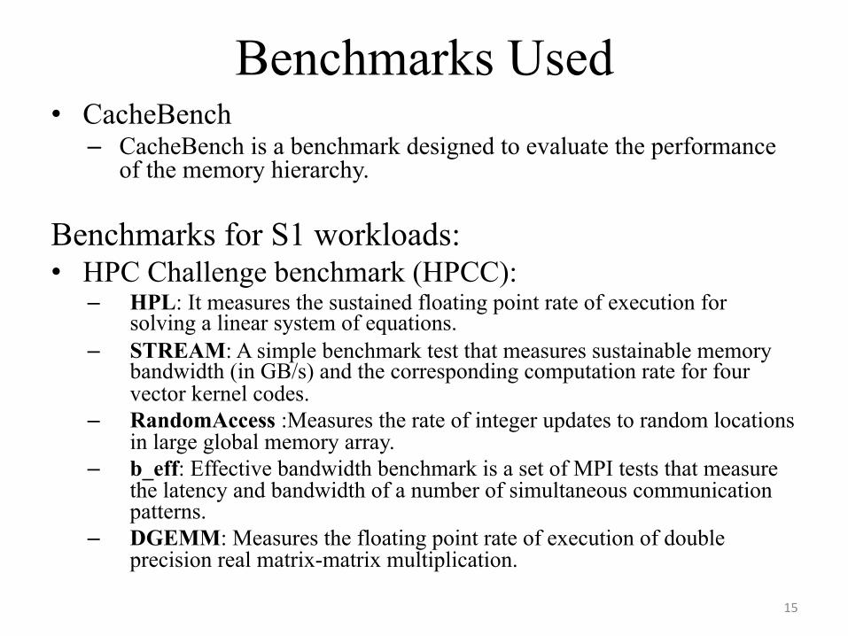
Benchmarks Used •  CacheBench –  CacheBench is a benchmark designed to evaluate the performance

of the memory hierarchy.

Benchmarks for S1 workloads: •  HPC Challenge benchmark (HPCC):

–  HPL: It measures the sustained floating point rate of execution for solving a linear system of equations.

–  STREAM: A simple benchmark test that measures sustainable memory bandwidth (in GB/s) and the corresponding computation rate for four vector kernel codes.

–  RandomAccess :Measures the rate of integer updates to random locations in large global memory array.

–  b_eff: Effective bandwidth benchmark is a set of MPI tests that measure the latency and bandwidth of a number of simultaneous communication patterns.

–  DGEMM: Measures the floating point rate of execution of double precision real matrix-matrix multiplication.

15

Benchmarks Used


0

50

100

150

200

250

300

100

1000

5000

10000

Num

ber

of U

sers

BoT Count

Number of Users

0

50

100

150

200

250

100

1000

5000

10000

20000

50000

100000

Num

ber

of U

sers

Task Count

Number of Users

0

50

100

150

200

250

100

1000

5000

10000

Num

ber

of U

sers

BoT Count

Number of Users

0

50

100

150

100

1000

5000

10000

20000

50000

100000

Num

ber

of U

sers

Task Count

Number of Users














16

Experimental Setup

•  Performance Analysis Tool: –  The GrenchMark tool has been extended to execute and

analyze the benchmarks. –  Used for •  Generation of synthetic workloads •  Performance testing and analysis •  Jobs throughput comparison of two grid systems

17

Experimental Setup

•  Environment: •  The VM images used are summarized in the following table:


0

50

100

150

200

250

300

10

0

10

00

50

00

10

00

0

Nu

mb

er

of

Use

rs

BoT Count

Number of Users

0

50

100

150

200

250

10

0

10

00

50

00

10

00

0

20

00

0

50

00

0

10

00

00

Nu

mb

er

of

Use

rs

Task Count

Number of Users

0

50

100

150

200

250 1

00

10

00

50

00

10

00

0

Nu

mb

er

of

Use

rs

BoT Count

Number of Users

0

50

100

150

10

0

10

00

50

00

10

00

0

20

00

0

50

00

0

10

00

00

Nu

mb

er

of

Use

rs

Task Count

Number of Users














18

Experimental Setup •  Message Passing Interface (MPI) Library and

network: –  For MI (parallel) experiments, the network selection can be

critical for achieving good results. –  Amazon EC2 and GoGrid use internal IP addresses (within a

cloud). –  Traffic between internal IPs is free, while the traffic to and from

the Internet IPs is not.

•  Optimization, tuning: –  The benchmarks were compiled using GNU C/C++

4.1 with the –O3 –fnuroll –loops command line arguments

19

Results •  Resource Acquisi+on and Release:

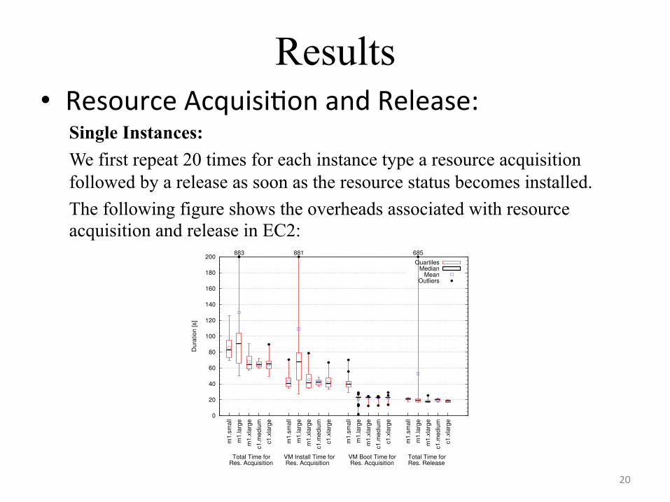
Single Instances: We first repeat 20 times for each instance type a resource acquisition followed by a release as soon as the resource status becomes installed. The following figure shows the overheads associated with resource acquisition and release in EC2:


0

20

40

60

80

100

120

140

160

180

200

m1

.sm

all

m1

.larg

e

m1

.xla

rge

c1.m

ed

ium

c1.x

larg

e

m1

.sm

all

m1

.larg

e

m1

.xla

rge

c1.m

ed

ium

c1.x

larg

e

m1

.sm

all

m1

.larg

e

m1

.xla

rge

c1.m

ed

ium

c1.x

larg

e

m1

.sm

all

m1

.larg

e

m1

.xla

rge

c1.m

ed

ium

c1.x

larg

e

Du

ratio

n [

s]

Total Time forRes. Acquisition

VM Boot Time for Res. Acquisition

VM Install Time for Res. Acquisition

Total Time forRes. Release

883 881 685

QuartilesMedian

MeanOutliers

Fig. 2. Resource acquisition and release overheadsfor acquiring single EC2 instances.

0

20

40

60

80

100

120

2 4 8 16 20 2 4 8 16 20 2 4 8 16 20 2 4 8 16 20

Du

ratio

n [

s]

Instance Count Instance Count Instance Count Instance Count Total Time forRes. Acquisition




QuartilesMedian

MeanOutliers

Fig. 3. Single-instance resource acquisitionand release overheads when acquiring multiplec1.xlarge instances at the same time.

0

2

4

6

8

10

m1.small m1.large m1.xlarge c1.medium c1.xlarge

Perf

orm

ance

[G

OP

S]

Instance Type

INT-bit INT-add INT-mul INT64-bit INT64-mul

0

0.2

0.4

0.6

0.8

1


Perf

orm

ance

[G

OP

S]

Instance Type

FLOAT-addFLOAT-mul

FLOAT-bogoDOUBLE-add

DOUBLE-mulDOUBLE-bogo

0

2

4

6

8

10

EH.small EH.large GG.small GG.large GG.xlarge Mosso.small Mosso.large

Perf

orm

ance

[G

OP

S]

Instance Type


0

0.2

0.4

0.6

0.8

1


Perf

orm

ance

[G

OP

S]

Instance Type

FLOAT-addFLOAT-mul



Fig. 4. LMbench results (top) for the EC2 instances, and (bottom) for the other instances. Each row depictsthe performance of 32- and 64-bit integer operations in giga-operations per second (GOPS) (left), and of floatingoperations with single and double precision (right).

maximum of ECU (4.4 GOPS). A potential reason for thissituation is the over-run or thrashing of the memorycaches by the working sets of other applications sharingthe same physical machines; a study independent fromours [44] identifies the working set size as a key parame-ter to consider when placing and migrating applicationson virtualized servers. This situation occurs especiallywhen the physical machines are shared among usersthat are unaware of each other; a previous study [45]has found that even instances of the same user may belocated on the same physical machine. The performanceevaluation results also indicate that the double-precisionfloat performance of the c1.* instances, arguably themost important for scientific computing, is mixed: excel-lent addition but poor multiplication capabilities. Thus,

as many scientific computing applications use heavilyboth of these operations, the user is faced with the diffi-cult problem of selecting between two wrong choices. Fi-nally, several double and float operations take longer onc1.medium than on m1.small. For the other instances,EH.* and Mosso.* instances have similar performancefor both integer and floating point operations. GG.*instances have the best float and double-precision per-formance, and good performance for integer operations,which suggests the existence of better hardware supportfor these operations on these instances.

I/O performance We assess in two steps the I/Operformance of each instance type with the Bonniebenchmarking suite. The first step is to determine thesmallest file size that invalidates the memory-based I/O

20

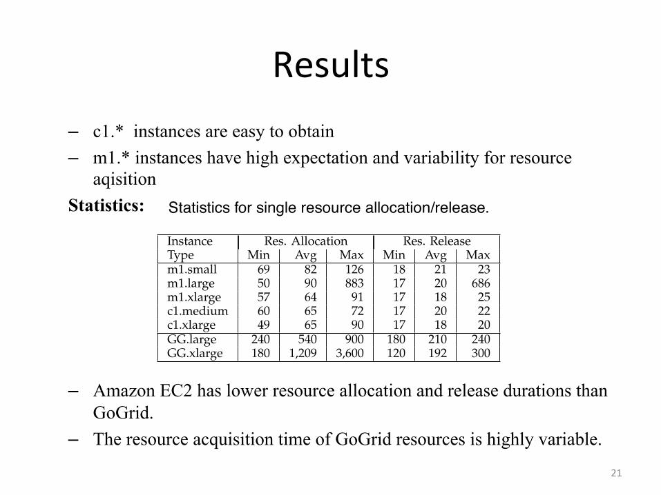
Results –  c1.* instances are easy to obtain –  m1.* instances have high expectation and variability for resource

aqisition Statistics:

–  Amazon EC2 has lower resource allocation and release durations than GoGrid.

–  The resource acquisition time of GoGrid resources is highly variable.


sources belonging to one of the instance types describedin Table 1; the used VM images are summarized inTable 5. The experimental environments comprise from1 to 128 cores. Except for the use of internal IP addresses,described below, we have used in all our experiments thestandard configurations provided by the cloud. Due toour choice of benchmarks, our Single-Job results can bereadily compared with the benchmarking results madepublic for many other scientific computing systems, andin particular by the HPCC effort [38].

MPI library and network The VM images used for theHPCC benchmarks also have a working pre-configuredMPI based on the mpich2-1.0.5 [39] implementation.For the MI (parallel) experiments, the network selec-tion can be critical for achieving good results. AmazonEC2 and GoGrid, the two clouds for which we haveperformed MI experiments, use internal IP addresses(IPs), that is, the IPs accessible only within the cloud,to optimize the data transfers between closely-locatedinstances. (This also allows the clouds to better shape thetraffic and to reduce the number of Internet-accessibleIPs, and in turn to reduce the cloud’s operational costs.)EC2 and GoGrid give strong incentives to their cus-tomers to use internal IP addresses, in that the networktraffic between internal IPs is free, while the traffic toor from the Internet IPs is not. We have used onlythe internal IP addresses in our experiments with MIworkloads.

Optimizations, tuning The benchmarks were com-piled using GNU C/C++ 4.1 with the-O3 -funroll-loops command-line arguments. Wedid not use any additional architecture- or instance-dependent optimizations. For the HPL benchmark, theperformance results depend on two main factors: the theBasic Linear Algebra Subprogram (BLAS) [40] library,and the problem size. We used in our experiments theGotoBLAS [41]library, which is one of the best portablesolutions freely available to scientists. Searching for theproblem size that can deliver peak performance is anextensive (and costly) process. Instead, we used a freeanalytical tool [42] to find for each system the problemsizes that can deliver results close to the peak perfor-mance; based on the tool advice we have used valuesfrom 13,000 to 110,000 for N, the size (order) of thecoefficient matrix A [28], [43].

4.3 ResultsThe experimental results of the Amazon EC2 perfor-mance evaluation are presented in the following.

4.3.1 Resource Acquisition and ReleaseWe study two resource acquisition and release scenarios:for single instances, and for multiple instances allocatedat once.

Single instances We first repeat 20 times for eachinstance type a resource acquisition followed by a releaseas soon as the resource status becomes installed (see

TABLE 6Statistics for single resource allocation/release.

Instance Res. Allocation Res. ReleaseType Min Avg Max Min Avg Maxm1.small 69 82 126 18 21 23m1.large 50 90 883 17 20 686m1.xlarge 57 64 91 17 18 25c1.medium 60 65 72 17 20 22c1.xlarge 49 65 90 17 18 20GG.large 240 540 900 180 210 240GG.xlarge 180 1,209 3,600 120 192 300

Section 2.2). Figure 2 shows the overheads associatedwith resource acquisition and release in EC2. The totalresource acquisition time (Total) is the sum of the Installand Boot times. The Release time is the time taken torelease the resource back to EC2; after it is releasedthe resource stops being charged by Amazon. The c1.*instances are surprisingly easy to obtain; in contrast, them1.* instances have for the resource acquisition timehigher expectation (63-90s compared to around 63s) andvariability (much larger boxes). With the exception ofthe occasional outlier, both the VM Boot and Releasetimes are stable and represent about a quarter of Totaleach. Table 6 presents basic statistics for single resourceallocation and release. Overall, Amazon EC2 has oneorder of magnitude lower single resource allocationand release durations than GoGrid. From the EC2resources, the m1.small and m1.large instances havehigher average allocation duration, and exhibit outlierscomparable to those encountered for GoGrid. The re-source acquisition time of GoGrid resources is highlyvariable; here, GoGrid behaves similarly to to grids [5]and unlike the promise of clouds.

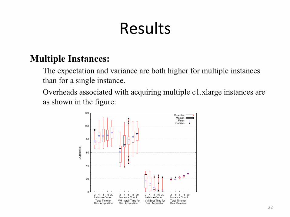
Multiple instances We investigate next the perfor-mance of requesting the acquisition of multiple resources(2,4,8,16, and 20) at the same time; a scenario common forcreating homogeneous virtual clusters. When resourcesare requested in bulk, we record acquisition and releasetimes for each resource in the request, separately. Fig-ure 3 shows the basic statistical properties of the timesrecorded for c1.xlarge instances. The expectation andthe variance are both higher for multiple instances thanfor a single instance.

4.3.2 Single-Machine BenchmarksIn this set of experiments we measure the raw perfor-mance of the CPU, I/O, and memory hierarchy usingthe Single-Instance benchmarks listed in Section 4.1. Werun each benchmark 10 times and report the averageresults.

Compute performance We assess the computationalperformance of each instance type using the entire LM-bench suite. The performance of int and int64 operations,and of the float and double-precision float operationsis depicted in Figure 4 left and right, respectively. TheGOPS recorded for the floating point and double-precisionfloat operations is six to eight times lower than the theoretical

21

Results Multiple Instances:

The expectation and variance are both higher for multiple instances than for a single instance. Overheads associated with acquiring multiple c1.xlarge instances are as shown in the figure:


0

20

40

60

80

100

120

140

160

180

200

m1.s

mall

m1.la

rge

m1.x

larg

e

c1.m

ediu

m

c1.x

larg

e

m1.s

mall

m1.la

rge

m1.x

larg

e

c1.m

ediu

m

c1.x

larg

e

m1.s

mall

m1.la

rge

m1.x

larg

e

c1.m

ediu

m

c1.x

larg

e

m1.s

mall

m1.la

rge

m1.x

larg

e

c1.m

ediu

m

c1.x

larg

e

Dura

tion [s]





883 881 685

QuartilesMedian

MeanOutliers


0

20

40

60

80

100

120

2 4 8 16 20 2 4 8 16 20 2 4 8 16 20 2 4 8 16 20

Dura

tion [s]





QuartilesMedian

MeanOutliers


0

2

4

6

8

10


Perf

orm

ance

[G

OP

S]

Instance Type


0

0.2

0.4

0.6

0.8

1


Perf

orm

ance

[G

OP

S]

Instance Type

FLOAT-addFLOAT-mul



0

2

4

6

8

10


Perf

orm

ance

[G

OP

S]

Instance Type


0

0.2

0.4

0.6

0.8

1


Perf

orm

ance

[G

OP

S]

Instance Type

FLOAT-addFLOAT-mul







22

Results •  Single-Machine Benchmarks

Compute performance: Computational performance is accessed using the entire Lmbench suite. LMbench results (top) for the EC2 instances, and (bottom) for the other instances. Each row depicts the performance of 32- and 64-bit integer operations in giga-operations per second (GOPS) (left), and of floating operations with single and double precision (right).


0

20

40

60

80

100

120

140

160

180

200

m1

.sm

all

m1

.larg

e

m1

.xla

rge

c1.m

ed

ium

c1.x

larg

e

m1

.sm

all

m1

.larg

e

m1

.xla

rge

c1.m

ed

ium

c1.x

larg

e

m1

.sm

all

m1

.larg

e

m1

.xla

rge

c1.m

ed

ium

c1.x

larg

e

m1

.sm

all

m1

.larg

e

m1

.xla

rge

c1.m

ed

ium

c1.x

larg

e

Du

ratio

n [

s]





883 881 685

QuartilesMedian

MeanOutliers


0

20

40

60

80

100

120

2 4 8 16 20 2 4 8 16 20 2 4 8 16 20 2 4 8 16 20

Du

ratio

n [

s]





QuartilesMedian

MeanOutliers


0

2

4

6

8

10


Perf

orm

ance

[G

OP

S]

Instance Type


0

0.2

0.4

0.6

0.8

1


Perf

orm

ance

[G

OP

S]

Instance Type

FLOAT-addFLOAT-mul



0

2

4

6

8

10


Perf

orm

ance

[G

OP

S]

Instance Type


0

0.2

0.4

0.6

0.8

1


Perf

orm

ance

[G

OP

S]

Instance Type

FLOAT-addFLOAT-mul







23

Results –  The GOPS recorded for the floating point and double-precision float

operations is six to eight times lower than the theoretical maximum of ECU (4.4 GOPS).

–  The double-precision float performance of the c1.* instances, arguably the most important for scientific computing, is mixed: excel- lent addition but poor multiplication capabilities.

I/O Performance: It is accessed in two steps: –  The first step is to determine the smallest file size that invalidates the

memory-based I/O cache, by running the Bonnie suite for thirteen file sizes in the range 1024 Kilo-binary byte (KiB) to 40 GiB.

–  The results obtained for the file sizes above 5GiB correspond to the real I/O performance of the system; lower file sizes would be served by the system with a combination of memory and disk operations.

24

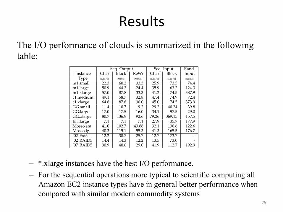
Results The I/O performance of clouds is summarized in the following table:

–  *.xlarge instances have the best I/O performance. –  For the sequential operations more typical to scientific computing all

Amazon EC2 instance types have in general better performance when compared with similar modern commodity systems


TABLE 7The I/O of clouds vs. 2002 [25] and 2007 [26] systems.

Seq. Output Seq. Input Rand.Instance Char Block ReWr Char Block Input

Type [MB/s] [MB/s] [MB/s] [MB/s] [MB/s] [Seek/s]

m1.small 22.3 60.2 33.3 25.9 73.5 74.4m1.large 50.9 64.3 24.4 35.9 63.2 124.3m1.xlarge 57.0 87.8 33.3 41.2 74.5 387.9c1.medium 49.1 58.7 32.8 47.4 74.9 72.4c1.xlarge 64.8 87.8 30.0 45.0 74.5 373.9GG.small 11.4 10.7 9.2 29.2 40.24 39.8GG.large 17.0 17.5 16.0 34.1 97.5 29.0GG.xlarge 80.7 136.9 92.6 79.26 369.15 157.5EH.large 7.1 7.1 7.1 27.9 35.7 177.9Mosso.sm 41.0 102.7 43.88 32.1 130.6 122.6Mosso.lg 40.3 115.1 55.3 41.3 165.5 176.7’02 Ext3 12.2 38.7 25.7 12.7 173.7 -’02 RAID5 14.4 14.3 12.2 13.5 73.0 -’07 RAID5 30.9 40.6 29.0 41.9 112.7 192.9

cache, by running the Bonnie suite for thirteen file sizesin the range 1024 Kilo-binary byte (KiB) to 40 GiB. Theresults of this preliminary step have been summarizedin a technical report [46, pp.11-12]; we only summarizethem here. For all instance types, a performance dropbegins with the 100MiB test file and ends at 2GiB,indicating a capacity of the memory-based disk cacheof 4-5GiB (twice 2GiB). Thus, the results obtained forthe file sizes above 5GiB correspond to the real I/Operformance of the system; lower file sizes would beserved by the system with a combination of memoryand disk operations. We analyze the I/O performanceobtained for files sizes above 5GiB in the second step;Table 7 summarizes the results. We find that the I/Operformance indicated by Amazon EC2 (see Table 1)corresponds to the achieved performance for randomI/O operations (column ’Rand. Input’ in Table 7). The

*.xlarge instance types have the best I/O performancefrom all instance types. For the sequential operations moretypical to scientific computing all Amazon EC2 instancetypes have in general better performance when compared withsimilar modern commodity systems, such as the systemsdescribed in the last three rows in Table 7; EC2 maybe using better hardware, which is affordable due toeconomies of scale [20].

4.3.3 Multi-Machine BenchmarksIn this set of experiments we measure the performancedelivered by homogeneous clusters formed with Ama-zon EC2 and GoGrid instances when running the Single-Job-Multi-Machine benchmarks. For these tests we ex-ecute 5 times the HPCC benchmark on homogeneousclusters of 1–16 (1–8) instances on EC2 (GoGrid), andpresent the average results.

HPL performance The performance achieved for theHPL benchmark on various virtual clusters based on them1.small and c1.xlarge instance types is depictedin Figure 5. For the m1.small resources one node wasable to achieve a performance of 1.96 GFLOPS, whichis 44.54% from the peak performance advertised by

TABLE 8HPL performance and cost comparison for various EC2

and GoGrid instance types.

Peak GFLOPS GFLOPSName Perf. GFLOPS /Unit /$1m1.small 4.4 2.0 2.0 19.6m1.large 17.6 7.1 1.8 17.9m1.xlarge 35.2 11.4 1.4 14.2c1.medium 22.0 3.9 0.8 19.6c1.xlarge 88.0 50.0 2.5 62.5GG.large 12.0 8.8 8.8 46.4GG.xlarge 36.0 28.1 7.0 37.0

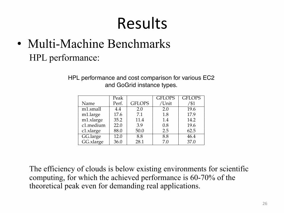
Amazon. Then, the performance increased to up to 27.8GFLOPS for 16 nodes, while the efficiency decreasedslowly to 39.4%. The results for a single c1.xlargeinstance are better: the achieved 49.97 GFLOPS represent56.78% from the advertised peak performance. However,while the performance scales when running up to 16instances to 425.82 GFLOPS, the efficiency decreases toonly 30.24%. The HPL performance loss from one to 16instances can therefore be expressed as 53.26% which re-sults in rather bad qualification for HPC applications andtheir need for fast inter-node communication. We haveobtained similar results the GG.large and GG.xlargeinstances, as shown in Figure 5. For GG.large instances,the efficiency decreases quicker than for EC2 instances,down to 47.33% while achieving 45.44 GFLOPS on eightinstances. The GG.xlarge performed even poorer in ourtests. We further investigate the performance of the HPLbenchmark for different instance types; Table 8 summa-rizes the results. The efficiency results presented in Fig-ure 5 and Table 8 place clouds below existing environmentsfor scientific computing, for which the achieved performanceis 60-70% of the theoretical peak even for demanding realapplications [47], [48], [49].

HPCC performance To obtain the performance ofvirtual EC2 and GoGrid clusters we run the HPCCbenchmarks on unit clusters comprising a single instance,and on 128-core clusters comprising 16 c1.xlarge in-stances. Table 9 summarizes the obtained results and,for comparison, results published by HPCC for fourmodern and similarly-sized HPC clusters [38]. For HPL,only the performance of the c1.xlarge is compara-ble to that of an HPC system. However, for STREAM,and RandomAccess the performance of the EC2 clustersis similar or better than the performance of the HPCclusters. We attribute this mixed behavior mainly to thenetwork characteristics: first, the EC2 platform has muchhigher latency, which has an important negative impacton the performance of the HPL benchmark; second,the network is shared among different users, a situa-tion which often leads to severe performance degrada-tion [50]. In particular, this relatively low network perfor-mance means that the ratio between the theoretical peakperformance and achieved HPL performance increaseswith the number of instances, making the virtual EC2clusters poorly scalable. Thus, for scientific computing

25

Results •  Multi-Machine Benchmarks

HPL performance: The efficiency of clouds is below existing environments for scientific computing, for which the achieved performance is 60-70% of the theoretical peak even for demanding real applications.


TABLE 7The I/O of clouds vs. 2002 [25] and 2007 [26] systems.

Seq. Output Seq. Input Rand.Instance Char Block ReWr Char Block Input

Type [MB/s] [MB/s] [MB/s] [MB/s] [MB/s] [Seek/s]

m1.small 22.3 60.2 33.3 25.9 73.5 74.4m1.large 50.9 64.3 24.4 35.9 63.2 124.3m1.xlarge 57.0 87.8 33.3 41.2 74.5 387.9c1.medium 49.1 58.7 32.8 47.4 74.9 72.4c1.xlarge 64.8 87.8 30.0 45.0 74.5 373.9GG.small 11.4 10.7 9.2 29.2 40.24 39.8GG.large 17.0 17.5 16.0 34.1 97.5 29.0GG.xlarge 80.7 136.9 92.6 79.26 369.15 157.5EH.large 7.1 7.1 7.1 27.9 35.7 177.9Mosso.sm 41.0 102.7 43.88 32.1 130.6 122.6Mosso.lg 40.3 115.1 55.3 41.3 165.5 176.7’02 Ext3 12.2 38.7 25.7 12.7 173.7 -’02 RAID5 14.4 14.3 12.2 13.5 73.0 -’07 RAID5 30.9 40.6 29.0 41.9 112.7 192.9

cache, by running the Bonnie suite for thirteen file sizesin the range 1024 Kilo-binary byte (KiB) to 40 GiB. Theresults of this preliminary step have been summarizedin a technical report [46, pp.11-12]; we only summarizethem here. For all instance types, a performance dropbegins with the 100MiB test file and ends at 2GiB,indicating a capacity of the memory-based disk cacheof 4-5GiB (twice 2GiB). Thus, the results obtained forthe file sizes above 5GiB correspond to the real I/Operformance of the system; lower file sizes would beserved by the system with a combination of memoryand disk operations. We analyze the I/O performanceobtained for files sizes above 5GiB in the second step;Table 7 summarizes the results. We find that the I/Operformance indicated by Amazon EC2 (see Table 1)corresponds to the achieved performance for randomI/O operations (column ’Rand. Input’ in Table 7). The

*.xlarge instance types have the best I/O performancefrom all instance types. For the sequential operations moretypical to scientific computing all Amazon EC2 instancetypes have in general better performance when compared withsimilar modern commodity systems, such as the systemsdescribed in the last three rows in Table 7; EC2 maybe using better hardware, which is affordable due toeconomies of scale [20].

4.3.3 Multi-Machine BenchmarksIn this set of experiments we measure the performancedelivered by homogeneous clusters formed with Ama-zon EC2 and GoGrid instances when running the Single-Job-Multi-Machine benchmarks. For these tests we ex-ecute 5 times the HPCC benchmark on homogeneousclusters of 1–16 (1–8) instances on EC2 (GoGrid), andpresent the average results.

HPL performance The performance achieved for theHPL benchmark on various virtual clusters based on them1.small and c1.xlarge instance types is depictedin Figure 5. For the m1.small resources one node wasable to achieve a performance of 1.96 GFLOPS, whichis 44.54% from the peak performance advertised by

TABLE 8HPL performance and cost comparison for various EC2

and GoGrid instance types.

Peak GFLOPS GFLOPSName Perf. GFLOPS /Unit /$1m1.small 4.4 2.0 2.0 19.6m1.large 17.6 7.1 1.8 17.9m1.xlarge 35.2 11.4 1.4 14.2c1.medium 22.0 3.9 0.8 19.6c1.xlarge 88.0 50.0 2.5 62.5GG.large 12.0 8.8 8.8 46.4GG.xlarge 36.0 28.1 7.0 37.0

Amazon. Then, the performance increased to up to 27.8GFLOPS for 16 nodes, while the efficiency decreasedslowly to 39.4%. The results for a single c1.xlargeinstance are better: the achieved 49.97 GFLOPS represent56.78% from the advertised peak performance. However,while the performance scales when running up to 16instances to 425.82 GFLOPS, the efficiency decreases toonly 30.24%. The HPL performance loss from one to 16instances can therefore be expressed as 53.26% which re-sults in rather bad qualification for HPC applications andtheir need for fast inter-node communication. We haveobtained similar results the GG.large and GG.xlargeinstances, as shown in Figure 5. For GG.large instances,the efficiency decreases quicker than for EC2 instances,down to 47.33% while achieving 45.44 GFLOPS on eightinstances. The GG.xlarge performed even poorer in ourtests. We further investigate the performance of the HPLbenchmark for different instance types; Table 8 summa-rizes the results. The efficiency results presented in Fig-ure 5 and Table 8 place clouds below existing environmentsfor scientific computing, for which the achieved performanceis 60-70% of the theoretical peak even for demanding realapplications [47], [48], [49].

HPCC performance To obtain the performance ofvirtual EC2 and GoGrid clusters we run the HPCCbenchmarks on unit clusters comprising a single instance,and on 128-core clusters comprising 16 c1.xlarge in-stances. Table 9 summarizes the obtained results and,for comparison, results published by HPCC for fourmodern and similarly-sized HPC clusters [38]. For HPL,only the performance of the c1.xlarge is compara-ble to that of an HPC system. However, for STREAM,and RandomAccess the performance of the EC2 clustersis similar or better than the performance of the HPCclusters. We attribute this mixed behavior mainly to thenetwork characteristics: first, the EC2 platform has muchhigher latency, which has an important negative impacton the performance of the HPL benchmark; second,the network is shared among different users, a situa-tion which often leads to severe performance degrada-tion [50]. In particular, this relatively low network perfor-mance means that the ratio between the theoretical peakperformance and achieved HPL performance increaseswith the number of instances, making the virtual EC2clusters poorly scalable. Thus, for scientific computing

26

Results

•  Performance Stability: Is the performance stable? The stability of different clouds has been assessed by running the LMBench and CacheBench benchmarks multiple times on the same type of virtual resources. The best-performer in terms of computation, GG.xlarge, is unstable.


0

100

200

300

400

500

1 2 4 8 16

Pe

rfo

rma

nce

[G

FL

OP

S]

Number of Nodes

m1.small c1.xlarge GG.1gig GG.4gig

0

25

50

75

100

1 2 4 8 16

Eff

icie

ncy [

%]

Number of Nodes

m1.small c1.xlarge GG.1gig GG.4gig

Fig. 5. The HPL (LINPACK) performance of virtual clusters formed with EC2 m1.small, EC2 c1.xlarge, GoGridlarge, and GoGrid xlarge instances. (left) Throughput. (right) Efficiency.

TABLE 9The HPCC performance for various platforms. HPCC-x is the system with the HPCC ID x [38]. The machines

HPCC-224 and HPCC-227, and HPCC-286 and HPCC-289 are of brand TopSpin/Cisco and by Intel Endeavor,respectively. Smaller values are better for the Latency column and worse for the other columns.

Cores or Peak Perf. HPL HPL DGEMM STREAM RandomAccess Latency BandwidthProvider, System Capacity [GFLOPS] [GFLOPS] N [GFLOPS] [GBps] [MUPs] [µs] [GBps]

EC2, 1 x m1.small 1 4.40 1.96 13,312 2.62 3.49 11.60 - -EC2, 1 x m1.large 2 17.60 7.15 28,032 6.83 2.38 54.35 20.48 0.70EC2, 1 x m1.xlarge 4 35.20 11.38 39,552 8.52 3.47 168.64 17.87 0.92EC2, 1 x c1.medium 2 22.00 - 13,312 11.85 3.84 46.73 13.92 2.07EC2, 1 x c1.xlarge 8 88.00 51.58 27,392 44.05 15.65 249.66 14.19 1.49EC2, 2 x c1.xlarge 16 176.00 84.63 38,656 34.59 15.65 223.54 19.31 1.10EC2, 4 x c1.xlarge 32 352.00 138.08 54,784 27.74 15.77 280.38 25.38 1.10EC2, 8 x c1.xlarge 64 704.00 252.34 77,440 3.58 15.89 250.40 35.93 0.97EC2, 16 x c1.xlarge 128 1,408.00 425.82 109,568 0.23 16.38 207.06 45.20 0.75EC2, 16 x m1.small 16 70.40 27.80 53,376 4.36 11.95 77.83 68.24 0.10GoGrid, 1 x GG.large 1 12.00 8.805 10,240 10.01 2.88 17.91 - -GoGrid, 4 x GG.large 4 48.00 24.97 20,608 10.34 20.17 278.80 110.11 0.06GoGrid, 8 x GG.large 8 96.00 45.436 29,184 10.65 20.17 351.68 131.13 0.07GoGrid, 1 x GG.xlarge 3 36.00 28.144 20,608 10.82 45.71 293.30 16.96 0.97GoGrid, 4 x GG.xlarge 12 144.00 40.03 41,344 11.31 19.95 307.64 62.20 0.24GoGrid, 8 x GG.xlarge 24 288.00 48.686 58,496 18.00 20.17 524.33 55.54 1.33HPCC-227, TopSpin/Cisco 16 102.40 55.23 81,920 4.88 2.95 10.25 6.81 0.66HPCC-224, TopSpin/Cisco 128 819.20 442.04 231,680 4.88 2.95 10.25 8.25 0.68HPCC-286, Intel Endeavor 16 179.20 153.25 60,000 10.50 5.18 87.61 1.23 1.96HPCC-289, Intel Endeavor 128 1,433.60 1,220.61 170,000 10.56 5.17 448.31 2.78 3.47

applications similar to HPL the virtual EC2 clusterscan lead to an order of magnitude lower performancefor large system sizes (1024 cores and higher). An al-ternative explanation may be the working set size ofHPL, which would agree with the findings of anotherstudy on resource virtualization [44]. The performanceof the GoGrid clusters with the single core instances isas expected, but we observe scalability problems withthe 3 core GG.xlarge instances. In comparison withpreviously reported results, the DGEMM performanceof m1.large (c1.medium) instances is similar to thatof Altix4700 (ICE) [29], and the memory bandwidth ofCray X1 (2003) is several times faster than that of thefastest cloud resource currently available [30].

4.3.4 Performance StabilityAn important question related to clouds is Is the perfor-mance stable? (Are our results repeatable?) Previous workon virtualization has shown that many virtualizationpackages deliver the same performance under identicaltests for virtual machines running in an isolated envi-ronment [51]. However, it is unclear if this holds for

0

10000

20000

30000

40000

50000

28210215220225 28210215220225 28210215220225 28210215220225

Pe

rfo

rma

nce

[M

Bp

s]

Working Set Sizes per Instance Typem1.xlarge GG.xlarge EH.small Mosso.large

RangeMedian

Mean

Fig. 6. Performance stability of cloud instance types withthe CacheBench benchmark with Rd-Mod-Wr operations.

virtual machines running in a large-scale cloud (shared)environment.

To get a first picture of the side-effects caused bythe sharing with other users the same physical re-source, we have assessed the stability of different cloudsby running the LMBench (computation and OS) andCacheBench (I/O) benchmarks multiple times on thesame type of virtual resources. For these experimentswe have used m1.xlarge, GG.xlarge, EH.small, and

27

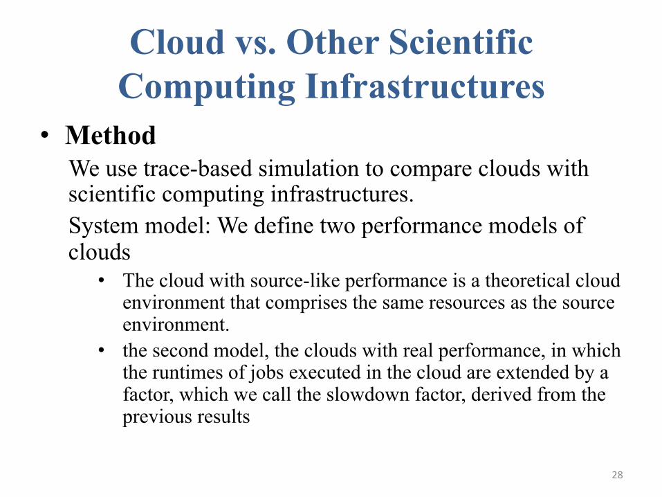
Cloud vs. Other Scientific Computing Infrastructures

•  Method We use trace-based simulation to compare clouds with scientific computing infrastructures. System model: We define two performance models of clouds •  The cloud with source-like performance is a theoretical cloud

environment that comprises the same resources as the source environment.

•  the second model, the clouds with real performance, in which the runtimes of jobs executed in the cloud are extended by a factor, which we call the slowdown factor, derived from the previous results

28

•  Job execution model: We assume exclusive resource use: for each job in the trace, the necessary resources are acquired from the cloud, then released after the job has been executed.

•  System workloads: the performance for both complete workloads, and MTC workloads are studied

•  Performance metrics: –  wait time (WT) –  response time (ReT) –  bounded slowdown (BSD)=max(1,ReT/max(10,ReT −WT))

where 10 is the bound that eliminates the bias of jobs with runtime below 10 seconds.

•  Cost metrics: the number of instance-hours used to complete all the jobs in the workload. This value can be converted directly into the cost for executing the whole workload for $/CPU-hour.

29

Experimental Setup

•  System setup: DGSim simulator, extended with two cloud models (theoretical and real) is used.

•  Workload setup: The same workload as that used for cloud performance evaluation is used (refer: slide no. 9).

30

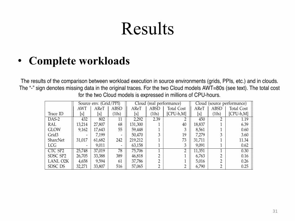
Results

•  Complete workloads

31

IEEE TPDS, MANY-TASK COMPUTING, NOVEMBER 2010 12TABLE 10

The results of the comparison between workload execution in source environments (grids, PPIs, etc.) and in clouds.The “-” sign denotes missing data in the original traces. For the two Cloud models AWT=80s (see text). The total cost

for the two Cloud models is expressed in millions of CPU-hours.Source env. (Grid/PPI) Cloud (real performance) Cloud (source performance)

AWT AReT ABSD AReT ABSD Total Cost AReT ABSD Total CostTrace ID [s] [s] (10s) [s] (10s) [CPU-h,M] [s] (10s) [CPU-h,M]DAS-2 432 802 11 2,292 2.39 2 450 2 1.19RAL 13,214 27,807 68 131,300 1 40 18,837 1 6.39GLOW 9,162 17,643 55 59,448 1 3 8,561 1 0.60Grid3 - 7,199 - 50,470 3 19 7,279 3 3.60SharcNet 31,017 61,682 242 219,212 1 73 31,711 1 11.34LCG - 9,011 - 63,158 1 3 9,091 1 0.62CTC SP2 25,748 37,019 78 75,706 1 2 11,351 1 0.30SDSC SP2 26,705 33,388 389 46,818 2 1 6,763 2 0.16LANL O2K 4,658 9,594 61 37,786 2 1 5,016 2 0.26SDSC DS 32,271 33,807 516 57,065 2 2 6,790 2 0.25

0

10

20

0.1 1 2 3 4 5 6 7 0

0.5

1

Ave

rag

e R

esp

on

se

Tim

e [

m]

To

tal C

ost

[Cp

u-H

,M]

Slowdown Factor

Avg. Response TimeAvg. Cost

0

10

20

2 3 4 5 6 7 8 9 10 0

0.5

1

Ave

rag

e R

esp

on

se

Tim

e [

m]

To

tal C

ost

[Cp

u-H

,M]

Slowdown Factor


Fig. 7. Performance and cost of using cloud resources for MTC workloads with various slowdown factors for sequentialjobs (left), and parallel jobs(right) using the DAS-2 trace.

the cloud (see Section 5.1). In previous sections, we haveused a slowdown factor of 7 for sequential jobs, and10 for parallel jobs for modeling clouds with real per-formance. We now evaluate the performance of cloudswith real performance using only the MTC workloadswith various slowdown factors for both sequential andparallel jobs. Similar to previous section, when extractingthe MTC workload from complete workloads we assumethat a user is an MTC user if B ! 1, 000 and J ! 10, 000.

Figure 7 shows the average response time and costof clouds with real performance with various slowdownfactors for sequential (left) and parallel (right) jobs usingthe DAS-2 trace. As the slowdown factor increases, weobserve a steady but slow increase in cost and responsetime for both sequential and parallel jobs. This is ex-pected: the higher the response time, the longer a cloudresource is used, increasing the total cost. The sequentialjobs dominate the workload both in number of jobs andin consumed CPU time, and their average response timeincreases linearly with the performance slowdown; thus,

TABLE 12Relative strategy performance: resource bulk allocation(S2) vs. resource acquisition and release per job (S1).Only performance differences above 5% are shown.

Relative Cost DAS-2 Grid3 LCG LANL O2K|S2!S1|

S1! 100 [%] 30.2 11.5 9.3 9.1

improving the performance of clouds for sequential jobsshould be the first priority of cloud providers.

5.3.4 Performance and Security vs. CostCurrently, clouds lease resources but do not offer aresource management service that can use the leasedresources. Thus, the cloud adopter may use any of theresource management middleware from grids and PPIs;for a review of grid middleware we refer to our recentwork [55]. We have already introduced the basic con-cepts of cloud resource management in Section 4.2, andexplored the potential of a cloud resource managementstrategy (strategy S1) for which resources are acquired

TABLE 11The results of the comparison between workload execution in source environments (grids, PPIs, etc.) and in cloudswith only the MTC part extracted from the complete workloads. The LCG, CTC SP2, SDSC SP2, and SDSC DS

traces are not presented, as they do not have enough MTC users (the criterion is described in text).Source env. (Grid/PPI) Cloud (real performance) Cloud (source performance)

AWT AReT ABSD AReT ABSD Total Cost AReT ABSD Total CostTrace ID [s] [s] (10s) [s] (10s) [CPU-h,M] [s] (10s) [CPU-h,M]DAS-2 70 243 3 776 2 0.65 252 2 0.61RAL 4,866 18,694 24 68,847 1 6.60 17,272 1 1.80GLOW 6,062 13,396 41 29,416 1 1.40 7,413 1 0.42Grid3 - 7,422 - 29,769 4 10.61 7,502 4 3.30SharcNet 10,387 30,092 6 141,510 1 7.10 20,182 1 1.09LANL O2K 635.78 1,715 4 94 2 0.10 1,171 1 <0.01

Results

•  An order of magnitude better performance is needed for clouds to be useful for daily scientific computing.

•  Price-wise, clouds are reasonably cheap for scientific computing, if the usage and funding scenarios allow it (but usually they do not).

•  Clouds are now a viable alternative for short deadlines.

32

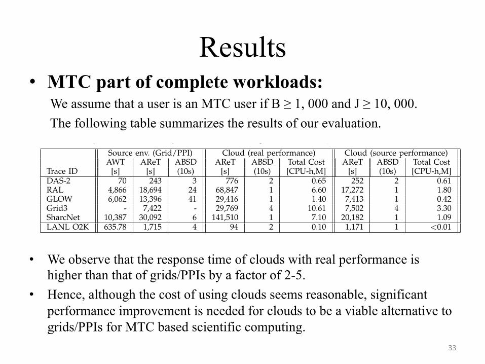
Results •  MTC part of complete workloads:

We assume that a user is an MTC user if B ≥ 1, 000 and J ≥ 10, 000. The following table summarizes the results of our evaluation.

•  We observe that the response time of clouds with real performance is higher than that of grids/PPIs by a factor of 2-5.

•  Hence, although the cost of using clouds seems reasonable, significant performance improvement is needed for clouds to be a viable alternative to grids/PPIs for MTC based scientific computing.

33





0

10

20

0.1 1 2 3 4 5 6 7 0

0.5

1

Ave

rage R

esp

onse

Tim

e [m

]

Tota

l Cost

[C

pu-H

,M]

Slowdown Factor


0

10

20

2 3 4 5 6 7 8 9 10 0

0.5

1

Ave

rage R

esp

onse

Tim

e [m

]

Tota

l Cost

[C

pu-H

,M]

Slowdown Factor







S1! 100 [%] 30.2 11.5 9.3 9.1






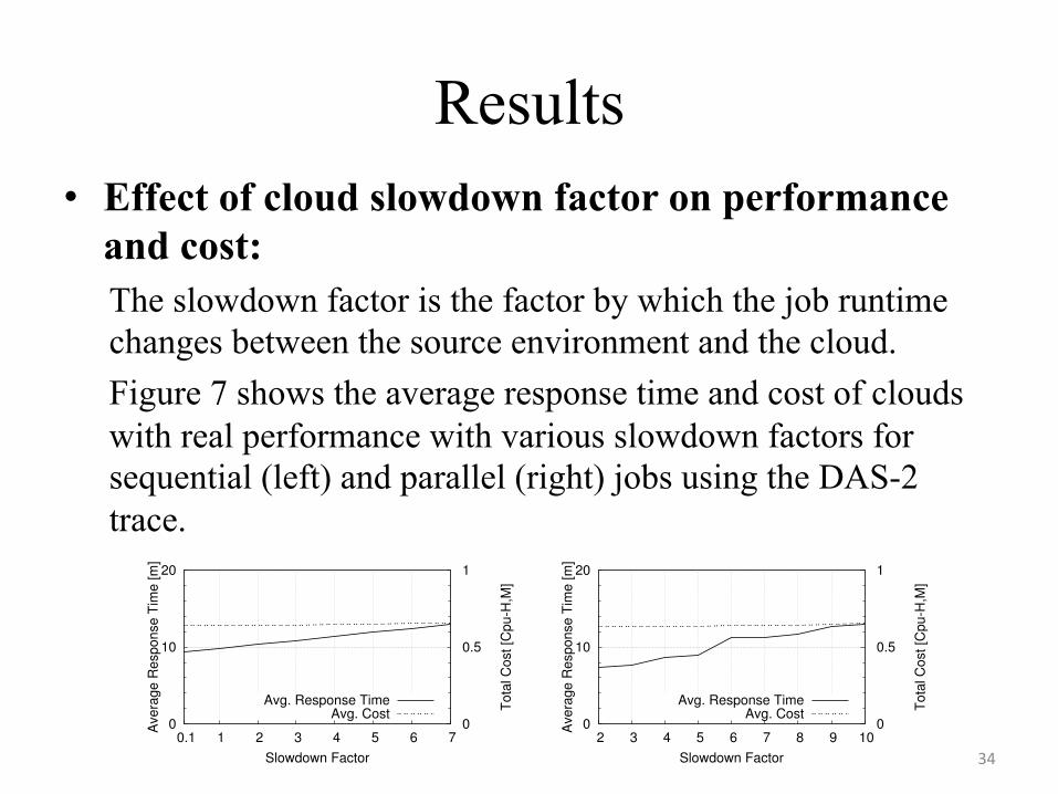
Results •  Effect of cloud slowdown factor on performance

and cost: The slowdown factor is the factor by which the job runtime changes between the source environment and the cloud. Figure 7 shows the average response time and cost of clouds with real performance with various slowdown factors for sequential (left) and parallel (right) jobs using the DAS-2 trace.

34





0

10

20

0.1 1 2 3 4 5 6 7 0

0.5

1

Ave

rag

e R

esp

on

se T

ime

[m

]

To

tal C

ost

[C

pu

-H,M

]

Slowdown Factor


0

10

20

2 3 4 5 6 7 8 9 10 0

0.5

1A

vera

ge

Re

spo

nse

Tim

e [

m]

To

tal C

ost

[C

pu

-H,M

]

Slowdown Factor







S1! 100 [%] 30.2 11.5 9.3 9.1






Results •  As the slowdown factor increases, we observe a steady but

slow increase in cost and response time for both sequential and parallel jobs.

•  This is expected: the higher the response time, the longer a cloud resource is used, increasing the total cost.

•  The sequential jobs dominate the workload both in number of jobs and in consumed CPU time, and their average response time increases linearly with the performance slowdown; thus, improving the performance of clouds for sequential jobs should be the first priority of cloud providers.

35

Results •  Performance and security vs. cost:

Strategy S1: resources are acquired and released for each submitted job. This strategy has good security and resource setup flexibility, but may incur high time and cost overheads, as resources that could otherwise have been reused are released as soon as the job completes. Strategy S2: resources are allocated in bulk for all users, and released only when there is no job left to be served The maximum relative cost difference between the strategies is for these traces around 30% .

36

Conclusion

•  The compute performance of the tested clouds is low.

•  While current cloud computing services are insufficient for scientific computing at large, they may still be a good solution for the scientists who need resources instantly and temporarily.

37

References •  Amazon Inc., “Amazon Elas+c Compute Cloud (Amazon

EC2),” Dec 2008, [Online] Available: hip://aws.amazon.com/ec2/.

•  GoGrid, “GoGrid cloud-‐server hos+ng,” Dec 2008, [Online] Available: hip://www.gogrid.com.

•  L. McVoy and C. Staelin, “LMbench -‐ tools for performance anal-‐ ysis,” [Online] Available: hip://www.bitmover.com/lmbench/,Dec 2008.

•  T. Bray, “Bonnie,” 1996, [Online] Available: hip://www.textuality.com/bonnie/, Dec 2008.

•  The HPCC Team , “HPCChallenge results,” Jan. 2009, [Online]. Available: hip://icl.cs.utk.edu/hpcc/hpcc results.cgi.

38

References

39

THANK YOU

40

Date post:	13-Feb-2017
Category:	Documents
Upload:	dominh
View:	215 times
Download:	0 times

Performance Analysis of Cloud Computing Services for Many-Tasks ...

Documents