Page 1
PERFORMANCE ANALYSIS OF ELLIPTIC CURVE MULTIPLICATION ALGORITHMS FOR ELLIPTIC CURVE CRYPTOGRAPHY
A THESIS SUBMITTED TO THE GRADUATE SCHOOL OF NATURAL AND APPLIED SCIENCES
OF MIDDLE EAST TECHNICAL UNIVERSITY
BY
AYÇA BAHAR ÖZCAN
IN PARTIAL FULFILLMENT OF THE REQUIREMENTS FOR
THE DEGREE OF MASTER OF SCIENCE IN
ELECTRICAL AND ELECTRONICS ENGINEERING
SEPTEMBER 2006
Page 2
ii
Approval of the Graduate School of Natural and Applied Sciences
_______________________ Prof. Dr. Canan Özgen
Director I certify that this thesis satisfies all the requirements as a thesis for the degree of Master of Science.
________________________ Prof. Dr. İsmet Erkmen
Head of Department This is to certify that we have read this thesis and that in our opinion it is fully adequate, in scope and quality, as a thesis for the degree of Master of Science. __________________________ Assoc. Prof. Dr. Melek D. Yücel
Supervisor Examining Committee Members Prof. Dr. Rüyal Ergül (METU, EEE) ________________ Assoc. Prof. Dr. Melek D. Yücel (METU, EEE) ________________ Prof. Dr. Kemal Leblebicioğlu (METU, EEE) ________________
Prof. Dr. Ersan Akyıldız (METU, MATH) ________________ Assoc. Prof. Dr. Ali Doğanaksoy (METU, MATH) ________________
Page 3
iii
I hereby declare that all information in this document has been obtained and
presented in accordance with academic rules and ethical conduct. I also declare
that, as required by these rules and conduct, I have fully cited and referenced all
material and results that are not original to this work.
Name, Last Name: Ayça Bahar ÖZCAN
Signature:
Page 4
iv
ABSTRACT
PERFORMANCE ANALYSIS OF ELLIPTIC CURVE MULTIPLICATION ALGORITHMS FOR ELLIPTIC CURVE CRYPTOGRAPHY
Özcan, Ayça Bahar
M.Sc., Department of Electrical and Electronics Engineering
Supervisor: Assoc. Prof. Dr. Melek D. Yücel
September 2006, 83 pages
Elliptic curve cryptography (ECC) has been introduced as a public-key
cryptosystem, which offers smaller key sizes than the other known public-key
systems at equivalent security level. The key size advantage of ECC provides
faster computations, less memory consumption, less processing power and
efficient bandwidth usage. These properties make ECC attractive especially for
the next generation public-key cryptosystems. The implementation of ECC
involves so many arithmetic operations; one of them is the elliptic curve point
multiplication operation, which has a great influence on the performance of ECC
protocols.
In this thesis work, we have studied on elliptic curve point multiplication
methods which are proposed by many researchers. The software implementations
of these methods are developed in C programming language on Pentium 4 at 3
GHz. We have used NIST-recommended elliptic curves over prime and binary
fields, by using efficient finite field arithmetic. We have then applied our elliptic
curve point multiplication implementations to Elliptic Curve Digital Signature
Page 5
v
Algorithm (ECDSA), and compared different methods. The timing results are
presented and comparisons with recent studies have been done.
Keywords: Elliptic Curve Cryptography, Elliptic Curve Point Multiplication,
Prime Field, Binary Field, Software Implementation
Page 6
vi
ÖZ
ELİPTİK EĞRİ KRİPTOGRAFİSİNDE KULLANILAN ÇARPMA
ALGORİTMALARININ BAŞARIM ÇÖZÜMLEMESİ
Özcan, Ayça Bahar
Yüksek Lisans, Elektrik ve Elektronik Mühendisliği Bölümü
Tez yöneticisi: Doç. Dr. Melek D. Yücel
Eylül 2006, 83 sayfa
Eliptik eğri kriptografisi (EEK), aynı güvenlik seviyesinde diğer asimetrik
anahtar kripto sistemlerinden daha kısa anahtar boyları gerektiren bir asimetrik
anahtar kripto sistemi olarak önerilmiştir. Anahtar boyunun kısalığı, hızlı
hesaplamalar, daha az bellek alanı gereksinimi, daha az işlem gücü ve bant
genişliği verimliliği sağlar. Yeni nesil asimetrik anahtar kripto sistemlerinde,
EEK sahip olduğu bu özellikleriyle ilgi odağı olmuştur. EEK uygulaması birçok
aritmetik işlemden oluşmaktadır. Eliptik eğri noktası çarpma işlemi bu
işlemlerden biridir ve kripto protokollerindeki işlem hızında en etkin olanıdır.
Bu çalışmada, birçok araştırmacı tarafından önerilmiş eliptik eğri nokta
çarpma metodları incelenmiştir. Bu metodların C programlama dilinde, 3 GHz’lik
Pentium 4 işlemci üzerinde yazılım uygulaması yapılmıştır. Uygulamalarda NIST
tarafından tavsiye edilien, asal ve ikili alanlarda tanımlanmış eliptik eğriler
kullanılmıştır. Uygulaması yapılan eliptik eğri nokta çarpma metotları, Eliptik
Eğri Sayısal İmza Algoritması’nda kullanılmış ve değişik metotlar
Page 7
vii
karşılaştırılmıştır. Elde edilen zaman değerleri, son zamanlarda yapılan
çalışmalarla karşılaştırılmıştır.
Anahtar sözcükler: Eliptik Eğri Kriptografisi, Eliptik Eğri Nokta Çarpma
İşlemi, Asal Alan, İkili Alan, Yazılım Uygulama.
Page 8
viii
To my parents, Gülsen & Mahmut Acımış
Page 9
ix
ACKNOWLEDGEMENTS
I would like to express my sincere appreciation to my advisor, Assoc.
Prof. Dr. Melek Yücel for her encouragement and support in every stage of this
research.
I would like to give special thanks to my colleagues for their
encouragement and support.
I would like to express my deep gratitude to all who have encouraged and
helped me at the different stages of this work.
My sister and my parents, I thank them for everything.
Finally, I wish to express my thanks to ASELSAN Inc. for the facilities
provided.
Page 10
x
TABLE OF CONTENTS
ABSTRACT ................................................................................................................................... IV
ÖZ .................................................................................................................................................. VI
ACKNOWLEDGEMENTS ........................................................................................................... IX
LIST OF TABLES .......................................................................................................................XIII
LIST OF FIGURES..................................................................................................................... XIV
LIST OF ABBREVIATIONS .......................................................................................................XV
CHAPTER
1. INTRODUCTION........................................................................................................................ 1
2. PUBLIC-KEY CRYPTOGRAPHY AND ELLIPTIC CURVES................................................. 3 2.1 CRYPTOGRAPHY FUNDAMENTALS.............................................................................. 3
2.2 USING PUBLIC-KEY CRYPTOSYTEMS.......................................................................... 4 2.2.1 Encryption and decryption (confidentiality) .................................................................. 5 2.2.2 Digital signatures (authentication, integrity, non-repudiation) ...................................... 5
2.3 MATHEMATICAL PROBLEMS FOR PUBLIC-KEY CRYPTOSYSTEMS ..................... 6 2.3.1 Discrete Logarithm Problem (DLP)............................................................................... 6 2.3.2 Elliptic Curve Discrete Logarithm Problem (ECDLP) .................................................. 7
2.4 WHY ELLIPTIC CURVE CRYPTOGRAPHY? .................................................................. 7 2.4.1 Security .......................................................................................................................... 8 2.4.2 Efficiency....................................................................................................................... 8
2.5. ELLIPTIC CURVE ARITHMETIC..................................................................................... 9 2.5.1 Elliptic curve definition ............................................................................................... 10 2.5.2 Group law for elliptic curves ....................................................................................... 13 2.5.3 Point representation ..................................................................................................... 16 2.5.4 Point multiplication...................................................................................................... 18
3. FIELD ARITHMETIC AND ELLIPTIC CURVE POINT MULTIPLICATION...................... 19 3.1 FINITE FIELD ARITHMETIC........................................................................................... 19
3.1.1 Finite field arithmetic in prime fields........................................................................... 20
Page 11
xi
3.1.2 Finite field arithmetic in binary fields.......................................................................... 21 3.1.3 Field arithmetic on Pentium processor........................................................................ 23
3.2 DESCRIPTION OF ELLIPTIC CURVE POINT MULTIPLICATION OPERATION
ALGORITHMS......................................................................................................................... 25 3.2.1 Point P is unknown ...................................................................................................... 26 3.2.2 Window Methods......................................................................................................... 28 3.2.3 Point P is known .......................................................................................................... 32
3.3 PERFORMANCE COMPARISON OF ELLIPTIC CURVE POINT MULTIPLICATION
METHODS................................................................................................................................ 35 3.3.1 EC point multiplication over Prime Fields................................................................... 35 3.2.2 EC point multiplication over Binary Fields ................................................................. 44
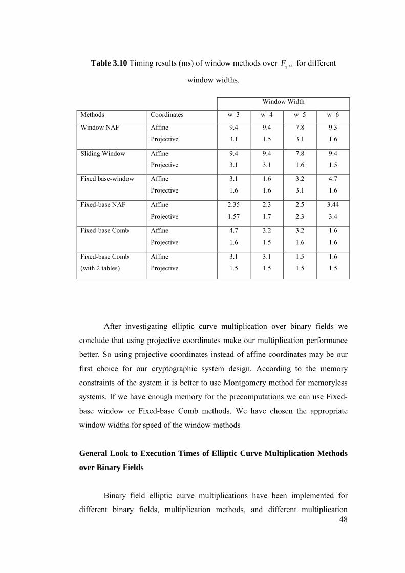
3.4 COMMENTS ON ELLIPTIC CURVE MULTIPLICATION IMPLEMENTATIONS...... 50
4. ELLIPTIC CURVE DIGITAL SIGNATURE ALGORITHM (ECDSA) .................................. 53 4.1 SIGNATURE SCHEMES AND ECDSA DESCRIPTION................................................. 53
4.2 IMPLEMENTING ECDSA SIGNATURE GENERATION AND VERIFICATION
ALGORITHMS......................................................................................................................... 56
5. CONCLUSION .......................................................................................................................... 60
REFERENCES............................................................................................................................... 62
APPENDICES
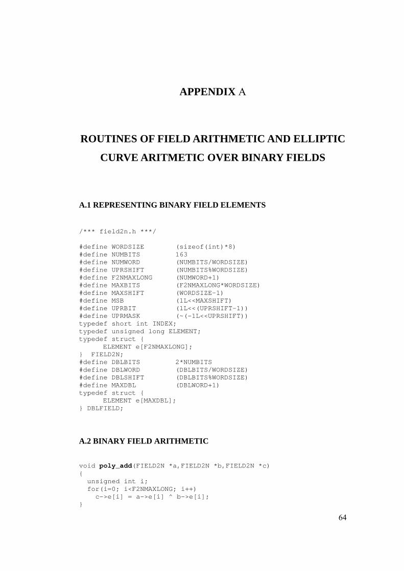
A. ROUTINES OF FIELD ARITHMETIC AND ELLIPTIC CURVE ARITMETIC OVER BINARY FIELDS .......................................................................................................................... 64
A.1 REPRESENTING BINARY FIELD ELEMENTS............................................................. 64
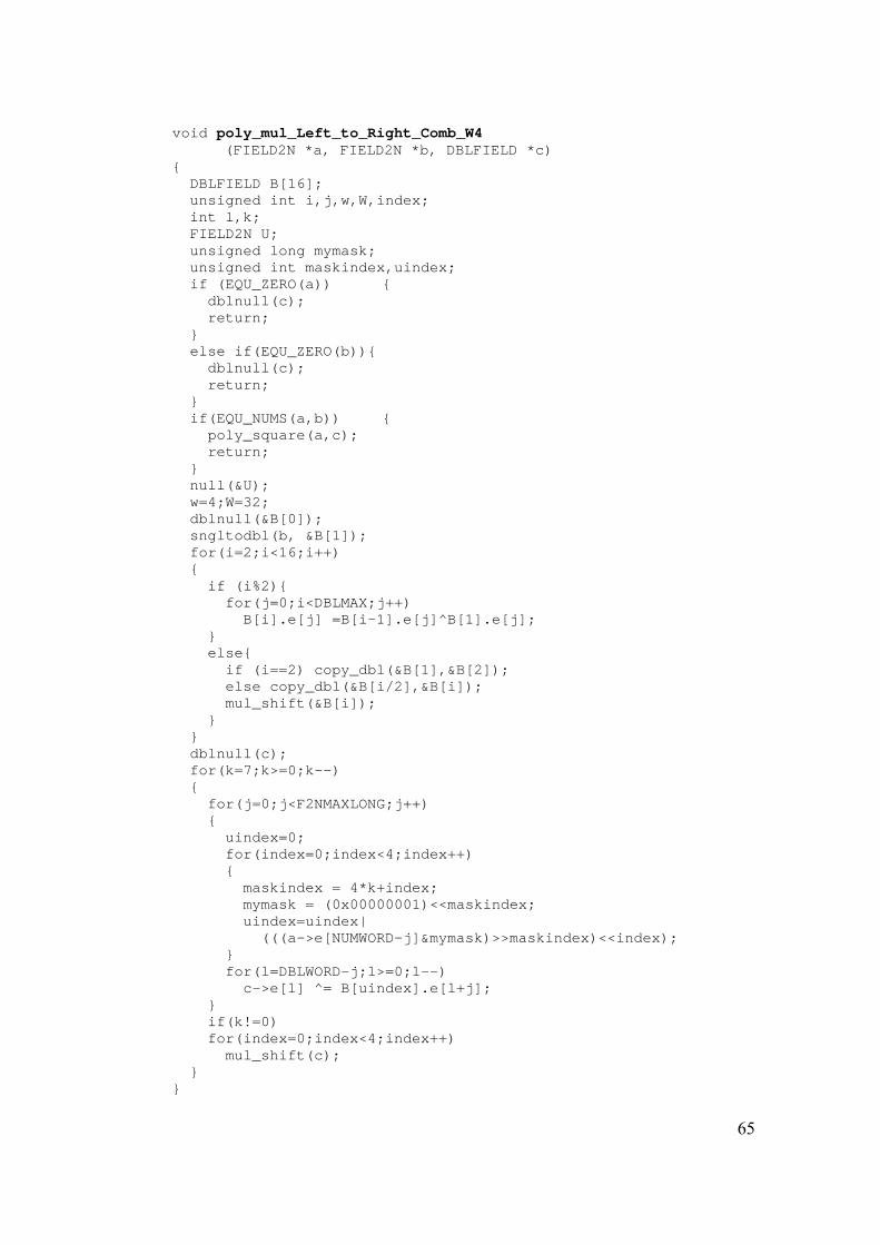
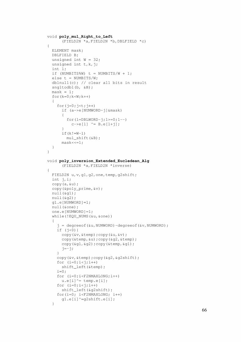
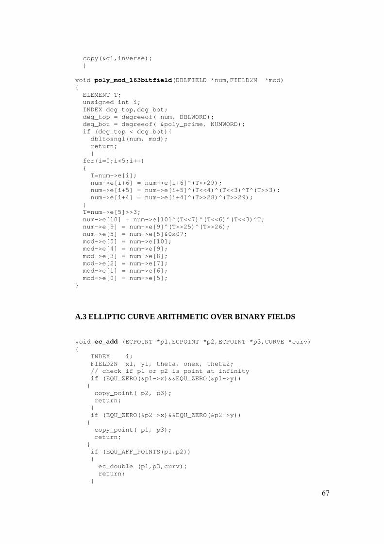
A.2 BINARY FIELD ARITHMETIC ....................................................................................... 64
A.3 ELLIPTIC CURVE ARITHMETIC OVER BINARY FIELDS......................................... 67
B. ROUTINES OF FIELD ARITHMETIC AND ELLIPTIC CURVE ARITHMETIC OVER PRIME FIELDS ............................................................................................................................. 72
B.1 REPRESENTING PRIME FIELD ELEMENTS................................................................ 72
B.2 PRIME FIELD ARITHMETIC........................................................................................... 72
B.3 ELLIPTIC CURVE ARITHMETIC ................................................................................... 74
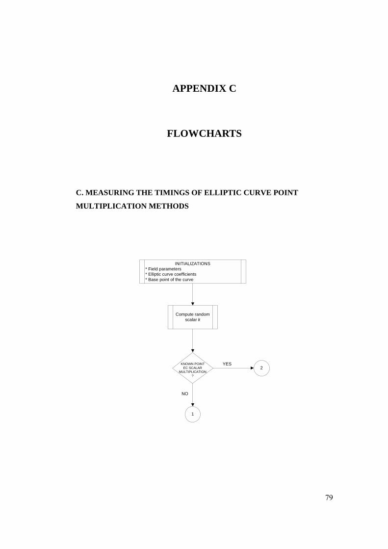
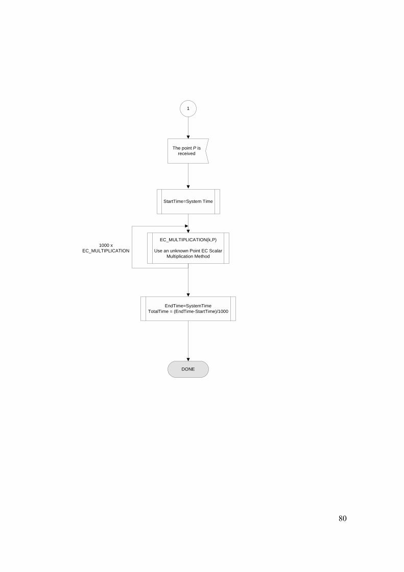
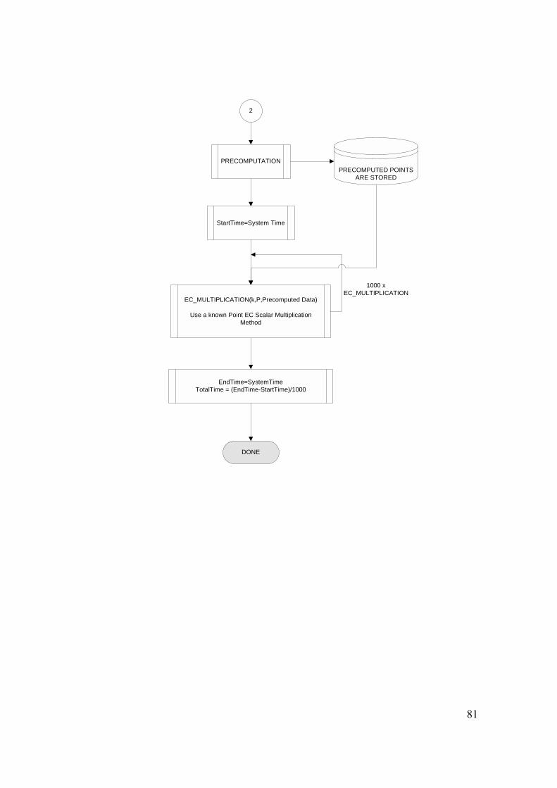
C. FLOWCHARTS ........................................................................................................................ 79 C.1 MEASURING THE TIMINGS OF ELLIPTIC CURVE POINT MULTIPLICATION
METHODS................................................................................................................................ 80
Page 12
xii
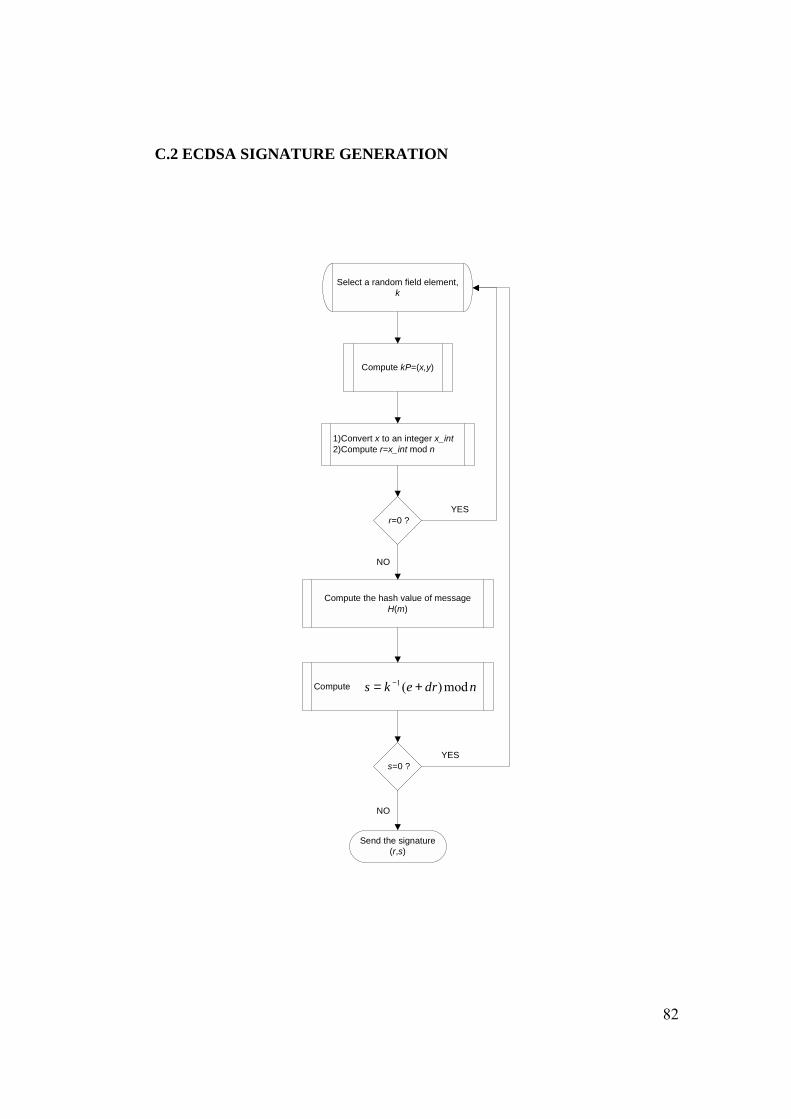
C.2 ECDSA SIGNATURE GENERATION ............................................................................. 83
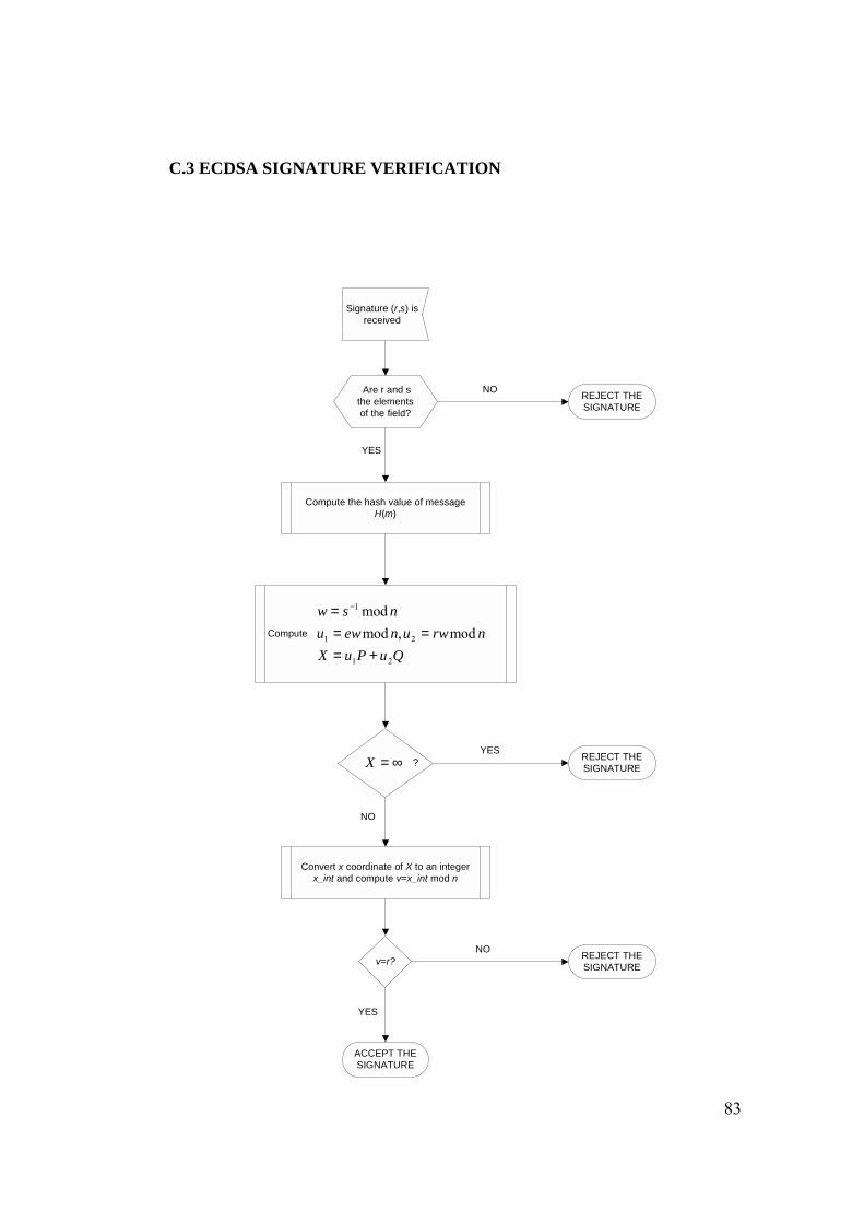
C.3 ECDSA SIGNATURE VERIFICATION ........................................................................... 83
Page 13
xiii
LIST OF TABLES
TABLES 2.1 RSA, DSA and ECC key sizes for equivalent security levels. ................................................... 9
3.1 Execution time (µs) of field operations in 192 224 256 384 521, , , ,F F F F F . .................................. 24
3.2 Execution time (µs) of field operations in 163 283 4092 2 2, ,F F F ................................................... 25
3.3 NIST-recommended randomly chosen elliptic curves over prime fields
1 9 2 2 2 4 2 5 6 3 8 4 5 2 1, , , ,F F F F F . .................................................................................. 36
3.4 Timing results (ms) of Right-to-Left, Left-to- Right and Binary NAF methods for elliptic
curve point multiplication over prime fields. ........................................................................ 38 3.5 Number of stored EC point data for window methods. ............................................................ 39
3.6 Timing results (ms) of window methods over 224F for different window widths. .................. 41
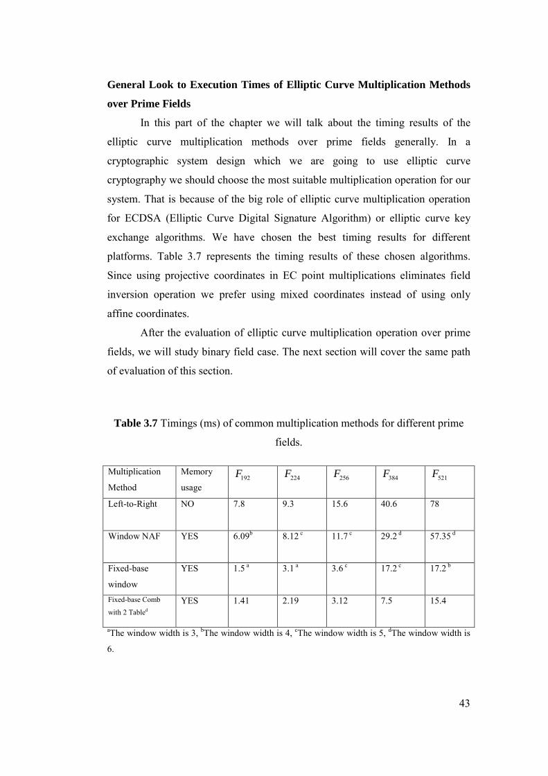
3.7 Timings (ms) of common multiplication methods for different prime fields. .......................... 43
3.8 NIST-recommended elliptic curves over 163 233 409283 5712 2 2, , , ,F F F F F . ................................... 45
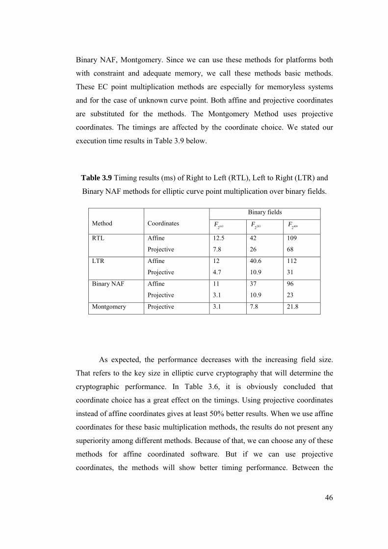
3.9 Timing results (ms) of Right to Left (RTL), Left to Right (LTR) and Binary NAF methods for
elliptic curve point multiplication over binary fields. ........................................................... 46
3.10 Timing results (ms) of window methods over 1632F for different window widths................. 48
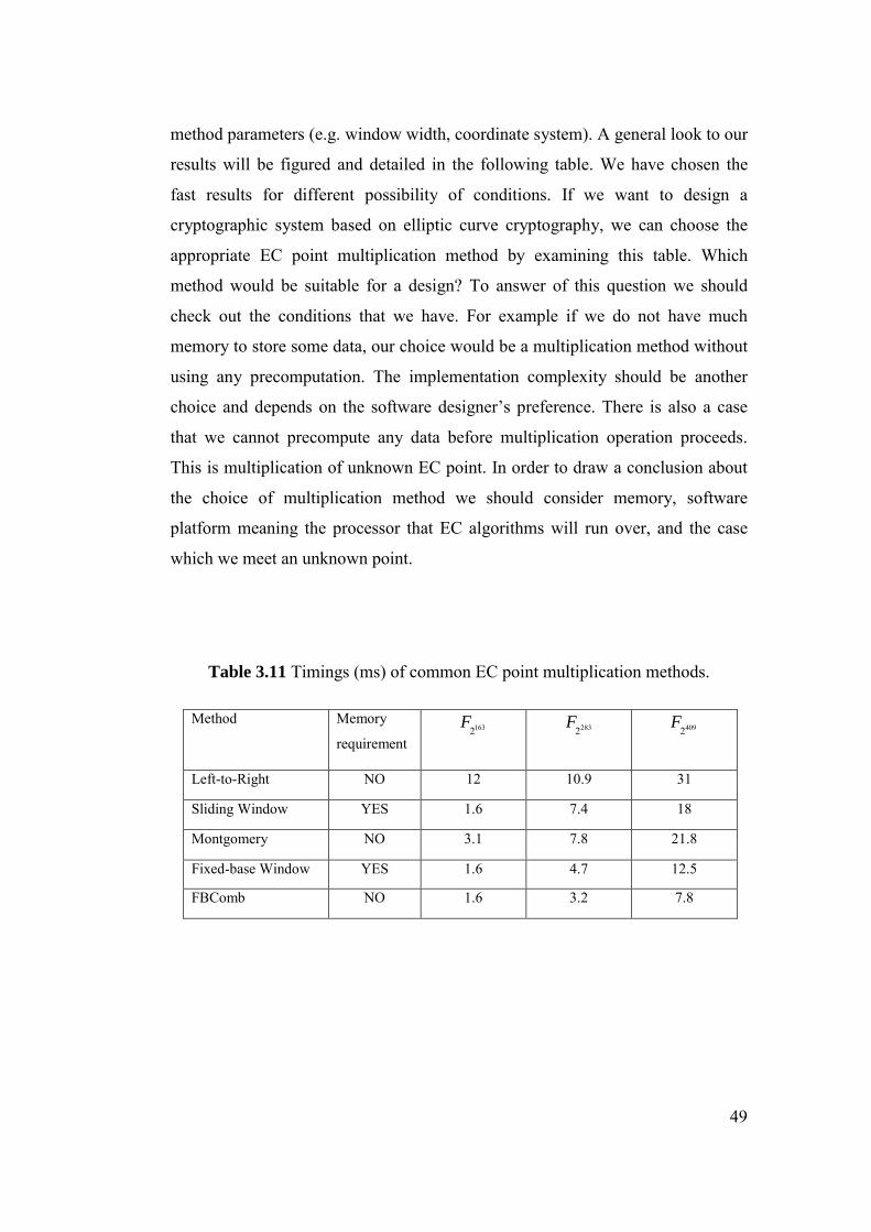
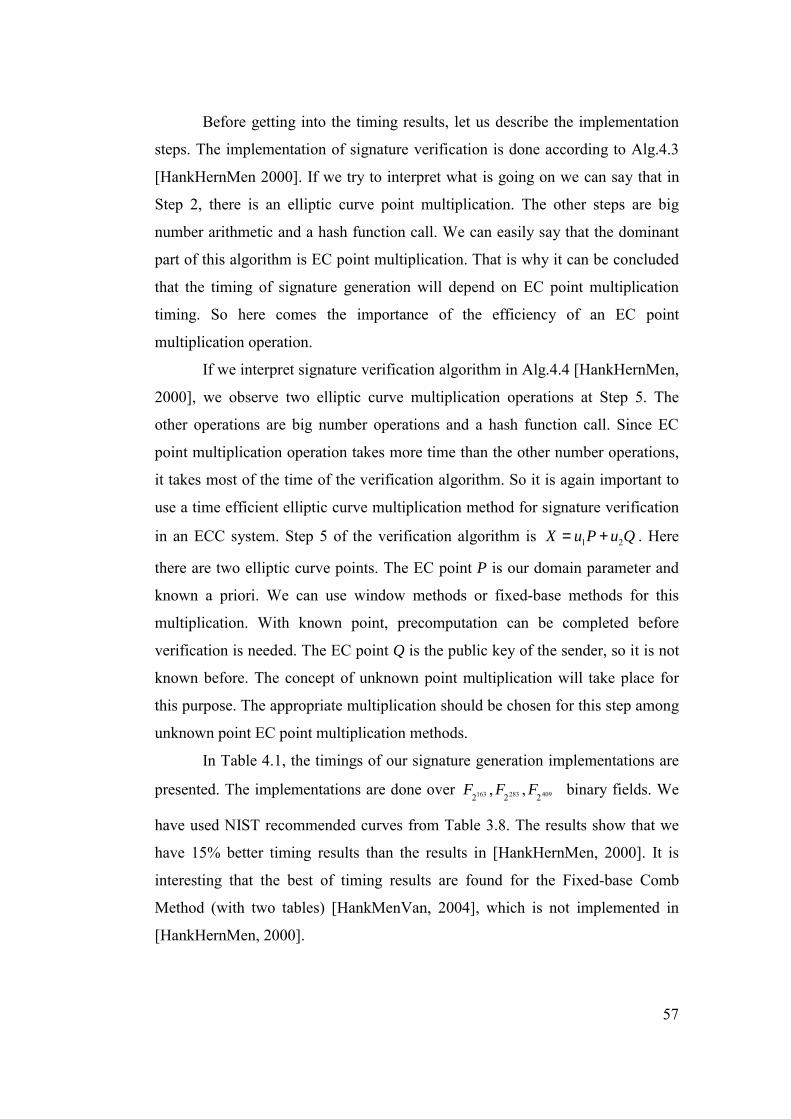
3.11 Timings (ms) of common EC point multiplication methods. ................................................. 49 4.1. Timings (ms) of ECDSA signature generation algorithm with different elliptic curve
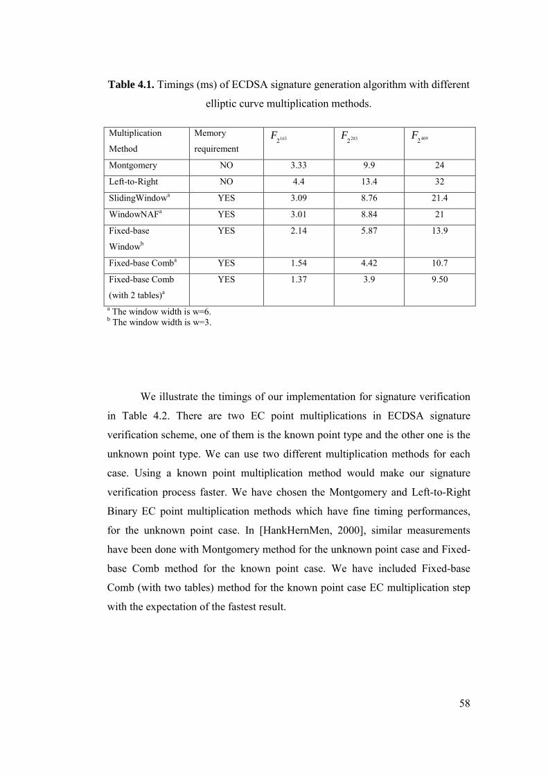
multiplication methods.......................................................................................................... 58 4.2 Timings (ms) of ECDSA signature verification algorithm with different elliptic curve
multiplication methods.......................................................................................................... 59
Page 14
xiv
LIST OF FIGURES
FIGURES
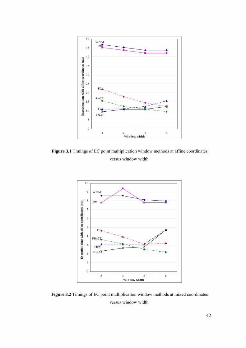
2.1 Elliptic curves over R . ............................................................................................................. 11 2.2 Geometric addition of elliptic curve points, P+Q=R. .............................................................. 13 2.3 Geometric doubling of elliptic curve point, 2P=R.................................................................... 14 3.1 Timings of EC point multiplication window methods at affine coordinates versus window
width. .................................................................................................................................... 42 3.2 Timings of EC point multiplication window methods at mixed coordinates versus window
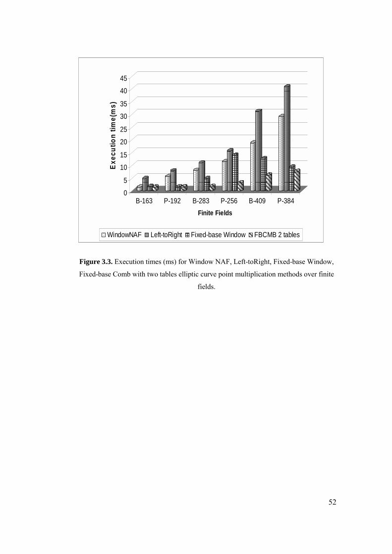
width. .................................................................................................................................... 42 3.3. Execution times (ms) for Window NAF, Left-toRight, Fixed-base Window, Fixed-base Comb
with two tables elliptic curve point multiplication methods over finite fields. ..................... 52
Page 15
xv
LIST OF ABBREVIATIONS
AES Advanced Encryption Standard
DES Data Encryption Standard
DL Discrete Logarithm
DLP Discrete Logarithm Problem
DSA Digital Signature Algorithm
EC Elliptic Curve
ECC Elliptic Curve Cryptography
ECDLP Elliptic Curve Discrete Logarithm Problem
ECDSA Elliptic Curve Digital Signature Algorithm
FIPS Federal Information Processing Standards
IFP Integer Factorization Problem
NAF Non-Adjacent Form
NIST National Institute of Standards and Technology
RSA Rivest-Shamir-Adleman
Page 16
1
CHAPTER 1
INTRODUCTION
For over a hundred years, mathematicians have studied elliptic curves. In
1985, elliptic curves were used independently by Neal Koblitz [Kob, 1987] and
Victor Miller [Mil, 1986] to design public key cryptographic systems. Their
proposal was using the group of points on an elliptic curve (EC) defined over a
finite field to implement discrete log cryptosystems. Since then lots of research
have been published on the security and efficient implementation of elliptic curve
cryptography. In the late 1990, elliptic curve systems started receiving
commercial acceptance. Standard organizations specified elliptic curve protocols
and private companies included these protocols in their security products. When
we compare the traditional public-key cryptographic algorithms, elliptic curve
cryptography algorithms can achieve the same level of security with shorter key
lengths. The shorter key lengths provide speed, less memory usage and less
energy consumption for a cryptosystem. That is why elliptic curve cryptography
has become a challenging interest for many researchers.
Since elliptic curve cryptography aspects are based on EC point
multiplication operation, we focused on EC point multiplication methods. This
thesis study has covered many elliptic curve multiplication methods, published
until now [HanMenVan, 2004], [BrHankLopMen, 2001], [HankHernMen, 2000].
In this work, software implementations of Right-to-Left Binary, Left-to-Right
Binary, Binary NAF (Non-Adjacent Form), Window NAF, Sliding Window,
Montgomery, Fixed-base Window, Fixed-base NAF, Fixed-base Comb, and
Fixed-base Comb (with two tables) methods have been done on Pentium 4
processor at 3 GHz and their performances have been measured. We have
developed the EC point multiplication algorithms both for prime and binary
Page 17
2
fields. The main performance criterion is the speed of the algorithms, which is
affected by the choice of the field, the methods used in performing the field
operations, the coordinate system for EC point multiplication algorithms, and the
algorithm parameters such as window width. We have optimized the speed
performances of these EC point multiplication methods by suitable choice of the
field arithmetic methods, point representation and window width of the
algorithms. The comparisons of EC point multiplication methods, their
superiority to each other and behavior according to the chosen field have been
discussed.
The organisation of this thesis is as follows. Chapter 2 begins with the
general overview of public-key cryptosystems. Then elliptic curve arithmetic is
described, definitions and descriptions of the basic elliptic curve operations are
stated [HankMenVan, 2004].
In Chapter 3, the description of the field arithmetic is given
[HankHernMen, 2000], [BrHankLopMen, 2001]. The arithmetic operations and
algorithms differ according to the binary field or prime field choice. EC point
multiplication implementations are based on field operations. This chapter
presents the performances of the implemented field operations. We continue by
focusing on EC point multiplication operation. The algorithms are described
theoretically in detail [HankMenVan, 2004]. We have implemented the EC point
multiplication methods in C code according to these descriptions. The
performance of the implementations have been measured and the results have
been stated together with comparisons to the previous researches
[BrHankLopMen, 2001], [HankHernMen, 2000], [YanShi, 2006].
In Chapter 4, the chosen EC point multiplication methods are applied to
the signature generation and verification of Elliptic Curve Digital Signature
Algorithm (ECDSA) and implementation timings are illustrated.
Chapter 5 presents the conclusions of this thesis work.
Page 18
3
CHAPTER 2
PUBLIC-KEY CRYPTOGRAPHY AND ELLIPTIC
CURVES
2.1 CRYPTOGRAPHY FUNDAMENTALS
The general definition of cryptography is the design and analysis of
mathematical techniques that enable secure communications in the existence of
adversaries. We can model the communication media for many different cases.
For example, communication can be between two people via a cellular telephone
network, or the communication between a web browser and a web site, or
sending an email message to someone over the internet, or between a smart card
and a computer. All these examples are vulnerable to eavesdrop. In today’s world
any communication scenario brings the requirement of security.
In a cryptographic communication system, we need to provide some
fundamental aspects for secure communications given as follows:
1. Confidentiality
2. Data Integrity
3. Data origin authentication
4. Entity authentication
5. Non-repudiation
Symmetric-key Cryptography
In a symmetric-key cryptographic system, the entities first agree upon the
keying material. Keying material should be secret and authentic. A symmetric-
Page 19
4
key encrytion scheme is used (i.e., DES, RC4, AES,..etc) for data achievement,
data origin authentication, and message authentication codes. The major
advantage of the symmetric-key cryptography is its high efficiency. However
there exist significant drawbacks. One of them is the key distribution problem.
Key distribution should be handled secretly and in authenticated form. The
second drawback is the key management problem. In a network, cryptopraphic
system can work only with different keying materials for each entity.
Public-key Cryptography
Public-key schemes require only the communication entities exchange
keying material that is authentic but not secret. Each entity selects a single key
pair (e,d) which consist of a public key e and related private key d. The private
key is kept secret by the entity. The basic property of these keys is the
computational infeasibility of having the private key from the knowledge of the
public key. Public-key cryptography provides solutions to the problems of
symmetric-key cryptography, specifically key distribution, key management, and
the provision of non-repudiation.
Although we can eliminate the requirement for a secret channel for the
distribution of keys by using public-key cryptography, implementing public-key
infrastructure for distributing and managing public keys can be challenging in
practice. Furthermore, public-key operations are usually slower than their
symmetric-key counterparts. So, it is preferrable to use hybrid systems that
benefit from the efficiency of symmetric-key algorithms and functionality of
public-key algorithms.
2.2 USING PUBLIC-KEY CRYPTOSYTEMS
Public-key cryptosystems can provide all the services of information
security. In this section we will describe how these services could be supplied by
a public-key cryptosystem.
Page 20
5
2.2.1 Encryption and decryption (confidentiality)
Assume we want to send a message to one of our friends. We will use the
public key e of our friend to encrypt our message M. After encrypting the
message, it is converted to ciphertext C. Now we can send our ciphered message
C to our friend. The receiver will obtain the original message M by using his own
secret private key. Private key is secret so that only the owner can have the
enciphered message. Public-key encryption and decryption service the
confidentiality required for a cryptosystem.
To have the system confidentiality, the users should know the public keys
are authentic and belong to the specified users. At this point another concept is
introduced: Electronic or digital certificates which are distributed by a trusted
third party, should be used.
2.2.2 Digital signatures (authentication, integrity, non-repudiation)
Electronic form of handwritten signatures are called digital signatures.
Since it is easy to have a fake electronic signature it must be produced in a
systematic secure way. Public-key cryptographic systems are used for digital
signature schemes. The use of public-key systems in signature algorithms is
diferent than the use in encryption and decryption. Now let’s suppose a signature
requirement case where we want to sign a message M. First of all, we will
compute the hash value h(M) of the message by using a hash function. The
signature S of message M is obtained by encrypting the hash value h(M) with our
own private key, d. We can then send the message M together with the signature
S. After the message and the signature have been received, the receiver uses our
public key e to transform signature to the hash value. The verification occurs if
the recomputed hash value h(M) and the decrypted value of S are equal. If the
verification is completed with equality, the receiver accepts that our signature is
Page 21
6
valid. If the verification fails, the receiver understands that the signature is not
ours and the message is not accepted.
From the signature scenario, we can conclude that the public-key
signature scheme provides data origin authentication, data integrity and non-
repudiation.
2.3 MATHEMATICAL PROBLEMS FOR PUBLIC-KEY
CRYPTOSYSTEMS
The security level of a public-key cryptographic system is graded
according to the hardness of the mathematical problem underlying the
cryptographic algorithm. The commonly used public-key schemes provide their
security by the mathematical problems which are given as follows.
1. Integer factorization problem (IFP).
2. Discrete logarithm problem (DLP).
3. Elliptic curve discrete logarithm problem (ECDLP).
All these problems are extremely difficult to solve by today’s computing
power provided that the big numbers used are big enough . The hardness of the
integer factorization problem is essential for the security of RSA public-key
encryption and signature schemes. The security of ElGamal public-key
encryption and signature schemes and their variants such as Digital Signature
Algorithm (DSA) depends on the hardness of DLP. Elliptic curve cryptography
security depends on the intractibility of ECDLP. which is another form of classic
DLP. Because of this analogy we are going to mention both problems.
2.3.1 Discrete logarithm problem (DLP)
Let ),( ∗G be a multiplicative cyclic group of order p which is a prime. In
the cyclic group, addition and multiplication are performed modulo p. The
domain parameters are p, a given integer g ∈ G, the private key x randomly
Page 22
7
selected from the interval [ ]1,0 −p , and the public key is pgy x mod= . The
discrete logarithm problem modulo p is to determine the integer x for a given pair
of g, y and p. The integer x is called the discrete logarithm of y to the base g. The
known algorithms to solve the discrete logarithm problem modulo p are not
computationally efficient for large p.
2.3.2 Elliptic curve discrete logarithm problem (ECDLP)
Let p be a prime number and pF be the field of integers modulo p. Say,
the equation of a simple elliptic curve E over pF is
baxxy ++= 32 (1.1)
where pFba ∈, satisfy ≠+ 23 274 ba 0 (mod p). A pair pFyx ∈),( is a point on
the curve if ),( yx satisfies equation (1.1). The elliptic curve discrete logarithm
problem is as follows. Let P be a point on the elliptic curve. Multiplying P by k
is simply addition of P to itself by k times. Suppose Q is a multiple of P , so
that kPQ = for some k. Then the “elliptic curve discrete logarithm problem” is
finding k (private-key) where P and Q (public-key) are given.
2.4 WHY ELLIPTIC CURVE CRYPTOGRAPHY?
When selecting a family of public-key cryptosystem for an application we
have to take some criteria in consideration. The basic ones are functionality,
security and performance. The common public-key cryptosystems are RSA,
Discrete Logarithm (DL) and Elliptic Curve Cryptography (ECC), which are used
for encryption, signatures and key agreement schemes. These systems provide the
expected functionality of public-key cryptography. Researchers have developed
many techniques for designing and proving the security of these public-key
systems. Since the performances of the public-key algorithms are directly
Page 23
8
affected by the hardness of the underlying mathematical problems, the choice of a
system designer would depend on a comparison among them. The security and
efficiency analysis of the common public-key cryptosystems are presented as
follows.
2.4.1 Security
In order to break the cryptographic system, the underlying mathematical
problem must be solved. It is known that the fastest algorithms known for solving
integer factorization problem of RSA and DLP have subexponential expected
running time. In order to solve ECDLP, the known fastest algorithms have
exponential expected running time [HankMenVan, 2004]. So, solving ECDLP
takes more time than integer factorization and DLP when the same key sizes are
used. This advantage allows ECC to achieve the same level of security with
smaller key sizes and higher computational efficiency. If we use 1024-bit
modulus for RSA and DSA, the security level becomes comparable to ECC with
160-bit modulus [GuPaWaEbSh, 2004].
2.4.2 Efficiency
The underlying mathematical problem of a public-key cryptosystem
determines the efficiency of the cryptosystem in a way. Because these problems
dictate the sizes of domain parameters and keys, which in turn affect the
performance of the arithmetic operations of the public-key crypto algorithms.
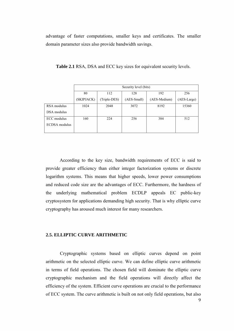
The parameter sizes, generally called the key sizes are listed in Table 2.1.
The listing has been done according to equivalent security levels for RSA, DSA
and ECC as symmetric-key encryption schemes, stated in the table. The
comparison shows that elliptic curve cryptography algorithm uses smaller
parameter sizes than RSA and DSA for the same security levels. That brings the
Page 24
9
advantage of faster computations, smaller keys and certificates. The smaller
domain parameter sizes also provide bandwidth savings.
Table 2.1 RSA, DSA and ECC key sizes for equivalent security levels.
Security level (bits)
80
(SKIPJACK)
112
(Triple-DES)
128
(AES-Small)
192
(AES-Medium)
256
(AES-Large)
RSA modulus
DSA modulus
1024 2048 3072 8192 15360
ECC modulus
ECDSA modulus
160 224 256 384 512
According to the key size, bandwidth requirements of ECC is said to
provide greater efficiency than either integer factorization systems or discrete
logarithm systems. This means that higher speeds, lower power consumptions
and reduced code size are the advantages of ECC. Furthermore, the hardness of
the underlying mathematical problem ECDLP appeals EC public-key
cryptosystem for applications demanding high security. That is why elliptic curve
cryptography has aroused much interest for many researchers.
2.5. ELLIPTIC CURVE ARITHMETIC
Cryptographic systems based on elliptic curves depend on point
arithmetic on the selected elliptic curve. We can define elliptic curve arithmetic
in terms of field operations. The chosen field will dominate the elliptic curve
cryptographic mechanism and the field operations will directly affect the
efficiency of the system. Efficient curve operations are crucial to the performance
of ECC system. The curve arithmetic is built on not only field operations, but also
Page 25
10
on big numbers and modular arithmetic. Elliptic Curve Digital Signature
Algorithm (ECDSA) is an ECC scheme, which needs a hash function and some
modular operations.
Elliptic curve definitions and arithmetic rules will be described in the
following subsections.
2.5.1 Elliptic curve definition
An elliptic curve E over a field K is defined by an equation 2 3 2
1 3 2 4 6:E y a xy a y x a x a x a+ + = + + + (2.1)
Where 1 2 3 4 6, , , ,a a a a a K∈ and 0∆ ≠ , where ∆ is the discriminant of E and is
defined as follows: 2 3 22 8 4 6 2 4 6
22 1 2
4 4 1 3
26 3 6
2 2 28 1 6 2 6 1 3 4 2 3 4
8 27 9
42
4
4
d d d d d d dd a ad a a ad a ad a a a a a a a a a a
∆ = − − − +
= += +
= +
= + − + −
(2.2)
The points of an elliptic curve must satisfy the curve equation and must be in the
same defined field. We can express this in the following way. Let L be any
extension field of K, then the set of L-rational points on E is 2 3 2
1 3 2 4 6( ) {( , ) : 0} { }E L x y L L y a xy a y x a x a x a= ∈ × + + − − − − = ∪ ∞
where ∞ is the point at infinity. The equation (2.1) is called Weierstrass
equation. The condition of 0∆ ≠ ensures that the elliptic curve is smooth. The
smoothness provides that no points on the curve have two distinct tangent lines.
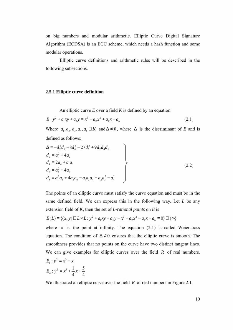
We can give examples for elliptic curves over the field R of real numbers. 2 3
1
2 32
:1 5:4 4
E y x x
E y x x
= −
= + +
We illustrated an elliptic curve over the field R of real numbers in Figure 2.1.
Page 26
11
Figure 2.1 Elliptic curves over R.
We have given the definition of elliptic curves and illustrated an elliptic
curve in the Figure 2.1. In cryptosystems we are going to use the elliptic curves
which have simplified Weierstrass equations. We can divide these simplified
forms into three and let us state the conditions and simplified forms of
Weierstrass equation (2.1).
• If characteristic of field K ≠ 2,3, then with the admissible change of
variables
−+−
−−−→
24124
2163
,36123
),( 3213112
21 aaaaxayaaxyx
the elliptic curve equation is transformed to the following simplified
equation. 2 3y x ax b= + + (2.3)
where ,a b K∈ . The discriminant of this curve is 3 216(4 27 )a b∆ = − + .
• If characteristic of field K =2 and 1 0a ≠ , then with the admissible
change of variables
Page 27
12
+++→ 3
1
234
213
11
321 ,),(
aaaa
yaaa
xayx
the elliptic curve equation transforms the curve equation to 2 3 2y xy x ax b+ = + + (2.4)
where ,a b K∈ and 0≠b . This kind of curve is called non-supersingular
and has b∆ = . If 1 0a = , the admissible change of variables
),(),( 2 yaxyx +→
transforms the curve equation to 2 3 2y cy x ax b+ = + + (2.5)
where , ,a b c K∈ and 0≠c . Such curves are said to be supersingular and
has discriminant 4c∆ = .
• If characteristic of field K =3 and 21 2a a≠ − , the admissible change of
variables
+
+−
+++
−+→ 3
221
31411
221
314 ,),( aaaaaa
axayaaaaa
xyx
transforms the curve equation to 2 3 2y x ax b= + + (2.6)
where ,a b K∈ and 0, ≠ba . This kind of curve is called non-
supersingular and has 3a b∆ = − . If 21 2a a= − , the admissible change of
variables
),(),( 31 axayxyx ++→
transforms the curve equation to 2 3y x ax b= + + (2.7)
where ,a b K∈ and 0≠a . Such curves are said to be supersingular and
has discriminant 3a∆ = − .
The above classifications have different arithmetic rules. We will use the
arithmetic according to the curve which we will design our system on. Now let’s
mention the arithmetic of elliptic curves.
Page 28
13
2.5.2 Group law for elliptic curves
Let E be an elliptic curve and K be the field which our curve is defined
on. Adding two points in E(K) gives a third point in E(K). The addition is
performed according to a rule called chord-tangent-rule. The set of points in E(K)
forms an abelian group with this addition property and the element ∞ which
serves the identity element. Elliptic curve cryptosystems are constructed on
abelian groups.
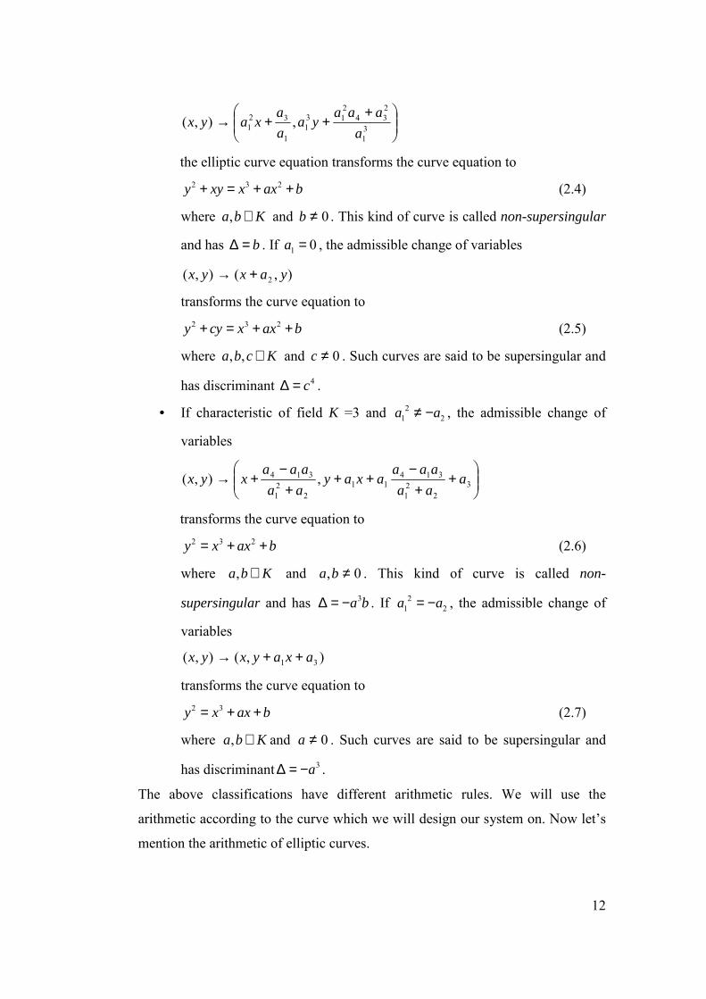
We can explain addition operation geometrically. Let ),( 21 xxP = and
),( 21 xxQ = be two points on an elliptic curve E. The sum of P and Q is defined
as follows. First draw a line through P and Q. This line intersects the curve at a
third point. The reflection of this point about the x-axis is the addition result point
R. This is depicted in Figure 2.2.
Figure 2.2 Geometric addition of elliptic curve points, P+Q=R.
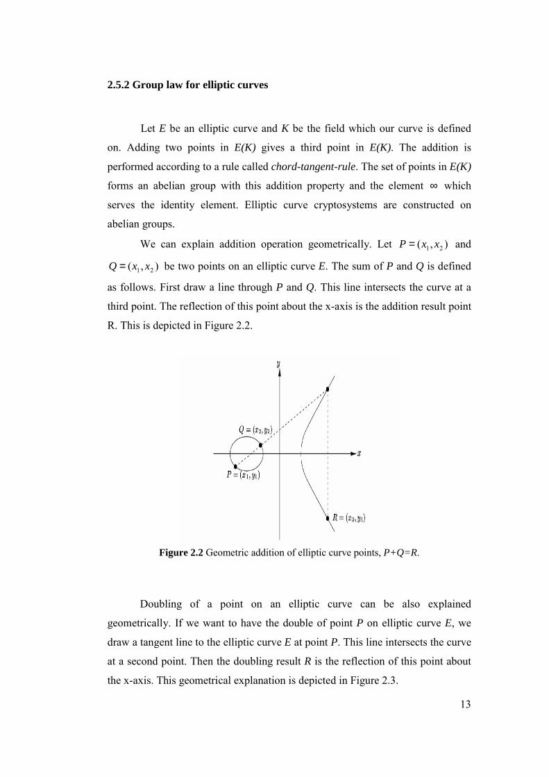
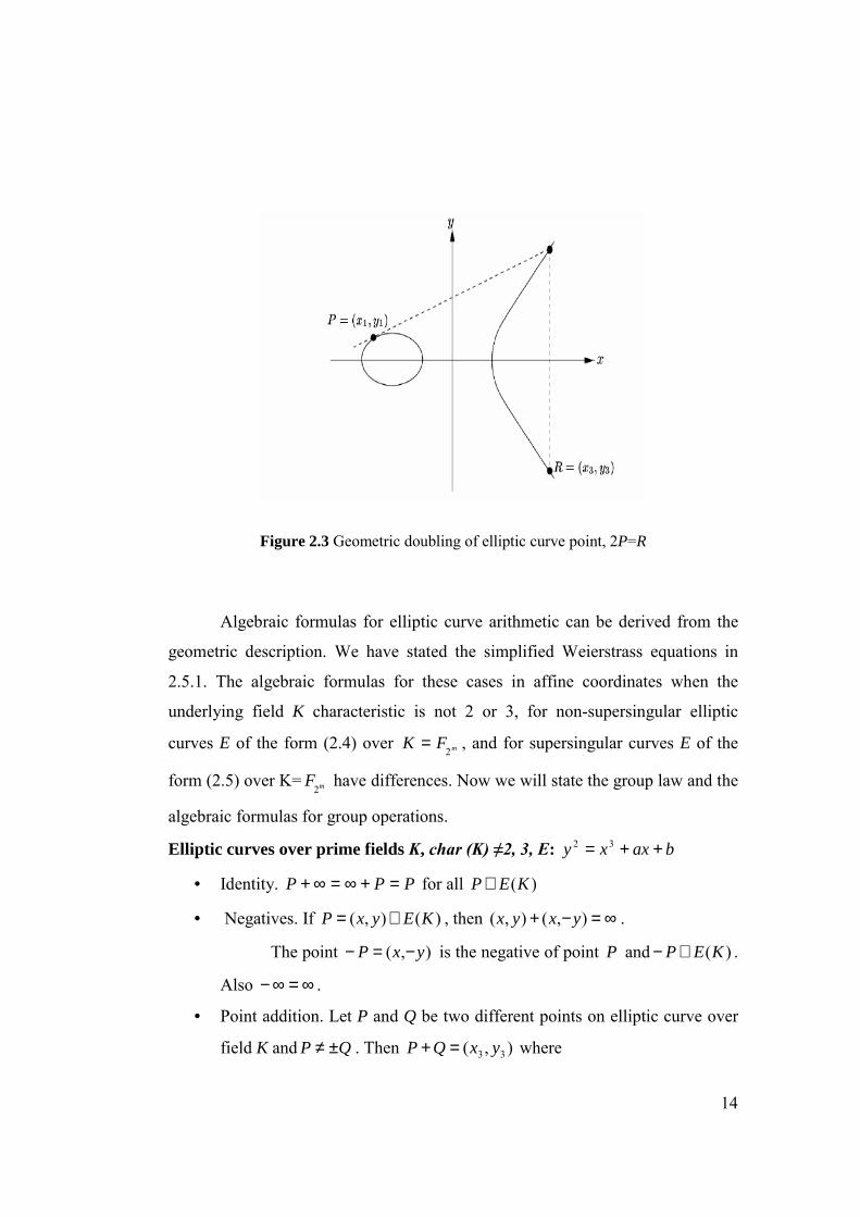
Doubling of a point on an elliptic curve can be also explained
geometrically. If we want to have the double of point P on elliptic curve E, we
draw a tangent line to the elliptic curve E at point P. This line intersects the curve
at a second point. Then the doubling result R is the reflection of this point about
the x-axis. This geometrical explanation is depicted in Figure 2.3.
Page 29
14
Figure 2.3 Geometric doubling of elliptic curve point, 2P=R
Algebraic formulas for elliptic curve arithmetic can be derived from the
geometric description. We have stated the simplified Weierstrass equations in
2.5.1. The algebraic formulas for these cases in affine coordinates when the
underlying field K characteristic is not 2 or 3, for non-supersingular elliptic
curves E of the form (2.4) over mFK 2= , and for supersingular curves E of the
form (2.5) over K=2mF have differences. Now we will state the group law and the
algebraic formulas for group operations.
Elliptic curves over prime fields K, char (K) ≠2, 3, E: baxxy ++= 32
• Identity. PPP =+∞=∞+ for all )(KEP ∈
• Negatives. If )(),( KEyxP ∈= , then ∞=−+ ),(),( yxyx .
The point ),( yxP −=− is the negative of point P and )(KEP ∈− .
Also ∞=∞− .
• Point addition. Let P and Q be two different points on elliptic curve over
field K and QP ±≠ . Then ),( 33 yxQP =+ where
Page 30
15
21
2
12
123 xx
xxyyx −−
−−=
13112
123 )( yxx
xxyyy −−
−−=
• Point doubling. Let )(),( 11 KEyxP ∈= , where PP −≠ . Then
),(2 33 yxP = where
1
2
1
21
3 22
3 xy
axx −
+=
1311
21
3 )(2
3 yxxy
axy −−
+=
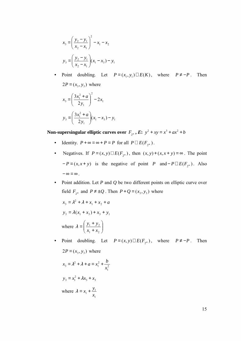
Non-supersingular elliptic curves over 2mF , E: 2 3 2y xy x ax b+ = + +
• Identity. PPP =+∞=∞+ for all )( 2mFEP ∈ .
• Negatives. If )(),( 2mFEyxP ∈= , then ∞=++ ),(),( yxxyx . The point
),( yxxP +=− is the negative of point P and )( 2mFEP ∈− . Also
∞=∞− .
• Point addition. Let P and Q be two different points on elliptic curve over
field mF2 and QP ±≠ . Then ),( 33 yxQP =+ where
axxx ++++= 212
3 λλ
13313 )( yxxxy +++= λ
where
++
=21
21
xxyyλ
• Point doubling. Let )(),( 2mFEyxP ∈= , where PP −≠ . Then
),(2 33 yxP = where
21
21
23 x
bxax +=++= λλ
33213 xxxy ++= λ
where 1
11 x
yx +=λ
Page 31
16
Supersingular elliptic curves over 2mF , E: 2 3 2y cy x ax b+ = + +
• Identity. PPP =+∞=∞+ for all )( 2mFEP ∈ .
• Negatives. If )(),( 2mFEyxP ∈= , then ∞=++ ),(),( cyxyx . The point
),( cyxP +=− is the negative of point P and )( 2mFEP ∈− . Also
∞=∞− .
• Point addition. Let P and Q be two different points on elliptic curve over
field mF2 and QP ±≠ . Then ),( 33 yxQP =+ where
axxx +++= 212
3 λ
cyxxxy ++++= 13313 )(λ
where
++
=21
21
xxyyλ
• Point doubling. Let )(),( 2mFEyxP ∈= , where PP −≠ . Then
),(2 33 yxP = where
221
3
+=c
axx
cyxxc
axy +++
+= 131
21
3 )(
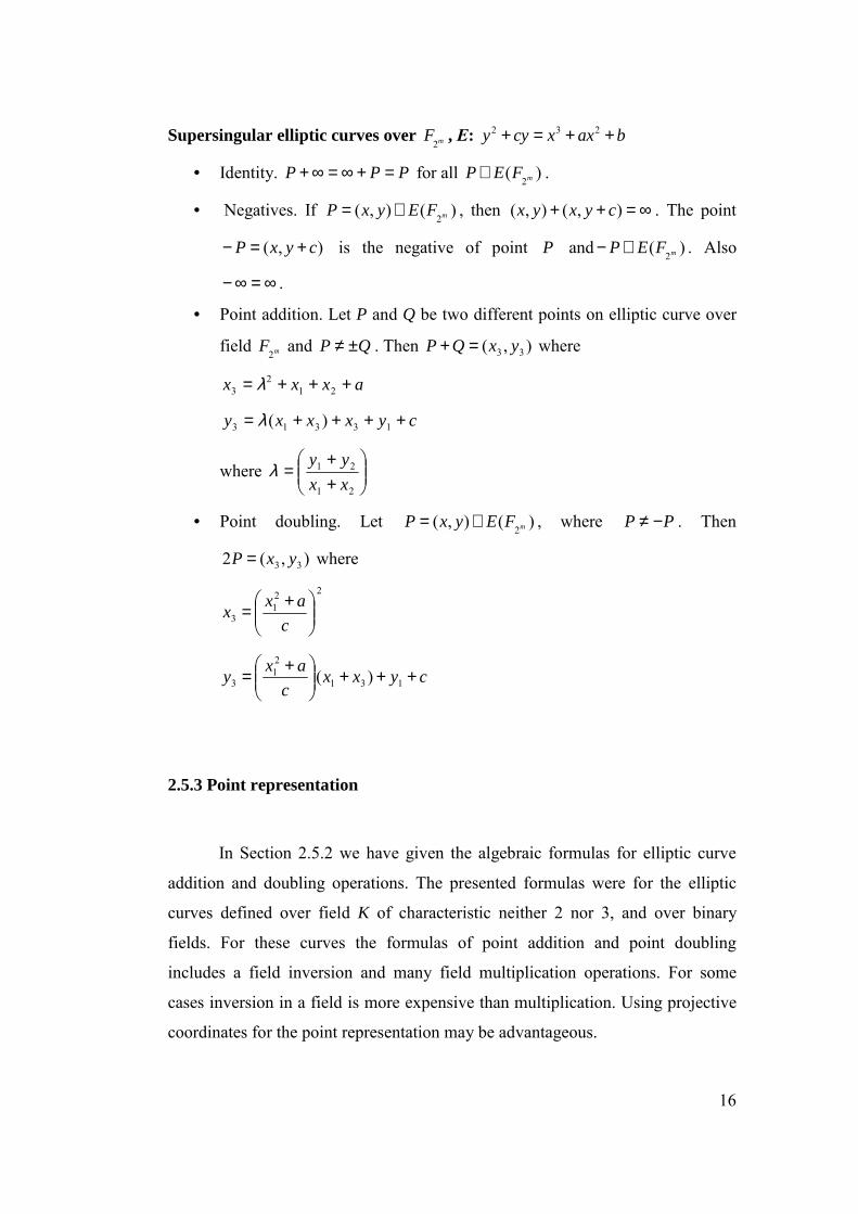
2.5.3 Point representation
In Section 2.5.2 we have given the algebraic formulas for elliptic curve
addition and doubling operations. The presented formulas were for the elliptic
curves defined over field K of characteristic neither 2 nor 3, and over binary
fields. For these curves the formulas of point addition and point doubling
includes a field inversion and many field multiplication operations. For some
cases inversion in a field is more expensive than multiplication. Using projective
coordinates for the point representation may be advantageous.
Page 32
17
We will describe the projective coordinates which will be used to avoid
the expense of field inversion. The benefit of using projective coordinates will be
observed later in the implementation results sections. Let us define a field K, and
positive integers c and d. The definition can be given for an equivalence relation
~ on the set K3 \ {(0,0,0)} of nonzero triples over K by
1 1 1( , , )X Y Z ~ 2 2 2( , , )X Y Z if 1 2cX Xλ= , 1 2
dY Yλ= , 1 2Z Zλ= for some *Kλ ∈ .
We can represent the above expression by another notation as *( : : ) {( , , ) : }c dX Y Z X Y Z Kλ λ λ λ= ∈
where K* represents the set of nonzero elements of the field K.
( : : )X Y Z is called projective point and ( , , )X Y Z is called a representative of
( : : )X Y Z . The set of all projective points is denoted as P(K)
We will use these point representations for our elliptic curve systems.
First Weierstrass equation (2.1) will be transformed. That is performed by
replacing x by / cX Z and y by / dY Z , and clearing denominators. After this
formula transformation, we obtain a projective equation. If ( , , )X Y Z ∈ K3 \
{(0,0,0)} satisfies the projective equation, we can say that the projective point
( : : )X Y Z lies on E [HankMenVan, 2004].
The known projective coordinates for elliptic curve 2 3 2:E y x ax b= + + ,
are as follows [BrHankLopMen, 2001].
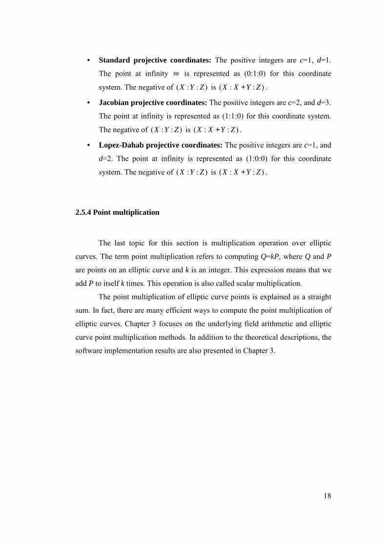
• Standard projective coordinates: The positive integers are c=1, d=1.
The point at infinity ∞ is represented as (0:1:0) for this coordinate
system. The negative of ( : : )X Y Z is ( : : )X Y Z− .
• Jacobian projective coordinates: The positive integers are c=2, and d=3.
The point at infinity is represented as (1:1:0) for this coordinate system.
The negative of ( : : )X Y Z is ( : : )X Y Z− .
• Chudnovsky coordinates: This representation is formed by representing
Jacobian coordinates ( : : )X Y Z as 2 3( : : : : )X Y Z Z Z .
The known projective coordinates for elliptic curve 2 3 2:E y xy x ax b+ = + + ,
are as follows [HankHernMen, 2000].
Page 33
18
• Standard projective coordinates: The positive integers are c=1, d=1.
The point at infinity ∞ is represented as (0:1:0) for this coordinate
system. The negative of ( : : )X Y Z is ( : : )X X Y Z+ .
• Jacobian projective coordinates: The positive integers are c=2, and d=3.
The point at infinity is represented as (1:1:0) for this coordinate system.
The negative of ( : : )X Y Z is ( : : )X X Y Z+ .
• Lopez-Dahab projective coordinates: The positive integers are c=1, and
d=2. The point at infinity is represented as (1:0:0) for this coordinate
system. The negative of ( : : )X Y Z is ( : : )X X Y Z+ .
2.5.4 Point multiplication
The last topic for this section is multiplication operation over elliptic
curves. The term point multiplication refers to computing Q=kP, where Q and P
are points on an elliptic curve and k is an integer. This expression means that we
add P to itself k times. This operation is also called scalar multiplication.
The point multiplication of elliptic curve points is explained as a straight
sum. In fact, there are many efficient ways to compute the point multiplication of
elliptic curves. Chapter 3 focuses on the underlying field arithmetic and elliptic
curve point multiplication methods. In addition to the theoretical descriptions, the
software implementation results are also presented in Chapter 3.
Page 34
19
CHAPTER 3
FIELD ARITHMETIC AND ELLIPTIC CURVE POINT
MULTIPLICATION
Elliptic curve point multiplication is a fundamental issue in elliptic curve
cryptography. That is because it dominates the cryptographic schemes. The
operation is kP, where k is an integer and P is a point on an elliptic curve E
defined over a field. This operation is called point multiplication or scalar
multiplication. In this chapter, the point multiplication techniques are presented
and software implementation results are discussed. Before getting into EC point
multiplication methods and software implementations, we describe the
underlying finite field operations of these algorithms. In Section 3.1, finite field
arithmetic which we have used for our EC software implementations is described
shortly. The timings of field arithmetic operations are presented both for prime
fields and binary fields in Subsection 3.1.3. Section 3.2 covers the theoretical
description of different elliptic curve multiplication methods. The software
implementation of each method has been done in C on a Pentium 4 processor at 3
GHz. Our main concern is the timing results of these implementations. We
present the measured timing performances in Section 3.3.
3.1 FINITE FIELD ARITHMETIC
Since we will deal with the timings of EC point multiplication methods, it
is important to have efficient field arithmetic implementations. We will discuss
implementations in prime fields and binary fields. Efficient methods of addition,
Page 35
20
multiplication, inversion in both prime fields and binary fields are described in
subsections 3.1.1 and 3.1.2 [BrHankLopMen, 2001], [HankHernMen, 2000].
3.1.1 Finite field arithmetic in prime fields
A prime field is formed of integers modulo p, {0,1,2 …p-1} and the
operations of addition and multiplication performed modulo p. The order of the
field is p and represented as pF . The prime number p is the modulus of pF . The
reduction modulo p operation is dividing any integer by p and keeping the
remainder of division for the result. Now let us describe how we perform prime
field arithmetic in software. First we assume that the platform is 32-bit processor.
The elements of pF will be written in binary representation. The number
2logm p= gives the number of bits that we are going to present our field
elements. In our software we can store the prime field elements in
/ 32t m= number of words [Mur, 2003].
Addition and Subtraction
Addition in prime fields is the sum of two integers mod p. The prime
numbers are added word by word and if the sum exceeds p-1, we subtract p from
the sum. After each word addition, we carry a bit for the next word addition and
add it to the next sum. Implementation of modular subtraction is similar to the
implementation of modular addition. But the carry in addition is the borrow in
subtraction. If we have a borrow from the word subtraction, we subtract it from
the next word operation.
Multiplication and squaring
Field multiplication of prime field elements can be performed first
multiplying two integers then reducing the product modulo p. Field squaring can
Page 36
21
be accomplished by first squaring the field element as an integer, then reducing
the result modulo p.
Modular Reduction
The modular reduction is part of field multiplication. In fact it is the
expensive part of multiplication operation. Since we care about the speed of
elliptic curve schemes we should have time efficient modular reduction. Barrett
reduction is generally considered to be the fast reduction technique
[HankMenVan, 2004].
3.1.2 Finite field arithmetic in binary fields
Binary fields are also called characteristic–two finite fields. The elements
of 2mF are often represented with binary polynomials whose coefficients are in
the field 2 {0,1}F = and degree is at most m-1. When programming, we can
represent coefficients as bits of our words. For example, on 32-bit processor
0x20000005 represents the polynomial 29 2 1x x+ + in 312F . A polynomial can be
represented with ( 1) /m w+ words, where polynomial has the degree m and the
word size is w.
Addition
The addition of two polynomials is bitwise xor operations. Let
( 1) /t m w= + where m is the degree of a binary polynomial in a binary field
and w is the word size. The addition of two polynomials whose degree is m needs
t word operations.
Page 37
22
Multiplication
When we multiply two polynomials of degree (m-1) we will obtain a
polynomial of degree (2m-2). Since we are performing finite field operations, this
product should be reduced with respect to an irreducible polynomial ( )f x of
degree m. In order to have fast reduction operations, the irreducible polynomial
with a few terms should be chosen. The modulation operation can be done during
or after the polynomial multiplication.
The basic method for polynomial multiplications is shift-and-add method.
Let a and b be two polynomials and c be their partial product. Shift-and-add
method begins with setting c to 0 if 0 0a = or to b if 0 1a = . Then method goes on
with scanning bits of a. For each bit b is shifted to left by one, and if the bit is 1
we add this shifted b to c [YanShi, 2006].
Some other methods have been also developed for field multiplication.
They are comb algorithms. With these methods faster polynomial multiplications
can be performed. We told that we will store our binary polynomial in t number
of words. The comb methods avoid us testing each bit one by one. Instead we test
each bit 0 of all t words of a. Then the other bits are tested for each word. We can
also test the bits from the most significant bit to the least significant bit. For left
to right comb methods the shifting is done to partial product c. So the input
values remain unchanged. Then we can employ sliding window technique to
reduce shifting. We can scan the bits with a fixed size window and then multiply
more than one bit with b at a time [LopDa, 2000]. Then c is shifted left by the
fixed window size. Since our window size is fixed we can calculate the possible b
products and store them in a table. So the shifting number is reduced by the cost
of storage.
Another point for multiplication of polynomials is polynomial squaring. It
can be performed faster than multiplication operation by inserting 0 bits between
consecutive bits of the polynomial [HankMenVan, 2004].
Page 38
23
Inversion
In Chapter 2, EC operations are described in detail. The definitions tell us
that there exists field inversion in EC addition and doubling operations. The
inverse of an element of 2ma F∈ is the unique element of the same field that
satisfies 1. 1a a− = in 2mF . The classical algorithm for computing multiplicative
inverse is Extended Euclidean Algorithm (EEA) [HankHernMen, 2004]. Since
EEA inversion is stated as the most time efficient inversion we have chosen this
method for our field inversion implementation [YanShi, 2006].
3.1.3 Field arithmetic on Pentium processor
We have implemented both prime field and binary field arithmetic
operations on a Pentium 4 processor at 3 GHz. The field arithmetic routines are
written in C.
In Table 3.1 we have presented the timings of prime field operations
which are addition, subtraction, modular reduction, multiplication, squaring and
inversion. The operations are done in NIST prime fields. It should be noted that
NIST primes provide fast reductions [BrHankLopMen, 2001]. The prime field
arithmetic implementation is based on 16-bit word size. Same calculations are
done in [BrHankLopMen, 2001] but with 32-bit word size and by using hand-
coded assembly code. It is expected that using 32-bit word size and assembly
programming should have better timings. However using Pentium 4 processor
has better timings for addition, subtraction and modular reduction. So we have
obtained noteworthy results for prime field operations. If we want to discuss
about the timing characteristics of prime field operations we can conclude from
the results that inversion and multiplication operation is the expensive field
operations. A noticable point is squaring takes less execution time than
multiplication.
Page 39
24
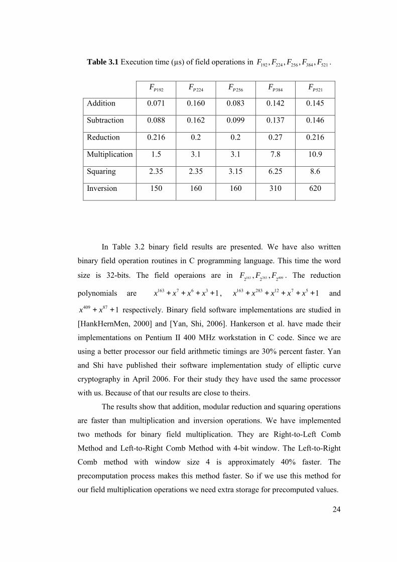
Table 3.1 Execution time (µs) of field operations in 192 224 256 384 521, , , ,F F F F F .
192PF 224PF 256PF 384PF 521PF
Addition 0.071 0.160 0.083 0.142 0.145
Subtraction 0.088 0.162 0.099 0.137 0.146
Reduction 0.216 0.2 0.2 0.27 0.216
Multiplication 1.5 3.1 3.1 7.8 10.9
Squaring 2.35 2.35 3.15 6.25 8.6
Inversion 150 160 160 310 620
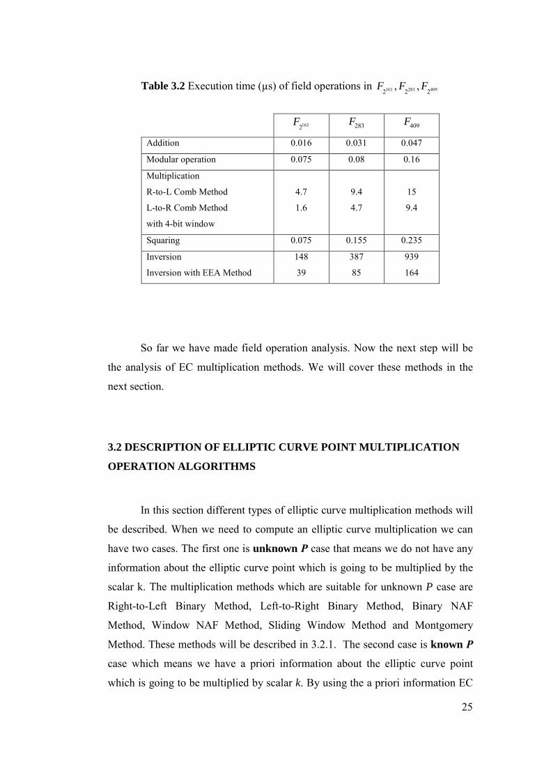
In Table 3.2 binary field results are presented. We have also written
binary field operation routines in C programming language. This time the word
size is 32-bits. The field operaions are in 163 283 4092 2 2, ,F F F . The reduction
polynomials are 163 7 6 3 1x x x x+ + + + , 163 283 12 7 5 1x x x x x+ + + + + and
187409 ++ xx respectively. Binary field software implementations are studied in
[HankHernMen, 2000] and [Yan, Shi, 2006]. Hankerson et al. have made their
implementations on Pentium II 400 MHz workstation in C code. Since we are
using a better processor our field arithmetic timings are 30% percent faster. Yan
and Shi have published their software implementation study of elliptic curve
cryptography in April 2006. For their study they have used the same processor
with us. Because of that our results are close to theirs.
The results show that addition, modular reduction and squaring operations
are faster than multiplication and inversion operations. We have implemented
two methods for binary field multiplication. They are Right-to-Left Comb
Method and Left-to-Right Comb Method with 4-bit window. The Left-to-Right
Comb method with window size 4 is approximately 40% faster. The
precomputation process makes this method faster. So if we use this method for
our field multiplication operations we need extra storage for precomputed values.
Page 40
25
Table 3.2 Execution time (µs) of field operations in 163 283 4092 2 2, ,F F F
1632
F 283F 409F
Addition 0.016 0.031 0.047
Modular operation 0.075 0.08 0.16
Multiplication
R-to-L Comb Method
L-to-R Comb Method
with 4-bit window
4.7
1.6
9.4
4.7
15
9.4
Squaring 0.075 0.155 0.235
Inversion
Inversion with EEA Method
148
39
387
85
939
164
So far we have made field operation analysis. Now the next step will be
the analysis of EC multiplication methods. We will cover these methods in the
next section.
3.2 DESCRIPTION OF ELLIPTIC CURVE POINT MULTIPLICATION
OPERATION ALGORITHMS
In this section different types of elliptic curve multiplication methods will
be described. When we need to compute an elliptic curve multiplication we can
have two cases. The first one is unknown P case that means we do not have any
information about the elliptic curve point which is going to be multiplied by the
scalar k. The multiplication methods which are suitable for unknown P case are
Right-to-Left Binary Method, Left-to-Right Binary Method, Binary NAF
Method, Window NAF Method, Sliding Window Method and Montgomery
Method. These methods will be described in 3.2.1. The second case is known P
case which means we have a priori information about the elliptic curve point
which is going to be multiplied by scalar k. By using the a priori information EC
Page 41
26
point multiplication methods are developed through precomputation steps. The
known elliptic curve point is used to form some data which will be used when EC
point multiplication will be proceeded. So some memory will be required to store
these precomputed data. The known P case methods are Fixed Base Windowing
Method, Fixed Base NAF Windowing Method, Fixed Base Comb Method, and
Fixed Base Comb with two tables Method. We will describe these methods in
3.2.2 step by step.
3.2.1 Point P is unknown
The first algorithms that we are going to introduce you, are the Right-to-
Left Binary and Left-to-Right Binary methods. These methods perform EC point
multiplication operation by processing the scalar k bit by bit from right to left or
left to right. These two methods are the additive versions of repeated-square-and-
multiply methods for exponentiation. The algorithm details are as follows
[HankMenVan, 2004].
Algorithm 3.1 Right to left binary method for point multiplication
INPUT: ),,...,( 011 kkkk t−= )( qFEP ∈
OUTPUT: kP
1. ∞←Q
2. For i from 0 to t-1 do
2.1 If 1=ik then PQQ +←
2.2 PP 2←
3. Return ( Q )
Algorithm 3.2 Left to right binary method for point multiplication
INPUT: ),,...,( 011 kkkk t−= )( qFEP ∈
Page 42
27
OUTPUT: kP
1. ∞←Q
2. For i from t-1 to 0 do
2.1 QQ 2←
2.2 If 1=ik then PQQ +←
3. Return (Q )
Since we will be interested in running time of the multiplication algorithms
we can predict the execution time by looking at the algorithm steps. The scalar k
has t bits and it is expected that t/2 number of ones may be in the binary
representation of k. So the Alg.3.1 and Alg.3.2 may have the running time of
2t A tD+ where A represents elliptic curve point addition and D represents
elliptic curve point doubling times.
The subtraction of points on an elliptic curve is just as efficient as
addition. So a signed digit representation can be used for scalar k. A useful signed
digit representation is the non-adjacent form (NAF). A non-adjacent form (NAF)
of a positive integer k is an expression 1
02l i
iik k−
==∑ . The scalar k has unique
NAF representation denoted as NAF(k) and in this representation, none of the
consecutive bits are nonzero. NAF(k) has fewest nonzero digits than any signed
representation of k. The length of the NAF(k) is almost one more digit more than
the length of the binary representation of k. The attracted point of this
representation is the density of nonzero digits. It is approximately 1/3 [MorOl,
1990]. Now, we will first describe how to represent a binary represented number
in NAF, and then we will substitute this form to scalar k in elliptic curve
multiplication methods.
Computing NAF
INPUT: a positive integer k
OUTPUT: kP
1. 1. ∞←Q
Page 43
28
2. While 1≥k do
2.1 If k is odd then: ii kkkkk −←−← ),4mod(2
2.2 Else 0←ik
2.3 2/kk ← , 1+← ii
3. Return ),,...,,( 0121 kkkk ii −−
By using non-adjacent form Left-to-Right Method can be modified. The
modified multiplication method is as follows.
Algorithm 3.3 Binary NAF method for point multiplication
INPUT: Positive integer k , )( qFEP ∈
OUTPUT: kP
1. Compute ∑−
=
=1
02)(
l
i
iikkNAF
2. ∞←Q
3. For i from l-1 to 0 do
3.1 QQ 2←
3.2 If 1=ik then PQQ +←
3.3 If 1−=ik then PQQ −←
4. Return (Q )
3.2.2 Window Methods
If we have some extra memory in our implementation platform, the
running time of multiplication algorithms can be decreased by using a window
method. In window methods w digits of k are processed at a time so the running
times of algorithms decrease. The notation w means the window width. Before
getting into EC point multiplication methods we want to describe a version of
NAF representation called width-w NAF. In this representation we represent the
Page 44
29
scalar k by odd numbers as 1
02l i
iik k−
==∑ where 12w
ik −< and 1 0lk − ≠ . The
scalar k has a unique width-w NAF representation denoted as NAFw(k). The
average density of nonzero digits of width-w NAF representation is
approximately 1/(w+1) [Sol, 2000]. The computation of width-w NAF
representation is as follows.
Computing width-w NAF of a positive integer
INPUT: Window width w, a positive integer k.
OUTPUT: NAFw (k)
1. 0←i
2. While 1≥k do
2.1. If k is odd then: iw
i kkkkk −←← ,2mod
2.2. Else 0←ik
2.3. 2/kk ← , 1+← ii
3. Return ),,...,,( 0121 kkkk ii −−
If w=2 the NAFw(k) representation will be equal to NAF(k) representation.
We have used NAF representation in Left-to-Right Binary Method for EC point
multiplication. By using width-w NAF representation in this method we can
generalize this EC point multiplication method. That is called Window NAF
method. The steps of this multiplication method are described as follows.
Algorithm 3.4 Window NAF method for point multiplication
INPUT: Positive integer k , )( qFEP ∈
OUTPUT: kP
1. Compute ∑−
=
=1
02)(
l
i
iiw kkNAF
2. Compute iPPi = for }12,...,5,3,1{ 1 −∈ −wi
3. ∞←Q
Page 45
30
4. For i from l-1 to 0 do
4.1 QQ 2←
4.2 If 0≠ik then
If 0>ik then ikPQQ +←
Else ikPQQ −−←
5. Return(Q )
The following method had been developed as an alternative to Window
NAF method. It is another version of computed width-w NAF and using this
representation in Left-to-Right Binary method. In this method we can use a
sliding window on the NAF(k). The window moves left-to-right over the digits
and is placed so that the value in the window is odd. Here we use NAF(k) and
meet the odds as sliding our window from left-to-right. The steps of this
algorithm are stated in detail in Alg.3.5 description [Sol, 2000].
Algorithm 3.5 Sliding window method for point multiplication
INPUT: Positive integer k , )( qFEP ∈
OUTPUT: kP
1. Compute ∑−
=
=1
02)(
l
i
iikkNAF
2. Compute iPPi = for }13/))1(2(2,...,5,3,1{ −−−∈ wwi
3. ∞←Q , 1−← li
4. While 0≥i do
4.1. If 0=ik then 0,1 ←← ut
Else find the largest wt ≤ such that ),...,( 1+−← tii kku is odd.
4.2. QQ t2←
4.3. If 0>u then uPQQ +← ; else if 0<u then uPQQ −−←
4.4. tii −←
5. Return (Q)
Page 46
31
Another algorithm will be described for non-supersingular elliptic curves over
binary fields. This method is due to Lopez and Dahab and it is based on idea of
Montgomery. Using the EC addition formulas we can have the x coordinate of an
EC point addition operation result by using the x-coordinate of the two points and
the x-coordinate of their subtraction result. Let P and Q be the two points that we
want to add. Hence we only need to know the x coordinates of P, Q and P-Q to
determine the x-coordinate of P+Q. Before getting into Montgomery
multiplication method we want to describe addition and doubling computations.
We have stated different point representations in Chapter 2. Here we will
represent x-coordinate of P by X/Z. The coordinates of points 2P and P+Q are as
follows.
Let D = 2.P
4 4
2 2
..
D
D
X X b ZZ X Z
= +
=
and let A = P+Q
2( . . )
. ( . ).( . )A P Q Q P
A A P Q Q P
Z X Z X ZX x Z X Z X Z
= +
= +
We have stated the main operations of Montgomery multiplication
method for elliptic curve points. Below EC point multiplication of Montgomery
Method is described.
Algorithm 3.6 Montgomery point multiplication
INPUT: 1 1 0 2( ,..., , )tk k k k−= with 1 1tk − = , 2
( , ) ( )mP x y E F= ∈
OUTPUT: kP
1. 4 21 1 2 2, 1, ,X x Z X x b Z x← ← ← + ← (P and 2P is computed)
2. For i from t-2 down to 0 do
2.1. If 1ik = then
2
1 1 1 2 2 1 1 1 1 2 24 4 2 2
2 2 2 2 2 2
, ( ) ,, ,
T Z Z X Z X Z X xZ X X TZT X X X bZ Z T Z
← ← + ← +
← ← + ←
Page 47
32
2.2. else
2
2 2 1 2 2 1 2 2 1 2 14 4 2 2
1 1 1 1 1 1
, ( ) ,, ,
T Z Z X Z X Z X xZ X X TZT X X X bZ Z T Z
← ← + ← +
← ← + ←
3. Convert the results to affine coordinates 3 3( , )x y .
4. Return 3 3( , )x y .
3.2.3 Point P is known
We may have some cases that we know the point P a priori. With this
information we can precompute some data based on P and store it. This can be
done when there exists enough memory. The precomputed data will accelarate
our point multiplication operation kP. In this section we will describe the EC
point multiplication methods based on known point P.
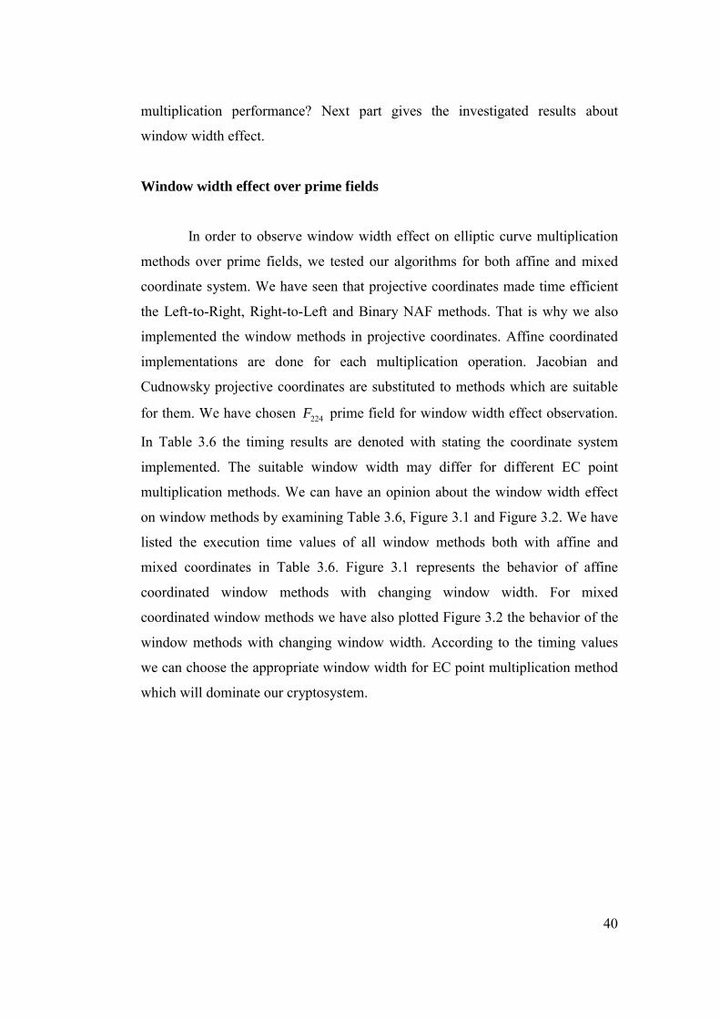
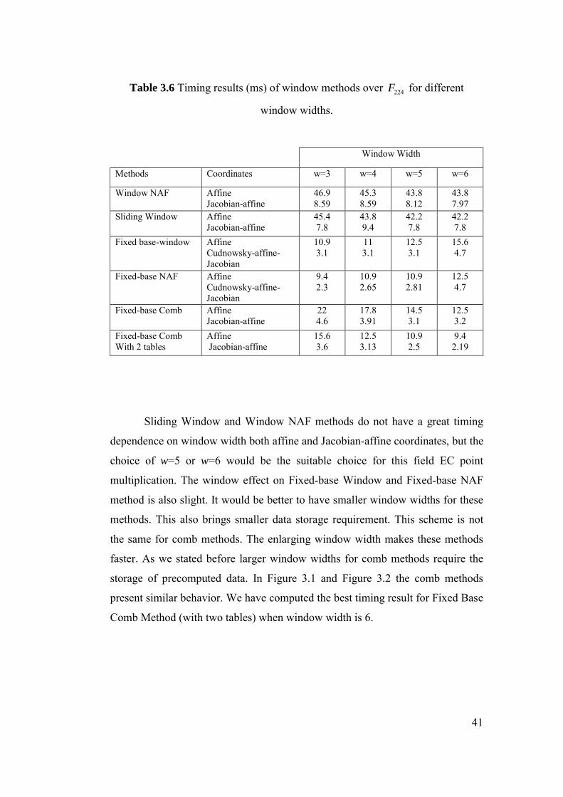
The first method will be the Fixed-base Windowing Method. For this
method we will precompute every multiple 2i P and base-2w representation of k
will be used.
Algorithm 3.7 Fixed-base windowing method for point multiplication
INPUT: Window width w, wtd /= , wKKKk d 2011 ),,...,( −= , )( qFEP ∈
OUTPUT: kP
1. Precomputation: Compute 10,2 −≤≤= diPP wii
2. ∞←∞← BA ,
3. For j from 12 −w down to 1 do
3.1. For each i for which jKi = do: iPBB +←
3.2. BAA +←
4. Return (A).
Page 48
33
The execution time of the Fixed-base windowing Method is expected as
(2w+d-3)A where A is EC point addition execution time. We can modify this
method by using NAF representation instead of binary representation for k. The
modified version of this method is described as follows.
Algorithm 3.8 Fixed-base NAF windowing method for point multiplication
INPUT: Window width w, positive integer k , )( qFEP ∈
OUTPUT: kP
1. Precomputation: Compute wtiPP wii /)1(0,2 +≤≤=
2. Compute ∑−
=
=1
02)(
l
i
iikkNAF
3. wld /←
5. By padding NAF (k) on the left with 0s if necessary, write
011011 ||||...||),,...,( KKKkkk dl −− = where each iK is a }1,0{ ± string of length
d.
6. If w is even then 3/)22( 1 −← +wI ; else 3/)12( 1 −← +wI
7. ∞←∞← BA ,
8. For j from I down to 1 do
8.1. For each i for which jKi = do: iPBB +←
8.2. For each I for which jKi −= do iPBB −←
8.3. BAA +←
9. Return(A)
Another known point EC point multiplication style is fixed-base combing. In
comb method we manipulate with scalar k again. We will form a matrix from the
bits of k. The first thing is compute a parameter /d t w= where t is the bit
number of k. We will pad on the left of k with d. (w-t) number of zeros and divide
the padded k into w bit strings. These strings will form the rows of our matrix and
has the d number of bits. So we have a w d× matrix. For precomputation we will
Page 49
34
compute 1 1 0[ ,..., , ]wa a a P− for all possible bit strings and store the results. This
method is described in detail in Alg.3.9.
Algorithm 3.9 Fixed-base comb method for point multiplication
INPUT: Window width w, wtd /= , wkkkk t 2011 ),,...,( −= , )( qFEP ∈
OUTPUT: kP
1. Precomputation: Compute [ ]Paaaw 011 ,,...,− for all bit strings ),,...,( 011 aaaw−
of length w.
2. By padding k on the left with 0s if necessary, 011 ||||...|| KKKk w−= where
each jK is a bit string of length d. Let jiK denote the ith bit of jK .
3. ∞←Q
4. For i from 1−d down to 0 do
4.1. QQ 2←
4.2. [ ]PKKKQQ iiwi
011 ,,...,−+←
5. Return(A).
We can accelerate this method if we can tolerate some additional storage. We
can use a second table of precomputations. So we can call fewer EC doubling
operations. This method is described in Alg.3.10.
Algorithm 3.10 Fixed-base comb method (with two tables) for point
multiplication
INPUT: Window width w, wtd /= , 2/de = , wkkkk t 2011 ),,...,( −= ,
)( qFEP ∈
OUTPUT: kP
1. Precomputation: Compute [ ]Paaaw 011 ,,...,− and [ ]Paaawe
011 ,,...,2 − for all bit
strings ),,...,( 011 aaaw− of length w.
Page 50
35
2. By padding k on the left with 0s if necessary, 011 ||||...|| KKKk w−= where
each jK is a bit string of length d. Let jiK denote the ith bit of jK .
3. ∞←Q
4. For i from 1−e down to 0 do
4.1 QQ 2←
4.2 [ ] [ ]PKKKPKKKQQ eieiw
eie
iiwi
011011 ,,...,2,,..., ++−
+− ++←
5. Return (Q).
3.3 PERFORMANCE COMPARISON OF ELLIPTIC CURVE POINT
MULTIPLICATION METHODS
We have stated the theoretical descriptions of elliptic curve multiplication
methods. In this section we are going to examine these methods in real life.
Elliptic curve point multiplication operation which is going to be handled in a
cryptographic system should be implemented in a most appropriate and desired
way. That is why the comparison work will be helpful in choosing the appropriate
method to substitute in a real system. Our main aim is to find out the efficient and
accelerated EC point multiplication method. We have chosen firstly to work on
different fields with the idea of field operation speeds variety. Prime fields and
binary fields became our computation area. In part 3.2.1 the EC point
multiplication methods are examined over prime fields. The following part 3.2.2
will cover the EC point multiplication methods over binary fields. We will try to
go further by including point representation schemes and window width effect for
each field.
3.3.1 EC point multiplication over Prime Fields
Point multiplication over prime fields is done by field operations. First of
all we choose our field for our system. In February 2000, FIPS 186-1 was revised
Page 51
36
by NIST to include the elliptic curve digital signature algorithm (ECDSA) as
specified in ANSI X9.62 [ANSI, 1999] with further recommendations for the
selection of underlying finite fields and elliptic curves; the revised standard is
called FIPS 186-2 [NIST, 2000] [BrHankLopMen, 2001].
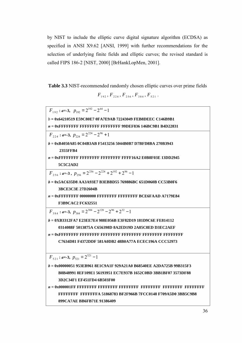
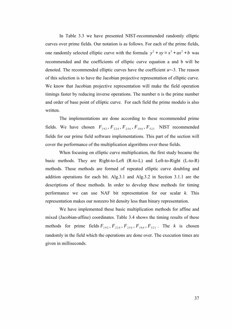
Table 3.3 NIST-recommended randomly chosen elliptic curves over prime fields
1 9 2 2 2 4 2 5 6 3 8 4 5 2 1, , , ,F F F F F .
1 9 2F : a=-3, 122 64192192 −−=p
b = 0x64210519 E59C80E7 0FA7E9AB 72243049 FEB8DEEC C146B9B1
n = 0xFFFFFFFF FFFFFFFF FFFFFFFF 99DEF836 146BC9B1 B4D22831
2 2 4F : a=-3, 122 96224224 +−=p
b = 0xB4050A85 0C04B3AB F5413256 5044B0B7 D7BFD8BA 270B3943
2355FFB4
n = 0xFFFFFFFF FFFFFFFF FFFFFFFF FFFF16A2 E0B8F03E 13DD2945
5C5C2AD2
2 5 6F : a=-3 , 12222 96192224256256 −++−=p
b = 0x5AC635D8 AA3A93E7 B3EBBD55 769886BC 651D060B CC53B0F6
3BCE3C3E 27D2604B
n = 0xFFFFFFFF 00000000 FFFFFFFF FFFFFFFF BCE6FAAD A7179E84
F3B9CAC2 FC632551
3 8 4F : a=-3, 12222 3296128384384 −+−−=p
b = 0XB3312FA7 E23EE7E4 988E056B E3F82D19 181D9C6E FE814112
0314088F 5013875A C656398D 8A2ED19D 2A85C8ED D3EC2AEF
n = 0xFFFFFFFF FFFFFFFF FFFFFFFF FFFFFFFF FFFFFFFF FFFFFFFF
C7634D81 F4372DDF 581A0DB2 48B0A77A ECEC196A CCC52973
5 2 1F : a=-3, 12521521 −=p
b = 0x00000051 953EB961 8E1C9A1F 929A21A0 B68540EE A2DA725B 99B315F3
B8B48991 8EF109E1 56193951 EC7E937B 1652C0BD 3BB1BF07 3573DF88
3D2C34F1 EF451FD4 6B503F00
n = 0x000001FF FFFFFFFF FFFFFFFF FFFFFFFF FFFFFFFF FFFFFFFF FFFFFFFF
FFFFFFFF FFFFFFFA 51868783 BF2F966B 7FCC0148 F709A5D0 3BB5C9B8
899CA7AE BB6FB71E 91386409
Page 52
37
In Table 3.3 we have presented NIST-recommended randomly elliptic
curves over prime fields. Our notation is as follows. For each of the prime fields,
one randomly selected elliptic curve with the formula baxxxyy ++=+ 232 was
recommended and the coefficients of elliptic curve equation a and b will be
denoted. The recommended elliptic curves have the coefficient a=-3. The reason
of this selection is to have the Jacobian projective representation of elliptic curve.
We know that Jacobian projective representation will make the field operation
timings faster by reducing inverse operations. The number n is the prime number
and order of base point of elliptic curve. For each field the prime modulo is also
written.
The implementations are done according to these recommended prime
fields. We have chosen 1 9 2 2 2 4 2 5 6 3 8 4 5 2 1, , , ,F F F F F NIST recommended
fields for our prime field software implementations. This part of the section will
cover the performance of the multiplication algorithms over these fields.
When focusing on elliptic curve multiplication, the first study became the
basic methods. They are Right-to-Left (R-to-L) and Left-to-Right (L-to-R)
methods. These methods are formed of repeated elliptic curve doubling and
addition operations for each bit. Alg.3.1 and Alg.3.2 in Section 3.1.1 are the
descriptions of these methods. In order to develop these methods for timing
performance we can use NAF bit representation for our scalar k. This
representation makes our nonzero bit density less than binary representation.
We have implemented these basic multiplication methods for affine and
mixed (Jacobian-affine) coordinates. Table 3.4 shows the timing results of these
methods for prime fields 1 9 2 2 2 4 2 5 6 3 8 4 5 2 1, , , ,F F F F F . The k is chosen
randomly in the field which the operations are done over. The execution times are
given in milliseconds.
Page 53
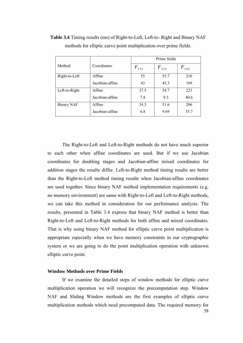
38
Table 3.4 Timing results (ms) of Right-to-Left, Left-to- Right and Binary NAF
methods for elliptic curve point multiplication over prime fields.
Prime fields
Method
Coordinates 1 9 2F 2 2 4F 3 8 4F
Right-to-Left Affine
Jacobian-affine
55
43
55.7
45.3
216
169
Left-to-Right Affine
Jacobian-affine
37.5
7.8
54.7
9.3
223
40.6
Binary NAF Affine
Jacobian-affine
34.3
6.8
51.6
9.69
206
35.7
The Right-to-Left and Left-to-Right methods do not have much superior
to each other when affine coordinates are used. But if we use Jacobian
coordinates for doubling stages and Jacobian-affine mixed coordinates for
addition stages the results differ. Left-to-Right method timing results are better
than the Right-to-Left method timing results when Jacobian-affine coordinates
are used together. Since binary NAF method implementation requirements (e.g.
no memory environment) are same with Right-to-Left and Left-to-Right methods,
we can take this method in consideration for our performance analysis. The
results, presented in Table 3.4 express that binary NAF method is better than
Right-to-Left and Left-to-Right methods for both affine and mixed coordinates.
That is why using binary NAF method for elliptic curve point multiplication is
appropriate especially when we have memory constraints in our cryptographic
system or we are going to do the point multiplication operation with unknown
elliptic curve point.
Window Methods over Prime Fields
If we examine the detailed steps of window methods for elliptic curve
multiplication operation we will recognize the precomputation step. Window
NAF and Sliding Window methods are the first examples of elliptic curve
multiplication methods which need precomputed data. The required memory for
Page 54
39
implementation of these kinds of methods is the one of the issues that we should
investigate. If memory is a constraint for a cryptographic system the designer
should choose the most suitable method. If memory is not a constraint in a
cryptographic system we can prefer fixed base methods. Fixed base methods need
more data storage with better timing results for EC point multiplication operation.
In order to see the memory usage for these methods we have presented storage
requirements. In Table 3.5, the storage requirements are stated for different
window widths. The window width is shown by the letter w.
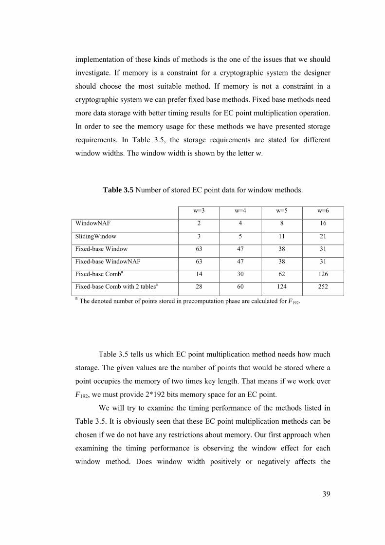
Table 3.5 Number of stored EC point data for window methods.
w=3 w=4 w=5 w=6
WindowNAF 2 4 8 16
SlidingWindow 3 5 11 21
Fixed-base Window 63 47 38 31
Fixed-base WindowNAF 63 47 38 31
Fixed-base Comba 14 30 62 126
Fixed-base Comb with 2 tablesa 28 60 124 252
a The denoted number of points stored in precomputation phase are calculated for F192.
Table 3.5 tells us which EC point multiplication method needs how much
storage. The given values are the number of points that would be stored where a
point occupies the memory of two times key length. That means if we work over
F192, we must provide 2*192 bits memory space for an EC point.
We will try to examine the timing performance of the methods listed in
Table 3.5. It is obviously seen that these EC point multiplication methods can be
chosen if we do not have any restrictions about memory. Our first approach when
examining the timing performance is observing the window effect for each
window method. Does window width positively or negatively affects the
Page 55
40
multiplication performance? Next part gives the investigated results about
window width effect.
Window width effect over prime fields
In order to observe window width effect on elliptic curve multiplication
methods over prime fields, we tested our algorithms for both affine and mixed
coordinate system. We have seen that projective coordinates made time efficient
the Left-to-Right, Right-to-Left and Binary NAF methods. That is why we also
implemented the window methods in projective coordinates. Affine coordinated
implementations are done for each multiplication operation. Jacobian and
Cudnowsky projective coordinates are substituted to methods which are suitable
for them. We have chosen 224F prime field for window width effect observation.
In Table 3.6 the timing results are denoted with stating the coordinate system
implemented. The suitable window width may differ for different EC point
multiplication methods. We can have an opinion about the window width effect
on window methods by examining Table 3.6, Figure 3.1 and Figure 3.2. We have
listed the execution time values of all window methods both with affine and
mixed coordinates in Table 3.6. Figure 3.1 represents the behavior of affine
coordinated window methods with changing window width. For mixed
coordinated window methods we have also plotted Figure 3.2 the behavior of the
window methods with changing window width. According to the timing values
we can choose the appropriate window width for EC point multiplication method
which will dominate our cryptosystem.
Page 56
41
Table 3.6 Timing results (ms) of window methods over 224F for different
window widths.
Window Width
Methods Coordinates w=3 w=4 w=5 w=6
Window NAF Affine Jacobian-affine
46.9 8.59
45.3 8.59
43.8 8.12
43.8 7.97
Sliding Window Affine Jacobian-affine
45.4 7.8
43.8 9.4
42.2 7.8
42.2 7.8
Fixed base-window Affine Cudnowsky-affine-Jacobian
10.9 3.1
11 3.1
12.5 3.1
15.6 4.7
Fixed-base NAF Affine
Cudnowsky-affine-Jacobian
9.4 2.3
10.9 2.65
10.9 2.81
12.5 4.7
Fixed-base Comb Affine
Jacobian-affine 22 4.6
17.8 3.91
14.5 3.1
12.5 3.2
Fixed-base Comb With 2 tables
Affine Jacobian-affine
15.6 3.6
12.5 3.13
10.9 2.5
9.4 2.19
Sliding Window and Window NAF methods do not have a great timing
dependence on window width both affine and Jacobian-affine coordinates, but the
choice of w=5 or w=6 would be the suitable choice for this field EC point
multiplication. The window effect on Fixed-base Window and Fixed-base NAF
method is also slight. It would be better to have smaller window widths for these
methods. This also brings smaller data storage requirement. This scheme is not
the same for comb methods. The enlarging window width makes these methods
faster. As we stated before larger window widths for comb methods require the
storage of precomputed data. In Figure 3.1 and Figure 3.2 the comb methods
present similar behavior. We have computed the best timing result for Fixed Base
Comb Method (with two tables) when window width is 6.
Page 57
42
WNAFSW
FW
FNAF
FC
FCw2T
0
5
10
15
20
25
30
35
40
45
50
3 4 5 6Window width
Exec
utio
n tim
e w
ith a
ffin
e co
ordi
nate
s (m
s)
Figure 3.1 Timings of EC point multiplication window methods at affine coordinates
versus window width.
WNAF
SW
FBW
FBNAF
FC
FBw2T
0
1
2
3
4
5
6
7
8
9
10
3 4 5 6Window width
Exec
utio
n tim
e w
ith a
ffin
e co
ordi
nate
s (m
s)
Figure 3.2 Timings of EC point multiplication window methods at mixed coordinates
versus window width.
Page 58
43
General Look to Execution Times of Elliptic Curve Multiplication Methods
over Prime Fields
In this part of the chapter we will talk about the timing results of the
elliptic curve multiplication methods over prime fields generally. In a
cryptographic system design which we are going to use elliptic curve
cryptography we should choose the most suitable multiplication operation for our
system. That is because of the big role of elliptic curve multiplication operation
for ECDSA (Elliptic Curve Digital Signature Algorithm) or elliptic curve key
exchange algorithms. We have chosen the best timing results for different
platforms. Table 3.7 represents the timing results of these chosen algorithms.
Since using projective coordinates in EC point multiplications eliminates field
inversion operation we prefer using mixed coordinates instead of using only
affine coordinates.
After the evaluation of elliptic curve multiplication operation over prime
fields, we will study binary field case. The next section will cover the same path
of evaluation of this section.
Table 3.7 Timings (ms) of common multiplication methods for different prime
fields.
Multiplication
Method
Memory
usage 192F 224F 256F 384F 521F
Left-to-Right
NO 7.8 9.3 15.6 40.6 78
Window NAF
YES 6.09b
8.12 c
11.7 c
29.2 d
57.35 d
Fixed-base
window
YES 1.5 a
3.1 a
3.6 c
17.2 c
17.2 b
Fixed-base Comb
with 2 Tabled YES 1.41
2.19
3.12
7.5 15.4
aThe window width is 3, bThe window width is 4, cThe window width is 5, dThe window width is
6.
Page 59
44
3.2.2 EC point multiplication over Binary Fields
Point multiplication over binary fields is done by bit operations. We know
that multiplication operation over elliptic curves is formed of several addition
operations. In binary fields, addition of field elements is performed bitwise xor-
ing the vector representations. The field mF2 can be viewed as a vector space of
dimension m over 2F . There exists a set of m elements }{ 110 ,...,, −mααα in
mF2 such that each mF2∈α can be uniquely written in the form
∑−
=
=1
0,
m
ii ia αα where }1,0{∈ia
We can represent alpha as the binary vector ),...,,( 110 −maaa .
Firstly, we choose our binary field for our system. In February 2000, FIPS
186-1 was revised by NIST to include the elliptic curve digital signature
algorithm (ECDSA) as specified in ANSI X9.62 [ANSI, 1999] with further
recommendations for the selection of underlying finite fields and elliptic curves;
the revised standard is called FIPS 186-2 [NIST, 2000]. There are 5
recommended binary fields. They are 571409283233163 22222 ,,,, FFFFF . Our
implementations are done over these recommended binary fields. In this part of
the chapter, we are going to examine the EC point multiplication algorithms and
their performances over binary fields.
We have chosen the 571409283233163 22222 ,,,, FFFFF NIST recommended fields for
our calculations. Table 3.5 gives the parameters of these recommended fields.
The implementations in this study are performed according to these parameters.
The following notation is used. The elements of mF2 are represented using a
polynomial basis representation with reduction polynomial, f(x). An elliptic curve
E over mF2 is specified by the coefficients mFba 2, ∈ of its equation
baxxxyy ++=+ 232 . The number of points on E defined over mF2 is nh , where
n is prime, and h is the cofactor.
Page 60
45
Table 3.8 NIST-recommended elliptic curves over 163 233 409283 5712 2 2, , , ,F F F F F .
1632F : a=1, 163 7 6 3( ) 1f z z z z z= + + + +
b = 0x00000002 0A601907 B8C953CA 1481EB10 512F7874 4A3205FD
n = 0x00000004 00000000 000000000 000292FE 77EC0C12 A4234C33
2332F : a=1, 233 74( ) 1f z z z= + +
b = 0x00000066 647EDE6C 332C7F8C 0923BB58 213B333B 20E9CE42
81FE115F 7D8F90AD
n = 0x00000100 00000000 00000000 00000000 0013E974 E72F8A69
22031D26 03CFE0D7
283F : a=1 , 283 12 7 5( ) 1f z z z z z= + + + +
b = 0x027B680A C8B8596D A5A4AF8A 19A0303F CA97FD76 45309FA2
A581485A F6263E1 3B79A2F5
n = 0x03FFFFFF FFFFFFFF FFFFFFFF FFFFFFFF FFFFEF90 399660FC
938A9016 5B042A7C EFADB307
4092F : a=1 , 409 87( ) 1f z z z= + +
b = 0x0021A5C2 C8EE9FEB 5C4B9A75 3B7B476B 7FD6422E F1F3DD67
4761FA99 D6AC27C8 A9A197B2 72822F6C D57A55AA 4550AE31
7B13545F
n = 0x01000000 00000000 00000000 00000000 00000000 00000000
000001E2 5FA47C3C 9E052F83 8164CD37 D9A21173
571F : a=1 , 571 10 5 2( ) 1f z z z z z= + + + +
b = 0x02F40E7E 2221F295 DE297117 B7F3D62F 5C6A97FF CB8CEFF1 CD6BA8CE
4A9A18AD 84FFABBD 8EFA5933 2BE7AD67 56A66E29 4AFD185A 78FF12AA
520E4DE7 39BACA0C 7FFEFF7F 2955727A
n = 0x03FFFFFF FFFFFFFF FFFFFFFF FFFFFFFF FFFFFFFF FFFFFFFF FFFFFFFF
FFFFFFFF FFFFFFFF E661CE18 FF559873 08059B18 6823851E C7DD9CA1
161DE93D 5174D66E 8382E9BB 2FE84E47
As we did for prime fields we have studied elliptic curve multiplication
implementations for binary fields. All the methods that we have described in
section 3.1 are written in C programming language. We begin with the basic EC
point multiplication methods which are Right-to-Left, Left-to-Right Binary and
Page 61
46
Binary NAF, Montgomery. Since we can use these methods for platforms both
with constraint and adequate memory, we call these methods basic methods.
These EC point multiplication methods are especially for memoryless systems
and for the case of unknown curve point. Both affine and projective coordinates
are substituted for the methods. The Montgomery Method uses projective
coordinates. The timings are affected by the coordinate choice. We stated our
execution time results in Table 3.9 below.
Table 3.9 Timing results (ms) of Right to Left (RTL), Left to Right (LTR) and
Binary NAF methods for elliptic curve point multiplication over binary fields.
Binary fields
Method
Coordinates 1632
F 2832F 4092
F
RTL
Affine
Projective
12.5
7.8
42
26
109
68
LTR
Affine
Projective
12
4.7
40.6
10.9
112
31
Binary NAF
Affine
Projective
11
3.1
37
10.9
96
23
Montgomery Projective 3.1 7.8 21.8
As expected, the performance decreases with the increasing field size.
That refers to the key size in elliptic curve cryptography that will determine the
cryptographic performance. In Table 3.6, it is obviously concluded that
coordinate choice has a great effect on the timings. Using projective coordinates
instead of affine coordinates gives at least 50% better results. When we use affine
coordinates for these basic multiplication methods, the results do not present any
superiority among different methods. Because of that, we can choose any of these
methods for affine coordinated software. But if we can use projective
coordinates, the methods will show better timing performance. Between the
Page 62
47
projective coordinated implementation results of these methods, Montgomery
method should be the most appropriate choice.
As described in the previous sections, there is a concept of window width
that provides faster EC point multiplication methods. Now, we will study this
scheme and try to find a performance relation with the chosen window width in
binary fields.
Window width effect over binary fields
In this part the described window methods for elliptic curve
multiplications will be studied over binary fields. The window methods are
Window NAF, Sliding window, Fixed Base Window , Fixed Base NAF, Fixed
Base Comb, Fixed Base Comb (with two tables) methods. We have implemented
each of these methods with different window widths. The results are presented in
Table 3.7. The multiplications are done over 1632F field by using both affine and
projective coordinates. From the results we can conclude that window width does
not have a noticeable effect on multiplication durations when we use projective
coordinates. If we use affine coordinates, w=4 for Fixed Base Window method,
w=5 for Fixed Base NAF method, w=6 for Fixed Base Comb methods are the
good choices for window widths to have fast elliptic curve multiplication
operations. Widening window width affects comb methods in a good way that
their execution times decrease.
Page 63
48
Table 3.10 Timing results (ms) of window methods over 1632F for different
window widths.
Window Width
Methods Coordinates w=3 w=4 w=5 w=6
Window NAF Affine
Projective
9.4
3.1
9.4
1.5
7.8
3.1
9.3
1.6
Sliding Window Affine
Projective
9.4
3.1
9.4
3.1
7.8
1.6
9.4
1.5
Fixed base-window Affine
Projective
3.1
1.6
1.6
1.6
3.2
3.1
4.7
1.6
Fixed-base NAF Affine
Projective
2.35
1.57
2.3
1.7
2.5
2.3
3.44
3.4
Fixed-base Comb Affine
Projective
4.7
1.6
3.2
1.5
3.2
1.6
1.6
1.6
Fixed-base Comb
(with 2 tables)
Affine
Projective
3.1
1.5
3.1
1.5
1.5
1.5
1.6
1.5
After investigating elliptic curve multiplication over binary fields we
conclude that using projective coordinates make our multiplication performance
better. So using projective coordinates instead of affine coordinates may be our
first choice for our cryptographic system design. According to the memory
constraints of the system it is better to use Montgomery method for memoryless
systems. If we have enough memory for the precomputations we can use Fixed-
base window or Fixed-base Comb methods. We have chosen the appropriate
window widths for speed of the window methods
General Look to Execution Times of Elliptic Curve Multiplication Methods
over Binary Fields
Binary field elliptic curve multiplications have been implemented for
different binary fields, multiplication methods, and different multiplication
Page 64
49
method parameters (e.g. window width, coordinate system). A general look to our
results will be figured and detailed in the following table. We have chosen the
fast results for different possibility of conditions. If we want to design a
cryptographic system based on elliptic curve cryptography, we can choose the
appropriate EC point multiplication method by examining this table. Which
method would be suitable for a design? To answer of this question we should
check out the conditions that we have. For example if we do not have much
memory to store some data, our choice would be a multiplication method without
using any precomputation. The implementation complexity should be another
choice and depends on the software designer’s preference. There is also a case
that we cannot precompute any data before multiplication operation proceeds.
This is multiplication of unknown EC point. In order to draw a conclusion about
the choice of multiplication method we should consider memory, software
platform meaning the processor that EC algorithms will run over, and the case
which we meet an unknown point.
Table 3.11 Timings (ms) of common EC point multiplication methods.
Method Memory
requirement 1632
F 2832F 4092
F
Left-to-Right NO 12 10.9 31
Sliding Window YES 1.6 7.4 18
Montgomery NO 3.1 7.8 21.8
Fixed-base Window YES 1.6 4.7 12.5
FBComb NO 1.6 3.2 7.8
Page 65
50
3.4 COMMENTS ON ELLIPTIC CURVE MULTIPLICATION
IMPLEMENTATIONS
The efficiency of the underlying finite field operations supply the
dominant performance of all elliptic curve operation schemes. If we ask the
question of which field is the best choice, there can not be a single correct
answer, since it depends on the constraints such as the processor type or memory
requirements. In this study we have worked on Pentium 4 processor at 3 GHz and
our code size is 200 KB for prime field implementations and 160 KB for binary
field implementations .
Our main study is presented as the analysis of elliptic curve multiplication
methods in Section 3.2 and in Section 3.3. We first approach the analysis over
different fields. For both prime and binary fields, we have examined the
multiplication method properties and their behaviours against the changing
crucial parameters. The operations over binary fields are faster and easier to
implement than the operations over prime fields of approximately the same size.
Our timing results also show better performance of binary fields on PC.
The path of investigation of multiplication methods is routed through the
known point and unknown point cases. Especially known point multiplications
are significantly faster than the random unknown point multiplications. As we
have stated many times, the aid of precomputation step supplies faster
multiplication operations.
Window width effect was one of our study themes for timing analysis of
the window multiplication methods. We have seen that for fixed-base methods,
wider window widths affect the performance of multiplication operation
positively.
We have seen that coordinate choice has a great effect on the timing
performance of EC point multiplication operations. Using projective coordinates
such as Jacobian or Cudnowsky for prime fields, and standart projective
coordinates for binary fields make our multiplication performances faster. In
Section 3.1, our field arithmetric software implementation study shows that the
most expensive field operation is field inversion. Since projective coordinates
Page 66
51
elliminates the field inversion operation, their usage makes our implementations
faster.
We have presented a general graph for the chosen multiplication
algorithms in Figure 3.3. We have put together prime field and binary field EC
point multiplication results. At implementation stages of this study, it is observed
that using mixed coordinates instead of affine coordinates for appropriate stages
of multiplication algorithms perform faster computations. So the results in Figure
3.3 belong to implementations which we have used mixed coordinate for EC
point multiplication methods. For prime fields, affine coordinates are used with
Jacobian and Cudnowsky coordinates. For the binary field methods, standart
projective coordinates are used. We have chosen typical results in order to make
good comparison.
The calculations are done in fields 1632F , 192F , 2832F , 256F , ,4092F 384F . The
NIST recommended curves stated in Table 3.3 and Table 3.8 are used for EC
point multiplications and the scalar k is chosen randomly. From Figure 3.3 it is
seen that the ranking of the methods does not change according to the field. The
EC point multiplication implementations in binary fields are faster than the ones
in prime fields of similar size. The results show that Fixed-base Comb Method
(with two table) has the best timing performance for both binary and prime fields;
however this timing performance is paid by using memory for data storage.
Besides known point case, we may face unknown point EC point multiplications
in EC cryptography. Then a multiplication method without precomputation
should be performed. For such cases, Window NAF multiplication method seems
to have faster peformances than Left-toRight Binary method as observed from
Figure 3.3. In Figure 3.3, binary fields with 2m elements are shown B-m whereas
prime fields with m-bit primes are indicated by P-m. The represented elliptic
curve multiplication methods are Left-toRight Binary Method, Window NAF
Method, Fixed-base Window Method and Fixed-base Comb Method (with two
tables). Correspondence between the column pattern and the method is given in
the figure legend.
Page 67
52
0
5
10
15
20
25
30
35
40
45
Exec
utio
n tim
e(m
s)
B-163 P-192 B-283 P-256 B-409 P-384Finite Fields
WindowNAF Left-toRight Fixed-base Window FBCMB 2 tables
Figure 3.3. Execution times (ms) for Window NAF, Left-toRight, Fixed-base Window,
Fixed-base Comb with two tables elliptic curve point multiplication methods over finite
fields.
Page 68
53
CHAPTER 4
ELLIPTIC CURVE DIGITAL SIGNATURE
ALGORITHM (ECDSA)
Signature schemes in cryptography are the digital counterparts to
handwritten signatures. We can use digital signatures to provide authentication,
data integrity, and non-repudiation. In this chapter, we first describe the signature
schemes and elliptic curve digital signature algorithm. We then substitute the
elliptic curve multiplication methods that we have implemented into the digital
signature algorithms. Our aim is to see the EC point multiplication affect on
signature generation and verification. Basic definitions and algorithm
descriptions are covered in Section 4.1. The results and the comments about
ECDSA implementations are presented in Section 4.2.
4.1 SIGNATURE SCHEMES AND ECDSA DESCRIPTION
Digital signatures provide the validity of a document by ensuring the
sender’s identity and the unchanged data. Due to Goldwasser, Micali and Rivest
there is a notion about the security of a signature scheme, which is defined as
follows. A signature scheme is said to be secure if it is existentially unforgeable
by a computationally bounded adversary who can mount an adaptive chosen
message attack. This means that the adversary can obtain the signature of any
message but can not produce a valid signature of any new message. In order to
build this concept a signature scheme consists of four algorithms. These are
Page 69
54
domain parameter generation, key generation, signature generation and signature
verification algorithms.
The Elliptic Curve Digital Signature Algorithm (ECDSA) is the analogue
of the Digital Signature Algorithm (DSA). ECDSA is the standardized elliptic
curve-based signature scheme in ANSI X9.62, FIPS 186-2, and IEEE 1363-2000,
ISO/IEC 15946-2 standards. Before getting into implementation results we will
describe the signature schemes. The first one is domain parameter generation.
The domain parameters are field order (q), field representation, elliptic curve
equation parameters (a,b), the base elliptic curve point (G), the prime order of the
point and the cofactor (h=N/n). Alg.4.1 details each step of cryptographically
secure domain parameter generation.
Algorithm 4.1 Domain parameter generation
INPUT: Field of order q, security level L satisfying 2160 logL q≤ ≤ and
2 4L q≥
OUTPUT: Domain parameters D=(q,FR, a,b,G,n,h)
1. Select coefficients a and b from qF at random. Let E be the curve
2 3y x ax b= + + in the case qF is a prime field or 2 3 2y xy x ax b+ = + + in
the case qF is a binary field.
2. Compute N=#E( qF )
3. Verify that N is divisible by a large prime n ( 1602n > and 4n q> ). If it
is not then return to step 1.
4. Verify that n does not divide 1kq − for each k, 1≤ k ≤20. If not return to
step 1.
5. Verify that n≠q. If not, then return to step 1.
6. Select an arbitrary point ' ( )qG E F∈ and set ( / ) 'G N n G= . Repeat until
G ≠ ∞ .
7. Return (q,FR,a,b,G,n,h)
Page 70
55
After generation of domain parameters we can generate the keys for our
cryptosystem. Generation of key has a procedure as follows.
Algorithm 4.2 Key pair generation
INPUT: Field order q, field representation FR for Fq, seed for random
generations, curve equation coefficients a and b, base point P, the order of base
point n, cofactor h (h=#E ( qF )/n)
OUTPUT: Public key Q, private key k.
1. Select [1, 1]Rk n∈ −
2. Compute Q=kP
3. Return(Q,k)
The generated pair (Q,k) is the keys of a communicating entity. The private
key is k and the public key is Q. The entity will use his private key to sign his
message. For signature generation we use the hash value of the message, H(m).
The entity also publics the public key, Q. The receiver will use the public key to
verify the sender. Next we will describe signature generation algorithm.
Algorithm 4.3 ECDSA Signature generation
INPUT: Domain parameters D= (q,FR,a,b,G,n,h), private key k, message m
OUTPUT: Signature (r,s)
1. Select a random k, 1 1k n≤ ≤ − .
2. Compute 1 1( , )kG x y= and convert 1x to an integer 1x .
3. Compute 1 modr x n= . If r=0 then go back to step 1.
4. Compute nk mod1− .
5. Compute ( )H m and convert this bit string into an integer e.
6. Compute 1( ) mods k e dr n−= + . If s=0 then go to step 1.
7. The signature for message m is (r,s).
Page 71
56
Verification of a received signed message is done by using the same domain
parameters and the public key of the sender. The ECDSA signature verification is
done as follows.
Algorithm 4.4 ECDSA Signature verification
INPUT: Domain parameters D=(q,FR,a,b,P,n,h), public key Q, message m,
signature (r,s).
OUTPUT: Acceptance or rejection of the signature.
1. Verify that r and s are integers in the interval [1, n-1]. If it fails reject the
signature.
2. Compute e=H (m).
3. Compute 1 modw s n−=
4. Compute 1 modu ew n= and 2 modu rw n= .
5. Compute 1 2X u P u Q= +
6. If X = ∞ then reject the signature.
7. Convert the x-coordinate 1x of X to an integer 1x , compute 1 modv x n=
8. If v r= then accept the signature
Else reject the signature
We have implemented the signature generation and verification
algorithms on Pentium 4 processor in binary fields. Our aim is to see the
performance of our implemented elliptic curve multiplication methods. As we
stated before, EC point multiplication influences elliptic curve cryptography
schemes particularly. Next section will cover these results and conclusions
4.2 IMPLEMENTING ECDSA SIGNATURE GENERATION AND
VERIFICATION ALGORITHMS
In this part of the chapter we present the results of our signature
generation and verification implementation. The implementation is written in C
on Pentium 4 processor.
Page 72
57
Before getting into the timing results, let us describe the implementation
steps. The implementation of signature verification is done according to Alg.4.3
[HankHernMen 2000]. If we try to interpret what is going on we can say that in
Step 2, there is an elliptic curve point multiplication. The other steps are big
number arithmetic and a hash function call. We can easily say that the dominant
part of this algorithm is EC point multiplication. That is why it can be concluded
that the timing of signature generation will depend on EC point multiplication
timing. So here comes the importance of the efficiency of an EC point
multiplication operation.
If we interpret signature verification algorithm in Alg.4.4 [HankHernMen,
2000], we observe two elliptic curve multiplication operations at Step 5. The
other operations are big number operations and a hash function call. Since EC
point multiplication operation takes more time than the other number operations,
it takes most of the time of the verification algorithm. So it is again important to
use a time efficient elliptic curve multiplication method for signature verification
in an ECC system. Step 5 of the verification algorithm is 1 2X u P u Q= + . Here
there are two elliptic curve points. The EC point P is our domain parameter and
known a priori. We can use window methods or fixed-base methods for this
multiplication. With known point, precomputation can be completed before
verification is needed. The EC point Q is the public key of the sender, so it is not
known before. The concept of unknown point multiplication will take place for
this purpose. The appropriate multiplication should be chosen for this step among
unknown point EC point multiplication methods.
In Table 4.1, the timings of our signature generation implementations are
presented. The implementations are done over 409283163 222 ,, FFF binary fields. We
have used NIST recommended curves from Table 3.8. The results show that we
have 15% better timing results than the results in [HankHernMen, 2000]. It is
interesting that the best of timing results are found for the Fixed-base Comb
Method (with two tables) [HankMenVan, 2004], which is not implemented in
[HankHernMen, 2000].
Page 73
58
Table 4.1. Timings (ms) of ECDSA signature generation algorithm with different
elliptic curve multiplication methods.
Multiplication
Method
Memory
requirement 1632F 2832F 4092F
Montgomery NO 3.33 9.9 24
Left-to-Right NO 4.4 13.4 32
SlidingWindowa YES 3.09 8.76 21.4
WindowNAFa YES 3.01 8.84 21
Fixed-base
Windowb
YES 2.14 5.87 13.9
Fixed-base Comba YES 1.54 4.42 10.7
Fixed-base Comb
(with 2 tables)a
YES 1.37 3.9 9.50
a The window width is w=6. b The window width is w=3.
We illustrate the timings of our implementation for signature verification
in Table 4.2. There are two EC point multiplications in ECDSA signature
verification scheme, one of them is the known point type and the other one is the
unknown point type. We can use two different multiplication methods for each
case. Using a known point multiplication method would make our signature
verification process faster. We have chosen the Montgomery and Left-to-Right
Binary EC point multiplication methods which have fine timing performances,
for the unknown point case. In [HankHernMen, 2000], similar measurements
have been done with Montgomery method for the unknown point case and Fixed-
base Comb method for the known point case. We have included Fixed-base
Comb (with two tables) method for the known point case EC multiplication step
with the expectation of the fastest result.
Page 74
59
Table 4.2 Timings (ms) of ECDSA signature verification algorithm with
different elliptic curve multiplication methods.
Multiplication Method
Memory requirement
1632F 2832F 4092F
Montgomery + Montgomery
NO NO
7.8 18 45
Left-to-Right + Left-to-Right
NO NO
9.3 25 64
SlidingWindowa
+ Montgomery
YES NO
6.3 18.9 42
Fixed-base Windowb
+ Montgomery
YES NO
4.6 14 36
Fixed-base Comba
+ Montgomery
YES NO
4.7 12.5 31.2
Fixed-base Comb with 2 tablesa
+ Montgomery
YES NO
4.22 12.5 30.9
a The window width is w=6. b The window width is w=3.
In Table 4.2, the measurements are presented by using both memory
requiring and not memory requiring EC point multiplication methods for the
known point multiplication step. The timing results show that using a memory
requiring method makes signature verification process faster. That is why if
memory is not constrained, a window method or comb method should be
preferred for faster results. We have obtained 30% faster signature verification
timings than the timings in [HankHernMen, 2000] when finite fields with large
bit size are used. For 163-bit binary field we have measured 10% faster timing.
When, the bit size gets larger, the efficiency of the methods is observed more
precisely.
Page 75
60
CHAPTER 5
CONCLUSION
In this thesis study the software implementation of EC point
multiplication methods and their applications to the ECC protocols have been
studied. Our first work is the implementation of finite field arithmetic algorithms,
which underlie the elliptic curve operations. For prime fields, we have
implemented efficient field arithmetic algorithms and obtained better timings
than the timing results in [BrHankLopMen, 2001]. In binary fields, our
implementations have had fine timing results which are better than the results in
[HankHernMen, 2000] and similar to the results in [YanShi, 2006].
Our software implementations of the EC point multiplication methods
have been chosen among the proposed ones in the literature. These methods are
Right-to-Left Binary, Left-to-Right Binary, Binary NAF, Window NAF, Sliding
Window, Montgomery, Fixed-base Window, Fixed-base NAF, Fixed-base Comb,
and Fixed-base Comb (with two tables) methods. All these EC point
multiplication methods have been proposed by the researchers according to the
point knowledge (if it is known a priori or not) and memory usage facilities. For
the known point case, precomputing some useful data makes the proposed
methods more time efficient. We have measured and compared the timings of our
implemented EC point multiplication methods. The measurements have been
done for the stated finite fields, with pseudo random scalar multiplier k. We have
seen that the point representation has a significant effect in timings and using
mixed coordinates like affine coordinates with projective coordinates makes the
algorithms faster. The windowing methods have been studied for the window
widths between 3 and 6. Although the window width does not have a significant
Page 76
61
effect, the fixed-base window and comb methods have typical window widths for
the fastest timing results.
After comparing the methods in binary fields and prime fields separately,
we have made the comparisons of similar size binary and prime fields. It is
observed and experienced that the EC multiplication operations are faster in
binary fields than they are in prime fields.
The similar software implementation studies over prime and binary fields
have been done on the same CPU platforms in [BrHankLopMen, 2001] and
[HankHernMen, 2000]. We have presented approximately 25% better timing
results for finite fields with large bit size by the aid of today’s Pentium processor
facilities.
The implemented EC point multiplication algorithms have been applied to
the ECDSA algorithm. Utilizing different EC point multiplication methods, we
have had better timings in signature generation and verification processes with
fast methods. The influence of EC point multiplication operation on ECC
protocols has been demonstrated.
As a final comment, the design of an ECC system requires many
decisions. These decisions include the type of the underlying field, the algorithms
of the field arithmetic, the algorithms of the elliptic curve arithmetic, the elliptic
curve cryptography protocols, the computation platform, the memory constraints
and the programming language. According to our study, we propose the
following choices: The underlying field can be binary fields, since the execution
timings of the field arithmetic and EC arithmetic are faster. Using affine
coordinates together with projective coordinates gives faster EC point
multiplication timings. The EC point multiplication method choice depends on
the design platform memory constraints. Montgomery and Binary NAF methods
are good choices for memoryless systems. If we have enough memory space for
storage of pecomputations comb methods are the finest choices for EC point
multiplication. We hope that our study may be a guide for the design decisions of
an ECC system, since it contains many comparisons and underlies some critical
points for the choices of EC point multiplication method, field, point
representation, and window width.
Page 77
62
REFERENCES
[ANSI, 1999] ANSI X9.62, Public Key Cryptography for the Financial Services
Industry: The Elliptic Curve Digital Signal Algorithm (ECDSA), 1999.
[BrHankLopMen, 2001] Michael Brown, Darrel Hankerson, Julio Lopez, Alfred
Menezes, Software Implementation of NIST Elliptic Curves over Prime Fields,
2001.
[HankHernMen, 2000] Darrel Hankerson, Julio Lopez Hernandez, Alfred
Menezes, Software Implementation of Elliptic Curve Cryptography over Binary
Fields, Proc. CHES ’00, 2000.
[HankMenVan, 2004] Darrel Hankerson, Alfred Menezes, Scott Vanstone, Guide
to Elliptic Curve Cryptography, Springer ISBN 0-387-95273-X, 2004
[GuPaWaEbSh, 2004] N. Gura, A. Patel, A. Wander, H. Eberle, S.C. Shantz,
Comparing Elliptic Curve Cryptography and RSA on 8-bit CPUs, Sun
Microsystems Laboratories, Proc. CHES ’04, 2004.
[Kob, 1994] Neal Koblitz, A course in Number Theory and Cryptography, ISBN
3-540-94293-9 Springer-Verlag, 1994.
[KobMenVan, 2000] Neal Koblitz, Alfred Menezes, Scott Vanstone, The State of
Elliptic Curve Cryptography, Designs, Codes and Cryptography 19,173-193,
2000.
[Kob, 1987] Neal Koblitz, Elliptic Curve Cryptosystems, Mathematics of
Computation, pp. 203-09, 1987.
[LimLee, 1994] C.Lim, P.Lee, More Flexible Exponentiation with
Precomputation, CRYPTO ’94, 1994.
[LopDa, 2000] J.Lopez, R. Dahab, High Speed Software Multiplication in 2mF ,
2000.
Page 78
63
[Mil, 1986] V.S. Miller, Use of Elliptic Curves in Cryptography, CRYPTO ’85,
New York Springer-Verlag, pp. 417-426, 1986.
[MorOl, 1999] F.Morain, J.Olivos, Speeding up the Computations on an Elliptic
Curve Using Addition and Subtraction Chains, 1990.
[Mur, 2003] Aneel Murari, Software Implementations of Elliptic Curve
Cryptography, June 2003.
[NIST, 2000] Digital Signature Standard, FIPS Publication186-2, February 2000.
[Ros, 1999] Michael Rosing, Implementing Elliptic Curve Cryptography, 1999.
[Sm, 2000] N.P. Smart, A Comparison of Different Finite Fields for Use in
Elliptic Curve Cryptosystems, 2000.
[Sol, 2000] J.Solinas, Efficient Arithmetic on Koblitz Curves, Designs, Codes an
Cryptography, 2000.
[Wel, 2001] Micheal Welschenbach, Cryptography in C and C++, ISBN 1-
893115-95-X Springer-Verlag, 2001
[WinPren, 1998] Erik De Win, Bart Preneel, Elliptic Curve Public-Key
Cryptosystems-an Introduction, State of the Art and Evolution of Computer
Security and Industrial Cryptography , Lecture Notes in Computer Science 1528,
Springer-Verlag , pp.132-142, 1998.
[YanShi, 2006] Hai Yan, Zhijie Jerry Shi, Studying Software Implementations of
Elliptic Curve Cryptography, Proceedings of ITGN, pp. 78-83 April 2006.
Page 79
64
APPENDIX A
ROUTINES OF FIELD ARITHMETIC AND ELLIPTIC
CURVE ARITMETIC OVER BINARY FIELDS
A.1 REPRESENTING BINARY FIELD ELEMENTS
/*** field2n.h ***/
#define WORDSIZE (sizeof(int)*8)#define NUMBITS 163#define NUMWORD (NUMBITS/WORDSIZE)#define UPRSHIFT (NUMBITS%WORDSIZE)#define F2NMAXLONG (NUMWORD+1)#define MAXBITS (F2NMAXLONG*WORDSIZE)#define MAXSHIFT (WORDSIZE-1)#define MSB (1L<<MAXSHIFT)#define UPRBIT (1L<<(UPRSHIFT-1))#define UPRMASK (~(-1L<<UPRSHIFT))typedef short int INDEX;typedef unsigned long ELEMENT;typedef struct {
ELEMENT e[F2NMAXLONG];} FIELD2N;#define DBLBITS 2*NUMBITS#define DBLWORD (DBLBITS/WORDSIZE)#define DBLSHIFT (DBLBITS%WORDSIZE)#define MAXDBL (DBLWORD+1)typedef struct {
ELEMENT e[MAXDBL];} DBLFIELD;
A.2 BINARY FIELD ARITHMETIC
void poly_add(FIELD2N *a,FIELD2N *b,FIELD2N *c){
unsigned int i;for(i=0; i<F2NMAXLONG; i++)
c->e[i] = a->e[i] ^ b->e[i];}
Page 80
65
void poly_mul_Left_to_Right_Comb_W4(FIELD2N *a, FIELD2N *b, DBLFIELD *c)
{DBLFIELD B[16];unsigned int i,j,w,W,index;int l,k;FIELD2N U;unsigned long mymask;unsigned int maskindex,uindex;if (EQU_ZERO(a)) {
dblnull(c);return;
}else if(EQU_ZERO(b)){
dblnull(c);return;
}if(EQU_NUMS(a,b)) {
poly_square(a,c);return;
}null(&U);w=4;W=32;dblnull(&B[0]);sngltodbl(b, &B[1]);for(i=2;i<16;i++){
if (i%2){for(j=0;i<DBLMAX;j++)
B[i].e[j] =B[i-1].e[j]^B[1].e[j];}else{
if (i==2) copy_dbl(&B[1],&B[2]);else copy_dbl(&B[i/2],&B[i]);mul_shift(&B[i]);
}}dblnull(c);for(k=7;k>=0;k--){
for(j=0;j<F2NMAXLONG;j++){
uindex=0;for(index=0;index<4;index++){
maskindex = 4*k+index;mymask = (0x00000001)<<maskindex;uindex=uindex|
(((a->e[NUMWORD-j]&mymask)>>maskindex)<<index);}for(l=DBLWORD-j;l>=0;l--)
c->e[l] ^= B[uindex].e[l+j];}if(k!=0)for(index=0;index<4;index++)
mul_shift(c);}
}
Page 81
66
void poly_mul_Right_to_Left(FIELD2N *a,FIELD2N *b,DBLFIELD *c)
{ELEMENT mask;DBLFIELD B;unsigned int W = 32;unsigned int t,k,j;int l;if (NUMBITS%W) t = NUMBITS/W + 1;else t = NUMBITS/W;dblnull(c); // clear all bits in resultsngltodbl(b, &B);mask = 1;for(k=0;k<W;k++){
for(j=0;j<t;j++)if (a->e[NUMWORD-j]&mask){
for(l=DBLWORD-j;l>=0;l--)c->e[l] ^= B.e[l+j];
}if(k!=W-1)
mul_shift(&B);mask<<=1;
}}
void poly_inversion_Extended_Eucledean_Alg(FIELD2N *a,FIELD2N *inverse)
{FIELD2N u,v,g1,g2,one,temp,g2shift;int j,i;copy(a,&u);copy(&poly_prime,&v);null(&g1);null(&g2);g1.e[NUMWORD]=1;null(&one);one.e[NUMWORD]=1;while(!EQU_NUMS(&u,&one)){
j = degreeof(&u,NUMWORD)-degreeof(&v,NUMWORD);if (j<0){
copy(&v,&temp);copy(&u,&v);copy(&temp,&u);copy(&g2,&temp);copy(&g1,&g2);copy(&temp,&g1);j=-j;
}copy(&v,&temp);copy(&g2,&g2shift);for (i=0;i<j;i++)
shift_left(&temp);i=0;for (i=0;i<F2NMAXLONG;i++)
u.e[i]^= temp.e[i];for (i=0;i<j;i++)
shift_left(&g2shift);for(i=0; i<F2NMAXLONG; i++)
g1.e[i]^=g2shift.e[i];}
Page 82
67
copy(&g1,inverse);}
void poly_mod_163bitfield(DBLFIELD *num,FIELD2N *mod){
ELEMENT T;unsigned int i;INDEX deg_top,deg_bot;deg_top = degreeof( num, DBLWORD);deg_bot = degreeof( &poly_prime, NUMWORD);if (deg_top < deg_bot){
dbltosngl(num, mod);return;}
for(i=0;i<5;i++){
T=num->e[i];num->e[i+6] = num->e[i+6]^(T<<29);num->e[i+5] = num->e[i+5]^(T<<4)^(T<<3)^T^(T>>3);num->e[i+4] = num->e[i+4]^(T>>28)^(T>>29);
}T=num->e[5]>>3;num->e[10] = num->e[10]^(T<<7)^(T<<6)^(T<<3)^T;num->e[9] = num->e[9]^(T>>25)^(T>>26);num->e[5] = num->e[5]&0x07;mod->e[5] = num->e[10];mod->e[4] = num->e[9];mod->e[3] = num->e[8];mod->e[2] = num->e[7];mod->e[1] = num->e[6];mod->e[0] = num->e[5];
}
A.3 ELLIPTIC CURVE ARITHMETIC OVER BINARY FIELDS
void ec_add (ECPOINT *p1,ECPOINT *p2,ECPOINT *p3,CURVE *curv){
INDEX i;FIELD2N x1, y1, theta, onex, theta2;// check if p1 or p2 is point at infinityif (EQU_ZERO(&p1->x)&&EQU_ZERO(&p1->y))
{copy_point( p2, p3);return;
}if (EQU_ZERO(&p2->x)&&EQU_ZERO(&p2->y))
{copy_point( p1, p3);return;
}if (EQU_AFF_POINTS(p1,p2)){
ec_double (p1,p3,curv);return;
}
Page 83
68
memset(&x1,0,4*F2NMAXLONG);memset(&y1,0,4*F2NMAXLONG);poly_add(p1->x.e,p2->x.e,x1.e,F2NMAXLONG);poly_add(p1->y.e,p2->y.e,y1.e,F2NMAXLONG);poly_inversion_Extended_Eucledean_Alg (&x1,&onex);poly_mul( &onex, &y1, &theta);poly_square(&theta,&theta2);xor_3long
(&theta.e[0],&p3->x.e[0],&theta2.e[0],&x1.e[0],F2NMAXLONG);poly_add(p1->x.e,p3->x.e,x1.e,F2NMAXLONG);poly_mul( &x1, &theta, &theta2);xor_3long(&theta2.e[0],&p3->x.e[0],&p1->y.e[0],
&p3->y.e[0],F2NMAXLONG);}
void ec_double (ECPOINT *p1,ECPOINT *p3,CURVE *curv){
FIELD2N x1, y1, theta, theta2, t1;INDEX i;if (EQU_ZERO(&p1->x)){
null(&p3->x);null(&p3->y);return;
}poly_inversion_Extended_Eucledean_Alg
(&p1->x,&x1);poly_mul( &x1, &p1->y, &y1);poly_add(y1.e,p1->x.e,theta.e,F2NMAXLONG);poly_square(&theta,&theta2);if(curv->form)
xor_3long(&theta.e[0],&theta2.e[0],&curv-a2.e[0],&p3->x.e[0],F2NMAXLONG);
elsepoly_add(theta.e,theta2.e,p3->x.e,F2NMAXLONG);
theta.e[NUMWORD] ^= 1;poly_mul(&theta,&p3->x,&t1);poly_square(&p1->x,&x1);poly_add(x1.e,t1.e,p3->y.e,F2NMAXLONG);
}
void ec_subtraction(ECPOINT *p1, ECPOINT *p2, ECPOINT *p3,CURVE curv)
{ECPOINT negp;copy ( &p2->x, &negp.x);null (&negp.y);poly_add(p2->x.e,p2->y.e,negp.y.e,F2NMAXLONG);ec_add (p1, &negp, p3, curv);
}
void ec_mul_LefttoRightBinaryMethod(FIELD2N k,ECPOINT *p,ECPOINT *r,CURVE *curv)
{ECPOINT rtemp1,rtemp2,ptemp1,ptemp2;ELEMENT notzero=1,j,i,checknum,bitcount=0;FIELD2N knum;copy_point(p,&ptemp1);copy_point(p,&ptemp2);nullpoint(&rtemp1);
Page 84
69
nullpoint(&rtemp2);copy(&k,&knum);i=0;checknum = 0x80000000;bitcount=degreeof(&knum,NUMWORD)+1;j=bitcount%32;if (j==0) i=NUMWORD-(bitcount/32)+1;else i=NUMWORD-(bitcount/32);checknum = (0x00000001<<(j-1));while (bitcount){
ec_double(&rtemp1,&rtemp2,curv);copy_point(&rtemp2,&rtemp1);if (knum.e[i] & checknum){
ec_add(&rtemp1,&ptemp1,&rtemp2,curv);copy_point(&rtemp2,&rtemp1);
}shift_left(&knum.e[0],F2NMAXLONG);bitcount--;
}copy_point(&rtemp1,r);
}
void ec_mul_FixedBaseWindowMethod(FIELD2N k,ECPOINT *p1,ECPOINT *p2,CURVE mycurve)
{ECPOINT p1temp,p2temp,A,B,p3temp;INDEX i,j,num,mask,d,t;FIELD2N knum;ELEMENT checknum;int k_base_w[NUMBITS/2+1];nullpoint(&A);nullpoint(&B);nullpoint(&p1temp);nullpoint(&p2temp);nullpoint(&p3temp);copy_point(p1,&p1temp);copy_point(p2,&p2temp);copy(&k,&knum);checknum = 0x80000000;i=0;t=degreeof(&knum,NUMWORD)+1;if ((t%WINDOWWIDTH)!=0) d = (t/WINDOWWIDTH)+1;else d = t/WINDOWWIDTH;// form scalar k as k = (K(d-1)....K1,K0)mask = 0x0000;for (i=0;i<WINDOWWIDTH;i++){
mask <<= 1;mask |= 0x0001;
}j = 1;while(j<(d+1)){
k_base_w[j] = knum.e[NUMWORD] & mask ;for(i=0;i<WINDOWWIDTH;i++)
rot_right(&knum);j++;
}k_base_w[0]=j;//length of the arraynum=(unsigned short)(pow(2,WINDOWWIDTH)-1);
Page 85
70
for (j=num;j>0;j--){
for (i=1;i<=k_base_w[0];i++){
if (j==k_base_w[i]){
//POINTARR contains the precomputed dataec_add(&B,&POINTARR[i-1],&p2temp,&mycurve);copy_point(&p2temp,&B);
}}ec_add(&A,&B,&p3temp,&mycurve);copy_point(&p3temp,&A);
}copy_point(&A,p2);
}
void ec_mul_FixedBaseCombMethodwith2tables(FIELD2N k,ECPOINT* p1,ECPOINT *p2,CURVE mycurve)
{ECPOINT ptemp,ptemp2,Q;USHORT i,j,d,t,e,index,index2,ee;FIELD2N knum;char k_base_d[WINDOWWIDTH][NUMBITS+1];copy(&k,&knum);t=degreeof(&knum,NUMWORD)+1;t=NUMBITS;if (t>WINDOWWIDTH){
if ((t%WINDOWWIDTH)!=0) d =(t/WINDOWWIDTH)+1;else d = (t/WINDOWWIDTH);
}else
d = t;if((d%2)!=0) e = d/2+1;else e=d/2;
if ((d%e)!=0) ee = e-1;else ee=e;
for(i=0;i<WINDOWWIDTH;i++)for(j=0;j<d;j++){
k_base_d[i][j]=(char)(knum.e[NUMWORD] & 0x0001);rot_right(&knum);
}nullpoint(&Q);for(i=e;i>0;i--){
ec_double(&Q,&ptemp,&mycurve);copy_point(&ptemp,&Q);index = 0;index2 = 0;for(j=0;j<WINDOWWIDTH;j++){
index=index+k_base_d[j][i-1]*(unsigned short)pow(2,j);if ((i-1+ee)>(e-1))
index2=index2 + k_base_d[j][i-1+ee]*(unsigned short)pow(2,j);
elseindex2 = 0;
Page 86
71
}ec_add(&Q,&POINTARR[index],&ptemp,&mycurve);ec_add(&ptemp,&POINTARR2[index2],&ptemp2,&mycurve);copy_point(&ptemp2,&Q);
}copy_point(&Q,p2);
}
Page 87
72
APPENDIX B
ROUTINES OF FIELD ARITHMETIC AND ELLIPTIC
CURVE ARITHMETIC OVER PRIME FIELDS
B.1 REPRESENTING PRIME FIELD ELEMENTS
/*** fieldp.h ***/typedef unsigned short clint;typedef unsigned long clintd;typedef clint CLINT[CLINTMAXSHORT];typedef clint CLINTD[1 + (CLINTMAXDIGIT << 1)];typedef clint CLINTQ[1 + (CLINTMAXDIGIT << 2)];typedef clint *CLINTPTR;#define WINDOWWIDTH 4#define NUMBITS 192typedef struct {
CLINT x;CLINT y;
} ECPOINT;typedef struct {
unsigned int type;CLINT a2;CLINT a6;
} CURVE;
B.2 PRIME FIELD ARITHMETIC
int madd_l (CLINT aa_l, CLINT bb_l, CLINT c_l, CLINT m_l){
CLINT a_l, b_l;clint tmp_l[CLINTMAXSHORT + 1];int i;if (EQZ_L (m_l)){
return DIV_BY_ZERO;}copy(a_l, aa_l);copy(b_l, bb_l);if (GE_L (a_l, m_l) || GE_L (b_l, m_l))
{if (a_l[0]!=b_l[0])add (a_l, b_l, tmp_l);else if ((a_l[0]%2)!=0)add (a_l, b_l, tmp_l);
else
Page 88
73
AddBigNum(tmp_l,a_l,b_l);mod_l (tmp_l, m_l, c_l);
}else
{if (a_l[0]!=b_l[0])
add (a_l, b_l, tmp_l);else if ((a_l[0]%2)!=0)
add (a_l, b_l, tmp_l);else
AddBigNum(tmp_l,a_l,b_l);if (GE_L(tmp_l,m_l))
sub_l(tmp_l, m_l, tmp_l);//Underflow prevented
copy (c_l, tmp_l);}
return OK;}
int msub_l(CLINT aa_l,CLINT bb_l,CLINT c_l,CLINT m_l){
CLINT a_l, b_l, tmp_l;if (EQZ_L(m_l)){
return DIV_BY_ZERO;}copy(a_l,aa_l);copyl(b_l,bb_l);if (GE_L(a_l,b_l)){
sub(a_l,b_l,tmp_l);mod_l(tmp_l,m_l,c_l);
}else {
sub(b_l,a_l,tmp_l);mod_l(tmp_l,m_l,tmp_l);if(GTZ_L (tmp_l))
sub (m_l, tmp_l, c_l);else
SETZERO_L (c_l);}
return OK;}
int mmul_l (CLINT aa_l,CLINT bb_l,CLINT c_l,CLINT m_l){
CLINT a_l, b_l;CLINTD tmp_l;if (EQZ_L (m_l))
return DIV_BY_ZERO;copy (a_l, aa_l);copy (b_l, bb_l);mult (a_l, b_l, tmp_l);mod_l (tmp_l, m_l, c_l);return OK;
}void mod_l (CLINT dv_l, CLINT ds_l, CLINT r_l){
CLINTD junk_l;div_l (dv_l, ds_l, junk_l, r_l);
}
Page 89
74
B.3 ELLIPTIC CURVE ARITHMETIC void ec_add(ECPOINT *p1,ECPOINT *p2,ECPOINT *p3,CURVE mycurve){
CLINT x1,y1,x2,y2,x3,y3,theta,theta2,inv,g,temp;ECPOINT temppoint;copy(x1,p1->x);copy (y1,p1->y);copy (x2,p2->x);copy (y2,p2->y);if (((x1[0]==0)&&(y1[0]==0))&&((x2[0]==0)&&(y2[0]==0))){
null(&p3->x);null(&p3->y);return;
}else if ((x1[0]==0)&&(y1[0]==0)){
copy (p3->x,p2->x);copy (p3->y,p2->y);return;
}else if ((x2[0]==0)&&(y2[0]==0)){
copy (p3->x,p1->x);copy (p3->y,p1->y);return;
}else if(equ_l(x1,x2)){
if (equal(y1,y2)){ec_double (p1,&temppoint,mycurve);copy_point(&temppoint,p3);return;
}else{
null(&p3->x);null(&p3->y);return;}
}msub_l(y2,y1,y3,myprime);msub_l(x2,x1,x3,myprime);inv_l(x3,myprime,g,inv);mmul_l(inv,y3,theta,myprime);mmul_l(theta,theta,theta2,myprime);msub_l(theta2,x1,x3,myprime);msub_l(x3,x2,temp,myprime);copy(x3,temp);msub_l(x1,x3,temp,myprime);mmul_l(theta,temp,y3,myprime);msub_l(y3,y1,temp,myprime);copy (y3,temp);copy (p3->x,x3);copy (p3->y,y3);
}
void ec_sub(ECPOINT *p1,ECPOINT *p2,ECPOINT *p3,CURVE mycurve){
ECPOINT negp,p3temp;CLINT zero,temp;null(&zero);
Page 90
75
copy(negp.x,p2->x);msub_l(zero,p2->y,temp,myprime);copy(negp.y,temp);ec_add(p1,&negp,&p3temp,mycurve);copy_point(&p3temp,p3);
}
void ec_double(ECPOINT *p1,ECPOINT *p3,CURVE mycurve){
CLINT x1,y1,x3,y3,theta,theta2,inv,temp,temp2,temp3,temp4;CLINT two,three;u2clint_l(two,2);u2clint_l(three,3);cpy_l(x1,p1->x);cpy_l(y1,p1->y);if ((x1[0]==0)&&(y1[0]==0)){
null(&p3->x); null(&p3->y);return;
}msqr_l(x1,temp,myprime);mmul_l(three,temp,temp2,myprime);madd_l(temp2,mycurve.a2,temp3,myprime);mmul_l(two,y1,temp4,myprime);inv_l(temp4,myprime,temp2,inv);mmul_l(temp3,inv,theta,myprime);msqr_l(theta,theta2,myprime);mmul_l(two,x1,temp2,myprime);msub_l(theta2,temp2,x3,myprime);msub_l(x1,x3,temp,myprime);mmul_l(theta,temp,temp2,myprime);msub_l(temp2,y1,y3,myprime);copy(p3->x,x3);copy(p3->y,y3);
}
void ec_mul_SlidingWindowMethod(CLINT k,ECPOINT *p,ECPOINT *r,CURVE mycurve)
{char blncd[NUMBITS+1];short int u,bit_count;USHORT j,t,num1,num2,index;CLINT number;ECPOINT temp;u=0;t=1;copy(number,k);createNAF(number,blncd,2,&bit_count);createPOINT(r);bit_count--;while (bit_count >= 0){
if (blncd[bit_count]==0){t=1;u=0;
}else {
if (WINDOWWIDTH>bit_count)num2=bit_count+1;
elsenum2=WINDOWWIDTH;
Page 91
76
for(t=num2;t>=0;t--)if (blncd[bit_count-t+1]&1)
break;for (j=bit_count-t+1;j<=bit_count;j++)
u =u+(short)pow(2,j-(bit_count-t+1))*blncd[j];}for (index = 0 ; index<t ; index++){
ec_double(r,&temp,mycurve);copy_point(&temp,r);
}if (u>0){
num1 = u/2;ec_add(&temp,&POINTARR[num1],r,mycurve);
}else if (u<0){
num1 = (-u)/2;ec_sub(&temp,&POINTARR[num1],r,mycurve);
}else
copy_point(&temp,r);bit_count = bit_count-t;
}}
void ec_mul_FixedBaseNAF(CLINT k,ECPOINT *p1,ECPOINT *p2,CURVE mycurve)
{char blncd[NUMBITS+1],k_base_w[NUMBITS+1];char negj;USHORT i,j,msbloc,andnum,max,t,precompcount,
bitcount,d,index,I;ECPOINT A,B,ptemp1,ptemp2;CLINT knum;copy(knum,k);msbloc = 0;andnum = 0x8000;for(i=0;i<(NUMBITS+1);i++)k_base_w[i] = 0;max = knum[0];createNAF(knum,blncd,2,&bitcount);if (bitcount%WINDOWWIDTH)
d = bitcount/WINDOWWIDTH + 1;else
d = bitcount/WINDOWWIDTH;if (knum[0]==0 )
return;index = 0;j=0;while(index<(d+1)){
for (i=0;i<WINDOWWIDTH;i++){
if (j<bitcount)k_base_w[index] = k_base_w[index]+(blncd[j++] *
pow(2,i));}
Page 92
77
index++;}if (WINDOWWIDTH % 2)
I = (pow(2,WINDOWWIDTH+1)-1)/3;else
I = (pow(2,WINDOWWIDTH+1)-2)/3;createPOINT(&A);createPOINT(&B);for (j=I;j>0;j--){
negj = (~j+1)&0x00FF ;for (i=0;i<index;i++){
if (k_base_w[i] == j){
ec_add(&B,&POINTARR[i],&ptemp1,mycurve);copy_point(&ptemp1,&B);
}else if (k_base_w[i] == negj){
ec_sub(&B,&POINTARR[i],&ptemp1,mycurve);copy_point(&ptemp1,&B);
}}ec_add(&A,&B,&ptemp2,mycurve);copy_point(&ptemp2,&A);
}copy_point(&A,p2);
}
void ec_mul_Fixedbase_NAF_Precomputation(CLINT k,ECPOINT *p,CURVE mycurve)
{CLINT knum;USHORT precompcount,t,i,j,msbloc,andnum,max;ECPOINT ptemp1,ptemp2;msbloc = 0;andnum = 0x8000;copy(knum,k);max = knum[0];for (msbloc=0;msbloc<16;msbloc++){
if(knum[max] & andnum )break;
andnum = andnum >> 1;}t = knum[0] * 16 - msbloc ;if ((t+1)%WINDOWWIDTH)
precompcount = (t+1)/WINDOWWIDTH + 1;else
precompcount = (t+1)/WINDOWWIDTH;copy_point(p,&ptemp1);POINTARR[0] = ptemp1;for(i=1;i<precompcount;i++){
copy_point(&POINTARR[i-1],&ptemp1);for (j = 0 ; j<WINDOWWIDTH ; j++){
ec_double(&ptemp1,&ptemp2,mycurve);
Page 93
78
copy_point(&ptemp2,&ptemp1);}POINTARR[i] = ptemp1;
}}
void ec_mul_FixedBaseCombMethod_JacobianAffine(CLINT k,ECPOINT* p1,ECPOINT *p2,CURVE mycurve)
{CLINT knum;ECPOINT ptemp;ECJPOINT Q,Qtemp;USHORT i,j,d,t,max,msbloc,andnum,index;char k_base_d[WINDOWWIDTH][NUMBITS+1];copy(knum,k);createPOINT(&ptemp);POINTARR[0] = ptemp;copy_point(p1,&ptemp);max = knum[0];andnum = 0x8000;for (msbloc=0;msbloc<16;msbloc++){
if(knum[max] & andnum )break;
andnum = andnum >> 1;}t = knum[0] * 16 - msbloc ;if ((t%WINDOWWIDTH)!=0) d =(t/WINDOWWIDTH)+1;else d = (t/WINDOWWIDTH);for(i=0;i<WINDOWWIDTH;i++)
for(j=0;j<d;j++){
k_base_d[i][j] = knum[1] & 0x0001;shift_left(knum);
}jacobian_infinity(&Q);for(i=d;i>0;i--){
point_double_jacobian(&Q,&Qtemp,mycurve);copy_point_jac(&Qtemp,&Q);index = 0;for(j=0;j<WINDOWWIDTH;j++)
index = index + k_base_d[j][i-1]*(unsigned short)pow(2,j);ec_add_JacobianAffine(&Q,&POINTARR[index],&Qtemp,mycurve);copy_point_jacobian(&Qtemp,&Q);
}jacobian_to_affine(&Q,p2);
}
Page 94
79
APPENDIX C
FLOWCHARTS
C. MEASURING THE TIMINGS OF ELLIPTIC CURVE POINT
MULTIPLICATION METHODS
INITIALIZATIONS
* Field parameters* Elliptic curve coefficients* Base point of the curve
KNOWN POINTEC SCALAR
MULTIPLICATION?
YES
Compute randomscalar k
NO
1
2
Page 95
80
The point P isreceived
StartTime=System Time
EC_MULTIPLICATION(k,P)
Use an unknown Point EC ScalarMultiplication Method
1000 xEC_MULTIPLICATION
EndTime=SystemTimeTotalTime = (EndTime-StartTime)/1000
DONE
1
Page 96
81
PRECOMPUTATIONPRECOMPUTED POINTS
ARE STORED
1000 xEC_MULTIPLICATION
EndTime=SystemTimeTotalTime = (EndTime-StartTime)/1000
StartTime=System Time
EC_MULTIPLICATION(k,P,Precomputed Data)
Use a known Point EC Scalar MultiplicationMethod
DONE
2
Page 97
82
C.2 ECDSA SIGNATURE GENERATION
Compute
Select a random field element,k
Compute kP=(x,y)
1)Convert x to an integer x_int2)Compute r=x_int mod n
r=0 ?YES
NO
Compute the hash value of messageH(m)
ndreks mod)(1 += −
s=0 ?YES
NO
Send the signature(r,s)
Page 98
83
C.3 ECDSA SIGNATURE VERIFICATION
Signature (r,s) isreceived
Are r and sthe elementsof the field?
YES
NO REJECT THESIGNATURE
Compute the hash value of messageH(m)
Compute
QuPuXnrwunewu
nsw
21
21
1
mod,modmod
+===
= −
?∞=X REJECT THESIGNATURE
YES
NO
Convert x coordinate of X to an integerx_int and compute v=x_int mod n
v=r?
YES
NO REJECT THESIGNATURE
ACCEPT THESIGNATURE