EUROPEAN COOPERATION IN THE FIELD OF SCIENTIFIC AND TECHNICAL RESEARCH ———————————————— EURO-COST ———————————————— COST 2100 TD(09)724 Braunschweig, Germany February 16-18, 2009 SOURCE: Dpt. Ingenier´ ıa de Comunicaciones University of M´ alaga, M´ alaga, Spain Performance Analysis of Location Area Re-Planning in a Live GERAN System M. Toril Dpt. Ingenier´ ıa de Comunicaciones ETSI Telecomunicaci´ on, Universidad de M´ alaga Campus Universitario de Teatinos, s/n E-29071 M´ alaga Spain Phone: +34 952137120 Fax: +34 952132027 Email: [email protected]
Transcript
EUROPEAN COOPERATIONIN THE FIELD OF SCIENTIFICAND TECHNICAL RESEARCH
SOURCE: Dpt. Ingenierıa de ComunicacionesUniversity of Malaga, Malaga, Spain
Performance Analysis of Location Area Re-Planning in a Live GERAN System
M. TorilDpt. Ingenierıa de ComunicacionesETSI Telecomunicacion, Universidad de MalagaCampus Universitario de Teatinos, s/nE-29071 MalagaSpainPhone: +34 952137120Fax: +34 952132027Email: [email protected]
1
Performance Analysis of Location AreaRe-Planning in a Live GERAN System
M. Toril, V. Wille, S. Luna-Ramırez, K. Jarvinen
Abstract— In mobile networks, Location Area (LA) plan-ning has a strong influence on network performance. Inthis paper, the problem of optimising an existing LA planbased on statistical measurements in a live GSM-EDGERadio Access Network (GERAN) is addressed. Unlike priorwork, the main focus in this paper is on estimating theimpact of changes in the LA plan on the air-interfacesignalling load. For this purpose, a performance model isproposed to estimate changes in the traffic load in dedicatedsignalling channels. With such a model, it is possibleto estimate the change that a new LA plan will causein terms of the required number of signalling channels.Model assessment is carried out based on measurementstaken before and after changing the LA plan of a limitedgeographical area. Then, a comparison of several LA re-planning algorithms is performed over measurements ina larger area by using the proposed performance model.Results show that the signalling traffic (and, hence, therequired signalling resources) can be significantly reducedby improving the existing LA plan in a live GERAN system.
Index Terms— mobile network, location area, networkmanagement, optimisation, signalling, location update, pag-ing, graph partitioning
I. INTRODUCTION
In recent years, the size and complexity of mo-bile communications networks have increased exponen-tially, which makes it very difficult for operators tomanage their networks. One of the basic, yet mosttime-consuming task in operators’ activities is the merestructuring of the network. Network structure is keyto providing an adequate quality of service with mini-mum infrastructure. This motivates operators to investmuch time and effort in optimizing network structurefrequently. For scalability, mobile networks are given ahierarchical structure. Thus, network structuring aims tofind the best clustering of elements in lower layers (often,cells or base stations) to be assigned to controllers (orcontrol areas). Examples of these clustering problemsare the assignment of base stations to base station con-trollers, [1], packet control units, [2], mobile switchingcentres, [3], and location and routing areas, [4].
M. Toril and S. Luna-Ramırez are with the University ofMalaga, Communications Engineering Dept., Malaga, Spain(email: {mtoril, sluna}@ic.uma.es).
V. Wille and K. Jarvinen are with Nokia Siemens Networks,Performance Services, Huntingdon, Cambs., United Kingdom (email:[email protected]).
In GSM-EDGE Radio Access Network (GERAN),Location Area (LA) planning has a strong impact onthe air-interface signalling load. In current networks, thecoverage area is divided into several LAs, each compris-ing a large number of cells. Any terminal in idle modecrossing a LA boundary performs a Location Update(LU) request (referred to as mobility LU). Likewise, idleterminals update their location periodically (referred toas periodic LU). In parallel, the network notifies the userabout an incoming call via a paging message in all cellsbelonging to the same LA, [5]. Thus, operators have todefine the optimal LA size and shape. An ideal LA planshould minimise the number of users moving betweenLAs to reduce the number of mobility LUs. At the sametime, the LA plan should keep the total number of mobileterminated calls per LA below certain limits in order notto exceed the paging capacity of cells in the LA.
As many other clustering problems, the LA planningproblem can be formulated as a graph partitioning prob-lem, [6]. Based on this approach, many methods havebeen proposed to determine the optimal grouping of cellsinto LAs based on network measurements (e.g., [4][7]).These methods rely on Hand-Over (HO) statistics forusers in connected mode, as current networks do not pro-vide mobility statistics for idle users or users in packet-transfer mode. In all methods, the aim is to minimisethe number of HOs between cells in different LAs in thehope that the signalling load is thus also reduced. In [8],it was shown that the number of incoming inter-LA HOsand the number of LUs in a cell are highly correlated.However, experience shows that the number of HOs isnot directly linked to the load in signalling channels. Forinstance, users in idle mode, which generate most LUrequests, might not follow exactly the same movementpattern as users in connected mode, for which HOstatistics are collected. In [9], the authors have recentlyshown that, in hierarchical networks, HOs fail to explainmobility LUs in cells of lower layers (e.g., microcellsand picocells) due to the influence of traffic managementalgorithms on HO statistics. Even if such a correlationexists, the signalling load on the air interface is notexactly proportional to the number of mobility LUs. Notethat mobility LU traffic is only a fraction of signallingtraffic and its relative weight depends on the magnitudeof the other traffic components.
2
This paper investigates the relationship betweenchanges in inter-LA HOs and signalling load due toa new LA plan in GERAN. As a result, a networkperformance model is proposed to estimate the changethat a new LA plan will cause in terms of the requirednumber of signalling channels based on statistics in thenetwork management system. Such a model will enableGERAN operators to predict the benefit that a new LAplan will provide in terms of “saved” time slots. Modelassessment is carried out by analysing changes in the LAplan of a limited geographical area in a live GERANsystem. Based on the proposed model, a performancecomparison of several LA re-planning algorithms is thenperformed over measurements in a larger network area.
To the author’s knowledge, no previous work hasinvestigated the impact of changing the LA plan in alive network. Thus, the main contributions of this paperare: a) a new proof of the correlation between HOs andmobility LUs, which, unlike in other studies, is based ondifferential (i.e., before and after) rather than absolutemeasurements; b) a model to estimate signalling trafficchanges caused by a new LA plan from measurements inthe network management system; and c) a comparisonof several classical graph partitioning algorithms overgraphs built from real network statistics.
The rest of the paper is organised a follows. Sec-tion II introduces the LA planning problem. SectionIII describes several LA planning methods. Section IVpresents the model to quantify the impact of LA changeson the required signalling resources. Section V presentsthe performance analysis based on measurements takenfrom a live network. Finally, Section VI presents themain conclusions of the study.
II. LOCATION AREA PLANNING IN GERAN
In this section, the LA planning problem is describedfrom the operator’s perspective. First, the signallingcapacity of current GERAN systems is estimated. Then,the planning problem is formulated analytically and thecurrent practice is described.
A. Signalling Capacity in GERAN
In GERAN, signaling capacity largely depends on thecapacity of two radio interface channels: the CommonControl CHannel (CCCH) and the Stand-alone DedicatedControl CHannel (SDCCH), [5]. The CCCH is made upof four logical channels, amongst which are the PagingCHannel (PCH) and the Access Grant CHannel (AGCH).The PCH is used to broadcast paging messages to notifyidle users about an incoming call, while the AGCH isused to assign resources to a user requesting access tothe network. The SDCCH is involved in call set-up,mobile station registration and location update, and data
services, i.e., Short Message Service (SMS), MultimediaMessaging Service (MMS), Wireless Application Proto-col (WAP) and Suplementary Services (SS).
The capacity of the PCH and the AGCH depends onthe configuration of the CCCH, [10]. In this work, anon-combined SDCCH configuration for the CCCH isassumed network wide. In this configuration, CCCH andSDCCH are allocated in different Time Slots (TSLs), butPCH and AGCH share CCCH resources of TLS 0 in thebeacon transceiver, consisting of 9 blocks in a TDMAmultiframe. Normally, priority on the CCCH is given tothe PCH, but several CCCH blocks can be reserved forthe AGCH, only. Thus, the capacity of the PCH dependson the number of blocks reserved for AGCH, which canbe up to 7. Table I presents the maximum hourly capacityof the PCH for different configurations of the AGCH inthe non-combined SDCCH case. In the table, it is takeninto account that each paging request message can page2, 3 or 4 Mobile Stations (MSs), depending on the typeof paging request message used by the Base Station (BS).Note that the latter is selected dynamically and, hence,values in the tables are upper bounds. A preliminaryanalysis has shown that operators often reserve 1 blockfor AGCH and most paging request messages are ofType 2 and 3 (i.e., 3 and 4 paged mobiles per message).The resulting capacity values are highlighted in grey.Hereafter, it is assumed that the maximum PCH capacityis 400000 individual paging requests per hour.
The capacity of the SDCCH depends on the number ofTSLs devoted to it on a per-cell basis. In a non-combinedSDCCH configuration, each TSL comprises 8 SDCCHsub-channels. Therefore, the number of SDCCH sub-channels in a cell is a multiple of 8. In some networks,one of these sub-channels is used for the Cell BroadcastCHannel (CBCH), in which case the capacity takesvalues in the set 8i − 1, i ∈ N+.
B. Problem Formulation
Because of the sheer size of mobile population and thelimited capacity of the PCH, operators have to sub-dividetheir network into several Location Areas (LAs), eachcomprising a large number of cells. Within an LA, allBSs will receive the same paging messages. The numberof periodic LUs is related to the number of MSs attachedto a BS. In contrast, the number of mobility LUs dependson the location of a BS within a LA, as BSs at the borderof LAs will also carry mobility LUs from MSs enteringthe LA.
To optimise system performance, operators have tochoose the LA of each BS in the network carefully. Ifthe network is divided into many small LAs, the pagingtraffic per LA will be small, but the mobility LU trafficwill be high. This means that more SDCCH resourceshave to be deployed on BSs at the LA border to carry the
3
TABLE I
MAXIMUM HOURLY CAPACITY OF THE PCH FOR DIFFERENT CONFIGURATIONS OF THE AGCH.
mobility LU signalling traffic. If the network is dividedinto fewer but larger LAs, then the likelihood of MSscrossing LA borders is comparatively smaller. Therefore,the mobility LU traffic will be lower, thus requiring lessSDCCH capacity. However, the paging traffic per LAwill be high compared to the case where the network isdivided into many LAs.
In the ideal LA plan, the capacity of the pagingchannel determines the size of the LA, i.e., how manyMSs (or equivalently BSs) should be served by a LA.At the same time, the LA plan should also ensure thatas few BSs as possible are located at a LA border sothat the number of mobility LUs is minimised. Thus, thetotal SDCCH traffic is reduced and SDCCH congestionperiods are avoided. Likewise, the required SDCCH ca-pacity in terms of TSLs devoted to signalling is reduced.Minimising the SDCCH TSL requirements is desirableas each TSL devoted to carry mobility LU traffic cannotbe used to carry revenue generating user traffic. Hence,schemes to optimise LA plans are of direct benefit tooperators. In [11], it was shown that SDCCH resourcesare often overdimensioned. In these conditions, it is thechange in the SDCCH TSLs requirements that ultimatelyrelates to the benefit of a new LA plan as it indicateshow many SDCCH TSLs can be converted from carryingsignalling traffic to carrying actual payload.
The definition of LAs can be formulated as a graphpartitioning problem, [6]. In this approach, the optimisednetwork area is modeled by a non-directed weightedgraph. The vertices of the graph represent the cells in thenetwork, while the undirected edges represent the adja-cencies defined by the operator for HO purposes. Sinceedges are non-directed, it is assumed that adjacenciesare bi-directional in nature (i.e., the adjacency betweentwo cells is unique, regardless of the direction of usermovement). The weight of each vertex, ωi, denotes thenumber of paging requests due to mobile terminated callsin the cell, while the weight of each edge, γij , denotesthe number of idle users moving between cells on itsends. The latter can be estimated from HO statistics.
The former must be estimated from counters of pagingrequests and mobile terminated calls, as
ωi = PAiMTCi∑
j∈LAi
MTCj(1)
where PAi is the number of paging attempts in the LAof cell i, LAi, and MTCi is the number of mobileterminated calls in cell i.
The partitioning of the graph, performed by groupingvertices into disjoint subsets, referred to as subdomains,reflects the assignment of cells to LAs. The resulting par-tition defines a set of edges that join vertices in differentsubdomains, δ, which is referred to as a cut. Formally,the LA planning problem can be modeled as a bounded,min-cut problem, [12], described as follows. Let G bean undirected weighted graph G=(V ,E), consisting of aset of vertices V and edges E, vertex weights ωi andedge weights γij . Let Baw be a real number, such that0 < Baw ≤ ∑
i=1:|V |ωi, where |V | is the number of
vertices in the graph. The problem stands for the partitionof V into an arbitrary number of subdomains k, S1, S2,· · · , Sk, such that
‖Sn‖ =∑i∈Sn
ωi ≤ Baw ∀ n ∈ {1, 2, ..., k} (2)
(i.e., the weight of each subdomain is bounded), and
∑(i,j)∈δ(S1,...,Sk)
γij (3)
(i.e., the sum of the weights of edges in the cut, referredto as edge-cut) is minimised.
It should be pointed out that, in the past, LAs couldnot cross the boundaries of Mobile Switching Centres(MSCs). Thus, LA planning had to be done on aper-MSC basis and, thus, a whole operator’s networkcomprised several instances of the problem (i.e., oneper MSC). Current equipment allows multiple physical
4
MSC Server Systems to be logically grouped into oneMSC Server Systems. Therefore, it is possible that someLAs cross MSC borders. LA planning can be performednetwork wide instead of on a per-MSC basis. The latterapproach is followed in this work.
C. Current Solution Technique
For simplicity, operators have traditionally definedLAs by assigning whole Base Station Controllers(BSCs), and not individual cells, to LAs. In such anapproach, the original graph with cell resolution is coar-sened to obtain a simplified graph with BSC resolution,where each vertex is a BSC. Thus, the LA plan has BSCresolution, i.e., all cells in the same BSC are assignedto same LA. Also for simplicity, a LA seldom consistsof more than one BSC. Despite its inherent simplicity,such an approach does not take full advantage of LAplanning. On the contrary, with the limited size of currentBSCs, many LAs could be merged without exceeding themaximum paging capacity of cells in the LA.
To cope with the increased LU traffic from non-optimal LA plans, operators have to re-plan the numberof SDCCH TSLs on a cell-by-cell basis relatively fre-quently. For this purpose, a very conservative approachis followed, based on SDCCH congestion statistics.In those cells where SDCCH congestion occurs, newSDCCH TSLs are added. As a result of this reactiveapproach, SDCCH resources are often over-dimensionedin live networks, [11]. Thus, it is often possible thatSDCCH resources can be reduced without affecting net-work performance. This reduction can be even larger ifthe peak SDCCH traffic in cells is reduced by improvingthe current LA plan.
In this work, the benefit of an optimal LA configu-ration is investigated. For this purpose, the next sectiondescribes several methods to design a LA plan takenfrom the graph partitioning literature.
III. SOLUTION ALGORITHMS
The bounded, min-cut problem is known to be NP-complete, [13]. Therefore, in general, it is not possibleto compute optimal partitionings for graphs of interestingsize in a reasonable amount of time. Thus, severalefficient heuristics have been proposed in the literature(for a survey, see [6]). However, unlike in other appli-cations, the size of graphs is small when LA planningis performed with BSC resolution. In this case, exactapproaches are also feasible. The following paragraphsoutline four graph partitioning algorithms that can beused to re-plan LAs. These methods are the commonbenchmark against which more sophisticated methodsare compared in the graph partitioning literature.
A. Exact Method
As shown in [3], the graph partitioning problem canbe formulated as the Integer Linear Programming (ILP)model
Min∑
(i,j)∈E
γij(1 −∑n∈N
Zijn) (4)
s.t.∑n∈N
Xin = 1, ∀ i ∈ V, (5)
∑i∈V
ωiXin ≤ Baw, ∀ n ∈ N, (6)
Zijn ≤ Xin, ∀ (i, j) ∈ E, n ∈ N, (7)
Zijn ≤ Xjn, ∀ (i, j) ∈ E, n ∈ N, (8)
Zijn ≥ Xin + Xjn − 1, ∀ (i, j) ∈ E, n ∈ N,(9)
Xin ∈ {0, 1}, ∀ i ∈ V, n ∈ N, (10)
Zijn ∈ {0, 1}, ∀ (i, j) ∈ E, n ∈ N, (11)
where Xin and Zijn are binary variables that reflectthe assignment of cell i and adjacency (i,j) to LA n,respectively, and N = {1, 2, · · · , k}. (4) reflects thegoal of minimizing the number of HOs between cellsin different LAs. (5) ensures that a cell belongs to onlyone LA. (6) reflects the paging capacity limit of cells in aLA, Baw. (7)-(9) show the dependence between decisionvariables by linear constraints and (10)-(11) are binaryconstraints.
The model (4)-(11) can be solved exactly by theBranch-and-Cut (BC) algorithm, [14]. The BC algorithmis a refined enumeration method that discards groups ofnon-promising solutions without explicitly testing them.For space reasons, the reader is referred to [14] for moredetails on the BC algorithm.
It should be pointed out that the value of k (i.e., thenumber of LAs) in the optimal solution is not known apriori. A lower bound, kmin can be obtained as
kmin =
⎡⎢⎢⎢
∑i∈V
ωi
Baw
⎤⎥⎥⎥ . (12)
However, there might not be a valid solution with thatnumber of subdomains. Even if this is the case, theoptimal solution might not be a valid solution withthe lowest number of subdomains. Therefore, in theory,all values in the interval [kmin, |V |] should be tested.Nonetheless, it is clear that the best solutions should havea small number of subdomains. Hence, if only a singletrial is to be performed for computational efficiency,the value of k should be selected close to but largerthan kmin as not to discard the optimal solution. Inthis work, k has been fixed to the value in the best
5
heuristic solution, which is computed by one of themethod described next.
B. Heuristic Methods
1) Local Refinement: The simplest approach to par-tition a graph is by improving an existing solution.For this purpose, the Kernighan-Lin (KL) refinementalgorithm, [15], can be used. Given a partition of agraph, the KL algorithm swaps those subsets of verticesin different subdomains that yield the greatest possibleedge-cut reduction. The main strength of the algorithmis its ability to escape from local minima, because itexplores movements that temporarily increase the edge-cut. In most applications, the variant of the KL algorithmproposed by Fiduccia and Mattheyses (FM), [16], isimplemented. The FM algorithm differs from the KLalgorithm in that it moves only a single vertex at a timeinstead of swapping pairs of vertices. Thus, the timecomplexity of each step is reduced.
Unlike classical refinement algorithms, the FM al-gorithm used in this work can reduce the number ofsubdomains in the initial solution for increased edge-cutperformance, i.e., subdomains can become empty aftermoving a vertex. Hence, it is not possible to know a pri-ori the number of subdomains in the final solution. Thisbehaviour is also observed in the algorithms describednext, since the latter include local refinement algorithmsto improve their partitions.
2) Random Greedy Graph Growing Partitioning:When the initial solution displays a poor quality, it isadvantageous to build the partition from scratch. In theGreedy Graph Growing Partitioning (GGGP) algorithm,[12], k initial seed vertices are chosen. Then, a partitionof the graph is built by growing subdomains incremen-tally around a arbitrary seed vertices. At each step, thegrowing region with the smallest weight is selected.Then, the algorithms adds the unassigned vertex with theheaviest edge weight to vertices already in the growingregion.
Two different strategies can be used to choose the seedvertices in the GGGP algorithm. The first one aims tomaximize the average distance among seed vertices inthe graph, [17]. More robust partitions are thus obtainedat the expense of an increased runtime due to thecalculation of the distance between every pair of vertices.In the second strategy, the seed vertices are chosenarbitrarily. To improve the robustness of the method, alimited number of trials can be conducted with randomlyselected seed vertices and the best solution in terms ofedge-cut is selected, [18]. Such an approach is referredto as Random GGGP (RGGGP). Unfortunately, theefficiency of this naive multi-start approach is limited,as the chance to improve a solution quickly diminishesfrom one iteration to the next, [19]. Nonetheless, the
diversity provided by random seed selection proves to beextremely valuable in instances of the graph partitioningproblem with few vertices per subdomain.
Again, it should be noted that the optimal value of kis not known a priori. Thus, several trials of R-GGGPwith different values of k must be performed.
3) Multi-Level Refinement: In the Multi-Level (ML)approach, [20], the original graph is coarsened by collap-sing vertices (often pairs) to reduce the size of the graph.Then, an initial solution is efficiently computed on thecoarsened graph. Finally, the solution is progressivelyuncoarsened to obtain the partition of the original graph.After each uncoarsening step, a local refinement algo-rithm (often, the FM algorithm) is applied on smallportions of the graph that are close to the partitionboundary. This technique avoids the problem of localminima in local refinement algorithms, improving bothsolution quality and runtime. The reader is referred to[20] and [21] for more details about the ML algorithm.
The ML algorithm adopted in this work has severaldifferences with that commonly used in the supercom-puting literature, [20]. First, coarsening is performedby selecting the heaviest edges on the graph in eachcoarsening step, unlike classical approaches, where theheaviest edge of a randomly selected vertex is chosen forcomputational efficiency. Second, the graph is coarseneduntil the number of vertices in the coarsened graphcoincides with the number of subdomains. Finally, theoptimal value of k is not known a priori. Therefore,different values of k must be tested.
IV. SDCCH PERFORMANCE MODEL
Before modifying an existing LA plan, operators needto know the exact impact of changes on SDCCH per-formance. Likewise, operators might want to quantifythe number of SDCCH TSLs that could be convertedinto TSLs for payload traffic if the new LA plan wasimplemented. In this section, a model is proposed toestimate the change that a new LA plan will cause interms of the required number of SDCCH TSLs. For thispurpose, the peak traffic during the busy hour with theold and new plan is estimated on a per-cell basis fromstatistics in the network management system. This isaligned to the conservative rule used by operators to planSDCCH resources.
The input data to the model consists of HO statistics,number of paging requests, number of SDCCH attemptsclassified per cause, mean SDCCH holding time as wellas average and peak SDCCH traffic, gathered with theold plan. Ideally, all statistics (except HO) should becollected on a cell basis. However, current BSCs onlyreflect the sum of paging requests directed to usersin a location area, since the paging algorithm is MSCfunctionality. Thus, all cells in a LA have the same
6
paging traffic. Using (1), it is possible to estimate thenumber of paging requests originated per cell. Likewise,all measurements should be collected on the SDCCHBusy Hour (BH). Unfortunately, some operators onlygather HO statistics on a daily basis for storage reasons.In this case, some transformation between daily andBH statistics will be needed. Finally, measurements canbe collected for several days and some averaging beperformed to increase the robustness of estimates.
The model starts by estimating the difference in thetotal daily sum of HOs coming from cells in other LAs,referred to as incoming inter-LA HOs (IIHOs) on a cellbasis. For this purpose, a directed graph is built fromHO statistics. This graph differs from the graph usedto build the new LA plan, as incoming and outgoingadjacencies were aggregated into a single bi-directionaladjacency for computational efficiency. Then, the sumof edge weight incident to each vertex from edges inthe cut is computed for each plan. By subtracting theamount obtained with the new plan from that of theold plan, the difference in the total daily sum of IIHOsin cell i, ΔIIHOday(i), is obtained. For convenience,ΔIIHOday(i) = IIHOday(i) − IIHO
(0)day(i), where
IIHOday and IIHO(0)day are the values with the new
and old plans, respectively.Second, the difference in the total daily sum of LUs,
ΔLUday, is calculated per cell as
ΔLUday(i) = cLU/IIHO ΔIIHOday(i) , (13)
where cLU/IIHO is a constant reflecting the ratio of idleto connected moving users network wide. In (13), it hasbeen assumed that: a) mobility LUs are proportional toIIHOs, and b) the number of periodic LUs does notchange with LA planning. Both assumptions will beshown to be valid in the next section. Note that, unlikeprior studies, the model works on differential rather thanabsolute measurements. Thus, it is expected that theinfluence of periodic LUs is avoided, without the needfor estimating this component of LU traffic explicitly, asin [9]. Also important, any relationship between IIHOsand LUs through a third variable (e.g., cell population)is reduced.
Third, daily LU attempt figures are translated into BHLU figures. Here, it is taken into account that LUs arenot distributed the same in all cells during a day. In somecells, all LUs take place during the BH, while in othercells LUs are evenly distributed along the day. Thus, thedifference in the number of LUs in the BH is computedas
ΔLUBH(i) = cBH/day(i) ΔLUday(i) , (14)
where cBH/day is a proportionality constant between 124
and 1 showing the BH-to-day ratio of LU traffic on acell basis. From this value, the difference in the averageSDCCH carried traffic (in Erlangs) is calculated as
ΔAcBH(i) =ΔLUBH(i) MHTLU
3600, (15)
where MHTLU is the mean holding time of LU at-tempts. Preliminary analysis has shown that MHTLU
can greatly vary from network to network. Therefore,instead of using values reported in the literature, amultiple regression analysis is performed on counters ofSDCCH attempts per cause and mean SDCCH holdingtime gathered on a cell basis, as
MHT (i) =∑
c
βcNc(i)3600
, (16)
where MHT is the mean SDCCH holding time, Nc isthe number of SDCCH BH attempts for cause c, andβc is the regression coefficient for cause c. For instance,βLU is the estimated value of MHTLU for the entirenetwork. Thus, the new average SDCCH traffic, AcBH ,can be easily computed from the old value, Ac
(0)BH , as
AcBH(i) = Ac(0)BH(i) + ΔAcBH(i) . (17)
To convert average traffic values into peak trafficvalues, a regression curve is built from network statistics.To explain the reason, Fig. 1 depicts a scatter plot ofaverage versus peak SDCCH traffic values in cells of alive network. Each point corresponds to measurementsin a cell and hour. It is observed that peak trafficvalues are highly variable, i.e., for the same value ofaverage traffic, many different peak values are possible.A regression curve, fpk2av , is derived to reflect themain trend. However, the value of the coefficient ofdetermination is small (i.e., R2 =0.16). Nonetheless, notethat the aim of the study is to quantify the overall impactof a new LA plan on a long-term basis, and not theimpact on every single cell on an hourly basis. Thus, itis expected that this lack of fit should not affect estimateswhen aggregated across the network for several days. Bymeans of this curve, the difference in the peak values canbe calculated as
ΔApkBH(i) = ApkBH(i) − Apk(0)BH(i) (18)
= fpk2av(AcBH(i)) − fpk2av(Ac(0)BH(i)) .
Finally, the difference in the number of requiredSDCCH TSLs is estimated. A rough estimate couldbe made by dividing ΔApkBH by 8, since 1 SDCCHTSL comprise 8 subchannels. A more accurate estimateis obtained by considering that: a) 1 SDCCH TSL
7
0
10
20
30
40
50
60
0 1 2 3 4 5 6 7 8
Peak SDCCH traffic [E]
Avg SDCCH traffic [E]
Measurements
Regression
Fig. 1. Relationship between average and peak SDCCH traffic in alive network.
is saved per each multiple of 8 that falls within theinterval [ApkBH , Apk
(0)BH ], even if ΔApkBH < 8, and
b) a minimum of 1 SDCCH TSL is required in thenon-combined configuration. Thus, the number of savedTSLs, ΔNTSL, is estimated as
ΔNTSL(i) = min{
1,⌈
ApkBH(i)
8
⌉}
−min{
1,
⌈Apk
(0)BH(i)
8
⌉}. (19)
It is worth noting that classical analytical queueingmodels fail to give accurate estimations of SDCCHblocking. A preliminary analysis has shown that, in manycells, SDCCH requests are concentrated in short periodsof time, and, hence, the arrival process is not Poisson.Thus, Erlang-B formula tends to under-estimate SDCCHblocking in a live network. More importantly, burstinessgreatly varies from cell to cell, which make analyticalapproaches difficult to apply. This is the main reasonnot to use a classical birth-death model to estimate peaktraffic from average traffic values.
V. PERFORMANCE ANALYSIS
The proposed performance model is validated frommeasurements taken before and after changing the LAplan of a live GERAN. Then, the above-described LAplanning algorithms are applied to a graph constructedwith real data. These algorithms are compared using theproposed SDCCH performance model. The aim of theanalysis is to: a) check the validity of the SDCCH perfor-mance model, b) identify the best LA planning algorithmamong those in the graph partitioning literature, and c)quantify the reduction in the number of TSLs from anoptimal LA plan in a live network. For clarity, modelassessment is presented first and method assessment is
then discussed. In both cases, the preliminary conditionsare described first and subsequently the performanceresults are discussed.
A. Model Assessment
Due to the way operators currently assign LAs, re-allocating a BS to a different BSC causes a change inthe LA plan. The analysis presented here is based on aBSC splitting event.
1) Analysis Set-up: The network area consists of 519BSs, distributed over 177 sites, covering a geographicalarea of 4000 km2. Initially, these BSs were controlledby 4 BSCs, each representing a different LA. As aresult of BSC splitting, a new BSC was added and 77BSs of the old BSCs were re-assigned to new BSC.Thus, 96 BSs experienced changes in the incominginter-LA adjacencies. In these BSs, measurements weregathered one week before and after implementing thechanges. During the analysis, differential measurementsare computed by comparing the same day of the week inthe before and after periods (note that the BH might notbe the same). More specifically, the difference is definedas the value with the new plan minus the value with theold plan.
Fig. 2 (a)-(b) show the old and new LA plans ofthe area, respectively. In the figure, a symbol representsthe physical location of a BS. Note that all BSs ina site are represented in the same location. Each ofthe 4-5 different symbols represent a different LA (i.e.,BSC). Lines represent adjacencies between BSs. Fromthe figure, it can be understood that the analysis focuseson BSs adjacent to those re-allocated, represented by a’x’ symbol.
The model is validated by comparing estimates ofthe peak SDCCH traffic in the BH with the new LAplan from statistics with the old plan. To cope with thehigh variability of peak traffic measurements, a weeklyaverage of estimates is performed, resulting in a singlevalue per cell. Thus, more robust estimates are obtained.
2) Analysis Results: The following paragraphs showthe strengths and weaknesses of the proposed model.First, the different steps in the model are justified andsubsequently the overall performance is evaluated.
Fig. 3 (a)-(c) show the relationship between changesof different network performance indicators, as they areused in the model (i.e., (13), (14) and (15), respectively).Each point in the figures represent a day of the week ina cell. A regression line is superimposed, together withthe value of the coefficient of determination.
Fig. 3 (a) shows the relationship between changes inIIHOs and LUs. First, it is observed that most sampleshave positive values. This is aligned to the fact that thetotal number of IIHOs in the area increased by 18%by changing from 4 to 5 LAs. From the large value of
8
(a) Old plan (b) New plan
Fig. 2. Location area plans before and after BSC splitting.
y = 12,48x + 501,4
R² = 0,76
-20000
-10000
0
10000
20000
30000
40000
-1000 -500 0 500 1000 1500 2000 2500 3000
Difference in daily sum of LUs
Difference in incoming inter-LA HOs
y = 0,088x - 15,16
R² = 0,861
-3000
-2000
-1000
0
1000
2000
3000
4000
-20000 -10000 0 10000 20000 30000 40000
Difference in BH LUs
Difference in daily sum of LUs
(a) (b)
y =11.9e-3x + 0,001
R² = 0,843
-4
-3
-2
-1
0
1
2
3
4
-3000 -2000 -1000 0 1000 2000 3000 4000
Difference in BH avg SDCCH traffic
Difference in BH LUs
(c)
Fig. 3. A scatter plot of changes in several performance indicators.
9
R2, it can be deduced that both indicators are stronglycorrelated. This is proof of the correlation between idleand connected mobility statistics. By using differentialmeasurements, it is expected that only mobility LUs (andnot all types of LUs) are included in the comparison.From the line equation, it can be inferred that thereare 12.5 idle users per connected user moving. Thisvalue is slightly less than that obtained by absolutemeasurements, [9].
Fig. 3 (b) and (c) show the relationship betweenchanges in the daily sum of LUs and average SDCCHtraffic, as well as between number of LUs in the BHand average SDCCH traffic. In the latter indicator, thevariation of SDCCH traffic due to attempts other thanLU has been subtracted. This term is calculated fromattempt counters in the before and after periods and themean holding time on a per-service basis, obtained from(16). From the figures, it can be concluded that the threeindicators are highly correlated. Note that the slope ofthe regression line in Fig. 3 (c) gives a rough estimationof the value of MHTLU/3600. The value of MHTLU
thus obtained (i.e., 4.3 seconds) coincides with βLU in(16). It is worth noting that such a tight link does notexist between changes in the average and peak traffic,since the absolute values of these variables are relatedby a non-linear function (i.e., fpk2av). Therefore, similarchanges in the average traffic can lead to totally differentchanges in peak traffic.
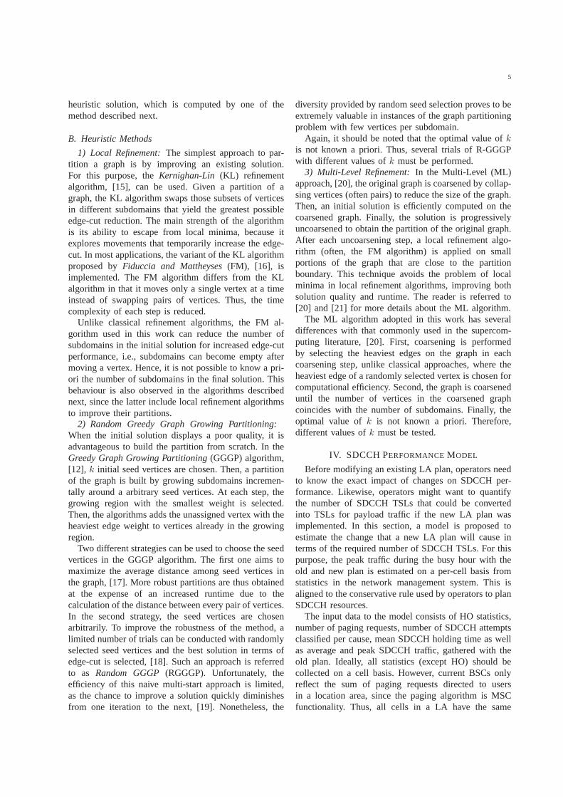
Hitherto, the analysis has justified the steps in theestimation process. The last figure shows the overallaccuracy of the model. Fig. 4 (a)-(b) shows a scatter plotof estimates versus measurements for weekly averages ofthe difference in average and peak SDCCH BH traffic.From the figures, it can be concluded that the model canestimate changes in the average SDCCH traffic caused bythe new LA plan quite accurately. However, it only givesa rough approximation of changes in the peak traffic.
B. Method Assessment
In spite of its limitations, the above-described modelis used to compare the performance of several graphpartitioning methods over real graphs. For this purpose,a larger geographical area is considered.
1) Analysis Set-up: The extended network area covers100000 km2, comprising 9807 BSs, 3353 sites, 76 BSCs,20 MSCs and 71 LAs. Statistical performance measure-ments were gathered for the whole area during 2 weeks.Table II shows some statistics of the area. From the table,it can be deduced that the number of TSLs devoted toSDCCH is 7% of total network capacity. An upper boundof the number of saved TSLs achieved by optimisingthe LA plan is the number of SDCCH TSLs in BSswith more than 1 TSL minus the minimum numberof SDCCH TSLs in these BSs (i.e., 6902-3237=3665).
TABLE II
STATISTICS IN THE SCENARIO WITH EXISTING CONFIGURATION.
Total nbr. of TSLs 202240Total nbr. of SDCCH TSLs 13472
Nbr. of BSs with NTSL > 1 3237Total nbr. of SDCCH TSLs in BSs with NTSL > 1 6902
Maximum BH paging load per LA [req./h] 134959Total sum of BH paging load [req./h] 5208060
Total sum of BH Avg. SDCCH traf. [E] 11294.2Total sum of Pk BH SDCCH traf. [E] 71300
Likewise, it is observed that the maximum paging loadper LA (i.e., 134959) is far from the maximum capacityvalue (i.e., 400000). This evidence clearly indicates thatthe size of LAs can be made at least three times largerwithout compromising paging performance. From thesum of paging load, it can be deduced that the minimumnumber of LAs is 14.
Although the area consisted of several MSCs, a singleinstance of the LA planning problems is considered, asit is assumed that the core network includes the featurethat allows LAs to cross MSC borders. The networkgraph is built from statistics collected during 2 weeks.Edge weights are computed by scaling the number ofHOs in 2 weeks by a factor 1/14 to reflect the dailyaverage. Vertex weights are the maximum number ofpaging requests originated in cells during the SDCCHBH in 2 weeks. As an optimization constraint, the sumof paging requests from cells in a LA must be below400000 (i.e., Baw=400000).
During the analysis, several methods are compared. Toquantify the improvement of a new LA plan, the initialoperator solution (denoted as OI for Operator Initial)is evaluated first. Then, several graph partitioning algo-rithms are tested: a) the BC algorithm over the ILP modelof the problem (denoted as BC), b) the FM refinement ofthe operator solution (denoted as FM), c) the traditionalML refinement algorithm (denoted as ML), and d) theRGGGP algorithm, based on the repeated use of GGGPwith random seed selection and FM refinement. Theexact method uses the BC algorithm in SCIP, [22],whereas the heuristic methods were implemented fromscratch in Matlab, [23]. In all heuristic methods, thenumber of passes in the FM refinement algorithm is 4.All methods are tested with different target values of k,ranging from 14 to 20, and the best solution is selected.Note that FM and ML are deterministic and, therefore,a single run is performed per value of k. In contrast,RGGGP is randomised and hence produces a differentsolution for each different random seed. Reported valuesfor RGGGP correspond to the best solution found in 100attempts per value of k.
During the comparison, heuristic methods are appliedto the graphs of site and BSC resolution. The exact
10
y = 1,045x + 0,085
R² = 0,760
-1
-0,5
0
0,5
1
1,5
2
-0,5 0 0,5 1 1,5 2
Measured difference in avg SDCCH traffic in BH
Estimated difference in avg SDCCH traffic in BH
y = 1,095x + 0,283
R² = 0,472
-3
-2
-1
0
1
2
3
4
5
6
-1 0 1 2 3 4
Measured difference in pk SDCCH traffic in BH
Estimated difference in peak SDCCH traffic in BH
(a) Average SDCCH traffic (b) Peak SDCCH traffic
Fig. 4. A scatter plot of measurements versus estimates of changes in SDCCH traffic.
method is only tested on the graph of BSC resolutionfor computational efficiency. Performance assessment isbased on solution quality in terms of edge-cut. By usingthe proposed performance model, edge-cut figures aretranslated into changes in SDCCH traffic and savedTSLs. Time efficiency is not considered in the analysisas it is not a critical issue, since LA re-planning isperformed, at most, once a week.
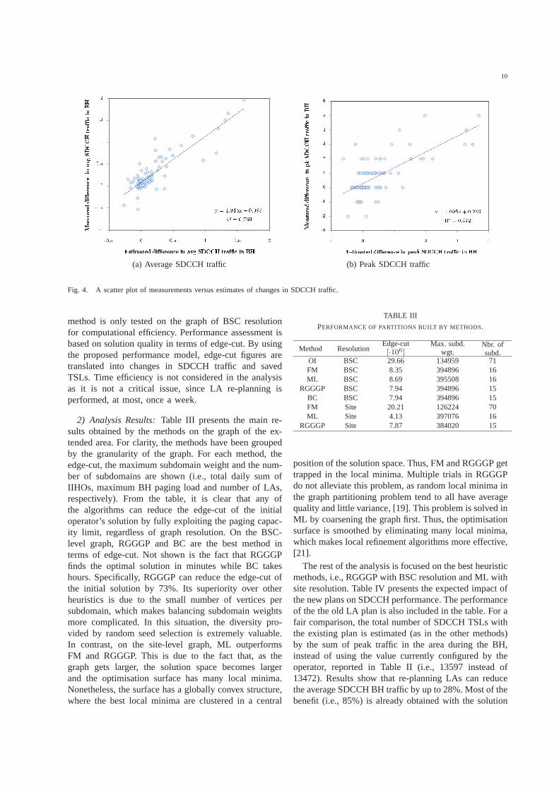
2) Analysis Results: Table III presents the main re-sults obtained by the methods on the graph of the ex-tended area. For clarity, the methods have been groupedby the granularity of the graph. For each method, theedge-cut, the maximum subdomain weight and the num-ber of subdomains are shown (i.e., total daily sum ofIIHOs, maximum BH paging load and number of LAs,respectively). From the table, it is clear that any ofthe algorithms can reduce the edge-cut of the initialoperator’s solution by fully exploiting the paging capac-ity limit, regardless of graph resolution. On the BSC-level graph, RGGGP and BC are the best method interms of edge-cut. Not shown is the fact that RGGGPfinds the optimal solution in minutes while BC takeshours. Specifically, RGGGP can reduce the edge-cut ofthe initial solution by 73%. Its superiority over otherheuristics is due to the small number of vertices persubdomain, which makes balancing subdomain weightsmore complicated. In this situation, the diversity pro-vided by random seed selection is extremely valuable.In contrast, on the site-level graph, ML outperformsFM and RGGGP. This is due to the fact that, as thegraph gets larger, the solution space becomes largerand the optimisation surface has many local minima.Nonetheless, the surface has a globally convex structure,where the best local minima are clustered in a central
RGGGP BSC 7.94 394896 15BC BSC 7.94 394896 15FM Site 20.21 126224 70ML Site 4.13 397076 16
RGGGP Site 7.87 384020 15
position of the solution space. Thus, FM and RGGGP gettrapped in the local minima. Multiple trials in RGGGPdo not alleviate this problem, as random local minima inthe graph partitioning problem tend to all have averagequality and little variance, [19]. This problem is solved inML by coarsening the graph first. Thus, the optimisationsurface is smoothed by eliminating many local minima,which makes local refinement algorithms more effective,[21].
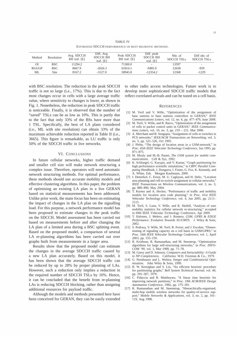
The rest of the analysis is focused on the best heuristicmethods, i.e., RGGGP with BSC resolution and ML withsite resolution. Table IV presents the expected impact ofthe new plans on SDCCH performance. The performanceof the the old LA plan is also included in the table. For afair comparison, the total number of SDCCH TSLs withthe existing plan is estimated (as in the other methods)by the sum of peak traffic in the area during the BH,instead of using the value currently configured by theoperator, reported in Table II (i.e., 13597 instead of13472). Results show that re-planning LAs can reducethe average SDCCH BH traffic by up to 28%. Most of thebenefit (i.e., 85%) is already obtained with the solution
11
TABLE IV
ESTIMATED SDCCH PERFORMANCE OF BEST HEURISTIC METHODS.
ML Site 8167.2 -3127.0 58945.8 -12354.2 12368 -1229
with BSC resolution. The reduction in the peak SDCCHtraffic is not so large (i.e., 17%). This is due to the factmost changes occur in cells with a large average trafficvalue, where sensitivity to changes is lower, as shown inFig. 1. Nonetheless, the reduction in peak SDCCH trafficis noticeable. Finally, it is observed that the number of“saved” TSLs can be as low as 10%. This is partly dueto the fact that only 33% of the BSs have more than1 TSL. Specifically, the best of LA plans considered(i.e., ML with site resolution) can obtain 33% of themaximum achievable reduction reported in Table II (i.e.,3665). This figure is remarkable, as LU traffic is only50% of the SDCCH traffic in live networks.
VI. CONCLUSIONS
In future cellular networks, higher traffic demandand smaller cell size will make network structuring acomplex issue. Therefore, operators will need automaticnetwork structuring methods. For optimal performance,these methods should use accurate mobility models andeffective clustering algorithms. In this paper, the problemof optimising an existing LA plan in a live GERANbased on statistical measurements has been addressed.Unlike prior work, the main focus has been on estimatingthe impact of changes in the LA plan on the signallingload. For this purpose, a network performance model hasbeen proposed to estimate changes in the peak trafficon the SDCCH. Model assessment has been carried outbased on measurements before and after changing theLA plan of a limited area during a BSC splitting event.Based on the proposed model, a comparison of severalLA re-planning algorithms has been carried out overgraphs built from measurements in a larger area.
Results show that the proposed model can estimatethe changes in the average SDCCH traffic caused bya new LA plan accurately. Based on this model, ithas been shown that the average SDCCH traffic canbe reduced by up to 28% by proper planning of LAs.However, such a reduction only implies a reduction inthe required number of SDCCH TSLs by 10%. Hence,it can be concluded that the benefit from re-planningLAs is reducing SDCCH blocking, rather than assigningadditional resources for payload traffic.
Although the models and methods presented here havebeen conceived for GERAN, they can be easily extended
to other radio access technologies. Future work is todevelop more sophisticated SDCCH traffic models thatreflect correlated arrivals and can be tuned on a cell basis.
REFERENCES
[1] M. Toril and V. Wille, “Optimization of the assignment ofbase stations to base stations controllers in GERAN,” IEEECommunications Letters, vol. 12, no. 6, pp. 477–479, June 2008.
[2] M. Toril, V. Wille, and R. Barco, “Optimization of the assignmentof cells to packet control units in GERAN,” IEEE Communica-tions Letters, vol. 10, no. 3, pp. 219 – 221, Mar 2006.
[3] A. Merchant and B. Sengupta, “Assignment of cells to switches inPCS networks,” IEEE/ACM Transactions on Networking, vol. 3,no. 5, pp. 521–526, Oct 1995.
[4] J. Plehn, “The design of location areas in a GSM-network,” inProc. 45th IEEE Vehicular Technology Conference, Jun 1995, pp.871–875.
[5] M. Mouly and M.-B. Pautet, The GSM system for mobile com-munications. Cell & Sys, 1992.
[6] K. Schloegel, G. Karypis, and V. Kumar, “Graph partitioning forhigh performance scientific simulations,” in CRPC Parallel Com-puting Handbook, J. Dongarra, I. Foster, G. Fox, K. Kennedy, andA. White, Eds. Morgan Kaufmann, 2000.
[7] I. Demirkol, C. Ersoy, M. U. Caglayan, and H. Delic, “Locationarea planning and cell-to-switch assignment in cellular networks,”IEEE Transactions on Wireless Communications, vol. 3, no. 3,pp. 880–890, May 2004.
[8] T. Kurner and A. Hecker, “Performance of traffic and mobilitymodels for location area code planning,” in Proc. 61st IEEEVehicular Technology Conference, vol. 4, Jun 2005, pp. 2111–2115.
[9] M. Toril, S. Luna, V. Wille, and R. Skehill, “Analysis of usermobility statistics for cellular network re-structuring,” acceptedin 69th IEEE Vehicular Technology Conference, Apr 2009.
[10] T. Halonen, J. Melero, and J. Romero, GSM, GPRS & EDGEPerformance: Evolution Towards 3G/UMTS. J. Wiley & Sons,2002.
[11] S. Pedraza, V. Wille, M. Toril, R. Ferrer, and J. Escobar, “Dimen-sioning of signaling capacity on a cell basis in GSM/GPRS,” inProc. 54th IEEE Vehicular Technology Conference, vol. 1, April2003, pp. 155–159.
[12] R. Krishnan, R. Ramanathan, and M. Steentrup, “Optimizationalgorithms for large self-structuring networks,” in Proc. INFO-COM ’99, vol. 1, Mar 1999, pp. 71–78.
[13] M. Garey and D. Johnson, Computers and Intractability: A Guideto NP-Completeness. California: W.H. Freeman & Co., 1979.
[14] G. Nemhauser and L. Wolsey, Integer and Combinatorial Opti-mization. John Wiley & Sons, 1999.
[15] B. W. Kernighan and S. Lin, “An efficient heuristic procedurefor partitioning graphs,” Bell System Technical Journal, vol. 49,pp. 291–307, 1970.
[16] C. Fiduccia and R. Mattheyses, “A linear time heuristic forimproving network partitions,” in Proc. 19th ACM/IEEE DesignAutomation Conference, 1982, pp. 175–181.
[17] R. Ramanathan and M. Steenstrup, “Hierarchically-organized,multi-hop mobile wireless networks for quality-of-service sup-port,” Mobile Networks & Applications, vol. 3, no. 2, pp. 101–119, Aug 1998.
12
[18] G. Karypis and V. Kumar, “A fast and high quality multilevelscheme for partitioning irregular graphs,” SIAM Journal onScientific Computing, vol. 20, no. 1, pp. 359–392, 1998.
[19] K. D. Boese, A. Khang, and S. Muddu, “A new adaptive multi-start technique for combinatorial global optimizations,” Opera-tion Research Letters, vol. 16, pp. 101–113, 1994.
[20] G. Karypis and V. Kumar, “Multilevel k-way partitioning schemefor irregular graphs,” Journal of Parallel and Distributed Com-puting, vol. 48, no. 1, pp. 96–129, 1998.
[21] C. Walshaw, “Multilevel refinement for combinatorial optimisa-tion problems,” Annals of Operations Research, vol. 131, pp.325–372, 2004.
[22] T. Achterberg, “SCIP - a framework to integrate constraintand mixed integer programming,” Zuse Institute Berlin, Tech.Rep. TR 04-19, 2004, http://www.zib.de/Publications/abstracts/ZR-04-19/.
[23] The MathWorks, Inc., “Getting started with Matlab (version 6),”July 2002, available at http://www.mathworks.com.