Performance and Cost Analysis of a Structured Concrete ...

University of Arkansas, FayettevilleScholarWorks@UARK

Theses and Dissertations

12-2012

Performance and Cost Analysis of a StructuredConcrete Thermocline Thermal Energy StorageSystemMatt Nicholas StrasserUniversity of Arkansas, Fayetteville

Follow this and additional works at: http://scholarworks.uark.edu/etd

Part of the Civil Engineering Commons, and the Power and Energy Commons

This Thesis is brought to you for free and open access by ScholarWorks@UARK. It has been accepted for inclusion in Theses and Dissertations by anauthorized administrator of ScholarWorks@UARK. For more information, please contact [email protected], [email protected].

Recommended CitationStrasser, Matt Nicholas, "Performance and Cost Analysis of a Structured Concrete Thermocline Thermal Energy Storage System"(2012). Theses and Dissertations. 627.http://scholarworks.uark.edu/etd/627

http://scholarworks.uark.edu?utm_source=scholarworks.uark.edu%2Fetd%2F627&utm_medium=PDF&utm_campaign=PDFCoverPages

http://scholarworks.uark.edu/etd?utm_source=scholarworks.uark.edu%2Fetd%2F627&utm_medium=PDF&utm_campaign=PDFCoverPages

http://scholarworks.uark.edu/etd?utm_source=scholarworks.uark.edu%2Fetd%2F627&utm_medium=PDF&utm_campaign=PDFCoverPages

http://network.bepress.com/hgg/discipline/252?utm_source=scholarworks.uark.edu%2Fetd%2F627&utm_medium=PDF&utm_campaign=PDFCoverPages

http://network.bepress.com/hgg/discipline/274?utm_source=scholarworks.uark.edu%2Fetd%2F627&utm_medium=PDF&utm_campaign=PDFCoverPages

http://scholarworks.uark.edu/etd/627?utm_source=scholarworks.uark.edu%2Fetd%2F627&utm_medium=PDF&utm_campaign=PDFCoverPages

mailto:[email protected],%[email protected]

PERFORMANCE AND COST ANALYSIS OF A STRUCTURED CONCRETE THERMOCLINE THERMAL ENERGY STORAGE SYSTEM

PERFORMANCE AND COST ANALYSIS OF A STRUCTURED CONCRETE THERMOCLINE THERMAL ENERGY STORAGE SYSTEM

A thesis submitted in partial fulfillment of the requirements for the degree of

Master of Science in Civil Engineering

By

Matthew N. Strasser Harding University

Bachelor of Science in Mechanical Engineering, 2011

December 2012 University of Arkansas

ABSTRACT

Increasing global energy demands and diminishing fossil fuel resources have raised increased

interest in harvesting renewable energy resources. Solar energy is a promising candidate, as

sufficient irradiance is incident to the Earth to supply the energy demands of all of its

inhabitants. At the utility scale, concentrating solar power (CSP) plants provide the most cost-

efficient method of harnessing solar energy for conversion to electrical energy. A major

roadblock to the large-scale implementation of CSP plants is the lack of thermal energy storage

(TES) that would allow the continued production of electricity during the absence of constant

irradiance. Sensible heat TES has been suggested as the most viable form of TES for CSP

plants. Two-tank fluid TES systems have been incorporated at several CSP plants, significantly

enhancing the performance of the plants. A single-tank thermocline TES system, requiring a

reduced liquid media volume, has been suggested as a cost-reducing alternative. Unfortunately,

the packed-aggregate bed of such TES system introduces the issue of thermal ratcheting and

rupture of the tank’s walls. To address this issue, it has been suggested that structured concrete

be used in place of the aggregate bed. Potential concrete mix designs have been developed and

tested for this application. Finite-difference-based numeric models are used to study the

performance of packed-bed and structured concrete thermocline TES systems. Optimized

models are developed for both thermocline configurations. The packed-bed thermocline model

is used to determine whether or not assuming constant fluid properties over a temperature range

is an acceptable assumption. A procedure is developed by which the cost of two-tank and single-

tank thermocline TES systems in the capacity range of 100-3000 MWhe can be calculated.

System Advisory Model is used to perform life-cycle cost and performance analysis of a central

receiver plant incorporating four TES scenarios: no TES, two-tank TES, packed-bed thermocline

TES, and structured concrete thermocline TES. Conclusions are drawn as to which form of TES

provides the most viable option. Finally, concrete specimens cast from the aforementioned mix

designs are tested in the presence of molten solar salt, and their applicability as structured filler

material is assessed.

This thesis is approved for recommendation to the Graduate Council.

Thesis Director:

_______________________________________ Dr. R. Panneer Selvam

Thesis Committee:

_______________________________________ Dr. Micah Hale

_______________________________________

Dr. Ernest Heymsfield

THESIS DUPLICATION RELEASE

I hereby authorize the University of Arkansas Libraries to duplicate this thesis when needed for research and/or scholarship.

Agreed _______________________________________ Matthew N. Strasser

Refused _______________________________________

Matthew N. Strasser

ACKNOWLEDGMENTS

I must first and foremost thank God for granting me the desire and capability to do this

work; without him, nothing is possible (Proverbs 25:2, Philippians 4:13).

I would like to express the deepest gratitude for my advisor Dr. Panneer Selvam. He has

been an excellent mentor, helping to educate me, not only in my area of research, but about the

research process as a whole. Our many talks about areas of life ranging from religion to politics

and the economy have definitely expanded my diversity of thought. Our work within this thesis

has been a definite success, and I look forward to our success in the upcoming years.

I would like to thank Dr. Micah Hale and Dr. Ernest Heymsfield for serving on my

committee and providing valuable suggestions and criticism.

I am most grateful for my colleagues that worked on this project before me: Marco

Castro, Joel Skinner, Brad Brown, and Emerson John. Their work provided a solid foundation

from which I could build.

I would like to thank technicians Mark Kuss and David Peachee for their help in

operating, trouble-shooting, and repairing the testing equipment used in this work.

Lastly, I would like to acknowledge and thank the Department of Energy for funding and

supporting my research efforts.

DEDICATION

I would like to dedicate this thesis to my parents, Fred and Rebecca Strasser. They have

been very supportive of me and encouraged me to pursue my interests and strive for excellence

in what I do. Thank you for providing me with the opportunity to excel.

TABLE OF CONTENTS

CHAPTER 1: INTRODUCTION AND THESIS OBJECTIVES .................................................. 1

1.1 Introduction ...................................................................................................................... 1

1.2 Thesis Objectives ............................................................................................................. 7

CHAPTER 2: LITERATURE REVIEW ...................................................................................... 10

2.1 Introduction ......................................................................................................................... 10

2.2 Concentrating Solar Power: Methods of Collection .......................................................... 10

2.2.1 Dish .............................................................................................................................. 10

2.2.2 Linear Concentrators.................................................................................................... 11

2.2.3 Central Receiver........................................................................................................... 14

2.3 Primary Methods of TES .................................................................................................... 15

2.3.1 Chemical TES .............................................................................................................. 16

2.3.2 Latent Heat TES........................................................................................................... 17

2.3.3 Sensible Heat TES ....................................................................................................... 21

2.4 Sensible Heat TES System Classification........................................................................... 28

2.4.1 Passive Sensible Heat TES .......................................................................................... 28

2.4.2 Active Sensible Heat TES............................................................................................ 31

2.4.3 Indirect and Direct Sensible Heat TES ........................................................................ 34

2.4.4 Single and Dual Media TES Systems .......................................................................... 36

2.5 CSP Power Plants Incorporating TES................................................................................. 39

2.5.1 Direct TES CSP Power Plants ..................................................................................... 40

2.5.2 Indirect TES CSP Power Plants ................................................................................... 44

2.6 TES System Cost Estimation .............................................................................................. 45

2.7 Conclusions from Literature Review and Motivation for Thesis ....................................... 48

CHAPTER 3: MODELING OF THERMOCLINE TES SYSTEMS ........................................... 51

3.1 1D Packed-Bed Thermocline Model (PBTC) ..................................................................... 53

3.1.1 Schumann Equation and Assumptions......................................................................... 53

3.1.2 Numeric Formulation of PBTC Model ........................................................................ 58

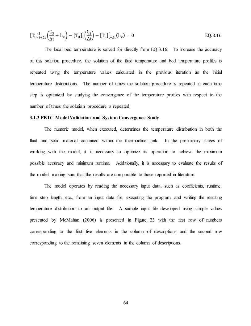
3.1.3 PBTC Model Validation and System Convergence Study .......................................... 64

3.1.4 Impact of Temperature-Dependent Fluid Properties on PBTC Model ........................ 71

3.1.5 PBTC Models: Limestone Bed and Quartzite Bed ...................................................... 76

3.2 2D Structured Concrete Thermocline (SCTC) Model ........................................................ 78

3.2.1 SCTC Model and Assumptions ................................................................................... 80

3.3 Overview of System Advisory Model ................................................................................ 90

3.3.1 Studies to be conducted with SAM.............................................................................. 91

3.3.2 Works in Literature Validating the Performance of SAM ........................................... 92

3.3.3 Using SAM to Study Impact of Different Sensible Heat TES Systems ...................... 94

CHAPTER 4: EVALUATION OF CONCRETE FOR A STRUCTURED CONCRETE

THERMOCLINE ........................................................................................................................ 103

4.1 Considerations for Concrete for High Temperature Applications .................................... 103

4.1.1 Structural Compatibility of Concrete with High Temperatures................................. 104

4.1.2 Chemical Compatibility of Concrete with Molten Salt ............................................. 105

4.2 Evaluation of Mix Designs ............................................................................................... 106

4.2.1 Testing of Concrete Specimens at Elevated Temperatures........................................ 106

4.2.2 4 Concrete Mix Designs for Lab-Scale Testing......................................................... 108

4.3 Testing of Concrete Beam Specimens .............................................................................. 109

4.3.1 Lab-Scale Test System............................................................................................... 109

4.3.2 Selection and Construction of Concrete Specimens for Lab-Scale Testing .............. 112

4.3.3 Testing Procedure ...................................................................................................... 114

CHAPTER 5: RESULTS AND DISCUSSION.......................................................................... 116

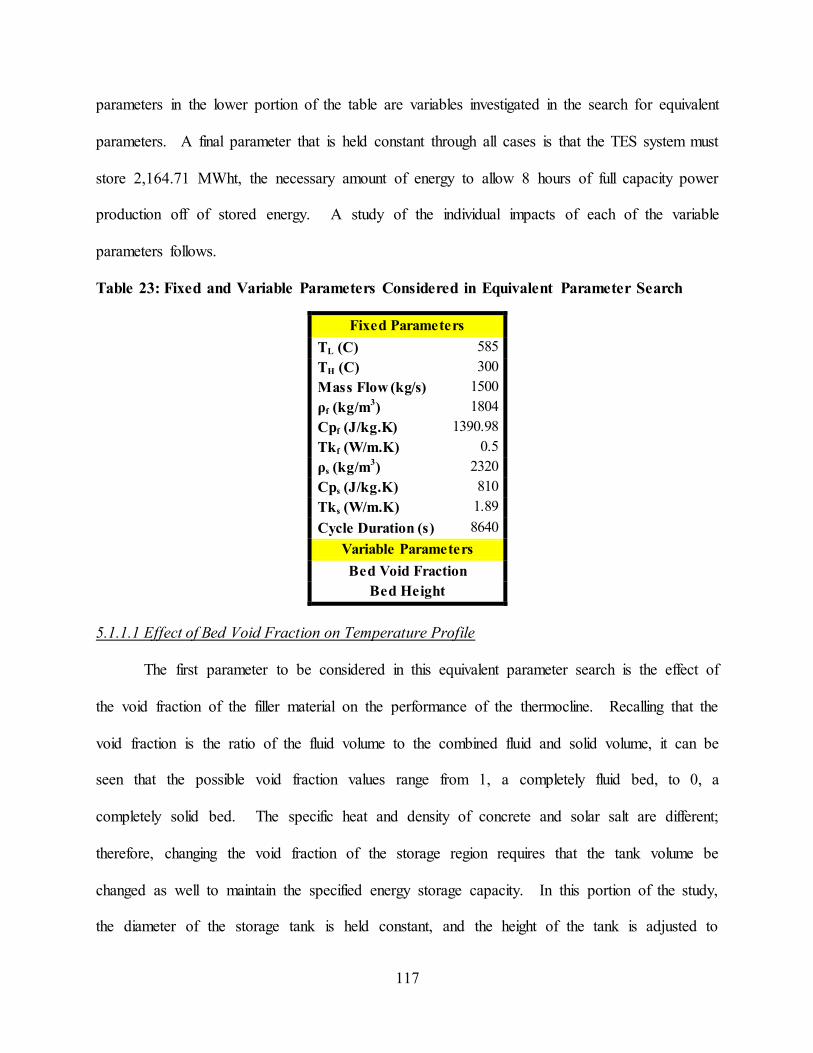
5.1 Equivalent Parameters between PBTC and SCTC Models .............................................. 116

5.1.1 Sensitivity Analysis ................................................................................................... 116

5.1.2 Impact of Number of Nodes Used on Performance of PBTC Model ........................ 120

5.1.2 Equivalence between PBTC Model and Brown’s SCTC Model ............................... 122

5.1.3 Equivalence between PBTC Case I and SCTC Case I .............................................. 125

5.2 SAM Modeling Results..................................................................................................... 128

5.2.1 Scenario One: No TES .............................................................................................. 128

5.2.2 Scenario Two: Two-Tank Molten Salt TES ............................................................. 130

5.2.3 Scenario Three: Quartzite Packed-Bed Thermocline TES ....................................... 132

5.2.4 Scenario Four: Structured Concrete Thermocline .................................................... 134

5.2.5 Summary and Comparison of TES Scenarios............................................................ 136

5.3 Testing of Concrete Mix Designs ..................................................................................... 138

5.3.1 Problems Encountered During Testing of Concrete Specimens ................................ 138

5.3.2 Testing of Mix 26 (TC1000) ...................................................................................... 143

5.3.3 Testing of Mix 11 (40FA-60CA) ............................................................................... 144

CHAPTER 6: CONCLUSIONS ................................................................................................. 146

6.1 Conclusions ....................................................................................................................... 146

6.2 Suggestions for Future Work ............................................................................................ 148

WORKS CITED ......................................................................................................................... 150

COURSEWORK AND PUBLICATIONS ................................................................................. 156

APPENDIX A: PACKED BED THERMOCLINE MODEL ..................................................... 157

User’s Manual ......................................................................................................................... 157

Input File ............................................................................................................................. 157

Output Files......................................................................................................................... 157

Source Code ............................................................................................................................ 158

APPENDIX B: PACKED BED THERMOCLINE MODEL (VARRIABLE PROPERTIES) .. 161

User’s Manual ......................................................................................................................... 161

Input File ............................................................................................................................. 161

Output File .......................................................................................................................... 161

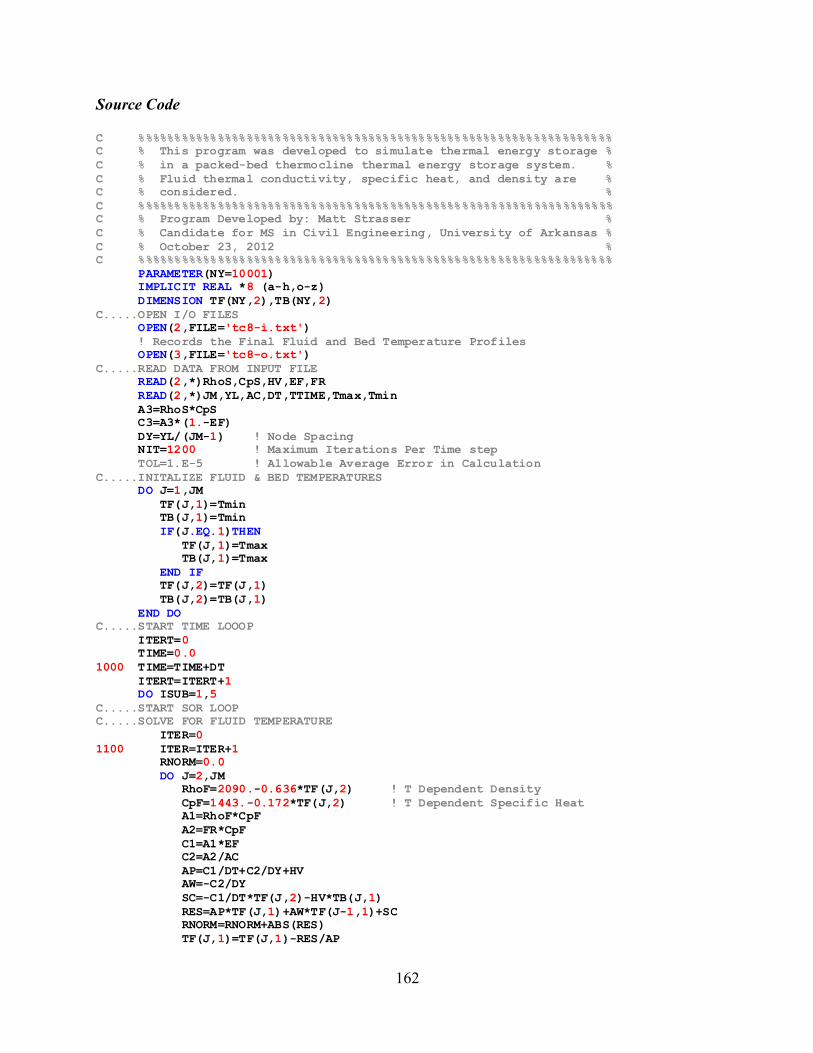
Source Code ............................................................................................................................ 162

LIST OF FIGURES

Figure 1: Yearly United States Energy Consumption by Sources (EIA, Energy Perspectives, 2009) ............................................................................................................................................... 1

Figure 2: Prototype 150 kW Dish Plant at National Solar Thermal Test Facility (Fraser, 2005) 11 Figure 3: Parabolic Troughs from the 280 MW Power Plant Solana under Construction in Gila Bend, AZ (Siemens, 2009)............................................................................................................ 12

Figure 4: Linear Fresnel Array at the 30 MW Puerto Errado 2 CSP Plant in Calasparra, Spain (PE2, 2010) ................................................................................................................................... 14

Figure 5: Central Receiver and Heliostats at the 20 MW PS20 Plant in Seville, Spain (Molina, 2009) ............................................................................................................................................. 15 Figure 6: Shell and Tube PCM Configuration (Aggenim et al., 2010)......................................... 21

Figure 7: Un-insulated 20 m3 Concrete Block-and-Tube TES Unit tested by Laing at DLR-German Aerospace Center (Laing et al., 2006) ............................................................................ 30

Figure 8: Cracking in Concrete Block with No Soft Material at Interface of Concrete and Stainless Steel Heat Exchanger (Skinner et al., 2011) .................................................................. 31 Figure 9: Illustration of Two-Tank Liquid Media TES System (Hammerschlag, Pratt, Schaber, &

Widergren, 2006) .......................................................................................................................... 32 Figure 10: Illustration of Single Tank Thermocline TES (Hammerschlag et al., 2006) .............. 33

Figure 11: Temperature Profile in Single-Tank Thermocline TES System during Discharging (Left to Right with Time) (Xu et al., 2012) .................................................................................. 34 Figure 12: Parabolic Trough CSP Power Plant Incorporating Two-Tank AIS (EPRI, 2010) ...... 35

Figure 13: Central Receiver CSP Power Plant Incorporating Two-Tank ADS (EPRI, 2010) ..... 36 Figure 14: Schematic of Packed Bed Thermocline with Fluid Flow Directions Labeled (Xu et al.,

2012) ............................................................................................................................................. 38 Figure 15: Energy Storage Tank at 10 MW Central Receiver ADS Plant in Seville, Spain (Medrano et al., 2010)................................................................................................................... 40

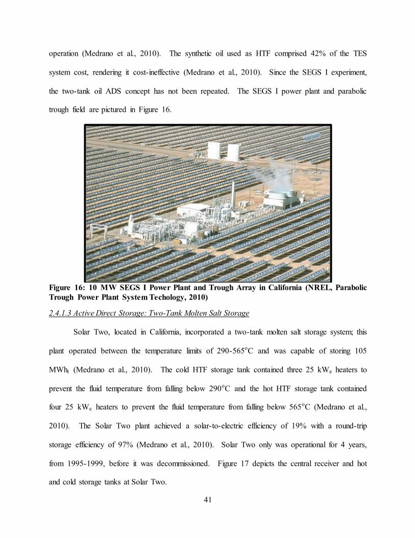
Figure 16: 10 MW SEGS I Power Plant and Trough Array in California (NREL, Parabolic Trough Power Plant System Techology, 2010) ............................................................................ 41

Figure 17: Central Receiver and Hot and Cold HTF Tanks at Solar Two in California (NASS, 2012) ............................................................................................................................................. 42 Figure 18: Central Receiver and Energy Storage Tanks at 19.9 MW Gemasolar Plant in Seville,

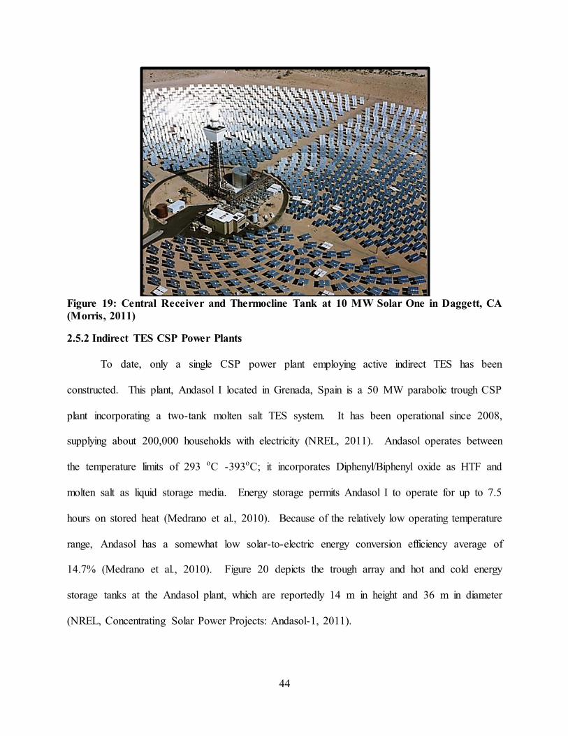
Spain (Harrington, 2012) .............................................................................................................. 43 Figure 19: Central Receiver and Thermocline Tank at 10 MW Solar One in Daggett, CA (Morris,

2011) ............................................................................................................................................. 44 Figure 20: Two-Tank TES and Trough Array at 50 MW Andasol I in Grenada, Spain (Craig, 2011) ............................................................................................................................................. 45

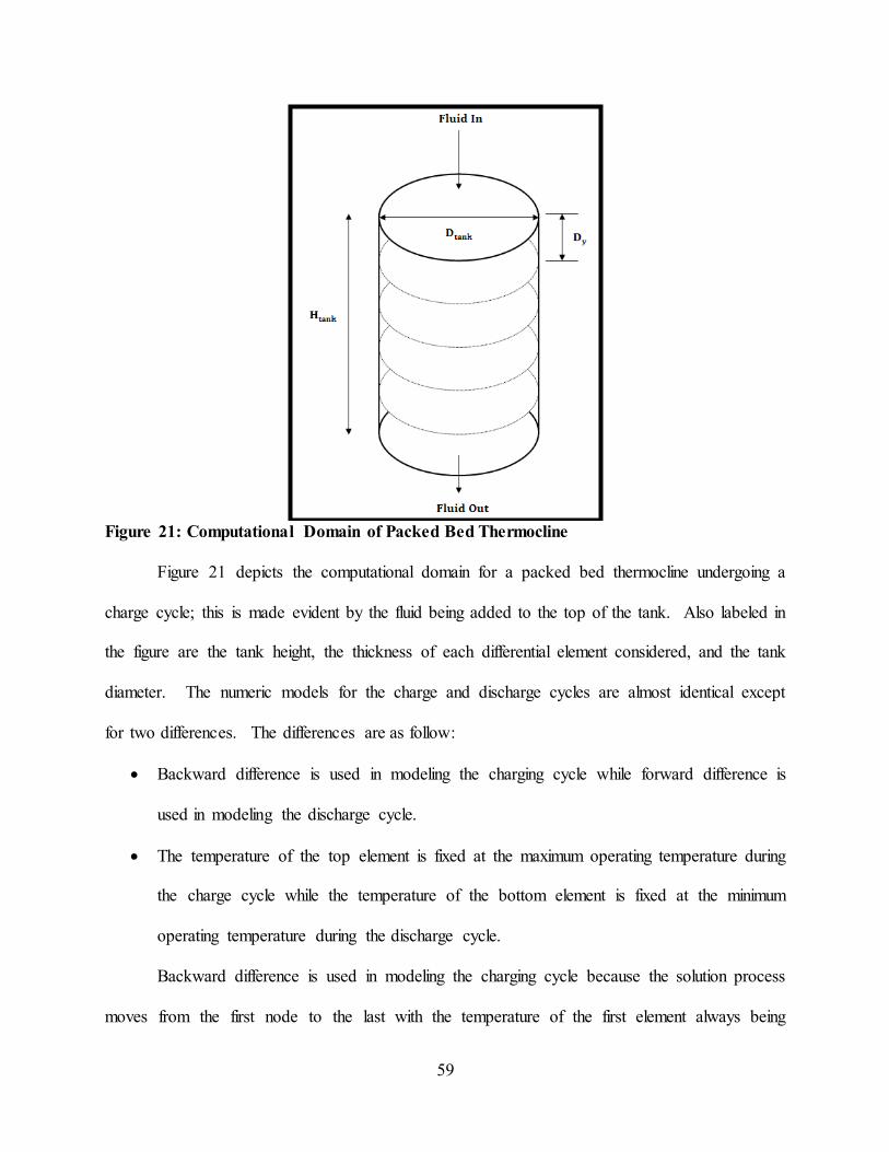
Figure 21: Computational Domain of Packed Bed Thermocline .................................................. 59 Figure 22: Fluid and Solid Temperatures Used in Computing Element 2’s Temperature during

Charge Cycle (Colored Elements Indicate Known Solid and Fluid Temperatures) ..................... 61 Figure 23: Sample Input File for PBTC Model ............................................................................ 65 Figure 24: Comparison of Charge Cycle Temperature Profiles from Literature (Left) and from

the PBTC Model (Right) (Pacheco et al., 2002) ........................................................................... 65 Figure 25: Inlet and Outlet Fluid Temperatures during 3.5 Hour Charge Cycle from Literature

(Left) and from the PBTC Model (Right) (Pacheco et al., 2002) ................................................. 66 Figure 26: Impact of Time Step on Temperature Profile .............................................................. 68

Figure 27: Convergence of Temperature Profile with Increased Number of Nodes .................... 69 Figure 28: Impact of Number of Repetitions of Calculating Fluid and Bed Temperatures ......... 71

Figure 29: Temperature Profiles Generated Using Constant (Solid Line) and Variable (Dashed Line) Fluid Properties during Six-Hour Charge Cycle: 290oC-390oC (Left) and 290oC-565oC

(Right) ........................................................................................................................................... 74 Figure 30: Temperature Profiles Generated Using Constant (Solid Line) and Variable (Dashed Line) Fluid Properties during Four-Hour Charge Cycle: 290oC-390oC (Left) and 290oC-565oC

(Right) ........................................................................................................................................... 75 Figure 31: Charge (Right) and Discharge (Left) Temperature Profiles for PBTC Thermocline

Case I, Limestone Bed .................................................................................................................. 77 Figure 32: Charge (Right) and Discharge (Left) Temperature Profiles for PBTC Thermocline Case II, Quartzite Bed ................................................................................................................... 77

Figure 33: Cross Sectional View of Thermocline Tank Populated with Parallel Plate Structured Concrete (View from Above) (Brown et al., 2012) ...................................................................... 79

Figure 34: Two Concrete Plates and One Fluid Flow Channel (Hatched Region Indicates Computational Domain) (Brown et al., 2012) .............................................................................. 80 Figure 35: Input Files for Charge (Left) and Discharge (Right) Cycles (Brown, 2012) .............. 83

Figure 36: Temperature Profiles for Charge (Left) and Discharge (Right) Cycles Using Brown’s (2012) Optimized Parallel Plate Model ........................................................................................ 84

Figure 37: Energy Stored (Left) During Charge Cycle and Energy Retrieved (Right) During Discharge Cycle ............................................................................................................................ 84 Figure 38: Optimized Input Files for Charge (Left) and Discharge (Right) Cycles (Case I) ....... 86

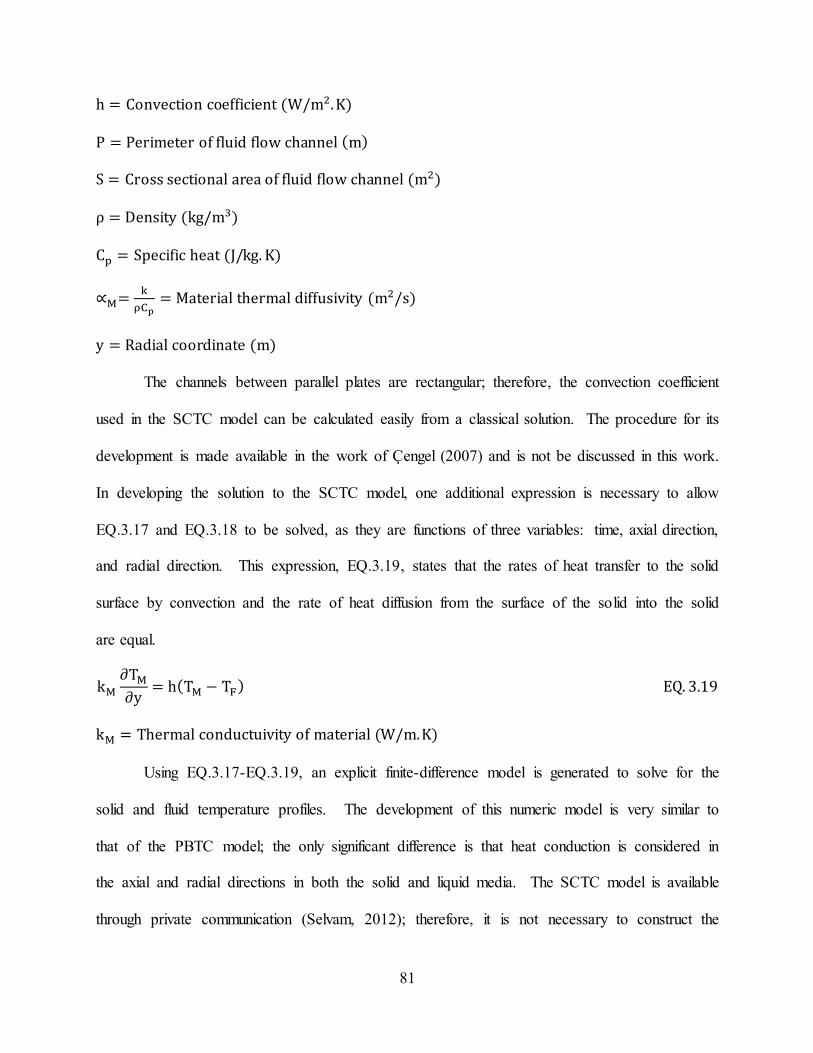
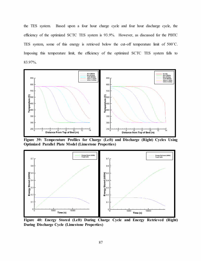
Figure 39: Temperature Profiles for Charge (Left) and Discharge (Right) Cycles Using Optimized Parallel Plate Model (Limestone Properties) .............................................................. 87

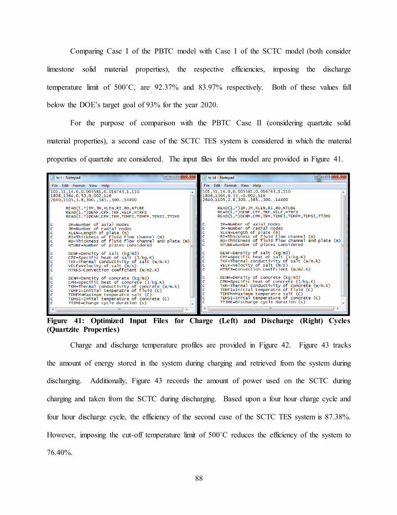
Figure 40: Energy Stored (Left) During Charge Cycle and Energy Retrieved (Right) During Discharge Cycle (Limestone Properties) ...................................................................................... 87 Figure 41: Optimized Input Files for Charge (Left) and Discharge (Right) Cycles (Quartzite

Properties) ..................................................................................................................................... 88 Figure 42: Temperature Profiles for Charge (Left) and Discharge (Right) Cycles Using

Optimized Parallel Plate Model (Quartzite Properties) ................................................................ 89 Figure 43: Energy Stored (Left) During Charge Cycle and Energy Retrieved (Right) During Discharge Cycle (Quartzite Properties) ........................................................................................ 89

Figure 44: Comparison of Measured and Modeled Heat from Trough Collector Field (Wagner et al., 2011) ....................................................................................................................................... 92

Figure 45: Tank Cost for Thermocline Tank (Blue) and Two-Tank (Red) TES Systems............ 99 Figure 46: Oven Damaged While Heating Concrete Specimen (Left) and Cylinder Cage Damaged While Heating Specimen (Right) (John, 2012) .......................................................... 104

Figure 47: Concrete Specimens in Molten Salt Bath (John, 2012)............................................. 107 Figure 48: Dimensioned Schematic of Lab-Scale Thermocline Test System ............................ 110

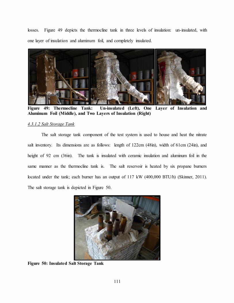
Figure 49: Thermocline Tank: Un-insulated (Left), One Layer of Insulation and Aluminum Foil (Middle), and Two Layers of Insulation (Right) ........................................................................ 111 Figure 50: Insulated Salt Storage Tank....................................................................................... 111

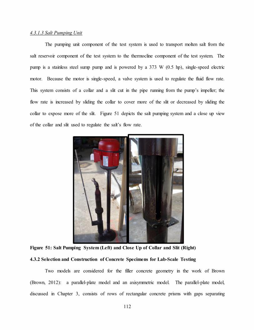
Figure 51: Salt Pumping System (Left) and Close Up of Collar and Slit (Right) ...................... 112 Figure 52: Assembled Test System during Testing .................................................................... 115

Figure 53: Effect of Void Fraction on Charge Cycle Temperature Profile ................................ 118 Figure 54: Effect of Tank Height on Charge Cycle Temperature Profile ................................... 120

Figure 55: Effect of Changing the Number of Nodes on Charge Temperature Profile .............. 122 Figure 56: Charge Cycle Temperature Profile from PBTC Case I (Left) and Brown's SCTC

Model (Right).............................................................................................................................. 123 Figure 57: Comparison of PBTC Case I (Dotted Line), Brown’s SCTC Model (Dashed Line),

and PBTC Model Using 17 Nodes (Solid Line) ......................................................................... 124 Figure 58: Comparison of SCTC Case I (Dotted Line), SCTC Case I (Dashed Line), and PBTC Model Using 35 Nodes ............................................................................................................... 127

Figure 59: Nominal LCOE of CSP Plant with No TES .............................................................. 129 Figure 60: Monthly Electrical Output for CSP Plant with No TES............................................ 130

Figure 61: Nominal LCOE of CSP Plant with Two-Tank TES .................................................. 131 Figure 62: Monthly Electrical Output for CSP Plant with Two-Tank TES................................ 132 Figure 63: Nominal LCOE of CSP Plant with Packed-Bed Thermocline TES .......................... 133

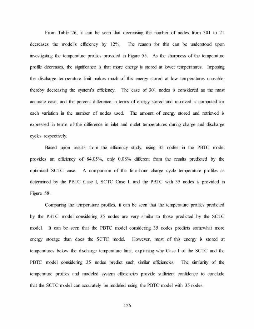
Figure 64: Monthly Electrical Output for CSP Plant with Packed-Bed Thermocline TES ........ 134 Figure 65: Nominal LCOE of CSP Plant with Structured Thermocline TES ............................. 135

Figure 66: Monthly Electrical Output for CSP Plant with Structured Thermocline TES .......... 136 Figure 67: Salt Frozen in Lines during Testing .......................................................................... 140 Figure 68: Heating Frozen Thermocline Test Chamber (Left) and Cleared Thermocline Chamber

with Concrete/Salt Blockage on the Ground (Right) .................................................................. 141 Figure 69: Motor Driving Pumping Unit During Testing (Left) and Pumping Unit Being

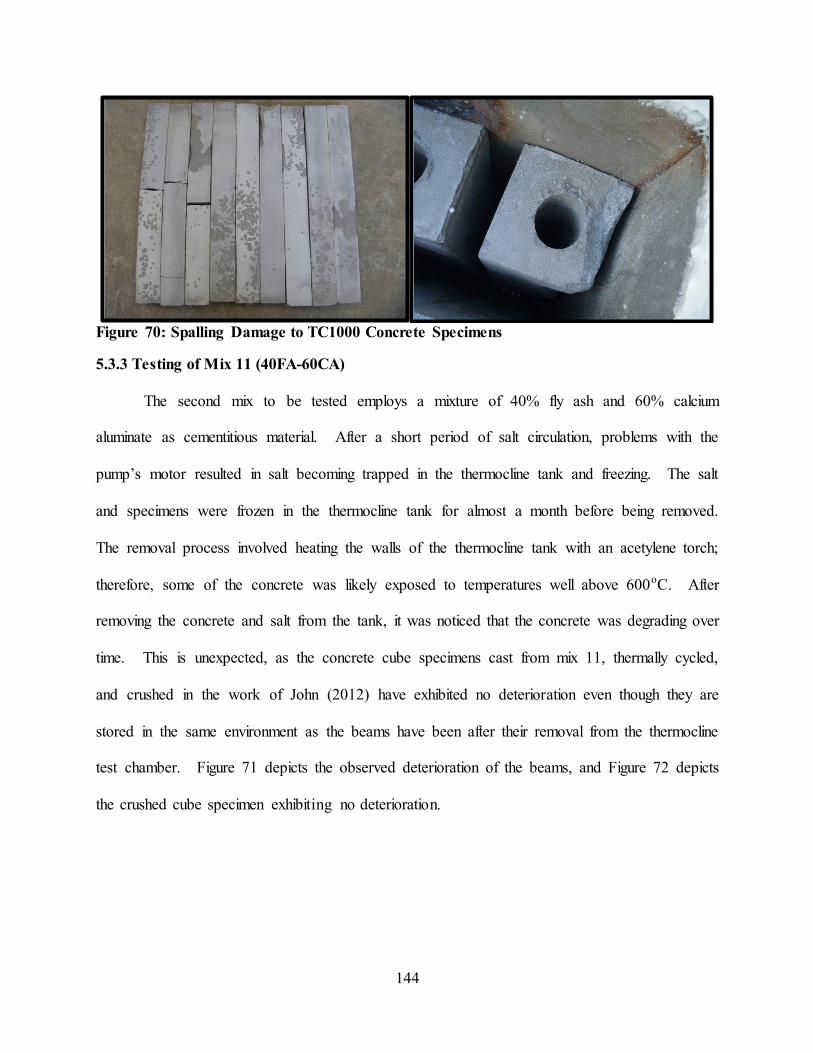
Removed to Allow Replacement of First Motor (Right) ............................................................ 143 Figure 70: Spalling Damage to TC1000 Concrete Specimens ................................................... 144 Figure 71: Progressive Deterioration of Mix 11 Specimens: 1 Month After Testing (Left) and 3

Months After Testing (Right) ..................................................................................................... 145 Figure 72: Crushed Mix 11 Specimen Exhibiting no Deterioration more than 1 Year After

Thermal Cycling ......................................................................................................................... 145

LIST OF TABLES

Table 1: Cost of Electricity and Capacity Factor for Various Technologies (EIA, 2012) .............. 2 Table 2: Energy Storage Cost Comparison of Various Technologies (Schoenung, 2011)............. 4

Table 3: Potential CES Materials and Reaction Information (Gil, et al., 2010) ........................... 17 Table 4: Commonly-Used Liquid TES Media and Properties (Herrmann & Kearney, 2002) ..... 24 Table 5: Reduction in TES Costs through Incorporation of Salt as Liquid Media (Kearney, et al.,

2002) ............................................................................................................................................. 25 Table 6: Composition, Melting Point, and Cost of Three Commonly-Used Nitrate Salts

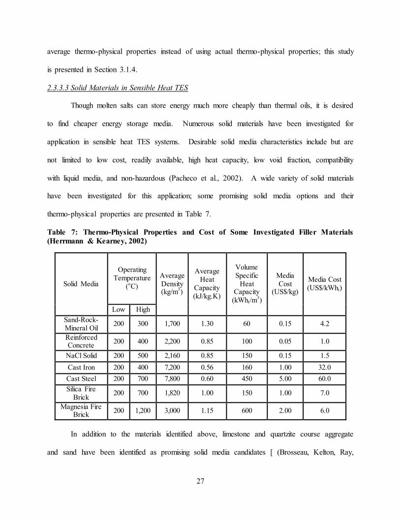
(Kearney, et al., 2002)................................................................................................................... 25 Table 7: Thermo-Physical Properties and Cost of Some Investigated Filler Materials (Herrmann & Kearney, 2002).......................................................................................................................... 27

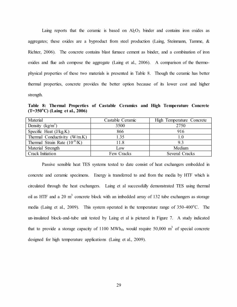
Table 8: Thermal Properties of Castable Ceramics and High Temperature Concrete (T=350oC) (Laing et al., 2006) ........................................................................................................................ 29

Table 9: EPRI Cost Estimation of Two-Tank TES Systems Based on Capacity (EPRI, 2010) ... 47 Table 10: EPRI Cost Estimation of Thermocline TES Systems Based on Capacity (EPRI, 2010)....................................................................................................................................................... 48

Table 11: Properties Held Constant for All Models ..................................................................... 72 Table 12: Constant Properties for Case I: Mass Flow Rate of 900 kg/s ...................................... 73

Table 13: Constant Properties for Case II: Mass Flow Rate of 1500 kg/s ................................... 75 Table 14: Material Properties of Materials Considered for Bed of PBTC ................................... 76 Table 15: Comparison of Recorded and Simulated Performance of SEGS VI CSP Power Plant

(Price, 2003).................................................................................................................................. 93 Table 16: SAM Base Case Plant, Field, and Receiver Parameters ............................................... 95

Table 17: Tank and Media Costs for Two-Tank and Thermocline TES Systems ........................ 98 Table 18: Average Thermo-Physical Properties and Costs of Liquid and Solid Media ............. 100 Table 19: Direct Cost Contributions, Excluding Tank and Media, and Direct Cost Subtotal .... 101

Table 20: Indirect Cost Contributions and Indirect Cost Subtotal.............................................. 101 Table 21: TES System Costs and Unit Capacity Cost Values for Input in SAM ....................... 102

Table 22: Average Properties of Concrete Mix Designs Selected for Testing (John, 2012) ...... 108 Table 23: Fixed and Variable Parameters Considered in Equivalent Parameter Search ............ 117 Table 24: Parameters in 1D Model Affected by Void Fraction of Bed ...................................... 118

Table 25: Parameters in 1D Model Affected by Height of Bed ................................................. 119 Table 26: Decrease in Efficiency of PBTC Model with Decrease in Number of Nodes............ 125

Table 27: Performance Summary for CSP Plant with No TES .................................................. 130 Table 28: Performance Summary for CSP Plant with Two-Tank TES ...................................... 132 Table 29: Performance Summary for CSP Plant with Packed-Bed Thermocline TES .............. 134

Table 30: Performance Summary for CSP Plant with Structured Thermocline TES ................. 136 Table 31: Cost and Performance of 100 MWe CSP Plant with Different TES Configurations..... 137

NOMENCLATURE

Variables

Ac = Cross sectional area of tank (m2)

As,shape = Surface area of shape being considered (m2)

As,sphere = Surface area of sphere with equivalent volume to shape being considered (m2)

α = Surface area shape factor (dimensionless)

αM = Thermal diffusivity of concrete (m2/s)

Cp = Specific heat capacity (J/kg.K)

CpF,avg = Average fluid specific heat (J/kg.K)

D = Sphere diameter (m)

ε = Void fraction of bed (dimensionless)

h = Convection coefficient (W/m2.K)

hv = Interstitial heat transfer coefficient (W/m3.K)

k = Thermal conductivity (W/m.K)

kF,avg = Average fluid thermal conductivity (W/m.K)

m = Mass (kg)

= Mass flow rate (kg/s)

Nu,sphere = Nusselt number for flow over a sphere (dimensionless)

P = Perimeter of fluid flow channel (m)

Pr = Prandlt number (dimensionless)

ρ = Density (kg/m3)

ρf = Average of fluid densities at surface and free stream temperatures (kg/m3)

Q = Stored energy (J)

rsphere = Radius of sphere with equivalent volume to shape under consideration (m)

Re = Reynolds number (dimensionless)

S = Cross sectional area of fluid flow channel (m2)

t = time (s)

T = Temperature (K or ˚C)

TB = Temperature of bed material (˚C)

TM = Temperature of concrete material (˚C)

TF = Temperature of heat transfer fluid (˚C)

ΔT = Temperature change (K or ˚C)

µ = Viscosity (kg/m.s)

µavg = Average of fluid viscosity at surface and free stream temperatures (kg/m.s)

µ∞ = Viscosity at free stream temperature (kg/m.s)

µs = Viscosity at surface temperature (kg/m.s)

vavg = Average fluid velocity (m/s)

V = Fluid flow velocity (m/s)

VB = Solid material volume in bed region of tank (m3)

VF = Fluid material volume in bed region of tank (m3)

Numeric Model Variables

A1 = (ρCp)F

A2 = ( Cp)F

A3 = (ρCp)B

C1 = εA1

C2 = A2/Ac

C3 = (1-ε)A3

Subscript ‘t’ = Corresponds to current time step

Subscript ‘t+1’ = Corresponds to upcoming time step

Superscript ‘J’ = Corresponds to element whose temperature is being solved for

Superscript ‘J-1’ = Corresponds to element preceding the element currently being solved

Δt = Time step (s)

Δy = Node spacing (m)

LIST OF ACRONYMS

CSP = Concentrating Solar Power

DOE = Department of Energy

EIA = Energy Information Administration

EPRI = Electric Power Research Institute

HTF = Heat Transfer Fluid

HPC = High Performance Concretes

IEA = International Energy Agency

LCOE = Levelized Cost of Electricity

LHS = Latent Heat Storage

NREL = National Renewable Energy Laboratories

NSTTF = National Solar Thermal Test Facility

PBTC = Packed Bed Thermocline

PCM = Phase Change Material

SAM = System Advisory Model

SCTC = Structured Concrete Thermocline

SNL = Sandia National Laboratories

TES = Thermal Energy Storage

TRNSYS = Transient System Simulation Tool

1

CHAPTER 1: INTRODUCTION AND THESIS OBJECTIVES

1.1 Introduction

The population of the world is increasing at a rapid rate; increasing with the population is

the global energy demand. According the Energy Information Administration (EIA), the amount

of energy consumed by the average United States citizen increased by 44% between 1949 and

2009 (from 214-308 million Btu or 226-336 TJ) (Energy Perspectives, 2009). The vast majority

of this energy is supplied by fossil fuels (EIA, Energy Perspectives, 2009). As the United States’

population continues to increase, it can be assumed that the general energy consumption trend,

pictured in Figure 1, will continue.

Figure 1: Yearly United States Energy Consumption by Sources (EIA, Energy

Perspectives, 2009)

A nation’s energy supply is a matter of national security and stability; without a reliable

power grid, the operation of critical facilities such as hospitals and military installations can be

put in jeopardy. Unfortunately, the United States has not been energy self-sufficient since the

1950’s, importing more than 60% of the oil it consumes (SNL, 2011). To attain increased

national security and a stable energy supply to drive national growth in the future, it is

imperative that the United States diversify its energy supply to include alternative, renewable

energy sources. Table 1 provides a comparison of the cost of producing electricity using various

2

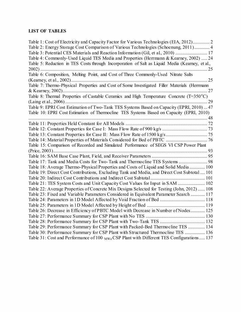
technologies, using both renewable and nonrenewable resources, and the associated capacity

factors of these technologies.

Table 1: Cost of Electricity and Capacity Factor for Various Technologies (EIA, 2012)

Source of Power for Production

of Electricity

Cost Prediction (2010 $) for 2017

Average LCOE

(¢/kWht)

Capacity Factor

(%)

Coal

Conventional 9.96 ¢ 85.00%

Advanced 20.39 ¢ 85.00%

Natural Gas

Conventional Combined Cycle 6.18 ¢ 87.00%

Advanced Combined Cycle 5.89 ¢ 87.00%

Conventional Combustion Turbine 9.46 ¢ 30.00%

Advanced Combustion Turbine 8.04 ¢ 30.00%

Wind

Inshore 9.68 ¢ 34.00%

Offshore 33.06 ¢ 27.00%

Solar

Photovoltaic 15.69 ¢ 25.00%

Thermal 25.1 ¢ 20.00%

Nuclear 11.27 ¢ 90.00%

Geothermal 9.96 ¢ 92.00%

Biomass 12.02 ¢ 83.00%

Hydro 8.99 ¢ 53.00%

Solar energy is a promising potential alternative energy source. The earth’s atmosphere

continuously receives a mean irradiance of about 1.35 kW/m2, leading to a net energy reception

rate of 1.7(10)17 W; however, much of this energy is absorbed or scattered in the atmosphere

(Goswami, Kreith, & Kreider, 2000). The mean irradiance of the Earth is much smaller,

reportedly varying from 150-300 W/m2 (Goswami et al., 2000). If less than 1% of the Earth’s

irradiance could be harvested and converted at 10% efficiency, sufficient energy would be

produced to exceed the needs of the world’s population (Goswami et al., 2000).

Solar radiation is harvested in one of two ways: it is collected by photovoltaic cells and

directly converted to electricity using semiconductors or it is concentrated and captured and used

3

to drive a steam power cycle. Photovoltaic systems currently available on the market generally

range in efficiency between 12-20% (EIA, 2009). Conversion efficiencies of up to 43.5% have

been achieved in lab-scale testing (Wesoff, 2011); however, such photovoltaic systems are not

cost competitive for large-scale power production at this time. Concentrating solar power (CSP)

plants have been recognized as a possible supplier of the large quantities of needed electrical

energy (Xu, Wang, He, Li, & Bai, 2012).

One problem plaguing the large-scale implementation of CSP plants is the intermittent

nature of irradiance at any given location on the Earth (Brown, Strasser, & Selvam, 2012). The

Earth’s irradiance varies due to factors such as the position of the sun, cloud cover and density,

etc. and is absent at night. For CSP plants to be implemented on a large scale, their capacity

factors will have to be improved by finding a way to guarantee a steady heat source to the plant

amid unsteady irradiance. The key to operation with fluctuating irradiance is to incorporate

thermal energy storage (TES) into the power plants. TES can function as a capacitor, increasing

the temperature of the liquid media when solar irradiance is not intense enough to heat it to

desired levels, or act as a battery, allowing the power plant to continue producing power well

after the sun has set (Adinberg, Zvegilsky, & Epstein, 2010).

A reasonable question, regarding the necessity of TES, is why not increase the capacity

of the plant and store the excess electrical power produced for use when solar irradiance is not

available. The answer to this question is that storing electrical energy is considerably more

expensive than storing energy in alternative forms and generating the electric power as needed.

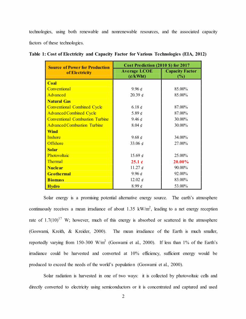
A comparison of energy storage technologies is provided in Table 2.

4

Table 2: Energy Storage Cost Comparison of Various Technologies (Schoenung, 2011)

Technology $/kWh Efficiency

SLA Battery $330.00 80.00%

LI Battery $600.00 85.00%

Super Capacitor $10,000.00 95.00%

HS Flywheel $1,600.00 95.00%

Pumped Hydro $75.00 85.00%

Sensible Heat $31.00 93.00%

TES systems considered for application in a CSP plant fall under one of three categories:

sensible heat storage, phase change storage, or chemical storage (Tahat, Babus'Haq, &

O'Callaghan, 1993). Sensible heat storage systems have been suggested as the most practical

method of energy thermal energy storage (Herrmann & Kearney, 2002); currently, all power

plants incorporating TES employ sensible heat storage.

Sensible heat is defined as the amount of energy released from a material as its

temperature is increased or decreased (Gil, et al., 2010). Most sensible heat TES systems operate

by elevating the temperature of a volume of liquid media and storing it for later use. These

systems can be classified into one of the following two categories: two-tank, in which hot and

cold liquid media are stored in separate tanks, and single-tank, thermocline systems, in which

both hot and cold liquid media are stored in the same tank. In either system, one of the most

costly components is the liquid media inventory [ (Herrmann & Kearney, 2002) and (Pacheco,

Showalter, & Kolb, 2002)]. Filler materials are currently being investigated to reduce the

necessary volume of liquid media, thereby decreasing the cost of sensible heat TES. Concrete

has been suggested as a potential TES media, providing storage at the cost of $1/kWht

(Herrmann & Kearney, 2002).

Some level of testing of concrete as TES media has been conducted. One concept

involved casting a steel heat exchanger in a concrete block and circulating thermal oil through

5

the heat exchanger in the temperature range of 300oC-400oC (Laing, Lehmann, FiB, & Bahl,

2009). A similar concept involved casting a steel heat exchanger in concrete prisms and

circulating molten salt through the heat exchanger in the elevated temperature range of 450o-

500oC (Skinner, Brown, & Selvam, 2011). However, due to the high cost of stainless steel heat

exchangers necessary to avoid deterioration from the corrosive salt, this concept is not cost

effective (Skinner et al., 2011). A proposed, cost-decreasing alternative is a single-tank

thermocline TES, using molten salt as the liquid media and geometrically-optimized, structured

concrete filler material (Brown et al., 2012).

It is ideal for TES systems to operate at the maximum possible temperature, as this

increases the energy storage density of the system and the efficiency of the Rankine power cycle

executed by power plants (Kearney, et al., 2002). Unfortunately, concrete is susceptible to spall

or explode at temperatures exceeding 300˚C. (John, Hale, & Selvam, 2011). High performance

concretes (HPCs) have been designed and reported to sustain thermal cycling at temperatures of

up to 600oC, demonstrating their potential as filler material in a sensible heat TES application

(John et al., 2011). Significant modeling work has been conducted to optimize the geometry of

the filler concrete using a 2D heat transfer model developed based upon the work of Schmidt and

Willmott (1981) and is reported by Brown [ (Brown et al., 2012) and (Brown, 2012)].

This work focuses on the optimization as well as cost and performance evaluation of a

single-tank thermocline TES system incorporating a binary molten salt (60% KNO3 40% NaO3)

as liquid media and structured HPC as a filler material. Previous work reports a maximum TES

system efficiency of 65.59% (Brown, 2012); this value falls significantly short of the DOE’s goal

of 93% for the year 2020. Modeling is re-investigated with the goal of optimizing a TES system

to attain efficiency at or exceeding the DOE’s goal.

6

System Advisory Model (SAM), a product of NREL, is used to simulate the life-cycle

performance of a CSP plant incorporating the optimized structured concrete thermocline TES

system. The thermocline modeling function in SAM is adapted from Transient System

Simulation Tool (TRNSYS). This thermocline model is developed based on the 1D Schumann

equation and valid for modeling packed bed thermocline systems composed of small particles.

In this work, a packed bed thermocline model based upon this 1D model is developed and its

results are compared with those of the 2D structured concrete thermocline model. A procedure is

discussed by which the input data of the packed bed model can be modified to attain similar

performance to that predicted by the 2D structured concrete thermocline model. This allows the

simulation of a structured concrete thermocline using SAM’s 1D thermocline function. A study

is conducted in which the accuracy of assuming constant versus variable fluid properties is

assessed.

To attain a comparison of the performance of this TES configuration with other sensible

heat configurations, three other configurations are considered: no TES, packed-bed thermocline

TES, and two-tank liquid TES. To allow the simulation of these TES scenarios, a procedure is

developed to determine a unit capacity cost for thermocline and two-tank TES systems in the

range of 100-3000 MWht. Conclusions are drawn as to whether a structured concrete

thermocline is a viable TES option.

John (2012) suggested concrete mix designs as possible candidates for filler material in a

structured concrete thermocline TES system. Beams are cast from each of these mix designs and

subjected to testing in circulating molten salt; the performance of these beams is assessed based

upon deterioration. Conclusions are drawn as to whether the concrete mix designs are ready for

testing in an actual thermocline system.

7

1.2 Thesis Objectives

Following the introductory chapter of this thesis, a comprehensive literature review is

provided in Chapter 2. The literature review discusses the three categories of TES with a

concentration on sensible heat thermal energy storage. Within the field of sensible heat TES

emphasis is placed on thermocline TES systems. A review and discussion of TES systems

incorporated at CSP plants, both presently and in the past, is also presented. Following this

literature review, the primary objectives of the thesis, as presented below, are addressed.

Objective 1: Evaluate previous studies conducted to optimize the geometry of structured filler

material in a concrete thermocline TES system. If possible, optimize the geometry further to

attain improved TES system efficiency.

In the work of Brown (2012), the geometry of structured concrete filler material was

optimized to attain a TES system efficiency of 65.59%; this is well short of the DOE’s

goal of 93% for the year 2020. If higher efficiencies cannot be attained, this TES concept

is not viable. The optimization work conducted by Brown will be investigated and new

modeling will be conducted to determine if increased system efficiency is attainable.

Objective 2: Perform a comparative cost and performance analysis of a CSP plant

incorporating a structured concrete thermocline TES system.

SAM, a product of NREL, allows the simulation of a power plant incorporating various

forms of TES; the software performs lifecycle cost and performance analysis. SAM will

be attained from NREL and used to study the impact of various TES configurations on

the cost and performance of a central receiver CSP plant.

SAM’s thermocline model is a 1D two-phase simulation, using the Schumann equation to

describe heat transfer between solid and fluid material. The model developed to study

8

the structured concrete thermocline is a 2D two-phase model. The 2D model considers

radial heat transfer; therefore, it can be inferred that the temperature distributions

predicted by the two models may not be the same. However, if SAM is to be used to

study a CSP plant with a structured concrete thermocline TES system, it must be possible

to analyze the structured concrete thermocline with the 1D model and attain similar

results as predicted by the 2D model.

o A 1D thermocline model will be developed, using the Schumann equation to

describe interstitial heat transfer, so that the temperature distributions calculated

by the thermocline model used in SAM may be compared with the results of the

2D model used to study the structured concrete thermocline.

o If temperature profiles and TES system efficiencies predicted by the 1D and 2D

models vary significantly, a process will be developed to attain similar

temperature distributions from the 1D model as produced by the 2D model.

SAM does not calculate the cost of the TES system. When using SAM, the user specifies

a plant capacity and the desired number of hours of operation on stored energy; based

upon these inputs, SAM determines the required storage capacity in MWht for the plant.

From this storage capacity, it is necessary to determine the capacity cost, or cost per

kilowatt-hour of TES. Therefore, it is necessary to establish a means of calculating the

TES capacity cost for both two-tank and single-tank thermocline TES systems.

Objective 3: Determine if assuming constant fluid properties is an acceptable assumption.

In this work, molten solar salt is the liquid media considered; its properties, such as

viscosity, density, and specific heat at constant pressure vary widely with temperature. In

most works found in literature, it is assumed that using the properties based upon the

9

middle temperature of the operating range (300˚C-400˚C) provides sufficient accuracy.

However, as the temperature range is increased, such as that considered in this work

(300˚C-585˚C), the variation of the properties from those at the median temperature

increases. The amount of error attained by assuming constant properties will be

investigated graphically using the 1D thermocline model.

Objective 4: Conduct performance evaluations of concrete mix designs developed for

application in a structured concrete thermocline TES system.

Based on the work of John (2012), concrete mixture designs have been specified as

potential candidates for application in a structured concrete thermocline. Small cube

specimens were tested by John in constant temperature and thermal cycling in the

presence of both molten salt and air. This testing involved heating the specimens in an

oven where the whole specimen was heated at a uniform rate; therefore, it is not known

how concrete specimens made from these mix designs will respond to stresses induced by

thermal gradients. A laboratory test system has been designed and constructed; concrete

beam specimens will be cast from two of John’s proposed four mix designs and subjected

to thermal cycling in this test system. The performance of the members will be evaluated

to determine if the concrete mix designs are still probable candidates for TES media in a

structured thermocline.

10

CHAPTER 2: LITERATURE REVIEW

2.1 Introduction

The purpose of this literature review is to identify and discuss the methods in which solar

energy is collected and stored; an emphasis is placed on sensible heat thermal energy storage

(TES). The review begins by discussing the three major methods of collecting and concentrating

solar radiation. Examples of power plants incorporating each method of energy collection are

discussed as well. Following the discussion of energy collection methods, the three major

categories of TES are discussed. Examples of existing TES systems are presented as their type is

discussed. The focus of this work is sensible heat storage; therefore, this is the major area of

discussion. Existing sensible heat storage systems are presented and discussed, along with heat

transfer fluids (HTFs) and solid media used in these systems.

2.2 Concentrating Solar Power: Methods of Collection

Thermal energy collection for fueling electricity production can be classified into one of

three major categories: Dish, Linear Concentrator, or Central Receiver (Brosseau et al., 2005).

2.2.1 Dish

Dish systems use a curved, reflective dish to track the sun and focus its radiation on a

receiver located above the dish. This receiver uses the heat energy to produce electricity by

executing a Stirling cycle. This method of energy concentration leads to operational

temperatures of up to 800oC (DOE, 2008). Partially due to this high operating temperature, dish

systems are the most efficient electricity-producing CSP technology, reportedly providing a

solar-to-electrical conversion efficiency of up to 25-30% (IEA, 2010). The current small size of

typical dish systems, most producing in the range of 3-25 kW, makes their near-term application

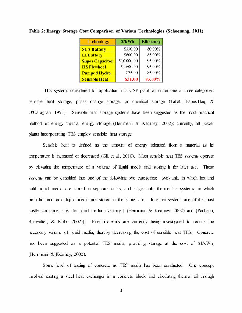
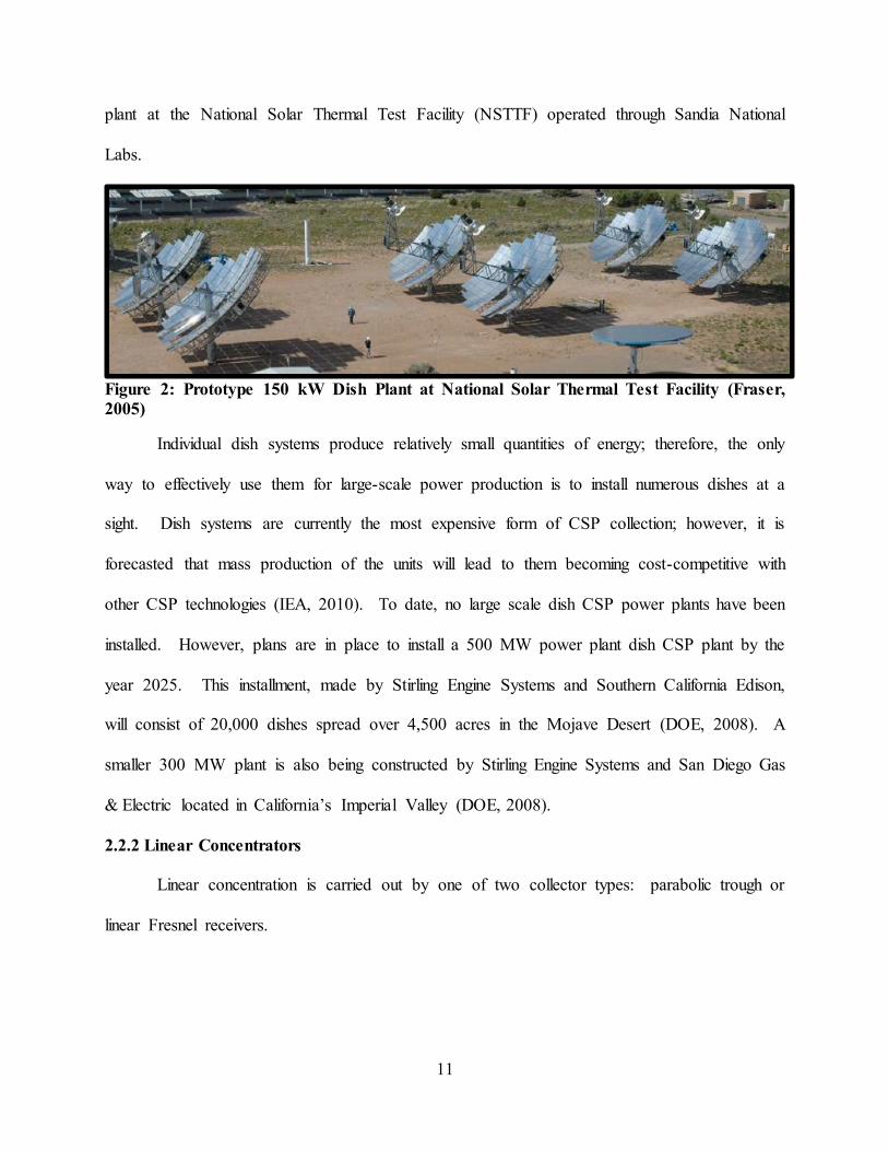
for primarily niche markets (DOE, 2008). Pictured in Figure 2 depicts a pilot scale dish power

11

plant at the National Solar Thermal Test Facility (NSTTF) operated through Sandia National

Labs.

Figure 2: Prototype 150 kW Dish Plant at National Solar Thermal Test Facility (Fraser,

2005)

Individual dish systems produce relatively small quantities of energy; therefore, the only

way to effectively use them for large-scale power production is to install numerous dishes at a

sight. Dish systems are currently the most expensive form of CSP collection; however, it is

forecasted that mass production of the units will lead to them becoming cost-competitive with

other CSP technologies (IEA, 2010). To date, no large scale dish CSP power plants have been

installed. However, plans are in place to install a 500 MW power plant dish CSP plant by the

year 2025. This installment, made by Stirling Engine Systems and Southern California Edison,

will consist of 20,000 dishes spread over 4,500 acres in the Mojave Desert (DOE, 2008). A

smaller 300 MW plant is also being constructed by Stirling Engine Systems and San Diego Gas

& Electric located in California’s Imperial Valley (DOE, 2008).

2.2.2 Linear Concentrators

Linear concentration is carried out by one of two collector types: parabolic trough or

linear Fresnel receivers.

12

2.2.2.1 Parabolic Trough

Parabolic trough collectors are composed of rows, of curved mirrors with a fixed stainless

steel tube suspended at the mirror’s focal point. Collection troughs sizes vary up to 100 m in

length and five to six meters across (IEA, 2010). As the troughs track the sun, HTF is circulated

through the tubes and heated by the concentrated solar radiation. The tubes are coated with

materials to increase degree to which they absorb the radiation; additionally, they are incased in

evacuated glass tubes to decrease radiation losses (IEA, 2010). Troughs are capable of heating

the HTF to temperatures of up to 390oC. Parabolic troughs are a well-developed and mature

technology, as they have been in use for over twenty years (EPRI, 2010). Reported thermal-to-

electrical efficiencies for parabolic trough systems reach 15% (IEA, 2010). The majority of CSP

plants in use today employ parabolic trough receivers (DOE, 2008). Figure 3 depicts the trough

array at Solana in Gila Bend, AZ.

Figure 3: Parabolic Troughs from the 280 MW Power Plant Solana under Construction in

Gila Bend, AZ (Siemens, 2009).

Currently, 11 CSP plants are in operation in the United States, falling under the size

range of 1-80 MW (NREL, 2011). Numerous CSP trough power plants are currently under

13

construction in the United States. Examples include the Solana Plant (Figure 3) and the Palen

Solar Power Project. The Solana plant, scheduled to come online in 2013, spans 1,920 acres and

is projected to supply 70,000 households with energy; when completed, it will be the largest

parabolic trough CSP plant in operation in the world (Abengoa, 2012). The prominence of

Solana amongst parabolic trough plants will be short lived, however, because the 500 MW Palen

Solar Power Project located near Desert Center, California is scheduled to come online in 2014

(NREL, 2010). When completed, the Palen Project will replace Solana as the largest parabolic

trough power plant in operation.

2.2.2.2 Linear Fresnel

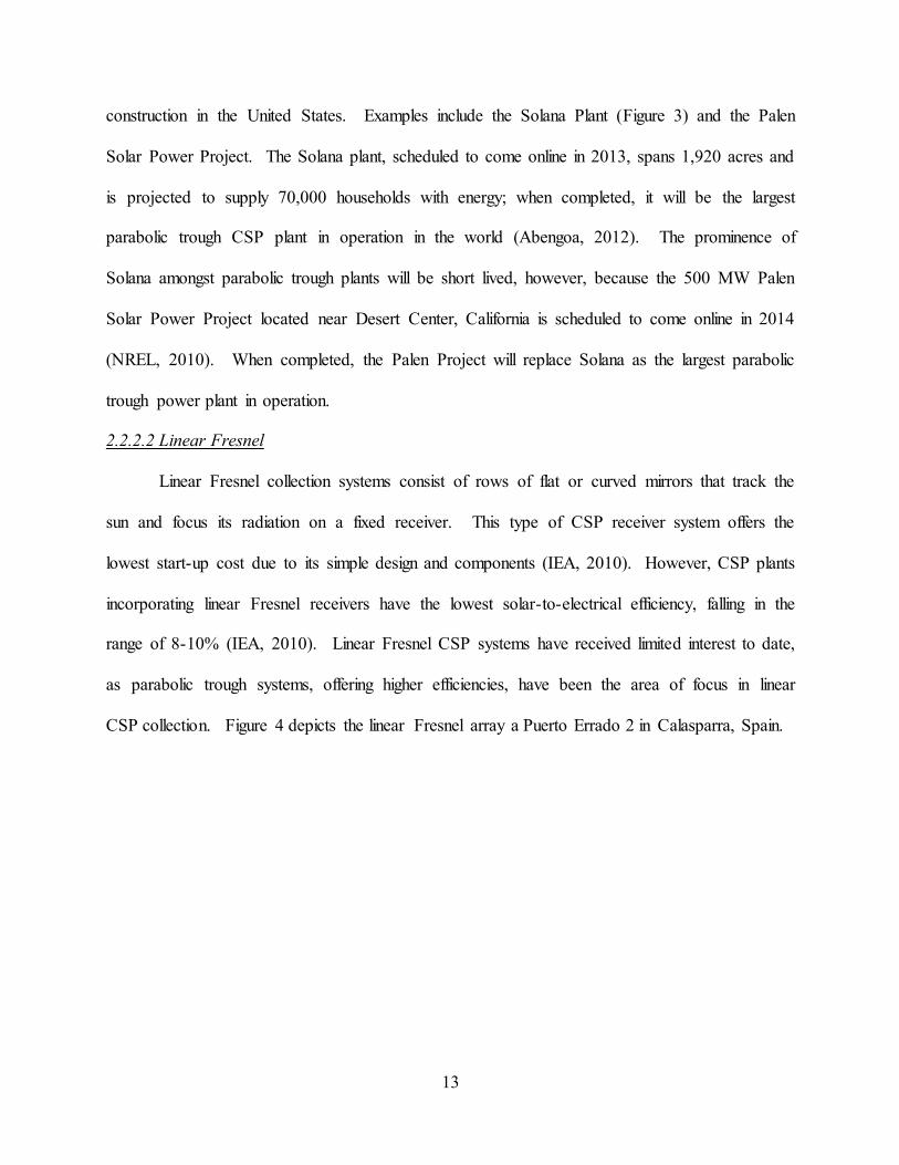
Linear Fresnel collection systems consist of rows of flat or curved mirrors that track the

sun and focus its radiation on a fixed receiver. This type of CSP receiver system offers the

lowest start-up cost due to its simple design and components (IEA, 2010). However, CSP plants

incorporating linear Fresnel receivers have the lowest solar-to-electrical efficiency, falling in the

range of 8-10% (IEA, 2010). Linear Fresnel CSP systems have received limited interest to date,

as parabolic trough systems, offering higher efficiencies, have been the area of focus in linear

CSP collection. Figure 4 depicts the linear Fresnel array a Puerto Errado 2 in Calasparra, Spain.

14

Figure 4: Linear Fresnel Array at the 30 MW Puerto Errado 2 CSP Plant in Calasparra,

Spain (PE2, 2010)

Puerto Errado 2 (PE2) has been in operation since March 2012; it is currently the largest

linear Fresnel CSP plant in operation (CleanEnergy, 2012). PE2 occupies almost 173 acres

(NREL, 2011), and the solar collection field contains over 302,000 m2 of aperture area

(NovatecSolar, 2012). PE2 is projected to supply 15,000 households with energy (NovatecSolar,

2012). Efforts are currently underway to reduce the production cost of the Fresnel lenses used in

Linear Fresnel CSP plants to make this technology more viable.

2.2.3 Central Receiver

Central receiver (power tower) collection systems consist of a field of flat mirror panels,

known as heliostats, which track the sun and focus solar radiation on an elevated central

receiving tower. Heliostats range in size, up to an area of 125 m2; receiver towers also vary in

size, up to the height of 165 m (Abengoa, PS20, the Largest Solar Power Tower Worldwide,

2012). Central receiver units typically collect heat at temperatures of up to 565oC (DOE, 2008);

however, potential operating temperatures in the 1000oC-1300oC range have been reported

(Romero, Buck, & Pacheco, 2002). Due to these high operating temperatures, the solar-to-

15

electrical efficiency of central receiver CSP plants is reportedly in the range of 20-35% (IEA,

2010). The large range in efficiency variation is due to the difference in the typical operating

temperature of 565oC and the potential range of 1000oC-1300oC. Figure 5 depicts the tower and

heliostat array of PS20 in Seville, Spain.

Figure 5: Central Receiver and Heliostats at the 20 MW PS20 Plant in Seville, Spain

(Molina, 2009)

PS20 has been operational since 2009; it is currently the largest central receiver CSP

power plant in operation. Its solar collection field spans 210 acres and is composed of 1255 120

m2 heliostats; the central receiver, stands at a height of 165 m (Abengoa, 2012). PS20

reportedly provides sufficient energy for 10,000 households (Abengoa, 2012).

2.3 Primary Methods of TES

A major problem faced by solar power plants today is the intermittent nature of the solar

energy supply. Fluctuations in the supply of heat from the collectors to the power blocks in the

power plants lead to non-constant power production. Additionally, CSP plants that have not

been constructed as hybrids, with backup fossil fuel supplies, are forced to go offline during

nighttime hours. Integrating TES into CSP plants solves the aforementioned problems. The

16

ability to incorporate reasonably cheap TES into CSP plants gives them a significant advantage

over renewable technologies such as photovoltaic or wind turbines; it is much cheaper to store

heat energy and generate electricity as it is needed than it is to generate the electricity and store it

until it is needed (Herrmann & Kearney, 2002).

Stored thermal energy allows the continued operation of the plant’s power block after the

sun sets. Due to cloud cover, contamination in the air, etc., the supply of heat from the collector

field fluctuates. Stored thermal energy can increase the plant’s efficiency by maintaining the

temperature of the HTF flow from the collector field at the desired operating temperature for the

power block (Laing et al., 2009). Reducing the variation in the temperature of the HTF input to

the power block also extends the life expectancy of the block’s components by reducing the

thermal cycling they experience (Laing et al., 2009). Aside from increasing the life expectancy

of the block, maintain a constant energy generation rate increases the ease of incorporating the

plants into the power block, by eliminating fluctuations in the energy supply that must be

smoothed out using power generated by fossil fuel back-ups (Laing et al., 2006). TES systems

are classified into one of three categories based upon the mechanism through which they store

energy: chemical storage, latent heat storage, or sensible heat storage.

2.3.1 Chemical TES

Chemical TES systems store energy by using thermal energy from the collector field to

drive a reversible endothermic reaction in the storage media; for a material to be applicable for

chemical energy storage (CES) application, the reaction that it undergoes during energy storage

must be completely reversible (Herrmann & Kearney, 2002). The energy stored in the material

is later released during discharge in an exothermic reaction. In most cases, a catalyst is

necessary to trigger the exothermic reaction (Herrmann & Kearney, 2002). CES systems provide

17

a high energy storage density, reportedly up to an order of magnitude greater than that of phase

change storage (PCS) (Tahat et al., 1993). CES allows large quantities of energy to be stored at

low temperatures, eliminating the need for costly, insulated containment vessels (Gil, et al.,

2010). However, during the exothermic discharge process, the energy is made available at very

high temperatures. Table 3 provides a list of some of the most investigated chemical reactions

for CES applications.

Table 3: Potential CES Materials and Reaction Information (Gil, et al., 2010)

CES technology is relatively new and currently undergoing significant research and

development; however, there are no CES applications in operation at this time. Though the

potential benefits make this technology very appealing, there are numerous drawbacks associated

with CES. Though the chemistry is understood, incorporating it into a TES system is complex

compared with system designs in other forms of TES. Additionally, the materials used in CES

must be considered: they are cited as having high costs, being flammable, and being toxic

(Herrmann & Kearney, 2002). Nevertheless, as new materials and reactions are studied, along

with methods of conducting and harvesting energy from the reactions, this TES technology

offers a promising approach to TES in the future.

2.3.2 Latent Heat TES

Latent heat, also known as phase change, TES systems (LHS TES systems) store energy

in the form of heat absorbed when a material undergoes a change in physical state. LHS is

18

considered for TES storage in the 270 ˚C -410˚C temperature range, but has been investigated at

temperatures of up to 547˚C (Tahat et al., 1993). LHS is attractive for several reasons. It allows

the storage of large quantities of energy in a small volume: 5-14 times the storage density

offered by sensible heat TES materials such as water, rock, or masonry (Sharma, Tyagi, Chen, &

Buddhi, 2009). Additionally, it allows the energy to be stored and retrieved at constant

temperatures, the temperatures at which phase change occurs. Finally, LHS is a theoretically

isothermal process, meaning that storage efficiency should approach 100% (Adinberg,

Zvegilsky, & Epstein, 2010).

Energy is absorbed during any of the following phase changes: solid-to-gas, solid-to-

liquid, or liquid-to-gas; it is released when the phase change process is reversed. Solid-to-gas

phase changes release the greatest quantity of heat; however, these phase changes also result in

the greatest change in phase change material (PCM) volume (Sharma et al., 2009). This

significant volume change results in containment problems and increased complexity of LHS

system design. Solid-to-liquid phase changes release significantly less heat, but result in much

less PCM volume change, reportedly in the range of 10% (Sharma et al., 2009). The solid-to-

liquid phase change is the most widely used in LHS at the present.

There are numerous characteristics that must be taken into account when selecting a PCM

for a LHS system. The material should change phase in the desired temperature range and have

a large latent heat. It is desirable that the PCM also have high thermal diffusivity. To increase

energy storage density, it is desired that the PCM have a significant density. To simplify design

of the containment system and heat exchangers, the PCM should exhibit a minimal change in

volume during phase change and have a low vapor pressure. LHS systems store energy when the

PCM undergoes a phase change; therefore, it is necessary that the PCM not exhibit supercooling.

19

Supercooling of even a few degrees Centigrade decreases the efficiency of the LHS; and five to

ten degrees Centigrade can completely stop the function of a LHS system (Sharma et al., 2009).

To increase the life of the system, it is desirable that the PCM be capable of undergoing many

cycles without breaking down and that it not be chemically reactive with containment vessels.

For safety purposes, the toxicity and flammability of the PCM should be minimal. Finally, to

reduce the cost of the system, it is desirable that the PCM be cheap and abundant.

2.3.2.1 Classes of Phase Change Materials

PCMs capable of operation at any practical temperature range are available in each of the

three major classes: organics, inorganics, and eutectics. A detailed summary and description of

materials in each of the discussed classes can be found in the work of Sharma et al. (2009).

Organics compose the largest class of LHS materials. Organics can further be classified

as paraffins, which are n-alkanes (CH3-CH2-CH3), or non-paraffins, which are esters,

alcohols, and glycols. Non-paraffins offer up to twice the energy storage density;

however, they are less chemically stable at high temperatures and more toxic then are

paraffins

o Pros noncorrosive and chemically stable

o Cons low thermal conductivity, low latent heat, and flammability

Inorganics provided nearly twice the energy storage density offered by organic LHS

materials. Inorganics can be further classified as hydrates, which are alloys of salts and

water, or metallics. Hydrates are considered to be the most applicable group of PCM’s

for LHS storage (Adinberg et al., 2010). Unfortunately, the salts tend to precipitate from

the hydrate over a series of cycles. Metallics offer large thermal conductivity and energy

20

storage density; however, their significant weight has detracted from interest in their

application.

o Pros moderate latent heat, minimal volume change with phase change, low

toxicity, and low corrosion

o Cons precipitation of salt from hydrate and significant weight of metallics

Eutectics are a new class of phase change materials for which little research has been

reported. During the endothermic, energy-storing phase, two or more substances

crystallize together at the same temperature. They provide significant energy storage

density with minimal segregation of any individual substance.

o Pros high chemical stability and moderate storage density

o Cons no significant work has been reported

2.3.2.2 Improving Heat Transfer in Latent Heat TES Systems

The major problem associated with PCM heat transfer systems is developing an efficient

method of transferring heat to and from the system. During discharging of the TES system, the

PCM usually solidifies after discharging its energy; the solidified material coats the heat

exchangers and inhibits heat transfer from the system. Numerous configurations of PCM and

heat exchangers have been identified and experimented with; this discussion will concern the

two primary configurations: shell-and-tube and encapsulated.

2.3.2.2.1 Shell and Tube Configuration

The shell-and-tube PCM is the most widely used PCM configuration in LHS TES

investigation today (Agyenim et al., 2010). The configuration of a single exchanger is provided

in Figure 6 along with the HTF flow direction during charging and discharging.

21

Figure 6: Shell and Tube PCM Configuration (Aggenim et al., 2010)

Attaching fins to the heat exchanger has been suggested as the most economic means of

enhancing heat transfer; however, the effectiveness of this solution is limited, as the PCM

solidifies on the fins as it does on the tube of the heat exchanger (Adinberg et al., 2010). Other

suggested approaches taken to increasing the heat transfer rate are to insert a graphite or metal

framework into the PCM (Agyenim et al., 2010) or disperse conductive particles, such as

graphite and carbon fiber, into the PCM (Zalba et al., 2003).

2.3.2.2.2 Encapsulated Configuration

An alternative PCM arrangement to the shell-and-tube design is to encapsulate the PCM

in spherical capsules. This offers a significant improvement in heat transfer, as the numerous

small capsules expose much surface area for heat transfer. During charge and discharge, a fluid

is circulated through the bed of capsules to transport energy. Unfortunately, this PCM

arrangement seems to be prohibitively expensive for large-scale TES at this time.

2.3.3 Sensible Heat TES

Sensible heat TES systems store heat by elevating the temperature of the energy storage

media. This form of TES is the area of focus in this work because it is currently considered the

most feasable and to date, all CSP power plants incorporating TES store the energy as sensible

heat. The quantity of energy stored in a given system during charging is defined by EQ. 2.1.

( )

( )

22

( ))

( )

Advantages commonly associated with sensible heat storage are low media costs, simple

system design, and high thermal conductivity in the media (Tahat et al., 1993). It is desirable to

minimize the cost of the energy storage as much as possible to reduce power production costs.

When selecting energy storage media, desirable thermal properties include high specific heat

capacity, high thermal conductivity, and compatibility with high temperatures. Significant heat

capacity and compatibility with high teperature ranges are desirable because they increase the

storage density of the TES system and the efficiency of Rankine power cycle executed by the

power plant. Significant thermal conductivity is desired because it allows a more rapid rate of

heat transfer in the TES system during charging and discharging. Additional material

considerations include the longterm chemical stability of the media and corrosive properties of

the media.

Sensible heat TES systems are typically constructed in one of three formats: passive

systems, two-tank liquid systems, or single tank thermocline systems. Passive systems consist of

a mass of solid TES media, which is charged and discharged by a liquid media being circulated

through heat exchangers at its surface or imbedded within it. Two-tank liquid systems are

charged by storing a quantity of heated liquid media at the upper opperating temperature limit of

the CSP plant. After this thermal energy is discharged, the liquid media is stored in a cold tank,

at the lower opperating limit of the plant, until it is withdrawn to be charged again. In

thermocline systems, both hot and cold TES media are contained within the same tank. Due to

the natural buoyant forces of the fluid, hot liquid media is contained in the uppper portion of the

tank and cold liquid media is contained in the lower of the tank; a thermal gradiant, or

23

thermocline, exists between the two temperature regions. Each form of sensible heat TES is

discussed in detail later in Chapter 2.

2.3.3.1 Liquid Materials in Sensible Heat TES

Liquid materials play important roles in all types of sensible heat TES systems, serving as

heat transfer fluids (HTFs) which transport concentrated heat from the solar collector, heat

storage media, and as HTF transporting heat from storage to the power plant’s power block.

When selecting liquid media for a TES system, numerous considerations must be made. It is

desirable that the fluid have a low vapor pressure, so that costly pressure vessels are not needed

for containing the fluid. Additionally, a low viscosity is desirable, as this reduces the required

pumping power for the system.

An addition consideration in selecting liquid media is that it must be capable of operating

within the power plants specified temperature range. When designing the collector field and

power block, a design operating temperature range is specified. The liquid media should be

selected so that it is chemically stable at the upper temperature limit of the system and still in a

liquid state at the lower temperature limit. Numerous fluids have been considered for application

as liquid media in sensible heat TES systems including water, air, mineral oils, synthetic oils,

and sodium (Gil, et al., 2010). Table 4 provides a listing of some of the most commonly-used

liquid TES media and their properties.

24

Table 4: Commonly-Used Liquid TES Media and Properties (Herrmann & Kearney, 2002)

Liquid Media

Operating Temperature

(oC)

Average Density (kg/m

3)

Average Heat

Capacity (kJ/kg.K)

Volume Specific

Heat Capacity

(kWht/m3)

Media Cost

(US$/kg)

Media Cost (US$/kWht)

Low High

Mineral Oil 200 300 770 2.6 55 0.30 4.2

Synthetic Oil 250 350 900 2.3 57 3.00 43.0

Silicone Oil 300 400 900 2.1 52 5.00 80.0

Nitrite Salts 250 450 1,825 1.5 152 1.00 12.0

Nitrate Salts 265 565 1,870 1.6 250 0.50 3.7

Carbonate

Salts 450 850 2,100 1.8 430 2.40 11.0

Liquid

Sodium 270 530 850 1.3 80 2.00 21.0

2.3.3.2 Nitrate Salts as Liquids in Sensible Heat TES

In recent years, nitrate salts have emerged as the most promising liquid storage media option due

to their relatively low cost, low vapor pressure, and compatibility with operation at the high

temperatures. Additionally, these salts are non-flammable and non-toxic (Herrmann & Kearney,

2002). Table 5 provides the results of a parametric study carried out to demonstrate the cost

reduction in a TES system when the fluid media in changed from Therminal VP-1, a synthetic

oil, to a ternary salt. In the ‘Case ID’ line, ‘2T’ corresponds to a two-tank fluid system and ‘TC’

corresponds to a single-tank thermocline system.

25

Table 5: Reduction in TES Costs through Incorporation of Salt as Liquid Media (Kearney,

et al., 2002)

The only significant drawbacks to incorporating nitrate salts as TES media are their high

freezing temperatures and corrosive properties. Their high freezing temperatures require that

special precautions have to be taken in system design to prevent salt solidification in pipe lines.

Because of the salts’ corrosive properties, all piping and containment vessels need be constructed

from stainless steel; the corrosive properties also require that expensive specialized valves be

used to regulate the flow. Research to lower the freezing point of these salts is ongoing. Table 6

presents the chemical composition of the three commonly used nitrate salts and their associated

pricing (Energy storage costs are based on 200oC temperature increase).

Table 6: Composition, Melting Point, and Cost of Three Commonly-Used Nitrate Salts

(Kearney, et al., 2002)

Property Solar Salt Hitec Hitec XL

Composition (%)

NaNO3 60 7 7

KNO3 40 53 45

NaNO2 --- 40 ---

Ca(NO3)2 --- --- 48

Melting Point (oC) 220 142 120

Cost per kg (US$/kg) 0.93 0.49 1.19

Energy Storage Cost (US$/kWht) 5.8 10.7 15.2

26

This work is largely concerned with reducing the cost of TES; therefore, Solar Salt,

described in the first column of Table 6, is considered. Though it has a significantly higher

melting point than the other options, its much-lower cost makes it the most attractive option.

The thermo-physical properties of Solar Salt vary widely with temperature; they are expressed in

equation form in EQ.2.2-EQ.2.5 (Xu et al., 2012).

Density, ρ (kg/m3)

( )

Specific Heat, Cp (J/kg.K)

( )

Thermal Conductivity, k (W/m.K)

( ) ( )

Viscosity, µ (kg/m.s)

[ ( ) ( ) ( )

( ) ( )]( )

From EQ.2.2-EQ.2.5, it can be seen that the thermo-physical properties vary widely over

Solar Salt’s operational range. This variation should at least be considered in modeling the

performance of TES systems; much of the modeling conducted to date is based upon average

fluid thermo-physical properties. For most TES system work conducted to date, the operational

temperature range considered is about 100oC; in this limited range, using average fluid thermo-

physical properties might not have serious impact on the model’s accuracy. However, when

Solar Salt is considered as the liquid media, operation ranges of over 300oC are possible. Over

this wide range, significant variation of thermo-physical properties occurs and should at least be

considered. A comparative study is conducted to evaluate the error induced by assuming

27

average thermo-physical properties instead of using actual thermo-physical properties; this study

is presented in Section 3.1.4.

2.3.3.3 Solid Materials in Sensible Heat TES

Though molten salts can store energy much more cheaply than thermal oils, it is desired

to find cheaper energy storage media. Numerous solid materials have been investigated for

application in sensible heat TES systems. Desirable solid media characteristics include but are

not limited to low cost, readily available, high heat capacity, low void fraction, compatibility

with liquid media, and non-hazardous (Pacheco et al., 2002). A wide variety of solid materials

have been investigated for this application; some promising solid media options and their

thermo-physical properties are presented in Table 7.

Table 7: Thermo-Physical Properties and Cost of Some Investigated Filler Materials

(Herrmann & Kearney, 2002)

Solid Media

Operating Temperature

(oC)

Average Density (kg/m

3)

Average Heat

Capacity (kJ/kg.K)

Volume Specific

Heat Capacity

(kWht/m3)

Media Cost

(US$/kg)

Media Cost (US$/kWht)

Low High

Sand-Rock-Mineral Oil

200 300 1,700 1.30 60 0.15 4.2

Reinforced Concrete

200 400 2,200 0.85 100 0.05 1.0

NaCl Solid 200 500 2,160 0.85 150 0.15 1.5

Cast Iron 200 400 7,200 0.56 160 1.00 32.0

Cast Steel 200 700 7,800 0.60 450 5.00 60.0

Silica Fire Brick

200 700 1,820 1.00 150 1.00 7.0

Magnesia Fire Brick

200 1,200 3,000 1.15 600 2.00 6.0

In addition to the materials identified above, limestone and quartzite course aggregate

and sand have been identified as promising solid media candidates [ (Brosseau, Kelton, Ray,

28

Edgar, Chisman, & Emms, 2005) and (Pacheco et al., 2002)]. Testing determined that both

materials are chemically compatible with molten Solar Salt and capable of operating at the high

upper temperature limits of Solar Salt. Based upon the solid media presented in Table 7,

concrete provides the cheapest energy storage media. Laing suggests a combination of concrete

and thermal oils for sensible heat TES (Laing et al., 2009). The replacement of thermal oil with

Solar Salt provides a cheaper means of TES. A problem with incorporating concrete and Solar

Salt in a TES system is that typical structural concrete loses strength at high temperature.

Additional concerns are that the corrosive salt may degrade the aggregate and cementitious

materials composing the concrete. The development of concrete capable of retaining its

structural and chemical stability in the elevated operating temperature ranges that Solar Salt is

capable of operating in could significantly reduce the cost of TES.

2.4 Sensible Heat TES System Classification

Sensible heat TES systems are classified in numerous ways. They are classified as either

passive or active based upon the movement and configuration of the energy storage media. They

are classified as direct or indirect based upon the circulation of the HTF and liquid media.

Lastly, they are classified as single or dual media systems based upon the type of media in which

thermal energy is stored.

2.4.1 Passive Sensible Heat TES

In passive storage TES systems, HTF only enters the TES media during charging and

discharging cycles (Gil, et al., 2010). This type of TES system earns its name because the TES

media, a solid, never moves; the heat is transported to and from it by a liquid transfer fluid. To

date, concrete and cartable ceramics are the primary solid media considered in this application

(Tamme, Laing, & Steinmann, 2004).

29

Laing reports that the ceramic is based on Al2O3 binder and contains iron oxides as

aggregates; these oxides are a byproduct from steel production (Laing, Steinmann, Tamme, &

Richter, 2006). The concrete contains blast furnace cement as binder, and a combination of iron

oxides and flue ash compose the aggregate (Laing et al., 2006). A comparison of the thermo-

physical properties of these two materials is presented in Table 8. Though the ceramic has better

thermal properties, concrete provides the better option because of its lower cost and higher

strength.

Table 8: Thermal Properties of Castable Ceramics and High Temperature Concrete

(T=350oC) (Laing et al., 2006)

Material Castable Ceramic High Temperature Concrete

Density (kg/m3) 3500 2750

Specific Heat (J/kg.K) 866 916

Thermal Conductivity (W/m.K) 1.35 1.0

Thermal Strain Rate (10-6/K) 11.8 9.3

Material Strength Low Medium

Crack Initiation Few Cracks Several Cracks

Passive sensible heat TES systems tested to date consist of heat exchangers embedded in

concrete and ceramic specimens. Energy is transferred to and from the media by HTF which is

circulated through the heat exchangers. Laing et al successfully demonstrated TES using thermal

oil as HTF and a 20 m3 concrete block with an imbedded array of 132 tube exchangers as storage

media (Laing et al., 2009). This system operated in the temperature range of 350-400oC. The

un-insulated block-and-tube unit tested by Laing et al is pictured in Figure 7. A study indicated

that to provide a storage capacity of 1100 MWhth would require 50,000 m3 of special concrete

designed for high temperature applications (Laing et al., 2009).

30

Figure 7: Un-insulated 20 m3 Concrete Block-and-Tube TES Unit tested by Laing at DLR-

German Aerospace Center (Laing et al., 2006)

To increase the energy storage density of a passive concrete TES system John et al

developed ultra-high performance concrete (UHPC) that maintains structural integrity at

temperatures of up to 600oC (John et al., 2011). Selvam and Castro investigated the effects of

different heat exchanger configurations, such as plain-tube and finned-tube, and optimized the

heat exchangers to provide the optimum rate of heat exchange to cost ratio (Selvam & Castro,

2010). Castro found that the optimum balance of performance and cost in the heat exchanger

was provided by the heat exchanger fin configuration of a helicoidal auger (Selvam & Castro,

2010). Skinner combined the work of John and Selvam and Castro, testing concrete blocks with

a single imbedded heat exchanger in the elevated temperature range of 400 oC -500oC (Skinner et

al., 2011). During testing, Skinner noted significant cracking in the concrete due to dissimilar

thermal strain rates of concrete and the stainless steel heat exchangers (Figure 8). The cracking

was successfully mitigated by applying soft interface material at the interface of the concrete and

heat exchanger (Skinner et al. 2011).

31

Figure 8: Cracking in Concrete Block with No Soft Material at Interface of Concrete and

Stainless Steel Heat Exchanger (Skinner et al., 2011)

Skinner concluded that at this time, the block-and-tube system is prohibitively expensive

due to the high cost of the stainless steel heat exchangers; however, they are required if molten

salt is used as the HTF because of the salt’s corrosive properties (Skinner et al., 2011). Gil et al

reached the same conclusion, adding that the rate of heat transfer from the HTF to the concrete is

relatively slow (Gil, et al., 2010). Additionally, the temperature of the heat transfer media

exiting the system is not constant during charge, decreasing the efficiency of the power block’s

Rankin cycle (Skinner, 2011). Currently, no CSP plants incorporate passive storage.

2.4.2 Active Sensible Heat TES

Active TES systems are distinguished by forced convection heat transfer into the storage media.

In active TES systems, heat energy is collected from the receiver and stored in tanks; two

primary systems are used: two-tank fluid system and single-tank thermocline system. The

active TES system can be further classified as direct or indirect based upon the manner in which

the HTF is circulated.

2.4.2.1 Primary Tank Systems in Active Sensible Heat TES

2.4.2.1.1 Two-Tank Fluid TES

The two-tank fluid tank system is the most common configuration used in active sensible

heat TES to date (Laing et al., 2009). The operation of two-tank TES systems is illustrated in

Figure 9; in the first step, liquid media from the cold tank is heated in the solar collector and

stored in the hot storage tank. When stored energy is needed, hot liquid media is drawn from the

32

hot storage tank and sent to the power plants power block. From the power block, the now cold

fluid is returned to the cold storage tank.

Figure 9: Illustration of Two-Tank Liquid Media TES System (Hammerschlag, Pratt,

Schaber, & Widergren, 2006)

The two-tank fluid TES system is relatively simple in that the hot and cold liquid media

are stored separate from each other, preventing any mixing. Another benefit of these systems is

that about 85% of the hot tank volume is usable for TES (Pacheco et al., 2002). High cost is the

major drawback to the two-tank fluid TES system. Compared to the one-tank thermocline TES

system, the two-tank fluid TES system has a significantly larger liquid media inventory and an

additional tank. Liquid media is known to be the most significant contributor to TES system

costs. Pacheco states that the named contributors result in the two-tank liquid system costing

about 35% more than the single tank thermocline system (Pacheco et al., 2002).

2.4.2.1.2 Single-Tank Thermocline TES

The single-tank thermocline TES concept has gained significant interest as efforts

continue to reduce the cost of TES. The operation of a single-tank thermocline TES system is

33

illustrated in Figure 10. During the charging or energy storage cycle, cold liquid media is drawn

from the base of the tank, heated in the solar collector, and added back to the top of the tank.

During the discharging or energy retrieval cycle, hot liquid media is drawn from the top of the

tank, sent to the power block of the power plant, and returned to the base of the tank.

Figure 10: Illustration of Single Tank Thermocline TES (Hammerschlag et al., 2006)

The key to operating a single-tank thermocline TES system is that thermal stratification

must exist at all times within the tank. This means that three unique temperature regions should

be present at all times: a cold region at the base of the time, an intermediate thermal gradient,

and a hot region at the top of the tank. During charging cycles, the hot region of the tank

expands as more energy is stored; during discharging cycles, the cold region of the tank expands

as energy is retrieved from the tank. Ideally, the region of the tank occupied by the thermocline,

or thermal gradient, should not expand during charging or discharging. Figure 11 illustrates the

movement of the temperature profile in a typical single-tank thermocline during a discharge

cycle.

34

Figure 11: Temperature Profile in Single-Tank Thermocline TES System during

Discharging (Left to Right with Time) (Xu et al., 2012)

2.4.3 Indirect and Direct Sensible Heat TES

Sensible heat TES systems are classified as indirect or direct based upon the flow of HTF

and liquid media exhibited by the system.

2.4.3.1 Indirect TES

In indirect TES systems, the HTF and liquid storage media are separate fluids; the HTF

circulates through the solar collector then passes through a heat exchanger where it passes the

heat to the liquid storage media (Gil, et al., 2010). Figure 12 provides a schematic of a parabolic

trough CSP power plant incorporating active indirect storage in a two-tank fluid TES system.

Typically, thermal oil or other fluid with a low freezing temperature is used as the HTF to collect

heat and transport it to the heat exchanger. A benefit of this configuration is that there is no

concern of molten salt solidifying in the lines of the collection field. The downside to indirect

sensible heat TES systems is that the oil-to-salt heat exchanger they require adds significant cost

to the system.

35

Figure 12: Parabolic Trough CSP Power Plant Incorporating Two-Tank AIS (EPRI, 2010)

2.4.3.2 Direct TES

In direct TES systems, the same fluid serves as both HTF and liquid storage media.

Figure 13 provides a schematic of a central receiver CSP power plant incorporating two-tank

active direct storage in a two-tank fluid system. Direct TES systems are cheaper than indirect

TES systems because they do not require a HTF-to-liquid media heat exchanger.

36

Figure 13: Central Receiver CSP Power Plant Incorporating Two-Tank ADS (EPRI, 2010)

As molten salts continue to rise in popularity, the direct TES system offers the most cost

effective configuration. However, the use of molten salts in TES requires that precautions be

taken to insure that they do not solidify in the system’s piping. Countermeasures taken to make

sure the salt does not solidify in the piping include placing heat traces along the pipes and

circulating heated fluid from storage through the solar collection field lines during nighttime

hours.

2.4.4 Single and Dual Media TES Systems

2.4.4.1 Single Media TES

A single media TES system is a system in which thermal energy is stored in only one

media. Examples of single media TES systems include single-tank fluid thermocline and two-

tank fluid systems. The major problem with single media fluid TES systems is the high cost and

large inventory of the liquid media that they require. Most TES systems installed to date

incorporate single media TES systems.

37

2.4.4.2 Dual Media TES

Dual media systems are TES systems in which both solid and liquid media are used in

tandem to store heat. By definition, they are systems in which the capacitance of the solid and

liquid are significant enough to not be neglected (Gil, et al., 2010). Dual media systems have

gained significant interest because they allow a significant volume of expensive liquid storage

media to be replaced with cheaper filler material. Reference Table 7 for a list of some solid

media considered for application in dual media TES. Dual media TES is employed in single-

tank thermocline systems; these systems can be further classified as packed bed or structured.

2.4.4.2.1 Packed Bed Thermocline TES

Packed bed systems are the most widely used configuration of thermocline TES systems.

In packed bed TES systems, a significant volume of solid, porous filler material pieces is

contained within a tank. Liquid media is circulated through the bed to transfer energy to and

retrieve energy from the media. A schematic of a packed bed thermocline is provided in Figure

14 along with the charge/discharge fluid flow directions.

38

Figure 14: Schematic of Packed Bed Thermocline with Fluid Flow Directions Labeled (Xu

et al., 2012)

Low media porosity is desired, as this decreases the necessary liquid media volume for

the system. Typical reported bed porosities range from 0.22-0.25 [(Pacheco et al., 2002),

(Brosseau et al., 2005), and (Flueckiger, Yang, & Garimella, 2011)]. In thermocline-type

sensible heat TES systems (to be discussed later), the filler material is noted for enhancing

thermal stratification in the storage tank compared with stratification of a fluid only tank (Brown,

2012).

One significant problem associated with packed bed TES systems is known as thermal

ratcheting. During a charge cycle, the temperature of the tank is increased, as hot HTF flows

into the tank. Typical storage tanks are constructed from stainless steel which has a significantly

higher thermal strain rate than any investigated filler materials. As the tank walls heat up and

expand, filler material settles from above, occupying this new volume. During the discharge

39

cycle, the tank’s temperature decreases and the walls contract; however, the settled filler material

volume prevents the walls from returning to their initial location. This induces a residual stress

in the walls and over repeated thermal cycles can lead to catastrophic rupture of the tank

(Flueckiger et al., 2011).

The issue of thermal ratcheting can be addressed in two ways. The first approach is to

place reinforcement around the tank to resist its outward expansion. The second approach is to

develop a structured filler material to place inside the tank in place of the packed bed (Brown et

al., 2012).

2.4.4.2.2 Structured Thermocline TES

The concept of developing structured filler material for a single-tank thermocline TES is

a relatively new concept, developed in the work of Brown (Brown et al., 2012). The benefits

provided by structured filler material are threefold. First, a significant volume of liquid media is

displaced by a much cheaper concrete. Second, the issue of thermal ratcheting of the tank walls,

a plaguing problem in packed bed thermocline TES is avoided. Finally, the geometry of the

concrete filler can be optimized to enhance heat transfer and TES system response time, or the

rate at which energy can be stored in and retrieved from storage. Though the structured concrete

thermocline has not yet left the testing stage, it provides a promising option for TES in the

future.

2.5 CSP Power Plants Incorporating TES

This section presents and discusses examples of CSP plants employing TES that are in

operation now or that were in operation in the past. TES systems are classified as either direct or

indirect, and then classified further within these subsections.

40

2.5.1 Direct TES CSP Power Plants

2.5.1.1 Active Direct Storage: Steam Storage

Active direct storage (ADS) CSP power plants incorporating direct steam generation use

water as HTF and generate steam in the solar collection field. It is not economical to store steam

directly; therefore, steam accumulators are used to store sensible heat in pressurized, saturated

liquid water (Medrano, Gil, Martorell, Potau, & Cabeza, 2010). An example of this concept is

the 10 MW PS10 solar plant in Seville, Spain. PS10 has been in operation since 1999; it is a

central receiver plant that produces steam at 250oC and 40 bar (Medrano et al., 2010). The plants

ADS system consists of 4 tanks and can store about 12 MWhth, sufficient thermal energy to

operate for 50 minutes. The plant’s solar-to-electrical efficiency is about 17.5% with storage

efficiency of about 92.4%. Figure 15 depicts one of the four TES tanks at the PS10 solar plant.

Figure 15: Energy Storage Tank at 10 MW Central Receiver ADS Plant in Seville, Spain

(Medrano et al., 2010)

2.4.1.2 Active Direct Storage: Two-Tank Oil Storage

The SEGS I plant in California is a parabolic trough CSP plant employing two-tank fluid

TES; thermal oil is used as the HTF and liquid storage media. SEGS operates in the temperature

range of 240-307oC and has capability to store sufficient energy for up to three hours of

41

operation (Medrano et al., 2010). The synthetic oil used as HTF comprised 42% of the TES

system cost, rendering it cost-ineffective (Medrano et al., 2010). Since the SEGS I experiment,

the two-tank oil ADS concept has not been repeated. The SEGS I power plant and parabolic

trough field are pictured in Figure 16.

Figure 16: 10 MW SEGS I Power Plant and Trough Array in California (NREL, Parabolic

Trough Power Plant System Techology, 2010)

2.4.1.3 Active Direct Storage: Two-Tank Molten Salt Storage

Solar Two, located in California, incorporated a two-tank molten salt storage system; this

plant operated between the temperature limits of 290-565oC and was capable of storing 105

MWht (Medrano et al., 2010). The cold HTF storage tank contained three 25 kWe heaters to

prevent the fluid temperature from falling below 290oC and the hot HTF storage tank contained

four 25 kWe heaters to prevent the fluid temperature from falling below 565oC (Medrano et al.,

2010). The Solar Two plant achieved a solar-to-electric efficiency of 19% with a round-trip

storage efficiency of 97% (Medrano et al., 2010). Solar Two only was operational for 4 years,

from 1995-1999, before it was decommissioned. Figure 17 depicts the central receiver and hot

and cold storage tanks at Solar Two.

42

Figure 17: Central Receiver and Hot and Cold HTF Tanks at Solar Two in California

(NASS, 2012)

Gemasolar is a 19.9 MW plant located near Seville Spain that began operation in 2011; it

incorporates a two-tank molten salt ADS system providing up to 15 hours of TES (NREL, 2011).

Gemasolar operates between the temperature limits of 290-565oC. The plant was initially

commissioned under the name Solar Tres as a 15 MW plant. Storage allows the plant to produce

electricity for 6500 of the 8760 hours of the year, which is significantly more than other CSP

plants (Medrano et al., 2010). Solar-to-electric efficiency and TES roundtrip efficiency values

are not available at this time. Figure 18 depicts the central receiver of the Gemasolar plant; the

hot and cold storage tanks may be seen to the left and right of the receiver.

43

Figure 18: Central Receiver and Energy Storage Tanks at 19.9 MW Gemasolar Plant in

Seville, Spain (Harrington, 2012)

2.4.1.4 Active Direct Storage: Single-Tank Molten Salt Thermocline Storage

To date, only one thermocline ADS has been demonstrated; this plant, Solar One, was

constructed in Daggett, CA and operated from 1982-1988. It was designed as a 10 MW central

receiver plant incorporating a packed bed thermocline TES; aggregate and sand were used as

solid media and oil was used as the HTF (Medrano et al., 2010). This plant was never very

successful, struggling to operate for eight hours a day; it provided a solar-to-electric efficiency of

16% (Medrano et al., 2010). In 1995, Solar One was converted into Solar Two (See Section

2.4.1.3). Figure 19 depicts the Solar One central receiver and thermocline TES tank.

44

Figure 19: Central Receiver and Thermocline Tank at 10 MW Solar One in Daggett, CA

(Morris, 2011)

2.5.2 Indirect TES CSP Power Plants

To date, only a single CSP power plant employing active indirect TES has been

constructed. This plant, Andasol I located in Grenada, Spain is a 50 MW parabolic trough CSP

plant incorporating a two-tank molten salt TES system. It has been operational since 2008,

supplying about 200,000 households with electricity (NREL, 2011). Andasol operates between

the temperature limits of 293 oC -393oC; it incorporates Diphenyl/Biphenyl oxide as HTF and

molten salt as liquid storage media. Energy storage permits Andasol I to operate for up to 7.5

hours on stored heat (Medrano et al., 2010). Because of the relatively low operating temperature

range, Andasol has a somewhat low solar-to-electric energy conversion efficiency average of

14.7% (Medrano et al., 2010). Figure 20 depicts the trough array and hot and cold energy

storage tanks at the Andasol plant, which are reportedly 14 m in height and 36 m in diameter

(NREL, Concentrating Solar Power Projects: Andasol-1, 2011).

45

Figure 20: Two-Tank TES and Trough Array at 50 MW Andasol I in Grenada, Spain

(Craig, 2011)

2.6 TES System Cost Estimation

Before deciding on the type of TES system to install at a CSP plant, it is crucial to

complete an economic analysis to determine the cost-minimizing option. Attaining estimates for

the two TES configurations considered today, two-tank liquid and single-tank thermocline is a

significant challenge, as system costs are dependent on numerous contributors. The complexity

in cost estimation largely lies in understanding the costs of the components in each system;

because not much work has been completed in this area, the only way to attain thorough

estimates would be to go through the design on a piecewise basis and price all components.

Additionally, estimating the construction and management costs associated with a project of this

magnitude and complexity would require a significant background in project design and

management.

In 2010, the Electric Power Research Institute (EPRI) released a report detailing the

design and cost of both single-tank thermocline and two-tank TES systems (EPRI, 2010). The

TES systems reported by EPRI range in size between 100 MWht and 3500 MWht and are

46

designed as both indirect and direct systems. Additional design considerations include

incorporation in parabolic trough CSP plants (Operating temperature limit of 400oC) and

incorporation in central receiver CSP plants (Operating temperature limit of 560oC). For this

work, only systems incorporating central receiver systems and direct TES are of interest. EPRI’s

cost estimates for two-tank and thermocline TES systems are summarized in Table 9 and Table

10 respectively.

Studying the values presented in these tables provides a good benchmark and comparison

of direct, two-tank and thermocline TES systems. Additionally, it provides valuable insight into

the significant cost contributors, both direct and indirect, that should be considered in estimating

the cost of a TES system. The values presented below are reasonably accurate, reportedly within

20-30% of the actual component costs (EPRI, 2010).

47

Table 9: EPRI Cost Estimation of Two-Tank TES Systems Based on Capacity (EPRI, 2010)

Complete TES System Cost Estimate

Capacity (MWht) 100 500 1000 3000

Direct Costs

Foundation $369,000 $1,280,000 $2,270,000 $12,000,000

Platform and Steel $1,252,000 $1,182,000 $2,112,000 $1,640,000

Storage Tanks $2,555,000 $8,576,000 $13,434,000 $37,026,000

Insulation $65,000 $148,000 $219,000 $440,000

Filler Preheating Equip. $0 $0 $0 $0

Surge Tanks $0 $0 $0 $0

Pumps and PCE $1,410,000 $2,830,000 $4,250,000 $9,450,000

Salt Melting System $1,480,000 $2,020,000 $2,700,000 $3,380,000

Piping and Valves $463,000 $1,016,000 $1,383,000 $2,750,000

Electrical $179,000 $241,000 $298,000 $732,000

Instrumentation/Controls $293,000 $293,000 $293,000 $343,000

Quartzite ($12.95/ton) $0 $0 $0 $0

Salt ($0.53/lb) $1,210,000 $6,060,000 $12,100,000 $36,400,000

Energy Cost Melting Salt $8,000 $37,000 $80,000 $120,000

Direct Subtotal $9,284,000 $23,683,000 $39,139,000 $104,281,000

Indirect Costs

Contingency (15% Direct) $1,392,600 $3,552,450 $5,870,850 $15,642,150

Material Sales Tax (8.75% Direct) $812,350 $2,072,263 $3,424,663 $9,124,588

Engineering (3% Direct) $278,520 $710,490 $1,174,170 $3,128,430

Construction Indirect Costs $3,870,000 $6,400,000 $7,975,000 $12,700,000

Construction Management $1,500,000 $1,500,000 $1,500,000 $1,500,000

Indirect Subtotal $7,853,470 $14,235,203 $19,944,683 $42,095,168

TES System Cost Summary

Total $17,137,470 $37,918,203 $59,083,683 $146,376,168

Capacity Cost ($/kWht) $171.37 $75.84 $59.08 $48.79

48

Table 10: EPRI Cost Estimation of Thermocline TES Systems Based on Capacity (EPRI,

2010)

Complete TES System Cost Estimate

Capacity (MWht) 100 500 1000 3000

Direct Costs

Foundation $342,000 $1,240,000 $2,280,000 $6,560,000

Platform and Steel $1,095,000 $1,145,000 $1,182,000 $1,641,000

Storage Tank $1,715,000 $7,900,000 $11,700,000 $31,130,000

Insulation $253,000 $606,000 $944,000 $1,148,000

Filler Preheating Equip. $215,000 $636,000 $1,100,000 $2,360,000

Surge Tanks $32,000 $95,000 $240,000 $450,000

Pumps and PCE $1,170,000 $2,590,000 $3,890,000 $8,670,000

Salt Melting System $1,420,000 $1,680,000 $1,990,000 $3,320,000

Piping and Valves $464,000 $1,020,000 $1,380,000 $2,750,000

Electrical $179,000 $242,000 $298,000 $732,000

Instrumentation/Controls $293,000 $293,000 $293,000 $343,000

Quartzite ($12.95/ton) $622,000 $709,000 $819,000 $1,260,000

Salt ($0.53/lb) $586,000 $2,930,000 $5,780,000 $17,300,000

Energy Cost Melting Salt $4,000 $18,000 $36,000 $110,000

Direct Subtotal $8,390,000 $21,104,000 $31,932,000 $77,774,000

Indirect Costs

Contingency (15% Direct) $1,258,500 $3,165,600 $4,789,800 $11,666,100

Material Sales Tax (8.75% Direct) $734,125 $1,846,600 $2,794,050 $6,805,225

Engineering (3% Direct) $251,700 $633,120 $957,960 $2,333,220

Construction Indirect Costs $839,000 $2,100,000 $3,195,000 $7,750,000

Construction Management $1,500,000 $1,500,000 $1,500,000 $3,000,000

Indirect Subtotal $4,583,325 $9,245,320 $13,236,810 $31,554,545

TES System Cost Summary

Total $12,973,325 $30,349,320 $45,168,810 $109,328,545

Capacity Cost ($/kWht) $129.73 $60.70 $45.17 $36.44

2.7 Conclusions from Literature Review and Motivation for Thesis

TES is needed for CSP power plants to become primary suppliers of electricity. Aside

from the fact that TES increases power plant efficiency by providing heat to the power block at a

constant rate, it also allows electricity to be produced at night when the sun’s irradiance is not

present but demand for electricity still is. Though plants could be upsized so as to produce

49

excess electricity during daylight hours and store it for nighttime use, it is much cheaper to store

energy as heat than as electricity.

Molten salts are identified as a very promising liquid media because they allow high

operating temperatures and have low costs relative to other liquid media used in TES. TES

system costs can be reduced by containing the molten salt in a single-tank thermocline TES

system. A further reduction in cost can be recognized by displacing a significant volume of the

molten salt inventory with a solid media. To avoid the issue of thermal ratcheting of the tank’s

walls associated with loose filler material, structured concrete has been suggested as filler

material (Brown et al., 2012).

Concrete mix designs have been developed and preliminary testing has demonstrated

their compatibility with molten salt up to a temperature of 600oC (John, 2012). Testing

consisted of both isothermal tests and thermal cycling tests in which cube specimens were heated

in an oven in the presence of both air and molten salt (John, 2012). The results of this testing

identify four concrete mix designs as candidates for application in a structured concrete and

molten salt TES system. However, further testing of the mix designs is necessary before they are

tested in a thermocline system. During the reported specimen testing, the specimens were heated

at a uniform, slow rate preventing the establishment of thermal gradients within the specimens.

Structured concrete filler material, if the units of filler material are of any significant size, within

a thermocline system will most certainly be subject to thermal gradients. Therefore, the effects

of possible resulting thermal shock on the specimens must be evaluated through further testing.

TES systems are expensive to construct and operate; therefore, it is expedient to

understand the operational parameters that allow optimum system performance. One approach

to gaining this insight is to experiment; however, even at the test scale, TES systems are very

50

costly. An alternative approach is to conduct numeric simulations to optimize system parameters

before testing. Optimized geometries for structured concrete filler material are reported in the

work of Brown (Brown, 2012). This work employs a 2D finite difference based model

developed by Selvam (Selvam, 2011). One approach to demonstrate the performance and

economic viability of a structured concrete TES system, is to simulate the overall performance of

a CSP power plant incorporating a single-tank thermocline TES system compare the results to

the performance of CSP power plants incorporating other types of TES.

The National Renewable Energy Lab (NREL) has developed a software package known

as System Advisory Model (SAM) that allows the simulation of CSP power plants with various

forms of TES, including the packed-bed single-tank thermocline TES system. Unfortunately,

there is no structured single-tank thermocline TES system option.

The thermocline function of SAM employs a 1D heat transfer model based on the

Schumann equation, widely used and accepted for modeling heat transfer for fluid flow through

packed beds. To simulate the effects of structured filler material using SAM, it is necessary to

first understand the interworking of the thermocline model based on the Schumann equation.

After this understanding is attained, parameters of the Schumann Model can be varied to attain

similar results to those of the 2D Model. These adjusted parameters of the Schumann Model

then can be input to SAM, effectively simulating a CSP power plant with a single-tank structured

concrete TES system.

51

CHAPTER 3: MODELING OF THERMOCLINE TES SYSTEMS

TES systems are very expensive to construct and operate; therefore, it is expedient to

understand the operational parameters that will allow optimum system performance. One

approach to gaining this insight is to experiment; however, even at the test scale, TES systems

are very costly. An alternative approach is to conduct numeric simulations to optimize

thermocline system operations.

The majority of thermocline TES simulations to date have been based upon the two-

phase Schumann Model (Singh, Saini, & Saini, 2009). The 1D Schumann Model provides a

good, relatively-simple means of describing heat transfer in a packed-bed thermocline TES

system. However, it makes many simplifying assumptions, which are discussed in Section 3.1.

In previous work, a 2D Model was developed and used to describe heat transfer in a structured

concrete thermocline TES system (Brown, 2012).

One of the goals of this thesis is to perform a life cycle cost and performance analysis of

a power plant with a structured thermocline TES system. Significant work has been put into

optimizing the geometry of the structured media using a 2D heat transfer model and can be found

in the work of Brown (2012). System Advisory Model (SAM), a CSP plant modeling software

made available through NREL, is capable of simulating a CSP plant with thermocline TES over

a life cycle. It has been decided that this software should be used to model the cost and

performance of a structured thermocline system for comparison with other configurations of

sensible heat TES systems, such as the two-tank fluid-only system and the packed-bed

thermocline system.

The thermocline TES module was recently added to SAM by incorporating the model

originally written for Transient System Simulation Tool (TRNSYS) (NREL, 2012). The

52

TRNSYS thermocline model uses the 1D Schumann equation to describe interstitial heat

transfer. To accurately simulate a structured concrete thermocline in SAM, the 1D and 2D

models must be used, for the specified parameters, to simulate the performance of the given

thermocline. If the temperature profiles and system efficiencies are similar, it is acceptable to

treat the structured concrete thermocline as a packed bed thermocline when modeling it.

However, if the system efficiency and temperature profiles are significantly different, it is

necessary to modify the input parameters so as to attain similar performance from the 1D model

as the 2D model.

The 1D packed-bed thermocline (PBTC) model, its fundamental assumptions, and

numerical development are discussed in section 3.1. Convergence and optimization studies are

presented and discussed. A study is presented in which the impact of assuming constant fluid

properties is conducted and conclusions about the validity of this assumption are drawn. Finally,

optimized models considering a packed bed of quartzite and a packed bed of limestone aggregate

are presented.

The 2D structured concrete thermocline (SCTC) model and its fundamental assumptions

are discussed in Section 3.2. The model optimized previously in the work of Brown (2012) is

presented and discussed. A study is conducted to further optimize the STC model; a final

optimized model is presented.

SAM is discussed in Section 3.3. Some previous works incorporating SAM are briefly

discussed, along with basic operation and input data information. Discussion then moves to

cover the type of CSP plant being used and the specifics of the plant. Finally, a procedure for

calculating the necessary TES unit capacity cost values for each TES system being considered is

presented.

53

3.1 1D Packed-Bed Thermocline Model (PBTC)

The Schumann equation was developed to describe heat transfer between a fluid and

porous media as the fluid flows through it (Schumann, 1929). It is classified as a two-phase

model because the solution of the Schumann equation allows for both the solid and fluid

temperatures to be known at each location along the thermocline tank. This 1D model assumes

that there is a uniform temperature across every cross sectional location of the tank, meaning no

heat transfer occurs in the radial direction.

3.1.1 Schumann Equation and Assumptions

3.1.1.1 Schumann Equation

EQ.3.1 and EQ.3.2 are the governing equations for expressing the respective fluid and

solid temperatures along the height of the thermocline tank as expressed by Pacheco (Pacheco et

al., 2002). The subscripts ‘F’ and ‘B’ correspond to fluid and bed respectively.

( )

( )

( )

( ) ( )

( )

( )

( )

( )

( )

( )

( )

( )

54

( )

The bed void fraction (EQ.3.3) is the ratio of fluid volume contained within the bed to the

combined fluid and solid volume contained within the bed. It is important to note that the fluid

volume reference refers to only the bed region of the thermocline tank, as the upper and lower

10% of thermocline tanks is usually occupied by fluid alone; the fluid volume in these regions

does not factor into the calculation of the bed’s void fraction. A void fraction of 0.0 corresponds

to a completely solid bed and void fraction of 1.0 corresponds to a completely fluid bed. Larger

aggregate sizes result in larger void fractions, while smaller aggregate sizes and aggregate and

sand combinations yield smaller void fractions. Void fractions used in previous models include

0.42 (Mawire, McPherson, van den Heetkamp, & Mlatho, 2009), 0.24 (Pacheco et al., 2002),

0.23 [ (Adeyanj, 2009) and (McMahan, 2006)], and 0.22 (Xu et al., 2012).

( )

( )

Developing the interstitial heat transfer coefficient between the fluid and packed bed is

perhaps the most challenging aspect of using the Schumann equation. This discussion concerns

flow around spheres and through beds of spherical particles, as the PBTC model being developed

assumes spherical bed material. Significant quantities of research in the area of convection heat

transfer for fluid flowing around spheres has led to the development of an expression for the

Nusselt number, as seen in EQ.3.4 (Çengel, 2007). This expression is that it is known to bear up

to 30% error (Çengel, 2007). Presented with the expression are limitations on the Prandtl and

Reynolds numbers.

55

[

]

( )

( )

( )

To calculate the Nusselt number presented in EQ.3.4, it is necessary to first calculate the

Reynolds and Prandtl numbers. Both values are computed using material properties that

correspond to the average of the solid surface and fluid stream temperatures. EQ.3.5 and EQ.3.6

are expressions for the Reynolds and Prandtl Numbers respectively (Çengel, 2007).

( )

( )

( )

( )

( )

( )

( )

56

After calculating the Reynolds and Prandtl numbers, the Nusselt number is calculated

using EQ.3.4. After attaining the Nusselt number, the convection coefficient, “h”, is calculated

using EQ.3.7.

In most applications, namely heat exchangers, where forced convection is the primary

mode of heat transfer, the fluid flow is over a uniform surface, making it convenient to leave the

convection coefficient in terms of surface area. However, in the packed bed application, it is

convenient to express this coefficient as a function of volume, accounting for the surface area of

the spherical particles composing each division of the thermocline storage tank. The expression

for the volumetric interstitial convection coefficient, “ ”, as provided by Pacheco is presented

in EQ.3.8 (Pacheco et al., 2002).

( )

( )

The surface area shape factor accounts for the shape of the filler material composing the

packed bed. It is defined as the ratio of the surface area of a sphere having the same volume as

the shape being considered to the surface area of the shape. This definition is expressed by

EQ.3.9.

57

( )

( )

( )

In this work, it is assumed that the shape of the material composing the packed bed is spherical;

therefore the shape factor has a value of 1.

Numerous works provide alternative approaches to calculating the volumetric heat

transfer coefficient aside from the procedure outlined in EQ.3.4-EQ.3.9. Xu et al. (2012)

provides a literature review in which five different expressions for the volumetric heat transfer

coefficient are presented and compared. Comparing the result from EQ 3.8 with results using

Xu’s expressions, it was found that the results predicted by four of the five expressions agreed

within 30%.

3.1.1.2 PBTC Model Assumptions

The PBTC model provides a simplified means of attaining a transient temperature profile for

a porous media with fluid passing through it. These assumptions, as recorded by Schumann, are

presented below (Schumann, 1929).

Individual particles composing the packed bed have high enough thermal diffusivity or

are small enough to prevent thermal gradients from forming within them. This means

that a particle may be assumed to be at a given temperature throughout its volume.

Convection is the dominate mode of heat transfer in the system; therefore, heat transfer

between particles in the bed or through the fluid by conduction can be neglected.

At any given point, the rate of heat transfer from fluid to solid is proportional to the

temperature difference between fluid and solid at that point.

Thermo physical properties are constant.

58

No heat is lost to the environment.

3.1.2 Numeric Formulation of PBTC Model

Derivations of the partial differential equations governing the PBTC Model can be found

in literature [ (McMahan, 2006) and (Schumann, 1929)]; because the validity of this model has

been demonstrated in numerous works and is not questioned, there is no need to go through the

mathematical exercise. The numeric model is developed using EQ.3.1 and EQ.3.2 to describe

heat transfer within the system.

The first step in developing the numeric model is to determine the solution type: explicit

or implicit. An explicit solution involves writing a series of equations that can be solved

directly, in this case for the fluid and bed temperatures at each location along the tank’s height in

the present time step. The explicit solution is advantageous in that it requires no numeric solver;

the major drawback to this solution is that a time step limitation exists. If a time step greater

than the limit is used, the solution diverges. The implicit solution is advantageous because it is

valid for any time step length. In larger, more computation intensive models, the implementation

of a numeric solver might bear more significant concerns of increased run time. However, for

this relatively simple model, the number of computations executed by the solver has little impact

on the simulation’s runtime. For this reason, an implicit solution type was selected for the

model basis. The computational domain, or thermocline tank, considered in this model is

pictured in Figure 21.

59

Figure 21: Computational Domain of Packed Bed Thermocline

Figure 21 depicts the computational domain for a packed bed thermocline undergoing a

charge cycle; this is made evident by the fluid being added to the top of the tank. Also labeled in

the figure are the tank height, the thickness of each differential element considered, and the tank

diameter. The numeric models for the charge and discharge cycles are almost identical except

for two differences. The differences are as follow:

Backward difference is used in modeling the charging cycle while forward difference is

used in modeling the discharge cycle.

The temperature of the top element is fixed at the maximum operating temperature during

the charge cycle while the temperature of the bottom element is fixed at the minimum

operating temperature during the discharge cycle.

Backward difference is used in modeling the charging cycle because the solution process

moves from the first node to the last with the temperature of the first element always being

60

known. It is necessary to use forward difference in the discharge cycle because the solution

process moves from the last node to the first, with the temperature of the last slice always being

known. The temperature of the first node is fixed during the charge cycle because it is assumed

that hot heat transfer fluid is being added to the system at a constant temperature and exiting at a

decreased temperature. The temperature of the last element is fixed during the discharge cycle

because it is assumed that cold fluid is fed into the base of the tank to retrieve heat from the solid

media and exits at an elevated temperature. Because the models of the charge and discharge

cycles are so similar, only the charge cycle is developed in detail.

To begin the explicit solution procedure, it is necessary to assume an initial temperature

distribution throughout the computational domain. This includes setting the temperature of the

first node to the maximum fluid inlet temperature. After assuming this temperature distribution,

a series of equations is developed to describe the temperature of the solid and fluid in each

element in the upcoming time step. The fluid and solid temperatures of an element in the

upcoming time step are functions of the elements fluid and solid temperatures in the current time

step and the fluid and solid temperatures of the element located before it in the upcoming time

step. This is illustrated in Figure 22.

61

Figure 22: Fluid and Solid Temperatures Used in Computing Element 2’s Temperature

during Charge Cycle (Colored Elements Indicate Known Solid and Fluid Temperatures)

In Figure 22, the figure on the left is a representation of the computational domain at the

current time. Each element, corresponding to a ‘J’, is colored, as the fluid and solid temperature

at each location is known. The color red indicates the constant maximum fluid inlet temperature

while the color yellow simply indicates the temperature is already known. The goal is to

calculate the temperature distribution in the domain to the right, representing the upcoming time

step. Because this discussion concerns a charge cycle, the temperature of the first element is

fixed (therefore colored). When solving for the fluid and solid temperatures of the second

element, ‘J=2’, the fluid and solid temperatures the fluid and solid temperatures from element

‘J=2’ at time ‘t’ and the fluid and solid temperatures from element ‘J=1’ at time ‘t+∆t’ are used,

as indicated by the arrows.

62

The numeric formulation of the explicit solution discussed above is presented below.

EQ.3.1 and EQ.3.2 are taken as the starting points for the development of the numeric

descriptions of the temperature distribution of the fluid and solid phases respectively.

Fluid Phase Finite Difference Formulation

( ) [ ]

( )

[ ] [ ]

( )

( )

( )

( )

( )

( )

( )

( )

( )

Now make the following substitutions: ( ) ( )

[ ] [

] [ ]

Now construct the numeric model with respect to time and space.

[

]

[

]

[ ]

( )

63

( )

( )

( )

( )

( )

Now factor the expression and group terms.

[ ] (

) [ ]

( ) [ ]

( ) [ ]

( )

From EQ.3.13, the expression is placed in a form that that is compatible with a successive

over-relaxation (SOR) solver. The SOR solver is a variation of the Gauss-Seidel approach to

solving series of linear equations that leads to faster solution convergence. Using the SOR

solver, the fluid temperature distribution within the tank is found. After obtaining the fluid

temperature distribution in the upcoming time step, the temperature distribution of the bed

material is solved for explicitly.

Solid Phase Finite Difference Formulation

( ) ( )

( )

Now make the following substitutions: ( ) ( )

[ ] [ ]

Now construct the numeric model with respect to time and space.

[

]

[ ]

Now factor the expression and group terms.

64

[ ] (

) [ ]

( ) [ ]

( )

The local bed temperature is solved for directly from EQ.3.16. To increase the accuracy

of this solution procedure, the solution of the fluid temperature and bed temperature profiles is

repeated using the temperature values calculated in the previous iteration as the initial

temperature distributions. The number of times the solution procedure is repeated in each time

step is optimized by studying the convergence of the temperature profiles with respect to the

number of times the solution procedure is repeated.

3.1.3 PBTC Model Validation and System Convergence Study

The numeric model, when executed, determines the temperature distribution in both the

fluid and solid material contained within the thermocline tank. In the preliminary stages of

working with the model, it is necessary to optimize its operation to achieve the maximum

possible accuracy and minimum runtime. Additionally, it is necessary to evaluate the results of

the model, making sure that the results are comparable to those reported in literature.

The model operates by reading the necessary input data, such as coefficients, runtime,

time step length, etc., from an input data file, executing the program, and writing the resulting

temperature distribution to an output file. A sample input file developed using sample values

presented by McMahan (2006) is presented in Figure 23 with the first row of numbers

corresponding to the first five elements in the column of descriptions and the second row

corresponding to the remaining seven elements in the column of descriptions.

65

Figure 23: Sample Input File for PBTC Model

3.1.3.1 Comparison of PBTC Model and Pacheco Model

Holding the remaining input data constant, the run time was varied between 30 minutes

and 3 hours and the temperature profile of the solid media was tracked at each 30 minute

interval. A similar exercise was performed by Pacheco et al using slightly different material

properties and tank dimensions but a similar operating temperature range (Pacheco et al., 2002).

Figure 24 depicts a comparison of the results of the charge cycle temperature profiles attained by

Pacheco et al (Left) with the results predicted by the PBTC model (Right).

Figure 24: Comparison of Charge Cycle Temperature Profiles from Literature (Left) and

from the PBTC Model (Right) (Pacheco et al., 2002)

66

From the comparison presented in Figure 24, it can be seen that both cases predict the

expected ‘S’ shaped temperature profiles. In both cases, the fully charged portion of the bed, the

portion at the maximum operating temperature, increases steadily throughout the charging

process. Small differences in the temperature profiles predicted by the two models can be due to

the use of different filler material properties and other system parameters. From this qualitative

comparison, it can be concluded that the PBTC model correctly employs the Schumann

equations in calculating heat transfer within the thermocline TES system.

An additional comparison that can be made is to track the outlet fluid temperature during

the charge cycle. Initially, this fluid outlet temperature should be nearly equal to the minimum

operating temperature, as the high-temperature fluid transfers its energy to the solid media.

However, as time passes and more of the media is heated, the fluid outlet temperature should

begin to climb, as all of its energy is not passed to the solid media. A graphical representation of

the fluid inlet and outlet temperatures during a charge cycle, as reported by Pacheco et al, is

presented in Figure 25 (Left). For comparison purposes, the same fluid temperature profiles,

attained from the PBTC model, are also provided in Figure 25 (Right).

Figure 25: Inlet and Outlet Fluid Temperatures during 3.5 Hour Charge Cycle from

Literature (Left) and from the PBTC Model (Right) (Pacheco et al., 2002)

67

From Figure 25, it can be seen that the fluid inlet temperature is held constant throughout

the charge cycle. For the charge cycles predicted by Pacheco’s model and by the PBTC model,

it can be seen that the fluid outlet temperature remains constant through most of the charge cycle.

Nearing the end of the cycle, most of the solid media has been heated above the lower

temperature limit; therefore, all energy is not transferred from the fluid to the solid media. This

results in the increase of the outlet fluid temperature that is predicted by both models.

Based upon the comparisons of charge cycle temperature profiles (Figure 24) and the

fluid outlet temperatures during the charge cycle (Figure 25), it can be concluded that the PBTC

model performs similarly to the Pacheco packed-bed thermocline model. For this reason, it is

concluded that the PBTC model accurately models heat transfer for fluid flowing through a

packed aggregate bed. Having validated the PBTC model by comparing it with published and

accepted work, the next step is to optimize the model’s parameters.

3.1.3.2 Convergence Study of PBTC Model Parameters

Having established that the PBTC thermocline model is reasonably accurate through

comparison with works in literature, the next undertaking is to study the effects of various

system parameters on the convergence of the solution. In this section, three parameters are

studied: time step length, spacing between differential elements, and the number of times the

system’s temperature distribution is solved for at each time step (Reference Section 3.1.2 for the

initial discussion of the third model parameter mentioned). It should be noted that aside from the

parameter being studied in each case, all other parameters are held constant to the initial values

presented in the input file presented in Figure 23.

In any numeric model, it is important to determine the ideal time step length. The

solution type implemented in this work is implicit; therefore, there is no constraint on the

68

maximum time step as there is for an explicit solution type. However, using too large of a time

step can lead to a decrease in the model’s accuracy. Conversely, using too small of a time step

can lead to an increased model run time with minimal gained accuracy. In this model, the

number of calculations made, even at small time steps is not significant enough to slow the

model too much. However, because some larger models can reportedly take days and even

months to execute, it is good programming practice to determine the time step which allows for

an optimum balance between accuracy and minimized model runtime. Results from a

convergence study of the effects of varying the time step on the bed’s temperature profile are

presented in Figure 26.

Figure 26: Impact of Time Step on Temperature Profile

In this study, all parameters were held constant except for the time step, which was varied

between 0.25s and 120.0s. From Figure 26, the profiles obtained using a time step of up to 5.0s

69

are indistinguishable; though the profile corresponding to the 10s time step demonstrates some

drift from the group, it is still considered a converged solution. As the time step is increased to

30.0s and beyond, significant drift is present in the solution. From these results, it can be

concluded that the time step of 5.0s provides the best combination of minimized time step and

computational accuracy.

The second parameter to be investigated is the number of differential elements necessary

to obtain a converged solution. As is the case with decreasing the time step, increasing the

number of differential elements increases the number of necessary computations, thereby

increasing the model’s runtime. The results of a convergence study in which the number of

nodes used in calculating the temperature profile was varied are presented in Figure 27.

Figure 27: Convergence of Temperature Profile with Increased Number of Nodes

70

From Figure 27, it can be seen that the number of differential elements used does not

affect the model’s results as significantly as the time step length does. As the number of

elements decreases, the sharpness of this profile gradually begins to diminish. Based upon the

temperature profiles, using 401-1001 nodes produces indistinguishable temperature profiles; as

the number of differential elements used decreases below 201, the sharpness of thermocline

region begins to diminish significantly. It can be concluded that 201 nodes provides the

optimum balance between model accuracy and computational time. It should be recognized that

this number of nodes has been determined as optimum for the tank height used in this case. If

the tank height is increased or decreased, the necessary optimum number of nodes can be

expected to increase and decrease respectively. For any study involving a taller solid material

bed, this optimization study should be repeated.

The final parameter optimized to be optimized is the number of times that the fluid and

bed temperature profiles are solved for at each time step. As a reminder, the fluid temperature

profile is solved for implicitly at each time step; following the implicit solution of the fluid

temperature profile, the temperature profile of the solid bed is solved for explicitly. To increase

the accuracy of this solution procedure, the complete fluid and solid temperature profiles are

computed multiple times at each time step. The temperature profiles computed in the previous

iteration are assumed as initial temperature profiles in each subsequent solution. To minimize

the number of computations, a study is conducted to evaluate the effect of increasing the number

of solution repetitions at each time step on the final bed temperature profile. Temperature

profiles generated for varying numbers of calculation repetition are presented in Figure 28.

71

Figure 28: Impact of Number of Repetitions of Calculating Fluid and Bed Temperatures

From Figure 28, it can be seen that temperature profiles generated using one to three to

forty calculations repetitions are indistinguishable. However, if the profile is only calculated

once, it can be seen that the profile is calculated with less accuracy. Therefore, it is concluded

that executing 3 successive calculations at each time step renders the optimum balance between

computational speed and accuracy.

3.1.4 Impact of Temperature-Dependent Fluid Properties on PBTC Model

In his initial work, one of Schumann’s assumptions was that thermo-physical properties

of the fluid flowing through the porous media were constant (Schumann, 1929). At the time of

his work, this assumption was necessary, as only the analytical solution approach was possible.

However, with the aid of computers and numeric solution processes, it is possible to model a

72

packed bed thermocline considering temperature-dependent fluid properties, and compare the

results with those obtained assuming constant fluid properties.

Research to reduce sensible heat TES system costs is heavily concentrated around

reducing the cost of liquid media and increasing the operational temperature range of this liquid

media. Molten salts have demonstrated much promise as liquid media, as they are significantly

cheaper than thermal oils and allow a much higher operating temperature range. As the

temperature range over which TES systems store energy increases, so does the error in assuming

constant liquid properties. The molten salts considered in this work allow operation in

temperature ranges exceeding 300oC; therefore, it is necessary to assess the error that is accrued

using the constant liquid property assumption.

Two temperature ranges are evaluated: 290oC-390oC, as used in most thermal oil CSP

plants and the two-tank molten salt Andasol CSP plant, and 290oC-565oC, as considered in this

work. For each temperature range, mass flow rates of 900 kg/s and 1500 kg/s are considered,

corresponding to charge cycle durations of 6 h and 4 h respectively. Temperature profiles

considering constant and variable fluid properties are provided and conclusions are drawn

regarding the accuracy of the constant versus the variable property model. System parameters

and bed material and properties held constant through all models are presented in Table 11.

Table 11: Properties Held Constant for All Models

Bed Properties Density (kg/m

3) 2500.0

Specific Heat (J/kg.K) 830.0

Average Particle Diameter (m) 0.0137

Porosity 0.22

System Parameters Tank Height (m) 14.0

Tank Diameter (m) 37.0

Time Step (s) 1.0

Nodes Used 201

73

3.1.4.1 Case I: Mass Flow Rate of 900 kg/s

The mass flow rate of 900 kg/s was selected because it corresponds to a charge time of

about six hours for the specified system. Fluid properties for the temperature range of 290oC-

390oC are based on the median temperature of 340oC and properties for the temperature range of

290oC-565oC are based on the median temperature of 428oC. Table 12 provides fluid properties

and the convection coefficient used in the constant property models. Fluid properties for the

variable properties models are calculated at each time step using the equations presented in

Chapter 2.

Table 12: Constant Properties for Case I: Mass Flow Rate of 900 kg/s

Properties 340oC 428

oC

Specific Heat (J/kg.K) 1381.52 1366.38

Density (kg/m3) 1873.76 1817.79

Viscosity (kg.m/s) 0.0249 0.0158


Convection Coefficient (W/m2.K) 220.363 233.415

The initial postulation is that increasing the temperature range over which the TES

system operates will increase the difference in the charge cycle temperature profiles of the

constant and variable property models. Temperature profiles generated for six-hour charge

cycles over the 290oC-390oC and 290oC-565oC temperature ranges are presented in Figure 29.

74

Figure 29: Temperature Profiles Generated Using Constant (Solid Line) and Variable

(Dashed Line) Fluid Properties during Six-Hour Charge Cycle: 290oC-390oC (Left) and

290oC-565oC (Right)

Based upon the temperature profiles generated in Figure 29, it can be concluded that

increasing the temperature range does increase the error accrued when assuming constant liquid

material properties. However, the overall error in assuming constant material properties,

represented by the area between the solid and dashed-line profiles is relatively small. The results

of this trial case indicate that assuming constant material properties over-predicts the amount of

energy stored; however, the error is miniscule, therefore acceptable for the modeling applications

in this work.

3.1.4.2 Case II: Mass flow Rate of 1500 kg/s

A second study is conducted to determine if the duration of the charge cycle plays

significantly impacts the accrued error. For this case, the mass flow rate of the fluid is increased

to 1500 kg/s, effectively decreasing the charge time to approximately four hours. Average fluid

properties and convection coefficients used in Case II are presented in Table 13. Fluid properties

for the variable fluid property models are calculated at each time step using the equations

presented in Chapter 2.

75

Table 13: Constant Properties for Case II: Mass Flow Rate of 1500 kg/s

Properties 340oC 428

oC

Specific Heat (J/kg.K) 1381.52 1366.38

Density (kg/m3) 1873.76 1817.79

Viscosity (kg.m/s) 0.0249 0.0158


Convection Coefficient (W/m2.K) 263.537 279.958

There is no initial postulation as to whether increasing the mass flow rate and decreasing

the duration of the charge cycle will increase or decrease the accrued error in the amount of

energy stored in the system. Temperature profiles for the four-hour charge cycle of TES systems

assuming a temperature ranges of 290oC-390oC and 290oC-565oC are presented in Figure 30.

Figure 30: Temperature Profiles Generated Using Constant (Solid Line) and Variable

(Dashed Line) Fluid Properties during Four-Hour Charge Cycle: 290oC-390oC (Left) and

290oC-565oC (Right)

From Figure 30, it can be seen that, as in Case I, increasing the operating temperature

range increases the amount of error in accrued when assuming constant liquid material

properties. A comparison of Figure 29 and Figure 30 indicates that mass flow rate of the liquid

and duration of the charge cycle bear little influence on the error in assuming constant material

properties. At this time, it can be concluded that operating temperature range is the primary

contributor to error in assuming constant liquid material properties. Though the error is small,

76

even in the operating range of 290oC-565oC, it should be recognized as present. For the case of

molten salt the manner in which the material properties are considered is not significant;

however, this may not be the case for other liquid media, the properties of which may be more

sensitive to temperature.

3.1.5 PBTC Models: Limestone Bed and Quartzite Bed

Having completed the process of validating the PBTC model with works in literature and

conducting the necessary parameter convergence studies, the remaining task is to simulate

charge and discharge cycles for the PBTC and attain the efficiency of the TES system. In this

study, two bed materials are considered: limestone and quartzite. The properties of the PBTC

model considering both media cases are presented in Table 14. The resulting charge and

discharge temperature profiles are presented in Figure 31 and Figure 32 respectively.

Table 14: Material Properties of Materials Considered for Bed of PBTC

PBTC Parameters Case I Case II

Limestone Bed Quartzite Bed

System Parameter

Bed Height (m) 14 14

Bed Void Fraction 0.33 0.33

Tank Cross Section (m2) 1256.64 1256.64

Mass Flow (kg/s) 1500 1500

Cycle Duration (s) 14400 14400

Time Step (s) 1 1

Nodes Used 201 201

Tmin (˚C) 300 300

Tmax (˚C) 585 585

Material Properties

Bed Density (kg/m3) 2320 2640

Bed Spec. Heat (J/kg.K) 810 1105

Fluid Density (kg/m3) 1808 1808

Fluid Spec. Heat (J/kg.K) 1365 1365

77

Figure 31: Charge (Right) and Discharge (Left) Temperature Profiles for PBTC

Thermocline Case I, Limestone Bed

Figure 32: Charge (Right) and Discharge (Left) Temperature Profiles for PBTC

Thermocline Case II, Quartzite Bed

Comparing Figure 31 and Figure 32, it can be seen that in Case I, much more of the bed

is heated to its upper temperature limit. This is expected, as the density and specific heat

capacity of quartzite are considerably greater than the density and specific heat of limestone.

Based on a four hour charge cycle and four hour discharge cycle, the efficiencies of the

thermoclines incorporating limestone and quartzite beds are 95.48% and 94.69% respectively.

However, some of this energy is retrieved at temperatures approaching the lower temperature

78

limit of the system. When a thermocline is used to supply energy to a CSP plant, energy is

discharged from the TES system until the temperature of the fluid pumped from the system

reaches a lower limit, 500˚C in this case. Applying this constraint, the efficiencies of the

thermoclines with limestone and quartzite beds fall to 92.37% and 91.49% respectively.

A comparison of the system efficiencies indicates that using a bed material having lower

heat capacity and density increases the efficiency of the system. However, as can be deduced

from a comparison of Figure 31 and Figure 32, using a material with greater heat capacity and

density increases the storage density of the TES system. When deciding on the type of bed

material for a packed bed thermocline, it must be decided if a small gain in system efficiency is

more valuable than a significant reduction in system size (therefore system cost) that is attained

when the density and heat capacity of the bed material used is greater.

3.2 2D Structured Concrete Thermocline (SCTC) Model

The 2D structured concrete thermocline (SCTC) model, like the PBTC model, is a two-

phase model that solves for solid and fluid temperatures at each point within the thermocline.

This model was developed to study heat transfer in a structured concrete thermocline (Brown

2012). This model bears some significant differences to the Schumann model, namely that it

considers heat transfer in the radial direction as well as conduction in both the solid and liquid

material. Two variations of the 2D model were developed and optimized: a parallel-plate

model considering fluid flow between rows of concrete plates and an axisymmetric model

consisting of cylindrical elements with channels spanning their axial dimensions for fluid to flow

through (Brown, 2012). The parallel-plate concrete arrangement was found to be optimum in the

work of Brown (2012), therefore, only the parallel-plate model is considered in this work.

79

A thermocline tank populated with the parallel-plate structured concrete arrangement

contains numerous concrete plates standing parallel to each other. Figure 33 provides the cross

sectional view of a thermocline tank populated with the aforementioned parallel plate structured

concrete geometry.

Figure 33: Cross Sectional View of Thermocline Tank Populated with Parallel Plate

Structured Concrete (View from Above) (Brown et al., 2012)

It is convenient to develop the thermocline’s heat transfer model in terms of the smallest

repeated structural pattern. In this case, the smallest repeated pattern consists of half of the

thickness of a concrete plate and half of the thickness of a fluid flow channel between two plates.

Figure 34 provides a close up view of two concrete plates with a fluid flow channel

between them. The figure to the left provides a close up view of two concrete plates and a fluid

flow channel, as seen in Figure 33, and the figure to the right provides an axial view of the same

two plates and channel. The hatched region indicates the aforementioned smallest repeated

pattern that is considered in modeling heat transfer in the thermocline. Referencing

Figure 34, ‘Ti’ corresponds to the thickness of half of the fluid flow channel and ‘To’

corresponds to the thickness of the fluid flow channel plus half the thickness of a concrete plate.

80

‘–V’ and ‘+V’ correspond to the fluid flow velocity during discharge and charge cycles

respectively. Lastly, ‘L’ corresponds to the axial length or height of the concrete plates being

used.

Figure 34: Two Concrete Plates and One Fluid Flow Channel (Hatched Region Indicates

Computational Domain) (Brown et al., 2012)

3.2.1 SCTC Model and Assumptions

3.2.1.1 SCTC Model

EQ.3.17 and EQ.3.18 are used to describe heat transfer from liquid to the structured

concrete media and heat diffusion within the concrete material respectively (Brown et al., 2012).

The subscripts ‘F’ and ‘M’ correspond to fluid and material temperatures. This model assumes

that fluid material properties are constant.

( )

( )

( )

( )

( )

( )

( )

( )

81

( )

( )

( )

( )

( )

( )

( )

The channels between parallel plates are rectangular; therefore, the convection coefficient

used in the SCTC model can be calculated easily from a classical solution. The procedure for its

development is made available in the work of Çengel (2007) and is not be discussed in this work.

In developing the solution to the SCTC model, one additional expression is necessary to allow

EQ.3.17 and EQ.3.18 to be solved, as they are functions of three variables: time, axial direction,

and radial direction. This expression, EQ.3.19, states that the rates of heat transfer to the solid

surface by convection and the rate of heat diffusion from the surface of the solid into the solid

are equal.

( )

( )

Using EQ.3.17-EQ.3.19, an explicit finite-difference model is generated to solve for the

solid and fluid temperature profiles. The development of this numeric model is very similar to

that of the PBTC model; the only significant difference is that heat conduction is considered in

the axial and radial directions in both the solid and liquid media. The SCTC model is available

through private communication (Selvam, 2012); therefore, it is not necessary to construct the

82

model. The SCTC model is validated through in the work of Brown (2012), therefore, no further

comparisons are conducted in this work.

3.2.1.2 SCTC Model Assumptions

Five primary assumptions or boundary conditions are considered in using the SCTC

model (Brown et al., 2012).

The outside boundaries of the concrete elements considered (half of plate thickness) are

adiabatic. This assumption is valid because it is assumed that the fluid temperature is the

same at each axial location within the thermocline tank; therefore, the rates of heating for

each half plate should be uniform.

No heat transfer occurs in the thermocline tank outside the region occupied by the concrete

filler material.

During a charge cycle, the temperature of the fluid at the top of the tank is held constant at

the maximum operating temperature, and the fluid flow direction is assumed to be from the

top to the bottom of the tank only.

During a discharge cycle, the temperature of the fluid at the base of the tank is held constant

at the minimum operating temperature, and the fluid flow direction is assumed to be from the

bottom to the top of the tank only.

No heat is lost to the environment.

3.2.1.3 Previous Work Using the SCTC Model

The SCTC model requires two input files, one of which contains information for the

charge cycle and the other which contains information for the discharge cycle. Figure 35

provides examples of both of these inputs, corresponding to the optimized parallel plate model

developed by Brown (2012).

83

Figure 35: Input Files for Charge (Left) and Discharge (Right) Cycles (Brown, 2012)

The temperature profiles predicted by Brown’s optimized model, during both charging

and discharging cycles, are provided in Figure 36. Additionally, the amount of energy stored

during the charge cycle and the amount of energy retrieved during the discharge cycle are plotted

over the cycle duration in Figure 37. The charge/discharge efficiency of the TES system is

determined by dividing the quantity of energy stored by the amount of energy retrieved from

storage. This optimized system provides a charge/discharge efficiency of 65.59%.

Figure 37 also records the amount of power being used to store and retrieve energy.

Considering the charge cycle, it can be seen that during the initial stages of the charge cycle, the

power usage is a straight line, as all energy is transferred from the fluid to the concrete as the

fluid flows through and along it. However, as the charge cycle continues and more of the

concrete has been heated, the amount of energy transferred from the fluid to the concrete begins

to decrease, therefore the power consumed by the storage system decreases. When the storage

system’s power consumption decreases significantly, this means that fluid is being returned to

heat source above the minimum operating temperature of the system. The result is increased

84

parasitic losses as increased heat transfer to the surroundings will occur during the fluid’s return

trip to the solar concentrator.

Figure 36: Temperature Profiles for Charge (Left) and Discharge (Right) Cycles Using

Brown’s (2012) Optimized Parallel Plate Model

Figure 37: Energy Stored (Left) During Charge Cycle and Energy Retrieved (Right)

During Discharge Cycle

3.2.1.4 Further Optimization of SCTC Model

The DOE desires to develop TES systems with charge/discharge efficiencies of 93% by

the year 2020. Based upon an initial review of Brown’s work (2012), it was concluded that a

structured concrete thermocline was not a viable TES option. However, after further

85

investigation and literature review, it was postulated that maintaining the void fraction in the bed

while decreasing the thickness of the concrete plates would increase the charge/discharge

efficiency of the TES system. The reason for this assumption is twofold: increased concrete

surface area is exposed and the thicknesses of regions of the concrete plate occupied by thermal

gradients are decreased.

A primary benefit of packed bed thermocline TES systems is that there is much solid

media surface area exposed for heat transfer. Because the particles composing the packed bed

are small, no significant thermal gradients are established within the particles. Due to this

attribute, all of the energy stored within a vertical section of the TES system is transferred from

the solid media to the liquid media as it flows through the tank.

No TES systems reported in literature have investigated structured solid media in active

TES systems. However, several works have reported passive TES systems, in which imbedded

heat exchangers are placed in ceramic and concrete blocks; these works are discussed in detail in

the literature review (Chapter 2). The primary problem with these systems is that it is difficult to

retrieve energy from the systems at the desired temperature. As the systems discharge,

temperature gradients are established, and the temperature of the energy retrieved decreases

steadily. Sensible heat TES systems operate by discharging energy until the outlet temperature

of the fluid reaches a minimum temperature, then shutting off. All energy left in TES is wasted.

One way to address this problem is to employ a very large number of heat exchangers; however,

this would render the system economically not viable.

Based upon this discussion, it can be concluded that the way to increase the charge

discharge efficiency of a structured concrete thermocline TES system is to design it so that it has

the desirable characteristics of a packed bed thermocline TES system: much exposed solid

86

media surface area and very small to no thermal gradients within the solid media. Both of these

two characteristics can be realized by decreasing the thickness of the concrete plates while

increasing the number of plates used, so as to maintain the void fraction of the TES system.

A study was conducted to determine the parameters providing the optimum

charge/discharge efficiency for the system. Parameters such as bed length, charge/discharge

cycle duration, bed void fraction, fluid flow velocity, and temperature limits are considered to be

the same as were used in the PBTC to allow a comparison between the PBTC and SCTC models.

Case I considers limestone solid material properties and Case II considers quartzite material

properties. The thermo-physical properties of concrete and solar salt used were very similar to

those used by Brown. The convection coefficient calculated for this model is nearly three times

greater than that used by Brown. The input files used in modeling the optimized structured

concrete thermocline are provided in Figure 38.

Figure 38: Optimized Input Files for Charge (Left) and Discharge (Right) Cycles (Case I)

Temperature profiles for charge and discharge cycles of the optimized SCTC TES system

are provided in Figure 39. The amount of energy stored and retrieved during the charge and

discharge cycles is plotted in Figure 40, along with the power consumed by and retrieved from

87

the TES system. Based upon a four hour charge cycle and four hour discharge cycle, the

efficiency of the optimized SCTC TES system is 93.9%. However, as discussed for the PBTC

TES system, some of this energy is retrieved below the cut-off temperature limit of 500˚C.

Imposing this temperature limit, the efficiency of the optimized SCTC TES system falls to

83.97%.


Optimized Parallel Plate Model (Limestone Properties)


During Discharge Cycle (Limestone Properties)

88

Comparing Case I of the PBTC model with Case I of the SCTC model (both consider

limestone solid material properties), the respective efficiencies, imposing the discharge

temperature limit of 500˚C, are 92.37% and 83.97% respectively. Both of these values fall

below the DOE’s target goal of 93% for the year 2020.

For the purpose of comparison with the PBTC Case II (considering quartzite solid

material properties), a second case of the SCTC TES system is considered in which the material

properties of quartzite are considered. The input files for this model are provided in Figure 41.

Figure 41: Optimized Input Files for Charge (Left) and Discharge (Right) Cycles

(Quartzite Properties)

Charge and discharge temperature profiles are provided in Figure 42. Figure 43 tracks

the amount of energy stored in the system during charging and retrieved from the system during

discharging. Additionally, Figure 43 records the amount of power used on the SCTC during

charging and taken from the SCTC during discharging. Based upon a four hour charge cycle and

four hour discharge cycle, the efficiency of the second case of the SCTC TES system is 87.38%.

However, imposing the cut-off temperature limit of 500˚C reduces the efficiency of the system to

76.40%.

89


Optimized Parallel Plate Model (Quartzite Properties)


During Discharge Cycle (Quartzite Properties)

Comparing Case II of the PBTC model with Case II of the SCTC model, the TES system

efficiencies are 91.49% and 76.40% respectively. The efficiencies of both TES systems fall

short of the DOE’s 2020 goal of 93%. From this point, Case II of the SCTC is no longer

considered, as the properties of the concrete used in this work are very similar to those of

limestone.

90

3.3 Overview of System Advisory Model

System Advisory Model (SAM) is a program developed by the National Renewable

Energy Lab (NREL) to allow life cycle cost and performance studies of renewable energy

systems. A major objective in this work is to compare the performance a structured concrete

thermocline TES system with the performance of other TES systems to determine if it is a viable

TES option.

The thermocline simulation software is a subroutine from TRNSYS; this subroutine is

designed to simulate a packed bed thermocline just as the PBTC model is. However, it can be

seen by comparing the modeling results from the PBTC and SCTC models that the temperature

profiles and system efficiencies predicted by the two models are not always similar. If SAM is

to be used to simulate the performance of as structured concrete thermocline TES system, the

structured thermocline must be modeled as a packed-bed thermocline. Before the structured

thermocline can be treated as a packed-bed thermocline, it is necessary to first model the

thermocline with the PBTC and SCTC models and verify that the models predict similar

performances.

As can be seen by comparing Case I of both thermocline models, the performance

predicted by the two models, for a given system, may be similar enough that it is acceptable to

simulate the structured thermocline as a packed-bed thermocline. However, taking Case II of

both models as an example, the models will not always predict similar results for a given system.

In this case, it is still possible to simulate the performance of a CSP plant using the given

structured concrete thermocline TES system. To perform this simulation, it is necessary to

modify the operating parameters in SAM so as to attain comparable thermocline performance to

91

the SCTC model. The process by which these modifications can be approached is discussed in

Chapter 5.

3.3.1 Studies to be conducted with SAM

SAM is a valuable tool for application in conducting preliminary study to determine the

optimum operating parameters for a CSP power plant. It has a large, user-updatable location

library which records the solar irradiance throughout the year at numerous locations around the

world. The user specifies a location and power plant capacity, and SAM updates plant

components, such as the solar collection field, to meet the plant’s solar energy needs to sustain

power production. SAM allows four types of CSP collection to be studied: parabolic trough,

linear Fresnel, central receiver, and dish. The interest in this work is to study TES at

temperatures of up to 565oC, therefore the central receiver collection type is considered in this

discussion.

SAM allows the user to vary the operational parameters of the power plant, such as the

conversion efficiency of the power cycle, startup and standby times for the plant, and the

operation of the plant’s cooling system. Additional system parameters that can be varied include

various sources of parasitic losses including energy required to move heliostats, energy required

to pump the fluid, and heat lost from the fluid as it circulates. Though these are all important

concerns in the process of optimizing the power plant’s performance, they will be ignored in this

work, as this study strictly concerns the impact of the TES system on plant cost and efficiency.

In this work, an optimized CSP plant is simulated with four TES configurations for

comparison: none, two-tank molten salt TES, packed-bed thermocline TES, and structured

thermocline TES. Based upon the life-cycle performance of the systems, conclusions are drawn

as to which TES storage system provides the most viable option.

92

3.3.2 Works in Literature Validating the Performance of SAM

SAM allows the performance and economic analysis of CSP plants; numerous works

have been conducted to evaluate the accuracy of SAM’s results. Two comparative studies are

referenced below; in the first study, the accuracy with which SAM models solar energy

collection in a CSP plant’s collector field. In the second study, the accuracy with which SAM

predicts a CSP plant’s monthly power production is assessed.

Wagner et al carried out a study to determine if the solar collection field employed in a

parabolic trough CSP plant was valid (Wagner, Kearney, Mehos, & McMahan, 2011). In his

work, Wagner compared thermal output from the trough collector field at SEGS II with modeled

results from an equivalent model constructed in SAM. Figure 44 depicts plots generated in this

comparison.

Figure 44: Comparison of Measured and Modeled Heat from Trough Collector Field

(Wagner et al., 2011)

From Figure 44, it can easily be inferred that SAM accurately models the output energy

from the trough collector field very well. In Wagner’s work, a statistical analysis was employed

93

to determine the validity of the SAM model. The statistical model found that SAM’s modeled

output heat agreed with the measured trough field’s output heat within a 95% confidence interval

(Wagner et al., 2011). This demonstrates that SAM accurately predicts the collection of solar

radiation using parabolic trough receivers.

In this work, the goal is to model the performance of a CSP power plant that collects

solar radiation using a central receiver. Unfortunately, very little data are currently available

from central receiver CSP plants. To date, no studies have been conducted to validate the

performance of the central receiver collection method used in the SAM model. However,

because the parabolic trough model used in SAM predicted actual collection performance

accurately, it will be assumed that the central receiver model is accurate, and the validation

process will move forward to the CSP power plant’s performance.

Price conducted a study in which the power produced by the SEGS VI power plant was

modeled for comparison with recorded output power (Price, 2003). Table 15 summarizes the

results of this comparison.

Table 15: Comparison of Recorded and Simulated Performance of SEGS VI CSP Power

Plant (Price, 2003)

94

In the comparison presented in Table 15, the first Model/Actual column considers every

day of the year; it is indicated that SAM’s prediction of the plant’s performance only varies by

1.5% from the plant’s performance. In the second comparison, days when wind or unavailability

of radiance effect power production are neglected, resulting in the difference between reported

and predicted power generation falling to only 0.3%. The final column comparison omits days

when backup fossil fuel is used at SEGS VI; only days when solar power is the sole fuel for

power generation are considered. Once again, the results of SAM correlate well with recorded

data, with modeled power generation only differing from reported power generation by 1.9%.

Based upon the works of Wagner et al (2011) and Price (2003), it can be concluded that

SAM accurately models the harvesting of solar energy using a parabolic trough field and the

conversion of the solar energy into electrical energy using a power plant. Though this work

focuses on the use of a CSP power plant incorporating a central receiver, the model of which

cannot be validated at this time because no experimental data is available, the accuracy of the

model in predicting the performance of a parabolic trough CSP power plant provides sufficient

confidence to move forward in this study to investigate SAM’s modeling of TES systems.

3.3.3 Using SAM to Study Impact of Different Sensible Heat TES Systems

When SAM is downloaded, a built in case study considering an optimized central

receiver CSP plant is pre-loaded. The purpose of this work is to study the impact of four TES

configurations on the cost and performance of a CSP power plant; therefore, it is convenient to

take a pre-existing optimized CSP plant and modify it with different TES systems. This saves a

significant amount of time that would have to be spent optimizing parameters of the CSP plant,

such as the receiver tower, heliostat field size and orientation, etc. Using this base case as a

control, the impact of the TES unit can be observed as different TES scenarios are simulated.

95

3.3.3.1 Central Receiver CSP Power Plant

The goal of this work is to study TES in the elevated temperature range of approximately

290oC-565oC; therefore, it is necessary to concentrate irradiance using a central receiver system,

as linear receivers have maximum temperature potentials of approximately 390oC. The plant’s

location is Dagget, CA, and its capacity is 100 MWe (Specified in the optimized SAM case).

Parameters of the optimized power plant, collection field, and receiver of this plant are presented

in Table 16. The information concerning the CSP power plant, as provided in Table 16, remains

constant through all TES scenarios.

Table 16: SAM Base Case Plant, Field, and Receiver Parameters

Power Cycle Collector Field Receiver

Efficiency (%) 43 Heliostats 7021 Tower Height (m) 183

High Temperature (oC) 565 Total Area (m2) 2,013,655 Receiver Height (m) 19

Low Temperature (oC) 290 Field Area (ha) 610 Receiver Diameter (m) 15

All costs are based upon an assumed 30-year operating period, which is assumed in the

built-in optimized study. The power plants are evaluated in terms of the nominal levelized cost

of electricity (LCOE) that they achieve. The LCOE is the average price of the electricity

produced by a power plant through its lifecycle. Transportation costs for the energy are

considered in the LCOE. The nominal LCOE takes factors such as inflation into account and is

the popular measure used by project developers (Owens, 2002); therefore, it is the metric

considered when evaluating the performance of the CSP plants in this work.

3.3.3.2 Input Data for SAM

Using a built-in base case means that little modification of the input data is necessary to

run SAM. The first modification is to select the desired number of hours of TES (8 hours in this

case). After this, the configuration (two-tank or thermocline) is selected and in the case of

thermocline TES, the solid media is selected. Additionally, the void fraction of the

96

thermocline’s bed and the number of nodes along the axial length of the thermocline must be

specified. SAM automatically calculates the necessary tank sizes and volume of liquid media

based upon the provided information. Finally, it is necessary to input a unit capacity cost for the

TES system ($/kWht). Attaining this value is somewhat complicated, as the cost of a TES

system is contingent on numerous factors. The development of the unit capacity cost for each

TES system considered in this work is discussed below.

3.3.3.2.1 Two-Tank and Thermocline TES System Cost Estimation from EPRI

The values provided in EPRI’s report provide an invaluable summary of the contributors

to the cost of both two-tank (Table 9) and thermocline (Table 10) TES systems. Values from this

report can be used in combination with tank dimensions, salt inventory, and required TES

capacity values (provided by SAM) to develop the required TES capacity cost for a given

system. The procedure for developing TES capacity costs is bulleted below, then used in the

upcoming Section 3.3.3.2.2 to estimate the costs of the TES systems considered in this work.

In SAM

o Specify the efficiency, capacity, and desired hours of operation off stored energy

for the CSP plant. Specify solar salt as liquid media to be used as well as the

system configuration: single-tank or two-tank. In the case of the single-tank TES

system, specify the solid filler material to be used.

o Retrieve the necessary TES system capacity (MWht), the dimensions of the tanks,

and the volume of liquid salt media.

In Excel

o Calculate the tank volume and interpolate between values provided by EPRI

(2010) to determine the tank cost.

97

o Calculate the media cost, for solid and liquid media, using values provided by

John (2012) and Herrman & Kearny (2002).

o Calculate the remaining TES system cost contributions by interpolating between

values in EPRI’s (2010) report.

o Retrieve the capacity cost of the TES system ($/kWht).

In SAM

o Specify the capacity cost of the TES system ($/kWht).

o Run simulation.

o Retrieve the LCOE, capacity factor, and yearly electricity production.

3.3.3.2.2 Using SAM and EPRI Values to Develop Capacity Cost

For this work, the CSP plant is designed for a capacity of 100 MWe and the TES system

is designed to provide eight hours of operation considering 43% power cycle efficiency. To

fulfill both specifications, SAM calculates that the required TES system capacity is 2164.71

MWht. If the TES configuration is selected as two-tank, SAM provides the tank dimensions and

salt volume to be used (Salt volume is equivalent to volume of one tank). If the TES

configuration is selected as thermocline, the filler material type must be specified; based upon

the filler material, SAM calculates the necessary tank size. By knowing the tank sizes, it is

possible to calculate the combined cost of the tank and storage media for each system. A

summary of the tank and media cost calculations for a two-tank fluid, a packed-bed quartzite

thermocline, and a structured concrete thermocline TES system is provided in Table 17. The

process by which the values in the table are attained is discussed below.

98

Table 17: Tank and Media Costs for Two-Tank and Thermocline TES Systems

Tank and Media Cost Calculations

TES Configuration Two-Tank Packed Bed

Thermocline

Structured

Thermocline

TES (MWht) 2,164.71 2,164.71 2,164.71

Tank Height (m) 20 20 20.00

Tank Diameter (m) 25.33 24.68 28.91

Tank Volume (m3) 20,150.37 9,564.04 13,125.62

Cost/Volume ($/m3) $1,097.90 $1,127.20 $1,127.20

Base Tank Cost ($) $2,000,000.00 $3,000,000.00 $3,000,000.00

Tank Cost ($) $24,123,093.91 $13,780,582.32 $17,795,201.78

Filler Material Region - 80.00% 80.00%

Filler Material Volume (m3) - 7,651.23 10,500.50

Filler Material Cost ($) $0.00 $282,789.44 $2,415,114.56

Salt Inventory (m3) 10,070.90 4,304.82 5,250.25

Salt Inventory Cost ($) $21,334,138.32 $9,117,181.00 $11,122,098.24

TES system storage capacity and tank dimension values are obtained directly from SAM;

from these values, the tank volume can be calculated. To price the tanks considered in each case,

it is necessary to develop an expression for the tank cost as a function of volume. To get this

expression, the tank costs attained by EPRI were plotted against tank storage capacity (Figure

45) for the two-tank and thermocline storage configurations. The reason for the difference in

tank cost is not known; however, possible reasons are considerations for stresses due to extreme

thermal gradients or thermal ratcheting in the thermocline tank. Applying a linear curve fit to the

plots of tank cost, expressions are obtained to calculate the tank costs for any given volume. It

should be noted that this approximation is only considered valid between the capacities of 100

MWht and 3000 MWht, as it is not known how the cost of tanks outside this capacity range will

vary with size.

99

Figure 45: Tank Cost for Thermocline Tank (Blue) and Two-Tank (Red) TES Systems

After determining the cost of the tanks used in the TES system, the next step is to

determine the cost of the storage media. Unit prices for liquid salt and all solid storage media

considered in this work are provided in Table 18. For the two tank case, this simply consists of

multiplying the volume of liquid media provided by SAM by the liquid media cost provided in.

For the thermocline case, both solid and liquid media must be considered. Knowing that the

solid media is typically contained in the middle 80% of the tank’s volume, the solid media

weight is obtained by multiplying 80% of the tank’s volume by the density of the solid media.

This value is then multiplied by the unit price of solid media. The quantity of liquid media found

is taken to be 20% of the tank’s volume plus 80% of the tank’s volume multiplied by the void

fraction of the bed. The cost of the liquid media is then attained by multiplying its volume by its

unit cost.

y = 1127.2x + 3E+06

y = 1097.9x + 2E+06

0.00E+00

5.00E+06

1.00E+07

1.50E+07

2.00E+07

2.50E+07

3.00E+07

3.50E+07

4.00E+07

0 5000 10000 15000 20000 25000 30000 35000

Co

st (

$)

Volume (m3)

100

Table 18: Average Thermo-Physical Properties and Costs of Liquid and Solid Media

TES Media Properties and Costs

Energy Storage

Media

Property

ρ Cp Cost Cost TES Cost

(kg/m3) (J/kg.K) ($/kg) ($/m

3) (kWht/m

3) ($/kWht)

Properties based on Tavg

Solar Salt (Na60K40) 1,815.25 1,365.70 $1.17 $2,118.39 195.57 $10.83

Properties from SAM

Limestone (3/4") 2,320.00 810 $0.01 $32.48 148.25 $0.22

Quartzite (3/4") 2,640.00 1,105.00 $0.01 $36.96 230.13 $0.16

UHPC Mix Designs

Mix 2 2,082.40 950.4 $0.11 $228.51 156.13 $1.46

Mix 11 2,202.53 889.7 $0.10 $230.00 154.59 $1.49

Mix 15 2,106.43 803.87 $0.06 $122.07 133.58 $0.91

Mix 26 2,322.68 904.35 $0.22 $501.14 165.71 $3.02

Having determined the costs of the tanks and media of the TES systems, the costs of the

remaining items under the direct cost category are determined by linear interpolation between

values in the EPRI approximation. A summary of direct cost values and the total direct cost,

including the price of the tanks and storage media calculated in Table 17, is provided in Table

19.

101

Table 19: Direct Cost Contributions, Excluding Tank and Media, and Direct Cost Subtotal

Remaining Direct Cost Contributors and Direct Cost Subtotal


Thermocline

Structured

Thermocline

Foundation $7,936,310.00 $4,772,480.00 $4,772,480.00

Platform and Steel $1,837,130.00 $1,449,300.00 $1,449,300.00

Insulation $347,700.00 $1,062,800.00 $1,062,800.00

Filler Preheating Equip. $0.00 $1,833,770.00 $1,833,770.00

Surge Tanks $0.00 $366,471.00 $366,471.00

Pumps and PCE $7,278,250.00 $6,673,660.00 $6,673,660.00

Salt Melting System $3,096,000.00 $2,764,530.00 $2,764,530.00

Piping and Valves $2,179,080.00 $2,177,830.00 $2,177,830.00

Electrical $550,742.00 $550,742.00 $550,742.00

Instrumentation/Controls $322,118.00 $322,118.00 $322,118.00

Energy Cost Melting Salt $103,294.00 $347,076.00 $347,076.00

Direct Cost Subtotal ($) $69,107,856.23 $45,501,329.76 $53,653,191.58

After determining the direct cost of the TES systems, the next task is to calculate the

indirect costs of the system. Indirect costs include such things as taxes, project management, and

contingency put in place to cover unexpected expenses. The values for project management and

indirect construction costs are interpolated from values in EPRI’s report (2010). Contingency for

the TES system is taken as 15% of the direct cost, and engineering costs are assumed to be 3% of

the direct cost. Finally, tax on materials is taken to be 8.75%. Values for the indirect costs and

the indirect cost subtotal are provided in Table 20.

Table 20: Indirect Cost Contributions and Indirect Cost Subtotal

Indirect Cost Contributors and Indirect Cost Subtotal


Thermocline

Structured

Thermocline

Contingency $10,366,178.43 $6,825,199.46 $6,825,199.46

Material Sales Tax $6,046,937.42 $3,981,366.35 $3,981,366.35

Engineering $2,073,235.69 $1,365,039.89 $1,365,039.89

Construction Indirect Costs $10,726,600.00 $5,847,630.00 $5,847,630.00

Construction Management $1,500,000.00 $1,500,000.00 $1,500,000.00

Indirect Cost Subtotal ($) $30,712,951.54 $19,519,235.71 $19,519,235.71

102

Having determined the direct and indirect cost contributions of the TES system, adding

these two quantities provides the total cost of the TES system. Dividing the total cost of the

system by its storage capacity in kilowatt-hours yields the unit capacity cost value needed as

input for SAM. Table 21 provides the total TES system costs and their respective unit storage

capacity costs.

Table 21: TES System Costs and Unit Capacity Cost Values for Input in SAM

Total TES System and Unit Capacity Costs


Thermocline

Structured

Thermocline

Total Cost ($) $99,820,807.77 $65,020,565.47 $73,172,427.27

Unit Capacity Cost ($/kWht) $46.11 $30.04 $33.80

103

CHAPTER 4: EVALUATION OF CONCRETE FOR A STRUCTURED CONCRETE

THERMOCLINE

Concrete has been identified as a promising sensible heat storage media option in

thermocline applications because of the low energy storage media cost it provides and because it

eliminates the issue of thermal ratcheting of the storage tank’s walls. The amount of energy

stored in a sensible heat TES is directly proportional to the temperature range in which energy

can be stored; therefore, the greater the temperature that energy can be stored at, the greater the

energy storage density the TES system will have. Molten salts have gained increased interest as

HTF because they can operate up to temperatures of 585oC. Concrete is under evaluation for

application in a dual media thermocline TES system incorporating molten salt as HTF. Details

concerning the development and testing of concrete as TES media are discussed in this chapter.

The molten salt selected for testing in this work is a binary mix of 40% potassium nitrate

and 60% sodium nitrate. This salt was selected because of its low cost, relative to other salts,

and its thermal stability at temperatures of up to 593oC (Skinner, 2011). Thermo-physical

properties of the binary salt are listed in Chapter 2.

4.1 Considerations for Concrete for High Temperature Applications

As stated previously, benefits of concrete in sensible heat TES applications include its

low cost and the fact that it eliminates the issue of thermal ratcheting of the storage tank’s walls.

Two major concerns must be addressed before a concrete and salt thermocline can be

incorporated in a TES application. The first consideration is the physical of concrete at high

temperatures, namely at the elevated temperature of 585oC. The concrete must retain sufficient

strength to maintain its structural integrity at high temperatures. The second consideration is the

chemical compatibility of the concrete and molten salt combination; the salt must not attack and

cause significant deterioration of the concrete.

104

4.1.1 Structural Compatibility of Concrete with High Temperatures

Typical structural concrete loses strength at elevated temperatures: Reportedly 10-20%

at 300oC and 40-60% at 600oC (Phan & Carino, 2000). However, testing reported by John

(2011) indicates that structural concrete spalls and explodes violently around the temperature of

300oC. Figure 46 depicts a testing oven and a cylinder cage damaged during heating of concrete

cylinder specimens. It should be noted that the oven was damaged during testing in which the

concrete specimens were not contained in cages.

Figure 46: Oven Damaged While Heating Concrete Specimen (Left) and Cylinder Cage

Damaged While Heating Specimen (Right) (John, 2012)

One possible cause of the concrete’s violent spalling and explosion is postulated to be

superheated steam entrapped in the concrete. Concrete specimens retain a certain amount of

entrapped water throughout their life. When superheated, this trapped water vaporizes; if there is

no means for the vapor to escape the specimens, pressure will build as temperature increases

until the internal forces in the specimens result in rupture. To mitigate this problem,

polypropylene fibers are mixed in with the concrete (John, 2012). When the concrete is heated,

the fibers melt, leaving tiny channels through which the steam can exit the specimens. This,

along with variations in concrete mix designs, allows specimens to maintain structural integrity

at temperatures exceeding 600oC.

105

4.1.2 Chemical Compatibility of Concrete with Molten Salt

In addition to being able to maintain its structural integrity at high temperatures, it is

necessary that the concrete being used in a dual media thermocline be chemically compatible

with the molten salt being used. If the concrete is not chemically compatible with the nitrate

salts, it can degrade over time and contaminate the salt, possibly leading to blockages within the

system.

When developing the concrete mix designs, it is desirable to use considerable quantities

of course aggregate because it is the cheapest component of concrete. Pacheco et al. (2002)

conducted thermal cycling experimentation to test various aggregates for compatibility with

molten nitrate salts. His testing consisted of cycling the aggregates between 290oC and 400oC in

molten nitrate salt; he concluded that taconite, marble, NM limestone, and quartzite are viable

aggregate for application in a molten salt thermocline. Further testing is reported by Brosseau et

al (2005), in which quartzite aggregate and sand were subjected to thermal cycling between

285oC and 500oC. Brosseau’s work also concludes that quartzite is compatible with molten

nitrate salt. Finally, Brown (2012) conducted testing with AR sandstone and limestone in the

temperature range of 300oC to 550oC. Brown reported that both course aggregates perform well

under testing and that they are compatible with molten nitrate salt.

The cementitious paste is the most expensive component of concrete; cements considered

include ordinary portland cement (OPC), calcium aluminate cement (CAC), and fly ash (FA).

OPC is the most commonly used cementitious material, used widely in structural applications.

However, it spalls and loses strength at high temperatures. CAC is a much less temperature-

sensitive cementitious material that has been demonstrated to maintain its strength up to

temperatures of 600oC (Brown, 2012). However, this is also the most expensive of the three

106

mentioned cementitious pastes. FA is a byproduct of coal combustion; it is the least costly of the

three cementitious materials. The negative attribute of concrete containing FA is that it gains

strength slower after set; however, this is not a significant problem for TES applications. The

concrete specimens evaluated and tested in the upcoming portions of this chapter contain course

and fine aggregate along with varying proportions of the three aforementioned cementitious

materials.

4.2 Evaluation of Mix Designs

Twenty-six unique concrete mix designs were created and tested for compatibility with

molten salt and are discussed in detail in the work of John (2012). The goal in developing mix

designs is threefold: to find concrete capable of surviving the molten salt environment, to

optimize the thermal properties of the concrete, and to minimize the cost of the concrete.

4.2.1 Testing of Concrete Specimens at Elevated Temperatures

In the work of John (2012), cubes are cast from each of the mix designs and subjected to

three regiments of testing. Prior to testing, specimens are massed and control specimens are

crushed so that the thermal tests’ effects on the specimens’ compressive strength and mass can

be evaluated. Figure 47 depicts specimens in the molten salt environment; the specimen in the

second row and the fourth column disintegrated and failed during thermal cycling.

Thermal cycling in the presence of air between 300oC and 600oC.

Sustained isothermal bath in the presence of molten salt at 550oC.

Thermal cycling between 300oC and 565oC.

107

Figure 47: Concrete Specimens in Molten Salt Bath (John, 2012)

Details concerning changes and mass and compressive strength for each mix design can

be found in the works of John (2012) and Brown (2012). General observed trends are presented

below. Hale performed a statistical analysis to find what combination of cementitious materials

and quantity of water used in mixing the concrete would produce the optimum resistance to

deterioration under thermal cycling. The results indicated that a combination of OPC and FA

with a 0.30 water weight to cement weight mixing ratio provides the best thermal fatigue

resistance (Hale, 2012).

Specimens undergoing thermal cycling in the presence of air or molten salt decrease in

compressive strength.

Specimens subjected to an isothermal bath in molten salt increase in compressive

strength.

Specimens subjected to an isothermal bath or thermal cycling in molten salt gain mass.

Specimens subjected to an isothermal bath in air or thermal cycling in air lose mass.

108

4.2.2 4 Concrete Mix Designs for Lab-Scale Testing

Based upon thermal cycling and cost analysis four mix John (2012) recommends four

mix designs for further testing. Average material properties (considering properties pre and post

thermal cycling tests) of these four mix designs are presented in Table 22 along with the TES

capacity cost. It can be seen that three of the four mix designs are comparable with the $1/kWht

value reported by Herrmann et al. (2002). The outlying mix design, number twenty-six, is a

proprietary mix design known as TC1000, selected for testing because of its superior strength

and thermal properties (John, 2012). In this work, mix designs 11 and 26 are tested.

Table 22: Average Properties of Concrete Mix Designs Selected for Testing (John, 2012)

Property Concrete Mix Design (# of 26)

Mix 2 Mix 11 Mix 15 Mix 26

ρ (kg/m3) 2,082.40 2,202.53 2,106.43 2,322.68

Cp (J/kg.K) 950.40 889.70 803.87 904.35

Cost ($/m3) $228.51 $230.00 $122.07 $501.14

TES Cost ($/kWht) $1.46 $1.49 $0.91 $3.02

The thermocline test system designed to perform this testing is reported in the work of

Brown (2012). Due to complications in regulating fluid flow rate and budget constraints, it was

realized that the test system is not capable of establishing a thermocline. Having acknowledged

that it is not possible to establish a thermocline in the test system, the goal of testing is shifted to

evaluating the performance of concrete beams when subjected to extreme thermal gradients and

circulating molten salt. The goal of this testing is to determine if the beams can survive thermal

stresses introduced when they are heated non-uniformly and to determine if circulating molten

salt around the concrete specimens causes deterioration that the thermal cycling reported by John

(2012) did not cause.

109

4.3 Testing of Concrete Beam Specimens

4.3.1 Lab-Scale Test System

A dimensioned schematic of the lab-scale test apparatus used in this work is provided in

Figure 48. The test unit consists of three primary units: the thermocline tank, the salt storage

tank, and the salt pumping unit. Solar salt’s corrosive properties require that the tanks, pump,

and exhaust pipes all be constructed from stainless steel. The thermocline tank component

(Right side of Figure 48) consists of a rectangular tank, a frame which elevates it above the salt

storage tank and an adaptor pipe through which molten salt is pumped. The salt storage tank

component of the test system (Left side of Figure 48) consists of a rectangular tank and the

burners used to heat and melt the nitrate salt. The salt pumping unit (Right side of salt storage

tank in Figure 48) consists of the pump, the motor used to drive the pump, and a regulating valve

system; it transports molten salt from the reservoir to the thermocline tank. Details of each of the

major system components are discussed in detail in upcoming sections.

110

Figure 48: Dimensioned Schematic of Lab-Scale Thermocline Test System

4.3.1.1 Thermocline Tank

The thermocline tank component of the test system houses the concrete specimens being

evaluated for application in TES. The thermocline tank gained its name because it was initially

designed for as part of a thermocline test system. It should be understood that the purpose of this

work is to evaluate the performance of the concrete beams as molten salt is circulated around

them and that the purpose of this testing is not to develop a thermocline. The tank’s dimensions

are as follows: cross section of 41cm by 41 cm (16in by 16 in) and length of 110cm (44 in).

Though the tank has a height of 110cm (44in), only 92cm (36in) is available to hold concrete. Its

base is located at a higher elevation than is the top of the salt storage tank so that it gravity drains

when the pump is shut off. The tank and adaptor pipe are wrapped in two layers of 5cm (2in)

ceramic insulation having thermal conductivity of 0.13 W/m-K (Skinner, 2011). An

intermediate layer of aluminum foil applied between the layers of insulation reduces radiation

111

losses. Figure 49 depicts the thermocline tank in three levels of insulation: un-insulated, with

one layer of insulation and aluminum foil, and completely insulated.

Figure 49: Thermocline Tank: Un-insulated (Left), One Layer of Insulation and

Aluminum Foil (Middle), and Two Layers of Insulation (Right)

4.3.1.2 Salt Storage Tank

The salt storage tank component of the test system is used to house and heat the nitrate

salt inventory. Its dimensions are as follows: length of 122cm (48in), width of 61cm (24in), and

height of 92 cm (36in). The tank is insulated with ceramic insulation and aluminum foil in the

same manner as the thermocline tank is. The salt reservoir is heated by six propane burners

located under the tank; each burner has an output of 117 kW (400,000 BTU/h) (Skinner, 2011).

The salt storage tank is depicted in Figure 50.

Figure 50: Insulated Salt Storage Tank

112

4.3.1.3 Salt Pumping Unit

The pumping unit component of the test system is used to transport molten salt from the

salt reservoir component of the test system to the thermocline component of the test system. The

pump is a stainless steel sump pump and is powered by a 373 W (0.5 hp), single-speed electric

motor. Because the motor is single-speed, a valve system is used to regulate the fluid flow rate.

This system consists of a collar and a slit cut in the pipe running from the pump’s impeller; the

flow rate is increased by sliding the collar to cover more of the slit or decreased by sliding the

collar to expose more of the slit. Figure 51 depicts the salt pumping system and a close up view

of the collar and slit used to regulate the salt’s flow rate.

Figure 51: Salt Pumping System (Left) and Close Up of Collar and Slit (Right)

4.3.2 Selection and Construction of Concrete Specimens for Lab-Scale Testing

Two models are considered for the filler concrete geometry in the work of Brown

(Brown, 2012): a parallel-plate model and an axisymmetric model. The parallel-plate model,

discussed in Chapter 3, consists of rows of rectangular concrete prisms with gaps separating

113

them through which the molten salt circulates during charging and discharging. The

axisymmetric model consists of rectangular concrete prisms with square cross sections. A fluid

flow channel spans the longitudinal axis of each prism, and fluid is passed through it to charge

and discharge the system. Because the axisymmetric filler concrete arrangement is more

convenient to construct and arrange, it is the model selected for evaluating the concrete’s

performance in this work.

The dimensions of the concrete specimens tested in this work are limited to the following

by the size of the thermocline tank: cross section of 41cm by 41 cm (16in by 16 in) and length

of 92cm (36 in). Because of the size restrictions, the concrete filler used in each round of testing

consists of nine concrete beams, each having the following dimensions: cross section of 10cm

by 10cm (4in by 4in) and length of 92cm (36 in). Brown’s (2012) work found that the optimum

fluid flow channel diameter for the given prism size is 4cm (1.5in), therefore, the prisms tested in

this work are cast with a 4cm (1.5in) diameter fluid flow channel.

For testing purposes, sets of nine prisms are cast from concrete mix designs 11 and 26,

discussed in the previous section. The fluid flow channels are constructed by casting the

concrete around plastic tubing which is removed after the concrete sets. A lubricant is applied to

the tube prior to casting the concrete to allow the tube’s removal from the prism after the

concrete sets. After the specimens set, they are removed from the molds and placed in a curing

room for at least twenty-eight days, the assumed length of time for concrete to reach its design

strength (Nilson et al., 2010). The curing room provides constant temperature and humidity,

preventing premature drying of the specimens, which can reduce their strength by up to 30%

(Nilson et al., 2010).

114

4.3.3 Testing Procedure

Testing of the concrete beams specimens is very time consuming; the test procedure is

bulleted below with an approximation of the time required to complete each step. Throughout

the testing process, the temperature of the salt in the salt reservoir tank is monitored to make sure

that the salt temperature does not drop below 400oC. If the salt temperature falls below this

limit, the pump is turned off and the salt reservoir is heated until it reaches a minimum

temperature of 500oC. The assembled test system is depicted during testing in Figure 52.

Attach hose between propane tank and burners on salt storage tank (10 min).

Position fan to circulate air over pump to prevent overheating (5 min).

Install ‘type K’ thermocouple in salt storage tank to monitor salt temperature (10 min).

Fire burners and allow entire tank to heat to 550oC (5-6 hr).

Connect salt storage tank and thermocline tank using the adaptor pipe. Apply anti-seize

to threads to prevent seizing of joints (20 min).

Turn on pump, circulating molten salt through system (3 hr).

Turn off pump and allow salt to drain back to salt storage tank before removing adaptor

pipe (5 min).

115

Figure 52: Assembled Test System during Testing

116

CHAPTER 5: RESULTS AND DISCUSSION

5.1 Equivalent Parameters between PBTC and SCTC Models

The thermocline function in SAM simulates a thermocline using a two-phase 1D model

similar to the PBTC model described in Chapter 3. The Schumann model is designed to

approximate heat transfer for fluid flow through a porous media; therefore, it is applicable for

modeling a packed bed thermocline TES system. Unfortunately, the structured concrete

thermocline considered in this work cannot be considered a simple porous media. Theoretically,

as the thickness of the plates becomes very small, the approximation becomes accurate, as more

solid media surface area is exposed and the thickness of the concrete plates over which a thermal

gradient can exist approaches zero. However, incorporating concrete plates of this small

thickness in a structured concrete thermocline is not feasible at this time.

To effectively simulate the performance of a structured concrete thermocline in SAM, it

is necessary to develop a system of equivalent parameters, which will cause the PBTC model to

behave as the SCTC model. Both the PBTC and SCTC model are described and optimized in

Chapter 3. SAM is primarily to be used as “black box” software, allowing life-cycle CSP plant

performance and analysis considering numerous factors such as parasitic losses and harvesting of

solar energy without extensive software development. SAM is constructed such that many

variables are dependent on each other. Therefore, the first step in developing equivalent

parameters between the two models is to identify the parameters that can be changed without

influencing other aspects of the model.

5.1.1 Sensitivity Analysis

Table 23 provides a list of the input parameters for simulating a structured concrete

thermocline using SAM. The parameters in the upper region of the table are fixed; the two

117

parameters in the lower portion of the table are variables investigated in the search for equivalent

parameters. A final parameter that is held constant through all cases is that the TES system must

store 2,164.71 MWht, the necessary amount of energy to allow 8 hours of full capacity power

production off of stored energy. A study of the individual impacts of each of the variable

parameters follows.

Table 23: Fixed and Variable Parameters Considered in Equivalent Parameter Search

Fixed Parameters

TL (C) 585

TH (C) 300

Mass Flow (kg/s) 1500

ρf (kg/m3) 1804

Cpf (J/kg.K) 1390.98

Tkf (W/m.K) 0.5

ρs (kg/m3) 2320

Cps (J/kg.K) 810

Tks (W/m.K) 1.89

Cycle Duration (s) 8640

Variable Parameters

Bed Void Fraction

Bed Height

5.1.1.1 Effect of Bed Void Fraction on Temperature Profile

The first parameter to be considered in this equivalent parameter search is the effect of

the void fraction of the filler material on the performance of the thermocline. Recalling that the

void fraction is the ratio of the fluid volume to the combined fluid and solid volume, it can be

seen that the possible void fraction values range from 1, a completely fluid bed, to 0, a

completely solid bed. The specific heat and density of concrete and solar salt are different;

therefore, changing the void fraction of the storage region requires that the tank volume be

changed as well to maintain the specified energy storage capacity. In this portion of the study,

the diameter of the storage tank is held constant, and the height of the tank is adjusted to

118

maintain the specified energy storage capacity. Table 24 summarized the tank dimensions and

other properties in the 1D model that are affected by increasing the void fraction of the bed.

Table 24: Parameters in 1D Model Affected by Void Fraction of Bed

Parameter Bed Void Fraction

0.01 0.2 0.4 0.6 0.8 0.99

Dtank (m) 41.574 40.618 39.679 38.803 37.982 37.248

Actank (m2) 1357.48 1295.74 1236.55 1182.53 1133.02 1089.69

h (W/m2.K) 997.14 272.82 218.11 194.83 181.38 179.92

Vf luid (m/s) 0.061 0.0032 0.00168 0.00117 0.000915 0.000771

Temperature profiles resulting from a 144 minute charge cycle in a thermocline having

each of the void fractions considered above are displayed in Figure 53. After reviewing the

impact of the bed’s void fraction on its performance during charging, it is clear that the void

fraction of the bed has little impact and the charge/discharge performance of the bed.

Figure 53: Effect of Void Fraction on Charge Cycle Temperature Profile

119

5.1.1.2 Effect of Bed Height on Temperature Profile

The second parameter considered in the search for equivalent parameters is the height of

the bed; in this section, the void fraction of the bed is held constant and the diameter of the tank

is adjusted to maintain the required tank volume. Table 25 summarizes the tank heights

considered, along with other system parameters influenced by changing the height of the bed.

Table 25: Parameters in 1D Model Affected by Height of Bed

Parameter Bed Height (m)

10 15 20 25 30

D (m) 47.32864 38.64367 33.4664 29.93326 27.3252

Ac (m2) 1759.292 1172.861 879.6459 703.7168 586.4306

V (m3) 17592.92 17592.92 17592.92 17592.92 17592.92

h (W/m2.K) 207.22 236.69 261.81 284.13 304.52

Vf (m/s) 0.00143 0.00214 0.00286 0.00357 0.00429

Temperature profiles resulting from a 144 minute charge cycle in a thermocline having

each of the bed heights considered above is provided in Figure 54. For all five bed heights, the

amount of energy stored in the TES system during the charge cycle is within a fraction of a

percent of the same value. Investigating Figure 54, it can be seen that as the height of the bed

increases, the thermocline region begins to become slightly less pronounced. However, this

change is very small. A fixed number of nodes is used for all heights of the bed; therefore, as the

height of the bed is increased, the size of the differential elements considered increases. With

this increase in differential element size, it must be assumed that some degree of error in the

numerical model is present. This means that the decrease in sharpness of the thermocline zone

may be attributed to numeric error; therefore, it can be concluded that the height of the bed used

has little impact on the performance of the thermocline TES system.

120

Figure 54: Effect of Tank Height on Charge Cycle Temperature Profile

5.1.2 Impact of Number of Nodes Used on Performance of PBTC Model

Neither of the two parameters investigated above significantly influence the performance

of the PBTC model. Reviewing the PBTC convergence studies conducted in Chapter 3 reveals a

possible way of reaching equivalence between the models: by varying the number of nodes used

in SAM for simulating the PBTC. In Chapter 3, two cases of the PBTC and SCTC model are

presented; in these cases, the solid filler material is assumed to have the properties of limestone

and quartzite respectively. Comparing the results predicted by both models for each solid media

case, it can be seen that the PBTC model predicts sharper temperature profiles, corresponding to

higher efficiency for each case. In the convergence study to determine the number of nodes

needed for the PBTC model, it can be seen that as the number of nodes used is decreased, the

temperature profiles in the tank become less sharp. It is postulated that reducing the number of

nodes used in the PBTC model may cause this model to perform like the SCTC model.

121

Before this discussion moves further, the significance of varying the number of nodes

must be understood. The PBTC model converges well when 201 nodes are used; convergence

means that the equations, as they are expressed numerically, are being solved correctly. Using a

decreased number of nodes corresponds to adding error to the solution of the PBTC model. In

this work, software developed to model a PBTC is to be used to analyze a SCTC; reviewing the

description of each model (Chapter 3), it can be concluded that the results predicted by the two

models, for equivalent systems, are not the same. Decreasing the number of nodes used in the

PBTC model means increasing the amount of error in the packed bed thermoclines that it is

simulating. However, having a converged case of the SCTC model in hand, error can be added to

the PBTC model to make it predict results similar to those of the SCTC model.

To gain a qualitative measure of the impact of the number of nodes used on the

performance of the PBTC model, the optimized PBTC Case I presented in Chapter 3 is

considered. Considering a 96 minute charge cycle, the number of nodes used in varied between

21 and 100; the variation in the temperature profile is presented in Figure 55. Based upon the

degree of variation in the temperature profile, it can be concluded that the number of nodes used

in the PBTC model significantly affects the predicted results. Moving forward, the applicability

of node spacing as an equivalent parameter is investigated further.

122

Figure 55: Effect of Changing the Number of Nodes on Charge Temperature Profile

5.1.2 Equivalence between PBTC Model and Brown’s SCTC Model

Figure 56 depicts the charge cycle temperature profiles calculated by the optimized

PBTC model (Left) and Brown’s optimized SCTC model (Right). A qualitative comparison of

the two cases indicates that the PBTC model predicts a much sharper thermocline region than

does Brown’s SCTC model.

123

Figure 56: Charge Cycle Temperature Profile from PBTC Case I (Left) and Brown's

SCTC Model (Right)

From Figure 55, it can be seen that decreasing the number of nodes used in the PBTC

model significantly decreases the sharpness of the thermocline region. Comparing the

temperature profiles with the temperature profile corresponding to 96 minutes for Brown’s

SCTC model, it can be seen that the curve for corresponding to 21 nodes is sharper than that

predicted by the SCTC model. Therefore, 17 nodes are used in the PBTC model for this

preliminary comparison. In Figure 57, charge cycle temperature profiles generated by Brown’s

SCTC and the PBTC Case I are plotted, along with the charge cycle temperature profile attained

using the PBTC Case I with 17 nodes.

124

Figure 57: Comparison of PBTC Case I (Dotted Line), Brown’s SCTC Model (Dashed

Line), and PBTC Model Using 17 Nodes (Solid Line)

Qualitatively comparing the three charge cycle temperature profiles, it can be concluded

that the results of the PBTC model using 17 nodes are much more similar to those predicted by

Brown’s SCTC model then are those predicted by the fully converged PBTC model. The

similarity of the temperature profiles predicted by Brown’s SCTC model and the PBTC model

using 17 nodes indicates that the PBTC model will behave like a SCTC model when a decreased

number of nodes is used. However, a qualitative comparison of temperature profiles will not

suffice for this procedure to be accepted.

In Chapter 3, two efficiencies are provided for each model case considered: an efficiency

corresponding to fixed four-hour charge and discharge cycles and an efficiency considering a

minimum fluid discharge temperature of 500˚C. Because the latter of the two efficiencies is the

125

metric used in CSP plant operation, it is considered the metric for performance in this work. In

the next section, a procedure is discussed by which TES system efficiency is used to determine

the number of nodes needed to be used in the PBTC model to simulate a SCTC.

5.1.3 Equivalence between PBTC Case I and SCTC Case I

In Chapter 3, the optimized packed bed case is found by PBTC Case I to have an

efficiency of 92.37% accounting for a discharge shut-off temperature of 500˚C. For the same

shut-off temperature, the optimized SCTC model predicts an efficiency of 83.97%. This means

the efficiency of the PBTC model must be reduced by nearly 10% to allow an equivalent

simulation of the SCTC model.

In Section 5.1.2, the idea of using a decreased number of nodes in the PBTC model to

simulate a SCTC is introduced. In the study, the number of nodes used in this PBTC model is

determined qualitatively by looking at temperature profiles and selecting the closest fit. An

alternative approach to this method is to select the number of nodes based upon the efficiency of

the SCTC model that is to be modeled. The efficiencies of the two models is presented in the

preceding chapter; a study conducted to study the impact of decreasing the number of nodes on

the efficiency of the PBTC model is summarized in Table 26.

Table 26: Decrease in Efficiency of PBTC Model with Decrease in Number of Nodes

Nodes Used E Stored Difference E Retrieved Difference Efficiency

301 4,103,916 --- 3,811,366 --- 92.87%

201 4,103,525 0.01% 3,764,615 1.23% 92.37%

101 4,099,236 0.11% 3,658,358 4.01% 89.24%

51 4,079,851 0.59% 3,512,126 7.85% 86.08%

41 4,067,451 0.89% 3,454,604 9.36% 84.93%

35 4,055,856 1.17% 3,408,790 10.56% 84.05%

31 4,045,273 1.43% 3,371,203 11.55% 83.34%

21 3,999,682 2.54% 3,233,775 15.15% 80.85%

126

From Table 26, it can be seen that decreasing the number of nodes from 301 to 21

decreases the model’s efficiency by 12%. The reason for this can be understood upon

investigating the temperature profiles provided in Figure 55. As the sharpness of the temperature

profile decreases, the significance is that more energy is stored at lower temperatures. Imposing

the discharge temperature limit makes much of this energy stored at low temperatures unusable,

thereby decreasing the system’s efficiency. The case of 301 nodes is considered as the most

accurate case, and the percent difference in terms of energy stored and retrieved is computed for

each variation in the number of nodes used. The amount of energy stored and retrieved is

expressed in terms of the difference in inlet and outlet temperatures during charge and discharge

cycles respectively.

Based upon results from the efficiency study, using 35 nodes in the PBTC model

provides an efficiency of 84.05%, only 0.08% different from the results predicted by the

optimized SCTC case. A comparison of the four-hour charge cycle temperature profiles as

determined by the PBTC Case I, SCTC Case I, and the PBTC with 35 nodes is provided in

Figure 58.

Comparing the temperature profiles, it can be seen that the temperature profiles predicted

by the PBTC model considering 35 nodes are very similar to those predicted by the SCTC

model. It can be seen that the PBTC model considering 35 nodes predicts somewhat more

energy storage than does the SCTC model. However, most of this energy is stored at

temperatures below the discharge temperature limit, explaining why Case I of the SCTC and the

PBTC model considering 35 nodes predict such similar efficiencies. The similarity of the

temperature profiles and modeled system efficiencies provide sufficient confidence to conclude

that the SCTC model can accurately be modeled using the PBTC model with 35 nodes.

127

Figure 58: Comparison of SCTC Case I (Dotted Line), SCTC Case I (Dashed Line), and

PBTC Model Using 35 Nodes

128

5.2 SAM Modeling Results

As stated in Chapter 3, an optimized central receiver CSP plant having a capacity of 100

MWe was used as the base case for this study. In this study, four TES configurations are

modeled and compared to demonstrate the advantages gained by adding TES, in terms of both

performance and cost reduction of the electrical power produced by the plant. The first scenario

considers the CSP plant with no TES system. The second and third cases consider a two-tank

molten salt TES system and a quartzite packed-bed thermocline TES system respectively. The

final scenario simulates TES in a structured concrete thermocline.

5.2.1 Scenario One: No TES

The first scenario considered is a 100 MWe central receiver power plant incorporating no

form of TES. Figure 59 depicts a breakdown of the cost nominal LCOE produced by the CSP

plant with no TES. The contribution of each major cost contributor to the LCOE of power

produced by the plant is indicated. Figure 60 provides the monthly electrical output from the

plant.

129

Figure 59: Nominal LCOE of CSP Plant with No TES

130

Figure 60: Monthly Electrical Output for CSP Plant with No TES

Table 27 provides a summary of the total yearly electrical power output from the plant,

the plant’s capacity factor, and the nominal LCOE of the power produced by the plant.

Table 27: Performance Summary for CSP Plant with No TES

Performance Summary

Net Annual Energy Production (kWhe) 284,316,678

Capacity Factor (%) 32.40%

Nominal LCOE (¢/kWhe) 20.53

5.2.2 Scenario Two: Two-Tank Molten Salt TES

The second scenario considered is a 100 MWe central receiver power plant incorporating

two-tank molten salt TES. Figure 61 depicts a breakdown of the cost nominal LCOE produced

by the CSP plant with no TES. The contribution of each major cost contributor to the LCOE of

131

power produced by the plant is indicated. Figure 62 provides the monthly electrical output from

the plant.

Figure 61: Nominal LCOE of CSP Plant with Two-Tank TES

132

Figure 62: Monthly Electrical Output for CSP Plant with Two-Tank TES



Table 28: Performance Summary for CSP Plant with Two-Tank TES

Performance Summary




5.2.3 Scenario Three: Quartzite Packed-Bed Thermocline TES

The third scenario considered is a 100 MWe central receiver power plant incorporating a

quartzite packed-bed thermocline TES system. Figure 63 depicts a breakdown of the cost

nominal LCOE produced by the CSP plant with no TES. The contribution of each major cost

133

contributor to the LCOE of power produced by the plant is indicated. Figure 64 provides the

monthly electrical output from the plant.

Figure 63: Nominal LCOE of CSP Plant with Packed-Bed Thermocline TES

134

Figure 64: Monthly Electrical Output for CSP Plant with Packed-Bed Thermocline TES



Table 29: Performance Summary for CSP Plant with Packed-Bed Thermocline TES

Performance Summary

Net Annual Energy Production (kWhe) 435,577,612.00



5.2.4 Scenario Four: Structured Concrete Thermocline

The final scenario considered is a 100 MWe central receiver power plant incorporating a

quartzite packed-bed thermocline TES system. Figure 65 depicts a breakdown of the cost

nominal LCOE produced by the CSP plant with no TES. The contribution of each major cost

135

contributor to the LCOE of power produced by the plant is indicated. Figure 66 provides the

monthly electrical output from the plant.

Figure 65: Nominal LCOE of CSP Plant with Structured Thermocline TES

136

Figure 66: Monthly Electrical Output for CSP Plant with Structured Thermocline TES



Table 30: Performance Summary for CSP Plant with Structured Thermocline TES

Performance Summary




5.2.5 Summary and Comparison of TES Scenarios

Results obtained from simulating each of the aforementioned TES scenarios are provided

in Table 31. Additionally, the installed cost of each plant and TES scenario are provided. The

individual and direct cost breakdowns are determined by SAM.

137

Table 31: Cost and Performance of 100 MWe CSP Plant with Different TES Configurations

Components

TES Configuration

None Two-Tank Packed Bed

Thermocline

Structured

Thermocline

Direct Cost Contributors

Site Improvements $20,273,109.42 $20,273,109.42 $20,273,109.42 $20,273,109.42

Heliostat Field $182,457,984.74 $182,457,984.74 $182,457,984.74 $182,457,984.74

Balance of Plant $40,250,000.00 $40,250,000.00 $40,250,000.00 $40,250,000.00

Power Block $97,750,000.00 $97,750,000.00 $97,750,000.00 $97,750,000.00

Storage $0.00 $99,814,588.24 $65,092,705.88 $73,167,058.82

Tower $14,736,146.03 $14,736,146.03 $14,736,146.03 $14,736,146.03

Receiver $84,944,751.58 $84,944,751.58 $84,944,751.58 $84,944,751.58

Contingency $30,828,839.42 $37,815,860.60 $35,385,328.84 $35,385,328.84

Direct Cost Subtotal $471,240,831.19 $578,042,440.61 $540,890,026.49 $548,964,379.43

Indirect Cost Contributors

EPC and Ower Costs $51,836,491.43 $63,584,668.47 $59,497,902.91 $60,448,254.26

Total Land Costs $15,080,213.28 $15,080,213.28 $15,080,213.28 $15,080,213.28

Sales Tax $18,849,633.25 $23,121,697.62 $21,635,601.06 $21,958,575.18

Indirect Cost Subtotal $85,766,337.96 $101,786,579.37 $96,213,717.25 $97,509,650.90

Summary Of 100 MWe Central Receiver CSP Plant Cost

Total Installed Cost $557,007,169.15 $679,829,019.99 $637,103,743.73 $647,039,235.04

Capacity Cost ($/kWhe) $5,570.07 $6,798.29 $6,371.04 $6,467.16

From Table 36, it can be seen that the CSP plant without TES is the cheapest to construct;

however, its capacity factor is only 32.40%. Because of this low capacity factor, the electricity

produced by this plant has the highest LCOE. When a two-tank TES system is added, the

capacity factor increases by 17.60%; though adding the two-tank TES system increases the direct

cost of installing the plant, it leads to a significant reduction in the LCOE of electricity produced

by the plant. A PBTC TES system can be installed in place of the two-tank TES system,

resulting in a cost reduction of about 35% in the TES system. The capacity factor of the plants

incorporating the PBTC TES system is only a tenth of a percent less than that of the plant

incorporating two-tank TES. Consequently, the LCOE of the plant incorporating a PBTC is

nearly three quarters of a cent lower than the LCOE of the plant with two-tank TES. Finally,

138

replacing the PBTC TES system with a SCTC TES system leads to a 12.5% increase in TES

system cost. The SCTC TES system is less efficient, resulting in a drop in capacity factor of

about 1.5%. The result of the decrease in capacity factor and increase in TES system cost is that

the LCOE of the plant incorporating the SCTC TES system is about one-half of a cent more than

that of the plant incorporating PBTC TES.

5.3 Testing of Concrete Mix Designs

Testing of the concrete specimens in the presence of circulating molten salt has proven to

be a challenging process, which has been plagued with numerous equipment failures. A brief

summary of the most significant problems encountered during testing is presented. Preventative

measures taken to prevent these problems from occurring in future tests are reported as well.

Unfortunately, no complete tests, as specified in Chapter 4, were completed. Observations of the

concrete mix designs’ response to the limited testing that was able to be performed are reported.

5.3.1 Problems Encountered During Testing of Concrete Specimens

Problem 1: Seizing of Adapter Pipe – During preliminary testing, the adapting pipe

which is used to connect the salt storage tank and thermocline test chamber (Figure 48)

was installed without applying any lubricant to the threads of the male connections.

Following the second day of preliminary testing, the connection between the adaptor pipe

and thermocline test chamber seized. A costly repair and loss of time resulted, as the

connection had to be cut off and replaced.

Solution 1: Before all testing, anti-seize is applied to the threads of the male connectors.

When the connection is heated during testing, the liquid portion of the interface dissolves,

leaving an interface of silver between the stainless steel components being connected.

This solved the issue of seizing.

139

Problem 2: Leaking at Joints – Prior to each test, the test system must be assembled;

three connections must be made: the adaptor pipe must be connected to the salt storage

tank, the adaptor pipe must be connected to the thermocline test chamber, and the two

pieces of the adaptor pipe must be connected. Because of the floating joints used at each

connection, it is necessary to check and re-tighten each of the connections after the

preliminary assembly. During testing, it was observed that these connections, even

though they had been tightened very well, were leaking. These leaks create a dangerous

working environment as molten salt at temperatures exceeding 550˚C was being expelled

from the test system.

Solution 2: Because the salt being pumped through the test system is at a very high

temperature, significant thermal expansion occurs at the joints. This problem was

addressed by heating the connections with a hand torch prior to performing the second

round of tightening of the joints. This addressed the issue of leaking at the joints.

Problem 3: Salt Freezing in Lines – During testing, it is crucial to monitor the

temperature of the molten salt being used, as the salt freezes at the high temperature of

222˚C. For the test system used in this work, critical points tended to be the connection

joints. This is due to the fact that they were not insulated very well during the initial

months of testing. Freezing of salt in the lines can lead to significant problems; after salt

solidifies and blocks a small section of the pipe, it can trap a significant volume of salt

which will also solidify. Figure 67 depicts some of the instances when salt freezing in

the lines was encountered during testing.

140

Figure 67: Salt Frozen in Lines during Testing

Solution 3: After identifying this issue of salt freezing in the lines, much more care was

taken when insulating the connection joints. This addressed the issue of salt freezing in

the lines.

Problem 4: Salt Freezing in Thermocline Test Chamber – A potentially fatal problem

for a molten salt TES system is the solidification of molten salt within the storage tank.

In molten salt TES systems used today, heaters are placed in the tanks to ensure that the

temperature doesn’t fall below 300˚C; however, no such precautionary measures are

taken for the system used in this work. During thermal cycling tests of the second group

of beams, the pump’s motor lost much of its head, only maintaining enough head to

pump the thermocline test chamber about three-quarters full of molten salt and to hold the

salt in place. As heat passed from the salt to the concrete in the test chamber, the

141

temperature of the salt dropped below its melting point. The end result was a completely

solidified concrete and salt mass in the thermocline test chamber.

Solution 4: Solar salt is an expensive material; therefore, it was desired to retrieve as

much as possible for reuse. A propane burner, capable of supplying about 70,000 Btu,

was placed under the thermocline test chamber for about 30 hours, resulting in the

removal of about 50% of the frozen salt. After this, the tank was stripped of insulation,

inverted, and suspended. A rose-bud-tipped acetylene torch, capable of supplying about

1,000,000 Btu, was then used to beat the sides of the test chamber for about 4 hours until

the concrete/salt mass fell free from the test chamber (This process and the freed mass

are depicted in Figure 68). This procedure was very time and labor intensive;

fortunately, the small size of the thermocline test chamber made this simple of a

procedure a possible solution. The motor on the pump was replaced, and for future tests,

the pump was shut off when the temperature of the salt in the reservoir fell below 450˚C.

Figure 68: Heating Frozen Thermocline Test Chamber (Left) and Cleared Thermocline

Chamber with Concrete/Salt Blockage on the Ground (Right)

142

Problem 5: Failure of Motor on Pumping Unit – The plaguing issue throughout the

testing procedure was failure of the motor driving the pumping unit. The motor is

positioned about two feet above the salt storage tank. Therefore, it is working in a very

high temperature environment. The motor used in this test system is designed for

operation at 1750 RPM; following short-term operation, this rate was observed to fall to

an approximated 400 RPM. This means that the motor could not drive the pump at

anywhere the necessary capacity to establish salt circulation through the system.

Solution 5: The issue of motor failure due to overheating was not successfully addressed.

The first approach taken to reduce the heating of the pump was to position a fan to

maintain air circulation over the pump; this did not lead to significant reduction in the

surface temperature of the pump. The alternative approach taken was to significantly

increase the amount of insulation on top of the salt storage tank. All exposed metal

surfaces were covered with two layers of ceramic insulation. However, this did not

significantly reduce the amount of heat transmitted to the motor. The motor sits atop a

stainless steel shaft, through which the pump’s output passes. This is the source of most

of the heat transported to the motor, and no measures were developed to allow the

reduction of the heat input to the motor from this source. Through the course of

attempted tests, three motors were used. Figure 69 depicts the first motor used in testing

being cooled by a fan during testing; it also depicts the removal of the pumping unit to

allow the replacement of the motor after it failed.

143

Figure 69: Motor Driving Pumping Unit During Testing (Left) and Pumping Unit Being

Removed to Allow Replacement of First Motor (Right)

5.3.2 Testing of Mix 26 (TC1000)

The first concrete prisms tested in the thermocline test system are cast using the

proprietary TC1000 mix. Due to problems with the pump’s motor, molten salt was only

circulated through the beams for approximately one hour. One observation made during this

testing was that the specimens need to be predicted from thermal shock. The first round of

testing was conducted with the top left off the thermocline tank; when salt was first circulated

through the specimens then allowed to drain off, significant spalling and cracking of the

specimens occurred. Damage from spalling is depicted in Figure 70. It should be noted that the

second and third beams from the left cracked when dropped after testing. The beam farthest to

the left, however, cracked during testing.

144

Figure 70: Spalling Damage to TC1000 Concrete Specimens

5.3.3 Testing of Mix 11 (40FA-60CA)

The second mix to be tested employs a mixture of 40% fly ash and 60% calcium

aluminate as cementitious material. After a short period of salt circulation, problems with the

pump’s motor resulted in salt becoming trapped in the thermocline tank and freezing. The salt

and specimens were frozen in the thermocline tank for almost a month before being removed.

The removal process involved heating the walls of the thermocline tank with an acetylene torch;

therefore, some of the concrete was likely exposed to temperatures well above 600oC. After

removing the concrete and salt from the tank, it was noticed that the concrete was degrading over

time. This is unexpected, as the concrete cube specimens cast from mix 11, thermally cycled,

and crushed in the work of John (2012) have exhibited no deterioration even though they are

stored in the same environment as the beams have been after their removal from the thermocline

test chamber. Figure 71 depicts the observed deterioration of the beams, and Figure 72 depicts

the crushed cube specimen exhibiting no deterioration.

145

Figure 71: Progressive Deterioration of Mix 11 Specimens: 1 Month After Testing (Left)

and 3 Months After Testing (Right)

Figure 72: Crushed Mix 11 Specimen Exhibiting no Deterioration more than 1 Year After

Thermal Cycling

146

CHAPTER 6: CONCLUSIONS

6.1 Conclusions

Central receivers (solar towers) currently offer the most viable means of collecting

irradiance for conversion in a CSP plant.

o Central receivers collect energy at very high temperatures (theoretically up to 1300˚C

but in proven application up to 565˚C); higher operating temperatures lead to higher

CSP plant efficiencies. The low solar-to-electrical efficiency attained by parabolic

trough CSP plants, reportedly around 15%, is attributed to their low operating

temperature range of 290˚C-390˚C. Solar-to-electric conversion efficiencies for

central receiver CSP plants have not been released at this time.

Finite-difference-based numeric modeling was used to improve the efficiency of a structured

concrete thermocline by 18.38% (from 65.57% to 83.97%).

o It was found that if the void fraction of the structured concrete bed is maintained at

0.33 while the thickness of the individual plates is decreased, the efficiency of the

TES system improves significantly. This increase in efficiency is attributed to the

increase in exposed material surface area and the reduction in thermal gradients

within the concrete plates.

A structured concrete thermocline TES system is competitive, in terms of cost and

performance, compared with two-tank and packed-bed thermocline TES systems.

o Unit capacity storage costs for two-tank fluid, packed-bed thermocline, and structured

concrete thermocline are, respectively, $46.11, $30.04, and $33.80 per kWht storage.

o System Advisory Model was used to simulate the performance of a 100 MWhe central

receiver plant with each form of TES.

147

A 1D packed-bed thermocline model, similar to that used by SAM, was

developed; it accurately describes a packed-bed thermocline when 301 nodes

are used. When 35 nodes are used, the packed-bed thermocline model

describes the structured concrete thermocline optimized in this work. This

allows the simulation of a SCTC using SAM.

o The LCOE produced by the central receiver plant considering no TES, two-tank TES,

packed-bed TES, and structured concrete TES is as follows: 20.53¢/kWh,

15.93¢/kWh, 15.18¢/kWh, and 15.64¢/kWh.

Assuming constant, non-temperature-dependent fluid properties does not have significant

impact on the accuracy of a thermocline model in the temperature ranges of 290˚C-390˚C or

290˚C-565˚C.

o Graphical representations provided in this work demonstrate that using constant

versus temperature-dependent fluid properties have little impact on the model

accuracy in the 290˚C-390˚C. More error is present when the temperature range

considered is increased to 290˚C-565˚C; however, it is still not very significant.

Concrete has been tested as a structured filler material at temperatures exceeding 565˚C and

seems to be chemically and physically compatible with a molten salt environment.

o No complete thermal cycling tests, as defined in Chapter 4, were completed.

However, from the limited testing that was completed, conclusions are drawn

regarding each of the mix designs.

Beams cast from mixture #26, TC1000, exhibit no significant deterioration 1

year after exposure to the molten salt environment, indicating that mixture #26

is chemically compatible with molten salt. Significant spalling of the beams’

148

surface is believed to be due to extreme thermal shock that occurred when the

beams were subjected to thermal cycling with the top removed from the

system. Further testing is needed to determine if similar spalling will occur

under normal cycling conditions. At this time, TC 1000 is considered a

promising candidate based upon the limited testing that has been completed.

Unfortunately, it costs nearly three times more than do the three other mix

designs suggested by John (2012).

Beams cast from mixture #11, FA60-CA40, exhibit significant deterioration

four months after testing in the molten salt environment. However, these

beams were in the thermocline test chamber when salt solidified in it, and

were subjected to extreme heat from an acetylene torch during the clearing of

the solidified mass from the tank. Cube specimens subjected to the molten

salt environment, then crushed, do not show any sign of deterioration more

than one year after the testing. No observable spalling or cracking of the

beams has been observed. Due to the extreme, unstable conditions of this

testing, no conclusions may be drawn without further testing of beams cast

from mixture #11.

6.2 Suggestions for Future Work

Elevating the temperatures at which CSP plants operate can lead to increased power cycle

efficiency and increased energy storage density in TES systems. It has been suggested

that concentrating irradiance using central receivers can lead to temperatures in excess of

800˚C. However, at this time, the operating temperatures of CSP plants are limited by

the properties of solid and liquid media.

149

o Solar salt is a relatively inexpensive liquid media that has a relatively high

specific heat capacity and operating temperature limit. However, solar salt

freezes at the relatively high temperature of 222˚C and is chemically unstable at

temperatures exceeding 585˚C unless shielded by an inert gas. New liquid media

are needed, having lower freezing points and higher maximum operating

temperatures.

o Typical structural concrete explodes violently at temperatures exceeding 300˚C.

Concrete mix designs have been tested in ovens and deemed usable as structured

filler material in a thermocline TES system at temperatures up to 600˚C.

Incorporating structured filler material avoids the issue of thermal ratcheting

experienced in packed-bed thermocline TES systems. New concrete mix designs

are needed for operation at higher temperatures in the 800˚C range, the suggested

capability of central receiver CSP plants.

Though concrete specimens from two of the four proposed mix designs have been tested

in an oven, and at some level in the presence of circulating salt, they have yet to be

subjected to a testing regimen like they would be exposed to in a thermocline TES

system. Further testing is needed so that the effects of circulating molten salt on the

integrity of the concrete can be investigated. Additionally, the long-term stability of

concrete under the conditions of circulating salt needs to be evaluated.

A small scale thermocline TES system incorporating structured concrete filler material

needs to be constructed and tested. This will allow conclusions to be drawn regarding the

validity of the modeling results presented in this thesis.

150

WORKS CITED

Abengoa. (2012). PS20, the Largest Solar Power Tower Worldwide. Retrieved 2012, from www.abengoasolar.com:

www.abengoasolar.com/corp/web/en/nuestras_plantas/plants_en_operacion/espana/PS20_la_mayor_torre_comercial_del_mundo

Abengoa. (2012). Solana, the Largest Solar Power Plant in the World. Retrieved 2012, from www.abengoasolar.com:

www.abengoasolar.com/corp/web/en/nuestras_plantas/pantas_en_construccion/estados_unidos

Adeyanj, A. (2009). Performance characterization of Packed Bed Storage System. Engineering and Applied Sciences, 96-99.

Adinberg, R., Zvegilsky, D., & Epstein, M. (2010). Heat Transfer Efficient thermal Energy

Storage for Steam Generation. Energy Conversion and Management, 9-15.

Aggenim, F., Hewitt, N., Eames, P., & Smyth, M. (2010). A Review of Material, Heat Transfer

and Phase Change Problem Formulation for Latent Heat Thermal Energy Storage Systems (LHTESS). Renewable and Sustainable Energy Reviews, 615-628.

Agyenim, F., Hewitt, N., Eames, P., & Smyth, M. (2010). A Review of Materials, Heat Transfer and Phase Change Problem Formulation for Latent Heat Thermal Energy Storage

Systems (LHTESS). Renewable and Sustainable Energy Reviews, 615-28. Brosseau, D., Kelton, J., Ray, D., Edgar, M., Chisman, K., & Emms, B. (2005). Testing of

Thermocline Filler Materials and Molten-Salt Heat Transfer Fluids for Thermal Energy Storage Systems in Parabolic Trough Power Plants. Solar Energy Engineering, 109-116.

Brown, B. (2012). Development of a Structured Concrete Thermocline Thermal Energy Storage

System (Master's Thesis). Fayetteville: University of Arkansas Civil Engineering

Department.

Brown, B., Strasser, M., & Selvam, R. (2012). Development of a Structured Concrete Thermocline Thermal Energy Storage System. World Renewable Energy Forum, (p. 0074). Denver.

Çengel, Y. (2007). Heat and Mass Transfer: A Practical Approach (3rd ed.). New York:

McGraw-Hill. CleanEnergy. (2012). Concentrating Solar Power Case Studies: Linear Fresnel Reflector Solar

CSP: Puerto Errado 2 Thermosolar Power Plant . Retrieved 2012, from www.cleanenergyactionproject.com:

www.cleanenergyactionproject.com/CleanEnergyActionProject/Solar_CSP_Concentratin

151

_Solar_Power_Case_Studies_files/Puerto%20Errado%202%20Thermosolar%20Power%20Plant

Craig, L. (2011, October 18). Andasol Now Europe's Biggest Solar Plant. Retrieved September

26, 2012, from Earth Techling: http://www.earthtechling.com/2011/10/andasol-1-3-now-europes-biggest-solar-plant/

DOE. (2008). United States Department of Energy, Solar Energy Technologies Program 2008-2012. Retrieved 2012, from www1.eere.energy.gov:

www1.eere.energy.gov/solar/pdfs/solar_program_mypp_2008-2012 EIA. (2009). Average Energy Efficiency of Photovoltaic Cells and Modules Shipped Between

2007 and 2009. Retrieved 2012, from www.eia.gov: www.eia.gov/cneaf/solar.renewables/page/solarphotv/table3_8

EIA. (2009). Energy Perspectives. Retrieved 2012, from www.eia.gov:

www.eia.gov/totalenergy/data/annual/pdf/perspectives

EIA. (2012). Annual Energy Outlook. Washington DC: Department of Energy.

EPRI. (2010). Solar Thermocline Storage Systems: Preliminary Design Study. Palo Alto.

Flueckiger, S., Yang, Z., & Garimella, S. (2011). An Integrated Thermal and Mechanical Investigation of Molten-Salt Thermocline Energy Storage. Applied energy, 1-8.

Fraser, J. (2005, August 16). About Dish/Engine Concentrating Solar Power. Retrieved

September 26, 2012, from The Energy Blog:

http://thefraserdomain.typepad.com/energy/2005/08/about_dishengin.html

Gil, A., Medrano, M., Martorell, I., Lazaro, A., Dolado, P., Zalba, B., et al. (2010). State of the Art on High Temperature Thermal Energy Storage for Power Generation Part 1-Concepts, Materials, and Modellization. Renewable and Sustainable Energy Reviews, 31-

55.

Goswami, Y., Kreith, F., & Kreider, J. (2000). Principles of Solar Energineering 2nd Edition. New York: Taylor & Francis Group.

Hale, M. (2012). Statistical Analysis of Effects of Cementitious Material Combination and Water content on Concrete Resistance to Strength Deterioration under Thermal Cycling.

University of Arkansas Civil Engineering Department: Private Communication. Hammerschlag, R., Pratt, R., Schaber, C., & Widergren, S. (2006). Chapter 18: Energy Storage,

Transmission, and Distribution. In Handbook of Energy Efficiency and Renewable Energy (pp. 18.1-18.33). Taylor & Francis Group.

152

Harrington, K. (2012, March 2). Spain's Gemasolar: The World's First Baseload Solar Power Plant. Retrieved September 26, 2012, from Chenected.AICHE:

http://chenected.aiche.org/energy/spains-gemasolar-the-worlds-first-baseload-solar-power-plant/attachment/2012-03-02_1251-gemasolar5/

Herrmann, U., & Kearney, D. (2002). Survey of Thermal Energy Storage for Parabolic Trough

Power Plants. Solar Energy Engineering, 145-152.

IEA. (2010). Technology Roadmap: Concentrating Solar Power. Paris Cedex, France.

John, E. (2012). The Development of a High Performance Concrete to Store Thermal Energy for

Concentrating Solar Power Plants (Doctoral Dissertation). Fayetteville,AR: University

of Arkansas Civil Engineering Department.

John, E., Hale, M., & Selvam, R. (2011). Development of a High-Performance Concrete to Store Thermal Energy for Concentrating Solar Power Plants. 5th International Conference on Energy Sustainability, (p. 54177). Washington DC.

Kearney, D., Kelly, B., Cable, R., Potrovitza, N., Herrmann, U., Nava, P., et al. (2002).

Assessment of a Molten Salt Heat Transfer Fluid in a Parabolic Trough Solar Field. Solar Energy Engineering, (Submitted for Review).

Laing, D., Lehmann, D., FiB, M., & Bahl, C. (2009). Test Results of Concrete Thermal Energy Storage for Parabolic Trough Power Plants. Solar Energy Engineering, 1-6.

Laing, D., Steinmann, W.-D., Tamme, R., & Richter, C. (2006). solid Media Thermal Storage for

Parabolic Trough Power Plants. Solar Energy, 1283-9.

Mawire, A., McPherson, M., van den Heetkamp, R., & Mlatho, S. (2009). Simulated

Performance of Storage Materials for Pebble Bed Thermal Energy Storage (TES) Systems. Applied Energy, 1246-52.

McMahan, A. (2006). Design & Optimization of Organic Rankine Cycle Solar-Thermal Powerplants (Master's Thesis). University of Wisconsin-Madison Department of

Mechanical Engineering. Medrano, M., Gil, A., Martorell, I., Potau, X., & Cabeza, L. (2010). State of the Art on High

Temperature Thermal Energy Storage for Power Generation Part 2-Case Studies. Renewable and Sustainable Energy Reviews, 56-72.

Molina, P. M. (2009, November 26). Abener Receices ASICA Award for the PS20 Construction.

Retrieved September 26, 2012, from Abengoa:

http://www.abengoa.es/corp/web/en/noticias_y_publicaciones/noticias/historico/2009/11_noviembre/abe_20091126_1.html

153

Morris, B. (2011, December 27). Sonoran Solar Energy Project Approved. Retrieved September 26, 2012, from IVN: http://ivn.us/2011/12/27/sonoran-solar-energy-project-approved/

NASS. (2012, March 8). Concentrated Solar Power. Retrieved September 26, 2012, from North

American Solar Stores: http://www.northamericansolarstores.com/SolarNews/solar-power/concentrated-solar-power/

Nilson, H., Darwin, D., & Dolan, C. (2010). Design of Concrete Structures (14th ed.). New York: McGraw-Hill.

NovatecSolar. (2012). Introduction of the World's Largest CSP Power Station Based on Fresnel

Technology. Retrieved 2012, from www.estelasolar.eu:

www.estelasolar.eu/fileadmin/ESTELAdocs/documents/powerplants/Puerto_Errado/120615_Presentation-Puerto_Errado_2

NREL. (2010). Concentating Solar Power Projects. Retrieved 2012, from www.nrel.gov:

www.nrel.gov/csp/solarpaces/project_detail.cfm/projectID=53

NREL. (2010, January 28). Parabolic Trough Power Plant System Techology. Retrieved

September 26, 2012, from NREL: http://www.nrel.gov/csp/troughnet/power_plant_systems.html

NREL. (2011). Concentrating Solar Power Projects (159). Retrieved 2012, from www.nrel.gov: www.nrel.gov/csp/solarpaces/project_detail.cfm/projectID=159

NREL. (2011). Concentrating Solar Power Projects: Andasol-1. Retrieved 2012, from

www.nrel.gor: www.nrel.gov/csp/solarpaces/project_detail.cfm/projectID=3

NREL. (2011). Concentrating Solar Power Projects: Gemasolar Thermosolar Plant . Retrieved

2012, from www.nrel.gov: www.nrel.gov/csp/solarpaces/project_detail.cfm/projectID=40 NREL. (2011). U.S. Parabolic Trough Power Plant Data. Retrieved 2012, from www.nrel.gov:

www.nrel.gov/csp/troughnet/power_plant_data

NREL. (2012). Concentrating Solar Power Milestone Report: Incorporating Existing 1-D TRNSYS Thermocline Model into SAM.

Owens, B. (2002). An Economic Valuation of a Geothermal Production Tax Credit. Golden: NREL.

Pacheco, J., Showalter, S., & Kolb, W. (2002). Development of a Molten-Salt Thermocline

Thermal Storage System for Parabolic Trough Plants. Solar Energy Engineering, 153-

159.

PE2, T. (2010). Puerto Errado 2. Retrieved September 26, 2012, from Tubosol PE2: http://www.puertoerrado2.com/home/

154

Phan, T., & Carino, N. (2000). Fire Performance of High Strength Concrete: Research Needs. ASCE/SEI Structures Concress. Philidelphia,PA.

Price, H. (2003). A parabolic Trough Plant Simulation Model. ISES. Hawaii Island,Hawaii.

Romero, M., Buck, R., & Pacheco, J. (2002). An Update on Solar Central Receiver Systems,

Projects, and Technologies. Solar Energy Engineering, 98-108.

Schmidt, F., & Willmott, A. (1981). Thermal Energy Storage and Regeneration. Washington:

McGraw-Hill. Schoenung, S. (2011). Energy Storage Systems Cost Update. Albuquerque: Sandia National

Labs.

Schumann, T. (1929). Heat Transfer: A Liquid Flowing Through a Porous Prism. Franklin Institute, 405-16.

Selvam, R. (2011). Thermal Finite Difference Model. Private Communication.

Selvam, R., & Castro, M. (2010). 3D FEM Model to Improve the Heat Transfer in Concrete for Thermal Energy Storage in Solar Power Generation. Energy and Sustainability Conference, (pp. 699-707). Phoenix,AZ.

Sharma, A., Tyagi, V., Chen, C., & Buddhi, D. (2009). Review on Thermal Energy Storage with

Phase Change Materials and Applications. Renewable & Sustainable Energy Reviews, 318-45.

Siemens. (2009, October 15). Siemens to Decisively Strengthen its Position in the Growth Market Concentrating Solar Thermal Power; Acquisition of Solel Solar Systems for $412

Million. Retrieved September 26, 2012, from Solar Server: http://www.solarserver.com/solar-magazine/solar-news/current/siemens-to-decisively-strengthen-its-position- in-the-growth-market-solar-thermal-power-acquisition-of-solel-

solar-systems-for-about-418-million.html

Singh, R., Saini, R., & Saini, J. (2009). Models for Predicting Thermal Performance of Packed Bed Energy Storage Systems for Solar Air Heaters-A Review. Open Fuels & Energy Science, 47-53.

Skinner, J. (2011). Testing of Ultra-High Performance concrete as a Thermal Energy Storage

Medium at High Temperatures (Master's Thesis). Fayetteville,AR: University of Arkansas Civil Engineering Department.

Skinner, J., Brown, B., & Selvam, R. (2011). Testing of High Performance Concrete as a Thermal Energy Storage Medium at High Temperatures. 9th Fuel Cell Science,

Engineering, and Technology Conference, (p. 54463). Washington DC.

155

SNL. (2011). Energy, Climate, and Infrastructure Security Executive Summary. Retrieved 2012, from www.sandia.gov: energy.sandia.gov/wp/wp-

colntent/gallery/uploads/ECIS_SMU_Exective_Summary

Tahat, M., Babus'Haq, R., & O'Callaghan, P. (1993). Thermal Energy Storage. Building Service Engineering Research Technology, 1-11.

Tamme, R., Laing, D., & Steinmann, W.-D. (2004). Advanced Thermal Energy Storage Technology for Parabolic Trough. Journal of Solar Energy Engineering, 794-800.

Wagner, M., Kearney, D., Mehos, M., & McMahan, A. (2011). Modeling of a Parabolic Trough

Field for Acceptance Testing: A Case Study. ASME ES Fuel Cell, (p. 54245).

Washington DC.

Wesoff, E. (2011). Update: Solar Junction Breaking CPV Efficiency Records, Raising $30 Million. Retrieved 2012, from Greentech Media: www.greentechmedia.com/articles/red/solarjunction-setting-new-cpv-efficiency-records

Xu, C., Wang, C., He, Y., Li, X., & Bai, F. (2012). Sensitivity Analysis of the Numerical Study

on the Thermal Performance of a Packed-Bed Molten Salt Thermocline Thermal Storage System. Applied Energy, 65-75.

Zalba, B., Marin, J., Cabeza, L., & Mehling, H. (2003). Review on Thermal Energy with Phase Change: Materials, Heat Transfer Analysis and Applications. Applied Thermal

Engineering, 251-83.

156

COURSEWORK AND PUBLICATIONS

Course Name Course Number Semester Hours

Structural Analysis CVEG 3304 Fall 2011 4*

Steel Design CVEG 4313 Fall 2011 3

Computational Methods in Engineering CVEG 563-V Fall 2011 3

Reinforced Concrete Design CVEG 4303 Spring 2012 3

Matrix Analysis of Framed Structures CVEG 5313 Spring 2012 3

Design of a Thermoacoustic Cooler CVEG 563-V Spring 2012 3

Master’s Thesis CVEG 600-V Summer 2012 6

Advanced Thermodynamics CHEG 5333 Fall 2012 3

Finite Element in Civil Engineering CVEG 5383 Fall 2012 3

Advanced Steel Design CVEG 5373 Fall 2012 3

Civil Engineering Seminar CVEG 5100 Fall 2012 0

*No graduate credit awarded for this class

MS Requirements: 24 hr. Coursework + 6 hr. Thesis Conference Proceedings

Brown, B., Strasser, M., and Selvam, R.P. Development of a Structured Concrete Thermocline

Thermal Energy Storage System. Proceedings of 2012 World Renewable Energy Forum, 0074, May 13-17, Denver, CO.

Journal Publications

Skinner, J., Strasser, M., Brown, B., and Selvam, R. P. (2012). Testing of High-Performance Concrete as a Thermal Energy Storage Medium at High Temperatures. Journal of Solar Energy Engineering. (Accepted for Review).

157

APPENDIX A: PACKED BED THERMOCLINE MODEL

User’s Manual

Input File

This program requires that the user construct an input file following the format provided below.

This file must be saved as a .txt file and in the same directory as the program is stored.

o Expressions for A1, A2, and A3 can be found in Chapter 3. o Expressions for HV and EF can be found in Chapter 3. o The number of nodes needed to attain convergence is dependent on the height of the

bed. In this work, 201 nodes provided good convergence for a bed height of 14m. If the bed height is to be changed, a convergence study should be completed.

o When specifying the time step and mass flow rate, ensure that the fluid velocity is small enough so as to not travel more than the spacing between two nodes in a single time step.

o The user must specify the charge and discharge cycle durations. This allows the user to obtain temperature profiles at the different stages of each cycle.

Input File “tc12-i.txt”

Output Files

“charge.txt” records the node height, fluid temperature, and bed temperature at each

node at the end of the charge cycle.

“chginfo.txt” records the time, fluid outlet temperature, quantity of energy stored at the

current time in the cycle, and power used storing energy during the time step. o The values reported for energy and power are attained by tracking the difference

in the inlet and outlet fluid temperatures. Actual values can be attained by multiplying by mass flow rate and specific heat.

“discharge.txt” records the node height, fluid temperature, and bed temperature at each node at the end of the charge cycle.

158

“dchginfo.txt” records the time, fluid outlet temperature, quantity of energy retrieved at

the current time in the cycle, and power retrieved from storage during the time step. o The values reported for energy and power are attained by tracking the difference

in the inlet and outlet fluid temperatures. Actual values can be attained by

multiplying by mass flow rate and specific heat.

Source Code

C %%%%%%%%%%%%%%%%%%%%%%%%%%%%%%%%%%%%%%%%%%%%%%%%%%%%%%%%%%%%%%%%%%

C % This program was developed to simulate thermal energy storage %

C % in a packed-bed thermocline thermal energy storage system. %

C %%%%%%%%%%%%%%%%%%%%%%%%%%%%%%%%%%%%%%%%%%%%%%%%%%%%%%%%%%%%%%%%%%

C % Program Developed by: Matt Strasser %

C % Candidate for MS in Civil Engineering, University of Arkansas %

C % October 23, 2012 %

C %%%%%%%%%%%%%%%%%%%%%%%%%%%%%%%%%%%%%%%%%%%%%%%%%%%%%%%%%%%%%%%%%%

PARAMETER(NY=20000)

IMPLICIT REAL *8 (a-h,o-z)

DIMENSION TF(NY,2),TB(NY,2),TOUT(NY),PWR(NY),E(NY)

! Input Data File

OPEN(2,FILE='tc12-i.txt')

! Charge Cycle Fluid and Bed Temperature Profiles

OPEN(3,FILE='charge.plt')

! Discharge Fluid Temperature and Bed Temperature Profiles

OPEN(4,FILE='discharge.plt')

! Records the outlet fluid temperature, power, and energy stored

OPEN(5,FILE='chginfo.plt')

! Records the outlet fluid temperature, power, and energy

OPEN(7,FILE='dchginfo.plt')

C.....READ DATA FROM INPUT FILE

READ(2,*)A1,A2,A3,HV,EF

READ(2,*)JM,YL,AC,DT,TTIME,TTIME2,Tmax,Tmin

C1=A1*EF

C2=A2/AC

C3=A3*(1.-EF)

DY=YL/(JM-1) ! Node Spacing

NIT=1200 ! Maximum Iterations Per Time step

TOL=1.E-5 ! Allowable Average Error in Calculation

C.....INITALIZE FLUID & BED TEMPERATURES

DO J=1,JM

TF(J,1)=Tmin

TB(J,1)=Tmin

IF(J.EQ.1)THEN

TF(J,1)=Tmax

TB(J,1)=Tmax

END IF

TF(J,2)=TF(J,1)

TB(J,2)=TB(J,1)

END DO

C......................................................................C

C............................CHARGE CYCLE..............................C

C......................................................................C

ECHG=0.0

EDCHG=0.0

C.....START TIME LOOOP

ITERT=0

TIME=0.0

1000 TIME=TIME+DT

ITERT=ITERT+1

DO ISUB=1,5

159

C.....START SOR LOOP

C.....SOLVE FOR FLUID TEMPERATURE

ITER=0

1100 ITER=ITER+1

RNORM=0.0

DO J=2,JM

AP=C1/DT+C2/DY+HV

AW=-C2/DY

SC=-C1/DT*TF(J,2)-HV*TB(J,1)

RES=AP*TF(J,1)+AW*TF(J-1,1)+SC

RNORM=RNORM+ABS(RES)

TF(J,1)=TF(J,1)-RES/AP

END DO

ERR=RNORM/JM

IF(ERR.GT.TOL.AND.ITER.LT.NIT)GO TO 1100

PRINT*,'t=',time,'RES=',RES,'T=',TF(J,1)

C.....SOLVE FOR BED TEMPERATURE

DO J=2,JM

AP=C3/DT+HV

SC=-C3/DT*TB(J,2)-HV*TF(J,1)

TB(J,1)=-SC/AP

END DO

C.....END ISUB

END DO

C.....REPLACE PREVIOUS FLUID AND BED TEMPERATURES WITH CURRENT

DO J=1,JM

TF(J,2)=TF(J,1)

TB(J,2)=TB(J,1)

END DO

C.....END TIME LOOP

PWRINC=abs(TF(1,1)-TF(JM,1)) ! Power Used During Time Step

ECHG=ECHG+PWRINC ! Total Energy Stored

NTS=TIME/DT ! Total Time Steps

TOUT(NTS)=TF(JM,1)

PWR(NTS)=PWRINC

E(NTS)=ECHG

IF(TIME.LT.TTIME)GO TO 1000

C.....WRITE CHARGE CYCLE FILES

DO J=1,JM

y1=(j-1)*dy

WRITE(3,*)y1,TF(J,1),TB(J,1) ! Write "charge.txt"

END DO

DO J=1,NTS

WRITE(5,*)J,TOUT(J),PWR(J),E(J) ! Write "chrginfo.txt"

END DO

DO J=1,NTS ! Reset arrays for reuse

TOUT(J)=0.0

PWR(J)=0.0

E(J)=0.0

END DO

C......................................................................C

C...............................DISCHARGE CYCLE........................C

C......................................................................C

TF(JM,1)=Tmin

TF(JM,2)=Tmin

TB(JM,1)=Tmin

TB(JM,2)=Tmin


ITERT=0

TIME=0.0

1200 TIME=TIME+DT

ITERT=ITERT+1

DO ISUB=1,5

160


C.....SOLVE FOR TF

ITER=0

1300 ITER=ITER+1

RNORM=0.0

DO J=1,JM-1

AP=C1/DT+C2/DY+HV

AW=-C2/DY

SC=-C1/DT*TF(JM-J,2)-HV*TB(JM-J,1)

RES=AP*TF(JM-J,1)+AW*TF(JM+1-J,1)+SC


TF(JM-J,1)=TF(JM-J,1)-RES/AP

END DO

ERR=RNORM/JM


PRINT*,'t=',time,TF(JM,1),TF(50,2)

C.....SOLVE FOR TB

DO J=1,JM-1

AP=C3/DT+HV

SC=-C3/DT*TB(JM-J,2)-HV*TF(JM-J,1)

TB(JM-J,1)=-SC/AP

END DO

C.....END ISUB

END DO

C.....REPLACE NEW TO OLD

DO J=1,JM

TF(J,2)=TF(J,1)

TB(J,2)=TB(J,1)

END DO

C.....CHECK IF FLUID OUTLET TEMP IS BELOW LIMIT FOR DISCHARGE

IF (TF(1,1).GE.500.)THEN

PWRINC=abs(TF(1,1)-TF(JM,1))

ELSE IF (TF(1,1).LT.500.)THEN

PWRINC=0.0

END IF

C.....END TIME

EDCHG=EDCHG+PWRINC

NTS=TIME/DT

TOUT(NTS)=TF(1,1)

PWR(NTS)=PWRINC

E(NTS)=EDCHG

IF(TIME.LT.TTIME2)GO TO 1200

C.....WRITE DISCHARGE CYCLE FILES

DO J=1,JM

y1=(j-1)*dy

WRITE(4,*)y1,TF(J,1),TB(J,1) ! Write "dcharge.txt"

END DO

DO J=1,NTS

WRITE(7,*)J,TOUT(J),PWR(J),E(J) ! Write "dchargeinfo.txt"

END DO

C.....PRINT CHARGE/DISCHARGE EFFICIENCY

PRINT*,'Stored Energy / (Mdot*Cp)=',ECHG

PRINT*,'Discharged Energy / (Mdot*Cp)=',EDCHG

CDEFF=100.0*EDCHG/ECHG

PRINT*,'Charge/Discharge Efficiency (%)=',CDEFF

STOP

END

161

APPENDIX B: PACKED BED THERMOCLINE MODEL (VARRIABLE PROPERTIES)

User’s Manual

Input File

This program requires that the user construct an input file following the format provided below.

This file must be saved as a .txt file and in the same directory as the program is stored.

This program is very similar to the program discussed in Appendix A except for the fact that it considers the thermal conductivity, specific heat, and density of the liquid media (solar salt) to be temperature-dependent. Initial values for A1, A2, and A3 do no matter, as they are calculated by

the program following the initialization of the initial temperatures. HV should be calculated considering average thermo physical properties.

The process for constructing the input file for this program is that there is no input value

for the discharge cycle duration.

Input File “tc9-i.txt”

Output File

“tco8.txt” records the final fluid and bed temperature profiles after the specified charge

cycle.

162

Source Code

C %%%%%%%%%%%%%%%%%%%%%%%%%%%%%%%%%%%%%%%%%%%%%%%%%%%%%%%%%%%%%%%%%%

C % This program was developed to simulate thermal energy storage %

C % in a packed-bed thermocline thermal energy storage system. %

C % Fluid thermal conductivity, specific heat, and density are %

C % considered. %

C %%%%%%%%%%%%%%%%%%%%%%%%%%%%%%%%%%%%%%%%%%%%%%%%%%%%%%%%%%%%%%%%%%

C % Program Developed by: Matt Strasser %

C % Candidate for MS in Civil Engineering, University of Arkansas %

C % October 23, 2012 %

C %%%%%%%%%%%%%%%%%%%%%%%%%%%%%%%%%%%%%%%%%%%%%%%%%%%%%%%%%%%%%%%%%%

PARAMETER(NY=10001)

IMPLICIT REAL *8 (a-h,o-z)

DIMENSION TF(NY,2),TB(NY,2)

C.....OPEN I/O FILES

OPEN(2,FILE='tc8-i.txt')

! Records the Final Fluid and Bed Temperature Profiles

OPEN(3,FILE='tc8-o.txt')

C.....READ DATA FROM INPUT FILE

READ(2,*)RhoS,CpS,HV,EF,FR

READ(2,*)JM,YL,AC,DT,TTIME,Tmax,Tmin

A3=RhoS*CpS

C3=A3*(1.-EF)

DY=YL/(JM-1) ! Node Spacing

NIT=1200 ! Maximum Iterations Per Time step

TOL=1.E-5 ! Allowable Average Error in Calculation

C.....INITALIZE FLUID & BED TEMPERATURES

DO J=1,JM

TF(J,1)=Tmin

TB(J,1)=Tmin

IF(J.EQ.1)THEN

TF(J,1)=Tmax

TB(J,1)=Tmax

END IF

TF(J,2)=TF(J,1)

TB(J,2)=TB(J,1)

END DO


ITERT=0

TIME=0.0

1000 TIME=TIME+DT

ITERT=ITERT+1

DO ISUB=1,5


C.....SOLVE FOR FLUID TEMPERATURE

ITER=0

1100 ITER=ITER+1

RNORM=0.0

DO J=2,JM

RhoF=2090.-0.636*TF(J,2) ! T Dependent Density

CpF=1443.-0.172*TF(J,2) ! T Dependent Specific Heat

A1=RhoF*CpF

A2=FR*CpF

C1=A1*EF

C2=A2/AC

AP=C1/DT+C2/DY+HV

AW=-C2/DY

SC=-C1/DT*TF(J,2)-HV*TB(J,1)

RES=AP*TF(J,1)+AW*TF(J-1,1)+SC


TF(J,1)=TF(J,1)-RES/AP

163

END DO

ERR=RNORM/JM


PRINT*,'t=',time,'RES=',RES,'T=',TF(J,1)

C.....SOLVE FOR BED TEMPERATURE

DO J=2,JM

AP=C3/DT+HV

SC=-C3/DT*TB(J,2)-HV*TF(J,1)

TB(J,1)=-SC/AP

END DO

C.....END ISUB

END DO

C.....REPLACE PREVIOUS TEMPERATURE VALUES WITH NEW VALUES

DO J=1,JM

TF(J,2)=TF(J,1)

TB(J,2)=TB(J,1)

END DO

C.....END TIME LOOP

IF(TIME.LT.TTIME)GO TO 1000

DO J=1,JM

y1=(j-1)*dy

WRITE(3,*)y1,TF(J,1),TB(J,1)

END DO

STOP

END

Date post:	19-Oct-2021
Category:	Documents
Upload:	others
View:	0 times
Download:	0 times

Performance and Cost Analysis of a Structured Concrete ...

Documents