Page 1
1
Performance Evaluation of FMS under Uncertain and Dynamic Situations
V. Kumar1, S. Kumar2, M. K. Tiwari3 and F. T. S. Chan4++
1. Department of Management, University of Exeter, Exeter, United Kingdom, EX4 4PU, E-mail: [email protected]
2. Department of Mechanical Engineering, IdMRC, University of Bath, Bath, UK, BA2 7AY, E-mail: [email protected]
3. Department of Industrial Engineering and Management, Indian Institute of Technology, Kharagpur - 721302, INDIA, E-mail: [email protected] 4. Department of Industrial and Manufacturing Systems Engineering, University of Hong
Kong, Hong Kong, E-mail: [email protected] ++ Communicating author
ABSTRACT
Present era demands an efficient modeling of any manufacturing system that can enable it to cope with the
unforeseen situations on the shop floor. One of the complex issues of these manufacturing systems that
affect the performance of the manufacturing system is the scheduling of the part types. In this paper,
authors have made an attempt to overcome the impact of uncertainties such as machine breakdowns,
deadlocks, etc. by inserting the slack that can absorb these disruptions without affecting the other scheduled
activities. The impact of the flexibilities in this scenario is also investigated. Authors have formulated the
objective functions in such a manner that a better tradeoff between the uncertainties and flexibilities can be
established. Consideration of AGVs in this scenario helps in loading or unloading of the part types in a
better manner. In recent past, a comprehensive literature survey revealed the supremacy of the random
search algorithms in evaluating the performance of these types of dynamic manufacturing systems. The
authors have used a metaheuristic known as Quick Convergence Simulated Annealing (QCSA) algorithm
and employed it to resolve the dynamic manufacturing scenario. The metaheuristic encompasses a Cauchy
distribution function as a probability function that helps in escaping the local minima in a better manner.
Various machine breakdown scenarios are generated. A “heuristic gap” is measured and it indicates the
effectiveness of the performance of the proposed methodology with the varying problem complexities.
Statistical validation is also carried out that helps in authenticating the effectiveness of the proposed
approach. The efficacy of the proposed approach is also compared with the deterministic priority rules.
Key Words: Uncertainties, Slack, Flexibility, Breakdown, QCSA
Page 2
2
I. INTRODUCTION
The effective implementation of FMS is vital for the success of manufacturing systems. Depending
on the state of the shop floor and information on existing orders, an extrapolative schedule is
generated initially on the shop floor that is modified subject to unexpected events such as machine
breakdown, tool breakage etc for retaining viability in the system. There are some scenarios in
scheduling of parts in FMS where adequate slack is provided in the system to negate the
undesirable impact of interruptions and need not requires any rescheduling. The slack time is
defined as the difference between the cycle time and the elapsed/processing time. However, there
are a number of situations where the slack in the system affects the performance of the system and
require corrective measures. In this regard, the authors have developed extrapolative schedules,
which efficiently take care of the disruptions on the shop floor and retain the high performance
value of the system. These schedules are aimed to assign the resources to the different jobs
effectively for optimizing the performance measures of FMS. The slack time ratio (Veilleux and
Petro, 1996) is sometimes used to assign priorities to the jobs in queue which is defined as follows:
Timemaining
timegprocesdatestodaydateDueRatioTimeSlack
Re
sin'
The uncertainties in manufacturing environments have been broadly classified in the three
categories such as, complete unknowns, suspicious about the future, and known uncertainties. Due
to their nature, the first two types of the uncertainties are practically impossible to be taken care in
the shop floor. The third type which is known uncertainties, include informations such as, machine
breakdown times and deadlocks that can be resolved in the manufacturing system. Based on the
above-mentioned informations, schedules are generated. To overcome the breakdown of the
machines, the extrapolative schedule aim to maximize the difference between the repair time and
slack time of the operation.
With a view to implement FMS in real time efficiently, the main performance measure of the
system that accompanies random machine breakdowns is considered to be average flow time and
average delay time. The main aim of the authors is to obtain the sustainable performance measure
in dynamic situations that conforms to the consistency with the production plans in the shop floor.
Data related to the distributions of the time between breakdowns along with repair time of
machines is available to the authors and based on these informations, a schedule is generated. An
effort has been made in this paper to optimize the performance of FMS, where flexibilities
Page 3
3
pertaining to part routing and machine, AGVs and uncertainties in the system are considered in an
integrated manner.
Owing to the complex nature of the problem, that contains various uncertainties, existing
methodologies such as deterministic routing techniques etc. found it a tedious task to resolve in the
real time. Existing mathematical modeling tools have made it more difficult to comprehend. In this
paper, authors have attempted to model the problem in a straightforward manner. Application of
AI based techniques (Fox and smith, 1984 and Ow et al., 1990) has proved to be very useful in
resolving complex production planning problems. Enticed by the efficacies of random search
algorithms, authors have used a Quick Converging Fast Simulated Annealing Algorithm (QCSA)
(Mishra et al., 2005) to resolve the problem on hand. Applied algorithm that combines the
elements of directed and stochastic search is found to maintain the balance between the
exploitation and exploration of the search space. The algorithm inherits the effectiveness
associated with simple Genetic Algorithm (GA) and Simulated Annealing (SA) and does away
from some of their demerits such as premature convergence, extreme reliance on crossover and too
slow mutation rate. The algorithm employs a Cauchy distribution function instead of Boltzmann
probability function in the selection step that helps in escaping the local minima in an effective
manner. The alluring aspect of the algorithm is its ability to converge to a near optimal solution
quickly, despite the difficulties such as high dimensionality, discontinuity and multi-modality.
The QCSA based solution methodology is employed to obtain optimal or near optimal
performance measure for the system i.e. minimum makespan, average flow time and delay time for
the schedules in an FMS. Authors have formulated the different types of problem by considering
the uncertainties and flexibilities. The proposed methodology is authenticated by applying
heuristic gap that evaluates the efficiency of the procedure and subsequently ANOVA is employed
to reveal the robustness of the same. Heuristic gap is the deviation in lower bound from an upper
bound for a problem. Intensive computational experiments have been performed for different
scenarios of the problem in FMS environment.
The next section deals with the literature review related to the scheduling in FMS that takes care of
flexibilities and uncertainties present in the system as well as their impact over the system
performance. A complete modeling of the problem that takes into account the uncertainties is
detailed in section 3. QCSA algorithm and their application over the underlying problem is
discussed in section 4. Computational experiments and discussions are presented in the section 5.
The paper is concluded in section 6.
Page 4
4
2. Literature Review
In the present competitive and highly dynamic situations, efficient scheduling systems are required
that would be able to generate responsive schedules. Several of the literatures regarding the
scheduling of FMS are concerned with the schedule generation.
Various approaches in the literature exist that analyze the scheduling problems in a dynamic and
stochastic situation and propose the reactive policies for shop floor control. In this regard, Hitomi
et al. (1989) discussed the design and schedule problem of flexible manufacturing cell with
automatic setup equipment. An Optimal queuing network model with general service time and
limited local buffers have been studied by Yao and Buzzacott (1985), they also evaluated the
performance of the FMS. Choi et al. (1988) evaluated the traditional work scheduling rules in FMS
with a physical simulator. Hall and Sriskandrajah (1996) presented a survey of scheduling
problems with blocking and no-wait. Modeling approaches related to control of a dynamic load
condition in a Flexible Manufacturing Cell have been presented by Seidmann (1987), and
Tenenbaum and Seidmann (1989). Further, Yih and Thesen (1991) brought into a concept of
modeling by utilizing the traits of Semi-Markov decision model for dynamic situations in flexible
manufacturing cell and subsequently determined the feasible set of part type sequences in the
system.
For highly dynamic situations, the real time decisions are taken as per completely reactive
approaches. One of the techniques used in this respect is the priority dispatching rules, where the
available highest priority job is selected for processing subject to the constraints related to
processing times on machines and have been discussed in detail by Bhaskaran and Pinedo (1991).
This predictive-reactive scheduling is aimed to generate a predictive schedule that optimizes some
measures of system performance based on the job completion times without taking into account
the possible disturbances on the shop floor. The deficiency of the aforementioned approach is how
to respond to the disturbances so that the feasibility of the system is maintained. In this regard, Wu
et al. (1993) proposed a multi-criteria rescheduling approach. The selection of appropriate
scheduling rules for FMS by simulation method has been discussed in detailed by Lashkari et al.
(1991). Knowledge based scheduling approaches also play a major role in selecting a suitable
rescheduling policy that has been discussed by some researchers. Denzler et al. (1987) carried out
experimental investigation of FMS scheduling rules to find out the suitable rules that can result in
the efficient production.
Page 5
5
To cope up the varying processing times and breakdown of machines in a dynamic job shop
environment, Muhlemann et al. (1982) examined the scheduling frequency that influences the
degree of responsiveness of the manufacturing system. In static scheduling environment, a
rescheduling policy has been studied by Yamamoto and Nof (1985) that also considers random
machine breakdowns in the system. This policy is mainly motivated to generate a random schedule
in presence of unforeseen events. In this regard, various algorithms (Been et al. (1991), Wu et al.
(1993)) have been applied to achieve the better performance measures of the system. Church and
Uzsoy (1992) studied the problem of rescheduling in a single machine environment with dynamic
job arrivals and proposed that rescheduling takes place at fixed time intervals unless an urgent job
triggers an early rescheduling. Mehta and Uzsoy (1998) developed an algorithm that minimizes the
maximum lateness and the difference between job completion times in the system. Leon, Wu, and
Storer (1994), worked in the area of finding a good initial schedule that maintains its planned
performance under stochastic disturbances. Zhou et al. (2005) studied the dynamic optimal
policies for the processing of jobs on a single machine subjected to random breakdowns. Zhou et
al. (2003) also studied the stochastic scheduling for minimizing the expected weighted flow time
using preemptive repeat machine breakdowns model. M. Savsar (2005) carried out the
performance analysis of an FMS operating under different failure rates and maintenance policies.
The various procedures that combine simulation and analytical models were used to analyze the
effect of maintenance policies on the performance of an FMS in his work. These studies reveal that
the schedules that are robust to stochastic disturbances can be generated without too much sacrifice
from the performance of the schedule.
Flexibilities pertaining to different machines and jobs play a crucial role in evaluating the
performance measures of the system. The available literature clearly indicates towards the future
research scope in this field. However, limited research on the flexibility indicates that it has
remained ambiguous to a great extent (Sethi and Sethi 1990, Gupta and Buzacott (1989). In
particular, there is a lack of precise analytical models that are capable of generating clear
relationships between the degree of flexibility in a system and the systems level of performance as
rightly pointed by the Slack (1987), Ettlie (1988), and Benjaafar (1992). The work carried out by
Jaikumar (1986), Ratna and Tchijov (1990), and Benjaafar (1992) concluded that the vagueness of
flexibility has also resulted in complexity in designing it into new systems and sustaining it over
the systems life times. The work carried out by Cai et al. (2003) focuses on the value of processing
flexibility in multipurpose machines. Falkner and Benhajla (1990), Swamidass and Waller (1990),
Page 6
6
and Suresh and Meredith (1985) demonstrated that lack of adequate methodologies for assessing
the value of flexibility that has made it difficult to financially justify the investment, and
acquisition of, flexible technologies.
Various studies have reported that the effectiveness of the certain manufacturing systems depend
on how efficiently the AGVs are routed in the system that takes into account various uncertainties
too. In this context, Egbelu and Tanchoco (1984) first attempted the simulation-based studies for
testing the scheduling rules for an AGV based material handling system. In their proposed work,
various AGV scheduling rules were developed and through the simulation model their
performances were measured. Later on, various cart selection and tool allocation rules were tested
by Smith et al. (1985). Tanchoco et al. (1987) presented approach to determine the optimal flow
path for AGVs, which minimized total travel of loaded vehicles. Tang et al. (1993) identified six
decision rules for FMS scheduling involving operations among parts, machine, and AGVs.
Sabuncuoglu and Hommertzheim (1992a, 1992b; 1993, 1995, 1999) studied machine and AGV
scheduling rules against various performance measures for a random type FMS. Their result
signified the importance of AGV scheduling in FMSs. The estimation of part waiting time and
fleet sizing in AGV systems was studied by Koo et al. (2005) using the queuing model. However,
authors have noticed a remarkable research gap in the previous approaches, i.e. related with the
application of AI based approaches in evaluating the performance of such type of manufacturing
systems. Even, a comprehensive mathematical analysis of such type of manufacturing systems
where different types of uncertainties and flexibilities are considered is missing. These research
issues became the motivating factor to authors who considered such type of complex
manufacturing system and applied a random based search technique “Quick Convergence
Simulated Annealing (QCSA)” in resolving the same.
3. MODEL FORMULATION
The authors have formulated a mathematical model to represent FMS and its layout (shown in
Figure 1). The notation of this model has been presented in the Appendix I. The proposed model
consists of machines that are capable of performing wide variety of operations. These machines
can execute at most one operation at a time. The proposed model also incorporates the different
flexibility measures that help in absorbing the uncertainties prevailing in the FMS. These
uncertainties often restrict the development of a robust schedule for FMSs and subsequent
performance of the system gets hampered. Thus, flexibility measures such as routing and
machining flexibilities have been incorporated at the operational level. The AGVs are also taken
Page 7
7
into account in the modeling to deliver part types among the machines. The flexibilities have also
been incorporated in the loading and unloading of part types from the central storage and machines
running under the possibility of random breakdowns. A comprehensive study of the related
literature revealed that still the issues pertaining to mapping of various uncertainties in a FMS
environment are yet to be efficiently accomplished. In this context, authors have made an attempt
to model FMS where AGV routing, flexibilities pertaining to machine and part routing exist along
with the uncertainties such as breakdown, deadlocks. The uncertainties are to be handled properly,
so that the loss incurred could be minimized.
<<Insert Figure 1 about here>>
Let a FMS consists of set of N part types that are to be processed on a set of M machines. It is
assumed that part types arrive dynamically to the machines with arrival rate j . This arrival rate is
previously based on the departure processes of earlier machines along with the operating
characteristics of the part delivery system. Each part type requires an operation on the
corresponding machine with an average processing time 1/λj. The part inter-arrival and processing
times are exponentially distributed with respect to the means 1/ j and 1/λj. Symbol 2a and 2
b
refer, respectively to the coefficients of variance. Higher values of 2a correspond to the higher
variability in part type arrivals and can be used to indicate higher part type demand variability and
predictability. The values of 2b explain the variability in part processing times that is in the model
to represent the variability in the processing capabilities of the machine, or the processing
requirements of the part types. Variability in processing speeds, tool handing, setups, and machine
breakdowns are referred to as machine related variability. The part related variability ( ) is due to
part variety in the product mix or too frequent changes in design and manufacturing specifications
of the part types and is expressed in equation (1). The variability is expressed as an increasing
function that follows the Poisson distribution P(X),
2 2 2 2
2 2
(1 )( )
2(1 )b a b
b
*P(X) … (1),
where, the ratio of processing time to part inter-arrival time is expressed as
… (2),
Page 8
8
The coefficient of variance b is mathematically expressed as,
2
2 2
1
1 1Jj
bj j
… (3)
The overall average arrival rate is expressed as,
1
J
jj
… (4)
and average processing time is expressed as,
1
1 1Jj
j j
… (5)
The Poisson distribution function is defined in equation (6),
!
u
u
e
h ≥0 P {X = h} = … (6)
0 h <0
where parameter of the Poisson distribution represents the average rate of occurrence of the
event of interest.
Proposition 3.1: The probability function is selected in such a manner that makes the variability an
increasing function.
Proof: Since Benjaafar et al. (1995) has already demonstrated that is an increasing function. So,
inherent task is to prove P (X) as an increasing function. we assume that,
Let !
)(u
u
ehf
… (7)
!1)(u
u
euhf u
… (8)
Page 9
9
Since hf ' is less than zero and hf '' is greater than zero this implies that the function is
monotonically increasing that means the variability is an increasing function. The plot of
variability versus P(X) is shown in figure (2).
<<Include Figure 2 about here>>
The performance measures are increasing function of demand and processing variability. The
effect of flexibility on the performance can be easily shown to increase in magnitude as variability
in either processing or demand increases. That is, the performance improvement due to flexibility
rises in significance as variability increases. The flexibility plays a major role in determination of
the performance measures of the system, thus flexibility is expressed as an increasing function
following the Gaussian probability distribution,
*zRmG
m m
(x) … (9)
where G is Gaussian probability distribution function, defined in equation (10)
2
2
( )
21( )
2
x x
G x e
… (10)
where, is the variance.
Proposition 3.2: The Gaussian probability is to be chosen in such a manner that the flexibility
remain as an increasing function.
Proof: As already proved by Benjaafar et al. (1995) that m
m
is an increasing function, so to
prove that m
m
* G(x) is an increasing function, differentiating the equation (10) gives,
G(x) = 1
2
2
2
2
)(
xx
e … (11)
Page 10
10
Since G’ (x) is less than zero and G’ (x) is greater than zero, this implies that function is
monotonically increasing i.e. flexibility is an increasing function. The plot of flexibility versus
Gaussian probability distribution function is shown in Figure (3).
<<Include Figure 3 about here>>
The proposed model also incorporates the AGVs for the loading and unloading of the part types on
the machines. The mechanism of load and unload is based on the priority assignment to the part
types and machines. This priority determination primarily depends on the various part
characteristics e.g. processing time, machine loading flexibility (average number of machines per
operation) etc. Part types are processed on the machines according to the priority based on the
mean time between failures of machines, distances from the position of part etc. In the present
work, authors have mainly considered the machine prioritization.
The priorities for the machines are evaluated as follows;
f
fP
jm … (12)
The above equation indicates that higher priority is assigned to the machine having larger mean
time between failures.
D
DP
jm … (13)
Equation (13) indicates that higher priority is given to the machine having smaller distance from
the position of part. The priority of the machines based on the meantime between failures and
distance between parts are presented in Table (1) and Table (2) respectively. After the priority
assignment the next task is the transportation of these part types in-between the job shop with the
aid of AGVs. The part types may exist at the following positions:
a. Part may be partly processed and is on a machine.
b. Part may be waiting to be processed and is in the central storage.
c. Part may be processed and waiting for unloading from the machine
Page 11
11
If the AGV reaches the machine before the previous operation on the part is completed, it has to
wait until the previous operation is finished, and otherwise it can load the part, transport it to the
selected machine and unload the part on the machine. The AGV, which can load the selected part
on the selected machine in the least possible time, is considered. The AGV has the flexibility to
load any part on any machine. In the proposed work, the authors have used AGVs for delivering
the part types based on the priority determination among the machines. To overcome the
uncertainties existing in the FMS scenario the AGV routing, loading and unloading has been made
flexible so that the total delay time can be minimized and part types can be delivered in least
possible time at desired locations.
<<Insert Table 1 about here>>
<<Insert Table 2 about here >>
The dynamic scheduling of FMSs consists of the assignment and sequencing of a set of part types
among the machines in order to maintain an optimized schedule when an unexpected change of
production occurs. The FMS scheduling problem consists of processing of a number of part types
on a number of machines. The objective is to optimize the some measures of performance based on
the completion times of the part types. Extensive research has been carried out in this area, the
review of which can be found in the work carried out by Ovacik and Uzsoy (1997). The
complexity prevailing in the FMSs enforced the development of a robust schedule that can absorb
the uncertainties existing in the FMS environment. The proposed work deals with the generation of
an extrapolative schedule that incorporates machine breakdowns, the impact of flexibility at the
system operational level, and AGV scheduling under uncertain environment. Authors have made
an attempt to combine these objectives in their proposed model which is mathematically
represented in the following manner. The undertaken objective functions are as follows:
[a] Min nS
JjkOjk
jkjk YPSRDEZl
}0),(][max{ , …(14)
[b] Min
)( mE …(15)
[c] Min nkjnkj
n
kj GTJ ,,};min{ 1,, …(16)
j= 1, 2, 3 …J; k=1, 2, 3…K
Page 12
12
These objectives are subject to the following constraints:
m
J
1j
K
1kjkmW
… (17)
5 … (18)
0 … (19)
jkjk CE … (20)
1b m … (21)
m
K
kjkjk
J
j
xmP 11
)( … (22)
The first objective function shown in equation (14) emphasizes on minimizing the difference
between the expected repair duration and the slack time inserted with random machine
breakdowns. It is assumed that a set of N part types are to be processed on a set of M machines.
The processing time Pjk are deterministic and known a priori. Let Mf be the set of machines, which
are subjected to random breakdowns. The time between the breakdowns and repairs are known for
the set of machines (Mf) subjected to breakdown. An extrapolative schedule is generated at the
beginning of the planning horizon. Extrapolative schedule (PS) determines the sequence of
operations on machines and the amount of idle time to be inserted. To improve predictability,
sequences of operations on the machines are first determined, and then idle time is inserted. The
purpose of this additional idle time is to minimize the expected part completion time deviations.
However, it is difficult to model directly due to the multifaceted effects of multiple, interacting
breakdowns, and complex rescheduling policies. To overcome this surrogate measures are used,
which are not only simple enough to be calculated easily, but also provide good measure of
schedule predictability for an extrapolative schedule. Once it is selected, the amount of idle time
required to be inserted before operation k can be determined, to optimize the selected surrogate
measure for PS.
Page 13
13
Extrapolative scheduling enhances the predictability by inserting the additional idle time into PS;
the disturbances are absorbed by the additional inserted slack time. Let Oj be the set of operations
on the machines in Mf which can affect part j i.e. the set of operations, where there exists a path
from node jk to node J* in the directed graph corresponding to PS. Let Sjk (PS) be the slack time of
operation k Є Oj with respect to part j. Let m be the mean rate at which breakdowns occur, and
Ym the mean repair duration on machine m. The expected repair duration E[RDjk] for operation k
of part type j processed on machine m is given by
m
mjkjk
YPRDE
][ … (23)
Where Pjk is the processing time of operation k with respect to part type j
The slack of operation k with respect to part type j, if a path from k to J * in the directed graph
exists is given by
)}J,jk(V)jk,0(V{)P(C)P(S *sl
sjk … (24)
If for operation jOk where E [RDjk] > S jk (P), the part type j will be delayed by Zjk, J = E [RDjk]
– S jk,J (PS) where Zjk,J is the delay in processing of part type j due to breakdowns during the
processing of operation k. The first objective function defined above in equation (14) includes the
parameter Yn that is defined below in equation (25) as,
nnnn TFGY ; … (25)
Breakdown information is used at an aggregate level, as the shapes of the distributions are not
considered. The limiting factor here is that, the slack Sjk may not be available if operation is
delayed by breakdowns during the processing of the preceding operations. The factor nY governs
for the minimum time by which partly processed part j will be ready for loading on the nth AGV.
This factor takes account the AGV routing under such dynamic conditions.
The second objective incorporates the relationship between flexibility, performance and variability
and emphasizes on the determination of the flow time. In order to reduce the flow time, one can
either increase the capacity, decrease variability or increase flexibility. When demand or
processing variability cannot be eliminated and capacity is costly to upgrade, system flexibility
Page 14
14
becomes critical. As seen in equation (15) flexibility is of value only in the presence of some
degree of variability. Thus authors have tried to minimize the flow time which incorporates all the
abovementioned relationships presented in equation (15).
Finally the authors have considered an objective function that proves to incorporate AGV
scheduling and is presented in equation (16). In this the authors have minimized the time of
loading and unloading in order to avoid any delay associated with the product delivery. The
heuristic adopted for the scheduling of AGV (Mukhopadhyay et al., 1991) has been described later
in the flow chart of the proposed algorithm. According to the heuristic, the AGV selection begins
with associating time counters with different part types, machines, and AGVs. After prioritization
of the part types, and machines, the time upto which the AGV is engaged in calculated. At last the
time after which the AGV will reach the central storage is compared with the time by which the
partially processed part will be ready for loading on the AGV, and the part satisfying the condition
mentioned in the heuristic is selected for loading on the AGV. At first the AGV is selected
randomly and later the AGV which is free is selected. If the machine breakdown occurs the
machine having the priority adjacent to the previous one is selected for loading and unloading.
The constraints are defined in the equation (17) - (22). The constraint defined in equation (17)
governs for the avoidance of the deadlocks. It also defines the capacity pertaining to each machine
group. Equation (18) defines that flexibility should be less than 5, as increasing flexibility beyond
that gives minor improvement. Equation (19) describes that variability can never be zero, as if the
condition fails, flow time becomes equal to processing time and remains constant despite the
consequences of the level of flexibility. Constraint (20) describes that the next operation can never
start until the previous operation is finished. Constraint (21) need to be at least greater than
1m for the dedicated scenario to become more desirable. Equation (22) indicates that machining
time for any operation can’t exceed the capacity of any machine.
4. QUICK CONVERGING SIMULATED ANNEALING (QCSA) ALGORITHM
The complexities existing in the real world environment need to be tackled by the modern
optimization techniques. The scheduling problem existing in the FMS is dynamic in nature and is
prone to uncertainties such as machine breakdown, deadlocks, tool breakages etc. These problems
are very difficult to be solved by the conventional optimization methods. The conventional
techniques such as integer linear programming (ILP), branch and bound, and other mathematical
programming methods are not only time consuming as well as they do not guarantee the optimal
Page 15
15
solution. Latest development in the area of optimization methods have led to the advancement of
local search heuristics such as Genetic algorithm (GA), Simulated annealing (SA) and Tabu search
etc.
As the complexities are increasing in the existing scenario, the conventional optimization methods
are unable to cope with those uncertainties in effective manner. They are prone to get entrapped in
local optima and results in the degraded performance of the system. The probability to be
entrapped in the local optima and requirement of the large search space and computational time to
converge to the desired solution necessitated the development of new methodologies. A random
search technique known as simulated annealing (SA) was independently proposed by Kirkpatrick
et al. (1983) and Cerny (1985). Even if the simulated annealing is found to be more superior than
GA, computational expensiveness restricts its application in some special cases (Creutz, 1983).
Hence in order to map the complex problem existing in such uncertain environment motivated the
authors to adopt a robust algorithm that can be proficient in exploring the search space in more
efficient manner leading to the optimal solution.
The present paper deals with a latest intelligent exploration technique known as Quick
Converging Simulated Annealing (QCSA), which merges the significant features of GA and SA,
with some corrections incorporated in order to enhance the escaping tendency of the local optima.
This new technique converges to the optimal solution requiring less computational time.
4.1 ALGORITHM
The quick converging simulated annealing (QCSA) algorithm amalgamates the elements of
directed and stochastic search in order to maintain the astonishing balance between exploration and
exploitation of the search space. It starts with randomly generated set of population. The crossover
and mutation operations are then introduced to explore the extensive solution space. Afterwards
new solutions are generated by the introduction of simulated annealing which carries out the
evolution process. After the finite number of iterations the convergence occurs at the optimal or
near optimal solution of the problem. The flow chart of the algorithm over the undertaken problem
has been shown in Figure 4.
<<Insert about Figure 4 here>>
Page 16
16
The steps of the QCSA algorithm are described as follows:
Step 1 : Assign number of generation n = 1. Assign the values of population size (P), maximum number of generation (G) and T (1).
Step 2 : Randomly generate a set of population size chromosomes as initial parent population.
Step 3 : Compute the fitness (X1) for each parent.
Step 4 : By using crossover and mutation produce children from each parent.
Step 5 : Compute fitness function of each child of every family. Select the best one in every family according to having highest fitness value (X2).
Step 6 : Compute ΔX = X2 – X1.
Step 7 : Get the parent for next generation out of each family, adopting following transition rules:
If (ΔX>0 or F (T (n), ΔX)>γ)
best child is accepted as parent for new generation.
else
the earlier one remains as new parent.
Step 8 : Reduce the temperature as per following cooling schedule:
))1(log(1
)1(*2.3)(
nT
TnT
Step 9 : Perform n = n+1.
Step 10 : Select the best one of the final population according to having highest fitness value. This gives the optimal or sub-optimal solution.
STOP.
4.2 SOLUTION METHODOLOGY:
4.2.1 Encoding:
The solution encoding of the problem into a chromosome is essential for the genetic algorithm to
maintain the effectiveness of the algorithm. There are various encoding schemes proposed by
Page 17
17
researchers (binary coding by Holland (1975), adjacent coding by Grefenstette et al.(1985),
matrix-based encoding scheme by Sawaka et al.(1996), etc.) such as real number encoding for
constrained optimization problems and integer coding for combinatorial optimization problems.
Choosing an appropriate representation of candidate solutions to the problem at hand is the
foundation for applying Genetic Algorithm (GA) to solve real world problems, which conditions
all the subsequent steps of GAs. One of the basic features of GAs is that they work on coding
space and solution space alternatively. Genetic operators work on coding space (chromosomes),
while evaluation and selection works on solution space which is also known as genotype and
phenotype space respectively. The solution space is the desirable area where the selection
operators direct the genetic search to look for the optimal or sub-optimal solution in the possible
feasible area. The coding space is the area where the genetic operators are defined in order to
initiate the search process in the solution space. The mapping from the genotype and phenotype
space considerably affects the performance of the genetic search. The problems usually associated
with the mapping are that some individuals correspond to infeasible solutions to a given problem.
It gives rise to two basic concepts of Infeasibility and Illegality. Infeasibility refers to the
phenomenon that a solution decoded from chromosome lies outside the feasible region of a given
problem whereas, illegality refers to the phenomenon that a chromosome does not represent a
solution to a given problem. The coding and solution space is shown as follows:
4.2.2 INITIALIZATION:
The QCSA algorithm operates on a set of randomly generated population strings known as
chromosomes. Chromosomes consist of a set of genes. The total number of chromosomes in the
population is known as population size. The pseudo codes for this are given as,
{
begin
for i 1 to pop_size do
Solution Space
Evaluation and Selection
Coding Space Genetic Operation
Page 18
18
produce a random chromosome Si ; Si random [i, num]
if (Si is not feasible) then
i i-1;
end
end
end
}
4.2.3 EVALUATION:
The evaluation of the fitness function is significant in deciding the appropriate population during
each generation. The following steps are performed for evaluation:
Step 1: Convert the chromosomes genotype to its phenotype.
Step 2: Evaluate the objective function f(xk).
Step 3: Convert the value of objective function into fitness. For maximization problem, the
fitness is simply equal to the value of objective function eval(Sk) = f(xk) , k=1,2,......, pop_size.
The evaluation of this algorithm is in accordance to the multi-objective minimization problem
which has been modeled in section. This evaluates the values for the problem and tries to minimize
it in the larger search space by modifying the attributes of the genetic operators of the algorithm.
The evaluation function of QCSA ensures that the values obtained are not trapped in local minima.
4.2.4 CROSSOVER
Crossover is the main genetic operator. It operates on two chromosomes at a time and generates
offspring by combining features of both chromosomes. A simple way to accomplish crossover is to
choose a random cut-point and generate child by combining the segment of one parent to the left of
the cut-point with the segment of the other parent to the right of the cut-point. The performance of
the GAs depends to a great extent on the performance of the crossover operator used. The
crossover probability (pc) is defined as the ratio of the number of the offspring produced in each
Page 19
19
generation to the population size (pop_size). This ratio controls the expected number (pc *
pop_size) of chromosomes to undergo the crossover operation. A higher crossover rate allows
exploration of more solution spaces and reduces the chances of resolving for a false optimum; too
high rate results in the consumption of a lot of computation time in exploring unpromising regions
of the solution space. The single cut-point crossover method is explained below:
{
begin
k 0
while (k<= pop_size) do
rk random number from [0,1];
if (rk < 0.25) then
select Sk as one parent for crossover
end
k k+1;
end
h 0;
while (h<0.25) do
randomly take two parents;
rc random number from ],1[1
N
NNP ;
while (rc ≠
N
NNP
1
) do
swap the genes;
rc rc +1;
end
h h+1;
end
Page 20
20
end
}
Example: Let us assume as described in the proposed problem that there are five machines. In the
example shown below each digit represents the operation and their corresponding machine
employed for performing the operation. Considering two parent chromosomes consisting of 16
genes each and the crossover point is selected randomly after 8TH gene. It can be represented as,
Parent1 2 1 5 4 3 2 5 2 3 1 5 1 4 3 2 5
Parent 2 1 2 1 2 4 3 1 4 3 2 5 1 5 3 4 2
After performing the crossover operation by swapping the right parts of the genes, following the
cut point with the other parent, the resulting child or offspring is obtained as,
Child 1 2 1 5 4 3 2 5 4 3 2 5 1 5 3 4 2
Child 2 1 2 1 2 4 3 1 2 3 1 5 1 4 3 2 5
4.2.5 MUTATION
Mutation is a background operator which produces spontaneous random changes in various
chromosomes. It can be performed by altering one or more genes. The mutation rate (pm) is defined
as the percentage of the total number of genes in the population. It controls the rate at which new
genes are introduced into the population. If pm is too low many useful genes would never tried out,
but if it is too high, there will be much random perturbation, the child generated will start loosing
their resemblance to the parents, and the algorithm will loose the ability to learn from the history
of search. The procedure for the random change mutation method is explained below:
{
begin
i 0
Page 21
21
while (i <= pop_size *
N
NNP
1
* pm) do
select a chromosome randomly from [1,
N
NNP
1
*pop_size];
pick up two genes randomly;
exchange their positions;
i i+1;
end
end
}
Example: To explain the mutation operation the same example is considered as used to explain the
crossover operation. Assuming that there are five machines. Each digit in the chromosome
represents the operation and the corresponding machine on which it is performed. Considering that
3RD and 12TH gene are selected randomly for performing mutation. It can be shown as,
Parent 2 1 2 5 3 2 4 3 1 4 5 4 1 2 3 5
Both the positions of the chromosome are swapped and the resulting child is represented as
Child 2 1 4 5 3 2 4 3 1 4 5 2 1 2 3 5
The child generated after mutation consists of 4 at position 3 and 3 at position 4.
4.2.6 SELECTION
After performing the crossover and mutation, the best child produced in each family is selected on
the basis of some selection criteria for the next generation’s population. This selection criterion is
inspired by the simulated annealing approach, which uses transition probability function to accept
downhill moves escaping the entrapment at local minima.
These criterions are:
Fitness criterion: The next generation’s population is selected on the basis of the fitness value. If
the offspring generated has fitness better than the parent, it will go to the next generation. This can
be calculated as:
Page 22
22
ΔX = X2 – X1 where, X2 = fitness function of the best child in each
family
X1 = fitness function of the parent of that family
If the difference of the functions ΔX comes out to be greater than zero, the best child is accepted as
parent for new generation.
Probabilistic Criterion:
In some cases if the child has fitness value less than that of the parent of that family, there is given
some probability for its acceptance, to escape the chances of entrapment in the local optimum. The
Cauchy’s distribution function is used here to define the probability, as:
F (T (n), ΔX) =22 )()(
)(
XnT
nT
,
Where T (n) = temperature during nth generation.
When F (T (n), ΔX) > γ, where γ is any random number in the interval [0, 1], then the substandard
one moves to the next generation.
4.2.7 COOLING SCHEDULE:
Cooling schedule is of prime significance as it determines the value of transition probability
function used during the selection criterion. In the present work the cooling schedule is defined as:
))1(log(1
)1(*2.3)(
nT
TnT
Where T (1) = temperature for the 1ST generation.
The search is started with a high temperature that results in a high probability of moving away
from the best solution found till then. But the temperature declines as the search proceeds and at
the end it is expected to move away from a worse neighboring solution.
4.2.8 TERMINATION CRITERION:
The process is re-iterated for a finite number of times from the beginning. To terminate the search
procedure the following termination criterion is incorporated:
{
Begin
n n+1;
if (n > max_no_gen) then
terminate the search;
Page 23
23
the final population with the best fitness is the optimal or sub-optimal solution;
end
end. }
5. Results and Discussion
The present section details the various results pertaining to underlying issue. The paper deals with
a FMS model that is capable of performing a wide variety of operations. The model incorporates
the flexibility measures to cope up with the underlying uncertainties. The authors have attempted
to study the impact of those flexibility measures under such dynamic conditions in the FMS
environment. The data sets for the mean repair duration, mean time between breakdowns, and
processing time of the part types (Chan et al., 2004) for the machines are presented in Table (3),
Table (4), and Table (5) respectively. Part inter-arrival times and distance between part types are
shown in Table (6) and (7). After the intensive experimentations over the genetic parameters, the
crossover probability is found to be 0.5 and mutation probability to be 0.01. The initial temperature
was considered to be 500 and final temperature was found to 10 by the applied algorithm.
<<Insert Table 3 about here>>
<<Insert Table 4 about here>>
<<Insert Table 5 about here>>
<<Insert Table 6 about here>>
<<Insert Table 7 about here>>
The model consists of a set of five machines (Mf) working under such dynamic environment. Total
eight different part types are to be processed on those machines. To study the impact of the
uncertainties such as machine failure, the authors have constructed a breakdown scenario, which is
represented in Table (8). The breakdown scenario consists of different parameters such as number
of machines subjected to failures, time between the breakdowns, and the expected repair durations
(E [RDjk]). The number of machines prone to breakdowns is given by ωMf, where ω is the fraction
of machines subject to breakdowns. The authors have considered the values of ω to be 0.2 and 0.6.
Thus, the total number of machines prone to failure ranges from 1 to 3 machines. The time
between the breakdowns varies for different machines and it is exponentially distributed with mean
ℓE [P jk], where E [P jk] is the expected processing time for operation k. The value of ℓ is
considered to be 5 and 10. The repair durations also differ for each machine and are distributed
with mean € E [RDm] where, value of € is considered to be 0.1 and 0.3. Thus, as per the Table (8)
Page 24
24
the total eight different breakdown scenarios have been generated. To show the impact of
flexibility on the flow time, the data sets are prepared with the incorporation of flexibility under
the similar scenario. System performance is obtained for various levels of variability and it is
achieved by gradually increasing the variance in the part inter-arrival times and processing times.
The effect of flexibility shows a diminishing rate of return curve for all levels of variability, it also
shows that effect of flexibility is particularly significant when either demand or processing
variability is high. With increasing flexibility after certain level the flow time remains almost
unaffected (figure 6). This diminishing effect of the flexibility has also been studied by Bobrowski
et al. (1988) and Chen et al. (1991). In the highly flexible and dynamic environment considered in
the present work, the authors have tried to find appropriate schedule for AGV routing. The time
taken by the AGV to load the part and deliver to the central storage has been evaluated under the
existing breakdown scenario.
<<Insert Table 8 about here>>
The computational results based on the above mentioned breakdown scenarios for the first
objective function have been shown in Table (9).The average flow time and time taken by the
AGV to load the part and deliver to the central storage has been evaluated under the same existing
breakdown scenario and are presented in Table (10) and Table (11). The results of the data sets
under such breakdown scenarios, after successive number of iterations reflect the superiority of the
incorporated algorithm to converge towards the optimality. The results comparison of the average
flow time with respect to the flexibility measures has been shown in figure (5) and (6). The plot
for the time taken by AGV versus the routing flexibility is shown in figure (7). The comparison of
the machine priorities based on mean time between failures and distance between parts are shown
in figure (8) and (9).
<<Include Figure 5 about here>>
<<Include Figure 6 about here>>
<<Include Figure 7 about here>>
<<Include Figure 8 about here>>
<<Include Figure 9 about here>>
<<Insert Table 9 about here>>
<<Insert Table 10 about here>>
<<Insert Table 11 about here>>
Page 25
25
To evaluate the performance of the algorithm, the data sets and the relevant parameters have been
organized into three categories known as small (S), medium (M) and large (L) data set. These
parameter values are used for testing the performance of the QCSA algorithm and are presented in
Table (12).
<<Insert Table 12 about here>>
The performance of the algorithm has been evaluated by a new parameter known as Percentage
Heuristic Gap (PHG). It can be mathematically expressed as (Chan et al., 2007):
PHG = 100
boundlowerbest
) bound lower best - bound upper (best
... (26)
Here, lower bound is calculated by relaxing some of the constraints in the objective function
related to the existing problem, whereas the upper bound is the objective function value of any
feasible solution satisfying all the constraints. From the definition of PHG, it can be clearly
visualized that the near optimal solution of the problem is guaranteed if its value is very small. The
PHG for small, medium, and large data sets are presented in Table (13)-(15). The variation of
Heuristic Gap with the number of iterations has been shown in Figure (10).
<<Insert Table 13 about here>>
<<Insert Table 14 about here>>
<<Insert Table 15 about here>>
<<Insert Figure 10 about here>>
Figure (10) clearly depicts that as the number of iterations increases Heuristic Gap constantly
decreases and its very low value at the later stages assures the near optimal solution. These values
also establish the efficacy of the proposed algorithm. The average Percentage Heuristic Gap’s for
different problem sizes mentioned above are shown in Table (16).
<<Insert Table 16 about here>>
To statistically validate the results obtained by the QCSA algorithm the two ways ANOVA
without replication was performed on the problem parameters. The results of the ANOVA test are
provided in the Tables (17) and (18). The results of ANOVA test shows that the value of F crit < F,
which proves the accuracy of the proposed algorithm under such breakdown scenarios. F test is
carried out at 99.5% confidence level which is highly significant. Thus, it statistically validates the
robustness of the algorithm. The proposed QCSA approach has been also compared with some
standard priority rules and results are much better than those obtained from the priority rules
Page 26
26
(Figure11). These comparisons show significant improvement in the results on applying the QCSA
algorithm and the results converge towards the optimality nearly after (40) iterations. The
programming for the considered problem have been coded in C++ and tested on Pentium IV,
1.6MHZ processor, having 128 MB RAM.
<<Insert Figure 11 about here>>
<<Insert Table 17 about here>>
<<Insert Table 18 about here>>
6. Conclusion
This research presents the methodology of scheduling while there are various types of uncertainties
involved in the manufacturing system. The performance of FMS has been optimized using the
developed methodology that includes the flexibilities pertaining to resources such as machines and
AGVs in uncertain environment. An extrapolative schedule has been generated to tackle the
existing uncertainties such as machine breakdowns, deadlocks etc. in the FMS environment. The
developed solution methodology provides the minimum average delay time and average flow time
in an unpredictable environment. This has been indicated by plotting the graph for variation of
flexibility with respect to system performance. The potential of QCSA in solving a complex and
real time manufacturing system problem is highlighted in this paper. Performance of QCSA has
been statistically validated using PHG and ANOVA analysis. The comparison with the standard
priority rules further states the ability of the tested algorithm to converge towards the optimality.
7. Future Research
Although lot of work have been already done in this area, still the need of further improvisation of
the system performance can be well viewed by the increasing trend of the complexities prevailing
in the present scenarios. In our view the proposed approach can be extended to cover more
practical situations which include the multistage scheduling of parts in uncertain FMS. The ability
of the QCSA algorithm to converge towards the optimality in less computational time, and
escaping the local optima, lefts its scope of further extension in other complex scenarios. The real
time problems are more complex than those considered in this paper. Hence there is need of further
study in this area involving more constraints and objective functions.
Page 27
27
APPENDIX I
Notation:
Cjk = completion time of operation k for part type j.
Dj = Distance between the part types.
E [RDjk] = Expected repair duration for operation k processed on machine m.
Ej, k = Starting time of operation k for part j.
E (Ψm) = expected flow time.
fj = mean time between failures.
G(X) = Gaussian probability distribution function.
Gn1 = time taken by nth AGV to reach to the selected part.
Gn = time count for the nth AGV indicating time up to which the AGV is engaged
j = number of part types to be machined
k = number of operations to be performed
KT = Part type counter.
m = number of machines.
P jk = processing time of part type j with respect to operation k.
P(X) = Poisson’s probability distribution function.
Ps = extrapolative schedule.
mP = priority of the machine.
pm = mutation rate
S jk = slack of operation k with respect to the part type j.
TJj, k = time count for part j processed by operation k indicating time up to which the part
will be engaged or scheduled.
TFn = time taken for the nth AGV to reach the central storage from present position.
THm = time up to which the machine m will be engaged
TAGVn = total time taken by nth AGV to load, transport and load on the selected machine
V (a, b) = length of the longest path from a to b.
Wjkm = workload for part j processed by operation k on machine m
m = processing speed or capacity.
n
kj , = minimum time by which partly processed part j processed by operation k will
be ready for loading on nth AGV.
Page 28
28
Y m = mean repair duration on machine m.
nY = minimum time by which partly processed part j will be ready for loading on the
nth AGV.
Zjk = delay time of part type j processed by operation k.
a = coefficient of variance of the processing time distributions.
b = coefficient of variance of the part inter-arrival time distributions.
= part arrival rate.
λj = part processing time of part j.
μ = ratio of processing time to the part inter-arrival time.
m = mean rate at which breakdowns occur.
= an increasing function of variability.
= an increasing function of flexibility.
n : number of generation
T(n) : temperature during the nth generation
X1 : Fitness function of the parent of each family
X2 : Fitness function of the best child in each family
ΔX : difference between the fitness function of the best child and the parent in each family
F (T (n), ΔX) : Cauchy distribution function defined as 22 )()(
)(
XnT
nT
γ : random number distributed uniformly between 0 and 1
G : maximum number of generation
P : size of population i.e. number of chromosomes in a population
Page 29
29
REFERENCES
1. Acree, E. S. and Smith, M. L. Simulation of flexible manufacturing system- applications of
computer operating techniques. The 18th Annual Simulation Symposium 1985 (Tampa, FL: IEEE
Computer Society Press), 1985, pp. 205-216.
2. Benjaafar, S. Modeling and analysis of manufacturing flexibility. PhD Thesis. School of Industrial
Engineering, Purdue University. 1992.
3. Bhaskaran, K. and Pinedo, M. “Dispatching”, in Handbook of Industrial Engineering, G.
Salvendy, Ed. New York, 1991,83
4. Cai, X., Sun, X., and Zhou, X. Stochastic scheduling with preemptive repeat machine breakdowns
to minimize the expected weighted flow time, Probability Eng. Inf. Sci., 2003, 17(4), pp. 467-485.
5. Cai, X., Wu, X., and Zhou, X. Dynamically Optimal Policies for Stochastic Scheduling Subject to
Preemptive-Repeat Machine Breakdowns, IEEE Trans. on Automation and Engineering, 2005, 2,
pp. 158-172.
6. Chan, F. T. S. and Chan, H. K. analysis of dynamic control strategies of an FMS under different
scenarios. Robotics and Computer-Integrated Manufacturing. 2004, 20, pp. 423-437.
7. Chan F. T. S., Kumar V., Mishra N. A CMPSO algorithm based approach to solve the multi-plant
supply chain problem, The book "Swarm Intelligence, Focus on Ant and Particle Swarm
Optimization", 2007, ISBN 978-3-902613-09-7
8. Choi, R. H. and Malstrom, E. M. Evaluation of traditional work scheduling rules in a flexible
manufacturing system with a physical simulator. Journal of Manufacturing Systems. 1988, 7(1),
pp. 33-45.
9. Church, L. and Uzsoy, R. Analysis of periodic and event-driven rescheduling policies in dynamic
shops. International Journal of Computer Integrated Manufacturing. 1992, 5, pp. 153-163.
10. Creutz, M. Microcanonical Monte Carlo simulation Phys. Rev. Lett. 1983, 50(19), pp.1411-1414
11. Denzler, D. R. and Boe, W. J. Experimental investigation of flexible manufacturing system
scheduling rules. International Journal of Production Research. 1987, 25 (7), pp. 979-994.
12. Egbelu, P. J. and Tanchoco, J. M. A. Characterization of automated guided vehicle dispatching
rules. International Journal of Production Research. 1984, 22(3), pp. 359-374.
13. Ettlie, J. E. Implementation strategies for discrete parts manufacturing technologies, Final Report.
The University of Michigan, Ann Arbor, MI. 1988.
Page 30
30
14. Falkner, C. H. and Benhajla, S. Multi-attribute decision models in justification of CIM systems.
The Engineering Economist, 1990, 35, pp. 121-143.
15. Fox, M. S. and Smith, S. F. “ISIS-Knowledge based system for factory scheduling,” Expert
Systems 1984, 22, pp. 25-49.
16. Gaskins, R. J. and Tanchoco, J. M. A. Flow path design for automated guided vehicle system.
International Journal of Production Research.1987, 25, pp. 667-676.
17. Gupta, D. and Buzacott, J. A. A framework for understanding flexibility of manufacturing systems.
International Journal of Manufacturing Systems, 1989, 8, pp. 89-97.
18. Hall, N. G. and Sriskandrajah, C. A survey of machine scheduling problems with blocking and no-
wait in process. Operations Research. 1996, 44, pp. 510-525.
19. Hitomi, K., Yoshimura, M., and Ohasi, K. Design and scheduling of flexible manufacturing cells
with automatic set-up equipment. International Journal of Production Research, 1989, 27, pp.
1137-1147.
20. Jaikumar, R. Postindustrial manufacturing. Harvard Business Review, November/ December,
1986, pp. 69-76.
21. Kirkpatrick, S., Gelatt, C. D., and Vecchi, M. P. Optimization by simulated annealing. Science,
1983, 220, pp. 671.
22. Koo, P. H., Jang, J., and Suh, J. Estimation of part waiting time and fleet sizing in AGV systems.
The International Journal of Flexible Manufacturing Systems. 2005, 16(3), pp. 211-228.
23. Leon, V. J., Wu, S. D., and Storer, R. H. Robustness measures and robust scheduling for job shops.
IIE Transactions. 1994, 26, pp. 32-43.
24. Mehta, S. V. and Uzsoy, R. Predictable scheduling of a job shop subject to breakdowns. IEEE
Trans. on Robotics and Automation. 1988, 14, pp. 365-378.
25. Mishra, S., Prakash, Tiwari, M. K., and Lashkari, R. S. A fuzzy goal-programming model of tool
selection and operation allocation problem in FMS: A Quick Convergence Simulated Annealing
Based Approach. International Journal of Production Research. 2006, 44(1), pp. 43-76
26. Muhlemann, A. P., Lockett, A.G., and Farn, C. K., Job shop scheduling heuristics and frequency of
scheduling. International Journal of Production Research. 1982, 20, pp. 227-241.
27. Mukhopadhyay, S. K., Maiti, B., Garg, S. Heuristic solution to the scheduling problems in flexible
manufacturing system. International Journal of Production Research. 1991, 29(10), pp. 2025-
2041.
Page 31
31
28. Ovacik, I. M. and Uzsoy, R. Decomposition methods for complex factory scheduling problems.
Boston, MA: Kluwer. 1997.
29. Ratna, J. and Tchijov, I. Economics and success factors of flexible manufacturing systems: the
conventional explanation revisited. International Journal of Flexible Manufacturing Systems,
1990, 2, pp.169-190.
30. Ravi, T., Lashkari, R. S., and Dutta, S. P. Selection of scheduling rules in FMSs: a simulation
approach. International Journal of Advanced Manufacturing Technology, 1991, 6, pp.246-262.
31. Sabuncuoglu, I. and Hommertzheim, D. L. Dynamic dispatching algorithm for scheduling machine
and AGVs in a flexible manufacturing system. International Journal of Production Research.
1992b, 30, pp.1059-1080.
32. Sabuncuoglu, I. and Hommertzheim, D. L. Experimental investigation of FMS machine and AGV
scheduling rules against the mean flow time criterion. International Journal of Production
Research. 1992a, 30, pp.1617-1635.
33. Sabuncuoglu, I. and Hommertzheim, D. L. Experimental investigation of FMS due-date
scheduling problem: evaluation of machine and AGV scheduling rules. International Journal of
Flexible Manufacturing Systems. 1993, 5, pp. 301-324.
34. Sabuncuoglu, I. and Hommertzheim, D. L. Experimental investigation of FMS due-date
scheduling problem: an evaluation of due-date assignment rules. International Journal of Flexible
Manufacturing Systems. 1995, 8, pp.133-144.
35. Sabuncuoglu, I. and Karabuk, S. Rescheduling Frequency in an FMS with Uncertain Processing
Times and Unreliable Machines. International Journal of Flexible Manufacturing Systems. 1999,
18(4), pp.268-283.
36. Savsar, M. Performance analysis of an FMS operating under different failure rates and
maintenance policies. International Journal of Flexible Manufacturing Systems, 2005, 16(3), pp.
229-249.
37. Seidmann, A. On-line scheduling of a robotic manufacturing cell with stochastic sequence-
dependent processing rates. International Journal of Production Research. 1987, 25, pp.907-924.
38. Sethi, A. K. and Sethi, S. P., Flexibility in manufacturing: a survey. International Journal of
Flexible Manufacturing Systems, 1990, 2, pp. 289-328.
39. Slack, N. The Flexibility of Manufacturing Systems, International Journal of Operations and
Production Management, 1987, 7, pp. 35-45.
Page 32
32
40. Smith, S. F., Ow, P., Potvin, J., Muscettola, N. and Matthys, “An Integrated Framework for
Generating and revising Factory schedules,” Journal of Operational Research society, 1990, 41,
pp.539-552.
41. Stecke, K. E. and Solberg, J. Loading and control policies for flexible manufacturing system.
International Journal of Production Research. 1981, 19, pp.481-490.
42. Suresh, N. C. and Meredith, J. R. Justifying multi-machine systems: an integrated approach.
Journal of Manufacturing Systems, 1985, 14(2), pp. 75-80.
43. Swamidass, P. M. and Waller, M. A. A classification of approaches to planning and justifying new
manufacturing technologies, Journal of Manufacturing Systems, 1990, 9, pp. 181-193.
44. Tang, L. L., Yih, Y., and Liu, C. Y. A study on decision rules of a scheduling model in an FMS.
Computers in Industry. 1993, 22, pp.1-13.
45. Tenenbaum, A. and Seidmann, A. Dynamic load control policies for a flexible manufacturing
system with stochastic processing rates. International Journal of Flexible Manufacturing Systems,
1989, 2, pp.93-120.
46. Veilleux, R. F., and Petro, L.W. Tool and Manufacturing Engineers Handbook, 1996, ISBN
0872633063
47. Vairaktarakis, G. and Cai, X. “The value of processing flexibility in multipurpose machines,” IIE
Trans. Sched. Logist., 2003, 35(8), pp. 763-774,
48. Yamamoto, M. and Nof, S.Y. Scheduling /rescheduling in the manufacturing operating system
environment. International Journal of Production Research. 1985, 23, pp. 705-722.
49. Yao, D. D., and Buzacott, J. A. Modeling the performance of flexible manufacturing system.
International Journal of Production research. 1985, 23, pp.945-959.
50. Yih, Y., and Thesen, A. Semi-Markov decision models for real-time scheduling. International
Journal of Production Research, 1991, 29, pp.2331-2346.
Page 33
33
Table 1: Priority table for machines on the basis of mean time between failures
Machine Number Priority
1 0.2258
2 0.2903
3 0.1290
4 0.1613
5 0.1935
Table 2: Priority table for machines on the basis of distance from the selected part types
Table 3: Mean repair durations on machines
Machine Number Mean repair durations
1 35
2 45
3 20
4 25
5 30
Table 4: Mean Time between failures
Machines (m) Mean time between failures
1 1940
2 2000
3 1850
4 1720
5 1640
Machines (m) Priority
1 0.066
2 0.133
3 0.200
4 0.266
5 0.333
Page 34
34
Table 5: Processing Times for different Parts (Chan et al., 2004)
Part
Type
Operation I Operation II Operation III Operation IV
M/C Time
(min)
M/C Time
(min)
M/C Time
(min)
M/C Time
(min)
1 1
(2)
15
<18>
3 24
5 10
2
(1)
30
<25>
2 2
(3)
20
24
3
(2)
10
<16>
5 35 4 25
3 5 40 1 25 4
(3)
30
<27>
2 15
4 4 30 2 30 5 20 3
(1)
25
<15>
5 1 10 3 20 2
(5)
15
<20>
4 30
6 3
(5)
25
<20>
2 12 1 25 5
(3)
10
<23>
7 4
(1)
35
<38>
5 10 1
(4)
10
<15>
2 15
8 5
(4)
15
<10>
4
(5)
40
<30>
3 25 1 20
(): Alternative machine and <>: Corresponding machining time
Page 35
35
Table 6: Part inter-arrival times
Part types Inter-arrival times (min)
1-2 2
2-3 4
3-4 5
4-5 8
5-6 6
6-7 3
7-8 2
Table 7: Distance Between the part types
Part Types Distance Between the Part types (meters)
1-2 4
2-3 6
3-4 8
4-5 5
5-6 2
6-7 4
7-8 3
Page 36
36
Table 8: Machine Breakdown Scenario
Breakdown Considerations Values Total combinations
Number of machines prone to
failure Mf
ωMf
where
ω = 0.2, 0.6
2
Time between breakdown Exp(ℓE [P jk])
Where
ℓ = 5, 10
2
Repair Durations € E [RDjk]
where
€ = 0.1, 0.5
2
Total parameter combinations (ω, ℓ, €) values
S1 – (0.2, 5, 0.1)
S2 – (0.6, 5, 0.1)
S3 – (0.2, 5, 0.5)
S4 – (0.6, 5, 0.5)
S5 – (0.2, 10, 0.1)
S6 – (0.6, 10, 0.1)
S7 – (0.2, 10, 0.5)
S8 – (0.6, 10, 0.5)
8
Table 9: Average Delay times for various breakdown scenarios
Average Delay Time
Problem Class I (10) I (30) I (40)
S1 – (0.2, 5, 0.1) 129.68 120.00 119.86
S2 – (0.6, 5, 0.1) 103.36 96.01 95.35
S3 –(0.2, 5, 0.5) 88.25 84.01 82.66
S4 – (0.6, 5, 0.5) 70.56 67.20 66.66
S5 – (0.2, 10, 0.1) 64.84 60.52 59.52
S6 – (0.6, 10, 0.1) 51.84 48.94 48.19
S7 – (0.2, 10, 0.5) 48.63 44.32 44.29
S8 – (0.6, 10, 0.5) 38.88 36.44 36.14
Page 37
37
Table 10: Average Flow times for various breakdown scenarios
Table 11: Average delay time for AGV under various breakdown scenarios
Table 12: Parameter values related to the data sets of problem
Classification Number of Part types Number of Operations
Small 3 1-2
4 2-4
Medium 5 4-6
6 6-8
Large 7 8-10
8 10-12
Average Flow Time
Problem Class I (10) I (30) I (40)
S1 – (0.2, 5, 0.1) 40.922 39.627 38.988
S2 – (0.6, 5, 0.1) 39.272 38.921 37.132
S3 – (0.2, 5, 0.5) 41.200 38.945 38.265
S4 – (0.6, 5, 0.5) 38.067 37.643 37.158
S5 – (0.2, 10, 0.1) 36.457 35.940 34.663
S6 – (0.6, 10, 0.1) 34.001 33.782 32.808
S7 – (0.2, 10, 0.5) 42.049 38.419 37.614
S8 – (0.6, 10, 0.5) 38.145 36.937 35.739
Average Delay Time
Problem Class I (10) I (30) I (40)
S1 – (0.2, 5, 0.1) 24.882 21.499 21.205
S2 – (0.6, 5, 0.1) 21.714 19.64 19.57
S3 – (0.2, 5, 0.5) 23.32 20.855 20.612
S4 – (0.6, 5, 0.5) 19.767 16.395 16.192
S5 – (0.2, 10, 0.1) 22.532 19.212 19.015
S6 – (0.6, 10, 0.1) 18.617 16.362 16.123
S7 – (0.2, 10, 0.5) 17.719 15.668 15.572
S8 – (0.6, 10, 0.5) 13.689 12.480 11.347
Page 38
38
Table 13: Computational data for small sized data set
Number of Part Types (j) Number of Operations (k) % Heuristic Gap (PHG)
3 1 1.935
3 2 1.595
4 3 1.746
4 4 2.012
Table 14: Computational data for the medium sized data set
Number of Part Types (j) Number of Operations (k) % Heuristic Gap (PHG)
5 4 1.271
5 5 2.975
6 6 1.467
6 8 3.015
Table 15: Computational data for the large sized data
Number of Part Types (j) Number of Operations (k) % Heuristic Gap (PHG)
7 8 2.051
7 9 2.145
8 11 2.237
8 12 2.225
Table 16: Average Heuristic gap for different problem sizes
Classification L H Average
S 1.765 1.879 1.822
M 2.123 2.241 2.182
L 2.098 2.231 2.1645
Page 39
39
Table 17: Intermediate values of the two-way ANOVA test without replication
SUMMARY Count Sum Average VarianceRow 1 2 3.644 1.822 0.006498Row 2 2 4.364 2.182 0.006962Row 3 2 4.329 2.1645 0.008845
Column 1 3 5.986 1.995333 0.039946Column 2 3 6.351 2.117 0.042508
Table 18: Results of ANOVA test.
Source of Variation SS df MS F P-value F crit Rows 0.164808 2 0.082404 1642.608 0.000608 19Columns 0.022204 1 0.022204 442.608 0.002252 18.51282Error 0.0001 2 5.02E-05
Total 0.187113 5
M/C4
M/C 3
M/C5
M/C1M/C2
L/U station (Central Storage)
AGV 1
AGV 2
Figure 1: Schematic layout of the FMS model
Five Units
Page 40
40
02468
10121416
1 2 3 4 5
P(x)
Va
ria
bili
ty
Series1
Figure 2: Variability versus Poisson’s distribution function
0
10
20
30
40
50
60
70
1 2 3 4 5
G(x)
Fle
xib
ility
Series1
Figure 3: Flexibility versus Gaussian distribution function
Page 41
41
Assign number of generation Assign population size
Assign maximum number of generation Initialize Temperature = 500
Randomly generate 10 set of population size chromosomes (4X4 matrix)
Compute the fitness (X1) for each parent subsequently for all the objective functions
Objective 1: Compute the average delay time
defined in equation (6).
Objective 2: Compute the fitness of
equation (8).
Objective 3: Compute the flow time, variability and
flexibility defined in equation (7).
Associate time counters and initialize to zero TX = 0; TM = 0; Tg = 0 Calculate KT = jj ,k ∀∑
Prioritize all machines and calculate the following Select the highest priority machine
TAGVn = Gn2 + Gn3 +Gn4, n
Gn = TAGVn + max {(Gn + Gn1 ); TJj,k}; n
Choose nth AGV with minimum Gn
Is the selected M/C is free at
min Gn
TJj,k = min (Gn) + ,,m t
k jP THm = TJj,k
THm = THm + ,,m t
k jP
TJj,p = THm
Is it the last operation for selected part?
, , 1min{ }; , ,nj k j k n j k nTJ G
nnnn TFGY ;
Remove the part counter for the part type KT = KT – 1
KT = 0
Min Yn
Min nj k
Choose the part with
Min ,n
j k
1
1
Yes No
STOP
No Yes
2 2
2
3
No Yes
YesNo
Page 42
42
2 2 2
Produce children from each parent using, Single point crossover and Random Change mutation.
Compute fitness of each child of every family Select best family having highest fitness value (X2)
3
Compute ΔX = X2 – X1.
If (ΔX > 0 or
F (T (n), ΔX) >
Best child is accepted as parent for new generation The earlier one remain as new parent
No Yes
Reduce the temperature as per following cooling schedule:
))1(log(1
)1(*2.3)(
nT
TnT
n = n + 1
Select the best one of the final population according to having highest fitness value. This gives optimal or sub-optimal solution
STOP
Figure 4: Flow chart of algorithm over the undertaken problem
Page 43
43
0
50
100
150
200
250
300
350
1 2 3 4 5 6
Flexibility
Ave
rag
e F
low
tim
e Series1
Series2
Series3
Series4
Series5
Series6
α=4 μ=0.04
β=5
β=4
β=3
β=2β=1
β=0
Figure 5: Flow time versus Flexibility (= 4, =.04)
0
50
100
150
200
250
300
350
1 2 3 4 5 6Flexibility
Ave
rag
e F
low
Tim
e
Series1
Series2
Series3
Series4
Series5
Series6
=4 μ=0.04
α=1
α=2
α=3
α=4
α=0
α=5
Figure 6: Flow Time versus Flexibility (β=4, =.04)
Page 44
44
0
50
100
150
200
250
300
350
400
1 2 3 4 5
Routing Flexibility
Ave
gra
ge
Tim
e Series1
Series2
Series3
Series4
Series5
Figure 7: Average time taken by AGV versus routing flexibility
0
0.05
0.1
0.15
0.2
0.25
0.3
0.35
1 2 3 4 5
Machine number
Priority (Based on MTBF)
Series1
Figure 8: Comparison of priority of M/Cs based on Mean
Time between Failures (MTBF)
Page 45
45
0
0.05
0.1
0.15
0.2
0.25
0.3
0.35
1 2 3 4 5
Machine Number
Series1 Priority (Based on DBP)
Figure 9: Comparison of priority of M/Cs based on distance between the parts
Heuristic GAP
Number of Iterations
Upper Bound
Lower Bound
Figure 10: System performance relative to the number of iterations
System Performance
10 20 30 40
Page 46
46
130
200
75 66
40
135
104
3915
0
50
100
150
200
250
1
Priority Rules
Del
ay T
ime
SPT
LPT
SPT.TOT
LPT.TOT
SPT/TOT
LPT/TOT
FCFS
FAFS
QCSA
Figure 11: Comparison of QCSA with standard priority rules


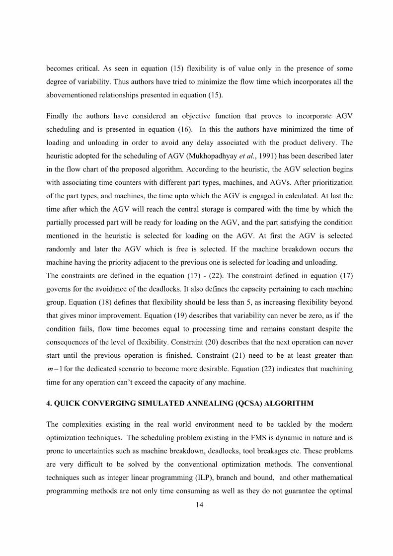


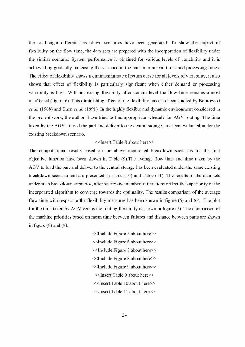


![[inria-00526601, v1] Risk based motion planning and navigation in uncertain dynamic ...emotion.inrialpes.fr/people/spalanzani/Doc/Publication/... · 2011. 10. 19. · uncertain dynamic](https://static.documents.pub/doc/80x56/5fe59019cfc83f2cdc14b30d/inria-00526601-v1-risk-based-motion-planning-and-navigation-in-uncertain-dynamic.jpg)


