Performance Evaluation of Vehicular Ad Hoc Networks using

Performance Evaluation of Vehicular Ad Hoc

Networks using simulation tools

Proyectista: Arvin Rajabi

Directora: Mónica Aguilar Igartua

Co-directora: Carolina Tripp Barba

Barcelona, Julio 2010

Index

3

Index

1. INTRODUCTION and OBJECTIVES..........................................................................21

1.1 Introduction.........................................................................................................21

1.2 Objectives............................................................................................................24

2. HETEROGENEOUS NETWORKS WSN (Wireless Sensor Network) and HSVN

(Hybrid Sensor and Vehicular Network)..............................................................25

2.1 Basics of a HSVN Framework...............................................................................25

2.1.1 Mobility models in VANETs...........................................................................27

2.1.2 Proposal of a communication protocol between WSNs and VANETs.....................28

2.2 Consortia and Sponsorships................................................................................33

2.3 Research studies..................................................................................................37

3. ARCHITECTURE, ROUTING and FORWARDING.........................................................41

3.1 Packet formats....................................................................................................45

3.2 Geographic forwarding.......................................................................................46

3.2.1 Network topology construction.....................................................................46

3.2.2 Packet forwarding strategy...........................................................................46

3.2.3 Query propagation......................................................................................48

3.2.4 Query response..........................................................................................49

3.2.5 Information delivery....................................................................................50

3.3 Mobility management.........................................................................................51

3.4 Load balancing techniques..................................................................................53

3.4.1 Energy-aware forwarding.............................................................................53

3.4.2 Delay-aware forwarding...............................................................................54

Index

4

4. NCTUns 6.0...............................................................................................................57

4.1 Network simulator NCTUns 6.0...........................................................................57

4.1.1 Simulator architecture.................................................................................58

4.1.2 Seamless Integration of Emulation and Simulation............................................59

4.1.3 Support for various important Networks.........................................................59

4.1.4 Support for various Networking Devices..........................................................60

4.1.5 Support for various Network Protocols............................................................61

4.1.6 Software and Hardware System Requirements.................................................62

4.2 Installation of the simulator on Microsoft Windows...........................................63

4.2.1 System Virtual Machine................................................................................63

4.2.2 Dowloading WMware Player.........................................................................64

4.2.3 Dowloading Fedora 11 Virtual Machine with NCTUns 6.0...................................64

4.2.4 Installation steps for Linux............................................................................64

4.2.5 Run the Virtual Machine...............................................................................65

4.2.6 Start using NCTUns 6.0.................................................................................67

4.3 Some screen-shots on NCTUns 6.0......................................................................67

4.3.1 Starting screen............................................................................................67

4.3.2 Topology Editor...........................................................................................68

4.3.3 Attribute Dialog Box.....................................................................................69

4.3.4 Node Editor................................................................................................69

4.3.5 Packet Animation Player...............................................................................70

5. NETWORK and PROTOCOLS...................................................................................73

5.1 Elements.............................................................................................................74

5.1.1 Road segmentation......................................................................................74

5.1.2 Road information data model........................................................................75

5.1.3 Road side sensors........................................................................................76

5.1.4 Mobile car sensors......................................................................................77

5.2 Communication Protocol.....................................................................................78

5.2.1 Static and mobile sensors.............................................................................78

5.2.2 Mobile and mobile sensors...........................................................................79

5.3 Traffic congestion control....................................................................................80

Index

5

6. SIMULATIONS..........................................................................................................81

6.1 Simulation steps..................................................................................................81

6.2 Scenario 1............................................................................................................83

6.2.1 Simulation results........................................................................................83

6.3 Scenario 2............................................................................................................90

6.3.1 Simulation results........................................................................................91

6.4 Problems found during simulations..................................................................105

7. CONCLUSIONS and FUTURE WORK....................................................................107

8. REFERENCES and BIBLIOGRAPHY........................................................................109

6

Figures, Tables and Algorithms Index

7

Figures, Tables and Algorithms index

FIGURES

Fig. 1 - Cooperation between WSN and VANET[ref: Computer communication control inc.

www.cs.nthu.edu.tw/~jungchuk/research.html] ............................................................................................ 22

Fig. 2 - General scenario of a HSVN ................................................................................................................. 27

Fig. 3 - Temporal available time to interchange messages ............................................................................. 32

Fig. 4 - Car 2 Car [ref: www.car-to-car.org] ..................................................................................................... 34

Fig. 5 – CVIS [ref: http://www.cvisproject.org/] .............................................................................................. 35

Fig. 6 – CarLink [ref: http://carlink.lcc.uma.es/] .............................................................................................. 36

Fig. 7 - COMeSafety project [ref: http://www.comesafety.org/] .................................................................... 36

Fig. 8 - System architecture: a mobile sink (MS) querying a WSN while moving. The nodes close to the

streets, called vice-sinks (VSs), are in charge for communicating with MSs. The nodes in the inner WSN,

called sensor nodes (SNs), communicate in a multihop fashion to reach VSs [40]. ....................................... 42

Fig. 9 - An example scenario: cars move around a WSN deployed around a building and look for a free

parking lot [40]. ............................................................................................................................................... 43

Fig. 10 - Example of the considered application scenario. The mobile sink injects a query in the WSN

through the closest vice sink. The query is forwarded to the queried region (highlighted in grey). The

queried data is finally delivered through another VS [40]. ............................................................................. 44

Fig. 11 - A dead lock occurring when forwarding the packet towards a target region and founding a hole:

the scalar product would be maximized by the previous hop, so the back-up mode is entered and the

packet is forwarded around the hole. The back-up angle is reset when a node different from the previsious

hop that maximizes the scalar product towards the destination is found, which happens once the hole is

overcome [40]. ................................................................................................................................................ 48

Fig. 12 - NCTUns 6.0 ......................................................................................................................................... 57

Fig. 13 - Screenshot VMware Player ................................................................................................................ 66


8

Fig. 14 - Screenshot Fedora Log-in .................................................................................................................. 66

Fig. 15 - NCTUns 6.0 starting screen ................................................................................................................ 68

Fig. 16 - The topology editor of NCTUns ......................................................................................................... 68

Fig. 17 - A popped-up dialog box of NCTUns 6.0 ............................................................................................. 69

Fig. 18 - The node editor of NCTUns 6.0 .......................................................................................................... 70

Fig. 19 - The packet animation player of NCTUns 6.0 ..................................................................................... 71

Fig. 20 - System Architecture (52). .................................................................................................................. 73

Fig. 21 – Roadsegmentation [52] ..................................................................................................................... 74

Fig. 22 - Block diagram of road side sensor [52] ............................................................................................. 76

Fig. 23 - Block diagram of mobile sensors [52] ................................................................................................ 77

Fig. 24 - Scenario 1 under evaluation with NCTUns. ....................................................................................... 84

Fig. 25 - Scenario 1: Packet losses evolution for AODV ................................................................................... 87

Fig. 26 – Scenario 1: Packet losses evolution for DSR ..................................................................................... 87

Fig. 27 - Scenario 1: Throughput with AODV and DSR. ................................................................................... 88

Fig. 28 - End-to-end packet delay for AODV .................................................................................................... 89

Fig. 29 - Scenario 1: End-to-end packet delay for DSR .................................................................................... 90

Fig. 30 - Reproduction of the Cerda's idea ...................................................................................................... 91

Fig. 31 - Scenario 2: Percentage of packet losses evolution for AODV and R=100 ......................................... 96

Fig. 32 - Scenario 2: Packet losses evolution for AODV and R=100 ................................................................. 97

Fig. 33 - Scenario 2: AODV throughput with R=100 ........................................................................................ 97

Fig. 34 – Scenario 2: End-to-end packet delay for AODV and R=100 .............................................................. 98

Fig. 35 - Scenario 2: Percentage of packet losses evolution for AODV and R=75 ........................................... 99

Fig. 36 - Scenario 2: Packet losses evolution for AODV and R=75 ................................................................... 99

Fig. 37 - Scenario 2: End-to-end packet delay for AODV and R=75 ............................................................... 100

Fig. 38 - Scenario 2: Percentage of packet losses evolution for DSR and R=100 .......................................... 101

Fig. 39 - Scenario 2: Packet losses evolution for DSR and R=100 .................................................................. 101

Fig. 40 - Scenario 2: DSR throughput with R=100 .......................................................................................... 102


9

Fig. 41 - Scenario 2: End-to-end packet delay for DSR and R=100 ................................................................ 102

Fig. 42 - Scenario 2: Percentage of packet losses evolution for DSR and R=75 ............................................ 103

Fig. 43 - Scenario 2: Packet losses evolution for DSR and R=75 .................................................................... 103

Fig. 44 - Scenario 2: DSR throughput with R=75 ............................................................................................ 104

Fig. 45 - Scenario 2: End-to-end packet delay for DSR and R=75 .................................................................. 104

TABLES

Table 1 - Minimum system requirements ....................................................................................................... 62

Table 2 - *.ptr files fields description .............................................................................................................. 82

Table 3 - Scenario 1: Ratio of time when there is connectivity. ...................................................................... 85

Table 4 - Scenario 1: Simulation settings of the HSVN. ................................................................................... 85

Table 5 - Simulations of Scenario2 .................................................................................................................. 92

Table 6 - Configuration parameters in Scenario 2 ........................................................................................... 93

ALGORITHMS

Algorithm 1 – Example of a query injected in the wireless sensor network by the mobile sink. ................... 49

Algorithm 2 - Packet forwarding strategy ....................................................................................................... 50

Algorithm 3 - Strategy applied at every VS for REPLY packet forwarding when receiving mobility information

......................................................................................................................................................................... 52

Algorithm 4 - awk filter .................................................................................................................................... 95

10

Thanks

11

Thanks

Non ho mai fatto dei ringraziamenti sotto questa forma e forse proprio per questo

motivo provo delle sensazioni strane nel farlo. Ma nonostante ciò è la parte della tesi

a cui tengo di più perchè lo vivo come un resoconto, una tappa, una di quelle

occasioni in cui ci si ferma e si pensa a cosa si è dovuto passare per poter raggiungere

questo traguardo.

Ed è proprio ripensando e andando indietro coi ricordi che mi passano davanti mille

immagini, mille momenti...e naturalmente tutti riguardanti l’ambiente, il luogo, le

persone che mi hanno circondato durante questi anni accademici.

E’ proprio tutto questo che vorrei ringraziare,...gli autori di questi ricordi, le persone

che standomi vicine mi hanno regalato emozioni, esperienze di vita, mi hanno fatto

crescere e sono riuscite a far rimanere vive queste immagini nella mia memoria fino

ad oggi.

Fare un elenco di nomi sarebbe poco elegante e probabilmente riduttivo...sono sicuro

che le persone che stimo, che ammiro e che mi hanno spinto fino a qua, e non solo

durante la mia carriera universitaria, sappiano già che è proprio a loro che rivolgo i

miei ringraziamenti più sinceri.

Ma nonostante ciò mi sento in dovere di fare un’eccezione per le persone che più

amo nella mia vita,...quelle persone che più mi hanno sopportato, che più mi hanno

consigliato, che nonostante li contattassi anche meno di una volta al mese, non

hanno mai smesso di farmi sentire amato anche a 800 km di distanza durante gli

ultimi 2 anni...e che comunque vada nel mio percorso di vita, sono sicuro

continueranno a farlo incondizionatamente...è a voi che dedico questo mio

traguardo, perchè senza di voi non sarebbe mai stato possibile...

Mehdi, Zohreh, Shervin...vi amo.

12

Acronyms

13

Acronyms

AHVN – Advanced Heterogeneous Vehicular Network

AMAC – Adaptive MAC

AODV – Ad hoc On demand Distance Vector

AP – Access Point

BER – Bit Error Rate

C2C – Car-To-Car Communication Consortium

CAS – Content-Addressed Storage

COMeSafety – Co-operative Intelligent Road Transport System

CSM – City Section Mobility

CSMA/CA – Carrier Sense Multiple Access with Collision Avoidance

CSMA/CD – Carrier Sense Multiple Access with Collision Detection

CVIS – Cooperative Vehicular Infrastructure Systems

DSR – Dynamic Source Routing

DTR – Desired Transmission Range

DVB-RCS – Digital Video Broadcasting-Revision Control System

ETSI – European Telecommunications Standards Institute

FTP – File Transfer Protocol

GGSN – Gateway GPRS Service Node

GPRS – General Packet Radio Service

GPS – Global Positioning System

http://encyclopedia.thefreedictionary.com/Carrier+Sense+Multiple+Access+with+Collision+Detection

http://encyclopedia.thefreedictionary.com/Carrier+Sense+Multiple+Access+with+Collision+Detection

Acronyms

14

GUI – Graphical User Interface

HSVN – Hybrid Sensor and Vehicular Network

HTTP - Hypertext Transfer Protocol (world wide web protocol)

ITS – Intelligent Transportation System

JITEL – Jornadas de Ingeniería Telemática

MANET – Mobile Ad Hoc Network

MAS – Mobility-Assist Storage

MDDV – Mobility-centric data dissemination algorithm for vehicular networks

MS – Mobile Sink

NCC – Network Control Center

NCTUns – National Chiao Tung University network simulator

OBU – On Board Unit

OSPF – Open Shortest Path First

PEWASUN – Performance Evaluation of Wireless Ad hoc, Sensor and Ubiquitous Networks

PFC – Projecto Fin de Carrera

PMP – Point to Multi-Point

QoS – Quality of Service

R2C – Road to Car

RACC – Reial Automòbil Club de Catalunya

RCST – Return Channel Satellite Terminal

RSU – Road Side Unit

RTP – Real Time Protocol

SGSN – Serving GPRS Service Node

SN – Sensor Node

SSM – Stop Sign Model

TCP/IP – Transmission Control Protocol / Internet Protocol

TSM – Traffic Sign Model

TTL – Time to Live

http://www.thefreedictionary.com/Hypertext+Transfer+Protocol

http://encyclopedia2.thefreedictionary.com/Open+Shortest+Path+First

Acronyms

15

UDP – User Datagram Protocol

V2I – Vehicle to Infrastructure

V2V – Vehicle to Vehicle

VANET – Vehicular Ad Hoc Network

VADD – Vehicle-assisted data delivery in vehicular ad-hoc networks

VS – Vice Sinks

WSN – wireless sensor network

16

Summary

17

Summary

Recent studies demonstrate that the routing protocol performances in vehicular networks can

improve using dynamic information on the traffic conditions. WSNs (Wireless Sensor

Networks) and VANETs (Vehicular Ad Hoc Networks) are exactly related with this statement

and represent the trend of wireless networks research program in the last years.

In this context, a new type of network has been developed: in fact, HSVN (Hybrid Sensor and

Vehicular Network) let WSNs and VANETs cooperate through dynamic information data

exchanges with the aim to improve road safety, and especially to warn the driver and the co-

pilot of any event occurred in the road ahead, such as traffic jam, accidents or bad weather.

The results will be immediate: less accidents means more saved lives, less traffic means a

pollution decrease, and from the technological point of view, this communication protocol will

open the door to attractive services, such as downloading of multimedia services or internet

browsing, that means easier, safer and more comfortable trips.

It is out of doubt that speaking about cars and road technology developments, the market

and the interests about this field increase exponentially. Recent projects such as CVIS [1]

and COMeSafety [2], focused on improving the road driving, and are the concrete

demonstration that this entire context can get soon very close to reality.

Owing to their peculiar characteristics, VANETs require the definition of specific networking

techniques, whose feasibility and performance are usually tested by means of simulation.

Starting from this point, this project will present a HSVN platform, and will also introduce and

evaluate a communication protocol between VANETs and WSNs using the NCTUns 6.0 [3]

simulator. We will particularly analyze the performances of 2 types of Scenarios developed

during our project. Both of them are in an urban context, but we will extract different useful

results analyzing the packet losses, the throughput and the end-to-end packet delay.

18

Resumen

19

Resumen

Estudios recientes han demostrado que el desempeño de los protocolos de encaminamiento

en redes vehiculares puede mejorarse mediante la utilización de información dinámica sobre

las condiciones de tráfico. Las redes de sensores (WSNs, Wireless Sensor Networks) y las

redes vehiculares (VANETs, Vehicular Ad Hoc Networks) están directamente relacionadas

con estos estudios y representan una tendencia de investigación en el campo de redes

inalámbricas en estos últimos años.

En esto contexto, se ha desarrollado un nuevo tipo de red, una red hibrida vehicular y de

sensores (HSVN, Hybrid Sensor Vehicular Network) que permite la cooperación entre

WSNs y VANETs a través un intercambio dinámico de información con el fin de aumentar la

seguridad vial, y en particular advertir el conductor y el copiloto de cualquier tipo de evento

que pueda pasar en su trayecto, como congestión de tráfico, accidentes o datos

meteorológicos que dañen el estado de la carretera. Esto dará como resultado inminente:

menos accidentes lo cual supondría salvar vidas humanas, menos trafico que ayudaría a

disminuir la contaminación y desde el punto de vista tecnológico, este tipo de comunicación

abrirá las puertas a otros servicios atractivos como la descarga multimedia de servicios o el

navegar en internet, lo cual permite seguridad y confort en los viajes por carretera.

Sin duda alguna, al hablar de coches y de desarrollo de tecnologías vial, el mercado y los

intereses sobre estos campos aumenta exponencialmente. Proyectos recientes como CVIS

[1] y COMeSafety [2] se concentran en mejorar la conducción vial, y son la clara muestra

que todo este contexto puede llegar pronto muy cerca a la realidad.

Debido a sus características específicas, una VANETs requiere la definición de técnicas de

red específicas, cuya confiabilidad y rendimiento son por lo general probados con

simulaciones. Empezando desde este punto, esto proyecto presenta una plataforma HSVN,

y también introduce y evalúa la comunicación entre VANETs y WSNs usando el simulador

NCTUns 6.0 [3]. En particular analizamos el rendimiento de dos escenarios, uno

desarrollado durante el proyecto en contraste con otro propuesto en [60]. Ambos son en un

entorno urbano, pero alcanzamos diferentes resultados útiles analizando las pérdidas de

paquetes, el throughput y el retardo extremo a extremo de los paquetes.

20

Chapter 1. Introduction and objectives

21

Chapter 1. Introduction and Objectives

1.1 Introduction

During the last few years, continuous progresses in wireless communications

have opened new research fields in computer networking, aimed at extending

data networks connectivity to environments where wired solutions are

impracticable. In this work we will focus more our attention on short range

technologies: ad hoc networks, because of the easy deployment it requires,

have become one the most followed network technology. An ad hoc network [4]

is formed by a group of nodes that communicate with each other by wireless

interfaces, either with a fixed infrastructure or without any kind of infrastructure.

These are the dynamic properties we will found analyzing this two kind of ad

hoc networks: WSNs (Wireless Sensor Network) [5] and VANETs (Vehicular Ad

Hoc Networks) [6] [7].

Both WSNs and VANETs are ad hoc networks which can operate without any

infrastructure or centralized management. In such a case, the network

organization is carried out by the nodes themselves. Every node is capable to

work as a sender, destination or as a forwarding node. Nodes in WSNs are

static, while nodes in VANETs can achieve very high speeds. This motion of the

nodes produces frequent changes in network topology, so that the design of

routing protocols able to adapt to the dynamic environment is a really

challenging task (Fig.1).


22

Fig. 1 - Cooperation between WSN and VANET[ref: Computer communication control

inc. www.cs.nthu.edu.tw/~jungchuk/research.html]

WSNs consist of a small group of wireless devices able to gather information

from their environment, such as temperature, humidity, movement, etc. It is

typically constituted by: a set of resource-constrained nodes, which are

deployed over the spatial region to be observed and capable of performing

user-defined tasks related to data gathering and one (or multiple) sink

node(s), where information gathered by the WSN can be accessed by the end-

user. Often WSNs are deployed in remote and/or hostile regions, and the sink

is the only node through which the WSN is first queried and then accessed

for data gathering operations. Hence, the sink is expected to be

connected to the backend through some form of long-range connection (i.e.,

satellite communication, Wi-Fi, WI-Max, etc.). This type of network allows fast

deployment of their devices due to their small size and weight. Nonetheless, it

has some restrictions in comparison to other ad hoc networks, such as their

limited memory, scarce energy, small transmission range and low processing

capacity.

In ITS (Intelligent Transportation System), this may result extremely inefficient

in terms of infrastructure to be deployed, and management overhead in order

to guarantee the correct operations of the network. In fact, when considering

an urban setting, the scenario differs significantly from the previous one.

Indeed, let us assume the WSN to be deployed along a road, or in city area


23

covered by a specific pervasive service. Let us further assume the end-user,

while moving around the city, to be in direct contact with the WSN, thus acting

both as end-user and sink at the same time. In this case, the mobile user can

directly access services offered by the ubiquitous WSN, without the need to

resort to a remote repository where data is first stored, and then accessed.

This is the case of ITS, where deployed WSNs enable cars to obtain

information on the conditions of the surrounding environment, and to use this

information for taking appropriate decisions. The WSN could be for

instance used for detecting the formation of ice over the road, or monitoring

the status of parking spots along the streets of the city center.

A VANET can be considered as a particular type of MANET (Mobile Ad hoc

Network) [4]. However, the main difference is the speed in nodes. This factor

may produce quick changes in the network topology and thus turn out to short

link lifetimes. In addition, vehicle's devices hardly have limitations regarding

energy supply and can have a high processing power. By the end of 2010, the

standard IEEE 802.11p [8] [9] is expected to be released, and it will contribute

to improve communication among vehicles and also between vehicles and RSU

(Road Side Units). Also, vehicles are envisioned to carry multiple types of

wireless transceivers to be able to communicate across more than one wireless

data links; vehicles will be equipped with an OBU (On-Board Unit) which will

manage the communication between different technologies (e.g. 2G/3G,

WiMax, satellite). Besides, vehicles will easily get Internet connectivity through

the closest available AP (Access Point) along the roadside.

A new approach has recently been proposed which merges both WSN and

VANET networks. HSVNs (Hybrid Sensor and Vehicular Networks) consist in

making WSNs and VANETs work jointly to constitute a communication

framework to be used by vehicles in order to assist drivers to reduce road

accidents, fatalities and injuries. Recently, new architectures have been

proposed to offer robust, reliable and cost-effective approaches for HVSNs.

HSVNs are introduced as a new concept of road sensor deployment, and they

can be seen as a new kind of new generation network architecture. In a global

perspective, weather events conditions, such as rain or ice, or the amount of

traffic density in remote road segments can be monitorized by the cars. All the

road information gathered by the cars will be stored in WSNs, wich are

deployed along the roadside, to be later spread among other passing vehicles.

This way, VANETs enlarge their scope, since other passing vehicles can

recover that information later. The purpose of HSVNs is that vehicles within the

VANET can share information regarding climate conditions, traffic state and

road safety, seeking to reduce the number of accidents. Thanks to this

information interchange, users might drive safer along the routes.


24

1.2 Objectives

The main objectives of our project can be classified as follows:

Study the protocols: MAC, Network Routing (DSR,AODV), ...

Design several representative scenarios for VANETs: city, rural, highway.

Decide the proper configuration settings to model these scenarios in real

life: speeds, network nodes, size, number of vehicles, number of lines,

measurements, transmission range, ...

Implement the scenarios in NCTUns 6.0

Performance evaluation, analysis of results, conclusions.

Work in conjuction with a PhD student, Carolina Tripp Barba [ref:

http://sertel.upc.es/~ctripp] in her research work during the thesis

http://sertel.upc.es/~ctripp

Chapter 2. Heterogeneous Networks WSN and HSVN

25

Chapter 2. Heterogeneous Networks WSN

and HSVN

2.1 Basics of a HSVN Framework

In this chapter we summarize the HSVN (Hybrid Sensor and Vehicular Network)

platform designed by Carolina Tripp Barba [ref: http://sertel.upc.es/~ctripp ]in her

PhD research work. The proposal has been published in the Spanish Conference

JITEL (Jornadas de Ingeniería Telemática) 2010 and is currently accepted from

the international conference PEWASUN (Performance Evaluation of Wireless Ad

hoc, Sensor and Ubiquitous Networks) and it will be presented on october 2010.

The main feature offered by vehicular networks is the capability to distribute

traffic road information among the vehicles of a road. Nodes in vehicular

networks will be able to access to different information related to their

environment. This information can be useful to assist data routing protocols in

VANETs to make proper decisions, e.g. detect those vehicles with similar routes

to compose routing paths seeking to increase path lifetimes. The flooding

mechanism is not very functional because of the potential high number of nodes

in a VANET; instead, the multihop network feature is used, which allows

spreading information vehicle by vehicle until the destination node is reached, in

case sender and destination are not in the same transmission range. A

dissemination protocol to distribute road data through the VANET is required.

Public transportation may also be involved in the communication network. Buses

can operate as reliable VANET nodes and also to offer Internet connection to

other passing vehicles. In VANETs, it is typically assumed that each node in the

network is equipped with some navigation system and also with a GPS (Global

Positioning System) [10]. Nowadays, most of the modern cars already have a

GPS installed, so that car navigation systems (e.g. Tom-Tom [11], GARMIN [12])

are able to know their geographical position and to obtain digital maps as well.

This information can be useful for the car navigation system to make proper

http://sertel.upc.es/~ctripp


26

decisions, for example to take the most reliable and safer non-congested road

from several options.

A simple, fast and efficient communication protocol has to be designed to allow

communication between VANETs and WSNs. Both networks must share data

that carry road information and short video streams. The data interchange has to

be produced very fast, since the interval in which the vehicle is under the

transmission range of the WSNs is very short. The cooperation between WSNs

and VANETs makes it possible to extend the transmission range in a VANET to a

larger region with the cooperation among ad hoc nodes within both networks.

Vehicles can store road information in the WSN‟s sink as they pass through that

WSN. Later on, other passing cars can recover that information from the WSN's

sink, as it can be seen from Fig. 2.

The content of the interchanged messages regarding road safety has to be

defined. Messages have to include information (e.g. weather conditions, location

of accidents, possible building work, etc) about different road segments.

Messages can include a low quality image of the incoming intersections, so that

the co-pilot or the driver could have a quick look to foresee actual information of

the road ahead. After that, the data interchanged between the WSN's gateway

and the vehicle in the VANET, will be stored or updated at their respective data

bases. Moreover, the protocol to be designed has to manage other kind of data

interchange (see Fig. 2) which is described as follows:

Group leader vehicles (cars A and C in Fig. 2) gather road information

from the vehicles behind in their respective groups.

The road information is interchanged between group leaders which

travel in opposite directions (cars A and C in Fig. 2).

The new received information is spread from the group leader among

the vehicles in the group.

Passengers can access to the Internet by means of the APs spread

along the roadside or also by means of public transportation with

Internet connection.


27

Fig. 2 - General scenario of a HSVN

2.1.1 Mobility models in VANETs

In a vehicular scenario, cars do not move freely throughout the whole area.

Instead, they follow the lanes of the road or the streets in a city, they follow

traffic signals and they are aware of the other vehicles. In addition, the

node‟s distribution is not constant; on the contrary vehicles tend to create

groups. The type of road must also be considered because most of the

parameters (number of lanes, speed of the nodes, etc.) change from one

scenario to another (rural, motorway, urban). In order to achieve realistic

results, all these features have to be taken into account when designing a

HSVN framework.

A mobility model describes the movement pattern followed by the nodes in a

specific scenario. Those mobility models need to be included in the

simulations carried out to analyse the performance evaluation of new routing

and communication protocols designed for HSVNs. Choosing the proper

simulation settings and mobility model is crucial since these configuration

parameters will determine the results. For instance, in an urban scenario it is

very important to include obstacles, roads, traffic lights and signals. Some


28

research works, such as [13], show how important it is to consider a realistic

mobility model for VANETs to obtain reliable simulated results close to real

scenarios. In that work, [13], the authors carried out several simulations with

several models like Freeway [14], Manhattan [14], CSM (City Section

Mobility) [15], SSM (Stop Sign Model) [16], TSM (Traffic Sign Model) [16],

STRAW [17], etc. They conclude that the first three are inappropriate for

simulating VANETs, whereas the last three ones are more realistic, as they

involve traffic lights and stops signs.

2.1.2 Proposal of a communication protocol between

WSNs and VANETs

In the following, we describe the communication algorithm between WSNs

and VANETs that we have designed. The main purpose is to fulfil all the

types of communications produced between vehicles and static road

sensors.

There are 3 types of communications to be considered between WSNs and

VANETs, which are depicted in Fig. 2:

a) Communications between static sensors in a WSN and vehicles in a

VANET

WSN --> Vehicle

a.1. The WSN's gateway detects a vehicle within its transmission

range.

a.2. The WSN's gateway sends a connection request (14 bytes)

to the passing vehicle.

Vehicle --> WSN

a.3. The vehicle sends back an ACK (14 bytes) to the WSN's

gateway. This ACK contains the coordinates of its destination (20

bits). This way the vehicle sets high priority to the information of

its own interest. It also includes the ID (identification, 20 bits) of

the vehicle.


29

WSN --> Vehicle

a.4. Transmission of a packet including road information

regarding all segments that are in the path along the destination

of the passing vehicle. Also, data regarding other paths. The

packet contains this information:

_ a.4.1. A two-bits header field per road segment that includes

information about the state of the traffic density of each road

segment along the path. The data codification is: 0=free

segment, 1=semi-congested segment, 2=very congested

segment, n/i=unknown information.

_a.4.2. A two-bits header field per road segment that includes

information about the weather/accident state of the roads. The

data codification is: 0=good weather conditions, 1=ice, 2=rain,

3=accident.

a.5. Transmission of a small image (50 Kbytes approx.)

regarding the next cross of the path in the vehicles‟ destination.

After that, other images regarding other intersections can be

sent, as long as both nodes are in transmission range.

Vehicle --> WSN

a.6. The vehicle sends to the WSN's gateway road information

(data and image) which was previously gathered from other

vehicles or other WSN. The WSN updates that information (if

newer) regarding the state of the roads. The content and

codification of the packets that include this road information, is as

described in a.4.

Vehicle --> WSN

a.7. The vehicle reaches the coverage limit and the connection

ends.

b) Vehicle-to-Vehicle communications. Vehicles move in the same direction

Vehicle A --> Vehicle B

b.1. Vehicle B is detected by vehicle A within its transmission

range. Vehicle B is behind vehicle A in the same direction (see

Fig. 2).


30

b.2. A connection request (14 bytes) is sent by vehicle A to

vehicle B.

Vehicle B --> Vehicle A

b.3. An ACK (14 bytes) is sent by vehicle B to vehicle A. It

includes its ID (identification, 20 bits). It also includes its

destination coordinates.


b.4. Data transmission regarding the state of the roads and traffic

density of all the road segments that are in the destination path

of vehicle B and also of the roads within other paths. The packet

contains this information:

_ b.4.1 A two-bits header field per road segment that includes

information about the state of the traffic density of the road

segment. The data codification is: 0=free segment, 1=semi-

congested segment, 2=very congested segment, n/i=unknown

information.

_ b.4.2 A two-bits header field per road segment that includes

information about the weather/accident state of the roads. The

data codification is: 0=good weather conditions, 1=ice, 2=rain,

3=accident.

b.5. Transmission of a small image (50 Kbytes approx.)

regarding the next cross of the path in the destination of vehicle

B. After that, other images regarding other intersections can be

sent, as long as both nodes are in transmission range.


b.6 Vehicle A reaches the coverage limit of vehicle B and the

connection ends.

In this way, the road information is spread backward through the group

of vehicles. In addition, every new incoming vehicle in the group sends

its own new road information forward till the leader, through the other

relying vehicles in the group. This way, the leader gathers the whole

road information of its group of vehicles.


31

c) Vehicle-to-Vehicle communications. Vehicles move in opposite direction

Vehicle A in one direction --> Vehicle C in the opposite

direction (see Fig. 2).

c.1. In case that the detected vehicle goes in opposite direction,

the connection will only be established between the first vehicles

of both groups (group leaders). The communication between

vehicle A and vehicle C is as described in b) from b.1 to b.6.

c.2. Each group leader disseminates the new road information

among the vehicles within its own group.

Regarding the amount of information needed to communicate the state of

the whole road segments that belong to a destination let us make some

considerations. There may be a different number of road segments per

destination. Basically, it depends on the type of scenario (urban, rural,

motorway) and on the total road length to that destination. For example, in

case of a motorway with a total 500 km of an average long trip and road

segments (located between exits) of 10 km each, there would be about 50

segments in such a trip. In case of a rural road with an average 50 km trip

and road segments of 5 km, there would be around 10 road segments.

Finally, in city scenarios where typical trips take around 5 km and road

segments measure about 200 m, there are around 25 segments per

average trip. Next list summarizes the number of road segments per typical

trip in each scenario.

In a motorway, 50 road segments, 500 km trip

In rural road, 10 road segments, 50 km trip

In city, for 25 road segments, 5 km trip

In order to estimate if there is enough time to fulfil the data interchange

between the WSN sink and a passing vehicle, let us see a numerical

example.

The IEEE 802.11b MAC has a nominal link bandwidth of 11Mbps and a

throughput around th=7Mbps (for UDP like traffic). We consider a maximum

speed of the vehicle of v km/h and a transmission range of the WSN sink

node of r m. Then, the available time for the data interchange is tavailable ≈

2r/v sec, as depicted in Fig. 3. During this time the communication is

established and the transmission of all the packets must be done,


32

according to the messages interchange described in point a) of the

communication protocol.

Fig. 3 - Temporal available time to interchange messages

The data information regarding all the road segments is transmitted in a

single packet of size p=1000 bytes, which takes troad_segments=p/th=1,14 ms.

The transmission of an image of 50 Kbytes takes 50 packets and

timage=0,057 sec. The total time required to send that information is trequired

=troad_segments+timage=0,058 sec. Thus, if trequired < tavailable the exchange of

information (data and images) between the car and the sensor sink can be

successfully done. Furthermore, more images regarding other intersections

could be sent as well within the available interval of time, tavailable.

Let us consider a transmission range of the sink WSN node of r=80 m. Let

us estimate the tavailable=2r/v values for each type of scenario.

In a motorway, for v=120 km/h, tavailable = 4,8 sec

In a rural road, for v=80 km/h, tavailable = 7,2 sec

In a city, for v=50 km/h, tavailable = 11,52 sec

We can see that trequired = 0,058 sec. << tavailable in every scenario, so that

more additional images (timage=0,057 sec) could be sent during the available

period of time.


33

2.2 Consortia and Sponsorships

Recently, different consortiums have been created in Europe which aim to make

safer vehicles and roads. These consortiums are mainly integrated by car

manufacturers, researchers and the European Commission. Among other

projects, we highlight the following.

The CAR 2 CAR [18] communication consortium is a non-profit industrial driven

organization initiated by European vehicle manufacturers supported by

equipment suppliers, research organizations and other partners. Their objective

is to increase road safety and driving efficiency by means of cooperative

intelligent transportation systems (ITS), vehicle to vehicle (V2V) and vehicle to

infrastructure (V2I) communications. As we can find on their web-site “www.car-

to-car.org”, the main objectives can be resumed in this steps:

the development and release of an open European standard for

cooperative Intelligent Transport Systems and associated validation

process with focus on Inter-Vehicle Communication Systems.

to be a key contributor to the development of a European standard and

associated validation process for Vehicle-2-Roadside Infrastructure

Communication being interoperable with the specified inter-vehicle

communication standard.

to provide its specifications and contributions to the standardisation

organisations including in particular ETSI TC ITS in order to achieve

common European standards for ITS.

to push the harmonisation of Car-2-Car Communication Standards

worldwide.

to promote the allocation of a royalty free European wide exclusive

frequency band for Car-2-Car Applications.

to develop realistic deployment strategies and business models to

speed-up the market penetration.

to demonstrate the Car-2-Car System as proof of technical and

commercial feasibility.


34

Fig. 4 - Car 2 Car [ref: www.car-to-car.org]

The CVIS (Cooperative Vehicle-Infrastructure Systems) [1] project deals with

intelligent co-operative systems that are based on V2V and V2I communications

to achieve improvements both in the efficiency of the transport systems and in

the safety of all road users. The expected benefits stem from the increased

information that is available of the vehicle and its environment. Those benefits

include an increase in road network capacity, reduction of congestion and

pollution, shorter and more predictable journey times, improved traffic safety for

all road users, more efficient logistics, improved management and control of the

road network (both urban and inter-urban), increased efficiency of the public

transport systems and better and more efficient response to hazards, incidents

and accidents.


35

Fig. 5 – CVIS [ref: http://www.cvisproject.org/]

CARLINK [19] seeks to develop intelligent service platforms for vehicles. The

primary application of this project is to offer real time local weather information,

transit reports and other broadcast applications. Vehicles are equipped with

transceivers that are able to communicate with base stations and with other

nodes of the ad hoc network. The goals of this project aim at improving car

industry, telecommunication operators, private drivers, public transportation,

truck traffic and other road users. New cars are foreseen to include new safety

features and new kind of telecommunication services related to ITS, which will

bring new kind of business opportunities to telecommunication operators.

http://www.cvisproject.org/


36

Fig. 6 – CarLink [ref: http://carlink.lcc.uma.es/]

The COMeSafety project [2] supports the eSafety Forum [20] with respect to all

issues related to vehicle-to-vehicle and vehicle-to-infrastructure communications

as the basis for cooperative intelligent road transport systems. Also, it provides

an open integrating platform, aiming at the interests of all public and private road

safety stakeholders to be represented. Consolidated results and interests are

submitted to the European and worldwide standardization bodies (Fig.7).

Fig. 7 - COMeSafety project [ref: http://www.comesafety.org/]

http://carlink.lcc.uma.es/

http://www.comesafety.org/


37

INFOTRANSIT [21] has been developed by the RACC (Reial Automòbil Club de

Catalunya) foundation which provides data to make a safer road. It consists in an

Internet service based on different data sources that provide real time traffic,

weather information, speed cameras location, traffic congestion, and accident

location. Its interactive map is based on Google maps [22]. In the near future,

drivers are expected to easily access to updated traffic information every moment

during the trip in a cost-free fashion using the infrastructure along the roadside,

e.g. RSUs. This traffic information will be provided by the Traffic Management

Unit of each country. Drivers will easily be able to see the location of speed

radars, short video streams from traffic cameras, or the location of any incident

occurred in the roads.

2.3 Research studies

Regarding HSVNs, several research studies have been made whose principal

challenges are the architecture design. HSVNs need to include a reliable

communication protocol between VANETs and WSNs, which have to interchange

dynamic and static data from their respective nodes. Most of the studies make

several assumptions such as GPS devices available in all vehicles, embedded

microprocessor and sensors in the road side devices, and the use of identical

digital maps in the whole network. One of the most important features is that

there is no limit in the batteries lifetime of the road side devices or in the storage

size as well.

Some research results in network devices and sensors nodes for this kind of

networks are proposed in “A Collaboration-based Hybrid Vehicular Sensor

Network Architecture” [23] where the tasks of the mobile sensors, the traffic

control in the system, the content of the shared information and the

communication protocols are described.

Another study “A secure and Resilient WSN Roadside Architecture for Intelligent

Transport System” [24] focused on providing a safer road presents a cost-

effective road-to-car (R2C) approach based on WSNs. It is based on the

implementation of several sensor devices along the road, which is divided into

road segments. An island of sensors will gather information about the weather

status as well as other information from the vehicles. This study gives a new

approach which can be used in two different services: accident prevention and

post-accident investigation. Such information can be used to save lives and also

to be used by the forensic teams as a reliable source of the facts.


38

Also, “Vehicular telematics over heterogeneous wireless networks: A survey.

Computer Communications” [25] presents the benefit of using multiple access

technologies and multiple radios in a collaborative manner, to create an

advanced heterogeneous vehicular network (AHVN) architecture.

Car Tel [26], deployed on 6 cars, is a mobile sensor computing system designed

to collect, process, deliver, and even visualize data from sensors located on

mobile unites. It can provide a simple query-oriented programming interface,

handle large amounts of heterogeneous data from sensors, and handle

intermittent and variable network connectivity.

Mob Eyes [27], an efficient lightweight support for proactive urban monitoring by

exploiting vehicle mobility to opportunistically diffuse summaries about sensed

data. Mobi Eyes can harvest summaries and build a low cost distributed index

with reasonable completeness, good scalability and limited overhead.

The performance of 802.11b in vehicular sensor networks has been examined by

many papers. The authors of “Drive throu internet: IEEE 802.11b for automobile

users” [28] have shown how long a connection can be maintained between a

moving car and a road side sensor while driving at different speeds between 80-

180km/hour. They show the communication could be kept for 4-9 seconds and

about a third of the connection can be reasonably used. Furthermore, at speeds

of 80km/hour, up to 9MB of data can be transmitted.

More recently in “A measurement study of vehicular internet access” [29], a

measurement study, which was performed more than 290 hours over 9 cars,

shows that the median duration of link-layer connectivity at vehicular speed is 13

seconds, the median connection upload bandwidth is 30KByte/s and that the

meanduration between successful associations to road side access points is 75

seconds.

And in “Vehicular opportunistic communication under microscope” [30] the

authors show that only 50% of the overall possible throughput is achieved with

current protocol, quantify the effects of ten problems caused by theexsting

protocol and recommend best practices for using vehicular opportunistic

connections. They also show that if the environmental information is available to

the 802.11 MAC and to TCP, the overall throughput could be significantly

improved.

Based on the use of opportunistic sensor networking approach, Metro Sense [31]

is able to scale to very large areas. Opportunistic sensor networking provides

mobility-enabled interaction and coordination between people-centric mobile

sensors, static sensors and access points in supportof opportunistic sensing,

opportunistic tasking, and opportunistic data collection.

Due to the nodes‟mobility, vehicular sensornetworks displays intermittent and

variable network connectivity. Ice DB [32], a continuous query processing system


39

for intermittently connected mobile sensor networks has been developed. The

delay-tolerant query processor is coordinated by a central server and mobile

nodes. And the algorithm to prioritize query results improves the application

defined metrics.

In the aspect of data storage, “Efficient data harvesting in mobile sensor platform”

[33] proposes two architectures, Content-Addressed Storage (CAS) and Mobility-

Assist Storage (MAS). While CAS utilizes info stations by hashing the key of an

event to a specific info station, MAS opportunistically disseminates events by

”relaying” or sending events only to one‟s neighbors.

To disseminate data to a certain destination, MDDV (Mobility-centric data

dissemination algorithm for vehicular networks) [34] combines the idea of

opportunistic forwarding trajectory based forwarding and geographical

forwarding. And VADD (Vehicle-assisted data delivery in vehicular ad-hoc

networks) [35] makes use of the existing traffic pattern to forward the packets to

the best road with the lowest data delivery delay. Similarly, based on the location

information, “Location-aware services over vehicular ad-hoc networks using car-

to-car communication” [36] introduces a location-aware, application-layer,

communication protocol designed to support a distributed service infrastructure

over vehicular sensor networks.

To identify the street traffic conditions, an algorithm proposed by “Surface street

traffic estimation” [37] is simple but effective. Based on road segmentation, it only

needs GPS location data and in frequent low-bandwidth cellular updates to plot a

spatio-temporal traffic plot converted from cumulative time-location plots, then

classify the past data to estimate the road condition.

40

Chapter 3. Architecture, Routing and Forwarding

41

Chapter 3. Architecture, Routing and

Forwarding

This application domain, while intuitively clear, requires a general refinement of the

standard WSN architecture and protocols. In particular, we are moving from a

centralized architecture, where nodes self-organize at bootstrap phase for the delivery of

data to the sink node, to a fully distributed one, where no pre-determined gateway can be

identified.

Furthermore, mobility management strategies and geographic forwarding stress a

particular subset of the nodes in the network and expose them to energy failure. In order

to prolong network life time, we summarize here an energy-aware forwarding strategy and

a delay-aware forwarding strategy *.

In these strategies, nodes take decision on the next hop not only on the basis of geographic

information, but also on the energy consumed by the neighbour or on the delay expected

when sending a packet towards another node. In order to do that, the metric considered in

simple geographic forwarding (i.e., a scalar product among the target direction and the

neighbour direction) is weighted by the consumed energy in energy-aware forwarding and

with the delay in delay-aware forwarding. In such a way the more stressed nodes are

avoided from a certain point on and the performance is improved.

The operative scenario the authors refer to in [38] [39] is constituted by an information

retrieval area, where nodes sensing a phenomenon of interest are deployed, with one

or more mobile users moving around it and querying for data. As an example, this

includes the case of cars moving around at rush hours, and looking for a free parking

spot in a particular area (i.e., close to a subway station, close to user‟s favorite shop). To

this purpose a car acts as a sink: along its trajectory it gets temporarily connected to the

network, it sends a query asking for information on certain geographical region, and then

waits for the corresponding data.

(*): In this chapter, part of the work appeared in the Proc. of IEEE ICC 2007 [38] and in Proc. of IEEE Globecom 2007

[39]. The work of D.Miorandi and I.Carreras has been partially supported by the EC within the framework of the BIONETS

project EU-IST-FET-SAC-FP6-027748 (http://www.bionets.eu).


42

In the aforementioned scenario we can identify three different roles, as shown in Fig.8:

Sensor nodes (SNs), in charge of „„sensing” a certain zone. We assume a large

number of SNs to be deployed around a building in a block of a city town or in a

trading center, detecting a parking lot around the building to be free or occupied.

Furthermore, we assume each SN to be aware of its geographical position, for instance

by storing in each node its coordinates during deployment. Alternatively, a

distributed localization scheme can be used, where network nodes cooperate in order to

reconstruct their spatial distribution.

Vice sinks (VSs) that constitute the edge nodes managing the communications from

and to MSs. We assume each VS to be aware of its position and of the position of the

closest VSs and to have a unique progressive identifier (ID).

Mobile sinks (MSs), comprising the nodes moving along the deployment

area where the VSs are deployed. We assume each MS to be equipped with a

satellite receiver like GPS, so that information on position, direction and speed is

always available.

Fig. 8 - System architecture: a mobile sink (MS) querying a WSN while

moving. The nodes close to the streets, called vice-sinks (VSs), are in charge

for communicating with MSs. The nodes in the inner WSN, called sensor

nodes (SNs), communicate in a multihop fashion to reach VSs [40].

VSs are disseminated along the WSN network perimeter, but no particular

constraint is applied to their density. In particular, it is not assumed that the MS is

always reachable, thus resulting in several disconnections experienced from the

MS, and it is not assumed that the VSs form a subnetwork, as they are not


43

necessarily connected to each other. MSs are assumed to move according to a

constrained random way point mobility model, where their position is constrained

to stay along the peripheral area inside which the WSN is deployed. This includes

the case of mobile users driving around a city block, and looking for a free parking

spot as depicted in Fig.9. The communication architecture needs to be designed in

such a way that a MS is allowed to send a query and to receive related responses,

managing in a transparent way possible disconnections. It implies defining proper

interfaces among MS, VSs and SNs.

Fig. 9 - An example scenario: cars move around a WSN deployed around a building and

look for a free parking lot [40].

The routing framework proposed in [40] for the outlined architecture is based up

on a geographic routing forwarding strategy enhanced with mobility prediction. In

fact, after a query is injected in the network by a MS, a response message is

expected to reach the outer nodes of the network by predicting the new position of

MS, according to the mobility information included in the original query message.

Typically, the VS node closest to the estimated position will be reached by the

response packet. Then, if the MS is effectively in local proximity of the VS , the

response is delivered with success, otherwise the packet needs to be routed

towards the most likely actual positionof the MS. In order to support that, the

authors in [40] proposed a geographic forwarding strategy coupled with an efficient


44

mobility prediction scheme, able to use, at the VSs, the latest mobility information

available at the MS.

Fig. 10 - Example of the considered application scenario. The mobile sink injects a query in the

WSN through the closest vice sink. The query is forwarded to the queried region (highlighted in

grey). The queried data is finally delivered through another VS [40].

The reference scenario is summarized in Fig.10, where the MS injects a query in

the WSN through the first VS. The query is then forwarded to the interested region

(highlighted in grey) where the destination node(the closest to the center of the

region) aggregates data of the region of interest by querying other nodes

belonging to the same region. The aggregated data is then sent towards the target

destination. The requested information is first forwarded from the SNs by means of

multihop communications, and, finally, delivered from the last VS to the mobile

sink.


45

3.1 Packet formats

Before going into details of the routing strategy, I will introduce five different types of packets needed in order to support both the geographic forwarding and the mobility prediction strategies. The packets, their fields and the actors in the network managing them are the followings:

HELLO packet: a simple packet sent periodically containing node‟s ID, geographical position, a flag to specify whether it is a VS node or not, the remaining energy (used for energy-aware forwarding) and the current duty cycle (used for delay-aware forwarding).

MOBILITY packet: a simple packet sent by the MS to every VS in local proximity, containing direction of movement, geographic coordinates, speed and a global time stamp.

ALERT packet: a message generated by every VS upon notification by a MS of a change occurred in its mobility pattern. It contains all the informatio contained also in the MOBILITY packet, plus the ID of the originating VS, the network address of the sender of the packet and the geographical coordinates of the destination of the ALERT packet.

QUERY packet: a message generated by the MS after selecting the target region of the query itself. It contains the mobility information as in the MOBILITY packet, the geographical coordinates of the center of the target region and its radius of interest, the network address of the sender and the TTL of the packet.

REPLY packet: a message generated by the SN closest to the center of the target region of the QUERY packet that contains all the mobility information of the originating MS as in the MOBILITY packet (copied from the QUERY packet), the actual position of the MS evaluated hop by hop according to mobility information and elapsed time, the network address of the sender and the TTL of the packet (copied from the QUERY packet).

The way these packets are handled by the routing framework is described in the following subsections.


46

3.2 Geographic forwarding

As stated at the beginning of the chapter, we assume each node of the

network to be aware of its position and each MS to be enabled with a

satellite receiver such that it is able to know its coordinates, speed,

direction and global time-stamp. For the sake of simplicity, let us identify

the coordinates of the target region stored in the QUERY packet with

TargetPos, the coordinates of the MS stored in the REPLY packet with

MsPos and the coordinates of the node that is currently taking the

decision on the next hop with CurrentPos.

We describe the routing framework by separating the phases shown in

the following.

3.2.1 Network topology construction

In the network bootstrap phase each SN builds its onehop

neighbour table by means of reciprocal HELLO packets exchange.

Every node at bootstrap sends a HELLO packet described in

Section 3.1. HELLO messages are scheduled at random instants in

order to avoid collisions. Once the bootstrap phase is over, every

node has created a routing table containing neighbourhood‟s

geographical information. After the bootstrap phase is completed,

each node periodically evaluates its remaining energy and its

current dutycycle, stores this information in the next HELLO packet

and then periodically broadcasts it. In such a way, each node in the

network is aware of the position, the energy and the current

dutycycle of its neighbours.

3.2.2 Packet forwarding strategy

A greedy forwarding strategy is applied, by selecting at each hop

the neighbour that points closest to the direction of the intended

destination. This is accomplished by letting each node forward the

packet to the node i that maximizes the scalar product:


47

where φi is the scalar producte valuated among the versors of the

current node position currentPos and the ith neighbour position

neighbourPosi with the target position targetPos. When a node finds

out that the next hop coincides with the previous one, a DEADLOCK

exception is thrown and the forwarding strategy enters the back-up

mode. The current node stores in the packet the incoming direction in

a field named back-up angle (i.e., the angle among the previous and

the current node) and selects the neighbour that maximizes the

scalar product with the versor in this direction. At every step then, if

the back-up angle is set, a node tries at first to find a neighbour that

maximizes the scalar product towards the destination, otherwise if an

other DEADLOCK occurs, it keeps on following the back-up angle

direction previously set, in order to overcome the hole.

When a neighbour closer to the destination and different to previous

hop is found (i.e. the hole is overcome) the back-up angle can be

reset and nodes keep forwarding the packet towards the destination.

This simple strategy allows each packet to reach the target region

avoiding holes and dead locks. The forwarding strategy and the

DEADLOCK event are shown in Fig.11.


48

Fig. 11 - A dead lock occurring when forwarding the packet towards a target

region and founding a hole: the scalar product would be maximized by the

previous hop, so the back-up mode is entered and the packet is forwarded

around the hole. The back-up angle is reset when a node different from the

previsious hop that maximizes the scalar product towards the destination is

found, which happens once the hole is overcome [40].

3.2.3 Query propagation

A MS sends a query specifically to obtain information about a selected

region. The region is specified by geographic coordinates and the query is

forwarded toward the center of that region by each node according to the

described packet forwarding strategy.

Using a SQL-like syntax, Algorithm 1 presents an example of a query

injected by a MS in the WSN.


49

Algorithm 1 – Example of a query injected in the

wireless sensor network by the mobile sink.

Once the query is accepted by the closest VS, the MS continues moving

along the road, while expecting to receive the requested information in a

reasonable amount of time. The targetPos (i.e. the center of the target

region) of a QUERY packet selected by the MS remains unchanged after

each hop of QUERY packet forwarding. Once the destination is reached by

the query, the forwarding process is stopped and the source prepares to

send the requested information. Mobility information regarding the original

MS will be used to re-route the response toward the new position of the

MS.

3.2.4 Query response

The MsPos for REPLY packet‟s forwarding is evaluated hop by hop

according to the mobility information sent by the MS and originally included

in the QUERY packet. The adaptive routing strategy implements the

following operations at each SN node:

1. Evaluate the target destination based on the MS mobility information

and the actual time.

2. Prepare the REPLY packet to forward including MS mobility

information, data and next hop ID.

3. Check among the neighbours if there is a VS; if there is one, then send

the message towards it, if no select the closer node to the target

destination according to the packet forwarding strategy.

SELECT parkingInfo

FROM sensors

WHERE region Cr, Rr

MOBILITY POSMS, VMS, DIRMS, TMS


50

3.2.5 Information delivery

Only VSs are responsible for delivering information to MSs. Once the

information has reached a VS, if the MS has not already passed by the

current VS, a timestamp is set in order to wait for the MS for a reasonable

time. If instead the MS has already passed by, the VS will use the received

mobility information to re-route the packet towards the next target

destination. The packet will reach the SN one hop further, and following the

previously described strategy, it will go through the SNs in the direction

where MS is moving, till the packet will be received by the next VS. This

process will be iterated till an application dependent timestamp expires.

This can happen for highly irregular movements of the MS.

The whole geographic forwarding strategy is summarized in Algorithm 2.

Algorithm 2 - Packet forwarding strategy

receive msg;

if (msg is HELLO)

update neighbours table;

else if (msg is QUERY)

find next hop;

forward QUERY to next hop;

else if (msg is REPLY)

find next hop;

if (TypeOfNode is VS)

if (has updated mobility info)

update mobility info;

find next hop;

forward REPLY to next hop;

else

store msg for a given time;

else

forward REPLY to next hop;

endif


51

3.3 Mobility management

The main goal of the mobility management mechanism is to the inform the VSs

with the latest mobility information on the MSs. This is accomplished exploiting

the fact that REPLY packets will certainly reach the outer part of the WSN and

then the VS closer to the estimated position of the MS. If the MS is not directly

reachable by this VS, an appropriate decision on REPLY packet forwarding has

to be taken. For this purpose, mobility information is sent by MSs every time they

can communicate with a VS. In particular a MOBILITY packet is sent including

fresh information about position, speed, direction and global time-stamp. Each

VS maintains this data in a structure that is updated upon receiving a fresher

packet. When a REPLY packet reaches a VS two different decisions can be

taken:

1. If no information fresher than the one currently stored in the packet is present

at the VS, the packet waits a predefined amount of time for the MS to pass

by or for fresher information to arrive (we will show later on how this can be

achieved).

2. If fresher information is present at the VS, the mobility fields of the REPLY

packet are updated and the packet is immediately forwarded towards the

new destination.

Since a MS can invert the direction of mobility or simply make a turn it is crucial

that close enough VSs get informed about the new mobility information if they

cannot be directly reached by a new MOBILITY packet. Therefore we have

introduced an algorithm that is able to inform a given number of VSs about the

new mobility information, so that a REPLY packet can efficiently be forwarded

toward the appropriate destination after reaching a VS. Whenever a VS detects

a drastic change of direction in the mobility pattern it alerts close by VSs with the

new mobility information.

In particular, two situations may occur:

If the MS informs a VS of a just occurred inversion of direction, the VS sends

an ALERT packet with the new mobility information towards the VSs in the

previous

direction of the MS. In such a way, a REPLY packet routed to a destination

where the MS is expected to be found (according to the original mobility

information) is immediately forwarded in the opposite direction, therefore

increasing the probability of success.


52

If the MS informs the VS of a just occurred change of direction while keeping

the same direction around the WSN (for instance it has turn to another side

of the parking lot area), the VS informs the other VSs of the previous side of

the occurred change, e.g. the VSs previously encountered by the MS. This

helps a REPLY packet being forwarded towards one side to immediately

being routed according to the new information.

It is clear that such a technique introduces an additional communication

overhead, but at the same time it allows the management of critical situations

with a higher message delivery ratio and a lower latency. However, a Time to

Live (TTL) field for the packets needs to be properly set in order to avoid

useless information to be propagated in the network. In this case, a user looking

for a parking lot in a specific geographic region could consider the information to

expire after a given amount of time; it then forwards a new query until the reply

arrives. In such a way we are able to evaluate the time needed by each user to

receive the queried information (i.e., to find a free parking) in different conditions

of mobility and network topology, as we will show in the following section.

The combination of geographic forwarding and mobility prediction strategy is

reported in Algorithm 3.

Algorithm 3 - Strategy applied at every VS for REPLY packet

forwarding when receiving mobility information

receive msg;

if (msg is MOBILITY || msg is ALERT)

if (MS is connected)

send stored REPLY to MS;

else

find next hop;

send stored REPLY to next hop;

endif


53

3.4 Load Balancing techniques

Energy consumption is one of the main issues in WSNs and especially in large-

scale deployment as the ones we consider in this work. A WSN is composed by

several nodes that are battery-supplied and which cooperate for distributing and

delivering sensed information to querying nodes. Ideally, all the nodes should

consume the same amount of energy and should die almost at the same time. It

is obvious that depending on the peculiar network deployment and topology, as

well as on traffic load, some nodes are more stressed than others and happen to

die first with a high probability. When a node dies, all the network has to re-

configure itself, which in turn implies a high consumption of resources. Energy-

aware strategies aim at reaching network balancing with smart forwarding

strategies or efficient MAC protocols, prolonging in such a way network lifetime,

i.e. the time before which the first node in the network dies.

Given the previously described routing framework, we propose now two different

techniques for load balancing in our architecture: energy-aware forwarding, a

strategy that works at the network layer and delay-aware forwarding, a cross-

layer technique that involves the MAC layer operations as well. In particular,

when taking a decision on the next hop, each node evaluates a metric distx-i by

taking into account energy consumption or packet delay and decide for the

neighbour that minimized the value of distx-i.

3.4.1 Energy-aware forwarding

We have shown in Section 3.2 that each node decides the next hop of a

message by maximizing the progress towards destination. Each node

broadcasts its position at network bootstrap and collects information about

its neighbours through HELLO packets exchange. We recall that each node

periodically broadcasts its position together with information about its

battery consumption as described in Section 3.2. In order to keep the

proposed strategy as general as possible, we further assume that energy

consumption directly depends on the number of transmitted and received

packets, i.e., at node i:


54

where Ei is the energy available at node i; Einit is the available energy at

bootstrap, Ni is the number of received and transmitter packets at node i

and αpkt is the percentage of energy consumed at each transmission. By

periodically broadcasting this information, each node is then aware of the

available energy of its neighbours with a good approximation, depending on

the HELLO packet period.

We introduce now a different metric for packet forwarding decision. Let us

denote by φ the scalar distance evaluated as described previously. The

distance distx-i among node x and its neighbour i is then computed as:

Next-hop decisions are then taken according to this metric.

3.4.2 Delay-aware forwarding

We introduce now a cross-layer strategy based on an adaptive duty cycle

at each sensor node, according to its energy consumption. We refer to the

A-MAC protocol described in “An adaptive MAC (A-MAC) protocol

guaranteeing network lifetime for wireless sensor networks” [41], where the

adaptive duty cycle is defined at each node according to the following

metric:


55

where Telap is the elapsed time since network bootstrap, Eelap is the energy

consumed since network boot strap and Tconf is the pre-configured network

lifetime.

Ideally, is equal to 0 for any node in the system and the network is

completely balanced; when takes a positive value it means that the node

is consuming less than expected, while when takes negative values the

node is excessively stressed. is adaptively varied according to . In

particular, as respect to a starting value of :

is doubled when < 0.

is halved when > 0.

is maintained when = 0.

Based on the methods introduced in “Supporting the sink mobility: a case

study for wireless sensor networks” [38], it is possible to dimension the duty

cycle in order to achieve an expected transmission delay. Sensor nodes

are assumed to have a cycle time of CT = 1s and a duty cycle DC [1%;

11%]. Considering a bit rate of 250 Kb/s, we have accordingly introduced

an average delay equal to 130 ms, that corresponds to a duty cycle DC =

1.5%. This value has been derived by considering the saturation condition

in which the bit rate is equal to 150 Kb/s and the packet rate (in the active

state) is PR = 521 pkt/s given a packet length of 36 bytes. The maximum

delay can be computed as the inverse of the time-averaged packet data

rate, which in turn is given by the product of PR times the length of an

activity period (which equals CT x DC ), resulting in 130 ms for a duty cycle

of 1.5%. As we increase the duty cycle, the expected transmission delay

decreases, while it grows when the duty cycle is reduced. As described in

Section 3.2, a node broadcasts to its neighbours delayi , i.e., the delay a

node x should expect when transmitting a packet to a node i. We can now

define a new metric:

If next-hop decisions are taken according to this metric, we expect a higher

network balancing and the average latency to be reduced with respect to

geographic forwarding.


56

It is worth remarking that, while our approach, as in “Supporting the sink

mobility: a case study for wireless sensor networks” [38] is based on the

use of A-MAC [40], it can be extended to other commonly used MAC

protocols for WSNs such as S-MAC and B-MAC [41] by dynamically

adapting the corresponding duty cycle.

Chapter 4. NCTUns 6.0

57


4.1 Network simulator NCTUns 6.0

NCTUns uses a novel kernel-reentering simulation methodology [42] [43] [44]

[45] [46] [47] [48] [49]. As a result, it provides several unique advantages that

cannot be easily achieved by traditional network simulators. In the following, we

briefly explain its capabilities and features.

.

Fig. 12 - NCTUns 6.0


58

Because of reduced resources, traditional simulators usually work with important

limitations. This happens because a simulator always presents a simplified

version of the results, contrary of what can make a real device, and simulations

run protocol implementations with few details to reduce the complexity and the

cost of the development.

Another drawback in most of the simulators is that the aplications must be

written to use the internal API (Application Programming Interface), if it does

exist, of your simulator. Otherwise it has to be re-compiled for the simulator,

creating a big and complex program.

To overcome this two limitations, the authors of NCTUns (National Chiao Tung

University network Simulator) [50], propose a new simulation method to re-enter

into the kernel; this means that the Linux kernel will be modified. Using this

method, it will be created a real implementation of the protocol stack, and it will

provide more realistic results. In poor words, this method will allow real

applications to be executed in the simulated network, and it means that NCTUns

will work as a emulator too, thing that other simulators not provide.

NCTUns is a free software, with open-source code, and for this reason it

facilitates the creation of new applications. An other aspect related to the

simulator development is that the objected simulated in NCTUns are not

contained in a unique program, but instead the objects are distributed in multiple

and indipendent components that run concurrently in a UNIX machine,

improving the written code efficiency.

In addiction, and out from the study of this project, NCTUns allow to realize

attenuation and bandwidth measurements in any type of network, and also

simulates several types of under development networks like optical networks.

4.1.1 Architecture of the simulator

NCTUns 6.0 uses a distributed architecture, that could be seen as a block

of 8 components. Here we will analyze and define only the parts on which

we worked on in a more direct form:

GUI (Graphical User Interface). The user can generate network

topologies, configure protocol modules, specify nodes directions,

path, etc..

Dispatcher. It is responsible for managing resources. If we are using

several machines as simulation engines, it sends a work to one of


59

them or to the available ones, with the aim to increase the capacity

of the simulated flow.

Coordinator. In every simulation server, is always necessary to have

a coordinator, that runs the works indicated by the dispatcher and

conforms the protocol stack following the specifications of the

simulation.

Applications to multiple user levels. In this component, will be

included the application designed in this PFC (Proyecto Final de

Carrera).

4.1.2 Seamless Integration of Emulation and

Simulation

NCTUns can be turned into an emulator easily. In an emulation, nodes in a

simulated network can exchange real packets with real-world machines via

the simulated network.

That is, the simulated network is seamlessly integrated with the real-life

network so that simulated nodes and real-life nodes can exchange their

packets across the integrated simulated and real-life networks. This

capability is very useful for testing the functions and performances of a real-

life device (e.g., a VoIP phone) under various network conditions. In a

NCTUns emulation case, an external real-life device can be a fixed host, a

mobile host, or a router.

NCTUns supports distributed emulation of a large network over multiple

machines. If the load of an emulation case is too heavy so that it cannot be

carried out in real time on a single machine, this approach can

simultaneously use the CPU cycles and main memory of multiple machines

to carry out a heavy emulation case in real time.

4.1.3 Support for Various Important Networks

NCTUns simulates Ethernet-based IP networks with fixed nodes and point-

to-point links. It simulates IEEE 802.11 (a)(b) wireless LAN networks,

including both the ad-hoc and infrastructure modes. It simulates GPRS

cellular networks. It simulates optical networks, including traditional circuit


60

switching optical network and more advanced optical burst switching (OBS)

networks.

It simulates IEEE 802.11(b) wireless mesh networks, IEEE 802.11(e) QoS

networks, tactical and active mobile ad hoc networks, and wireless

networks with directional and steerable antennas. It simulates 802.16(d)

WiMAX networks, including the PMP and mesh modes. It simulates

802.16(e) mobile WiMAX PMP networks. It simulates 802.16(j) transparent

mode and non-transparent mode relay WiMAX networks. It simulates the

DVB-RCS satellite networks for a GEO satellite located 36,000 Km above

the earth. It simulates 802.11(p)/1609 vehicular networks, which is an

amendment to the 802.11-2007 standard for highly mobile environment.

Over this platform, one can easily develop and evaluate advanced V2V

(vehicle-to-vehicle) and V2I (vehicle-to-infrastructure) applications in the

ITS (Intelligent Transportation Systems) research field.

It simulates multi-interface mobile nodes equipped with multiple

heterogeneous wireless interfaces. This type of mobile nodes will become

common and play an important role in the real life, because they can

choose the most cost-effective network to connect to the Internet at any

time and at any location.

4.1.4 Support for Various Networking Devices

NCTUns simulates common networking devices such as Ethernet hubs,

switches, routers, hosts, IEEE 802.11(b) wireless access points and

interfaces, IEEE 802.11(a) wireless access points and interfaces, etc. For

optical networks, it simulates optical circuit switches and optical burst

switches, WDM optical fibers, and WDM protection rings. For DiffServ QoS

networks, it simulates DiffServ boundary and interior routers for QoS

provision. For GPRS networks, it simulates GPRS phones, GPRS base

stations, SGSN, and GGSN devices. For 802.16(d) WiMAX networks, it

simulates the PMP-mode base stations (BS) and Subscriber Stations (SS)

and the mesh-mode base stations and Subscriber Stations (SS). For

802.16(e) WiMAX networks, it simulates the PMP-mode base stations (BS)

and Subscriber Stations (SS). For 802.16(j) transparent mode and non-

transparent mode WiMAX networks, it simulates the base stations (BS),

relay stations (RS), and mobile stations (MS). For DVB-RCS network, it

simulates the GEO satellite, Network Control Center (NCC), Return

Channel Satellite Terminal (RCST), feeder, service provider, traffic

gateway. For wireless vehicular networks, it simulates ITS cars each

equipped with an 802.11(b) ad hoc-mode wireless interface, ITS cars each

equipped with an 802.11(b) infra-structure mode wireless interface, ITS


61

cars each equipped with a GPRS wireless interface, ITS cars each

equipped with a DVB-RCST wireless interface, ITS cars each equipped

with a 802.16(e) interface, ITS On-Board Unit (OBU) each equipped with a

802.11(p) interface, and ITS cars each equipped with all of these six

different wireless interfaces.

For mobile nodes each equipped with multiple heterogeneous wireless

interfaces, it simulates [42] a traditional mobile node that moves on a pre-

specified path (e.g., random waypoints), and [43] an ITS car that

automatically move (auto-pilot) on a constructed road.

NCTUns provides more realistic wireless physical modules that consider

the used modulation scheme, the used encoding/decoding schemes, the

received power level, the noise power level, the fading effects, and the

derived BER (Bit Error Rate) for 802.11(a), 802.11(b), 802.11(p), GPRS,

802.16(d) fixed WiMAX, 802.16(e) mobile WiMAX, 802.16(j) relay WiMAX,

and DVB-RCST satellite networks.

These advanced physical-layer modules can generate more realistic results

but at the cost of more CPU time required to finish a simulation. Depending

on the tradeoff of simulation speed vs. result accuracy, a user can choose

whether to use the basic simple physical-layer modules or the advanced

physical-layer modules.

NCTUns supports omnidirectional and steerable antennas with realistic

antenna gain patterns. The antenna gain data are stored in a table file and

the content of the file can be changed (even time-varying) easily if he (she)

would like to use his/her own antenna gain patterns.

4.1.5 Support for Various Network Protocols

NCTUns simulates various protocols such as IEEE 802.3 CSMA/CD MAC,

IEEE 802.11 (a)(b)(e)(p) CSMA/CA MAC, the learning bridge protocol used

by switches, the spanning tree protocol used by switches, IP, Mobile IP,

RIP, OSPF, UDP, TCP, HTTP, FTP, Telnet, etc. It simulates the DiffServ

QoS protocol suite, the optical light-path setup protocol, the

RTP/RTCP/SDP protocol suite. It simulates the IEEE 802.16(d)(e)(j)

WiMAX PMP protocol suites and the 802.16(d) mesh mode protocol suite.

It simulates the DVB-RCST protocol suite.


62

4.1.6 Software and Hardware system requirements

For the installation of NCTUns 6.0 without any type of problem, our

computer has to follow the hardware and software minimum requirements.

Table 1 show all the characteristics recommended for our 6.0 version:

Operative system Hardware Software

Fedora 7.0 1,6 GHz processor gcc compiler

256 Mb RAM administrator log-in

300 Mb on hard disk Table 1 - Minimum system requirements

The computer used in the simulations for this project has a Intel ® CoreTM

Duo 2.0 GHz processor and 1 Gb RAM.

In the next chapter we will see how to install the NCTUns simulator on a

Microsoft Windows operative system. Most of the computers in our

laboratory runned with this software and the idea to use a Virtual Machine

like VM Player has saved us a long time, without creating partitions on the

hard drive.

Using a Virtual Machine, the user has to choose how much RAM memory

want to use with the emulator. Whereas I didn‟t have a lot of RAM memory

on my computer, I chose a 600 Mb virtual partition. The performance were

not so excellent, and for this reason is recommendable to have minimum 2

Gb RAM.


63

4.2 Installation of the simulator on

Microsoft Windows

In this chapter we can find a description of how a user can install NCTUNS 6.0 without creating any special UNIX partition in the computer, through the use of a virtual machine.

Instead of working with a native installation of the simulation system, the team, formed by one PhD student, two Master students and five PFC students, worked with virtual machines. The main reason is for the broad number of machines used in the team; in fact most of the laptops, presented some driver incompatibilities with the Linux distribution supported by NCTUns, Fedora Core.

4.2.1 System Virtual Machine

A virtual machine was originally defined by Popek and Goldberg as "an efficient, isolated duplicate of a real machine". Current use includes virtual machines which have no direct correspondence to any real hardware [51].

Virtual machines are separated into two major categories, based on their use and degree of correspondence to any real machine. A system virtual machine provides a complete system platform which supports the execution of a complete operating system (OS). In contrast, a process virtual machine is designed to run a single program, which means that it supports a single process.

In our project we are clearly working with the first type of virtual machines and it provides the operative system Fedora Core.

The use of virtual machines also allows us to easily deploy additional simulation environments: for example, for running multiple parallel simulations. Another advantage is the possibility of creating a backup of the simulating environment without difficulties. The main disadvantage is a little decrease of the computing power, but it is not very significant.

http://en.wikipedia.org/wiki/Popek_and_Goldberg_virtualization_requirements

http://en.wikipedia.org/wiki/System_platform

http://en.wikipedia.org/wiki/Operating_system

http://en.wikipedia.org/wiki/Computer_program

http://en.wikipedia.org/wiki/Process_(computing)


64

4.2.2 Downloading VMware Player

The first step is download the VMware player, a free desktop application that will allow us to run a virtual machine while we are in Windows Vista. Specifically, "VmWare Player" for Windows and Linux environments and "VmWare Fusion" for MacOS X.

There are also other free virtualization solutions such as Sun's Virtualbox, but it showed performance problems with the Fedora Core distribution.

VMware Player provides an intuitive user interface for running preconfigured virtual machines created with VMware Workstation, GSX Server, and ESX Server.

It can be downloaded VMware Player from the VMware Web site at http://www.vmware.com/download/player/.

After the installation, you can find in your desktop a WMware icon that lets you run the software.

4.2.3 Dowloading Fedora 11 Virtual Machine with NCTUns 6.0

Second step is download the virtual machine. I downloaded it from the site http://bowie.upc.es/vmware/vm-fedora.tgz.

Each release of NCTUns is developed for a specific version of Fedora Core. The reasons of this requirement are the modifications that the simulator developers do on certain parts of the Linux kernel. Obviously, in order to avoid a simulator malfunction, the system kernel must not be updated from the one that comes by default with the Fedora Core release.

In the simulations of this project we used the 6.0 version of NCTUns, specifically the release of September 09, designed for Fedora Core 11.

This virtual machine is a Fedora 11 image (so it is the official operation system that supports NCTUNS 6.0). This virtual machine, once it's run with VMware reproduces the Fedora image allowing you to work in a Unix environment without need to create a new partition in your computer. In there, I could work with NCTUNS, that is an included tool.

Fedora 11 is an image, with NCTUNS 6.0 configurated. I had only to play this file in Wmware Player.

4.2.4 Installation steps for Linux

This chapter explains how to install the Fedora Operative System on a hard drive partition, without using the virtual machine.

http://www.vmware.com/download/player/

http://bowie.upc.es/vmware/vm-fedora.tgz

http://bowie.upc.es/vmware/vm-fedora.tgz


65

As we mentioned before, NCTUns is a free and open source software and can be downloaded at the following url: http://nsl.csie.nctu.edu.tw/.

Before installing it, some dependencies must be installed:

# yum install gcc-c++ readline-devel rsh-server xinetd tclreadline-devel

Then, we decompress the NCTUns distribution and execute the install.sh script. All the software is installed at the /usr/local/nctuns folder and the tunnel interfaces are created in the /dev directory.

During the process, the installer asks if a nctuns user should be created, if the kernel has to be patched and if the SELinux should be desactivated. During this installation all these questions were answered with yes.

Once the installation is finished, the system must be rebooted and started with the patched kernel.

The last step is adding the following environment variables to the .bashrc file:

export NCTUNSHOME=/usr/local/nctuns export NCTUNS_TOOLS=$NCTUNSHOME/tools export NCTUNS_BIN=$NCTUNSHOME/bin export PATH=${PATH}:${NCTUNS_BIN}

After all these steps, we will be able to execute the simulator client, nctunsclient.

4.2.5 Run the Virtual Machine

After download the virtual machine, I had to "unzip" the virtual machine (it can be done with winRAR, a free software downloaded in www.softonic.com).

Then I executed VMware clicking twice in its desktop icon.

Once opened, I clicked on “Open a virtual machine” and I selected the virtual machine with fedora and NCTUNS. 6.0 and clicked on “play virtual machine” (Fig.13).

After that, I selected NCTUNS kernel in the grub, and logged in as (Fig.14):

User: nctuns Password: nctuns

http://nsl.csie.nctu.edu.tw/


66

Fig. 13 - Screenshot VMware Player

Fig. 14 - Screenshot Fedora Log-in


67

4.2.6 Start using NCTUns 6.0

Once I was in Fedora, I opened a window's terminal and I took root privileges.

Finally, I runned in several terminals the 3 commands:

#dispatcher& #coordinator& #nctunsclient&

After that, if there are no processes already open, you can start using NCTUNS.

4.3 Some screen-shots of NCTUns 6.0

To give readers a quick idea about what the GUI environment looks like, some

screenshots of NCTUns are shown below.

4.3.1 Starting Screen

Every time when a user launches the GUI program, the following starting

screen will pop up (Fig.15).


68

Fig. 15 - NCTUns 6.0 starting screen

4.3.2 Topology editor

The topology editor provides a convenient and intuitive way to graphically

construct a network topology. A constructed network can be a fixed wired

network or a mobile wireless network. For ITS applications, a road network

can also be constructed. Due to the user-friendly design, all GUI operations

can be performed easily and intuitively.

Fig. 16 - The topology editor of NCTUns


69

4.3.3 Attribute Dialog Box

A network device (node) may have many attributes. Setting and modifying

the attributes of a network node can be easily done. Just double-clicking

the icon of a network node. An attribute dialog box pertaining to this node

will pop up. A user can then set the device‟s attributes in the dialog box.

Fig. 17 - A popped-up dialog box of NCTUns 6.0

4.3.4 Node Editor

The node editor provides a convenient environment in which a user can

flexibly configure the protocol modules used inside a network node. By

using this tool, a user can easily add, delete, or replace a module with his

(her) own module. This capability enables a user to easily test the

performance of a new protocol.

Using the node editor, a user can also conveniently set the parameter

values used by a specific protocol module. Each box in the node editor

represents a protocol module. A user can double-click a protocol module

box to pop up its parameter dialog box.

Regarding how to add a new protocol module to the node editor (i.e., to let

it know that a user has added a new protocol module to the simulation


70

engine), readers should refer to the “The Protocol Developer Manual for the

NCTUns 6.0 Network Simulator and Emulator.”

Fig. 18 - The node editor of NCTUns 6.0

4.3.5 Packet Animation Player

By using the packet animation player (Fig.19), a packet transfer trace

logged during a simulation can be replayed at a specified speed. Both wired

and wireless networks are supported. This capability is very useful because

it helps a researcher visually see and debug the behavior of a network

protocol. It is very useful for educational purposes because students can

see how a protocol behaves.


71

Fig. 19 - The packet animation player of NCTUns 6.0

72

Chapter 5. Network and Protocols

73


This chapter, based on a paper [52] whose approach is similar to ours, show us clearly our

collaborative-based vehicular sensor network framework, that consists of two kinds of

sensors: road side sensors and vehicular sensors, as shown in Fig.20. Both of these

sensors can communicate with each other when they are close enough.

Fig. 20 - System Architecture (52).

The road side sensor shave a larger storage space than vehicular sensors. Road side

sensors collect data from all the vehicular sensors passing by, and they are interested in

data from any location. So they can know much more information than a single car. In our

system, a road side sensor cannot communicate to another road side sensor directly.

Actually, they do not need to exchange information with eachother in the presence of

mobile sensors. So road side sensors are sparsely positioned along the road. When a car

comes into the communication range of a road side, communication will happen.


74

The mobile vehicular sensors can communicate with both road side sensors and mobile

sensors. To communicate with road side sensors, a connection will be setup. Then it can

send query about the road condition to the destination to the road side sensor, or it can

send its data to the road side sensor. To other mobile sensors, connections are also need

to setup. When two cars moving across, data on both cars will be exchanged. Then both

cars will know much more about what happened far away in their direction.

5.1 Elements

Our system consists of digital maps, road side sensors and vehicular sensors.

This section will describe them concretely.

5.1.1 Road segmentation

When cars are moving along the road, speed tends to vary with location

and the variation pattern is correlated closely to the road pattern [53]. That

is because the speed of the vehicle in a single road segment is affected by

the same road conditions, such as traffic light, stop sign, and lane number.

On the other hand, each road segment has its own unique traffic pattern

and road condition. Thus, traffic map can be characterized on a segment by

segment basis.

Fig. 21 – Roadsegmentation [52]


75

1) Roads in the city: We divide roads in the city into segments between

two neighboring intersections, as traffic lights are natural traffic

deliminators. Under such segmentation mechanism as Fig.21 shows,

there will be more road segments in downtown areas, and fewer in

suburban areas. Location of the deliminators can be easily found

fromGPS devices. And the coordinates of the repositions can be found

in the digital map.

2) Free way: Typically, a free way is longer than a normal road and has

no intersections or stop signs in the middle. So the mechanism applied

to the normal road does not work in this case. Cars enter and leave the

free way at the exits. If some part of the free way is jammed, we need

to make the car informed in advance. So we consider exits as traffic

deliminators.

On each road segment, there are two road side sensors, located at the

both ends of the segment, as shown in Fig. 21. So cars can get the road

condition before entering this segment. On the other hand, when cars are

at the intersection waiting for the traffic lights, they have enough time to

collect data form road side sensors on the intersection.

5.1.2 Road information data model

A road segment can be congested, or free. When it is congested, it can be

either serious or minor. Moreover, the traffic condition is changing with time

passing. So a simple but effective method is needed to represent the road

condition. Every mobile sensor and static sensor has a database. And road

information corresponds to a record in the database table. A typical record

includes the following attributes:

• Location: Each record is uniquely identified according to its location. A

record keeps only the latest road information of that location. One location

has only one record.

• Road condition: We record the condition by an unsigned integer, the larger

of which, the worse road condition is. When it is zero, the condition of that

segment is perfect. If the car has never seen the condition of a certain road

segment, the value is UNKNOWN.

• The time of the latest record: As time passes, the road condition will

change. Updating the whole database is time consuming. We just keep a

record of the time, when querying this record, the system will estimate the

current state of the road with the time span.


76

5.1.3 Road side sensors

A road side sensors is more or less a small computer with database. This

kind of sensors can not only monitor the traffic flow, but they perform more

as data access points. They can get and restore data from any car in their

communication range. They also provide service to cars. It is more likely for

cars to get their destination road condition information from the road side

sensors, because these sensors have a larger virtual monitor range. The

real range is their sensing range, where as their virtual monitor range is

almost enlarged by the mobile cars to almost the whole city. A road side

sensor is realized by 5 individual components illustrated in Fig.22.

Fig. 22 - Block diagram of road side sensor [52]

• Core: It coordinates the processing of traffic information and new data

packets. New data are from the communication components.

• Database: It restores the traffic information, indexed by the road segment

identifier. It tracks the last time that a packet has been transmitted. It also

periodically evaluates the condition of each road segment and the

relevance between neighbor segments.

• Map and position: It provides the area map. It can match the map and

geographical coordinates.

• Communication:It is used to communicate with other mobile cars. IEEE

802.11 standard has been used in this part.


77

Every road segment has 2 such sensors near the ends. When a car is

going to enter a new road segment, the road side sensor at the near end

will communicate with this car. So the car can know the road condition of

this segment in advance. There are no needs to place more road side

sensors in the middle of one segment, because even if cars get information

at the middle of a segment, drivers still cannot change their direction or

take a turn there.

5.1.4 Mobile car sensors

Mobile sensors are located on the moving cars with GPS devices. Sensors

monitor the car speed, at the same time GPS can give the precise location

and load segment. Then, the sensors can acquire the road condition

through the car speed and the road segment. For example, if a car moves

very slow in the center part of a segment, then a sensor can keep a record

this segment at this time is busy and congested.

The driver should tell the sensor where the destination is, then the sensor

will be more interested in the road condition to the destination, i.e. when

data exchange happens, data related to the destination or along the route

to the destination will have a higher priority to transmit. Mobile sensors are

able to communicate with both static road side sensors and mobile

sensors. To the static sensors, they can upload their own data to the

access point and get information they need; to the mobile sensors, they can

get data from the other cars nearby. Fig.23 shows the components of

mobile sensors.

Fig. 23 - Block diagram of mobile sensors [52]


78

• GPS: It provides the precise position information.

• Sensor: It determines the traffic condition for the current location of the

vehicle. For the simplicity, we use the average velocity of a vehicle.

• Communication: It can communicate with both mobile and static sensors.

• Display: Visualization of the current available information, the position of

the vehicle and the destination. Road information is achieved from the local

database and visualized by color. Red represents jammed slow road,

yellow medium and green high speeds.

5.2 Communication Protocol

In our system architecture, both static and mobile,mobile and mobile can

communicate with each other.This section presents how they are managed.

5.2.1 Static and mobile sensors

When a mobile sensor moves into the the communication range of a road

side sensor, the road side sensor will detect this mobile sensor and send a

connection request to the mobile sensor. After road side sensor receiving

the acknowledgement, a connection will be setup. The destination and a

data mask will be sent to the road side sensor for query. Then, the road

side sensor will transmit data with priority.

When a mobile sensor queries to a static sensor, a data mask filter and an

interest will be sent to the static sensor. The filter tells the database on the

static sensor what data the car has already known, and the interest tells the

data base where is the car‟s destination. Obviously, it is direction related.

Data related to the destination or on the path to the destination have a

higher priority to transmit.

When a mobile sensor want to transmitits own data to the static sensor, the

static sensor first sends a data mask filter to the mobile sensor, then the

mobile sensor will calculate the data to send first. At this time, other


79

vehicular sensors may change the static sensor database, so the static

sensor has to update its mask filter after receiving new packets and send

the new mask filter to the mobile sensor. This process will be looped until

the car moves out of the communication range losing the connection or

there are no data to send.

5.2.2 Mobile and mobile sensors

When a vehicular sensor is moving on a road segment, where it is out of

range of road side sensors, it will be valuable to communicate with other

cars. Similar to the static to mobile sensors communication model, mobile

sensors also need to setup a connection to transmit data. And a data mask

filter is also sent to the sender first. Then the sender will send data with

priority according to the filter. And in our model, vehicular sensors only

communicate to their immediate neighbors, i.e. there are no message

forwarding between sensors.

However, the communication between mobile sensors is different from that

in static and mobile sensors. The difference lies in the moving direction of

mobile sensors. The authors in [53] classify this kind communication into

two categories based on the moving direction, same directional grouping

and different directional passing by. Several cars can form a group if they

are in each other‟s communication range and moving in the same direction.

When a car joins a group, it will send its own data mask filter to the nearest

car in the group, and then exchange data with that car to share information

with the group. After that, mobile sensor nodes in the same group will have

the same data. As the group is running, new sensing data will be shared in

the group. The group will maintain a unique group ID, and every car will

broadcast a group maintenance message to the group. The receiver will

reply an acknowledgement with group ID. If a car leaves a group, it will

receive different reply compared to former cases.

It is more complicated if vehicles are moving in different directions. If a

group of vehicular sensors encounter an other mobile sensor coming from

the direction they are moving to, a connection will be setup between the

first car in the group and the coming car. Then, data exchange starts.

Because cars in a group may have different destinations, so they are

interested in different data. So at this time, the coming car will transmit all

its data to the group, meanwhile the header of the group will send all its

data to the coming car too.


80

5.3 Traffic congestion control

Road information can be displayed on the screen of a car carriying computers

with a digital map and a GPS device. The program on the computer will give the

driver directions when running. The program refreshes the display when it is

running. It works as follows:

1) Get the destination from the driver.

2) Get current location from GPS.

3) Calculate the possible acyclic pathes to the destination.

4) Fetch road condition of these pathes from the data base.

5) Estimate the time to the destination along the possible routes.

6) Find the shortest estimation time and display the result on the screen.

7) Repeat 2 until driver inputs a new destination.

Note that in step 3, on the map, there are a large amount of possible routes to

the destination. We only record routes along the current direction without loops or

reversion. In step 4, the program sends SQL queries to the database and keeps

the query results. In step 6, the program will display a certain number of result

routes according to the users setting. The results can help driver select a less

busy route and avoid congestion.

Chapter 6. Simulations

81


6.1 Simulation steps

Any type of simulation generated through the GUI has to complete the following

four steps:

Draw the topology (D): in this step the user projects and draws the

network topology; it is the only stage that permits to add elements, and

for this reason, if the user has to change any part of the topology, he has

to come back to this first step.

Edit properties (E): The user can define the protocol layers of each

element, its position, routes, type of traffic, IP addresses, etc...

Run the simulation (R): In this step all events will be generated and the

nodes will move at the speed setted before in the *.xtpl file. This file is

automatically saved in the same directory of the *.tpl file.

Play the simulation (P): Starting from datas gained from the simulation,

this passage will show graphically the system operation, through

graphicsor or the network packet animation (paragraph 4.3.5). You can

also extract static datas from any instant of the simulation.

Before running the simulation, the user has to remember to accede to the menu

“Menu” > “Settings” > “Dispatcher”, and indicate the “port” and the “IP addresse”

to which you will send the dispatcher work with the user informations (the login

session and password).

After every single simulation, NCTUns saves the results on a *.tpl file.

In this file are saved all the communications that take place during the

simulation between all the nodes. This became readable after a convertion to

the *.txt format, using this command:


82

printPtr AODV_v50_N20_R100.tpl >> AODV_v50_N20_R100.txt

The printPtr utility program can convert a binary packet transfer log file (.ptr) into

a readable text file. This enables the user to observe each packet transmission

that are showed in this format:

802.11 BTX 75002100 3390 DATA <0 0> <6 0 0> 187504 202 0 NONE 3

802.11 BRX 75002103 3390 DATA <0 0> <6 3 0> 187504 202 0 NONE 3

802.11 BTX 75010093 3390 DATA <0 0> <3 0 0> 187504 202 0 NONE 3

[...]

The various fields are described in Table 2:

field 1 <protocol> 802.3

802.11

OPHY

GPRS

field 2 <event type> TX (transmit)

RX (receive)

RTX (re-transmit)

BTX (broadcast transmit)

BRX (broadcast receive)

DROP (drop)

field 3 <time> at which the event is started

field 4 <duration> of the event

field 5 <packet type> DATA (802.3/802.11 Data packet)

RTS (802.11 RequestToSend packet

CTS (802.11 ClearToSend packet

ACK (802.11 Acknowledgement packet)

BCON (802.11 Beacon packet)

[...]

field 6 <source/destination> node IDs based on the IP address

field 7 (tx/rx> node IDs based on the MAC address

field 8 <packet's ID>

field 9 <packet's length> bytes

field 10 <count of successive re-tx>

field 11 <drop reason> COLL (collision)

CAP (capture)

DUPX (duplicate)

BER (bit error)

RXERR (receiving a pkt when tx another one)

field 12 <frequency channel> Table 2 - *.ptr files fields description


83

6.2 Scenario 1

In the work [60], the authors refine the system architecture initially proposed,

and specifically tailored to the support of WSNs in ITS operated in urban

settings. The considered scenario consists of a WSN deployed over an

urban area. One or multiple mobile sinks inject queries into the WSN, which

answers, later on, with the requested information, if available. No particular

requirement is imposed over the WSN deployment geometry, and packets

are routed within the network according to a predictive geographical routing

mechanism, where the position of final destination (sink) is adapted to the

mobility pattern of the mobile user querying the network. This adaptation

process is achieved through a mobility prediction scheme, which takes into

account speed variations, sudden direction changes, etc., when forwarding

packets.

6.2.1 Simulation results To analyse the performance of the proposed communication protocol

between WSNs and VANETs, we have carried out several simulations of

data transmissions between different nodes in a HSVN. We have used the

freeware simulator NCTuns6.0 (National Chiao Tung University Network

Simulator).

The VANET consists of four mobile nodes which have the CarAgent

mobility model that allows nodes to follow roads, be aware of other vehicles

and of traffic signals and traffic lights. Vehicles receive packets from the

fixed sink node in the WSN. In this work, we will analyse a part of the

general design of the framework, which is shown in Fig. 1. As a starting

point, we will evaluate the performance of our communications protocol

between WSN and VANETs under two well-known routing protocols for ad

hoc networks, AODV (Ad hoc On Demand Distance Vector) [54] and DSR

(Dynamic Source Routing) [55]. Fig. 24 depicts the scenario, where we can

see a group of four vehicles that move in the same direction, and they pass

a WSN sink. There are traffic lights located in the corners of the road, so

that cars reduce their speed as they approach the traffic lights and they

stop there if it is a red light.


84

Fig. 24 - Scenario 1 under evaluation with NCTUns.

In this simple scenario, we assume that the WSN sink previously gathered

the road segment information monitored by the sensors within its WSN. In

the simulations, the WSN sink sends packets that carry the data of the road

segments until the last car of the group. Therefore, a forwarding route is

composed by using the other cars, who also receive such road information.

The cars are spaced d=130m. The distance from the first car of the group

to the sink is d1=410m. Assuming an average speed of the cars of m/s,

the moment t1 in which the first car arrives to the sink is:

11

sd Rt (1)

Whereas the last moment t2 in which the last car is out of coverage of the

sink is:

12

3 sd d Rt (2)

According to equations (1) and (2), Table 3 summarizes the ratio of the

time during which the communication can be produced, since the moment

when the routing protocol can find an available path. The simulation time

lasts tend=80 sec.

We have modified the speed of the nodes and the size of the packets. We

have analysed the performance losses under two routing protocols. Table 4

shows the configuration parameters in the different simulations. We have

compared the performance of AODV to DSR as routing protocols in terms

of packet losses and average end-to-end delay. In Fig. 25, the evolution of


85

the packet losses using AODV is shown. We show the 80% confidence

interval for these values, where five simulations per point have been carried

out.

Table 3 - Scenario 1: Ratio of time when there is connectivity.

Average speed of the nodes =40 to 120 km/h

Number of road lanes 4 (two in each direction)

Road length 2 Km

Number of Mobile nodes in the

VANET 4 vehicles

Number of nodes in the WSN 1 sink node

Transmission Range of the

nodes (WSN and VANET) Rs=Rc=200m

Routing protocol in the HSVN AODV, DSR

Packet size 500, 1000, 1500 bytes

Time of simulation tend=80 sec.

Data source rate (CBR) 1 Mbps

MAC IEEE 802.11b

Nominal capacity 11 Mbps

Table 4 - Scenario 1: Simulation settings of the HSVN.


86

Fig. 25 shows the percentage of packet losses for AODV, which produces

higher losses for higher speeds. The reason is that vehicles behind another

vehicle in the VANET scenario must adapt their speed to the speed of that

car in front of them, according to the CarAgent mobility model implemented

in NCTUns. That is, the first car can go faster than the others behind, so

that when the link to the second car behind breaks an alternative route

must be found. This is especially noticeable for high speeds, whereas for

low speeds cars tend to remain in group so that the links last longer, which

produces lower losses.

Fig. 26 shows the percentage of packet losses for DSR. In general, DSR

shows lower losses than AODV in this scenario. In the same way, DSR

shows higher throughput than AODV as it can be seen in Fig. 27. This is

due to the fact that in this scenario AODV uses longer paths during more

time than DSR. When the first 3-hop path breaks (the first link between the

first and second cars breaks), AODV spends less time in finding a new path

(a 2-hop path) than DSR. When the first 3-hop route breaks, DSR spends

more time than AODV to find an alternative route, and finally when DSR

finds an alternative path, the cars are closer to the sink. Even DSR usually

finds the shortest 1-hop route to the final car in the queue, i.e. the

destination. That is, the 2-hop is almost not being used by DSR, specially

for higher speeds, where cars arrive faster to the transmission range of the

sink. This produces lower losses for DSR in high speeds. Conversely,

AODV finds an alternative route sooner, which is the 2-hop route that incurs

in higher chance of collisions than the single hop route.

Fig. 27 shows the throughput for AODV and DSR. Continuous lines show

results for AODV whereas dotted lines show results of DSR. The two

square-shaped lines (in the bottom of Fig. 27) correspond to 500 bytes

packets size, the two triangle-shaped (in the middle) corresponds to 1500

bytes. Finally, the two circle-shaped lines (at the top) correspond to 1000

bytes of packet size. It can be seen that DSR performs better. Also, we can

observe that for a 1000 bytes packet the results are in general better.


87

Fig. 25 - Scenario 1: Packet losses evolution for AODV

Fig. 26 – Scenario 1: Packet losses evolution for DSR

0

2

4

6

8

10

12

14

16

40 60 80 100 120

% p

ack

et l

oss

es

Car speed (km/h)

500 bytes

1000 bytes

1500 bytes

0

2

4

6

8

10

12

14

16

40 60 80 100 120

% p

ack

et l

oss

es

Car speed (km/h)

500 bytes

1000 bytes

1500 bytes


88

Results for average packet delays are shown in Fig. 28 and 29. It can be

seen that end-to-end delays are slightly higher using AODV than using

DSR. For low speeds the delay is around 1-2 sec for DSR and around 2-3

sec for AODV, whereas for high speeds the delay is around 1-3 sec for

DSR and around 4-7 sec for AODV. As it has been said above in the

analysis done for the losses in Figures 25 and 26, due to the fact that in this

scenario AODV uses the longer 3-hop and 2-hop paths during more time

than DSR, the packet end-to-end delays for AODV are also longer than for

DSR. That is, after the breakage of the first 3-hop path, AODV finds sooner

the 2-hop path, whereas DSR takes longer to find an alternative path (it has

no alternative routes in cache) and even it can find the direct 1-hop route.

This shorter route will produce that the end-to-end packet delay for DSR

reduces.

Fig. 27 - Scenario 1: Throughput with AODV and DSR.

Let us briefly review the process to establish new routes followed by both

routing protocols. According to the RFC for DSR [55] the routes timeout in

cache was set to 300s, so they remain in cache during the whole simulation

time (80s). After route breakage, DSR first searches for an alternative route

in cache and if there is no other route to destination, a new route discovery

process starts. Notice that in this scenario there seems to be just one route

that includes all the cars from the sink to the last car of the group. However,

DSR may find more than one route in case of having several cars in

50

100

150

200

250

300

350

400

40 60 80 100 120

Th

rou

gh

pu

t (

KB

/s)

Car speed (km/h)

AODV 500 B

AODV 1000 B

AODV 1500 B

DRS 500 B

DSR 1000 B

DSR 1500 B


89

transmission range, which only happens when they get closer enough to

the sink. In this case, several cars are under transmission range of the sink

so that several routes to destination can be found. After route breakage,

DSR can quickly use a route stored in cache in case of having another,

otherwise DSR has to find a new route. This happens when the first 3-hop

route breaks and there is no alternative route in cache. Instead of using a

cache, AODV maintains a simple 1-hop routing table in every node [54], so

that this partial knowledge of topology helps the routing mechanism to find

promptly an alternative route after breakage.

Regarding the packet size, AODV shows best results for high speeds when

the packet size equals 500 bytes, whereas for lower speeds the packet size

has minor effect. For DSR lower packet sizes are preferable under lowers

speeds and higher packet sizes are preferable under higher speeds.

Fig. 28 - End-to-end packet delay for AODV

According to the results for this scenario it can be seen that DSR performs

better than AODV in terms of losses and throughput, especially in case of

higher speeds (higher than 80 km/h). On the other hand, DSR also

performs better than AODV in terms of delay for every car speed.

0

1

2

3

4

5

6

7

8

40 60 80 100 120

del

ay

(s)

Car Speed (km/h)

500 bytes

1000 bytes

1500 bytes


90

Fig. 29 - Scenario 1: End-to-end packet delay for DSR

6.3 Scenario 2

In this second scenario, we will still follow a urban setting; the difference with the

first one are basically the details of the map and much more combinations

between speed, number of nodes, protocols and raylenght transmission.

The map tries to reproduce (as much as possible) the typical urban area of

Barcelona. In the original Cerdà‟s project segments are 100 meters long and

there are 25 blocks (“cuadras”) por district; in addition, it plans to put a market

every 4 blocks, a park every 8 blocks and an hospital every 16 blocks. For this

reason, the final map looks for a compromise between all these characteristics.

Fig. 30 shows the blocks with red walls (100% signal attenuation), the WSN

station at the top, the case with maximum number of VANET mobile stations

(N=20) and a central empty space (with no attenuation walls) that represents a

park or a market.

0

1

2

3

4

5

6

7

8

40 60 80 100 120

del

ay

(s)

Car Speed (km/h)

500 bytes

1000 bytes

1500 bytes


91

This adaptation process is achieved through a mobility prediction scheme,

which takes into account speed variations, sudden direction changes, etc.,

when forwarding packets.

Fig. 30 - Reproduction of the Cerda's idea

6.3.1 Simulation results

To analyse the performance of the second HSVN scenario, we have carried

out more than 320 simulations of data transmissions between the nodes.

Using the freeware simulator NCTUns 6.0, we developed all the

combinations showed in Table 5.


92

1 AODV_v50_N20_R100 DSR_v50_N20_R100

2 AODV_v50_N20_R75 DSR_v50_N20_R75

3 AODV_v50_N15_R100 DSR_v50_N15_R100

4 AODV_v50_N15_R75 DSR_v50_N15_R75

5 AODV_v50_N10_R100 DSR_v50_N10_R100

6 AODV_v50_N10_R75 DSR_v50_N10_R75

7 AODV_v50_N05_R100 DSR_v50_N05_R100

8 AODV_v50_N05_R75 DSR_v50_N05_R75

9 AODV_375_N20_R100 DSR_375_N20_R100

10 AODV_v375_N20_R75 DSR_v375_N20_R75

11 AODV_v375_N15_R100 DSR_v375_N15_R100

12 AODV_v375_N15_R75 DSR_v375_N15_R75

13 AODV_v375_N10_R100 DSR_v375_N10_R100

14 AODV_v375_N10_R75 DSR_v375_N10_R75

15 AODV_v375_N05_R100 DSR_v375_N05_R100

16 AODV_v375_N05_R75 DSR_v375_N05_R75

17 AODV_v25_N20_R100 DSR_v25_N20_R100

18 AODV_v25_N20_R75 DSR_v25_N20_R75

19 AODV_v25_N15_R100 DSR_v25_N15_R100

20 AODV_v25_N15_R75 DSR_v25_N15_R75

21 AODV_v25_N10_R100 DSR_v25_N10_R100

22 AODV_v25_N10_R75 DSR_v25_N10_R75

23 AODV_v25_N05_R100 DSR_v25_N05_R100

24 AODV_v25_N05_R75 DSR_v25_N05_R75

25 AODV_v125_N20_R100 DSR_v125_N20_R100

26 AODV_v125_N20_R75 DSR_v125_N20_R75

27 AODV_v125_N15_R100 DSR_v125_N15_R100

28 AODV_v125_N15_R75 DSR_v125_N15_R75

29 AODV_v125_N10_R100 DSR_v125_N10_R100

30 AODV_v125_N10_R75 DSR_v125_N10_R75

31 AODV_v125_N05_R100 DSR_v125_N05_R100

32 AODV_v125_N05_R75 DSR_v125_N05_R75 Table 5 - Simulations of Scenario2

For every single step, we performed 5 simulations with the aim to reach an

average of more accurate values.

As we can see from Table 5, the VANET consist of values ranging from N=5

to N=20. Every single node has the CarAgent program that allows nodes to

follow roads. During the simulation, vehicles receive packets from the fixed

sink node at the top in the WSN (Fig. 36).


93

This time we have a fixed packet size for both protocols AODV and DSR

(1000 bytes), but we have modified the speed of the nodes and the DTR

(Desidered Transmission Range). Velocity (v), for the simply reason that we

are trying to reproduce a urban configuration, range from v=12,5 to v=50

km/h. Furthermore, if the “Determined by distance” option is selected,

NCTUns will calculate the transmission range (R) of a node X for the chosen

node based on the desired transmission range (DTR). So we chose two

values: R=75 and R=100 m.

Table 6 shows the configuration parameters in the different simulations.

Speed of the nodes 12,5 to 50 km/h

Number of road lanes 4 (2 in each direction)

Number of mobile nodes in the VANET

5 to 20 vehicles

Number of nodes in the WSN

1 static node (sensor node)

Routing Protocol in the HSVN

AODV, DSR

Packet size 1000 bytes

Time of simulation 100 sec

MAC IEEE 802.11b

Table 6 - Configuration parameters in Scenario 2

The last passage before the results (packets transmitted, packets received,

delay) was putting a filter though the command:

awk –f filter.awk results_v50_AODV_N20_01.tr

The algorithm “filter.awk” selects only the lines were occur the real

transmission, so where the packets had a size of 1070 bytes for the AODV

case (1000 data-bytes + 70 head-bytes) and 1210 bytes for the DSR case

(1000 data-bytes + 210 head-bytes). The DSR-size results bigger because

this protocol saves in the packet‟s head all the passages and all the nodes in

which passes through.


94

In addition, the filter analyzes obviously the lines where the transmissor

node were our source-node and where the receiving node were our

destination-node.

The next algorithm shows clearly the filter code:

BEGIN{

salida1="graf.txt" #output-file

datosR=0

datosT=0

recibidos=0

tiempo=0

drop=0

transmitidos=0 #Tx-packets sum

inicioTx=0 #Sum of the starting times of

the #the tx-packets

inicioRx=0 #Sum of the starting times of

the #the rx-packets

total=0

duracion=0

repetidos=0

tx=0 #Used for the extreme-extreme

delay #delay

}

{

evento=$2 #Event type

paquete=$5 #Packet type

emisor=$8 #Packet sender

receptor=$10 #Packet receiver

start=$3 #Event starting time

id=$11 #Packet ID

len=$12

if (paquete == "DATA" && evento == "RX" && receptor

== "22>" && len == "1070") #len en AODV = 570, 1070 o 1542

en DSR = 710, 1210 o 1682

{

recibidos=recibidos+1 #Rx packet counter

inicioRX[id]=start

}

if (paquete == "DATA" && evento == "TX" && emisor ==

"<14" && len == "1070")

{

transmitidos=transmitidos+1 #Tx packet counter

inicioTX[id]=start

}

}


95

Algorithm 4 - awk filter

END{

for (id in inicioRX)

{

if (id in inicioTX)

{

inicio = inicioTX[id]

#printf ("\n%d, %d", id, inicio) >> salida2

fin = inicioRX[id]

#printf ("\n%d, %d", id, fin) >>salida2

duracion = fin - inicio

total=total+ duracion

tx=tx+1

}

}

#Desde aqui cojemos la salida que quieremos

#printf("\nDrops: ") >> salida1

#printf("%i", drop) >> salida1

#printf("\nTiempo TX (ticks): ") >> salida1

#printf("%f", tiempo) >> salida1

#printf("\nTiempo promedio de TX (ticks): ") >>

salida1

#printf("%f", (tiempo/transmitidos)) >> salida1

#printf("\nTX: ") >> salida1

printf("%i;", transmitidos) >> salida1

#printf("\nRX: ") >> salida1

printf("%i;", recibidos) >> salida1

#printf("\nPerdidas: ") >> salida1

#printf("%i", datosT-datosR) >> salida1

#printf("\nPerdidas en %: ") >> salida1

#printf("%f", (datosT-datosR)/datosT) >> salida1

#printf("\nThrou: ") >> salida1

#printf("%f", (datosR/80)) >> salida1

#printf("\nRetardo Medio Extremo a ") >> salida1

printf("%f\n", (total/tx)/100000)>> salida1

close(salida1)

#close(salida2)

}


96

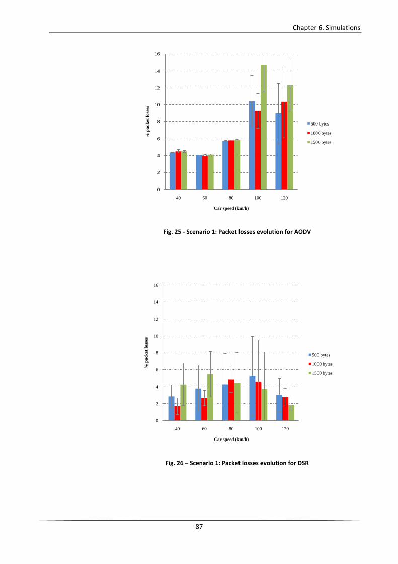
After the filtration, we reached the results as the following figures show.

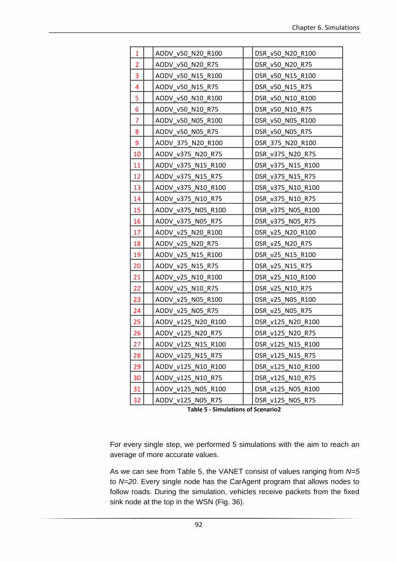
Fig.31, 32, 33 and 34 show us the AODV results in case of R=100m; They

show us, more or less, the average trend of the second scenario: high

percentage of packet losses and low throughput. In this particular case we

can see a few changes in terms of velocity. All the percentage remain

between 79% and 98% for the worst cases. The highest packet losses we

found are for N=15 and N=20 (Fig.31 and 32); the reason is simply

because increasing the number of cars on the road, the number of

collisions increase too, and this causes an higher percentage of packet

losses.

Looking at Fig.32, it seems to have a drastic decrease of losses for N=05

and N=10. But looking at Fig.31 we can see that in terms of percentage

level, the packet losses are only a little bit less than the other. The reason

is just because with N=05 and N=10, we have less cars in the road, and

therefore less routing-nodes. For this reason we can see from Fig.32 that

the total packet losses for N=05 and N=10 are about 5000, but just

because also the transmitted packets are much less than the other case

(N=15,20).

Fig. 31 - Scenario 2: Percentage of packet losses evolution for AODV and R=100

40

50

60

70

80

90

100

12,5 25 37,5 50

% p

ack

et l

oss

es

Car speed (km/h)

Packet losses

AODV_R100_20N

AODV_R100_15N

AODV_R100_10N

AODV_R100_05N


97

Fig. 32 - Scenario 2: Packet losses evolution for AODV and R=100

Fig. 33 - Scenario 2: AODV throughput with R=100

0

5000

10000

15000

20000

25000

30000

35000

12,5 25 37,5 50

Pac

kets

Car speed (km/h)

Total Packet losses

AODV_R100_20N

AODV_R100_15N

AODV_R100_10N

AODV_R100_05N

0

1

2

3

4

5

6

7

8

9

12,5 25 37,5 50

Th

rou

gh

pu

t (

KB

/s)

Car speed (km/h)

AODV_R100_20N

AODV_R100_15N

AODV_R100_10N

AODV_R100_05N


98

Fig. 34 – Scenario 2: End-to-end packet delay for AODV and R=100

In the case of R=75m, the transmission range decrease and the cars can

communicate and route only with the closest nodes. This causes a drastic

decrease in terms of number of communications. From Fig.35 and 36 we

can see that the best compromise between number of nodes (N), that helps

to forward the packets to a close routing-node, and number of

communications is for N=15 and N=20. In fact, a large number of cars allow

the node to forward easily and faster the received packet from an other

node.

Regarding the throughput results we can see from Fig.33 that for any

number of nodes, the number of bytes por second transmitted is not

changing considerably. The average value is about 6 Kbps, but we reach

higher values only for N=20.

Fig.34 and Fig.37 analyze the delay performances for the AODV protocol.

We can see clearly that with R=100 we have significant advantages with a

number of nodes equal to 15 or 20. With a less number of cars, values of

delay are acceptable with R=75.

0

10

20

30

40

50

60

12,5 25 37,5 50

del

ay

(s)

Car Speed (km/h)

AODV_R100_20N

AODV_R100_15N

AODV_R100_10N

AODV_R100_05N


99

Fig. 35 - Scenario 2: Percentage of packet losses evolution for AODV and R=75

Fig. 36 - Scenario 2: Packet losses evolution for AODV and R=75

40

50

60

70

80

90

100

12,5 25 37,5 50

% p

ack

et l

oss

es

Car speed (km/h)

Packet losses

AODV_R75_20N

AODV_R75_15N

AODV_R75_10N

AODV_R75_05N

0

5000

10000

15000

20000

25000

30000

35000

12,5 25 37,5 50

Pac

kets

Car speed (km/h)

Total Packet losses

AODV_R75_20N

AODV_R75_15N

AODV_R75_10N

AODV_R75_05N


100

Fig. 37 - Scenario 2: End-to-end packet delay for AODV and R=75

With the DSR protocol, NCTUns had some problems with N>10 and for this

reason the results are limited to the cases with N=05 and N=10. Regarding

the packet losses for R=100, the graphs in Fig.38 and Fig.39 show us values

close to the AODV protocol. But in Fig.40 it is important to note the

decreasing trend with always faster speed: the throughput arrives to 4 Kbps

for v=50Km/h, while it arrives to 6 Kbps for slower speeds (v=12,5 and v=25

Km/h).

0

10

20

30

40

50

60

12,5 25 37,5 50

del

ay

(s)

Car Speed (km/h)

AODV_R75_20N

AODV_R75_15N

AODV_R75_10N

AODV_R75_05N


101

Fig. 38 - Scenario 2: Percentage of packet losses evolution for DSR and R=100

Fig. 39 - Scenario 2: Packet losses evolution for DSR and R=100

40

50

60

70

80

90

100

12,5 25 37,5 50

% p

ack

et l

oss

es

Car speed (km/h)

Packet losses

DSR_R100_10N

DSR_R100_05N

0

5000

10000

15000

20000

25000

30000

35000

12,5 25 37,5 50

Pac

kets

Car speed (km/h)

Total Packet losses

DSR_R100_10N

DSR_R100_05N


102

Fig. 40 - Scenario 2: DSR throughput with R=100

Fig. 41 - Scenario 2: End-to-end packet delay for DSR and R=100

But with a less transmission range (R=75), the performances of DSR hint to

increase: a throughput average of 2Kbps create big disadvantages in the

network economy (Fig.44), but the delay-results give us an encouraging

scenario (Fig.41 and Fig.45).

0

1

2

3

4

5

6

7

8

9

12,5 25 37,5 50

Th

rou

gh

pu

t(K

B/s

)

Car speed (Km/h)

DSR_R100_10N

DSR_R100_05N

0

5

10

15

20

25

12,5 25 37,5 50

del

ay

(s)

Car Speed (km/h)

DSR_R100_10N

DSR_R100_05N


103

Fig. 42 - Scenario 2: Percentage of packet losses evolution for DSR and R=75

Fig. 43 - Scenario 2: Packet losses evolution for DSR and R=75

40

50

60

70

80

90

100

12,5 25 37,5 50

% p

ack

et

loss

es

Car speed (km/h)

Packet losses

DSR_R75_10N

DSR_R75_05N

0

5000

10000

15000

20000

25000

30000

35000

12,5 25 37,5 50

Pac

kets

Car speed (km/h)

Total Packet losses

DSR_R75_10N

DSR_R75_05N


104

Fig. 44 - Scenario 2: DSR throughput with R=75

Fig. 45 - Scenario 2: End-to-end packet delay for DSR and R=75

0

1

2

3

4

5

6

7

8

9

12,5 25 37,5 50

Th

rou

gh

pu

t(K

B/s

)

Car speed (Km/h)

DSR_R75_10N

DSR_R75_05N

0

5

10

15

20

25

12,5 25 37,5 50

del

ay

(s)

Car Speed (km/h)

DSR_R75_10N

DSR_R75_05N


105

According to the results for this second scenario it can be seen that DSR

performs better than AODV in terms of delay for every car speed. But if we

concentrate on the throughput, the average values calculated for AODV

gave us a faster data transmission than DSR.

Analyzing the various node‟s velocities, DSR show us best results for slow

speeds (v=12,5 and v=25 Km/h) for what concerning the throughput, but

looking at the delay graphs, increasing the node-speed, the delay decrease

always more. On the other hand is curious to see that the AODV behaviour

doesn‟t seem to change for values between 12,5 and 50 Km/h.

6.4 Problems found during simulations

As we mentioned before, NCTUns is a freeware software, and for this reason

the performances are not always at the top.

One of the biggest problems we met up during the simulations appears after the

“step R”. In fact, immediatly after the beginning of the simulation process, may

occur, for unknown reasons, that the program crashes. Sometimes the reasons

may be clear (incorrect modification of the map, different car speeds, ...), but

most of the time, when this type of problem appears, there are no reasons: the

same configuration with the same parameters may go or not. This type of crash

has led to a considerable loss of time. In fact, after every crash, we had to start

a sort of “recovery-process”, resumed in these steps:

Analyze the NCTUns processes that are still working after the crash

through the command:

ps aux | grep nctuns

“kill” all the processes that are close to our crashed-simulation. For

example all the lines that includes “CarAgent”, transmission commands,

... through the command:

kill PROCESS_IDNUMBER


106

Unfortunately, the processes to “kill” after the crash depend on the number of cars present on the simulation-map: the proportion is 2:1. So, everytime there was a crash, for example in a N=20 scenario, the processes to kill were 20x2 = 40.

In addition, an essential characteristic of a virtual machine is that the software running inside is limited to the resources and abstractions provided by the virtual machine and it cannot break out of its virtual world. For this reason file-transfer from an operative system to the other one, was not an immediate action and it was necessary to use a pen-drive recognized by both the operative systems.

Chapter 7. Conclusions and future work

107


In this work we have shown the performance of the routing protocols AODV and DSR in a

HSVN framework that includes a proposal for a communications protocol between WSNs

and VANETs. Simulation results show the better performance of AODV for high speed

scenarios (motorway) and of DSR for low speed scenarios (urban). All the simulation

strategies have been tested and compared to the simple geographic forwarding protocol

for various settings (network size and MS mobility pattern).

The proposed solutions have been tested against a simple flooding algorithm in order to

evaluate their efficiency and the overhead due to the transmission of control packets.

Possible research directions include the design and testing of appropriate buffer

management strategies. Data aggregation and data fusion algorithms shall also be in

order to complete the study on the depicted application scenario.

Developing the project, the following steps could summarize some future research lines

that has been deduced:

Modify the routing protocol to include some additional features suitable for vehicular network (location, speed, etc).

Analyze the different type of traffics (e.g. warnings, road messages, video-streaming, Internet browsing), the different QoS requirements according to the type of traffic, the several protocol interfaces that can be included into the vehicles (i.e. WIFI, 3G, satellite).

Results: high-priority warning messages will be sent through the best available connection, while video-streaming services can use another technology.

Analize other types of scenarios and settings.


108

Analyse the system performances under other more specific routing protocols for VANETs, e.g. GSR (Geographic Source Routing) [56], SAR (Spatial Aware Routing) [57], and VADD (Vehicular Assisted Data Delivery) [58].

Use the MAC IEEE 802.11p specification, which is focused on VANETs

Chapter 8. References and bibliography

109

Chapter 8. References and Bibliography

[1]. CVIS. Cooperative Vehicular -Infrastructure Systems. http://www.cvisproject.org/.

[2]. COME. Co-operative Intelligent Road Transport Systems: Vehicle-to-Vehicle and Vehicle-to-

Infrastructure communications. http://www.comesafety.org/.

[3]. NCTUns 6.0 (Network Simulator and Emulator). http://nsl.csie.nctu.edu.tw/nctuns.html. 2010.

[4]. C. Siva Ram Murthy, B.S. Manoj. Ad Hoc Network. “Ad Hoc Wireless Networks: Architectures and

Protocols”. June 3, 2004. ISBN: 978-0131470231.

[5]. K. Sohraby, D. Minoli, T. Znati. WSNs. “Wireless Sensor Networks: Technology, protocols and

applications”. Wiley Interscience : s.n., 2007. ISBN: 978-0-471-74300-2.

[6]. H. Hartenstein, K. Laberteaux. VANETs. “VANET Vehicular Applications and Inter-Networking

Technologies (Intelligent Transportation Systems)”. Wiley : s.n., March 2010. ISBN: 978-0470740569.

[7]. S. Olariu, M. Weigle. Vehicular Networks. “Vehicular Networks from Theory to Practice”. Norfolk

Virginia, USA : Chapman and Hall, 2009. ISBN: 978-1420085884.

[8]. D. Jiang, L. Delgrossi. IEEE 802.11p. “IEEE 802.11p: Towards an International Standard for Wireless

Access in Vehicular Environment”. Singapore, 67th IEEE Vehicular Technology Conference VTC : s.n., 2008.

[9]. IEEE P802.11p/D3.0. “Draft Amendment to Standard for Information Technology-Telecommunications

and Information Exchange between Systems-Local and Metropolitan Area Networks-Specific Requirements".

2007. Vol. Part 11: Wireless LAN Medium Access Control (MAC) and Physical Layer (PHY) Specifications-

Amendment 7: Wireless Access in Vehicular Environment.

[10]. B. Hofman-Wellenhof, H. Lichtenegger, J. Collins. GPS. “Global Positioning System: Theory and

Practice”. Springer : s.n., 2001. Vol. 5th Ed. ISBN: 3211835342.

[11]. TomTom. http://www.tomtom.com/.

[12]. GARMIN. http://www.garmin.com/garmin/cms/site/es.


110

[13]. D. Djenouri, E. Nekka, W. Soualhi. 1st ICST Int. Conf. On Ambient Media and Systems (Ambi-sys).

“Simulation of Mobility Models in Vehicular Ad hoc Networks”. Quebec, Canada, 2008. ISBN: 978-

9639799165.

[14]. F. Bai, N. Sadagopan, A. Helmy. The 22th IEEE Annual Joint Conference on Computer Communications

and Networking INFOCOM'03. “Important: a framework to systematically analyse the impact of mobility on

performance of routing protocols for ad hoc networks”. 2003. 825-835.

[15]. Davies, V. CSM (City Section Mobility), Tech. Rep. Master's thesis. “Evaluating mobility models within

an ad hoc network". Colorado School of Mines, Colorado, USA,2000.

[16]. A. Mahajan, N. Potnis, K. Gopalan, A. I. A. Wang. Proceedings of the 2nd IEEE International Workshop

on Next Generation Wireless Networks. "Urban mobility models for vanets". December 2006.

[17]. D. R. Choffnes, F. E. Bustamante. 2nd ACM international workshop on Vehicular ad hoc networks,

VANET'05. “An integrated mobility and traffic model for vehicular wireless networks".

[18]. C2C. Car-To-Car Communication Consortium. http://car-to-car.org/.

[19]. CARLINK. Wireless Traffic Service Platform for Linking Cars. http://carlink.lcc.uma.es/.

[20]. eSafety Forum. http://www.esafetysupport.org/.

[21]. INFOTRANSIT. Reial Automòbil Club de Catalunya (RACC). http://infotransit.es.

[22]. Google Maps. http://maps.google.com/.

[23]. F. Kong, J. Tan. IEEE International Conference on Information and Automation. “A Collaboration-based

Hybrid Vehicular Sensor Network Architecture”. Zhangjiajie, China, 2008.

[24]. J. Bohli, O. Ugus, D. Westhoff. ACM Workshop on Wireless Security. “A Secure and Resilient WSN

Roadside Architecture for Intelligent Transport System”. Alexandria, Virginia, USA, 2008.

[25]. E. Hossain, G. Chow, V. Leung, R. McLeod, J. Mišic, V. Wong, O. Yang. “Vehicular telematics over

heterogeneous wireless networks: A survey. Computer Communications”. Elsevier, 2010. pp. 775–793.

[26]. Bret Hull, Vladimir Bychkovsky, Yang Zhang, Kevin Chen, Michel Goraczko, Allen Miu, Eugene Shih,

Hari Balakrishnan, and Samuel Madden. Cartel: a distributed mobile sensor computing system.

Proceedings of the 4th international conference on Embedded networked sensor system. New York, NY,

USA, 2006. pp 125-138.

[27]. Lee, Uichin, et al. Mobeyes: smart mobs for urban monitoring with vehicular sensor network.

"Wireless Communications, IEEE" . October 2006. 13(5): 52-57.

[28]. Kutscher, J.Ottand D. Drive-thru internet: Ieee 802.11b for automobile users. "23rd Annual IEEE

Conference on Computer Communications (INFOCOM). 2004.

[29]. Vladimir Bychkovsky, Bret Hull, Allen Miu, Hari Balakrishnan, and Samuel Madden. A meaurement

study of vehicular internet access using in situ wi-fi networks. "Proceedings of the 12th annual international

conference on Mobile computing and networking". New York, NY, USA, 2006. pp 50-61.


111

[30]. David Hadaller, Srinivasan Keshav, Tim Brecht, and Shubham Agarwal. Vehicular opportunistic

communication under the microscope. "Proceedings of the 5th international conference on Mobile systems,

applications and services. New York, NY, USA, 2007. pp 206-219.

[31]. AndrewT.Campbell, ShaneB.Eisenman,NicholasD.Lane,Emiliano Miluzzo, and Ronald A. Peterson.

People-centric urban sensing. Proceedings of the 2nd annual international workshop on Wireless internet".

New York, NY, USA, 2006. pp 18.

[32]. Yang Zhang, Bret Hull, Vladimir Bychkovsky, Hari Balakrishnan, and Samuel Madden. Icedb:

Continuous query processing in an intermittently connected world. 2007.

[33]. Uichin Lee, Eugenio Magistretti, Biao Zhou, Mario Gerla, Paolo Bellavista, and Antonio Corradi.

Efficient data harvesting in mobile sensor platforms. Proceedings of the 4th annual IEEE international

conference Pervasive Computing and Communications Workshops. Washington, DC, USA : IEEE Computer

Society, 2006.

[34]. Hao Wu, Richard Fujimoto, Randall Guensler, and Michael Hunter. Mddv: a mobility-centric data

dissemination algorithm for vehicular networks. Proceedings of the 1st ACM international workshop on

Vehicular ad hoc networks. New York, NY, USA, ACM, 2004. pp 47-56.

[35]. Cao, J. Zhao and G. Vadd: Vehicle-assisted data delivery in vehicular ad hoc networks. INFOCOM 2006.

25th IEEE International Conference on Computer Communications. April 2006. pp 1-12.

[36]. M. D. Dikaiakos, A. Florides, T. Nadeem, and L. Iftode. Location-aware services over vehicular ad-hoc

networks using car-to-car communication. Selected Areas in Communications, IEEE Journal on. October

2007. 25(8): 1590-1602.

[37]. Jungkeun Yoon, Brian Noble, and Mingyan Liu. Surface street traffic estimation. MobiSys 07:

Proceedings of the 5th international conference on Mobile system, applications and services. New York, NY,

USA, ACM, 2007. pp 220-232.

[38]. D. Tacconi, I. Carreras, D. Miorandi, I. Chlamtac, F. Chiti, R. Fantacci. Supporting the sink mobility: a

case study for wireless sensor networks, in: Proc. of IEEE ICC. Glasgow, Scotland, 2007.

[39]. D. Tacconi, I. Carreras, D. Miorandi, F. Chiti, A. Casile, R. Fantacci. A system architecture supporting

mobile applications in disconnected sensor networks, in: Proc. of GLOBECOM. Washington, USA, 2007.

[40]. David Tacconi, Daniele Miorandi, Iacopo Carreras, Francesco Chiti, Romano Fantacci. Using wireless

sensor networks to support intelligent transportation systems. Florence, Italy, January 2010.

[41]. Y. Nam, H. Lee, H. Jung, T. Kwon, Y. Choi. An adaptive MAC (A-MAC) protocol guaranteeing network

lifetime for wireless sensor networks, in: Proc. of EW. Athens, Greece, 2006.

[42]. J. Polastre, J. Hill, D. Culler. Versatile low power media access for wireless sensor networks, in: Proc.

of ACM SenSys. New York, NY, USA, 2004.

[43]. Kung, S.Y. Wang and H.T. “A Simple Methodology for Constructing Extensible and High-Fidelity TCP/IP

Network Simulators" IEEE INFOCOM '99. New York, USA : s.n., March 1999.


112

[44]. Harvard TCP/IP network simulator 1.0, available at

http://www.eecs.harvard.edu/networking/simulator.html.

[45]. Stevens, Gray R. Wright and Richard. “TCP/IP Illustrated Volume 2” . Addison Wesely, 1995.

[46]. S. McCanne, S. Floyd. ns-LBNL Network Simulator (http://www-nrg.ee.lb.gov/ns/).

[47]. Keshav, S. “REAL: A Network Simulator” Technical Report, Dept. of computer Science. UC Berkeley,

1988.

[48]. OPNET Technologies, Inc. home page, http://www.opnet.com/products/home.html.

[49]. Vahalia, Uresh. “UNIX Internals: the New Frontiers” . Prentice-Hall, 1996.

[50]. Stevens, W. Richard. “UNIX Network Programming Volume 1, Networking APIs: Socket and XTI".

Prentice-Hall, 1998.

[51]. S. Y. Wang, C. L. Chou, and C. C. Lin. "The design and implementation of the NCTUns" Science Direct.

September 2006.

[52]. Smith, James E. e Nair, Ravi. "The Architecture of Virtual Machines". Computer (IEEE Computer

Society). 2005. 38 (5): 32–38.

[53]. Fanyu Kong, Jindong Tan. A Collaboration-based Hybrid Vehicular Sensor Network Architecture.

Houghton, Michigan, June 2008.

[54]. R. Baumann, S. Heimlicher, and M. May. Towards realistic mobility models for vehicular ad-hoc

networks. "Mobile Networking for Vehicular Environments". 2007. pp 73-78.

[55]. Ad hoc On-Demand Distance Vector (AODV) Routing. http://www.ietf.org/rfc/rfc3561.txt.

[56]. The Dynamic Source Routing Protocol (DSR. http://www.rfc-editor.org/rfc/rfc4728.txt.

[57]. C. Lochert, H. Hartenstein, J. Tian, H. Füßler, D. Hermann, M. Mauve. "A Routing Strategy for

Vehicular Ad Hoc Networks in City", IEEE Intelligent Vehicles Symposium '03. 2003. pp. 156-161.

[58]. J. Tian, L. Han,K. Rothermel. "Spatially Aware Packet Routing for Mobile Ad Hoc Inter-Vehicle Radio

Networks". IEEE Intelligent Transportation Systems. Shanghai, China, 2003. pp. 1546-1551.

[59]. J. Zhao, J. Cao. "VADD: Vehicle-assisted data delivery in vehicular ad hoc networks". 25th IEEE

International Conference on Computer Communications. 2006. pp.1-12.

[60]. Carolina Tripp Barba, Karen Ornelas, Monica Aguilar Igartua. “Performance Evaluation of a Hybrid

Sensor and Vehicular Network to improve road safety”. Accepted, Pending to pubblication, PE-WASUN,

October 17-21, Bodrum, Turkey, 2010.

Date post:	03-Feb-2022
Category:	Documents
Upload:	others
View:	5 times
Download:	0 times

Performance Evaluation of Vehicular Ad Hoc Networks using

Documents