Performance Indicator – Horizontal Flight Efficiency · KEP Key performance Environment indicator...

Performance Indicator – Horizontal Flight Efficiency Level 1 and 2 documentation of the Horizontal Flight Efficiency key performance indicators

Overview This document is a template for a Level 1 & Level 2 document for the Horizontal Flight Efficiency Indicators – KEP and KEA.

The approved version of this document is quality controlled as part of the PRU (prototype) Quality Management System.

Edition Number: 01-00 Edition Date: 23/05/2014 Status: First Release Intended For: Internal and Stakeholders Category: Performance Monitoring and Reporting – Level 1/2

European Organization for Safety of Air Navigation

Performance Indicator – Horizontal Flight Efficiency – Edition 01-00 Page i

TITLE

Performance Indicator – Horizontal Flight Efficiency

Publications Reference: ISBN Number:

Document Identifier Edition Number: 01-00

EUROCONTROL KPI_descr_KEP_KEA Edition Date: 23/05/2014 Abstract

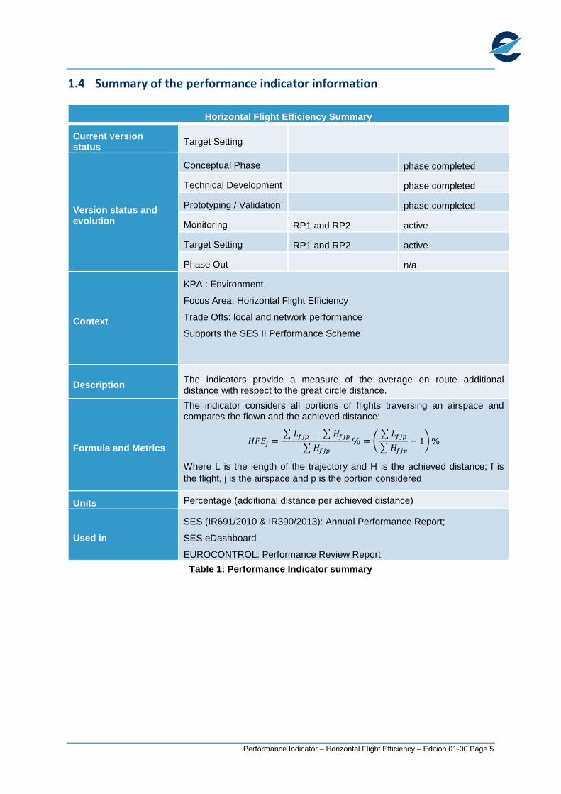
This document describes conceptual, informational and mathematical, and platform independent model of Horizontal Flight Efficiency Indicators – KEP and KEA

Keywords Key Performance Indicator Horizontal Flight Efficiency Data Processing

Authority Name Unit

Document Author Guglielmo Guastalla PRU

Document Reviewer Elsa Freville PRU

Document Approver Bernd Tiemayer PRU

Performance Indicator – Horizontal Flight Efficiency – Edition 01-00 Page i

Table of Contents

1. INTRODUCTION ................................................................................................................... 4

1.1 General .............................................................................................................................. 4

1.2 Purpose of the document ................................................................................................... 4

1.3 Scope ................................................................................................................................. 4

1.4 Summary of the performance indicator information .......................................................... 5

1.5 Acronyms and terminology ................................................................................................ 6

2. CONCEPTUAL MODEL THE HORIZONTAL FLIGHT EFFICIENCY ................................... 7

2.1 The achieved distance ....................................................................................................... 8

2.2 Achieved distances and network contribution ................................................................... 9

2.3 Decomposition of inefficiency in local and interface components ................................... 10

2.4 Independence of local performance from performance outside the local area ............... 10

2.5 Summary of the different quantities ................................................................................. 11

2.6 Aggregation of results to produce the indicator ............................................................... 11

2.7 Difference between KEP and KEA .................................................................................. 12

2.8 Specific/special cases and FAQ ...................................................................................... 12

3. DATA FLOWS AND PROCESSES ..................................................................................... 15

3.1 Data processing ............................................................................................................... 16

3.2 Data completeness .......................................................................................................... 16

3.3 Trajectory Eligibility .......................................................................................................... 16

3.4 Data consistency ............................................................................................................. 17

4. INFORMATION AVAILABLE ............................................................................................... 17

5. QUALITY MANAGEMENT................................................................................................... 22

6. REFERENCES .................................................................................................................... 23

7. REVISION HISTORY ........................................................................................................... 23

List of Figures Figure 1: HFE as comparison of flight length and Great Circle Distance .......................................................... 7 Figure 2: Local Performance Requirement........................................................................................................ 7 Figure 3: The two Quantities Averaged in the Achieved Distance .................................................................... 8 Figure 4: A case of perfect local efficiency with no network contribution .......................................................... 9 Figure 5: Decomposition of Inefficiency ........................................................................................................... 10 Figure 6: Independence of local performance from performance outside the local area ................................ 10 Figure 7: Data Flows ........................................................................................................................................ 15

Performance Indicator – Horizontal Flight Efficiency – Edition 01-00 Page ii

List of Tables Table 1: Performance Indicator summary ......................................................................................................... 5 Table 2: Acronyms and terminology .................................................................................................................. 6 Table 3: Summary of the different quantities used to compute HFE ............................................................... 11 Table 4: General location of origin, destination and en-route end-points ........................................................ 13 Table 5: Airspace profile data .......................................................................................................................... 18 Table 6: Circle profile data ............................................................................................................................... 18 Table 7: Point profile data ................................................................................................................................ 19 Table 8: Airspace definitions data ................................................................................................................... 19 Table 9: Flight data .......................................................................................................................................... 21 Table 10: Measured airspaces data ................................................................................................................ 21 Table 11: Flights Statistics ............................................................................................................................... 22 Table 12: Airspaces Statistics ......................................................................................................................... 22

Performance Indicator – Horizontal Flight Efficiency – Edition 01-00 Page iii

1. Introduction

1.1 General

This document describes the conceptual, informational, and implementation independent model of the Horizontal Flight Efficiency Indicators – KEP and KEA.

The indicator is used as part of the performance monitoring and reporting under:

SES: IR691/2010 and IR390/2013; and

EUROCONTROL: performance review reporting.

1.2 Purpose of the document

The purpose of this document is to provide a description of the horizontal flight efficiency indicator and its two versions used in the Performance Scheme Regulation – KEP and KEA. It addresses different audiences with different needs, and for that reason the description is provided at increasing level of detail.

Section 2 provides a high level description of the indicator, introduces the concept of achieved distance and provides the rationale for its use as the base for the computation of the additional distance (i.e., the balance of the need to evaluate local performance with the need to take into consideration its impact on the measurement of network performance). It includes a final subsection with some special cases and frequently asked questions which should help clarify how it is calculated.

Section 3 provides a description of the data available within the Performance Scheme Regulation and how it is treated to produce the official indicators. It sketches a description of the envisaged data quality approach, which relies on clearly separating the different stages in the data flow. Coupled with openness and transparency in the treatment of data it fosters cooperation between the different stakeholders.

Section 4 provides details about the main content of the tables used to perform and store the calculations.

1.3 Scope

This document covers the data processing and calculation of the Horizontal Flight Efficiency key performance indicators (KEP and KEA).

The calculation of this performance indicator is performed according to the Horizontal Flight Efficiency Data Flow standard for data collection and processing, under the responsibility of the operations unit in the QoS department of the PRU, which is compliant with IR691/2010 and IR390/2013. The Horizontal Flight Efficiency Data Flow associated processes and procedures are documented as part of the PRU Quality Management System.

These key performance indicators are also defined in the Implementing Regulation (390/2013), Annex I:

• Section 1, Environment 2.1, (a) (KEA, Union-wide level);

• Section 1, Environment 2.1 (b) (KEP, Union-wide level);

• Section 2, Environment 2.1 (KEA, Functional Airspace Block level);

Performance Indicator – Horizontal Flight Efficiency – Edition 01-00 Page 4

1.4 Summary of the performance indicator information

Horizontal Flight Efficiency Summary Current version status Target Setting

Version status and evolution

Conceptual Phase

phase completed Technical Development

phase completed

Prototyping / Validation

phase completed Monitoring RP1 and RP2 active Target Setting RP1 and RP2 active Phase Out n/a

Context

KPA : Environment Focus Area: Horizontal Flight Efficiency Trade Offs: local and network performance Supports the SES II Performance Scheme

Description The indicators provide a measure of the average en route additional distance with respect to the great circle distance.

Formula and Metrics

The indicator considers all portions of flights traversing an airspace and compares the flown and the achieved distance:

𝐻𝐹𝐸𝑗 =�𝐿𝑓𝑗𝑝 −�𝐻𝑓𝑗𝑝

�𝐻𝑓𝑗𝑝% = �

�𝐿𝑓𝑗𝑝�𝐻𝑓𝑗𝑝

− 1�%

Where L is the length of the trajectory and H is the achieved distance; f is the flight, j is the airspace and p is the portion considered

Units Percentage (additional distance per achieved distance)

Used in SES (IR691/2010 & IR390/2013): Annual Performance Report;

SES eDashboard

EUROCONTROL: Performance Review Report Table 1: Performance Indicator summary


1.5 Acronyms and terminology

Term Definition

ANSP Air Navigation Service Provider

ATFM Air Traffic Flow Management

ATM Air Traffic Management

CPF Profile based on correlated positions report

CPR Correlated Position Report

DB Database

EU European Union

FAB Functional Airspace Block

FAQ Frequently Asked Questions

FIR Flight Information Region

FTFM Last filed flight plan

GCD Great Circle Distance

HFE Horizontal Flight Efficiency

ICAO International Civil Aviation Organization

ID Identifier

IR691 COMMISSION REGULATION (EU) No 691/2010

IR390 COMMISSION REGULATION (EU) No 390/2013

KEA Key performance Environment indicator based on Actual trajectory

KEP Key performance Environment indicator based on last filed flight Plan

KPA Key Performance Area

KPI Key Performance Indicator

LOBT Last Off-Block Time

NM Network Manager

PRR Performance Review Report

PRU Performance Review Unit

QoS Quality of Service

RP1 1st Reference Period (2012-2014)

RP2 2nd Reference Period (2015-2019)

SES Single European Sky

TMA Terminal Manoeuvring Area Table 2: Acronyms and terminology


2. Conceptual model The Horizontal Flight Efficiency

Horizontal flight efficiency (HFE) is very simply defined at its highest level: the comparison between the length of a trajectory and the shortest distance between its endpoints.

Figure 1: HFE as comparison of flight length and Great Circle Distance

For an entire flight we want to calculate the additional distance flown between take-off and landing with respect to the most direct route between the two airports (Great Circle Distance). The need of a more detailed definition arises because we need to take into consideration different variations from the situation described above, such as the possibility that one (if not both) of the airports does not belong to the area on which we would like to measure the efficiency and the need to define the measurement on a portion of the flight (e.g., en route) instead than for the whole trajectory.

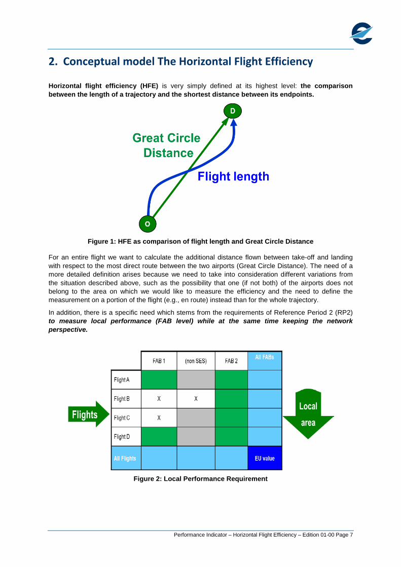
In addition, there is a specific need which stems from the requirements of Reference Period 2 (RP2) to measure local performance (FAB level) while at the same time keeping the network perspective.

Figure 2: Local Performance Requirement


The desired outcome is illustrated in the table above. We are interested in all flights which traverse at least in part the Single European Sky (SES) area. A flight might traverse several FABs but also areas which are not part of the SES area. This means that, for the purpose of measuring flight efficiency in the SES area, we are interested only in the values in the green cells of the table. At the same time we would like to be able to consider the additional distances along the flight dimension (i.e., along a row, giving a flight value in the light blue cell in the last column) and along the FAB dimension (i.e., along a column, giving a FAB value in the light blue cell in the last row) and obtain consistent values. The sum of the all values in the green cells, the sum of all values in the last column (i.e. sum of flight values) and the sum of all values in the last row (i.e., sum of the FAB values) should all be the same (i.e., using flight values and using FAB values should lead to the same sum when considering all flights in the SES area).

This is true when the values in the table correspond to the flown distance and the achieved distance (defined in the following section), which allows to apportion the great circle distance for the entire trajectory to any of its parts, e.g., between the entry and exit into a FAB.

2.1 The achieved distance

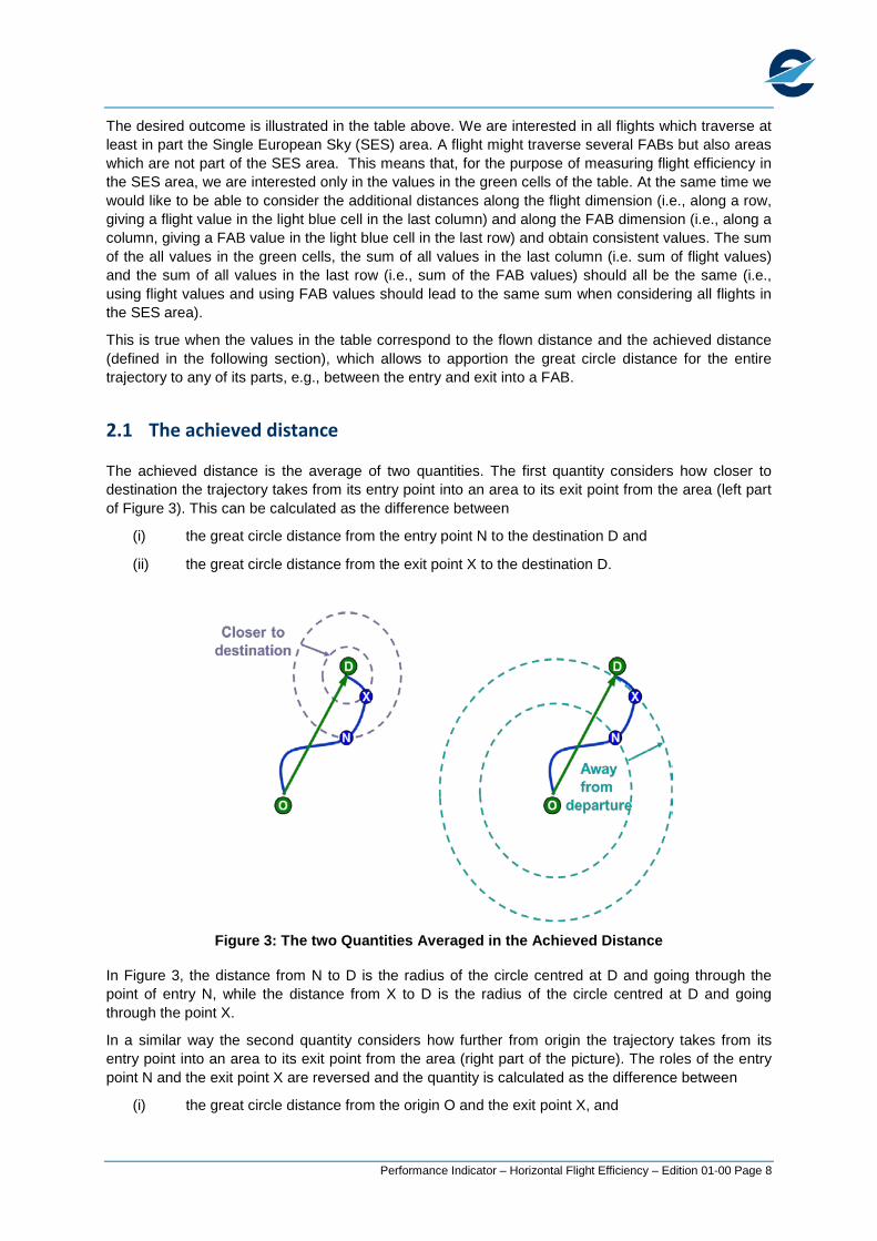
The achieved distance is the average of two quantities. The first quantity considers how closer to destination the trajectory takes from its entry point into an area to its exit point from the area (left part of Figure 3). This can be calculated as the difference between

(i) the great circle distance from the entry point N to the destination D and

(ii) the great circle distance from the exit point X to the destination D.

Figure 3: The two Quantities Averaged in the Achieved Distance

In Figure 3, the distance from N to D is the radius of the circle centred at D and going through the point of entry N, while the distance from X to D is the radius of the circle centred at D and going through the point X.

In a similar way the second quantity considers how further from origin the trajectory takes from its entry point into an area to its exit point from the area (right part of the picture). The roles of the entry point N and the exit point X are reversed and the quantity is calculated as the difference between

(i) the great circle distance from the origin O and the exit point X, and


(ii) the great circle distance from the origin O and the entry point N.

Considering two specific points along the trajectory (for example its entry point N and its exit point X into/from an area), together with the origin O and the destination D, the formula to compute the achieved distance is:

12

(𝑁𝐷 − 𝑋𝐷 + 𝑂𝑋 − 𝑂𝑁)

where all the distances between points are calculated as great circle distances.

It can be verified that taking a sequence of points between O and D, e.g., a sequence of entry/exit points in different areas, the sum of the achieved distances (including the one from the origin to the first point and the one from the last point to the destination) is equal to the great circle distance between the origin and the destination.

2.2 Achieved distances and network contribution

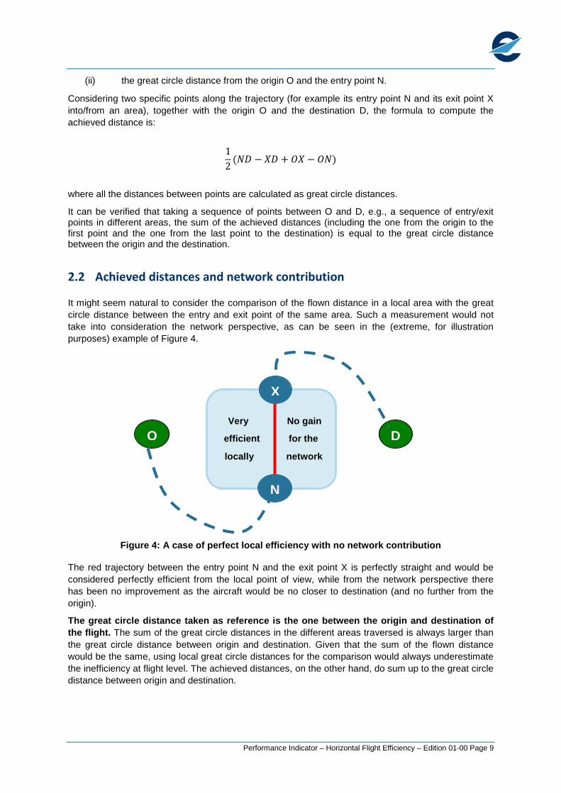
It might seem natural to consider the comparison of the flown distance in a local area with the great circle distance between the entry and exit point of the same area. Such a measurement would not take into consideration the network perspective, as can be seen in the (extreme, for illustration purposes) example of Figure 4.

Figure 4: A case of perfect local efficiency with no network contribution

The red trajectory between the entry point N and the exit point X is perfectly straight and would be considered perfectly efficient from the local point of view, while from the network perspective there has been no improvement as the aircraft would be no closer to destination (and no further from the origin).

The great circle distance taken as reference is the one between the origin and destination of the flight. The sum of the great circle distances in the different areas traversed is always larger than the great circle distance between origin and destination. Given that the sum of the flown distance would be the same, using local great circle distances for the comparison would always underestimate the inefficiency at flight level. The achieved distances, on the other hand, do sum up to the great circle distance between origin and destination.

Very No gain

efficient for the

locally network

O D

N

X


2.3 Decomposition of inefficiency in local and interface components

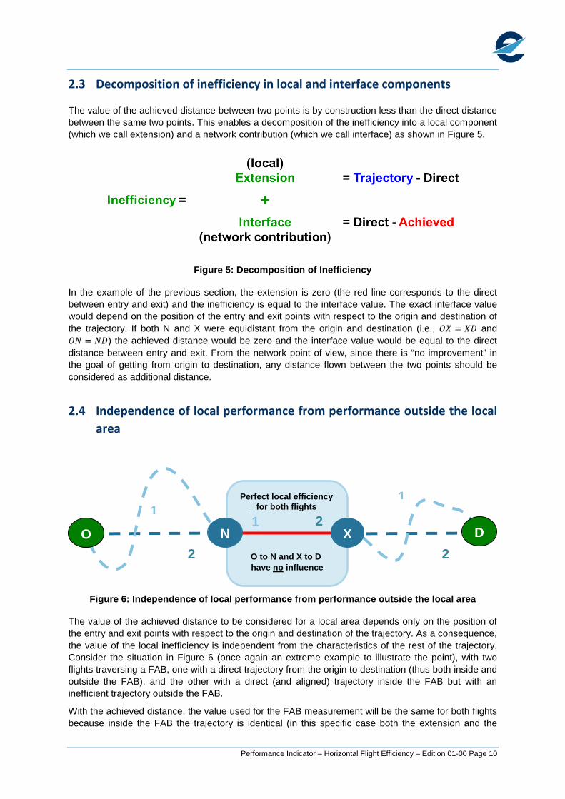
The value of the achieved distance between two points is by construction less than the direct distance between the same two points. This enables a decomposition of the inefficiency into a local component (which we call extension) and a network contribution (which we call interface) as shown in Figure 5.

Figure 5: Decomposition of Inefficiency

In the example of the previous section, the extension is zero (the red line corresponds to the direct between entry and exit) and the inefficiency is equal to the interface value. The exact interface value would depend on the position of the entry and exit points with respect to the origin and destination of the trajectory. If both N and X were equidistant from the origin and destination (i.e., 𝑂𝑋 = 𝑋𝐷 and 𝑂𝑁 = 𝑁𝐷) the achieved distance would be zero and the interface value would be equal to the direct distance between entry and exit. From the network point of view, since there is “no improvement” in the goal of getting from origin to destination, any distance flown between the two points should be considered as additional distance.

2.4 Independence of local performance from performance outside the local area

Figure 6: Independence of local performance from performance outside the local area

The value of the achieved distance to be considered for a local area depends only on the position of the entry and exit points with respect to the origin and destination of the trajectory. As a consequence, the value of the local inefficiency is independent from the characteristics of the rest of the trajectory. Consider the situation in Figure 6 (once again an extreme example to illustrate the point), with two flights traversing a FAB, one with a direct trajectory from the origin to destination (thus both inside and outside the FAB), and the other with a direct (and aligned) trajectory inside the FAB but with an inefficient trajectory outside the FAB.

With the achieved distance, the value used for the FAB measurement will be the same for both flights because inside the FAB the trajectory is identical (in this specific case both the extension and the

1 1

2 O D N X

Perfect local efficiency for both flights

O to N and X to D have no influence

2

1 2


interface will be zero, as the trajectory is direct between entry and exit and the entry and exit points are aligned with the origin and destination).

It has been proposed to compute the value of the local efficiency as the average, taken over all flights traversing the local area, of the entire trajectories. In the example above, while the two trajectories are identical within the FAB, their contribution would be different because the inefficiency of trajectory 1 outside the FAB will be taken into account (as a matter of fact, the calculation would not isolate the local performance). As a result, the inefficiency of the FAB will also be greater than zero.

2.5 Summary of the different quantities

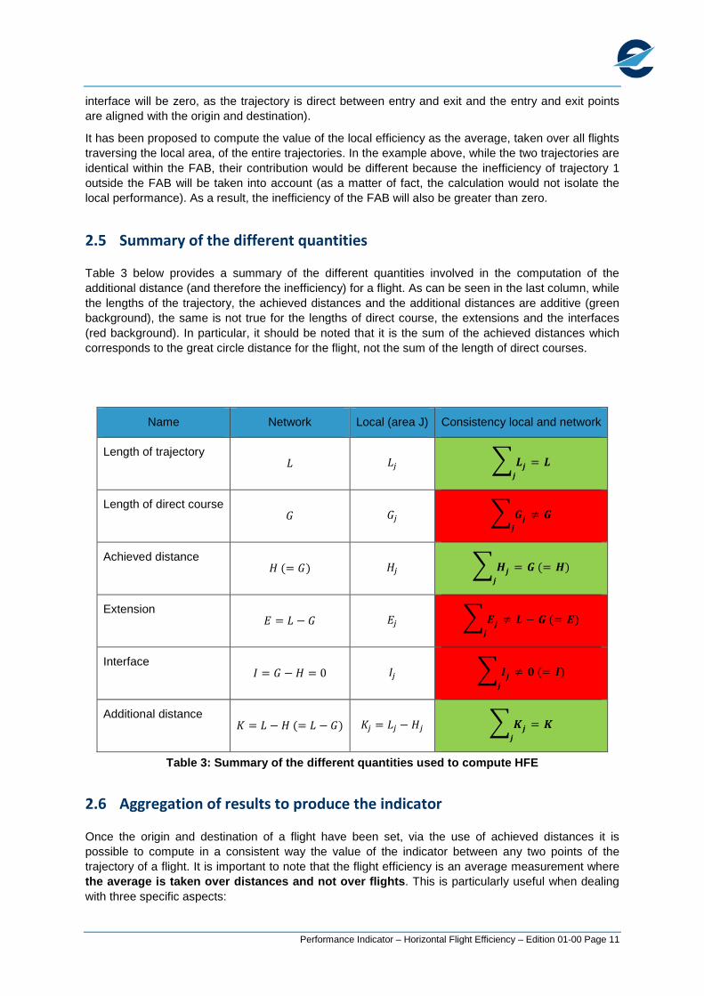
Table 3 below provides a summary of the different quantities involved in the computation of the additional distance (and therefore the inefficiency) for a flight. As can be seen in the last column, while the lengths of the trajectory, the achieved distances and the additional distances are additive (green background), the same is not true for the lengths of direct course, the extensions and the interfaces (red background). In particular, it should be noted that it is the sum of the achieved distances which corresponds to the great circle distance for the flight, not the sum of the length of direct courses.

Name Network Local (area J) Consistency local and network

Length of trajectory 𝐿 𝐿𝑗 �𝑳𝒋

𝒋= 𝑳

Length of direct course 𝐺 𝐺𝑗 �𝑮𝒋

𝒋≠ 𝑮

Achieved distance 𝐻 (= 𝐺) 𝐻𝑗 �𝑯𝒋

𝒋= 𝑮 (= 𝑯)

Extension 𝐸 = 𝐿 − 𝐺 𝐸𝑗 �𝑬𝒋

𝒋≠ 𝑳 − 𝑮 (= 𝑬)

Interface 𝐼 = 𝐺 − 𝐻 = 0 𝐼𝑗 �𝑰𝒋

𝒋≠ 𝟎 (= 𝑰)

Additional distance 𝐾 = 𝐿 − 𝐻 (= 𝐿 − 𝐺) 𝐾𝑗 = 𝐿𝑗 − 𝐻𝑗 �𝑲𝒋

𝒋= 𝑲

Table 3: Summary of the different quantities used to compute HFE

2.6 Aggregation of results to produce the indicator

Once the origin and destination of a flight have been set, via the use of achieved distances it is possible to compute in a consistent way the value of the indicator between any two points of the trajectory of a flight. It is important to note that the flight efficiency is an average measurement where the average is taken over distances and not over flights. This is particularly useful when dealing with three specific aspects:


• The measurement of the en-route flight inefficiency. The indicator is concerned with the en-route flight inefficiency defined as the measurement which excludes 40 nautical miles around airports. The measurement does not start until the trajectory has crossed (for the first time) the cylinder with a 40 nautical miles radius around the airport of departure and ends when the trajectory crosses (for the last time) the cylinder with a 40 nautical miles radius around the airport of arrival.

• The measurement of local inefficiencies. The indicator based on achieved distances is well defined even when the direct route between origin and destination does not cross the local area. It is also well defined when a trajectory exits and re-enters a local area (the two measurements are independent).

• The measurement of inefficiency when the trajectory is not complete (which might be the case for CPF trajectories). The measurement is well defined for every portion of the trajectory, and does not require a complete trajectory.

When looking at a specific flight, it is always possible to decompose the flight in different portions, of which some will not be taken into consideration for the calculation of the indicator (as an example, the first part of the trajectory will never be included because it will either be inside the 40 nautical miles or outside of the reference area). Every portion can be attributed to a specific measured area (e.g., a State, a FAB, the SES area).

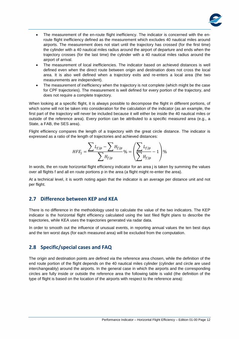
Flight efficiency compares the length of a trajectory with the great circle distance. The indicator is expressed as a ratio of the length of trajectories and achieved distances:

𝐻𝐹𝐸𝑗 =�𝐿𝑓𝑗𝑝 −�𝐻𝑓𝑗𝑝

�𝐻𝑓𝑗𝑝% = �

�𝐿𝑓𝑗𝑝

�𝐻𝑓𝑗𝑝− 1�%

In words, the en route horizontal flight efficiency indicator for an area j is taken by summing the values over all flights f and all en route portions p in the area (a flight might re-enter the area).

At a technical level, it is worth noting again that the indicator is an average per distance unit and not per flight.

2.7 Difference between KEP and KEA

There is no difference in the methodology used to calculate the value of the two indicators. The KEP indicator is the horizontal flight efficiency calculated using the last filed flight plans to describe the trajectories, while KEA uses the trajectories generated via radar data.

In order to smooth out the influence of unusual events, in reporting annual values the ten best days and the ten worst days (for each measured area) will be excluded from the computation.

2.8 Specific/special cases and FAQ

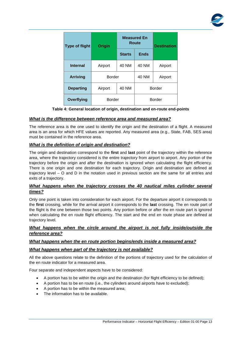
The origin and destination points are defined via the reference area chosen, while the definition of the end route portion of the flight depends on the 40 nautical miles cylinder (cylinder and circle are used interchangeably) around the airports. In the general case in which the airports and the corresponding circles are fully inside or outside the reference area the following table is valid (the definition of the type of flight is based on the location of the airports with respect to the reference area):


Type of flight Origin

Measured En Route

Destination

Starts Ends

Internal Airport 40 NM 40 NM Airport

Arriving Border 40 NM Airport

Departing Airport 40 NM Border

Overflying Border Border

Table 4: General location of origin, destination and en-route end-points

What is the difference between reference area and measured area? The reference area is the one used to identify the origin and the destination of a flight. A measured area is an area for which HFE values are reported. Any measured area (e.g., State, FAB, SES area) must be contained in the reference area.

What is the definition of origin and destination? The origin and destination correspond to the first and last point of the trajectory within the reference area, where the trajectory considered is the entire trajectory from airport to airport. Any portion of the trajectory before the origin and after the destination is ignored when calculating the flight efficiency. There is one origin and one destination for each trajectory. Origin and destination are defined at trajectory level – O and D in the notation used in previous section are the same for all entries and exits of a trajectory.

What happens when the trajectory crosses the 40 nautical miles cylinder several times? Only one point is taken into consideration for each airport. For the departure airport it corresponds to the first crossing, while for the arrival airport it corresponds to the last crossing. The en route part of the flight is the one between those two points. Any portion before or after the en route part is ignored when calculating the en route flight efficiency. The start and the end en route phase are defined at trajectory level.

What happens when the circle around the airport is not fully inside/outside the reference area?

What happens when the en route portion begins/ends inside a measured area?

What happens when part of the trajectory is not available? All the above questions relate to the definition of the portions of trajectory used for the calculation of the en route indicator for a measured area.

Four separate and independent aspects have to be considered:

• A portion has to be within the origin and the destination (for flight efficiency to be defined); • A portion has to be en route (i.e., the cylinders around airports have to excluded); • A portion has to be within the measured area; • The information has to be available.


The four conditions have to be valid at the same time. This means that in some cases the end points of the portion considered for flight efficiency in a measured area (the entry N and the exit X in the notation used in previous sections) will not correspond to the borders of the measured area.

The main reason for the entry/exit points not being on the border of the measured area is the exclusion of the circles around the airport (see table above and the following examples). A secondary reason is the absence of information for a part of a trajectory (see example below).

Consider the case of a flight departing from a measured area A, with the circle/cylinder entirely contained in the measurement area A. The origin (Of) will be the airport because it will be the first point into the reference area (a measured area is always part of the reference area). As the part within the cylinder has to be excluded when measuring the en route flight efficiency, the entry into the measured area (NA) will correspond to the first crossing of the (departure airport) cylinder. It is neither the airport (airports can never be the entry or exit point for en route flight efficiency because of the exclusion of the circle around them) nor the border of the measured area A. The situation corresponds to the standard “departing” or “internal” row in the table above.

Consider the same case above, except that the circle extends into another measured area B and the first crossing is happening there. The origin will still be located at the airport in measured area A, but there will be no portion of trajectory considered for measured area A because the en route part will not have started. The entry into measured area B (NB) will again correspond to the first crossing of the (departure airport) cylinder and not the airport or the border of measured area B.

As a third alternative, consider the case where the circle around area A extends outside the reference area, the first crossing happens there and the flight then re-enter measured area A. The origin will again be located at the airport; the en route portion will start outside the reference area; the first entry into area A (NA) will be the one from outside the reference area.

Last, consider the case where a flight traverses a measured area, with entry and exit on the borders but with a part of the trajectory for which the information is missing. In that case there will be two portions of the trajectory considered: the first one from the border (N1) until the information is lost (X1) and a second one from when the information is again available (N2) until the exit from the measured area (X2).

What happens when the trajectory enters an area several times? Every couple of entry and exit points (see the previous answer for why the entry and exit points might not correspond to points on the border of the measured area considered) defines a portion of the flight for which the length of the trajectory and the achieved distance can be calculated. All portions within a measured area are considered in the calculation of the indicator for that area.

It is important to note that multiple entries are considered separately and it is not the first point of entry and the last point of exit of a measured area which are considered (see last example in the previous question).

Can the achieved distance be negative? The achieved distance relies on the order of the points considered; it is therefore possible (although uncommon) for the local achieved distance to be negative. This ensures that the calculation of the local additional distances is consistent (any partition of the trajectory gives the same result).

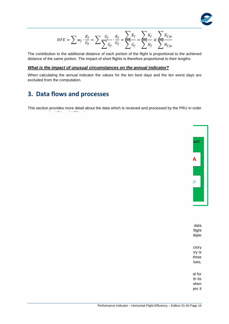
What is the impact of short flights (for which the great circle distance is small)? The horizontal flight efficiency (HFE) is not an average per flight, but a weighted average which takes into consideration the great circle distance (K is the additional distance, G is the great circle distance, H is the achieved distance; f indicates a flight, j indicates an area, p indicates a portion of the flight):


𝐻𝐹𝐸 = �𝑤𝑓 ∙𝐾𝑓𝐺𝑓

= �𝐺𝑓

�𝐺𝑓∙𝐾𝑓𝐺𝑓

=�𝐾𝑓

�𝐺𝑓=�𝐾𝑓

�𝐻𝑓≅�𝐾𝑓𝑗𝑝

�𝐻𝑓𝑗𝑝

The contribution to the additional distance of each portion of the flight is proportional to the achieved distance of the same portion. The impact of short flights is therefore proportional to their lengths.

What is the impact of unusual circumstances on the annual indicator? When calculating the annual indicator the values for the ten best days and the ten worst days are excluded from the computation.

3. Data flows and processes

This section provides more detail about the data which is received and processed by the PRU in order to generate the KEA and KEP values.

Figure 7: Data Flows

Figure 7 provides a very high level view of the data flow. The source and characteristics of the data received by the NM are of a different nature for what concerns flight plans and CPRs; while for flight plans there is a single source (last filed plan) defining the whole trajectory, for CPRs there are multiple sources of information which need to be “merged” in order to obtain a single trajectory.

In both cases the Network Manager processes the data received and produces a single trajectory (one called CPF from CPRs, one called FTFM derived from the last filed flight plan). The trajectory is described via three different “profiles” (point, airspace and cylinder – to be detailed later). The three profiles are stored into the PRISME DB, which is accessed by the PRU to produce the HFE values, together with the KEP and KEA indicators.

A clear definition of the different scopes (represented by the boxes in the figure above) is essential for data quality processes, as it enables to consider data processing in separate “modules”, each with its inputs, processes, and outputs. It is thus possible to consider each of them in separation when analysing and improving the data flow. Without a clear definition of the different processing stages it

Dashboard NM

P R I S ME

DB

CPRs

ANSPs

…

AUs

Plans

PRU

HFE Calculations

KEA

KEP HFE Calculations

CPFs (Points,

Airspaces, Cylinders)

FTFMs (Points,

Airspaces, Cylinders)


gguastal

Rectangle

Date post:	28-May-2019
Category:	Documents
Upload:	vukhanh
View:	232 times
Download:	0 times

Performance Indicator – Horizontal Flight Efficiency · KEP Key performance Environment indicator...

Documents