Performance Limits in Control with Application Educational...Performance Limits in Control with...

UNCLASSIFIED/UNLIMITED

Performance Limits in Control with Application to Communication Constrained UAV Systems

Prof. Dr. Richard H. Middleton ARC Centre for Complex Dynamic Systems and Control

The University of Newcastle, Callaghan NSW, Australia, 2308

[email protected]

ABSTRACT

The study of performance limitations in feedback control systems has a long history, commencing with Bode’s gain-phase and sensitivity integral formulae. This area of research focuses on questions of what aspects of closed loop performance can we reasonably demand, and what are the trade-offs or costs of achieving this performance. In particular, it considers concepts related to the inherent costs of stabilisation, limitations due to ‘non-minimum phase’ behaviour, time delays, bandwidth limitations etc. There are a range of results developed in the 90’s for multivariable linear systems, together with extensions to sampled data, non-linear systems. More recently, this work has been extended to consider communication limitations, such as bit-rate or signal to noise ratio limitations and quantization effects. This paper presents: (i) A review of work on performance limitations, including recent results; (ii) Results on impacts of communication constraints on feedback control performance; and (iii) Implications of these results on control of distributed UAVs in formation.

1.0 INTRODUCTION

In many control applications it is crucial that the factors limiting the performance of the system are identified. For example, closed loop control performance may be limited due to the fact that the actuators are too slow, or too inaccurate (perhaps due to complex nonlinear effects, such as backlash and hysteresis), to support the desired objectives. Alternatively, it may be that the measurement transducers lack the precision required. In some cases, model fidelity is important to the performance, and the process complexities may make the task of modelling the process very difficult. A further class of limitations are those due to the inherent dynamics of the plant and the structure of the system. Factors in the plant dynamics that may inhibit the achievable performance include unstable plant poles, non-minimum phase behaviour and time delays. These limitations based on a plant features have been studied extensively over many years. More recently these results have been extended to include aspects of the overall system topology, including features such as network and communication based constraints on information transfer.

The study of performance limitations in feedback control systems is concerned with what may and may not be achieved in feedback control design, given plant characteristics. This area of research has a long history, with early results due to Bode [1] on the well known gain-phase relationship, and also the Bode sensitivity integral for linear, single input-single output, open loop stable continuous time systems. Some time later, Horowitz [2], in the context of control system synthesis, made use of the Bode sensitivity integral as a crucial element in the synthesis process in understanding when changes of one aspect of control performance would inevitably have deleterious affects on other aspects of performance. Early

RTO-EN-SCI-175 1 - 1


Middleton, R.H. (2007) Performance Limits in Control with Application to Communication Constrained UAV Systems. In System Control Technologies, Design Considerations & Integrated Optimization Factors for Distributed Nano UAV Applications (pp. 1-1 – 1-44). Educational Notes RTO-EN-SCI-175, Paper 1. Neuilly-sur-Seine, France: RTO. Available from: http://www.rto.nato.int.

http://www.rto.nato.int

mailto:[email protected]


UNCLASSIFIED/UNLIMITED UNCLASSIFIED/UNLIMITED

works in the field of H∞ optimal control using frequency domain ideas, frequently encountered performance limitation ideas, as right half plane plant poles and zeros appeared explicitly in the interpolation, and approximation problems (see for example [3]). It was perfectly natural therefore to consider the limitations imposed by poles and zeros in this context. Unfortunately, these limitations are not always transparent when the equations are represented in state space form (for example [4]), or the more recent linear matrix inequality forms [5], though these forms are very valuable for computational purposes.

More recently, there has been a great deal of interest in the extra challenges posed when implementing feedback control loops over a communication channel. The potential array of additional problems communication channels impose include variable transmission delays [6], occasional errors (including the possibility of missing or even repeated data) [7], quantisation [8], [9], [10], [11], bandwidth [12], and data rate limits [13], [14], [15], [16], [17]. Here we follow largely the later line of research, namely, data rate limitations, though we view this from the point of view of information theory and finite capacity feedback, and signal to noise ratio constrained feedback systems [18].

In a third line of work, there has been extensive interest in consensus or distributed control problems in recent years. One aspect of this is distributed formation control problems, the one dimensional version of which have been studied in the context of intelligent vehicle highway systems, or vehicle platoons [57], [58], [59]. A particular problem with a long standing history is that of string stability where it is known that simple paradigms have some undesirable properties for large platoons or strings.

In this lecture note, we will first give a review of some of the key performance limitations work over the past few decades in Section 2.0. This includes discussion of limitations from time domain and from frequency domain perspectives, as well as multivariable and nonlinear extensions. In Section 3.0 we then consider problems related to control systems implemented over a communication network. This introduces important considerations in terms of delays, data integrity, data rate (communication capacity) limitations, and effective signal to noise ratio limits. Then in Section 4.0 we extend the results of the previous chapters to the problem of formation control. Our work focuses on ‘string stability’ of vehicle platoons and examines a number of possible control and communication paradigms for this case.

2.0 REVIEW OF PERFORMANCE LIMITATIONS IN FEEDBACK SYSTEMS

The oldest works in the area are based on complex analysis and frequency domain results, including both gain-phase results, and results based around the Bode sensitivity integral. However, it turns out that the simplest results to describe are those based on time domain analysis of systems. We therefore begin with this case, before turning to complex analysis and frequency domain results.

Our initial analysis, for several of the results, begins with the unity feedback control system shown below in Figure 1.

Figure 1: Linear Unity Feedback Control System

P(s) C(s) r + y e u-

1 - 2 RTO-EN-SCI-175




In Figure 1, the various symbols have the following meanings:

r(t) is the reference, or command signal; •

•

•

•

•

•

y(t) is the measured plant output;

e(t) is the error signal obtained by subtracting the output signal from the reference;

C(s) is the controller transfer function in the Laplace Transform domain;

u(t) is the control input signal; and,

P(s) is the plant transfer function.

Our standing assumptions, unless stated otherwise, are that both P(s) and C(s) are rational proper transfer functions, both are free of pole-zero cancellations, and that the closed loop in Figure 1 is internally stable.

2.1 Time Domain performance limitations Perhaps the simplest forms of performance limitations are those that can be expressed in the time domain. These also have a relatively long history dating back at least to the 1950’s. For example, Truxal, in [21], describes a number of different types of error constants and their relationship to aspects of time domain performance in a feedback loop. We start by looking at problems arising in relation to a system known as a Type II Servo-Mechanism.

2.1.1 The Type II Servo-Mechanism problem

A type “n” servo-mechanism considers a problem of the form of Figure 1 in which it is desired to make the output, y(t), track asymptotically, with finite error, any reference signal, r(t), that is a polynomial in time of order “n” (and in addition, can track with asymptotically zero error, any polynomial reference of order less than n). The type II servo-mechanism problem therefore is to design a feedback control system to track perfectly (in the long run) any reference signal that changes linearly with time.

It turns out that a necessary and sufficient condition for solution to the type II servo-mechanism problem, using unity feedback as in Figure 1, is that the open loop transfer function, L(s)=P(s)C(s), contain at least two integrators (that is, poles at s=0). Therefore, it would seem that this would be a desirable characteristic for any feedback control loop to possess. However, it turns out that this also results, at least in linear feedback control loops, in some other characteristics that are not as desirable. This is established in the following technical result:

Lemma 1. Time Domain Equal Area Criterion

Consider any type II, linear unity feedback system. Then the zero initial condition closed loop step response of the system must have an error signal that satisfies:

0

( ) 0t

t

e t dt=∞

=

=∫ (2.1)

We refer to this as an equal area criterion, since (2.1) is equivalent a constraint that the time response, e(t), has equal area above and below the time axis, e(t)=0. One immediate consequence of this condition is that the step response must overshoot (since at least at some point e(t) must be negative). Furthermore, for a given rise time behaviour, it is not possible to make both the settling fast and the overshoot small. This is illustrated below in Figure 2 where we see the possible trade-off between step responses with a long slow settling, and small overshoot, versus those with more rapid settling (relative to the rise time), but larger overshoot.





0 2 4 6 8 10-0.5

0

0.5

1Step Responses of Type II Servo-Mechanisms

e(t)

0 2 4 6 8 10-0.5

0

0.5

1e(

t)

0 2 4 6 8 10-0.5

0

0.5

1

e(t)

Time (sec)

Figure 2: Closed Loop Step Response of several different Type II Servo-Mechanisms illustrating the equal area criterion of equation (2.1)

Note, however, that the equal area result above does depend, at least to some extent, on the linearity of the system. More specifically, the result applies to any signal (e.g. e(t) in Lemma 1) that drives a double integrator (such as when the combination L(s) includes a double integrator). This can be understood by considering Figure 3:

Figure 3: Block diagram decomposition to explain the equal area criterion

In broad terms, we note that for any linear integrator, either: (a) the average input is zero; or (b) the output of the integrator must diverge. For the case considered, because we assume internal stability of the closed loop system, x is not permitted to diverge in response to a step input for r(t). Therefore, by reference to Figure 3, the intermediate signal, , must be zero on average. Furthermore, since this internal signal, in response to a step command in r(t), is assumed to converge (again because of the assumption of internal stability), and since it’s average value is zero, must converge to zero. However, since by definition,

x

x

0

( ) ( )t

x t e dτ

τ

τ τ=

=

= ∫ , then this shows that the time integral of e must converge to zero which is precisely (2.1).

Note that this result applies to any internally stable feedback system that includes a linear subcomponent of the form given in Figure 3, even if the remainder of the feedback system includes nonlinear or time varying elements.

In the context of reference step response behaviour, other controller structures, such as the two degree of freedom structure illustrated below in Figure 4, may yield improved reference step behaviour.

1s

x x e= =∫ ∫ ∫x e= ∫ e x=

e x=

e x= 1s





Figure 4: Two Degree of Freedom Control System

However, this use of alternate control structures, such as the two degree of freedom structure, can only remove the equal area criterion if it also removes the ability of the system to track ramp signals with an error that tends to zero. Furthermore, it can only be used for measured signals (such as reference signals, or measured disturbance signals). It therefore does not (for example) remove the conclusions of Lemma 1 for unmeasured output disturbances such as do in Figure 5.

Figure 5: Two Degree of Freedom Control System with unmeasured output disturbance, do

In some cases, it may be possible to improve performance using a range of nonlinear or time varying elements in a feedback loop to reduce the linear time invariant limitations. In particular, if we have an equal area criterion that arises due to the combination of an integrating plant and an integrating controller, nonlinear elements between the controller and the plant may improve some aspects of the performance. Note that in general, this seems to rely on extra knowledge of particular aspects of the disturbances that are to be rejected (for example, input disturbances being steps with a known bound on the size of the step).

One of the earliest publications in this area is [22] that discusses a scheme for improving the performance of a Type II servomechanism using a controller that incorporates a nonlinear “Clegg” integrator. This device was designed using describing function analysis which permits different gain/phase characteristics at different amplitudes. This is extended in [23], [24] with a switching analysis of first order reset elements, and some other switching and resetting integrator schemes.

2.1.2 Open Loop Unstable Plants

It is well known from an intuitive viewpoint that open loop plant instability makes a control problem more difficult. A more precise characterisation of why this is so has been expounded in the celebrated Bode lecture [25], delivered by Gunter Stein at the 1989 IEEE Conference on Decision and Control. In this lecture, Stein expounded what he termed some “basic facts about unstable plants” [25]:

•

•

•

Unstable systems are fundamentally, and quantifiably, more difficult to control than stable ones;

Controllers for unstable systems are operationally critical;

Closed-loop systems with unstable components are only locally stable. [25]

P(s) C(s) r y +-

e u

CFF(s)

+ +

do

+ +

P(s) C(s) r y +-

e u

CFF(s)

++





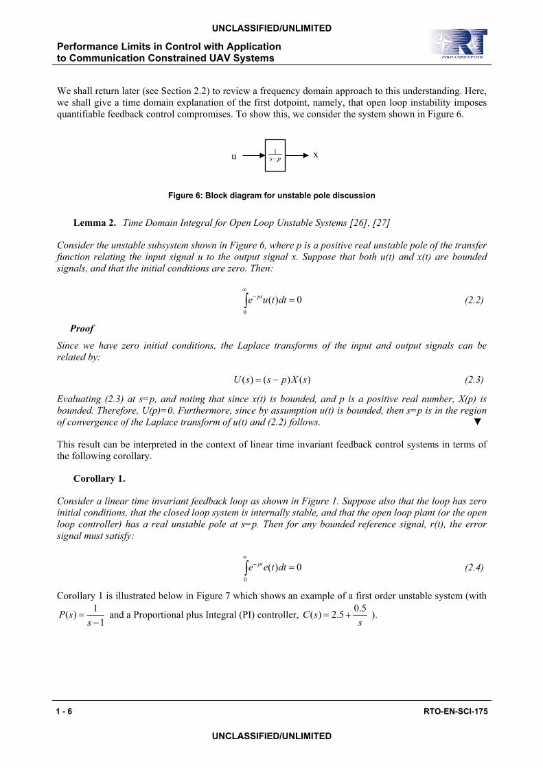
We shall return later (see Section 2.2) to review a frequency domain approach to this understanding. Here, we shall give a time domain explanation of the first dotpoint, namely, that open loop instability imposes quantifiable feedback control compromises. To show this, we consider the system shown in Figure 6.

1s p− x

e x=

u

Figure 6: Block diagram for unstable pole discussion

Lemma 2. Time Domain Integral for Open Loop Unstable Systems [26], [27]

Consider the unstable subsystem shown in Figure 6, where p is a positive real unstable pole of the transfer function relating the input signal u to the output signal x. Suppose that both u(t) and x(t) are bounded signals, and that the initial conditions are zero. Then:

0

( ) 0pte u t dt∞

− =∫ (2.2)

Proof

Since we have zero initial conditions, the Laplace transforms of the input and output signals can be related by:

( ) ( ) ( )U s s p X s= − (2.3)

Evaluating (2.3) at s=p, and noting that since x(t) is bounded, and p is a positive real number, X(p) is bounded. Therefore, U(p)=0. Furthermore, since by assumption u(t) is bounded, then s=p is in the region of convergence of the Laplace transform of u(t) and (2.2) follows.

This result can be interpreted in the context of linear time invariant feedback control systems in terms of the following corollary.

Corollary 1.

Consider a linear time invariant feedback loop as shown in Figure 1. Suppose also that the loop has zero initial conditions, that the closed loop system is internally stable, and that the open loop plant (or the open loop controller) has a real unstable pole at s=p. Then for any bounded reference signal, r(t), the error signal must satisfy:

0

( ) 0pte e t dt∞

− =∫ (2.4)

Corollary 1 is illustrated below in Figure 7 which shows an example of a first order unstable system (with 1( )

1P s

s=

− and a Proportional plus Integral (PI) controller, 0.5( ) 2.5C s

s= + ).





0 1 2 3 4 5-1

-0.5

0

0.5

1

e(t)

CL Step Responses of an open loop unstable system

0 1 2 3 4 5-0.5

0

0.5

1

e(t)

× e-p

t

Time (sec)

Figure 7: Closed Loop Step Response of an example open loop unstable system.

One important consequence of this time domain analysis of open loop unstable systems, is that there is a constraint on the achievable performance (independent of the control design technique) whereby low overshoot demands fast control response. This can be quantified more rigorously as follows. Suppose that we take a non-standard definition1 of rise time, tr as the maximum value for which the following condition, (2.5), holds:

( ) / ; for ry t t t t tr≤ ≤ (2.5)

We also define the overshoot, yos, as the maximum amount by which the closed loop unit step response exceeds unity, max ( ) 1os t

y y t= − . Then under the conditions of Corollary 1, and with the rise time

defined as in (2.5), the closed loop unit step response must have an overshoot that satisfies:

( )1 12

rptr r

osr

pt e ptypt

− +≥ ≥

(2.6)

Note that as discussed in Section 2.1.1, the constraints described above in Lemma 2 and Corollary 1 can be removed in the reference tracking case (that is, a measured exogenous signal) by using a two degree of freedom control structure (or other variants of this, such as nested feedback loops). However, even in these cases, the constraints remain for the response to an output disturbance.

1 Rise time is more often defined in terms such as the time to reach 90% of the final value, or the time to move from 10% to

90% of the final value.





0 1 2 3 4 50

0.5

1

1.5

2

2.5

min yos

tr=0.571

y(t)

0 1 2 3 4 50

0.5

1

1.5min yos

tr=0.25

y(t)

Time (sec)

Figure 8: Closed Loop Step Responses for two different controllers applied to an example open loop unstable system.

Note from Figure 8 that the lower bound on the overshoot given in (2.6) is conservative, and the actual overshoot can be significantly larger. However, it does qualitatively reflect the trade off that it is not possible to have slow rise time and small overshoot in the unity feedback closed loop response of an open loop unstable system.

As an example illustrating the interpretation of this result, we reconsider the NASA X-29 forward swept wing aircraft pitch mode control problem discussed in [25]. There are a range of factors that limit the achievable response speed, with probably the most severe of these being airframe resonance at approximately 7Hz. Because of the uncertainty in this resonance, and the need to ensure control actions do not excite this resonance with the possibility of leading to instability, it could be argued that the control response rise time should be kept to a value no faster2 than 1/7(sec). Also, as reported in [25], the worst case open loop unstable pole is at 6rad/sec in some flight regimes. Combining these results with (2.6) gives a conservative estimate of the achievable unity feedback step response overshoot is 77%. This large value confirms the conclusions of [25], that the constraints on the feedback control system are quite severe, and it is difficult to achieve acceptable closed loop performance. As in [25], this conclusion can be reached without a detailed analysis or design of what controller is to be used.

2.1.3 Plants with Right Half Plane Zeros

Plant zeros in the right half plane are sometimes referred to as non-minimum phase (NMP) zeros of a transfer function, in view of the famous Bode gain-phase relationship [1]. More specifically, the Bode gain-phase relationship is an equality for any stable transfer function with all zeros also in the left half plane. If a transfer function has zeros in the right half plane, then the phase lag is larger than that given by the gain-phase relationship.

To examine the case of plants with non-minimum phase zeros, we first convert these systems into the “zero dynamics form” (see for example [28] for a discussion of this for the case of a nonlinear plant). The

zero dynamics form begins with a linear transfer function model, ( )( ) ( ) ( ) ( )( )

N sY s P s U s U sD s

= = . First, we

2 In [25], in fact it is argued that the bandwidth, “Ω1”, should probably be around 3 rad/sec, which typically would correspond to

a rise time much slower than 1/7 sec.





perform a polynomial division between the numerator and denominator polynomials to produce quotient, and remainder polynomials, Q(s) and R(s):

( ) ( ) ( ) ( )D s Q s N s R s= + (2.7)

Then 1

1 1( ) ( )( )( ) 1 ( ) ( ) (

N s Q sP sD s Q s R s N s

−

− −= =+ )

and we can the turn the original transfer function into the

feedback form illustrated below in Figure 9.

Figure 9: Block diagram transformation from transfer function (a) to zero dynamics form (b) for a linear time invariant system

Note that in the zero dynamics form, the zeros of the original plant transfer function, become poles of the zero dynamics block, Z(s)=R(s)N-1(s), driven by the plant output, y. In particular, note that if the plant is non-minimum phase, that is has right half plane zeros, then the zero dynamics, Z(s), are unstable. It therefore follows, that apart from a change in signal definitions, we have the situation of Lemma 2, which leads directly to Corollary 2.

Corollary 2. Time Domain Integral for Non-minimum Phase Zeros [26], [27]

Consider any control of a plant with a non-minimum phase zero at s=z, where the control results in all signals bounded. Then for zero initial conditions, the plant output, y(t), must satisfy the following time domain integral:

0

( ) 0zte y t dt∞

− =∫ (2.8)

Note that this result can also be understood directly by noting that the left hand side of (2.8) is Y(z), that is, the Laplace transform of y(t) evaluated at s=z. However, with zero initial conditions, Y(s)=P(s)U(s), and under the assumption that both u(t) and y(t) are bounded, U(z) is well defined, P(z)=0 and therefore Y(z)=0.

Figure 10 below illustrates this weighted equal area criterion (2.8), for an example non-minimum phase plant, with a zero at s=+1rad/sec and a PI controller tuned for a slow but low undershoot response.

R(s)N-1(s)

y Q-1(s) u+

u y P(s) -

(a) (b)





0 2 4 6 8 10-0.5

0

0.5

1

y(t)

CL Step Response of a NMP system

0 2 4 6 8 10-0.1

-0.05

0

0.05

0.1

y(t)

× e-z

t

Time (sec)

Figure 10: Illustration of time domain integral for non-minimum phase plants

In the case where we have a real non-minimum phase zero, an immediate consequence of (2.8) is that the output response cannot have a single sign. In particular, if we are considering the step response of a closed loop system, where the plant has a real non-minimum phase zero, then the response must undershoot. Furthermore, the amount of undershoot gets large as a more rapid response time is demanded. This is illustrated in Figure 11 where we see that for fast response times, very large undershoots may occur.

0 2 4 6 8 10-1.5

-1

-0.5

0

0.5

1

y(t)

Time (sec)

Figure 11: Illustration of the response time versus undershoot trade-off for a non-minimum phase plant

The trade-off between response time and undershoot may be made precise by defining the 90% settling time, ts, as the shortest time that satisfies:

( ) 0.9, for sy t t t≥ ≥ (2.9)

In this case, it can be proven (see [26], [27]) that the minimum value of y(t) must satisfy:

1 - 10 RTO-EN-SCI-175




( )0.9 0.9min ( ) for 1

1ssztt

s

y t ztzte

≤ − ≈ −−

(2.10)

More complicated interpretations are available for systems with resonant poles, see for example [30]. In addition, various interpretations of the effects of time delays on the time domain response, and the presence of combinations of time delays, non-minimum phase zeros, and open loop unstable poles can be considered. In such cases, similar analysis can be performed, though the results are more complex to describe and interpret.

We now turn to questions of the analysis of the achievable quadratic performance in some feedback control problems.

2.1.4 Achievable Integral Quadratic Performance

Integral Quadratic performance in control systems has played a very important role as a measure of performance. This is due both to the fact that this type of performance index has proven much more tractable from a mathematical viewpoint, but also, more importantly, because it proves to be a very useful performance measure in many practical applications.

The theory of Linear Quadratic and Linear Quadratic Gaussian control is a very mature field, with classical texts such as [31], [32] available in the field for a long time. These important tools have laid the foundation for more recent techniques in applying optimisation to feedback control problems such as

[33] and Linear Matrix Inequality approaches to optimal control [5]. Here we briefly review some results associated with this area, which help in understanding some limits to the achievable performance. The first of these is known as the minimum energy stabilisation problem, and is based around the setup shown below in Figure 12:

H∞

di

Figure 12: Block diagram of a plant with an input disturbance, di, for consideration of the minimum energy stabilisation problem

Lemma 3. Minimum Energy Stabilisation [31], [34]

Consider a single input, linear, stabilisable plant P(s) with poles at s=pi as in Figure 12. Suppose that with zero initial conditions, the input disturbance is a unit impulse, that is, di(t)=δ(t). Then any stabilising input3, u(t), must satisfy:

(2.11) 2

0

( ) 2i

ip CRHP

u t dt p∞

∈

≥ ∑∫

Furthermore, (2.11) is tight4 if either we have full state feedback, or, we have output feedback and P(s) is both minimum phase and delay free.

3 By ‘stabilising input’ we mean an input that will take all states of P(s) to zero as time tends to infinity.

y+P(s) u +

RTO-EN-SCI-175 1 - 11




Note that Lemma 3 is not intended to be a technique for designing controllers, since the cost function considered is very unrealistic. In particular, there is no cost at all attached to output or state performance (except that there is a requirement for stabilisation) and that often the controllers that result from such an approach have slow response and may have poor robustness properties. However, it does show, in a directly quantifiable form, that open loop unstable systems demand at least a certain minimal amount of control energy, even just to achieve stabilisation.

A closely related problem is the cheap control step response tracking problem depicted in Figure 13.

do

Figure 13: Block diagram of a plant with an output disturbance, do, for consideration of the cheap control tracking problem

In this case, the output disturbance, do, plays a role similar to the reference signal in a tracking problem. The problem is termed ‘cheap control’ since we pay no attention to control energy, provided only that the control energy is finite. Instead, all of our attention is devoted to the energy of the output signal, y(t). We then have the following result.

Lemma 4. Cheap Control Tracking Performance [34], [35], [36]

Consider a single output, linear, stabilisable plant P(s) with zeros at s=zi and time delay τ seconds, as in Figure 13. Suppose that with zero initial conditions, the output disturbance is a unit step, that is, do(t)=1 for t>0. Then for any stabilising input5, y(t), must satisfy:

2

0

1( ) 2iz CRHP i

y t dtz

τ∞

∈

≥ + ∑∫ (2.12)

Furthermore, (2.12) is tight6 if either we have full state feedback, or, we have output feedback and P(s) is open loop stable.

Once again, the cheap control scenario is not intended as a practical control approach, but rather, it indicates succinctly that there is a limit to the output performance that can be achieved. In particular, for non-minimum phase plants or plants with delay the output cannot be both small, and decay rapidly to zero, since this would violate the bound (2.12). These results are useful in showing also that multiple non-minimum phase zeros and time delays do interact and further constrain feedback control performance as compared to considering each component independently. These considerations can also be seen from a frequency domain viewpoint that we now consider.

4 Here ‘tight’ means that there are implementable controllers that achieve stabilisation, and are arbitrarily close to achieving

equality in (2.11). 5 By ‘stabilising input’ we mean an input that will take all states of P(s) to zero as time tends to infinity. 6 Here ‘tight’ means that there are implementable controllers that achieve stabilisation, and are arbitrarily close to achieving

equality in (2.12).

y+P(s) u +

1 - 12 RTO-EN-SCI-175




2.2 A Frequency Domain view of Performance Limitations During the 1980s, Freudenberg and Looze generated a number of extensions and new results based on the work of Bode. The first of these [19] were some key extensions to the Bode sensitivity integral, together with new complex analytic results based on Poisson integrals. In this line of work, the fundamental problem studied is the unity feedback system shown in Figure 1. The key extension to the Bode sensitivity integral is encapsulated in the following result.

Lemma 5. Bode Sensitivity Integral [1], [19]

Consider the linear unity feedback control system depicted in Figure 1, where all signals are scalar. Suppose the closed loop system is internally stable, and that both C(s) and P(s) are proper, and that P(s) is strictly proper. Then:

0

log ( )2

i

ep CRHP

S j d p kω

ω

πω ω π=∞

∈=

⎛ ⎞= −⎜ ⎟⎜ ⎟

⎝ ⎠∑∫ i HF (2.13)

where ip CRHP∈ are the poles of L(s)=C(s)P(s) in the closed right half plane (with units of

radians/sec), and lim ( )HF sk sL

→∞= s .

Note that in the case where the plant has at least 2nd order roll-off at high frequencies (that is relative degree 2), then the high frequency gain is zero, that is, 0HFk = . In this case, by various changes of variables, (2.13) can be re-written as:

0

10( 2 ) 4.343log 10

i i

f

idBp CRHP p CRHPef

S j f df p pπ=∞

∈ ∈=

⎛ ⎞ ⎛ ⎞= ≈⎜ ⎟ ⎜⎜ ⎟ ⎜

⎝ ⎠ ⎝ ⎠∑∫ i ⎟⎟∑ (2.14)

In other words, the net area of the magnitude of the sensitivity function expressed in dB, above and below 0dB, with a linear frequency scale, has to match a scaled sum of the open loop unstable poles. Because the unstable poles always occur in complex conjugate pairs, with positive real parts, the right hand side of (2.14) is always greater or equal to zero. It further indicates that there is a cost associated with pushing for tight performance specifications (small sensitivity, that is very negative values of

dBS ) over a wide range

of frequencies, since this will have to be balanced out by positive values of dBS (that is, disturbance

amplification) at other frequencies.

To illustrate this we consider again the example taken from [25] of the control of the X-29 Aircraft, briefly discussed in Section 2.1.2. This gives a plant transfer function with an unstable pole, at approximately 6 radians per second. In addition, there are a number of system features that enforce plant roll-off from 30 radians per second. We therefore take a very simplified plant model as:

30( )( 6)( 30)

P ss s

=− +

(2.15)

We designed two controllers for the plant in (2.15). The first is a relatively high bandwidth controller, which achieves reasonable sensitivity function performance, and good phase margin (in this case, almost 45degrees, at the gain cross over frequency of 7.73Hz). Unfortunately, this design is impractical for the problem considered, since the aircraft has a lightly damped, difficult to model resonance at approximately 7Hz. Since the loop still has substantial gain at 7Hz, this unmodelled resonance might easily lead to instability. This first design, therefore, does not respect the bandwidth limitations inherent in the system under consideration.

RTO-EN-SCI-175 1 - 13




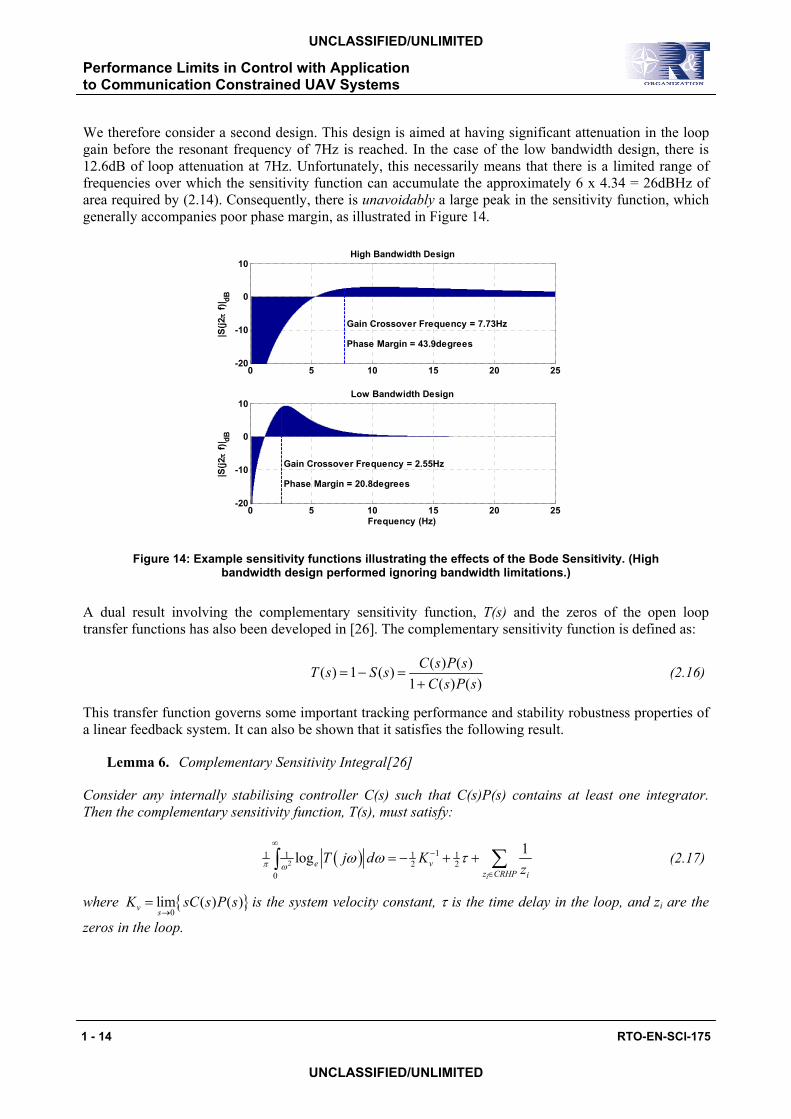
We therefore consider a second design. This design is aimed at having significant attenuation in the loop gain before the resonant frequency of 7Hz is reached. In the case of the low bandwidth design, there is 12.6dB of loop attenuation at 7Hz. Unfortunately, this necessarily means that there is a limited range of frequencies over which the sensitivity function can accumulate the approximately 6 x 4.34 = 26dBHz of area required by (2.14). Consequently, there is unavoidably a large peak in the sensitivity function, which generally accompanies poor phase margin, as illustrated in Figure 14.

0 5 10 15 20 25-20

-10

0

10High Bandwidth Design

Gain Crossover Frequency = 7.73Hz

Phase Margin = 43.9degrees

|S(j2

π f)

| dB

0 5 10 15 20 25-20

-10

0

10

Frequency (Hz)

Low Bandwidth Design

Gain Crossover Frequency = 2.55Hz

Phase Margin = 20.8degrees

|S(j2

π f)

| dB

Figure 14: Example sensitivity functions illustrating the effects of the Bode Sensitivity. (High bandwidth design performed ignoring bandwidth limitations.)

A dual result involving the complementary sensitivity function, T(s) and the zeros of the open loop transfer functions has also been developed in [26]. The complementary sensitivity function is defined as:

( ) ( )( ) 1 ( )1 ( ) (

C s P sT s S sC s P s

= − =+ )

(2.16)

This transfer function governs some important tracking performance and stability robustness properties of a linear feedback system. It can also be shown that it satisfies the following result.

Lemma 6. Complementary Sensitivity Integral[26]

Consider any internally stabilising controller C(s) such that C(s)P(s) contains at least one integrator. Then the complementary sensitivity function, T(s), must satisfy:

( )211 1 1 1

2 20

1logi

e vz CRHP i

T j d Kzπ ω

ω ω τ∞

−

∈

= − + + ∑∫ (2.17)

where 0

lim ( ) ( )v sK sC s P

→= s is the system velocity constant, τ is the time delay in the loop, and zi are the

zeros in the loop.

1 - 14 RTO-EN-SCI-175




As in the case of the Bode Sensitivity Integral (Lemma 5), the Complementary Sensitivity Integral imposes a (weighted) equal area criterion on the log magnitude of T(jω). In this case, the conclusions are

reversed due to the combination of integral action in the loop, and the frequency weighting term, 21

ω, in

(2.17). In particular, for most common loop transfer functions (high gain at low frequencies, low gain at high frequencies), (2.17) can be used to show that the closed loop bandwidth should not be too high compared to the loop time delay and reciprocal of non-minimum phase zeros.

2.3 Extensions Many of the results in the previous two sections were further developed and much of this development is summarised in the research monographs [20], [27], and also articles like the special issue of the IEEE Transactions on Automatic Control [37]. We briefly explore some of the key insights from these works here.

2.3.1 Multivariable Systems

Linear multivariable systems pose some important challenges to the performance limitations analysis expounded earlier. Several additional concepts are essential in these developments. The first of these is to understand some of the issues posed by the non-commutativity of multivariable transfer function matrices. Consider the multivariable feedback loop depicted in Figure 15 where for simplicity, we shall concentrate on the case of ‘square’ multivariable systems, namely, those with equal numbers of inputs and outputs.

Figure 15: Linear Multivariable Unity Feedback Control System

In this case two different loop transfer functions can be identified, namely, the loop transfer function matrix that results if the loop is broken at the input, Li(s)=C(s)P(s), or the loop transfer function matrix if the loop is broken at the output, Lo(s)=P(s)C(s). It is then possible to define two different sensitivity functions, the input and output sensitivities as:

( ) (1( ) ( ) ; ( ) ( )i i o oS s I L s S s I L s ) 1− −= + = + (2.18)

One of the early results for multivariable systems treated them by examining the determinant of the sensitivity function:

Lemma 7. Multivariable determinant Sensitivity Integral[20]

Consider a linear time invariant square strictly proper multivariable system as illustrated in Figure 15. Then:

( ) ( )0 0

log det ( ) log det ( )2

i

e i e o ip CRHP

S j d S j d p kω ω

ω ω

πω ω ω ω π=∞ =∞

∈= =

⎛ ⎞= = ⎜ ⎟⎜ ⎟

⎝ ⎠∑∫ ∫ HF− (2.19)

P(s) C(s) r y +-

e u

dodi

RTO-EN-SCI-175 1 - 15




where lim ( ) lim ( )HF i os sk trace sL s trace sL s

→∞ →∞= = , and pi are the poles of the loop transfer function7.

Note that it can be shown that ( ) ( )log det ( ) log ( )e i e k ik

S j S jω σ= ω∑ and therefore, (2.19) provides

information about the average behaviour of the multivariable sensitivity function, however, it can be difficult to discern from this expression what role the individual components of the multivariable sensitivity function might play.

For simplicity, if we consider multivariable loops with relative degree greater than 1, then it is possible to show (using a simplified, and slightly more conservative, version of the results in [39]) that:

0

0

log ( ) max

log ( ) max

i

i

e i ip CRHP

e o ip CRHP

S j d p

S j d p

ω

ωω

ω

ω ω π

ω ω π

=∞

∈=

=∞

∈=

≥

≥

∫

∫ (2.20)

Tighter results, including a much more detailed explanation of the role of directionality are available in (for example) [39], [27].

We will make use of some basic definitions of directionality to explore extension of the time domain results of section 2.1 to multivariable systems. For simplicity, we assume that the plant, P(s), is a square, generically full rank, transfer function matrix that has distinct and non-repeated poles and transmission zeros. For any zero, s=z define the (output8) zero direction of P(s) at s=z by any unit vector, dz such that

( ) 0Tzd P z = (2.21)

We then have the following result:

Lemma 8. Multivariable Interpolation Constraints [27], [39], [40].

Consider any internally stabilising linear time invariant feedback system. If z is a non-minimum phase zero of P(s) with direction dz, then

( ) 0Tz od T z = (2.22)

where To=I-So is the output complementary sensitivity.

For simplicity, we now consider the error in the response to a step reference change in the 1st element of the reference vector,

1

10

( ) , for 0

0

r t e t

⎡ ⎤⎢ ⎥⎢ ⎥= =⎢ ⎥⎢ ⎥⎣ ⎦

≥

(2.23)

7 Note that provided we maintain internal stability, the CRHP poles of Li(s) and Lo(s) are identical. 8 For our purposes, we shall only discuss explicitly the output directions, so for simplicity we shall simply refer to the direction

vector.

1 - 16 RTO-EN-SCI-175




With this reference signal, denote the output response by

1112

1

( )( )

( )

( )m

y ty t

y t

y t

⎡ ⎤⎢ ⎥⎢ ⎥= ⎢ ⎥⎢ ⎥⎢ ⎥⎣ ⎦

(2.24)

where 11 ( )y t is the response to the step reference, whilst 1 ( ); 2...ky t k m= are interaction or cross coupling

step responses. We then have the following result.

Corollary 3. Multivariable NMP Time Domain Constraint [40]

Consider any internally stabilising, causal multivariable feedback loop. Suppose that the plant, P(s), has a non-minimum phase zero at s=z, with direction [ ]1 2

Tz z z zmd d d d= and suppose also that the first

element, 1zd , is non-zero. Then the response to a reference step in the first element of r(t), (2.23) must satisfy:

11

2 10 0

( ) ( )m

zt ztzkk

k z

de y t dt e y t dtd

∞ ∞− −

=

⎛ ⎞= − ⎜⎜

⎝ ⎠∑∫ ∫ 1 ⎟⎟ (2.25)

Corollary 3 extends the previous single variable result, Corollary 2, by the addition of the extra term on the right hand side of (2.25). Note that these extra terms will be small unless either the direction is not aligned with the first element (that is 1zkd dz ) or the cross couplings ( 1 ( )ky t ) are not small. Note that although the result has been developed for the case where the reference step is in the first element of the reference signal, it clearly also applies (with the appropriate permutations) to a step in any other element. This result and various other interpretations are expounded in [40].

2.3.2 Extensions to Nonlinear Systems

Note that the results above have primarily been explained in terms of linear time invariant systems. It might therefore be questioned as to whether these or similar results apply to nonlinear systems. There are in fact a range of results for nonlinear systems.

The first class of nonlinear system results apply when we have a linear time invariant plant, P(s), but we permit nonlinear (or time varying) controllers, such as that shown in Figure 16.

Figure 16: Linear Discrete Time Plant, P(z), with Nonlinear Control, C(.)

P(z) C(.) r y u

dodi

RTO-EN-SCI-175 1 - 17




Firstly, we note that many of the time domain results apply regardless of the type of control used. For example, Lemma 2 describes an input constraint that applies for plants with an open loop unstable pole, regardless of the type of control However, the interpretation of Corollary 1 do not necessarily apply since this requires expression of the transfer function to the error signal which is not necessarily valid in the nonlinear case. Corollary 2 does however apply since it is expressed directly as an integral constraint on the output signal itself.

The results on achievable quadratic performance of Section 2.1.4 also apply to the case of nonlinear or time varying control of a linear time invariant plant since it is known that linear quadratic control achieves the best possible performance of any causal control. Furthermore, there are several extensions available to the case where the plant itself is non-linear using reduced order nonlinear optimal control problems and the associated Hamilton-Jacobi-Bellman optimal control equations [40], [27].

At first sight, it might seem that there is little hope for extending the frequency domain results, such as the Bode sensitivity integral, to cases that include nonlinear elements. However, there are nonlinear paradigms in which meaningful versions of Bode’s sensitivity integral can be derived.

For example, following the derivations in [41], we consider a Gaussian autoregressive, asymptotically stationary stochastic input disturbance signal, di(t). If we assume:

(i) ‘closed loop stability’; that is, all closed loop signals are asymptotically stationary;

(ii) that the relevant power spectral densities of signals exist;

then we can define a sensitivity function via

( ) ( ) ( )ii u dS ω ω= Φ Φ ω (2.26)

Note that under the assumptions given, except for the trivial case where the noise is zero, the input disturbance, di(t), has a non-singular power spectral density, that is, ( ) 0 for almost all

ud ω ωΦ > . Therefore, the ratio as required in (2.26) is defined for almost all ω.

If we denote the discrete time poles by ihpdip e= (where pi are the continuous time poles), and h is the

sampling period, then we have the following result [41] (for any causal, possibly nonlinear and time varying, control C(.) ):

(2.27) /

0

log ( )i

h

ip CRHP

S d pπ

ω ω π∈

≥ ∑∫ i

Note that the inequality in (2.27) arises since we have only considered the open loop plant unstable poles, whilst the controller might potentially also contribute unstable poles to this expression.

2.4 Caveats, Alternatives, and recent results In the previous subsections, 2.1 to 2.3, we have examined a range of system factors that may limit the feedback control performance. Indeed, from a number of perspectives, these constraints may be loosely translated into the following guidelines:

(a) To stabilise an open loop unstable system requires non-zero control energy. This control action should not have a bandwidth that is slow compared to the unstable poles.

1 - 18 RTO-EN-SCI-175




(b) The control of a non-minimum phase system can be understood in the equivalent form of the plant output driving a feedback version of the unstable zero dynamics. In this form, it can be seen that the permissible outputs are restricted to those that will not de-stabilise the zero dynamics. In particular, high bandwidth (compared to the bandwidth of the zero dynamics) output signals suffer from significant trade-offs due to the requirement to avoid excitation of the unstable zero dynamics.

If these constraints are particularly onerous in a given application, then there are a number of approaches that may be pursued to try to alleviate the limitations.

2.4.1 Alternate Measurements

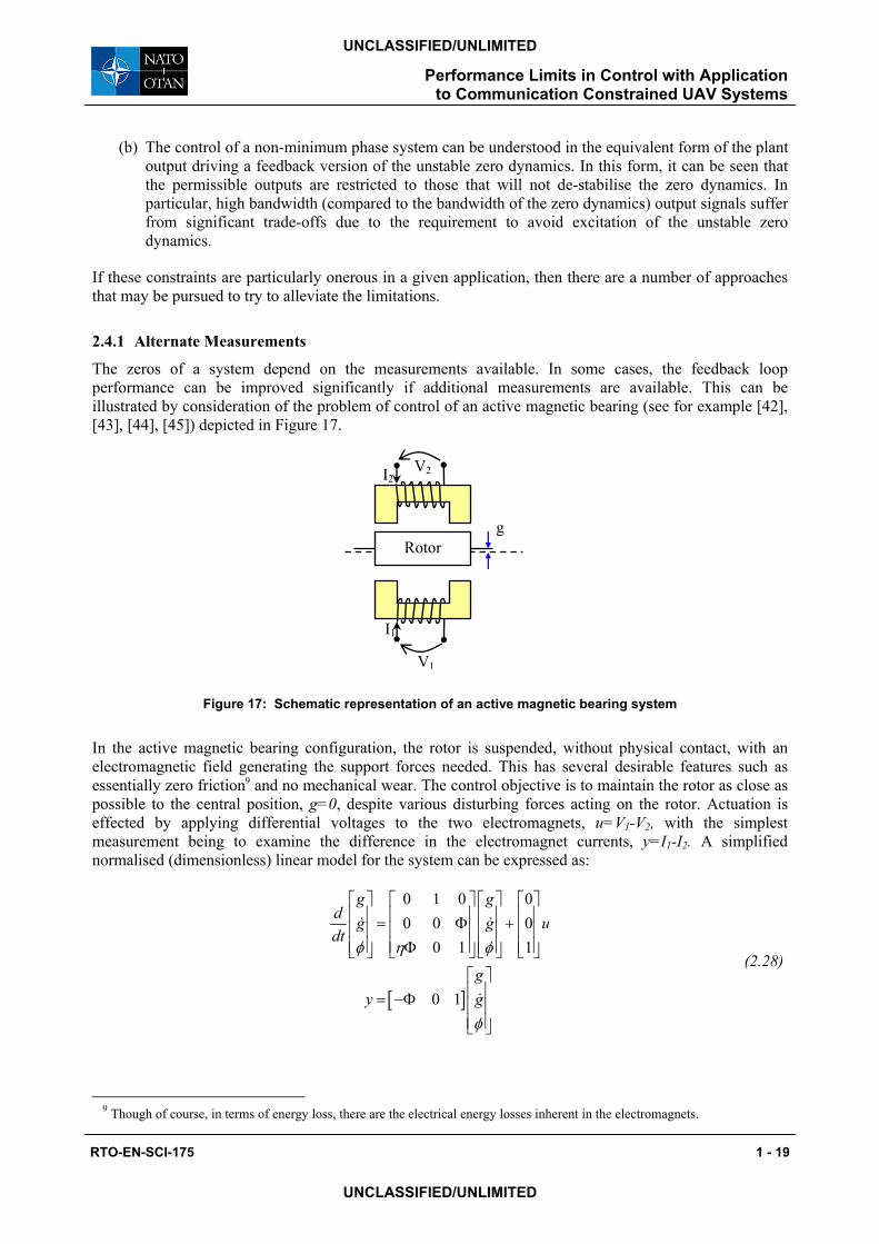
The zeros of a system depend on the measurements available. In some cases, the feedback loop performance can be improved significantly if additional measurements are available. This can be illustrated by consideration of the problem of control of an active magnetic bearing (see for example [42], [43], [44], [45]) depicted in Figure 17.

Figure 17: Schematic representation of an active magnetic bearing system

In the active magnetic bearing configuration, the rotor is suspended, without physical contact, with an electromagnetic field generating the support forces needed. This has several desirable features such as essentially zero friction9 and no mechanical wear. The control objective is to maintain the rotor as close as possible to the central position, g=0, despite various disturbing forces acting on the rotor. Actuation is effected by applying differential voltages to the two electromagnets, u=V1-V2, with the simplest measurement being to examine the difference in the electromagnet currents, y=I1-I2. A simplified normalised (dimensionless) linear model for the system can be expressed as:

[ ]

0 1 0 00 0 0

0 1 1

0 1

g gd g g udt

gy g

φ η φ

φ

⎡ ⎤ ⎡ ⎤ ⎡ ⎤ ⎡ ⎤⎢ ⎥ ⎢ ⎥ ⎢ ⎥ ⎢ ⎥= Φ +⎢ ⎥ ⎢ ⎥ ⎢ ⎥ ⎢ ⎥⎢ ⎥ ⎢ ⎥ ⎢ ⎥ ⎢ ⎥Φ⎣ ⎦ ⎣ ⎦ ⎣ ⎦ ⎣ ⎦

⎡ ⎤⎢ ⎥= −Φ ⎢ ⎥⎢ ⎥⎣ ⎦

(2.28)

9 Though of course, in terms of energy loss, there are the electrical energy losses inherent in the electromagnets.

V1

I1

V2I2

gRotor

RTO-EN-SCI-175 1 - 19




where φ is the (differential) flux in the system, Φ is the (normalised) static flux, and η is the ratio of time constants in the system. This leads to the transfer function:

( )

( )2 2

3 2 2

( )( )( )

sY sP sU s s sη η

− Φ= =

+ − Φ (2.29)

In the case where (using values from practice) Φ=0.288 and η=0.582, the transfer function in (2.29) has an unstable pole at s=0.242 and a non-minimum phase zero at s=0.288. These are located very close to one another, and create substantial difficulties in performing robust control of the system. For example, it is possible to show10 that under these circumstances, the peak sensitivity is always at least 22dB. This is clearly very non-robust, and is unlikely to be implementable in practice.

In practice, it is very natural that measurement of the gap, g, would be used in the controller design. In this case, the transfer function from the control signal, u, to this additional output, g, is given by the minimum phase transfer function:

( )3 2 2

( )( )( )g

G sP sU s s sη η

Φ= =

+ − Φ (2.30)

Whilst this additional measurement does not eliminate the need to consider the unstable open loop pole, it does help alleviate the difficulty associated with controlling a system that is both non-minimum phase and unstable. By combining feedback from both the measurement of the gap and from the current, practical control schemes, without excessive sensitivity peaks can be designed.

As a further note, it is worth pointing out that what is termed ‘sensor-less control’ in the active magnetic bearing community, does not in fact correspond to the equivalent of single input single output linear time invariant control. ‘Sensor-less’ does indicate that the control is performed without a separate physical sensor for position, g. However, despite this, a detailed physical understanding of the magnetics shows that the gap, g, does have a direct impact on the relative inductance seen by the two electromagnets in Figure 17. This difference in relative inductance is directly related to the relative amplitude of high frequency ripple in the two currents, and this can be exploited to create a robust scheme, based on the system nonlinearity, for inferring the position directly from current measurements alone.

2.4.2 Preview Control

Another scheme that may be of advantage in removing some of the limitations in tracking performance due to non-minimum phase zeros is termed ‘preview control’. This scheme relies on having measured external signals (such as the reference command to be tracked) where there is also advance knowledge of future signals. This may be a realistic scenario, for example, for some path tracking scenarios, such as in robotics; or terrain following for an aircraft.

Several early works (for example [46], [47]) related to this area studied problems of ‘nonlinear system inversion’ for non-minimum phase systems. Nonlinear systems inversion is the problem of generating the input signals for a system that will cause the output to follow a specified path. This problem is well studied, and in the case where the inverse system is stable, that is, when the zero dynamics are stable, the solutions are straightforward. Where the zero dynamics are not stable, more complex analysis is needed to permit inversion. In particular, if the target output has been pre-specified for all time, it is possible to use this information to generate a control trajectory that will cause the output to follow the target trajectory.

10 This can be established using, for example, the Poisson Sensitivity Integral [19], [27].

1 - 20 RTO-EN-SCI-175




In a feedback control context, this approach can be understood via the block diagram given below in Figure 18.

Time Advance

r uH

Figure 18: Preview Control block diagram

Note from Figure 18 that the preview control approach includes both a conventional feedback path with controller C(s) together with a reference feed-forward path, with feed-forward compensator HFF(s). This is the common two degree of freedom control structure. However, it can be shown that the two degree of freedom control structure does not, of itself, eliminate the constraints on output performance due to unstable zeros. The key to the advantage of preview control is the ‘anti-causal’ (time advance) block whereby advance knowledge of future reference signals, r(t+T), is able to be utilised immediately to generate the reference feed-forward signal, uH(t). The potential improvement in performance is illustrated in Figure 19. In Figure 19(a) we illustrate the potential performance when control without preview is used. Here, the constraints described in Section 2.1.3 apply whether or not we use a two degree of freedom control structure. However, as illustrated in Figure 19(b), the use of preview allows the control to take some initial corrective actions, which ‘prepare’ the system for the rapid trajectory change that occurs at t=4 seconds.

Figure 19: Preview Control Example: (a) Example Step Reference Responses without Preview; (b) Example Step response with four second preview.

(b) (a)

P(s) C(s) ye=r-y

HFF(s) r(•)

uC

-

e+sT r(t+T)

RTO-EN-SCI-175 1 - 21




2.4.3 Path Tracking

“Path Tracking” describes an alternate control paradigm that may be relevant in a range of situations, such as when controlling a numerically controlled machine to cut a work-piece; some grinding operations, terrain following in an aircraft. In this paradigm, the control objective is not to make the output, y(t), track a reference signal, r(t) which is specified for all time. Instead, the objective is to make the output, at every instant in time, be close to a pre-specified path. This is illustrated below for the case of a two dimensional output vector in Figure 20

y(t)y2

r

r(t)y1

r(θ(t))

Figure 20: 2-D Diagram depicting the difference between regular feedback control tracking where the relevant performance variable is e(t)=r(t)-y(t) and path tracking where ep(t)=r(θ(t))-y(t).

There is therefore considerable freedom in how to select the ‘timing’ function, θ(t), so that improved performance may result. In particular, if the output response is constrained due to non-minimum phase zeros, then the constraints in Sections 2.1.3 and 2.1.4 will apply in the normal case. This is also true in the case of path tracking, except that if we can design the timing function appropriately, then the restriction may disappear. In particular, suppose that we have a NMP zero at s=z, with direction, dz (as discussed in Section 2.3.1), then if we can achieve a selection of θ(t) such that ( ) 0T

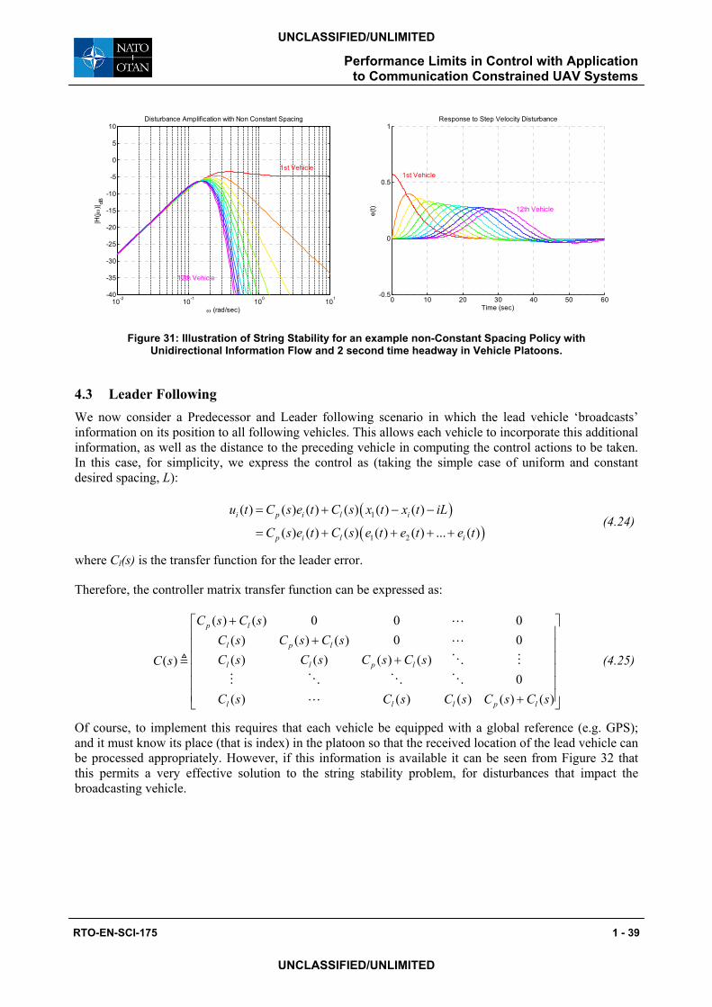
z pd R z = it will be possible to achieve very small tracking errors, without destabilising the unstable zero dynamics. Situations where this is possible and techniques for designing (at least in an ideal setting) suitable θ(t) are discussed in (for example) [49], [50].

3.0 PERFORMANCE LIMITATIONS AND COMMUNICATION CONSTRAINTS

We now turn to discuss a different aspect of performance limitations in feedback loops, namely communication constraints. There has recently been a great deal of research interest in studying this class of problems. This has in part been generated by the increasing demand for systems without dedicated wiring to individual sensors, but rather making much greater use of modern communication networks. In addition to this, problems involving wireless sensors increase the complexity of problems that may be faced by modern feedback control systems. These problems, often based around tight real time constraints, are not always well supported by the communications network protocols, and therefore need additional attention in the control design.

1 - 22 RTO-EN-SCI-175




3.1 Control over Communications Systems

Plant Plant

Figure 21: Traditional control (a) versus control over communications (b) scenarios.

The control over communications scenario commonly studied diverges from the traditional control approach of Figure 21(a) where all communication links are ‘perfect’ and replaces it by the scenario shown in Figure 21(b) where (at least some of) the links are analysed as being ‘imperfect’. Some of the different imperfections that have been studied in the literature include:

• Variable transmission delays [6]. For example, if TCP or similar protocols are used in the communications, the network delay is variable, and can exhibit long tail distributions.

• Occasional errors [7]. For example, if the network is very congested, then the original data may not be received, despite repeated retries. In some cases, if the communications protocol includes an acknowledgement (‘ACK’), then if the ‘ACK’ gets lost in the network, the original data may be retransmitted, even though it has already been received.

• Signal quantisation [8], [9], [10], [11] is often considered amongst the consequences of digital communications in feedback control systems.

• Signal bandwidth [12], and data rate limits [13], [14], [15], [16], [17] are also important factors in some communication systems. These will be particularly relevant if wireless communication is employed and where there is a large number of information connections required.

3.2 Information Theoretic Properties One of the fundamental issues in the control over communications setting (and indeed, to some extent, this is inherent in other scenarios, such as finite relative precision sensors) is the need to understand information and information flow properties and their impact on feedback control. Information Theory has been studied extensively in the communications context, however, control with a much deeper requirement for real time and feedback (that is, correlated) properties in such systems have been more difficult to analyse. We now briefly review some key information theoretic concepts and properties. These follow standard information theory texts such as [51] and have been used in recent works on control over communications including [14].

3.2.1 Entropy of a Random Variable

The Entropy (HX) of a Discrete Random Variable (X) is defined by11:

( ) 2: log ( )H X E p X= − (3.1)

11 Note that the Entropy is often defined in terms of the natural logarithm, in which case it is sometimes said to have units of

‘nats’, rather than the base 2 case, where the units are ‘bits’.

Controller Communication

Channel Decoder Encoder

Controller (Pre)

Controller (Post)

(a) (b)

RTO-EN-SCI-175 1 - 23




It can be loosely though of as the number of binary bits required to represent the information in X. For example, if X is an unbiased coin toss, with two equally probable outcomes, then H(X)=1. If X is a deterministic variable, that is, there is only one possible outcome, then H(X)=0.

For a random variables with a continuous distribution, f(x), the continuous or differential entropy is defined as:

(3.2) 2( ) ( ) log ( )H X f x f x dx= ∫For example, a scalar Gaussian random variable with mean µ, and variance, σ2 the (continuous) entropy is can be calculated as:

( )

( )( )

2 2

2

2

2( ) 22

2

22

2

( ) ( ) log ( )

log ( ) ln( 2 )22

1 ln( 2 ) ; with ( ) /2ln 2 2

log 2

x

y

H X f x f x dx

e xe d

ye dy y

e

µ σ µ σ πσσ π

x

xσ π µπ

σ π

∞− −

−∞

∞−

−∞

= −

⎛ ⎞−= − − −⎜ ⎟

⎝ ⎠⎛ ⎞

= + =⎜ ⎟⎝ ⎠

=

∫

∫

∫ σ−

(3.3)

In this case, we see from (3.3) that the entropy is directly related to the logarithm of the variance. In the case of a multivariate Gaussian of dimension n, with covariance ΣX has entropy

( ) ( )(2( ) log 2 detnXH X eπ= )Σ . This is directly proportional to the logarithm of the ‘effective’ volume

of support of the multivariable distribution - ( )det XΣ .

The definitions of Entropy permit directly definition of the Entropy Power N(X) of an n dimensional random variable, X as

2 ( ) /1( ) 22

H X nN Xeπ

= (3.4)

Following (3.3), and the following equations, for a multivariate Gaussian, with covariance Σx, the entropy power is:

( )1

( ) det nXN X = Σ (3.5)

The entropy power satisfies some important properties. Firstly, it is known that it is a lower bound on the variance, that is regardless of whether a random variable is Gaussian or not: ( )TE X X nN X⎡ ⎤ ≥⎣ ⎦ (3.6)

Also, it turns out that the entropy power is super-additive, that is, for any two independent random variables, X,Y:

( ) ( ) ( )N X Y N X N Y+ ≥ + (3.7)

1 - 24 RTO-EN-SCI-175




3.2.2 Mutual Information and Capacity

These definitions of Entropy (and Entropy power) translate immediately to the conditional Entropy of a random variable conditioned on another random variable, e.g. H(X|Y) is the conditional entropy of X given Y. From these definitions, the mutual information between two random variables, X,Y can be defined as:

(3.8) ( ; ) ( ) ( | ) ( ) ( | )I X Y H X H X Y H Y H Y X= − = −

Apart from the desirable symmetry property, this definition of mutual information also has the property that if X,Y are independent, then their mutual information is zero, since H(X|Y)=H(X). In addition, if X,Y are completely determined by one another (for example, X=Y), then the mutual information is I(X;Y)=H(X).

It is generally the case, that a communication channel has limits on the rate at which it can transfer information. This can be defined more formally as a limiting case of a channel with input X and output Y. Denote by XT and YT the total information in X and Y over the interval [0,T]. Then the channel capacity, C, is defined as the supremal average rate of information flow:

1sup lim ( , )T

T TTTXI X Y

→∞=C (3.9)

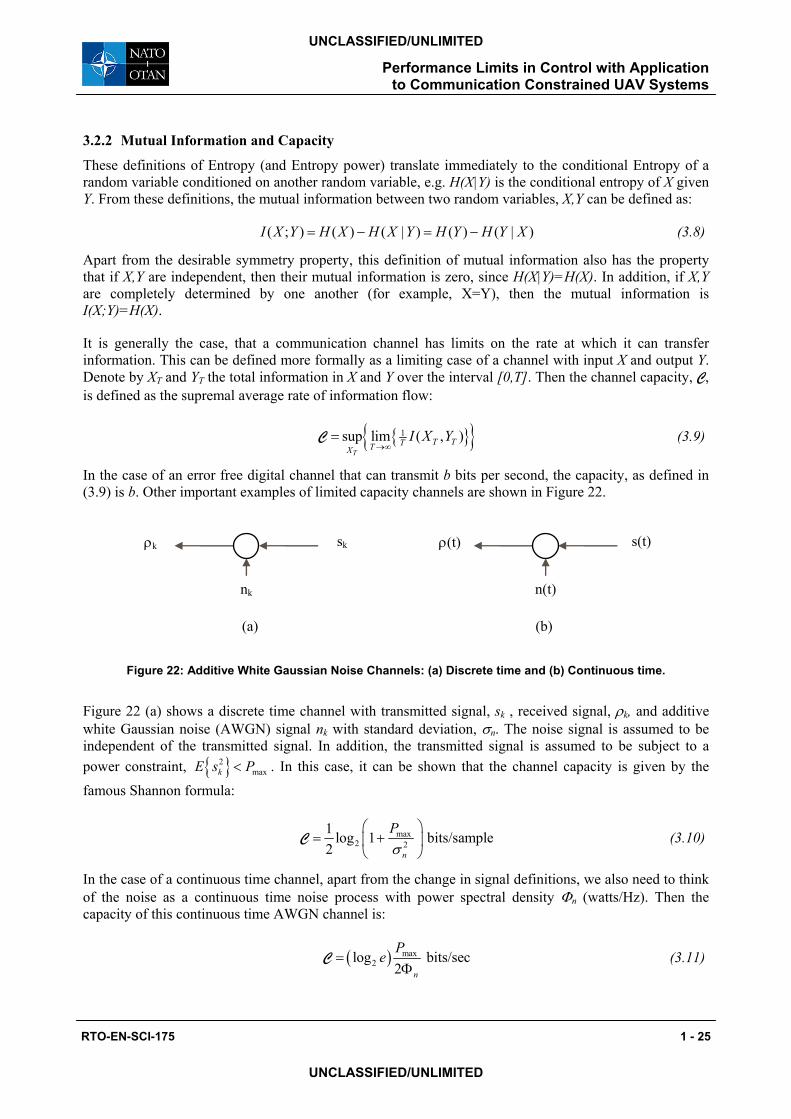
In the case of an error free digital channel that can transmit b bits per second, the capacity, as defined in (3.9) is b. Other important examples of limited capacity channels are shown in Figure 22.

Figure 22: Additive White Gaussian Noise Channels: (a) Discrete time and (b) Continuous time.

Figure 22 (a) shows a discrete time channel with transmitted signal, sk , received signal, ρk, and additive white Gaussian noise (AWGN) signal nk with standard deviation, σn. The noise signal is assumed to be independent of the transmitted signal. In addition, the transmitted signal is assumed to be subject to a power constraint, 2

maxkE s P< . In this case, it can be shown that the channel capacity is given by the

famous Shannon formula:

max2 2

1 log 1 bits/sample2 n

Pσ

⎛ ⎞= +⎜ ⎟

⎝ ⎠C (3.10)

In the case of a continuous time channel, apart from the change in signal definitions, we also need to think of the noise as a continuous time noise process with power spectral density Φn (watts/Hz). Then the capacity of this continuous time AWGN channel is:

( ) max2log bits/sec

2 n

Pe=Φ

C (3.11)

nk

(a) (b)

skρk s(t) ρ(t)

n(t)

RTO-EN-SCI-175 1 - 25




We now turn to discuss some fundamental implications of information constraints, that is, limited capacity communication, on feedback control performance.

3.3 Information Constrained Control

3.3.1 Capacity Required for Stabilisation [14], [52]

Consider a linear time invariant discrete time plant represented by the state space equation:

1k k kx Ax Bu+ = + (3.12)

In particular, we consider the case where the plant is open loop unstable, that is some of the eigenvalues of A are outside the unit circle. We then perform a state transformation into stable and unstable subspaces, so that (3.12) is becomes:

1

1

00

u uu uk k

ks ssk k

x xAu

x xA B+

+

⎡ ⎤ ⎡ ⎤s

B⎡ ⎤ ⎡ ⎤= +⎢ ⎥ ⎢ ⎥⎢ ⎥ ⎢ ⎥

⎣ ⎦ ⎣ ⎦⎣ ⎦ ⎣ ⎦ (3.13)

where all eigenvalues of Au are (strictly) outside the unit circle, and all eigenvalues of As are on or inside the unit circle. We denote by ρk the signal received by the communication channel, where the transmitted signal sk is permitted to be any signal causally related to the plant state. We also define by nk the entropy power of u

kx conditioned on the information in all past received signals, Rk=ρk-1, ρk-2, …,ρ0:

( ) |u kk kn E N x R= (3.14)

Then it follows (after some analysis, see for example [14], [52] ) that nk satisfies the recursion:

( )2 22

1 2 2u un nnk kn A n A

⎛ ⎞−⎜ ⎟ −⎝ ⎠+ ≥ =

CC

kn (3.15)

From (3.15) it is clear that a necessary condition for nk to not diverge is that 2uA − <C 1, or equivalently, a

necessary condition for stabilisation is that:

2log bits/sampleui

iφ⎛ ⎞

> ⎜ ⎟⎝ ⎠∑C (3.16)

where uiφ are the eigenvalues of Au. In the case where the discrete time system is based on a sampled

version of a continuous time system, with unstable (that is, right half plane) eigenvalues pi, then (3.16) can be rewritten as:

(3.17) ( )2log bits/secondii

e p⎛ ⎞> ⎜ ⎟

⎝ ⎠∑C

Note that (3.16) gives a fundamental communication capacity limit required for any limited capacity causal feedback loop to be able to stabilise the system (3.13).

1 - 26 RTO-EN-SCI-175




3.3.2 Capacity Required for Performance [53], [52]

Note that the results of Section 3.3 can be generalised to include some stochastic measures of performance, as in the following results. Suppose that the plant equation includes a stochastic disturbance term, vk, as follows:

1

1

00

u uu uk k

k

uk

s ss sk k

sk

x xA Bu

vx x vA B

+

+

⎡ ⎤ ⎡ ⎤ ⎡⎡ ⎤ ⎡ ⎤= +⎢ ⎥ ⎢ ⎥ ⎢⎢ ⎥ ⎢ ⎥

⎣ ⎦ ⎣ ⎦⎣ ⎦ ⎣ ⎦ ⎣

⎤+ ⎥

⎦

uk

(3.18)

In this case, the dynamics of the unstable portion of the dynamics can be written as

1u u u uk k kx A x B u v+ = + + (3.19)

Then, the equivalent of (3.15) becomes:

(2 12

1 2 det uu n nn

k k vn A n

⎛ ⎞−⎜ ⎟⎝ ⎠

+ ≥ +C )Σ (3.20)

which directly leads to

( )

1

22

detliminf

1 2

un

vkk

u nn

nA

⎛ ⎞→∞ −⎜ ⎟⎝ ⎠

Σ≥

−C

(3.21)

Therefore, in view of (3.6), it follows that there is a lower bound on the achievable performance of the system for any causal, but limited capacity feedback

( )1

2

222

detliminf

1 2

un

vukk

u nn

E x nA

⎛ ⎞→∞ −⎜ ⎟⎝ ⎠

Σ≥

−C

(3.22)

In the case where we have a scalar unstable system, that is, the dimension, n, of xu is 1, then (3.22) simplified to:

( ) ( )( )2 2

2 2

1liminf1 2

ukk

E x vσφ −→∞

≥− C

(3.23)

where φ is the (scalar) unstable pole, and 2vσ is the variance of the process noise. In this case, we see that

there is a lower bound, based on the capacity of the feedback channel, on the disturbance amplification. Furthermore, as the capacity approaches the limit required for stabilisation (in this case, C→log2|φ|) the disturbance amplification grows without bound.

3.4 Signal to Noise Ratio Constrained Control The lower bounds in (3.16) and (3.23) have been shown to be tight in the case of an error free bit rate limited channel (see for example [14], [53]). In this section, we also investigate this problem from the perspective of signal to noise ratio limited control [52].

RTO-EN-SCI-175 1 - 27




P(z)

Figure 23: Linear discrete time control over a signal to noise ratio constrained channel

In Figure 23, we allow both K1(z) and K2(z) to be used as controllers or compensators for the channel.

3.4.1 SNR constrained Stabilisation

For simplicity, we consider the case of state feedback, and where the plant is antistable12, that is, completely unstable. In this case, we have the following result.

Lemma 9. State Feedback Stabilisability over an SNR Limited AWGN Channel

Consider a discrete time plant with unstable poles at z=φi and an additive white Gaussian noise channel, where the noise, nk, has variance σk, and the transmitted signal has power limit 2

maxkE s P< . Then with

state feedback, the plant can be stabilised if and only if

2max2 | | 1i

in

Pφ

σ⎛ ⎞

> ⎜ ⎟⎝ ⎠∏ −

2n

(3.24)

Proof:

The necessity of (3.24) follows from (3.16) together with the expression for the capacity of an AWGN channel,(3.10). The sufficiency of (3.24) can be established constructively as follows. Set K2(z)=-1, and then design a minimum energy stabilising state feedback KME. If we then set K1(z)=KME then clearly we have a stabilising state feedback gain. It remains to verify that this state feedback gain gives a closed loop system that satisfies the power constraint. It can be established, see for example [52], that this minimum energy stabilisation scheme achieves transmitted signal energy:

2 2| | 1k ii

E s φ σ⎛ ⎞⎛ ⎞

= −⎜⎜ ⎟⎝ ⎠⎝ ⎠∏ ⎟ (3.25)

The result of Lemma 9 has been derived for the case of state feedback, however, there are also variations of this that apply to the output feedback case.

Corollary 4. Output Feedback Stabilisability over an SNR Limited AWGN Channel [52]

Consider a discrete time plant that is minimum phase and relative degree one with unstable poles at z=φi and an additive white Gaussian noise channel, where the noise, nk, has variance σk, and the transmitted signal has power limit 2

maxkE s P< . Then with output feedback, the plant can be stabilised if and only if

12 Note that the case where the plant includes both stable and unstable poles follows in a similar fashion by performing a

decomposition into stable and unstable components. There are some extra technical difficulties when the plant includes marginally stable poles, but it turns out that these do not alter the capacity required for stabilisation.

K1(z) K2(z)

rk sk

nk

1 - 28 RTO-EN-SCI-175




2max2 | | 1i

in

Pφ

σ⎛ ⎞

> ⎜ ⎟⎝ ⎠∏ −

kv

(3.26)

Note however, that in cases where the plant has relative degree greater than unity or has non-minimum phase zeros, the situation is less clear, and linear time invariant compensators will not in general achieve a tight bound such as that in (3.26).

3.4.2 SNR constrained Performance

When considering the performance question posed along similar lines to that in Section 3.3.2, the signal to noise ratio constrained framework is very convenient, since it is equivalent to a decentralised or cooperative linear quadratic Gaussian control problem. This can be seen by considering K1(z) and K2(z) as two different ‘agents’, with limited information transfer, trying to achieve the transmitted power constraint, whilst simultaneously achieving some level of plant performance. In their most general form, such problems are known to be potentially non-convex, and the Witsenhausen counter-example [54] shows that nonlinear compensation can indeed outperform linear compensators in some cases.

However, as recently observed by Rantzer [55] there are results (e.g. [56]) that some classes of decentralised LQG problems are indeed convex, and admit linear time invariant controllers that achieve optimal performance.

One simple case where we are able to establish tight results is the case of scalar unstable dynamics driven by an additive disturbance, which we simplify to:

1k k ky y uφ+ = + + (3.27)

In this simple case, it turns out that linear time invariant compensation does achieve the bound given in (3.23). In particular suppose vk is a white noise sequence of variance 2

vσ , and we take static linear feedback gains as defined in (3.28)

( )( )

( ) ( )( )

2 2max max

1 2max

max2 2 2

max max

11( )

( )1

n

v n

vn n

P PK z

P

PK zP P

φ σ

σ σ

σ φ2σ φ σ

+ −=

+

=+ + −

(3.28)

Then it can be shown that these are stabilising gains that achieve the bound, 2maxkE s P= , and that give:

( )( )( )

( )( )

2max2 2

max2 2 21 max

212 2

max

11

1

1 1

nk v

n

v

n

PE y P

K P

P

σσ

φ σ

σφ σ

−

+→ =

+ −

=− +

(3.29)

Note that (3.29) reduces to the bound on the achievable performance, (3.23), on using the expression for the capacity of an AWGN channel, (3.10).

RTO-EN-SCI-175 1 - 29




3.4.3 Generalisations of Bode’s Integral Theorem [41]

More recently, there have been some significant advances made in linking together Bode’s Sensitivity Integral, Lemma 5, with information theoretic concepts. This work starts by considering the configuration shown in Figure 24.

v

Figure 24: Loop set up for Generalised Bode integral discussions

In this figure, the encoder and decoder are allowed to be any causal operators, that is, they are permitted to be nonlinear or time varying, and the channel is permitted to be a digital channel, or a power limited noise corrupted channel, with limited capacity. In this context, we follow the development in Section 2.3.2, where the disturbance, vk, is assumed to be a stationary, Gaussian, moving average process, and therefore has a well defined power spectral density Φv(ω). We also assume that the sequence, uk, is asymptotically stationary, and admits a well defined power spectral density, Φu(ω). Recall then that we define a sensitivity like function Si(ω) as follows:

( )( )( )

ui

v

S ωω

ωΦ

=Φ

(3.30)

The result in (2.27) can be extended to include explicitly the impact of communication capacity limitations in the following Lemma.

Lemma 10. Bode like Sensitivity Integral (Impact of Feedback Capacity Limitations)[41]

Under the same conditions as in Section 2.3.2 and in addition, with feedback of limited capacity C. Then:

/

0

1 min 0,log ( )i

h

ip CRHP

S d pπ

ω ωπ ∈

⎛ ⎞≥ ⎜ ⎟⎜ ⎟

⎝ ⎠∑∫ Ci − (3.31)

Note that the term min 0,log ( )iS ω in Lemma 10 is always non-positive. In fact, it is the negative of the log sensitivity reduction at the frequency ω, or zero if there is no sensitivity reduction. Therefore Lemma 10 can be loosely interpreted as saying that the net area of log sensitivity reduction is equal to

i

ip CRHP

p∈

⎛ ⎞− ⎜⎜

⎝ ⎠∑C ⎟⎟ . In particular, if this term is negative, then stabilisation is not possible. Furthermore,

sensitivity reduction of a significant size and bandwidth is not possible without sufficient additional capacity.

P(z) uC(.) y

Channel Decoder Encoder

1 - 30 RTO-EN-SCI-175




The implications of this are shown below in Figure 25. This shows three different sensitivity functions achieved for different feedback channel capacities. In each case, the plant is the simple discrete time

unstable plant, 1( )1

P zz

=−

, and the controller is designed to make the received signal, ρk, white13.

0 0.1 0.2 0.3 0.4 0.5-15

-10

-5

0

5|Si(ω)|dB versus capacity

F

5.0bps2.0bps1.0bps0.5bps

Figure 25: Example ‘Sensitivity’ Functions for different feedback capacities.

4.0 APPLICATIONS TO DISTRIBUTED SYSTEMS & FORMATION CONTROL

In the context of this paper, distributed control systems are characterised by:

•

•

•

Large numbers of interacting systems

Limited communication connectivity between subsystems

Limited Communication rates between subsystems.

Control of distributed systems involves a range of issues beyond those analysed in the previous two sections. In addition to there being a range of multivariable dynamic feedback systems with communication constraints, there are particular communication structures within the network that may be important. Issues related to distributed systems have also been studied under the closely related fields of decentralised control (though in this case, this is sometimes more directed at systems with comparatively weak interactions), or, coordinated, cooperative or consensus control.

Arguably one of the simplest forms of distributed control to consider is one dimensional problems, including the control of ‘strings’. This has a long history, including early works describing a problem known as ‘string stability’ (see for example [57], [58]; or [59] for more recent work) that has been discussed in relation to vehicle platooning in automated highway systems. The setup considered in this context is depicted in Figure 26 below.

13 This choice is designed to improve the utilisation of the channel.

RTO-EN-SCI-175 1 - 31




3 2 n 1

X xn x3 x2 x1

Figure 26: Vehicle Platooning schematic: n vehicles travelling in the positive X direction

In Figure 26, we consider a set of n vehicles, all travelling in the positive X direction, with positions denoted by xi and velocities denoted by vi. For simplicity, we take a control algorithm that is effectively a velocity actuator, and therefore our model of the vehicles themselves, when suitably normalised, is:

i ix u= (4.1)

The control objective for the first vehicle is to track a desired ramp trajectory, r(t). We therefore define the error variable for the first vehicle as:

1( ) ( ) ( )e t r t x t1= − (4.2)

Then, using (4.1) in (4.2) we obtain the error variable model:

(4.3) 1 1 1( ) ( ) ( ) ( ) ( )e t r t u t d t u t= − − 1

For the remaining vehicles, the control objective is to make each of the inter-vehicle spacings equal to14 a desired value, Li, (which may depend on the position and velocity of the vehicle), and in addition, follow the lead vehicle’s velocity, v1. Therefore, we can define the error as:

( )1 ; 2,3,...,i i i ie x x L i−= − − = n (4.4)

Then combining (4.4) with (4.1) we obtain the dynamic equation in error coordinates as:

1 ; 1... 1i i i ie u u L i n−= − − = − (4.5)

To minimise this error, given complete information is a fairly straightforward control problem. However, in practice, there may be a heavy cost involved in transmitting control information between widely separated vehicles in the platoon. Therefore, there has been considerable interest in controllers that rely on very limited information. However, it turns out that this can easily lead to a problem known as string instability.

4.1 String Instability

4.1.1 Unidrectional Information, Constant Spacing Policy

In the case of unidirectional information flow, we assume that the local controller for vehicle i only has access to the error in position to the vehicle in front. In other words, controller i only has access to ei. If in addition, we have a constant spacing policy, then L is constant, and therefore the second derivative term in (4.5) disappears. Under these assumptions, the effective feedback control block diagram can be illustrated in Figure 27.

14 In fact, in practice, it may be sufficient to ensure a minimum inter-vehicle spacing. However, for efficiency reasons, we do not usually wish to have inter-vehicle spacing too large either, and so here we take this as a regulation problem.

1 - 32 RTO-EN-SCI-175




Figure 27: Vehicle Platooning control block diagram: Unidrectional information, and constant spacing policy.

With the control structure as shown in Figure 27 define the complementary sensitivity function for section

i, as ( )

( )( )

ii

i

C sT s

s C s=

+. Then the overall transfer function from d1 to the final error signal, en can be derived

as:

1

1 1 21

1 1 1( ) ( )( ) ( ) ( )

n

n n n n iin n n

e u T s u Ts C s s C s s C s

−

− − −=

⎛ ⎞ ⎛ ⎞ ⎛ ⎞⎛ ⎞= ∗ = ∗ =⎜ ⎟ ⎜ ⎟ ⎜ ⎟⎜ ⎟+ + + ⎝ ⎠⎝ ⎠ ⎝ ⎠ ⎝ ⎠

∏ 1s d∗ (4.6)

It can be shown (see for example [57], [58], [59]), that this configuration leads to a problem known as ‘string instability’. This is illustrated in the simulations shown below in Figure 28 where each controller is

taken to be a simple proportional plus derivative controller, with transfer function ( )1.25 0.25( )i

sC s

s+

= ,

designed to keep small overshoot and small ‘amplification’ in sup ( )T jω

ω , at the expense of relatively

long settling time.

10-1 100 101-40

-35

-30

-25

-20

-15

-10

-5

0

5

10

ω (rad/sec)

|H(j ω

)| dB

Disturbance Amplification versus position

1st Vehicle

12th Vehicle

0 5 10 15 20 25 30 35 40-0.5

0

0.5

1

1.5

Time (sec)

e(t)

Response to Step Velocity Disturbance

1st Vehicle

12th Vehicle

Figure 28: Illustration of String Instability for an example Constant Spacing Policy with Unidirectional Information Flow in Vehicle Platoons.

A key question that might arise in this context is whether or not the string instability behaviour illustrated in Figure 28 is a consequence of poor controller choice, or whether it is inherent to the configuration. A simplified view of this, which ignores some of the subtleties in the definitions of l2 versus l∞ string stability is to use the frequency response definitions and a variant of Lemma 6. To this end, define

- - +

e1

1s

C1(s)

d1u1 +

e2

1s

C2(s)

u2+ -

1s

en

Cn(s)

un

RTO-EN-SCI-175 1 - 33




1

1,11

( ) ( )n

ni

T s T s−

−=

= ∏ i and note that from (4.6) that to keep en well behaved in response to a disturbance in the

lead vehicle, d1, we need Tn-1,1(s) to be well behaved as n grows. It turns out that under the conditions posed, and assuming the controllers incorporate integral action, are delay free and minimum phase15; that Tn-1,1(s) satisfies an equation directly equivalent to (2.17):

( )21

1,10

log 0e nT j dω

ω ω∞

− =∫ (4.7)

We then have the following result that establishes unbounded growth in sup ( )T jω

ω under some fairly

mild assumptions about the low and high frequency response:

Lemma 11. String Instability

Suppose that the individual closed loop transfer functions in the string are type II systems and satisfy the following two conditions:

(i) High Frequency Roll-off condition. There exists an angular frequency, ωh>0 such that

( ) ; for all , 1... 1hi hT j i nω

ω ω ωω

≤ > = − (4.8)

(ii) Low Frequency response. There exists an ε>0 and an angular frequency, ωl< ωh , such that

2( ) 1 ; for all , 1... 1iT j i nω εω ω ω≤ + < = −l (4.9)

Then, the peak value of 1,1sup ( )nT jω

ω− grows without bound with n.

Proof

Without loss of generality, take 1l

h

ωεω

< since if this is not the case, we simply chose a smaller ωl until it

is true. Then by splitting the interval of integration in (4.7) we have

( ) ( ) ( )

( ) ( )

( )

2 2 2

2 2

1 11 1 1

1,11 10

21 1

0

log log log

1 log 1 log

11

h l

l h

l

h

n n

e n e i e ii i

he e

lh

T j d T j d T j d

n d

n

ω ω

ω ω ωω ω

ω

ω ωω

d

ω ω ω ω

ω

ω ω

εω ω ωω

εωω

∞− −

−= =

∞

⎡ ⎤≥ − −⎢ ⎥

⎢ ⎥⎣ ⎦⎡ ⎤⎛ ⎞≥ − − + −⎢ ⎥⎜ ⎟

⎝ ⎠⎢ ⎥⎣ ⎦⎡ ⎤

≥ − − +⎢ ⎥⎣ ⎦

∑ ∑∫ ∫ ∫

∫ ∫ (4.10)

Clearly from (4.10) [ ]

( ) ( ) 21,1,

max log 1l

l h

le n

h

T j nω ω ω

ωω εω

ω−∈

⎡ ⎤≥ − − +⎢ ⎥

⎣ ⎦ which grows without bound as n→∞.

15 In the case where the controllers include either a delay or non-minimum phase behaviour, it turns out that the complementary

sensitivity integral is more restrictive than the case studied.

1 - 34 RTO-EN-SCI-175




Therefore we see from Lemma 11 that unless we permit either the high frequency roll-off ωh to increase (without bound) with n, or we permit the low frequency roll-off ωl to decrease to zero with n (that is, ε increases without bound with n) then we cannot have string stability. This result applies to any linear time invariant controllers subject to the structural constraints imposed in this sub-section.

4.1.2 Limited Information Range Constant Spacing Policy

We now consider the case where we retain a constant spacing policy, but permit communication, over a limited range, between vehicles. This includes cases such as the bidirectional communication case, where each vehicle receives information from each of its two nearest neighbours, as well as some more general cases. This is illustrated in Figure 29 where we see that each controller, Ci(s), may access other spacing error variables (e.g. ei+1, ei-1,….) rather than just the effective distance error from the preceding vehicle, ei. Since we are concentrating at this point on constant spacing policy, all feedback is in terms of the errors in the spacing.

Figure 29: Vehicle Platooning control block diagram: limited information range, and constant spacing policy.

For the situation of Figure 29, we can describe the overall behaviour using a set of structured multivariable dynamic equations. This is achieved using matrix algebra, with definitions ,

, , and: [ ]1 2 ...T

ne e e e

[ ]1 2 ...Tnu u u u [ ]1 1 0 ... 0TE

1 0 0 01 1 0 00 1 1

00 0 1

M

−

1

⎡ ⎤⎢ ⎥−⎢ ⎥⎢ ⎥−⎢ ⎥⎢ ⎥⎢ ⎥−⎣ ⎦

(4.11)

In this case, we represent the overall equations as:

( )1 121 *

( ) *

e Mu Es

u C s e

= +

=

d (4.12)

where C(s) is a matrix transfer function representation of the control functions. For example, in the case considered in Section 4.1.1, the controller is the diagonal transfer function matrix:

- +

e1

1s

C1(s)

d1u1 - +

e2

1s

C2(s)

u2+ -

en

1s

Cn(s)

un

RTO-EN-SCI-175 1 - 35




1

2

( ) 0 00 ( )

( )0

0 0 n

C sC s

C s

C s( )

⎡ ⎤⎢ ⎥⎢ ⎥=⎢ ⎥⎢ ⎥⎣ ⎦

(4.13)

The loop equations (4.12) can then be rearranged to the form:

1

1 12 21 1( ) ( )u I C s M C s E ds s

−⎛ ⎞ ⎛= −⎜ ⎟ ⎜⎝ ⎠ ⎝

⎞⎟⎠

(4.14)

If we are interested in the closed loop transfer function from the disturbance, d1, to the last control action, un then this is represented by the scalar transfer function:

1

,1 12 21 1( ) ( ) ( )T

n nG s E I C s M C s Es s

−⎛ ⎞ ⎛−⎜ ⎟ ⎜⎝ ⎠ ⎝

⎞⎟⎠

(4.15)

To consider in more detail the properties of (4.15), we make use of the concept of “banded” matrices (see for example [60]). We say that a matrix, X is in the band, (kl,ku) if all elements more than kl below the main diagonal are zero, and all elements above ku above the main diagonal are zero. For example, a diagonal matrix is in the band (0,0), whilst an upper triangular matrix is in the band (0,n) and a tridiagonal matrix is in the band (1,1). The matrix M defined in (4.11) is in the band (1,0).

One of the key properties that we will make use of is that given matrices X,Y both of which are banded, with bands (kXl,kXu),(kYl,kYu) respectively, the product XY is also a banded matrix with bands (no larger than) (kXl+kYl,kXu+kYu). Also, given a restriction on the communications range16, cr, in terms of the number of vehicles, over which communications are permitted, we take C(s) to be in the band (cr-1,cr-1). (For example, if we have nearest forward neighbour only communications, then we take cr=1 and therefore C(s) is in the band (0,0), that is, a diagonal transfer function matrix.) More generally, C(s)M will be in the band (cr,cr). Let nk n c⎢⎣ r ⎥⎦

n

be the shortest number of ‘hops’ from the 1st vehicle to the last, and note that

( ) 1( ) ( ) 0; for 1,2,... 1TnE C s M C s E k= = − (4.16)

since will be in band (no greater than) (n-1,n-1). Using (4.16) in (4.15) it is possible to show that

( )( ) ( )C s M C s

1

,1 11 1 1( ) ( ) ( ) ( )

nkT

n nG s E I C s M C s M C s Es s s

−⎛ ⎞ ⎛ ⎞ ⎛−⎜ ⎟ ⎜ ⎟ ⎜⎝ ⎠ ⎝ ⎠ ⎝

⎞⎟⎠

(4.17)

Therefore, at high frequencies, ,1 /1( ) ~

rn n cG j Oωω

⎛ ⎞⎜ ⎟⎝ ⎠

.

Also, at low frequencies, we assume a controller that incorporates integral action, and thereby enforces, in steady state, the constant spacing policy. We therefore take

1( ) ( )C s C ss

= (4.18)

16 Note that we could make a finer distinction of permitting different communication ranges in the forward and reverse

directions, however, for simplicity; we restrict attention to the simpler case where these ranges are equal.

1 - 36 RTO-EN-SCI-175




It then follows that

( )

[ ]

11 1 1,1 1

1 2 1 1 11

2 1

( ) ( )

(0) ( )11

1 1 1 1 (0) ( )

1

Tn n

T Tn n

G s E I sM C s M E3

1

3

E M E s E M C M E O s

s C O s

−− − −

− − − −

−

= −

= + +

⎡ ⎤⎢ ⎥⎢ ⎥= − +⎢ ⎥⎢ ⎥⎣ ⎦

(4.19)

It therefore follows that at low frequencies we have the approximation 2 1,1( ) ~ 1 (0)nG j n Cω ω −+ . We

therefore claim, using the same style of argument as in Lemma 11 that assuming both 1(0)C − and

( )C ∞ remain bounded as n grows, then it must be true that ,1( )n HG s

∞→ ∞ as n→∞.

4.1.3 Bidirectional feedback with constant spacing

Note that in [59] a bidirectional feedback policy, though still with only nearest neighbour communications, has been discussed. This policy is defined in control terms by the equations:

(4.20) 1( ) ( ) for 1...( 1)

( )i p i f i

n p n

u C s e C s e i n

u C s e+= − =

=

−

( )

⎥

where Cp(s) and Cf(s) are suitably chosen transfer functions. In this case, we can write the controller transfer function as:

(4.21)

( ) ( ) 0 00 ( ) ( ) 00 0 ( )( )

( )0 0 0

p f

p f

p

f

p

C s C sC s C s

C sC sC s

C s

−⎡ ⎤⎢ ⎥−⎢ ⎥⎢⎢ ⎥−⎢ ⎥⎢ ⎥⎣ ⎦

Note that it has also been argued in [59] that this controller structure does not avoid the fundamental problems inherent in the disturbance amplification. This is illustrated in Figure 30 where we repeat the simulations of the unidirectional case, but with the addition of the bidirectional feedback with

. ( ) 0.5 ( )f pC s C s=

RTO-EN-SCI-175 1 - 37




10-2 10-1 100 101-40

-35

-30

-25

-20

-15

-10

-5

0

5

10Disturbance Amplification with Bidirectional Feedback

ω (rad/sec)

|H(j ω

)| dB

0 10 20 30 40 50 60 70 80-1

-0.5

0

0.5

1

1.5

Time (sec)

e(t)


1st Vehicle

12th Vehicle

1st Vehicle

12th Vehicle

Figure 30: Illustration of String Instability for an example Constant Spacing Policy with Bidirectional Information Flow in Vehicle Platoons.

Note that the bidirectional feedback does give some extra flexibility in where in the platoon the worst disturbance amplification is, but it does not alter the fact that as the size of the platoon grows, there are increasingly difficult feedback control performance limitations to deal with. We now consider schemes that do permit appropriate behaviour with large platoon size.

4.2 Non-Constant Spacing In a non-constant spacing scenario, sometimes also referred to as constant time headway, the spacing function, L in (4.4) is permitted to depend on the vehicle’s own velocity. In particular, one strategy is to incorporate ‘time headway’, h into the spacing policy as follows:

0iL L hvi= + (4.22)

In this case, it is no longer true that the time derivative of Li is zero, and therefore on combining (4.22) with (4.5) that

1 (i i i ie u u hu− )= − + (4.23)

It follows that we no longer are constrained to a type II servomechanism problem, and the previous arguments about amplification are no longer valid, provided sufficient time headway, h is permitted. For example, if we repeat the simulations of Section 4.1.1 but in this case, with time headway of two seconds, then the equivalent simulations are shown in Figure 31. Note however, that the addition of time headway in the inter-vehicle spacing is often contrary to the need to have a ‘tight’ formation.

1 - 38 RTO-EN-SCI-175




10-2 10-1 100 101-40

-35

-30

-25

-20

-15

-10

-5

0

5

10Disturbance Amplification with Non Constant Spacing

ω (rad/sec)

|H(j ω

)| dB

0 10 20 30 40 50 60-0.5

0

0.5

1

Time (sec)

e(t)


1st Vehicle1st Vehicle

12th Vehicle

12th Vehicle

Figure 31: Illustration of String Stability for an example non-Constant Spacing Policy with Unidirectional Information Flow and 2 second time headway in Vehicle Platoons.

4.3 Leader Following We now consider a Predecessor and Leader following scenario in which the lead vehicle ‘broadcasts’ information on its position to all following vehicles. This allows each vehicle to incorporate this additional information, as well as the distance to the preceding vehicle in computing the control actions to be taken. In this case, for simplicity, we express the control as (taking the simple case of uniform and constant desired spacing, L):

( )( )

1

1 2

( ) ( ) ( ) ( ) ( ) ( )

( ) ( ) ( ) ( ) ( ) ... ( )i p i l i

p i l i

u t C s e t C s x t x t iL

C s e t C s e t e t e t

= + − −

= + + + + (4.24)

where Cl(s) is the transfer function for the leader error.

Therefore, the controller matrix transfer function can be expressed as:

(4.25)

( ) ( ) 0 0 0( ) ( ) ( ) 0 0( ) ( ) ( ) ( )( )

0( ) ( ) ( ) ( ) ( )

p l

l p l

l l p l

l l l

C s C sC s C s C sC s C s C s C sC s

C s C s C s C s C s

+⎡ ⎤⎢ ⎥+⎢ ⎥⎢ ⎥+⎢ ⎥⎢ ⎥⎢ ⎥+⎣ ⎦p l

Of course, to implement this requires that each vehicle be equipped with a global reference (e.g. GPS); and it must know its place (that is index) in the platoon so that the received location of the lead vehicle can be processed appropriately. However, if this information is available it can be seen from Figure 32 that this permits a very effective solution to the string stability problem, for disturbances that impact the broadcasting vehicle.

RTO-EN-SCI-175 1 - 39




10-2 10-1 100 101-50

-45

-40

-35

-30

-25

-20

-15

-10

-5

0Disturbance Attenuation with Leader Broadcast

ω (rad/sec)

|H(j ω

)| dB

0 5 10 15 20 25 300

0.1

0.2

0.3

0.4

0.5

0.6

0.7

0.8

0.9

1

Time (sec)

e(t)


1st Vehicle

1st Vehicle

12th Vehicle

12th Vehicle

Figure 32: Illustration of String Stability for an example Leader Follow Policy with Unidirectional Information Flow and Leader ‘Broadcast’.

5.0 CONCLUSIONS

In this paper we have examined a number of fundamental limitations imposed in simple feedback control loops due to the open loop plant dynamics. In particular, we have seen that open loop unstable poles impose a basic requirement to have sufficient control activity (size and speed) in order to stabilise the system. Conversely, systems with non-minimum phase zeros can be converted to zero dynamics form, where we see the plant output drives the zero dynamics. In this case, there is a trade-off in the speed of response that the plant output may be permitted to achieve to avoid exciting the unstable zero dynamics.

We also examined some basic results in communication capacity. In particular, we showed that there is a requirement for a minimal information transfer rate to stabilise an open loop unstable plant. There is also an information transfer rate required to achieve performance. We have also seen that when the communications capacity is expressed in terms of a signal to noise ratio constrained additive white Gaussian noise channel that in several case, linear time invariant control is able to optimally use the channel to achieve the control goals. In addition, we have described recent results that extend the Bode sensitivity integral to incorporate the role played by feedback capacity in limiting the achievable area of sensitivity reduction.

We then turned to consider problems of formation control in one dimension. For these problems, with local feedback, we reviewed the issue of string stability. This can be analysed as a structured multivariable generalisation of the Bode complementary sensitivity integral. We can therefore show that for certain classes of linear time invariant decentralised coordinated control problems there is a compromise between the aim of ‘string’ stability, together with limited controller high frequency gains, non-vanishing controller low frequency gains, and type II servomechanism response.

1 - 40 RTO-EN-SCI-175




6.0 REFERENCES

[1] H. Bode, “Network Analysis and Synthesis”, Von Nostrand, New York, 1945

[2] I. Horowitz, “Synthesis of Feedback Systems”, Academic Press, New York, 1963

[3] G. Zames and B. Francis, “Feedback, Minimax Sensitivity and Optimal Robustness'', IEEE Trans. on Automatic Control, V26, pp301-320, 1983

[4] J.C. Doyle, K. Glover, P.P. Khargonekar, and B.A. Francis, “State-space solutions to standard H and H control problems”,

2

∞ IEEE Transactions on Automatic Control, V34, N8, pp831-847, 1989

[5] S. Boyd, L. El Ghaoui, E. Feron, and V. Balakrishnan, Linear Matrix Inequalities in System and Control Theory, Studies in Applied Mathematics, V15, SIAM, Philadelphia, PA 1994

[6] G.C. Walsh, Y. Hong, and L.G. Bushnell, “Stability analysis of networked control systems”, IEEE Transactions on Control Systems Technology, V10, N3, pp438 – 446, 2002

[7] P.V. Zhivoglyadov and R.H. Middleton, “Networked control design for linear systems”, Automatica, V39, N4, pp743-750, 2003

[8] M. Fu and L. Xie, “The sector bound approach to quantized feedback control”, IEEE Transactions on Automatic Control, V50, N11, pp1698 – 1711, 2005

[9] L. Keyong and J. Baillieul, “Robust quantization for digital finite communication bandwidth (DFCB) control” IEEE Transactions on Automatic Control, V49, N9, pp1573 – 1584, 2004

[10] G.C. Goodwin, H. Haimovich, D.E. Quevedo, J.S. Welsh, “A moving horizon approach to Networked Control system design”, IEEE Transactions on Automatic Control, V49, N9, pp1427 – 1445, 2004

[11] N. Elia and S.K. Mitter, “Stabilization of linear systems with limited information”, IEEE Transactions on Automatic Control, V46, N9, pp1384 – 1400, 2001

[12] W.S. Wong and R.W. Brockett, “Systems with finite communication bandwidth constraints. I. State estimation problems”, IEEE Transactions on Automatic Control, V42, N9, pp1294 – 1299, 1997

[13] J. Baillieul, “Feedback coding for information based control: Operating near the data rate limit,” Proc. of the 41st IEEE Conference on Decision and Control, Las Vegas, USA, 2002.

[14] G.N. Nair and R.J. Evans, “Stabilizability of stochastic linear systems with finite feedback data rates,” SIAM J. Control and Optimization, V43, N2, pp413–436, 2004.

[15] S. Tatikonda and S.M. Mitter, “Control under communication constraints,” IEEE Transactions on Automatic Control, V49, N7, pp1056–1068, 2004.

[16] A.S. Matveev and A.V. Savkin, “An analogue for Shannon information theory for networked control systems. Stabilization via a noisy discrete channel,” Proc. of the 43rd IEEE Conference on Decision and Control, The Bahamas, 2004.

RTO-EN-SCI-175 1 - 41




[17] S. Yuksel and T. Basar, “Coding and control over discrete noisy forward and feedback channels,” Proc. of the 44th IEEE Conference on Decision and Control and the European Control Conference 2005, Seville, Spain, December 2005

[18] J.H. Braslavsky, R.H. Middleton and J.S. Freudenberg, “Feedback Stabilization over Signal-to-Noise Ratio Constrained Channels”, to appear, IEEE Transactions on Automatic Control,

[19] J.S. Freudenberg and D.P. Looze, “Right Half Plane Poles and Zeros and Design Trade-Offs in Feedback Systems”, IEEE Transactions on Automatic Control, V30, pp555-565, 1985

[20] J.S. Freudenberg and D. Looze, Frequency Domain Properties of Scalar and Multivariable Feedback Systems, Lecture Notes in Control and Information Sciences, V104, Springer-Verlag, New York 1988.

[21] J.G. Truxal, Automatic Feedback Control System Synthesis, McGraw-Hill, New York 1955

[22] J.C. Clegg, “A nonlinear integrator for servomechanisms”, Trans. AIEE, Part II, V47, pp41-41, 1958

[23] O. Beker, C.V. Hollot and Y. Chait, “Plant with integrator: an example of reset control overcoming limitations of linear feedback”, IEEE Trans. on Automatic Control, V46, N11, pp1797-1799, 2001

[24] K. Lau and R.H. Middleton, “Switched Integrator Control Schemes for Integrating Plants”, European Journal of Control, V9, N6, pp539-559, 2003

[25] G. Stein, “Respect the unstable”, IEEE Control Systems Magazine, V23, N4, pp12-25, 2003 (reproduced from the inaugural Bode lecture delivered at the IEEE Conference on Decision and Control, Tampa, FL, Dec 1989)

[26] R.H. Middleton, “Trade-offs in Linear Control System design”, Automatica, V27, N2, pp281-292, 1991

[27] M.M. Seron, J.H. Braslavsky and G.C. Goodwin, Fundamental Limitations in Filtering and Control, Springer-Verlag, Berlin, 1997

[28] A. Isidori, Nonlinear Control Systems, 3rd Ed, Springer, 1995

[29] M. Vidyasagar, Control System Synthesis: A Factorization Approach, MIT Press, Cambridge, MA, 1985

[30] G.C. Goodwin, A.R. Woodyatt, R.H. Middleton and J. Shim, “Fundamental Limitations due to jw axis zeros in SISO Systems”, Automatica, V35, N5, 857-863, 1999

[31] H. Kwakernaak and R. Sivan, Linear Optimal Control Systems, Wiley, New York, 1972

[32] B.D.O. Anderson and J.B. Moore, Linear Optimal Control, Prentice Hall, Englewood Cliffs, N.J., 1971

[33] B. Francis, J. Helton and G. Zames, “H∞-optimal feedback controllers for linear multivariable systems”, IEEE Transactions on Automatic Control, V29, N10, pp888-900, 1984

[34] A. Saberi and P. Sannuti, “Cheap and singular controls for linear quadratic regulators”, IEEE Trans. on Automatic Control, V32, N3, pp. 208–219, 1987

1 - 42 RTO-EN-SCI-175


http://ieeexplore.ieee.org/search/searchresult.jsp?disp=cit&queryText=%28beker%20%20o.%3CIN%3Eau%29&valnm=Beker%2C+O.&reqloc%20=others&history=yes

http://ieeexplore.ieee.org/search/searchresult.jsp?disp=cit&queryText=%28%20hollot%20%20c.%20v.%3CIN%3Eau%29&valnm=+Hollot%2C+C.V.&reqloc%20=others&history=yes

http://ieeexplore.ieee.org/search/searchresult.jsp?disp=cit&queryText=%28%20chait%20%20y.%3CIN%3Eau%29&valnm=+Chait%2C+Y.&reqloc%20=others&history=yes

http://ieeexplore.ieee.org/xpl/RecentIssue.jsp?punumber=9



[35] L. Qui and E.J. Davison, “Performance limitations of nonminimum phase systems in the servomechanism problem,” Automatica, V29, N2, pp. 337–349, 1993.

[36] J. Chen, L. Qiu and O. Toker, “Limitations on maximal tracking accuracy”, IEEE Trans. on Automatic Control, V45, N2, pp. 326-331, 2000

[37] J. Chen and R.H. Middleton (Guest Ed.), “New Developments and Applications in Performance Limitation of Feedback Control”, Special Issue, IEEE Trans. on Automatic Control, V48, N8, 2003

[38] K.H. Johansson, “Interaction bounds in multivariable control systems”, Automatica, V38, N6, pp1045-1051, 2002

[39] J. Chen. “Sensitivity integral relations and design trade-offs in linear multivariable feedback systems”, IEEE Trans. on Automatic Control, V40, N10, pp1700-1716, 1995.

[40] M.M. Seron, J.H. Braslavsky, P.V. Kokotovic, , and D.Q. Mayne, “Feedback limitations in nonlinear systems: From Bode integrals to cheap control”, IEEE Trans. on Automatic Control, V44, N4, pp. 829–833, 1999

[41] N.C. Martins and M.A. Dahleh, “Feedback Control in the Presence of Noisy Channels: ‘Bode Like’ Fundamental Limitations of Performance”, to appear, IEEE Trans. On Automatic Control, Preprint: http://www.glue.umd.edu/~nmartins/bode1.pdf

[42] M. Noh and E. Maslen, “Self-sensing magnetic bearings using parameter estimation,” IEEE Trans. on Instrumentation and Measurement, V46, N1, pp45–50, 1997.

[43] K. Sivadasan, “Analysis of self-sensing active magnetic bearings working on inductance measurement principle,” IEEE Trans. on Magnetics, V32, N2, pp329–334, 1996.

[44] N. Thibeault and R. Smith, “Magnetic bearing measurement configurations and associated robustness and performance limitations,” ASME Journal of Dynamic Systems, Measurement, and Control, V124, pp589–598, 2002.

[45] K.S. Peterson, R.H. Middleton and J.S. Freudenberg, “Fundamental limitations in self-sensing magnetic bearings when modeled as linear periodic systems”, Proc. American Control Conference, Minneapolis, June 2006.

[46] Chen, D. and B. Paden, “Stable inversion of nonlinear nonminimum phase systems”, International Journal of Control, V64, N1, pp81-97, 1996.

[47] Al-Hiddabi, S. A. and N. H. McClamroch, “A Decomposition Approach to Output Tracking for Multivariable Nonlinear Non-minimum Phase Systems”, Proc. American Control Conference, Philadelphia, Pennsylvania, June 1998.

[48] R.H. Middleton, J. Chen and J.S. Freudenberg, “Tracking sensitivity and achievable H∞ performance in preview control”, Automatica, V40, N8, pp1297-1306, 2004.

[49] A.P. Aguiar, J.P. Hespanha, and P.V. Kokotovic, “Path-following for non-minimum phase systems removes performance limitations”, IEEE Transactions on Automatic Control, V50, N2, pp234-239, 2005.

RTO-EN-SCI-175 1 - 43


http://www.glue.umd.edu/~nmartins/bode1.pdf



[50] D.E. Miller and R.H. Middleton, “On Limitations to the Achievable Path Tracking Performance for Linear Multivariable Plants”, submitted for publication, IEEE Transactions on Automatic Control, abbreviated version in Proceedings of the 45th IEEE Conference on Decision and Control, San Diego, December 2006

[51] T.M. Cover and J.A. Thomas, Elements of Information Theory, Wiley, 1991.

[52] J.S. Freudenberg, R.H. Middleton, and V. Solo, “The Minimal Signal-to-Noise Ratio Required to Stabilize over a Noisy Channel”, Proc. American Control Conference, Minneapolis, June 2006

[53] G.N. Nair, F. Fagnani, S. Zampieri, and R.J. Evans, “Feedback Control under Data Rate Constraints: an Overview”, to appear, Proc. IEEE, 2007

[54] H.S. Witsenhausen, “A Counter-Example in Stochastic Optimum Control”, SIAM Journal of Control, V6, pp131-147, 1968

[55] A. Rantzer, “Linear Quadratic Team Theory Revisited”, Proc. 2006 American Control Conference, Minneapolis, Minnesota, June, 2006

[56] Y.C. Ho and K.C. Chu, “Team Decision Theory and Information Structures in Optimal Control Problems – Part I”, IEEE Trans. on Automatic Control, V17, N1, pp15-22, 1972

[57] L. Peppard, “String stability of relative-motion PID vehicle control systems”, IEEE Trans. on Automatic Control, V19, N5, pp579 – 581, 1974

[58] C. Canudas de Wit and B. Brogliato, “Stability Issues for Vehicle Platooning in Automated Highway Systems”, Proc. 1999 IEEE Conference on Control Applications, Hawaii, USA, August 1999

[59] P. Seiler, A. Pant and K. Hedrik, “Disturbance Propogation in Vehicle Strings”, IEEE Trans. On Automatic Control, V49, N10, pp1835-1841, 2004

[60] C.F. Van Loan and G.H. Golub, “Matrix Computations”, Johns Hopkins University Press, 1996

1 - 44 RTO-EN-SCI-175


Date post:	07-May-2018
Category:	Documents
Upload:	ledung
View:	217 times
Download:	1 times

Performance Limits in Control with Application Educational...Performance Limits in Control with...

Documents