PERFORMANCE MEASUREMENT AND MODELING OF COMPONENT APPLICATIONS IN A HIGH PERFORMANCE COMPUTING ENVIRONMENT by NICHOLAS DALE TREBON A THESIS Presented to the Department of Computer and Information Sciences and the Graduate School of the University of Oregon in partial fulfillment of the requirements for the degree of Master of Science June 2005
Transcript
PERFORMANCE MEASUREMENT AND MODELING OF COMPONENT
APPLICATIONS IN A HIGH PERFORMANCE
COMPUTING ENVIRONMENT
by
NICHOLAS DALE TREBON
A THESIS
Presented to the Department of Computerand Information Sciences
and the Graduate School of the University of Oregonin partial fulfillment of the requirements
for the degree ofMaster of Science
June 2005
ii
“Performance Measurement and Modeling of Component Applications in a High
Performance Computing Environment,” is a thesis prepared by Nicholas Dale Trebon in
partial fulfillment of the requirements for the Master of Science degree in the Department
of Computer and Information Sciences. This thesis has been approved and accepted by:
____________________________________________________________Dr. Allen Malony, Chair of the Examining Committee
_______________________________________Date
Committee in Charge: Dr. Allen Malony, ChairDr. Jaideep RayDr. Sameer Shende
Accepted by:
____________________________________________________________Dean of the Graduate School
iii
An Abstract of the Thesis of
Nicholas Dale Trebon for the degree of Master of Science
in the Department of Computer and Information Sciences to be taken June 2005
Title: PERFORMANCE MEASUREMENT AND MODELING OF COMPONENT
APPLICATIONS IN A HIGH PERFORMANCE COMPUTING
ENVIRONMENT
Approved: __________________________________________ Dr. Allen Malony
A parallel component environment places constraints on performance measurement and
modeling. For instance, it must be possible to observe component operation without
access to the source code. Furthermore, applications that are composed dynamically at
run time require reusable performance interfaces for component interface monitoring.
This thesis describes a non-intrusive, coarse-grained performance measurement
framework that allows the user to gather performance data through the use of proxies that
conform to these constraints. From this data, performance models for an individual
iv
component can be generated, and a performance model for the entire application can be
synthesized. A validation framework is described, in which simple components with
known performance models are used to validate the measurement and modeling
methodologies included in the framework. Finally, a case study involving the
measurement and modeling of a real scientific simulation code is also presented.
v
CURRICULUM VITAE
NAME OF AUTHOR: Nicholas Dale Trebon
PLACE OF BIRTH: Eugene, Oregon
DATE OF BIRTH: April 27, 1980
GRADUATE AND UNDERGRADUATE SCHOOLS ATTENDED:
University of Oregon
DEGREES AWARDED:
Master of Science in Computer and Information Sciences, 2005, University ofOregon
Bachelor of Science in Computer and Information Sciences and Mathematics,2002, University of Oregon
AREAS OF SPECIAL INTEREST
Performance measurementHigh performance computing
PROFESSIONAL EXPERIENCE
Graduate Research Assistant, Department of Computer and Information Sciences,University of Oregon, Eugene, 2003-2005
Intern, Sandia National Laboratories, Livermore, CA, 6//2003 – 12/2003 and6/2004 – 9/2004
vi
PUBLICATIONS:
A. Malony, S. Shende, N. Trebon, J. Ray, R. Armstrong, C. Rasmussen and M. Sottile,“Performance Technology for Parallel and Distributed Component Software, “Concurrency and Computation: Practice and Experience, Vol. 17, Issue 2-4, pp.117-141, John Wiley & Sons, Ltd., Feb – Apr, 2005.
N. Trebon, A. Morris, J. Ray, S. Shende and A. Malony, “Performance Modeling ofComponent Assemblies with TAU,” accepted for publication to Proceedings ofthe Workshop on Component Models and Frameworks in High PerformanceComputing (CompFrame 2005).
J. Ray, N. Trebon, S. Shende, R. C. Armstrong and A. Malony, “PerformanceMeasurement and Modeling of Component Applications in a High PerformanceComputing Environment: A Case Study,” Proceedings of the 18th InternationalParallel and Distributed Processing Symposium (IPDPS 2004), IEEE ComputerSociety.
N. Trebon, J. Ray, S. Shende, R. C. Armstrong and A. Malony, “An ApproximateMethod for Optimizing HPC Component Applications in the Presence of MultipleComponent Implementations,” Technical Report SAND2003-8760C, SandiaNational Laboratories, Livermore, CA, December 2003.
A. D. Malony, S. Shende, R. Bell, K. Li, L. Li and N. Trebon, “Advances in the TAUPerformance System,” Chapter, “Performance Analysis and Grid Computing,”(Eds. V. Getov, M. Gerndt, A. Hoisie, A. Malony and B. Miller), Kluwer,Norwell, MA, pp. 129 – 144, 2003.
vii
ACKNOWLEDGEMENTS
I wish to express sincere appreciation to my committee chair and advisor, Dr.
Allen Malony, whose guidance and leadership were instrumental in my success as
a graduate student. In addition, I would like to offer special thanks to Dr Sameer
Shende and Dr. Jaideep Ray for serving as mentors to me at the University of
Oregon and Sandia National Laboratories. Their unwavering support and
kindness has proven invaluable.
viii
TABLE OF CONTENTS
Section Page
I. INTRODUCTION……...………………………...…………………… 1
II. LITERATURE SURVEY……………………...……………………... 5
Software Component Models………...……………………………... 5 Component Measurement Frameworks…...………………………… 6 Runtime Optimizations……………………...………………………. 7 CCA Performance Measurement and Modeling……………...…….. 8
III. THE COMMON COMPONENT ARCHITECTURE………………... 10
9. The Component Wiring Diagram for the Validation Example……… 28
10. The Performance Models for both Implementations of Component A are Plotted………………………….……………… 28
11. The Performance Models for both Implementations of Component B are Plotted………………………………………….. 29
12. The Call-Graph Produced by the Component Applciation Pictured in Figure 7………………………………………………. 30
13. Simplified Snapshot of Simulation Components……………………. 31
14. Execution Time for StatesConstructor……………………………… 32
15. Average Execution Time for StatesConstructor as a Function of Array Size……………………………………………………… 33
xi
Figure Page
16. Average Execution Time for Godunov Flux as a Function of Array Size……………………………………………………….. 33
17. Average Execution Time for EFM Flux as a Function of Array Size……………………………………………………….. 33
18. Message Passing Times for Different Levels of the Grid Hierarchy… 35
19. The Component Call-Graph for the Shock Hydro Simulation……….. 37
20. The Call-Graph after Pruning with 10% Thresholds…………………. 38
21. The Call-Graph after Pruning with 5% Thresholds………..…………. 38
22. The Call-Graph after Pruning with 20% Thresholds…………………. 39
xii
LIST OF TABLES
Table Page
1. The Inclusive and Exclusive Times (in Milliseconds) for each of the Instrumented Routines……………………………………………… 36
1
I. Introduction
Scientific computing is commonly performed in high performance environments in order
to take advantage of parallelism to solve data-intensive problems. The application
performance, in this context, is primarily influenced by two aspects: the (effective)
processor speeds of the individual CPUs and the inter-processor communication time.
Optimizing the performance on an individual CPU is often achieved through improving
data locality. In distributed memory machines (MPPs and SMP clusters), inter-processor
communication is frequently achieved through message passing and often determines the
scalability and load balancing of the application. Algorithmic solutions, such as
overlapping communication with computation and minimizing global reductions and
barriers, are often employed to reduce these costs.
Performance measurement is typically realized through two techniques: high precision
timers and hardware counters. Timers enable a user to measure the execution time of a
section of code. Hardware counters track the behavior of certain hardware aspects, such
as cache misses. Both of these techniques provide the application developer with insight
into how the program interacts on a given machine. In a parallel environment, publicly
available tools track the communication performance via metrics such as the size,
frequency, source, destination and time spent exchanging messages between processors
[1 – 3]. As a result of the measured data, it is possible to generate a performance model
for the application that represents the estimated performance for a particular selection of
2
problem and platform-specific parameters. Traditionally, performance measurement and
modeling are generally used in an analysis-and-optimization phase, for example, when
porting a stable code base to a new architecture. Performance models are also used as a
predictive tool, for instance, in determining scalability [4, 5].
There has been a recent push in the scientific community to define a component-based
software model in High Performance Computing (HPC) environments. This push is a
direct result of the growing complexity of scientific simulation code and the desire to
increase interdisciplinary collaboration. This interest led to the formation of the
Common Component Architecture (CCA) Forum [6], a group of researchers affiliated
with various academic institutions and national labs. The CCA Forum proposed the
Common Component Architecture [7], which is a high performance computing
component model.
Component-based applications introduce several interesting challenges with respect to
performance measurement and modeling. First, the performance of a component
application is comprised of the performance of the components and the performance of
the interaction between the components. Additionally, there may exist multiple
implementations of a given component (i.e., components that provide the same
functionality but implement a different algorithm or use a different internal data
structure). An arbitrary selection of implementations may result in a correct but sub-
optimal component assembly. As a result, performance measurement and modeling in a
3
component environment must provide a way to analyze the performance of a given
component in the context of a complete component assembly. In addition, in contrast to
traditional monolithic codes, direct instrumentation of the source code may not be
possible in a component environment. The component user will frequently not be the
author of the component and may not have access to the source code. These additional
constraints highlight the need for a non-intrusive, coarse-grained measurement
framework that can measure an application at the component-level.
This thesis describes a non-intrusive, coarse-grained performance measurement
framework that allows the user to instrument a high performance component application
through the use of proxies. From the measured data, performance models for an
individual component can be generated and a performance model for the entire
application can be synthesized. In addition, this thesis presents an approach to determine
an approximately optimal component configuration to solve a given problem. The
remainder of this thesis is organized as follows. Section II presents a literature survey
that discusses the significance of several related works. Section III introduces the
Common Component Architecture, which is the high performance software component
model that this work is built upon. Section IV describes a proxy-based performance
measurement framework that enables instrumentation of CCA applications. Section V
proposes an approach to identify a nearly optimal component ensemble through the
identification and optimization of core components. Section VI details a validation
framework for testing the measurement and optimization framework. A case study of an
4
application of the measurement and optimization framework to an actual scientific
simulation code is presented in section VII. Areas of future work are outlined in section
VIII. Conclusions are presented in section IX,
5
II. Literature Survey
There are numerous projects that are related to various aspects of this research. This
section describes these projects and their relevance to this work.
A. Software Component Models
The three most popular commodity software component models are CORBA [8],
COM/DCOM [9] and Enterprise Java Beans [10]. These models are inadequate for the
needs of high performance computing because they lack support for efficient parallel
communication, sufficient data abstractions (e.g., complex numbers or multi-dimensional
arrays) and/or do not provide language interoperability. Because these commercial
models are developed for serial applications, there is little reason for them to be
concerned with the hardware details and memory hierarchy of the underlying system –
aspects that are critical in HPC. Another difference is the platforms the non-HPC
component models are geared towards. Their distributed applications are often executed
over LANs (Local Area Networks) or WANs (Wide Area Networks); HPC applications
are almost exclusively done on tightly coupled clusters of MPPs (Massively Parallel
Processors) or SMPs (Symmetric Multi-Processors). As a result, inter-processor
communication round-trip times and message latencies are high enough in these
commercial frameworks so as to make them unsuitable for use in HPC applications.
6
B. Component Measurement Frameworks
Despite the shortcomings of the commercial frameworks, these models often utilize
similar approaches in measuring performance. A proxy-based approach is described for
the Java Beans component model [11]. For each component to be monitored, a proxy is
created to intercept calls and notify a monitor component. The monitor is responsible for
notifications and selecting the data to present. The principle objective of this monitoring
framework is to identify hotspots or components that do not scale well in the component
application.
For the CORBA component model, there is the WABASH [12, 13] tool for performance
measurement. This tool is specifically designed for pre-deployment testing and
monitoring of distributed CORBA systems. WABASH uses a proxy (which they refer to
as an “interceptor”) to manage incoming and outgoing requests to all components that
provide services (servers). WABASH also defines a manager component that is
responsible for querying the interceptors for data retrieval and event management.
The Parallel Software Group at the Imperial College of Science in London [14, 15] works
with grid-based component computing. Their performance measurement proposal is also
proxy-based. The performance system is designed to select the optimal implementation
of each component based on performance models and available resources. With n
components, each having Ci implementations, there is a total of implementations
7
to choose from. The component developer is responsible for submitting a performance
model and performance characteristics of the implementation into a repository. The
proxies are used to simulate the application and develop a call-path. Using the call-path
created by the proxies, a recursive composite performance model can be created by
examining each method-call in the call-path. To ensure an implementation-independent
composite model, variables are used in place of implementation references. To evaluate
the composite model, implementation performance models may be substituted for the
variables, yielding an estimated execution cost. The model returning the lowest cost is
selected and an execution plan is built accordingly.
C. Runtime Optimization
Two projects with similar approaches to runtime automated optimization of codes are
Autopilot [16, 17] and Active Harmony [18]. Both systems require the identification of
performance parameters to a monitoring and tuning infrastructure. In the case of Active
Harmony, each of these parameters is perturbed during execution and the resulting effect
is recorded. Active Harmony relies on a simplex algorithm to identify optimal values of
the parameters, whereas Autopilot uses fuzzy logic. Both of these systems require the
parameter space to be reduced by identifying “bad” regions that the system avoids.
Active Harmony provides an infrastructure that enables libraries to be swapped in order
to identify an optimal implementation.
8
D. CCA Performance Measurement and Monitoring
In CCA related optimization research [19], an extension to the CCA architecture and
Ccaffeine framework is proposed in order to allow for self-managing components. These
changes include modifying components to support monitoring and control capabilities
and extending the framework to support rule-based management actions. The
infrastructure defines two additional types of components: a component manager and a
composition manager. The component manager is responsible for intra-component
decisions; the composition manager administers inter-component actions. The interaction
and behavior of components is expressed in high-level rules, which the system enforces.
Current research at Argonne National Laboratory is also very similar in spirit [20]. The
research proposes a software infrastructure for performance monitoring, performance
data management and adaptive algorithm development for parallel component PDE-
based simulations. In PDE-based simulations the majority of the computation occurs in
nonlinear and linear solver components. As a result, these are the two components that
this software infrastructure instruments and monitors. Similar to the work described in
this paper, TAU [3, 21] is used to instrument the code and performance data is stored in
the PerfDMF [22] database. The goal of the infrastructure is to use the performance data
and models to help in the generation of multimethod strategies (i.e., the application of
several algorithms in solving a single problem) for solving large sparse linear systems of
equations. This research also attempts to incorporate a quality of service aspect.
Application characteristics that affect performance, such as convergence rate, parallel
9
scalability and accuracy are stored as metadata in a persistent database. These
characteristics can also be evaluated along with the performance model when a decision
is made.
10
III. The Common Component Architecture
The Common Component Architecture is a set of standards that define a lightweight
component model specifically designed for high performance computing. Prior to the
CCA, the existing commodity component software models, such as CORBA [8],
Microsoft’s COM/DCOM [9] and Enterprise Java Beans [10], were unsuitable for HPC
for a variety of reasons. Namely, they were unequipped to handle efficient parallel
communication, did not provide necessary scientific data abstractions (e.g., complex
numbers and multidimensional arrays) and/or offered limited language interoperability.
The Common Component Architecture model is comprised of components that interact
through well defined, standardized interfaces. Thus, application modification is achieved
through altering a single component or replacing a component with an alternate that
implements the same interface. This plug-and-play property is one of the driving forces
behind software component models. The CCA specification is based upon the provides-
uses communication model. Components provide functionality through the interfaces
they export and use functionalities provided by other components. The interfaces are
referred to as ports.
11
Components are loaded and instantiated in a framework. The CCA does not provide an
actual framework, but rather, a framework specification. As a result, there are several
CCA-compliant frameworks available. For the research presented in this thesis, the
Ccaffeine framework [23], developed at Sandia National Laboratories, is used. The
Ccaffeine framework utilizes the SCMD (Single Component Multiple Data) parallel
communication model – which is simply the SPMD (Single Program Multiple Data
parallel computation abstraction extended to component software. In other words, the
component application is replicated on each processor, and each processor executes the
application.
In Figure 1, a simple CCA application is presented. Instantiated components appear in
the Arena portion of the diagram. Provides ports appear on the left side of a component;
uses ports are located on the right. In order to connect a provides and uses port together,
Figure 1: A simple CCA application wiring diagram.
12
they must be of the same type. The driver component provides an unconnected Go port.
This port’s functionality can be manipulated through the framework to start the
application.
13
IV. Performance Measurement Framework
The composite performance of a component application depends upon the performance
of the individual components and the efficiency of their interactions. The performance of
a given component is meaningless without considering the context in which it is being
used. This context is defined by three factors: (1) the problem being solved, (2) the input
to a component and (3) the interaction between the caller and callee components.
Imagine a component that has to perform two functions on a large array. The first
function accesses the array in sequential order and the second utilizes a strided access.
Clearly, the performance of the component depends upon the problem being solved –
which mode of access is being used. The input to the component also contributes the
component’s overall performance. In the previous example, the performance for both
modes of access will depend on the size of the array being processed. Increasing the
amount of work a component has to perform will increase the execution time. The final
contextual factor relates to the potential for mismatched data types between interacting
components. In a monolithic code, the entire application is created under common
assumptions and data types. This is not the case in a component environment. If a data
transformation is necessary in order for two components to communicate, this conversion
must be taken into account. Once a context is defined for a component, then there is an
optimal choice of component implementations.
14
The execution of most scientific components consists of compute-intensive phases
followed by inter-processor communication calls. These communication calls may
include synchronization costs, such as a global reduction or barrier. This thesis makes a
simplifying assumption in order to ease the construction of the performance models.
Namely, it is assumed that all inter-processor communication is blocking. Thus, there is
no overlap between communication and computation. This creates a clear distinction
between computation phases and communication phases. As a result of this assumption,
in order to generate a performance model for a component, the following is needed (for
each invocation of a component’s method that is exported as a Provides Port):
1. The execution time.2. The time spent in inter-processor communication. This can be determined by
calculating the total inclusive time spent in all MPI calls that originate frominside the method invocation.
3. The computation time, which is calculated as the difference between the twovalues above.
4. The input parameters that affect performance. Often, these parameters willinclude the size of the data being operated on (e.g., size of an array) and/or ameasure of some repetitive operation (e.g., the number of times a smoothermay be applied in a multi-grid solution).
The first three requirements are readily available through publicly available tools, such as
the Tuning and Analysis Utilities Toolkit (TAU) [3, 21]. The fourth requirement requires
an understanding of the algorithm that a particular component implements.
As mentioned previously, component environments introduce new challenges in
performance measurement. First, the application developer may not have access to the
source code of the component, which necessitates a non-intrusive measurement
framework. Second, the application developer is interested in how a component performs
15
in a given context. From an optimization viewpoint, the application developer is
interested in selecting the best set of implementations to solve a given problem, rather
than improving the performance of given component. Because of this, the application
developer will be interested in a coarse-grained performance of a component at the
method-level. Based upon related work [11 - 15], a proxy-based measurement
framework provides an ideal infrastructure that fulfills both requirements. This proxy-
based system is described in detail below.
The measurement framework consists of three distinct component types that work
together to measure, compile and report the performance data for a component
application. The three types are: (1) the set of proxy components, (2) a measurement
component and (3) a manager component. Each type is discussed in turn.
A. Proxy Components
A proxy component is a lightweight component that is logically placed in front of the
component to be measured. The proxy’s primary task is to intercept each method
invocation to the actual component and forward the call. By trapping the invocation, the
performance of the method call may be monitored. In the CCA environment, the proxy
will provide (and use) the same ports that the component-to-be-instrumented provides.
The relationship between a component and a proxy is depicted in Figure 2. In this
example, component C has two provides ports, a and b, which are located on the left side
16
of the component. Uses ports are
located on the right side of the
component and are distinguished with
an apostrophe (“’”).
Due to the proxy’s lightweight nature and predictable construction, a tool has been
developed that can automatically
create proxies to instrument a CCA
application. The tool is based upon
the Program Database Toolkit [24],
which enables analysis and
processing of C++ source code.
Originally, proxies were created on a
component-by-component basis. If
a component provided multiple ports with methods to be monitored, a proxy was created
by hand that would monitor all the ports. The proxy generator, on the other hand, creates
a proxy for a single port. For a component providing multiple ports, multiple proxies
would be created. Figure 3 illustrates the configuration if the proxy generator is used to
instrument component C from before.
Figure 2: Component instrumented by a singleproxy placed "in front" that intercepts andforwards all method calls to component C.
Figure 3: Component instrumented by multipleproxies (i.e., one proxy per provides port).
17
B. Measurement Component
The second component type in the measurement infrastructure is the type that is
responsible for timer creation and management, as well as interaction with the system’s
hardware. This is achieved through the TAU component [25], which serves as a wrapper
to the TAU measurement library [3, 21]. TAU supports both profiling (recording
aggregate values of performance metrics) and tracing measurement options. The TAU
component implements a MeasurementPort, which defines an interface for timing,
event management, timer control, memory tracking and measurement query. The timing
interface allows for timer creation, naming, starting, stopping and grouping. The event
interface allows the component to track application and runtime system level atomic
events. For each event, the minimum, maximum, average, standard deviation and
number of occurrences are recorded. In order to interact with processor-specific
hardware counters and high-performance timers, TAU relies on an external library, such
as the Performance Application Programming Interface [1] or the Performance Counter
Library [2]. The timer control interface allows groups of timers to be enabled or disabled
at runtime. For example, TAU can be configured to instrument MPI routines through the
MPI Profiling Interface. The MPI routines are automatically grouped together and the
timers can be enabled or disabled via a single call. The query interface allows the
program to access the performance data being measured. In addition, the TAU library
dumps out summary performance profiles upon program termination.
18
C. Manager Component
The Manager, or Mastermind component, is responsible for collecting, storing and
reporting the performance data. The Mastermind component implements a
MonitorPort, which allows proxies to start and stop monitoring. For each method of
a given component that is being monitored, a record is created. This record stores
performance data for the given method on a per invocation basis and is updated at each
successive invocation of the method. For each invocation, performance data for the
computation phase and communication phase, as well as the input parameters, are
recorded. Upon program termination, each record dumps their performance data to disk.
Combined, these three component types allow a component application to be non-
intrusively instrumented. In an instrumented application, there is a single instance of the
Mastermind and TAU components and, in most cases, multiple proxy components. Each
proxy component uses the functionality provided by the Mastermind component to turn
monitoring on and off for a given method. The automatic proxy generator will
instrument all methods by default, but disabling monitoring is easily accomplished. The
Mastermind will use the TAU component’s functionality to make the performance
measurements. Examples of the relationship between the measurement framework
component types are depicted in Figures 4 and 5. In both figures, component C is being
instrumented. Figure 4 illustrates using a single proxy component to instrument a
component with multiple provides ports. Figure 5 demonstrates the configuration using
separate proxies for each provides port of component C – this is the configuration that
19
would be constructed in conjunction with the automatic proxy generator. As seen from
this example, the use of the proxy
generator results in an increase of
proxies to be managed by the
application developer. However,
proxy management is a simple task
and the one-proxy-per-component
methodology simplifies the
complexity of the automatic proxy
generator.
In order to ease the storage and
analysis of the measured data, the
Performance Data Management
Framework [22] was utilized. This
framework includes a database to
store measurement data, which was
the primary use of the framework for
this study.
Figure 4: The measurement framework using oneproxy per component.
Figure 5: The measurement framework using oneproxy per port.
20
V. Selection of the Optimal Component Implementation
With the ability to effectively instrument a component application and produce
performance data, empirical performance models for individual components can be
generated through a variety of methods, such as regression analysis. These component
models can be composed together to create a performance model for the component
application. This introduces the question of which component implementations will offer
the best performance for a given problem? Optimizing decisions locally by simply
selecting the component with the best performance characteristics may not necessarily
guarantee an optimal global solution, as the individual component models do not take
into account interaction between components. This interaction may include such
performance costs as translating input data for mismatched data structures. An optimal
solution can be realized by evaluating the global performance model for all possible
realizations of the component ensemble. This section describes an approach for an
approximately optimal global solution.
A typical scientific application may contain as many as 10 to 20 components. If each
component has three realizations, then there are 310 to 320 total configurations. The size
of the solution space makes the brute-force approach of enumerating and evaluating all
possible realizations unfeasible. However, typical scientific component applications
possess solver components that are often responsible for a majority of the application’s
21
work. Through identification and optimization of these dominant core components, an
approximately optimal solution can be achieved. By eliminating “insignificant”
components from the optimization phase, the solution space can be reduced to a more
manageable size. After optimizing the dominant core components, a complete, near
optimal application can be realized through incorporating any implementation of the
insignificant components. The justification being that even a poor choice of
implementation for an insignificant component will have very little effect on the
application’s overall performance.
In order to identify the core components, the performance measurement framework
described was extended to create a component call-graph during the execution of the
application. It is important to note that a component implementation may exist in
multiple places in the call-graph, since it may appear in multiple call-paths. This raises
an interesting point about component implementations that appear in multiple places.
First, an implementation may have an instance in the call-graph that is determined to be
insignificant and another that is deemed to be significant. It is appropriate to prune off
some instances of a component while leaving others behind. The justification is that
insignificant instances of an implementation are still insignificant – they do not have a
large impact on the application’s overall performance. More importantly, multiple
instances in the component call-graph may require separate performance models, due to a
change of context since the instance may be interacting with different components. One
instance may require a data layout transformation, while another instance may not.
22
A simple, heuristic-based algorithm is employed to prune insignificant branches from the
call-graph generated from the performance measurement phase. This approach is
detailed in the algorithm below:
A. Pruning Algorithm
Let CJ represent the set of children of node J. Let Ti, i ∈ CJ be the inclusive time of child
i of node J. Let J have NJ children, i.e., the order of the finite set CJ is NJ. When
examining the children of a given node, there are two cases that result in a prune:
1) The total inclusive time of the children is insignificant compared the
inclusive time of node J i.e., ∑ ∈
<JC,
/ji
ji TT α , where 0 < α < 1. Thus, the
children that contribute little to the parent node’s performance may be
safely eliminated from further analysis. For the experiments described in
this paper, α was typically around 0.1.
2) The total inclusive time of the children is a substantial fraction of node J’s
inclusive time i.e., the children contribute significantly and ∑ ∈
>JC,
/ji
ji TT α .
In this case, the children are analyzed to identify if insignificant siblings
exist. Let ∑∈
=JCji,
j i /NTT be the average, or representative, inclusive time
23
for the elements of CJ. Eliminate nodes of CJ where β<TTi / . Thus,
children of J whose contributions are small relative to a representative
figure are eliminated. Typically, β is chosen to be around 0.1.
In the pruning algorithm, inclusive time is used in the pruning decisions (rather than
exclusive time) to avoid pruning a branch that has an insignificant root, but significant
children. The call-graph must be kept connected, in order to preserve the context of
interacting components. The algorithm describes two ways for components to be deemed
insignificant. First, if the total contribution of the children is less than some specified
threshold, all the children may be safely pruned. The second heuristic is applied if the
first fails to prune the children. In this case, each child is examined separately and its
contribution is compared to the average contribution of its siblings. Pruning decisions are
made based on a parent or sibling’s contribution rather than to the overall application
execution time because the pruner is looking for relative significance and not absolute.
For example, consider a call-graph where the root node has 15 children. Imagine that all
of the work is accomplished in the children and each child contributes equally (i.e., each
provides 1/15 of the overall execution time). If the pruner made decisions relative to the
overall execution time (using a threshold of 0.1), all 15 children would be pruned, thus
leaving behind a single node tree. Instead, with the rules described above, all 15 children
would be kept, as each child would be deemed significant relative to the contributions of
its siblings.
24
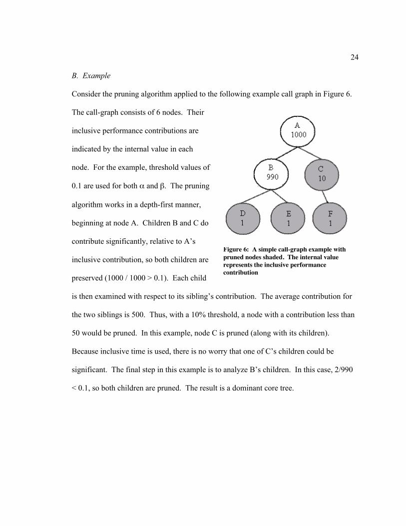
B. Example
Consider the pruning algorithm applied to the following example call graph in Figure 6.
The call-graph consists of 6 nodes. Their
inclusive performance contributions are
indicated by the internal value in each
node. For the example, threshold values of
0.1 are used for both α and β. The pruning
algorithm works in a depth-first manner,
beginning at node A. Children B and C do
contribute significantly, relative to A’s
inclusive contribution, so both children are
preserved (1000 / 1000 > 0.1). Each child
is then examined with respect to its sibling’s contribution. The average contribution for
the two siblings is 500. Thus, with a 10% threshold, a node with a contribution less than
50 would be pruned. In this example, node C is pruned (along with its children).
Because inclusive time is used, there is no worry that one of C’s children could be
significant. The final step in this example is to analyze B’s children. In this case, 2/990
< 0.1, so both children are pruned. The result is a dominant core tree.
Figure 6: A simple call-graph example withpruned nodes shaded. The internal valuerepresents the inclusive performancecontribution
25
C. Selecting an Optimal Core
Once the core components have been identified, an approximately optimal global solution
can be achieved through a brute-force search of the reduced solution space. For this step,
a library was developed that enumerates each realization and evaluates the performance
for each ensemble. Implementations of the same component are grouped into families
(i.e., implementations that may be swapped for one another exist in the same family). In
the example call-graph depicted in Figure 6, each node represents a family member.
Thus, any alternate implementation of component B will exist in the same family as B.
Each family member implements a method that evaluates a hard-coded performance
model. In Figure 7, the example C++ source code is presented for creating a family
member instance of component B (from Figure 6). The getPerfPrediction method accepts
three input values. The first is a vector of values that serve as inputs to the performance
class B : public virtual modeling::AbstractFamilyMember{public:
Figure 7: Example code for implementing a component performance model as a familymember.
26
model. Second, a method name is supplied that indicates which method is being called.
The final input is a map where the result of the performance model evaluation is stored.
After all the family members are declared, a user can explicitly group them into families.
A component ensemble is evaluated by selecting one implementation (i.e., family
member) from each family. The configuration that produces the best result is returned.
27
VI. Validation of the Software Measurement and Optimization Framework
In order to verify the measurement and optimization phases described in the previous
sections, a validation framework was developed. Using “dummy” components that
implement a known performance model enables verification of both the measurement and
optimization stages. These components do not actually perform any work; instead, they
sleep based upon their input parameter(s). Thus, it is trivial to create a test application
that performs to any specification.
In order to test the framework, the component application depicted in Figure 8 was
implemented. Components A
and B each have two
implementations that realize
distinct performance models.
Components C and D are
included as examples of
insignificant components. Thus,
they contribute very little to the
overall performance of the
Figure 8: Simple component application diagram.
28
application. In Figure 9, the wiring diagram for the application is displayed using the
first implementation of components A and B. Similar to the previous figures, uses ports
are situated on the right of a component and provides ports on the left.
Component A’s implementations
execute the performance models y =
2x and y = x2. These models are
graphed in Figure 10. Component
B’s implementations execute the
models y = x3 and y = 2x2. The
models for component B are plotted
in Figure 11. The models for A
and B both have similar Figure 10: The performance models for bothimplementations of component A are plotted.
Figure 9: The component wiring diagram for the validation example.
29
characteristics. Both components
have a clear choice of which
implementation offers better
performance, but this choice
depends upon the input. At input
values x > 2, the ideal
implementation is the realization
executing the lower order
performance model. This attribute
enables the testing of the
implementation selection library
through modification of the inputs.
To test the measurement phase, the components were instrumented using proxies.
Multiple runs using distinct ranges of input values were used in the execution of the
application. The first run consisted of a set of input values of x < 2 to components A and
B; the second run consisted of a set of input values x > 2; the third run consisted of a mix
of input values x >0. Upon completion of the execution of the application, the
performance results were analyzed. The proxies were successful in measuring the
performance of the components, as the measurements matched the expected results. For
each set of input values, the models were evaluated by hand and matched to the results
recorded by the measurement framework.
Figure 11: The performance models for bothimplementations of component B are plotted.
30
In order to test the optimization phase, the application call-graph
in Figure 12 was pruned using the 10% threshold levels. As
expected, the pruner identified components A and B (along with
the Driver) as the core components. Conversely, C and D were
removed from consideration. Using performance models
generated from the measured data, the optimization library was
used to identify the optimal implementations. For the
experiment consisting of input values of x < 2, implementations
A2 and B1 were correctly identified as the optimal choices.
Implementations A1 and B2 were identified as the optimal
choices for the set of input values x > 2. For the third mix, the
majority of inputs were sufficiently greater than two such that A1 and B2 were the clear
choices. The optimization library correctly identified this result.
Figure 12: The call-graph produced bythe componentapplication picturedin Figure 7.
31
VII. Case Study
The performance measurement framework was used to instrument a component-based
scientific simulation. The code simulates the interaction of a shock wave with an
interface between
two gases [26].
The simulation
solves the Euler
equations (a set
of partial
differential
equations) using
structured
adaptive mesh
refinement [27 -
29]. The component application is depicted in Figure 13. In order to simplify the figure,
not all the components needed for execution are included. In the top left is the
ShockDriver that orchestrates the simulation. The AMRMesh component is
responsible for managing the patches of the adaptive mesh refinement strategy. Most of
the inter-processor communication is done within this component. The
StatesConstructor and EFM component are called on a patch-by-patch basis. In
Figure 13: Simplified snapshot of simulation components assembled forexecution.
32
the figure, only two proxies are included due to space constraints, but the simulation was
fully instrumented. There is a GodunovFlux component that is not shown, which can
be substituted for the EFM component. One of the goals of the case study was to compare
the performance between these two components. In addition, the computation time for
the StatesConstructor component and the message passing costs of the AMRMesh
component were analyzed.
The simulation was run on three processors of a cluster of dual 2.8 Ghz Pentium Xeons
with 512 KB caches. The components were compiled using –02 optimization flag for gcc
version 3.2.
In Figure 14, the execution times for the StatesConstructor component across all
three processors are plotted for a single simulation. Note that multiple invocations of the
routine occur with the same array
size. As the size of the input array
increases, the execution times
begin localizing into two groups.
This is the result of the component
using two modes of operation: a
sequential array access mode and a
strided array access mode. For the
smaller, largely cache-resident
Figure 14: Execution time for StatesConstructor.The invoked method has two modes of operation, onethat access the array in a sequential fashion and thesecond accesses the array in a strided fashion.
33
arrays, the two modes perform similarly, but once the cache begins to overflow, the
performance of the strided mode begins to decrease relative to the sequential mode.
Note, that at the largest array sizes, the strided access costs up to four times as much as
the sequential access. The behavior of the Godunov and EFM components is very
similar, because both also utilize the two methods of array access.
The two modes of operation of these
components are invoked in an alternating
fashion during the execution of the
application. As a result, the execution
times of the two modes are averaged to
create a single performance model for
each component. In Figure 15, 16 and 17,
the average execution times for each array Figure 15: Average execution time for StatesConstructor as a function of array size.
Figure 16: Average execution time forGodunov Flux as a function of array size.
Figure 17: Average execution times for EFMFlux as a function of array size.
34
size are plotted. Also included, is the standard deviation. In all three cases, the variation
increases as the array size increases. Regression analysis was used to fit a simple
polynomial or power equation to the mean execution time and standard deviation for each
component. These equations are also plotted in each graph. With the cache-effects
averaged out, the mean execution times scale linearly with the array size.
If TStates, TGodunov and TEFM are the execution times (in microseconds) for the three
components and Q is the input array size, the best-fit expressions plotted in each of the
figures are:
TStates = exp(1.19 log(Q) – 3.68)
TGodunov = -963 + 0.315Q
TEFM = -8.13 + 0.16Q
The corresponding expressions for the standard deviations, σ, are:
σStates = exp(1.29 log Q)
σGodunov = -526 + 0.152Q
σEFM = 66.7 – 0.015Q + 9.24 x 10⁻⁷ – 1.12 x 10⁻¹¹Q3 + 3.85 x 10⁻¹⁷ Q4
These models indicate that the Godunov component offers poorer performance than the
EFM component, especially for large arrays. The variability in timings is also more
severe for the Godunov component. Based on these characteristics, EFM appears to be a
better a choice. However, in reality, scientists often prefer the Godunov solver because
it provides greater accuracy. This is indicative of the necessity to include a quality of
35
service aspect (i.e., accuracy, stability and/or robustness) into the performance model. As
a result, the performance of a component would be relative to the size of the problem as
well as the quality of the solution produced.
In Figure 18 the communication time spent at different levels of the grid hierarchy during
each communication step is
plotted. The primary graph
plots the communication
time for processor 0. The
simulation included a load
balance step, which caused a
new domain decomposition.
This resulted in the
clustering of timings evident
at levels 0 and 2. Ideally,
these clusters should have
collapsed to a single point;
fluctuating network loads
causes the substantial scatter. The inset graph includes the timings across all three
processors. In comparison with the execution times displayed in Figures 15, 16 and 17,
the communication times are similar. This indicates that the application, in its current
context (i.e., problem being solved and accuracy desired), is unlikely to scale well.
Figure 18: Message passing times for different levels of thegrid hierarchy. The clusterings are a result of a re-grid stepthat resulted in a different domain decomposition. INSET:The timings across all three processors.
36
Corroborating this hypothesis is the fact that nearly a quarter of the application’s entire
execution time was spent in message passing.
After analyzing the performance models by hand, the next step was to utilize the
optimization library to select the optimal component applications. In Table 1, the
inclusive and exclusive computation times, along with the inclusive percentage of the
total execution time for each instrumented routine is presented. All values are averaged
over the three processors. The exclusive time is the time spent in a routine minus the
time spent in all instrumented routines called from within the routine. This table clearly
illustrates that not all component contributions are equal. In fact, 10 out of the 15 total
instrumented routines individually contribute less than 10% of the total execution time.
Table 1: The inclusive and exclusive times (in milliseconds) for each of the instrumented routines.The percentage of inclusive time for each routine reltaive to the total execution time is also included.
In Figure 19, the call-graph generated by the measurement framework is presented. As
mentioned in section III, multiple instances of the same component may exist in the call-
graph if a component exists along multiple call-paths (e.g., there are five instances of the
ICC component).
In order to identify the core components, the call-graph is first re-created by the tree
pruning algorithm, which prunes branches based upon the values of the α and β
thresholds. Initially, these thresholds were set to 10%. The resulting call-graph is
depicted in Figure 20, with the pruned branches shaded. The original call-graph
consisting of 19 nodes (12 unique component instances) is reduced to a call-graph of 8
nodes (8 unique component instances). The amount of nodes has been reduced by nearly
60%.
Figure 19: The component call-graph for the shock hydro simulation. Along with the componentname, the inclusive computation time (in microseconds) is included in each node.
38
Figure 20: The call-graph after pruning with 10% thresholds.
Figure 21: The call-graph after pruning with 5% thresholds.
39
The call-graph was also pruned using α and β thresholds of 5% and 20%. The results are
presented in Figures 21 and 22. As would be expected, by lowering both thresholds to
5%, the pruning algorithm removes fewer branches. Also, by increasing the thresholds to
20%, the pruner removes a branch that the 10% thresholds had deemed “significant”.
Thus, manipulating the thresholds may result in a faster (smaller “core” call-graph), yet
less accurate (lower recovery of actual inclusive time of call-graph root from the “core”
call-graph). Although not included in the case study, this flexibility enables a user to
conduct a sensitivity analysis (with respect to α and β), if desired.
Using the core call-graph depicted in Figure 20, the optimal set of implementations is
selected using the library detailed in section III. Using the performance models for each
Figure 22: The call-graph after pruning with 20% thresholds.
40
component that were generated after the performance measurement phase, the library
calculates the optimal configuration of component implementations. For the shock hydro
simulation, the only choice between component implementations was between the EFM
and Godunov components. The library correctly identified the EFM implementation as
the “best” choice, as it resulted in the ensemble with the smallest execution time.
However, as mentioned earlier, Godunov is actually the preferred choice by scientists
due to its quality of service aspects, which are not included in the performance models at
this time.
41
VIII. Future Work
There are numerous opportunities for further investigation in the measurement
framework and optimization library described in this paper. Several of these areas of
interest are listed below.
A. Performance Modeling
The performance models derived in this work are high-level and, as a result, are only
relevant if the component application is executed on a similar cluster of machines. Any
change in the system, such as modifying the cache size, will have a large affect on the
coefficients in models derived in the case study. Ideally, the coefficients should be
parameterized by the processor speed and cache model.
Another performance modeling aspect is how the models are represented in the
implementation selection phase. Currently, the models are hand-coded in and evaluated
by the library. A much more user-friendly and convenient approach would be to have the
library read in the performance models from a file, as an executable expression. One
possible approach would be to express the models using XML [30] or MathML [31] and
have the optimization library parse the file and construct the expressions at runtime.
42
Finally, as mentioned several times, the performance models do not take into
consideration any aspects of quality-of-service. As a result, the optimization library
identified the solver with the shortest time to solution, even though it provides less
accuracy. Future work would allow for these considerations to be included in the
evaluation of the performance models.
B. Dynamic Implementation Selection
One of the interesting features about the Ccaffeine framework is the ability to
dynamically connect components at runtime. This ability allows for the possibility of
swapping a poorly performing component implementation for another on the fly.
Preliminary work on an Optimizer component has begun. This component has the
ability to swap one component instance for another, including inserting a proxy for the
new component and updating all connections to that proxy and to the Mastermind
component. Future work would include enabling the Optimizer to analyze the actual
performance of current components compared to the expected performance. Any
components that are not performing adequately and have an alternate implementation
available, could be swapped.
43
IX. Conclusions
This thesis proposes a software infrastructure designed to non-intrusively measure
performance in a high performance computing environment. Proxies provide a clean and
simple solution to the performance measurement problem. However, in order to model
the performance of a component, the context in which it is used must be taken into
account. Specifically, the input parameters that affect the component’s performance must
be recorded. The proxy is a logical choice to extract this information, but this does not
answer the question of which parameters to extract.
In addition, a technique is described to identify a nearly optimal selection of component
implementations. First, the set of core components is identified by pruning insignificant
branches off of the component call-graph. Multiple implementations of a single
component that exist in the reduced call-graph are grouped into families. A global
performance model is synthesized and evaluated by selecting an instance from each
family and evaluating its individual model and its inter-component interactions. A
complete, nearly optimal solution is achieved by adding in any implementation of the
insignificant components that were pruned in the first step.
In order to test the validity of the measurement and optimization framework, a
verification methodology was also proposed. By implementing “dummy” components
44
that implement a known performance model, the accuracy of the framework may be
evaluated. A test application was presented in which two components each had two
separate implementations. The optimal implementation, for each component, depended
upon the input. Because the dummy components implemented known performance
models, the results of the measurement and optimization phases were easily verified by
hand.
Finally, a case study was presented in which the measurement and optimization
framework was applied to a real life scientific simulation code. The framework enabled
the non-intrusive instrumentation of the application. The measured performance data was
used in the generation of empirical performance models, which were used in the
optimization phase. The case study included a choice of two implementations, and the
optimization phase correctly identified the implementation that provided the smallest
execution time. However, the slower implementation is often the preferred choice by
scientists because it provides better accuracy. This result indicates that a quality of
service aspect (e.g., accuracy, robustness, etc.) is also important in evaluating an optimal
selection.
45
Works Cited
[1] PAPI: Performance Application Programming Interface.http://icl.cs.utk.edu/projects/papi. Accessed May 2005.
[2] PCL – The Performance Counter Library. http://www.fz-juelich.de/zam/PCL.Accessed May 2005.
[3] A. D. Malony and S. Shende, Distributed and Parallel Systems: From Conceptsto Applications. G. Kotsis and P. Kacsuk, Eds. Norwell, MA: Kluwer, 2000, pp.37-46.
[4] D. J. Kerbyson, H. J. Alme, A. Hoisie, F. Petrini, H. J. Wasserman and M. L.Gittings, “Predictive performance and scalability modeling of a large-scaleapplication,” in Proceedings of Supercomputing (SC2001), Denver, CO, 2001.
[5] D. J. Kerbyson, H. J. Wasserman and A. Hoisie, “Exploring advancedarchitectures using performance prediction,” in Innovative Architecture for FutureGeneration High-Performance Processors and Systems, IEEE Computer SocietyPress, 2002, pp 27-37.
[6] The Common Component Architecture Forum. http://www.cca-forum.org.Accessed May 2005.
[7] R. Armstrong, D. Gannon, A. Geist, K. Keahey, S. Kohn, L. McInnes, S. Parkerand B. Smolinski, “Toward a common component architecture for high-performance scientific computing,” in Proc. 8th IEEE Symposium on HighPerformance Distributed Computing (HPDC-8), Redondo Beach, CA, August1999.
[8] CORBA Component model webpage. http://www.omg.com. Accessed July2002.
[9] J. Maloney, Distributed COM Application Development Using Visual C++ 6.0.Prentice Hall, 1999.
[10] R. Englander, Developing Java Beans (Java Series). O’Reilly and Associates,1997.
[11] A. Mos and J. Murphy, “Performance monitoring of Java component-orienteddistributed applications,” in IEEE 9th International Conference on Software,Telecommunications and Computer Networks (SoftCOM2001), Split, Croatia,2001.
46
[12] B. Sridharan, B. Dasarathy and A. Mathur, “On building non-intrusiveperformance instrumentation blocks for CORBA-based distributed systems,” in4th IEEE International Computer Performance and Dependability Symposium,Chicago, IL, March 2000.
[13] B. Sridharan, S. Mundkur and A. Mathur, “Non-intrusive testing, monitoring andcontrol of distributed CORBA objects,” in TOOLS Europe 2000, St. Malo,France, June 2000.
[14] N. Furmento, A. Mayer, S. McGough, S. Newhose, T. Field and J. Darlington,“Optimisation of component-based applications within a Grid environment,” inProceedings of Supercomputing (SC2001), Denver, CO, 2001.
[15] N. Furmento, A. Mayer, S. McGough, S. Newhose, T. Field and J. Darlington,“ICENI: optimization of component applications within a grid environment,”Parallel Computing, 28:1753-1772, 2002.
[16] R. L. Ribler, H. Simitci and D. A. Reed, “The Autopilot performance-directedadaptive control system,” Future Generation Computer Systems, 18:175-187,2001.
[17] R. L. Ribler, J. S. Vetter, H. Simitci and D. A. Reed, “Autopilot: adaptive controlof distributed applications,” in Proceedings of the 7th IEEE InternationalSymposium on High Performance Distributed Computing, Chicago, IL, 1998.
[18] C. Tapus, I-H. Chung and J. K. Hollingsworth, “Active Harmony : towardsautomated performance tuning,” in Proceedings of Supercomputing (SC2002),Baltimore, MD, November 2002.
[19] H. Liu and M. Parashar, “Enabling self-management of component-based high-performance scientific applications,” in Proceedings of the 14th IEEEInternational Symposium on High Performance Distributed Computing (HPDC-14), Research Triangle Park, NC, July 2005.
[20] B. Norris and I. Veljkovic, “Performance monitoring and analysis components inadaptive PDE-based simulations,” submitted to the 24th International Symposiumon Computer Performance, Modeling, Measurements and Evaluation, Juan-les-Pins, France, October 2005. Argonne National Laboratory preprint ANL/MCS-P1221-0105.
[21] TAU: Tuning and Analysis Utilities.http://www.cs.uoregon.edu/research/paracomp/tau. Accessed May 2005.
47
[22] K. Huck, A. Malony, R. Bell, L. Li and A. Morris, “Design and implementationof a parallel performance data management framework,” to be published in Proc.International Conference on Parallel Processing (ICPP-05), Oslo, Norway, June2005.
[23] CCAFFEINE HOME. http://www.cca-forum.org/ccafe. Accessed May 2005.
[24] PDT: Program Database Toolkit.http://www.cs.uoregon.edu/research/paracomp/pdtoolkit. Accessed May 2005.
[25] S. Shende, A. D. Malony, C. Rasmussen and M. Sottile, “A performance interfacefor component-based applications,” in Proc. of International Workshop onPerformance Modeling, Evaluation and Optimization of Parallel and DistributedSystems (IPDPS03), Nice, France, April 2003.
[26] R. Samtaney and J.J. Zabusky, “Circulation deposition on shock-acceleratedplanar and curved density stratified interfaces: Models and scaling laws,” J. FluidMech., 269:45-85, 1994.
[27] M. J. Berger and J. Oliger, “Adaptive mesh refinement for hyperbolic partialdifferential equations,” J. Comp. Phys., 53:484-523, 1984.
[28] M. J. Berger and P. Collela, “Local adaptive mesh refinement for shockhydrodynamics,” J. Comp. Phys., 82:64-84, 1989.
[29] J. J. Quirk, “A parallel adaptive grid algorithm for shock hydrodynamics,”Applied numerical mathematics, 20:427-453, 1996.
[30] Extensible Markup Language (XML). http://www.w3.org/XML. Accessed May2005.
[31] W3C Math Home. http://www.w3.org/Math. Accessed May 2005.