51
UCRL-CR-130725 B334423 Performance of an Island Seismic Station for Recording T-Phases J.A. Hanson H.K. Given

UCRL-CR-130725 B334423
Performance of an Island Seismic Station for Recording T-Phases
J.A. Hanson H.K. Given
DISCLAIMER
This document was prepared as an account of work sponsored by an agency of the United States Government. Neither the United States Government nor the University of California nor any of their employees, makes any warranty, express or implied, or assumes any legal liability or responsibility for the accuracy, completeness, or usefulness of any information, apparatus, product, or process disclosed, or represents that its use would not infringe privately owned rights. Reference herein to any specific commercial product, process, or service by trade name, trademark, manufacturer, or otherwise, does not necessarily constitute or imply its endorsement, recommendation, or favoring by the United States Government or the University of California. The views and opinions of authors expressed herein do not necessarily state or reflect those of the United States Government or the University of California, and shall not be used for advertising or product endorsement purposes.
Work performed under the auspices of the U.S. Department of Energy by Lawrence Livermore National Laboratory under Contract W-7405-ENG-48

Final Report
Performance of an island seismic station for recording T-phases
bY
Jeffrey A. Hanson’ and Holly K. Given2 Cecil H. and Ida M. Green Institute of Geophysics and Planetary Physics
Scripps Institution of Oceanongraphy University of California, San Diego
La Jolla, California 92093
1. NOM* at Center for Monitoring Research, 1300 N. 17th St., Suite 14.50, Arlington, VA 22209 2. Now at the Comprehensive Nulear-Test Ban Treav Organization, Vienna, Austria.
2
Abstract
As part of the International Monitoring System (IMS) a worldwide hydroacoustic
network consisting of 6 hydrophone and 5 island seismic stations has been planned which
will monitor for underwater or low altitude atmospheric explosions. Data from this net-
work is to be integrated with other IMS networks monitoring the Comprehensive Nuclear
Test-Ban Treaty. The seismic (T-phase) stations are significantly less sensitive than hydro-
phones to ocean borne acoustic waves. T-phase signal strength-at seismic stations depends
on the amplitude of the signal in the water column, the hydroacoustic-seismic conversion
efficiency, and loss on the seismic portion of the path through the island. In order to under-
stand how these factors influence the performance of T-phase stations seismic and
hydroacoustic data are examined from instruments currently deployed on or around
Ascension Island in the South Atlantic Ocean.
T-phase recordings for the last 3 years have been collected from the GSN seismic
station ASCN on Ascension Island. Surrounding the island are 5 hydrophones which are
part of the U.S. Air Force Missile Impact Locating System (MILS). Data from this system
have been obtained for some of the events observed at ASCN. Four of the hydrophones
are located within 30 km of the coast while the fifth instrument is 100 km to the south.
Amplitude spectral estimates of the signal-to-noise levels (SNL) are computed and gener-
ally peak between 3 and 8 Hz for both the seismometer and hydrophone data. The seismic
SNL generally decays to 1 between 10 and 15 Hz while the hydrophone SNL is still large
well above 20 Hz. The ratios of the hydrophone-to-seismometer SNL, at their peak in
energy, range between 10 and 100 (20-40 dB) unless a hydrophone is partially blocked by
the Ascension Island landmass. This ratio varies with respect to the azimuth of the arriv-
ing T-phase due to amplitude variations in both the hydrophone and seismic data. Signal
loss at the hydrophones due to island blockage is modeled numerically and then corrected
for. Variations between the corrected hydroacoustic amplitudes and seismic amplitudes are

3
compared with physical parameters such as the gradient of the topography at the island-
ocean interface. T-phases can have various modal structures which will couple into the
island differently. Thus events from the same direction have different signal loss.
1 Introduction
The Comprehensive Nuclear-Test Ban Treaty (CTBT) was signed in 1996 by 141
nations, and although the treaty has not been ratified, it effectively stopped all nuclear test
explosions. A provision in the CTBT calls for an International Monitoring System (IMS)
to monitor treaty compliance. The IMS consists of multiple technologies using global net-
works which will be collected at the International Data Center (IDC) located in Vienna.
The IMS will consist of four networks: seismic, hydroacoustic, infrasonic, and radionu-
elide. The research in this study pertains to the performance of the hydroacoustic network.
The hydroacoustic network will monitor for underwater explosions, although the
scope of the network could expand to include low altitude atmospheric explosions which
may couple into the oceans (Clarke et al., 1997). The network as planned consists of 6
hydrophone stations and 5 T-phase stations which are island seismic stations on mid-ocean
islands. Fig. 4-1 shows the proposed worldwide network. Most of the hydrophones are in
the southern hemisphere where the open oceans allow for long propagation paths and seis-
mic coverage is more sparse. The T-phase stations are generally in the north to extend cov-
erage at a low cost. At the present time, the plan for hydrophones stations is to place two
instruments on either side of an island at a depth approximately corresponding with the
SOFAR channel axis. This requires long lengths of cable to be laid out (> 20 km) which
drives the cost up considerably. Seismic stations which have the recording equipment near
the instruments do not suffer from this additional cost. Because of this, T-phase seismic
stations have been proposed. It is known that island seismic stations do record signals that
travel as acoustic waves through the oceans and convert to elastic waves near the ocean

island interface (Shurbet and Ewing, 1957, Cansi, 1985). It is not known how much signal
loss occurs at this transition and what factors affect the conversion efficiency. The T-phase
station’s effectiveness at recording water borne signals is needed to accurately predict the
performance of the hydroacoustic network as a whole.
4
In this study we examine data collected on and around Ascension Island to deter-
mine potential factors which may influence the T-phase stations performance. The data
sets come from two sources: the IRIS/IDA GSN station ASCN which is on Ascension
Island and hydrophones from the U.S. Air Force Missile Impact Locating System (MILS)
which surround the island. We compare T-phases generated by earthquakes occurring
along the Mid-Atlantic Ridge between the hydrophones and the seismometer to obtain fre-
quency dependent signal loss. We then focus on the relatively stable portion of the spectra
between 3 and 8 Hz to observe factors influencing the signal loss.
2 Instrumentation
Data in this study has been collected from the Global Seismic Network (GSN) sta-
tion ASCN and the MILS hydrophones whose locations are shown in Fig. 4-2. ASCN is a
broadband seismic station which records signals at periods greater than 120 seconds and
frequencies up to 17 Hz. There are two seismometers at ASCN, a borehole instrument and
a surface instrument which are sampled at 20 and 40 Hz respectively (for more detail see
Chapter 2). The IMS proposal calls for the T-phase stations to be sampled at a slightly
higher rate of 50 Hz.
The U.S. Air Force Missile Impact Locating System (MILS) hydrophones were
installed in the 1950’s and 60’s for locating splash downs in the area of missiles launched
from the Kennedy Space Center. Instrument responses were not of great interest because
the splash down creates a sharp delta like function, and it was the time of the arrivals that

5
were of interest. Even if there ever was response information, with the passage of time, it
has been lost. This is unfortunate for our study since we are interested in the frequency
dependent amplitude loss of the T-phase between the hydrophones and seismometer. We
attempt to work around the problem by using signal to noise ratios. Fig. 4-3 shows aver-
age noise spectra for each of the instruments. The main difference between the spectral
levels at the hydrophones begins at 5 Hz and reaches a maximum above 15 Hz (Fig. 4-3).
The largest difference observed is for station U26 which is located 100 km south of the
island. The long cable to this hydrophone is the probable cause of the high-frequency sig-
nal loss, but may also be due to the greater depth at which it is located.
The character of the noise between 2 and 20 Hz at the instrument sites is important
since we are using it to remove the different instrument responses from the signal. The
main assumption is that the “true” noise is the same at each site or at least differs only by a
constant factor. This is a good assumption for most of the hydrophones since they are at
similar depths and distances from Ascension (Fig. 4-4). The noise at the southern hydro-
phone, U26, may differ because the instrument is deeper than the others. McCreery et al.
(1988 and 1993) has found from using hydrophones near Wake Island that the noise levels
between 3 and 6 Hz do not vary much with depth. They do see differences in the 10 to 20
Hz range, but this may be an effect of the hydrophone locations at Wake. Some of the
hydrophones are bottom mounted. Urick (1984) has shown that there is a sudden decrease
in the noise at frequencies greater than -10 Hz below the critical depth (The critical depth
is the depth at which the velocity equals the surface velocity). This is confirmed with
observations in the northeast Pacific Ocean (Morris, 1978, Kibblewhite et al., 1977,
Northrop and Colborn, 1974) and near St. Croix (Urick, 1984). Since the hydrophone U26
is not bottom mounted, but rather 800 meters above the seafloor and above the critical
depth, the noise level should differ by less than a factor of 2. Responses for the instru-
ments around Wake Island (Fig. 4-5) which are similar to the Ascension hydrophones

6
have been retreived.The high frequency response is correlated with cable length (McCre-
ery, et al, 1988) and is sufficient to explain the differences seen in Fig. 4-3 with the excep-
tion of hydrophone U27. This has a significant high frequency loss even though its cable is
unlikely to be longer than U21 or U29. The hydrophone ‘1927 is close to U29 and at nearly
the same depth so that the noise levels are likely the same. The differences in the noise
spectra are probably due to different responses in the hydrophones. These instruments are
old, and it is reasonable to expect that some have degraded over time (McCreery et al.,
1988).
The equivalent noise assumption between the hydrophones and seismometers is
more questionable. To compare ground noise to ocean noise, the ratio of seismic noise to
hydrophone noise spectra are compared with the ratios of the responses between the seis-
mometer and hydrophones. The noise between instruments is not coherent so true transfer
functions cannot be determined. The nominal seismometer response and a “representa-
tive” hydrophone response from the Wake Island instruments is used to calculate the ratio.
The hydrophone response is most representative of hydrophones U29 or U2 1. The ratios
are shown in Fig. 4-6. If the noise is the same at the seismometer and the hydrophones and
the responses are corrected then the predicted ratio (black line) should lie along the noise
ratios. The hydrophone responses from Wake Island go down to only 5 Hz, but they have
been extrapolated to lower frequencies. The resulting ratios are the dashed lines in the fig-
ure. The noise ratio and the response ratio for the surface instrument are similar between
IO and 17 Hz. However, between 6 and 10 Hz there is a small decrease in the noise ratio.
From 4 to 2 Hz there is a large decrease in the noise ratio. The deviation seen in the sur-
face instrument is likely an error in the nominal response. The borehole noise ratios corre-
spond better to the expected response ratios between 2 and 7 Hz. Below 2 Hz there is a
decrease in the noise ratio relative to the response ratio which is likely a difference in the
actual noise levels (Hedlin and Orcutt, 1989, Babcock et al., 1994, Bradley et al., 1997).

7
The seismometer response at ASCN has been called into question by comparing
power spectra of the noise with another GSN station located on St. Helena Island (SHEL)
to the southeast of Ascension. Noise spectra for the borehole and surface instruments at
ASCN and SHEL are shown in Fig. 4-7. The noise for the surface instrument at ASCN is
significantly greater than the borehole above 2 Hz.Estimated transfer functions (ETF)
between the KS-54000 borehole seismometer and the STS-2 are computed using a Welch
periodogram scheme (Cooley et al., 1970) (Fig. 4-8). The nominal predicted transfer func-
tion is also shown. The ETF deviates from the predicted starting near 2 Hz. In contrast, the
estimated transfer function at SHEL is close to the nominal transfer function. In addition
the coherency between signals at the borehole and surface is different at ASCN and SHEL
(Fig. 4-9). The coherency at SHEL remains high out to 8 Hz. The coherency at ASCN, on
the other hand, falls to near zero between 3 and 4 Hz. This indicates a problem with the
ASCN instruments. The borehole instrument is reaching its maximum useful frequency at
5 Hz whereas the nominal response of the STS-2 is flat out to 50 Hz. Thus the borehole
instrument’s response seems more likely to be incorrect, but it is the noise spectrum of the
surface instrument at ASCN that differs from the 3 other seismometers. It appears that
there is an unexpected loss in the STS-2 response at ASCN between 2 and 4 Hz. Since the
borehole noise ratios compare well with the extrapolated response ratios, we conclude that
the ambient noise between 2 and 20 Hz is similar at the hydrophones and the seismome-
ters. Thus using signal-to-noise ratios removes many of the effects of erroneous or
unknown response functions. Although the borehole instrument only records up to 8 Hz,
the results of this study do not change significantly when this seismometer is used instead
of the STS-2.

8
3 Data Analysis
T-phase recordings have been collected from the MILS hydrophones and the seis-
mic station ASCN for 175 earthquakes. The earthquakes most likely occur on the Mid-
Atlantic Ridge from lo to 60” distance from Ascension Island. Fig. 4- 10 shows some
example T-phases. They are generally long in duration (> 100 seconds) and non-impul-
sive. The T-phase has a strong cut-off frequency below 1 and 2 Hz because long period
acoustic waves do not travel far within the sound channel due to interaction with the sea-
floor. Since there is not an impulsive arrival, time windows are picked to encompass the
entire T-phase and are indicated by the solid vertical bars in the figure. Noise windows are
also picked with an attempt to avoid any transient signals including whales.
Power spectra are computed for both the noise and signal windows after applying a
Slepian taper to reduce spectral leakage and maintain frequency resolution (Thompson,
1982). Since instrument responses are unavailable it is necessary to use signal-to-noise
ratios. To avoid a situation where the results depend on the noise at any one instant an
average noise model is used. This is obtained by normalizing all the noise spectra to an
equivalent 100 second window, eliminating unusually high noise spectra, and then averag-
ing the remaining spectra (Fig. 4-3). Likewise the signal spectra are computed using a Sle-
pian taper, but they are not normalized as a stationary signal would be (Priestley, 1981).
The noise is an infinite duration process hence the Fourier transform (FT) increases with
an increasing time window, but the signal is finite in duration and increasing the time win-
dow does not increase the FT (That is assuming that the time-window has included the
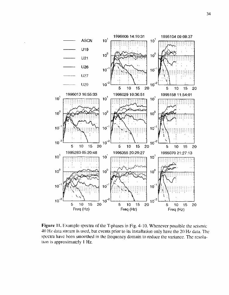
entire T-phase, and that the taper does not significantly affect the signal). Fig. 4-l 1 shows
examples of signal spectra. Here we have used frequency domain averaging to reduce the
variance in the spectra estimates (Priestley, 1981). The choice of time window is a prob-
lem when comparing the signal with noise. Since the length of the time window surround-
ing the T-phase is arbitrary the signal spectrum is not normalized to the window length.

9
The signal-to-noise ratio (SNR) is computed using the noise model for a standard window
length so that ratios may be compared from event to event. The noise model does not nec-
essarily match the actual noise present at the time of the T-phase arrival. In order to deter-
mine when there is actual signal present a noise-to-noise ratio (NNR) is computed by
normalizing the pre-signal noise to a time window equivalent to the signal’s time window
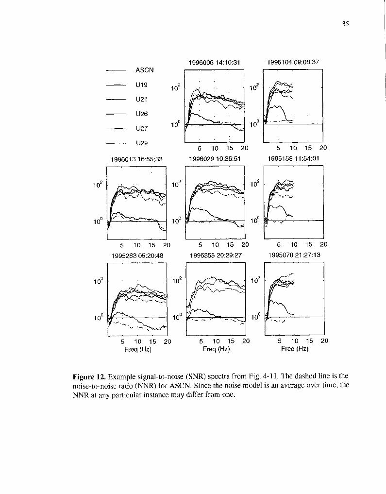
and then dividing by the noise model. Example SNR for the hydrophones and SNR and
NNR for ASCN are shown in Fig. 4-12. The SNR is close to one below 1 Hz. The signal
rises quickly and usually peaks between 3 and 8 Hz. Above that the signal at ASCN
decays away quickly and usually disappears into the noise around 10 Hz. The hydrophone
SNR stays high out past 20 Hz (the nyquist frequency of ASCN). The decrease in SNR for
the seismometer at frequencies above 5 Hz is a real decrease in the signal since the noise is
not increasing at these frequencies (Fig. 4-7). The island is acting as a low-pass filter of
the arriving T-phase diminishing the signal approximately 12 dB/octave relative to the
hydrophones.
The ratio between the SNR at the hydrophones and the SNR at ASCN are taken as
a pseudo-transfer function between the water borne signal and the island seismic signal.
Examples are shown in Fig. 4-13. The function at frequencies with SNR to NNR at ASCN
less than 2 has been blanked out. In general the ratio increases rapidly between 1 and 3 Hz,
flattens out between 3 and 7 Hz, and increases at higher frequencies. Within the 3 to 7 Hz
frequency band the ratio varies widely between events from 3 to 300 a IO to 50 dB loss in
signal at ASCN.
The spectral ratios show great variability among the different events and at differ-
ent frequencies. To reduce the complexity we consider the relatively stable portion of the
spectrum between 3 and 8 Hz. The signal-to-noise ratios over this frequency band are
averaged to obtain one ratio for each T-phase. In addition the events are restricted to a

SNR greater than 20 on at least one hydrophone and a SNR greater than 1 on the seismic
station. In addition to our azimuth estimates from the T-phase arrivals (Chapter 3) these
events had locations, either from the global catalogs or our previous ridge seismicity study
(Chapter 2). The locations provide estimates of distance and azimuth. The subset of events
which met the above criteria consist of 8 1 events which cover a large spread in azimuth.
This is a fairly evenly distributed data set with azimuth. T-phases arrive between -60” to
190” leaving a 1 IO” gap in azimuth to the southwest. -
4 Modeling Transmission Loss
A 2-D parabolic equation method is used to model transmission signal loss
through a range dependent ocean. This is applied to estimate the signal loss at the hydro-
phones due to island blockage and to investigate how the T-phase signal may be affected
due to source and path effects. Parabolic equations have been shown to produce quite
accurate results in ocean acoustics (e.g. Collins et al., 1996). The method solves the for-
ward acoustic wave equation by splitting the problem into a series of range independent
problems and matching boundary conditions between adjacent portions. To derive the par-
abolic equation we follow Tappert (1977) and Jensen et al. (1994). The linear acoustic
wave equation is
q+ldL 0 C2 at2
(1)
where p is pressure and c is the speed of sound in water. The Fourier Transform is taken to
remove the time dependence of the wave equation. In cylindrical coordinates without azi-
muthal dependence the acoustic wave equation is the Helmholtz equation,

where k, = o/cc is the reference wavenumber, and n = ce/c(r,z) is the index of
refraction. We assume a solution of the form,
P(W) = Y (r, z) HA1) (k,r) 9 _ (3)
where HA” is the Hankel function of 0th order and first kind and Y is some envelope
function which varies slowly with range. Substituting this solution into Equation 2 gives,
1 aHy +-Y- r &-
+ Ht1)a2y - + k;n2YH;‘) = 0 O az2
(4)
Grouping the terms with Y, using the property that the Hankel function satisfies the
Bessel equation, and dividing through by Hi” results in,
atu+ 2 ayaHA" -- - 2 H;l)& ar +k;(n2-l)Y = 0. (5)
Next the far field assumption is invoked, k,r D 1 , which allows us to replace the Hankel
function with the asymptotic form,
j’$) (kor) ~ (6)
Substituting this into Equation 5 yields the elliptic wave equation,

a’y . 2
- +2zkos ar2
ay+=+k;(n2-l)Y = 0. az2
This is typically rewritten using the following operators,
a 2 la2 -- P=% Q= n+ 2 2. r----. $)az
The elliptic wave equation then has the form,
[ P2+2ikoP+k%(Q2-l)]Y = 0
12
(7)
(8)
(9)
This can be factored into incoming and outgoing parts with an additional commutator
term,
(P -t= ik, - ik,Q) (P + ik, + ik,Q) Y - iko[P,Q]Y = 0. (10)
The commutator is defined as,
[P,Q]Y = PQY - QPY. (11)
If the propagation medium is range independent then the operators will commute and the
commutator term vanishes. The assumption is made that the range dependence of the
medium is weak enough so that the commutator term may be ignored. In addition the
incoming wave is discarded which leads to,
PY = iko(Q- l)Y. (12)
This is the acoustic wave equation where we have made three approximations: the solu-
tion is in the far-field, the medium varies slowly with range, and there is no significant
back-scattering. We solve for Y in Equation 12 and insert it into Equation 3 to obtain

13
pressure. The Fourier transform takes the solution back into the time domain. To solve
Equation 12 a new operator is introduced,
i a2 4 =n 2-l+-p kiaz2.
(13)
which is related to the previous operator by,
Q = Jrq. (14)
It is the method used to expand this expression into a rational function that gives rise to the
various numerical implementations (Jenkins et al., 1994). If an appropriate reference
speed of sound is picked then q will in general be less than 1. For waves traveling near the
horizontal direction, q will be much less than 1. The more precisely we expand the square-
root in Q the greater the width angle in which our solution will be valid. A simple method
is the binomial expansion where only the first term is kept, Q = 1 + z. This leads to a
rather narrow angle solution, but keeping more terms in the binomial expansion makes
numerical implementation expensive. There are other more accurate ways to expand the
square-root operator into rational functions. The numerical code we use in this study
(RAM, Collins 1993a and 1993b) uses a Pad6 series expansion. The expansion is
where
2 a. = .2 jn h m 2m+ lSln 2m+ 1 ( 1
2 b. .l, m = cos .in:
( 1 2172+1 .
(15)
(16)
(17)

14
Using one term in the above series results in the Claerbout approximation (Claerbout,
1985) which is accurate for propagation angles up to 40”. Adding more terms results in
wider angle approximations.
We use 8 terms in the Pad6 series expansion which results in accurate solutions up
to almost 90” (Collins et al., 1996). The numerical implementation initializes the problem
using a PE self starter (Collins 1993a). The problem is then split into a series of range
independent problems. After propagating the solution through a section, an energy conser-
vation boundary condition is applied to obtain initial conditions for the next range inde-
pendent portion (Collins and Westwood, 1991).
5 Variations in T-phase island transmission
5.1 General
In June of 1995 a series of T-phases arrived at Ascension within 30 minutes of one
another. Variability in the signal loss at the seismometer is observable between the T-
phases shown in Fig. 4-14. The time series for the vertical seismic channel (red) and the
hydrophones (blue) are shown high-pass filtered at 2 Hz. Here we will focus on the two
large events which have epicentral locations in the Preliminary Determination of Epicen-
ters (PDE) and will be referred to as the first and second event. Although both events
occur on the equatorial transform faults of the MAR, they are at different longitudes and
thus arrive at slightly different azimuths. The direction of propagation is indicated by the
colored arrows. The absence of the second event at station U29 (the signal is blocked by
the island) is a clear indication that these events are arriving from different directions. The
hydrophone U19 is well situated to record both events without interference from the island
landmass. The first T-phase appears smaller than the second on the hydroacoustic chan-
nels, but the opposite is true for the seismic channel. Examining the bathymetry around

15
Ascension may provide an explanation of this difference. The average gradient of the edi-
fice radially away from ASCN is steeper for the first event than the second. In general a
steeper gradient will transmit more energy, and thus we would expect the seismic loss to
be less (Jensen and Kuperman, 1980).
5.2 Azimuthal dependence
Determining the signal loss between the water column-and the seismic station
requires that the amplitude of the hydroacoustic signal prior to interaction with the island
be well determined. SNR-to-SNR ratios between hydrophones for each event are exam-
ined to determine the stability of the estimates. Fig. 4-15 shows these ratios as a function
of azimuth. The ratios have been corrected for a 1 /r range dependence from geometrical
spreading and attenuation due to interaction with the seafloor. This correction only affects
the T-phases from nearby events. Even the T-phases that are affected by this correction are
not shifted relative to one another. The exact form of this correction does not significantly
affect our results. The expected transmission loss due to partial island blockage is com-
puted for each of the hydrophones using the parabolic wave equation method described
above. The topography used in the 2-D propagation problem is from a composite map
using many different sources brought together by Minshull et al., 1997. It has a horizontal
resolution on the order of 1 km. The results are the colored lines in Fig. 4-15 plotted to
indicate a loss or gain in the ratios. If the hydrophone SNR in the numerator is partially
blocked the ratio decreases, but if the hydrophone SNR in the denominator is blocked the
ratio increases. These estimates explain much of the variation seen in the ratios. The esti-
mates are robust allowing averaging between instruments to obtain the “true” T-phase sig-
nal strength in the water column prior to interacting with the island.
Ratios are computed between the hydroacoustic and seismic SNR for all the T-
phases. These are shown versus azimuth for each hydrophone (Fig. 4- 16) along with the

16
expected transmission loss (red line) due to partial blockage at the hydrophones. This time
the expected transmission loss only explains a small portion of the variance. Fig. 4-17
shows the histogram of the signal loss for the T-phases after correcting for hydrophone
blockage. The loss varies from 13 to 42 dB with a mean of 26 dB. Plotted in Fig. 4-16 is
the average gradient of the volcanic edifice between 250 and 1750 meters depth radially
out from ASCN (black line). The function has been inverted and scaled to fit on the graph
and is identical for each plot. There is a correlation between the signal ratios and the
changes in slope around the island. The variance increases at azimuths where rapid
changes in the slope occur.
5.3 Distance Dependence
Not all the variation in the T-phase station performance can be explained through
azimuthal variations alone. Fig. 4-18 shows the ratio between two sets of earthquakes
which occur on the Mid-Atlantic Ridge north of Ascension. The seismic signals of the dis-
tant events are 20 dB down relative to the hydrophone signals when compared to the
closer events. The closer group of events occurs on the equatorial transform faults 1100
km to the northeast (Fig. 4-19) and the distant events occur in the north Atlantic more than
5000 km away. The map shows the geodesic paths of the distant events which cross the
equatorial transform fault in between the two closer events. Since the events arrive at
essentially the same azimuth it is difficult to explain the difference as strictly an island
effect. The ratios have been restricted to a very narrow frequency band, so it is not an
effect due to changes in frequency content. The most likely explanation is that the distant
T-phase signals have different spatial structures than the T-phases from the closer earth-
quakes. The two most likely explanations for these differences are different source excita-
tion effects or path dependent effects. Here, both of these factors may play an important
role.

17
6 Discussion
The acoustic T-phase converts into elastic waves near the ocean/island interface.
This is confirmed by comparing the arrival time of the seismic T-phase to the arrival time
of the acoustic wave observed on the hydrophones. Because of the non-impulsive nature
of the T-phase precise measurements are not possible, but it appears the T-phase is travel-
ing near the speed of sound in water. Thus it either converts relatively near the seismome-
ter and/or travels as a very slow elastic (surface) wave. In addition the T-phase energy
traveling along the SOFAR channel will have minimal interaction with the seafloor until
the ocean shoals. Pasyanos and Romanowicz (1997) have observed T-phases traveling
across California at very slow velocities (< 2 km/s) suggesting that the elastic T-phase is a
high frequency surface wave. The seismic T-phase has been modeled as an interface wave
(Stoneley) which then travels as a surface wave on land (Odom, 1997). The amount of
energy that is converted into Stoneley waves at the boundary strongly depends on the
roughness of the seafloor. A smooth interface will only produce a small interface wave
while a rough boundary (100 meter scale length) can have significant energy conversion.
This type of conversion allows for many possible explanations for the variability of the T-
phase station performance.
The conversion strength of the Stoneley waves depends on the interface roughness
(Odom, 1997). We have no direct data on seafloor roughness, but the island sits on a
young (< 6 Ma) volcanic edifice (Nielson and Sibbett, 1996) and does not have significant
sediment cover (van Andel et al., 1973). This would indicate a rough seafloor and an effi-
cient producer of Stoneley waves. The converted phases travel as high frequency surface
waves across the island. The wavelengths are probably less than 400 m which makes the 5
to 10 km they must transverse to the seismometer significant. The Earth’s surface tends to
be strongly heterogenous. This heterogeneity scatters seismic energy which attenuates the
signal in addition to the intrinsic attenuation. We might expect the further the signal trav-

18
els on land the more attenuated it will be. There is some correlation of the conversion effi-
ciency with the distance to shore, but it does not explain the improved conversion seen
between 80” and 110”. Another possibility is different terrains may scatter surface waves
better than others either due to geological or topographic differences. This has been exten-
sively studied by the monitoring community for lower frequency waves (e.g. Shapiro et
al., 1996 and Schweitzer, 1995). There is a marked increase in the signal loss at ASCN for
T-phases arriving from 55” and 80”. At this azimuth, radially away from ASCN, there is a
large undifferentiated trachyte flow consisting in large part of volcanic ash (Nielson and
Sibbett, 1996). This differs from most of the other paths which traverse mafic lava flows.
The azimuth at -6O”, where the variance of the signal loss is large, corresponds to two
large cinder cones near ASCN. If the signal is scattered by the topography the strongest
variability will occur near the cinder cones which in this case is near the seismometer.
This could cause the large variability in the signal loss over relatively small differences in
arrival azimuth.
The variations in the seismic signal for T-phases arriving at the same azimuth but
originating in different regions is most likely due to variations in the energy distribution
with depth. Various factors may influence the spatial structure of the T-phase. The 2-D
parabolic wave equation method described above is used to calculate the transmission loss
(TL) in a range dependent ocean using a point source excitation function. Although a
point source may be an inaccurate description of T-phase generation it is useful in exciting
different modes which propagate down the SOFAR channel. The bathymetry along the
geodesic profile is from Smith and Sandwell’s predicted seafloor topography map (1997).
The ocean environment parameters (temperature and salinity used to calculate sound
speed) have been extracted from the World Ocean Atlas database (Fig. 4-20). We com-
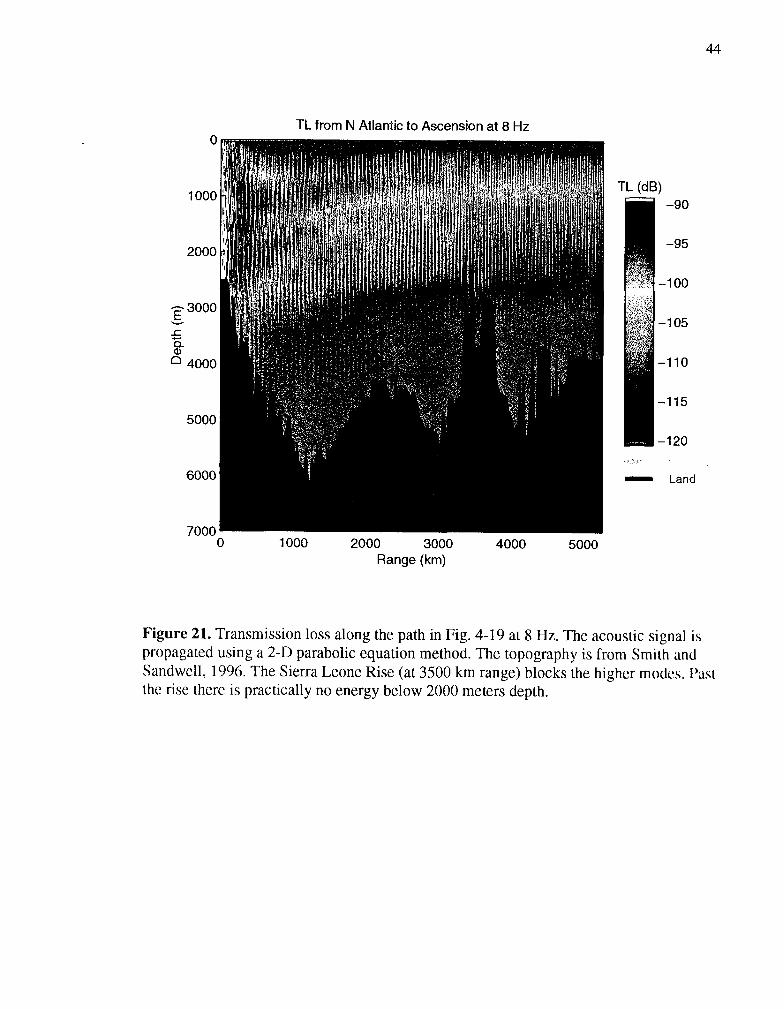
puted TL for three frequencies: 3, 5 and 8 Hz. The resulting TL models are shown in
Fig. 4-21 to Fig. 4-23. The most obvious feature in these figures is the partial blockage of

19
the signal as it crosses the Sierra Leone Rise. The modes at a given frequency have differ-
ent energy distributions with depth (Fig. 4-24). The source can excite different modes
depending on its depth. The energy envelope for mode 1 is a single lobe centered on the
sound channel axis. Mode 2 has two lobes just above and below the axis, and so on. As the
acoustic wave crosses over the seamount the higher order modes are blocked only allow-
ing the low-order modes to pass. Fig. 4-25 shows vertical profiles of the average TL
before and after crossing the Sierra Leone Rise. Prior to the crossing the signal consists of
mode 1 and 2 energy in nearly equal parts, but afterwards the mode 2 energy has been
stripped off. This leaves a much narrower depth range at which there is significant energy.
A similar effect can also be caused by differences in modes excitations. The portion of the
MAP at which distant events occur is shallower than normal. In addition the sound chan-
nel axis is deeper because of the warm, highly saline water entering this portion of the
Atlantic basin through the Strait of Gibraltar (Northrop and Colbom, 1974). Hence the
distant events are more likely to excite the fundamental mode. In either case the energy of
the distant events is concentrated more at the sound channel axis than the energy of the
closer events.
The difference in the seismic signal strength relative to the hydrophones for the
distant earthquakes can be explained by the energy distribution. Each hydrophone samples
the T-phase at only one depth. The seismic signal is generated at the ocean/island interface
and travels along the boundary to the surface. There is energy arriving at the seismometer
from the entire ocean/island interface, and thus the signal power at the seismometer is a
function of the hydroacoustic signal integrated over the entire water column. Since the
distant events have energy concentrated at the sound channel axis, the hydrophones see a
larger signal than the seismometer. From Fig. 4-25 we expect that a hydrophone below the
axis should record a smaller signal. The ratio between a deeper hydrophone and the seis-
mometer will be closer than the more shallow hydrophones. There is some evidence for

20
this in Fig. 4-16 where the ratios for the distant events (in red) are generally smaller and
have a larger variance at station U26 then, for example, U27. This is further evidence that
the seismic T-phase is a more integrated signal than that seen on the hydrophones.
7 Conclusions
T-phases are observed arriving at Ascension Island from various directions at both
hydrophones and seismic stations. Instrument responses are not well known, but signal-to-
noise ratios can be used to eliminate at least some of the response effect. If not all of the
response is removed our results are still practical to the extent that the true noise at the
instrument sites is typical of similar hydrophone and seismic installations. The signal loss
for a given event between the hydrophones and seismometer is fairly constant over the 3
to 8 Hz frequency band. At higher frequencies the island acts as a low-pass filter, and the
seismic signal drops off faster than the hydroacoustic signal by approximately 12 dB/
octave. The T-phase signal generally disappears into the noise between 10 and 15 Hz.
Differences in the signal level between hydrophones for a given T-phase correlate
with island blockage in the 3 to 8 Hz frequency band. The transmission loss at the hydro-
phones from island blockage can be predicted to a large extent using a standard 2-D
hydroacoustic propagation code and seafloor topography with a 1 km resolution. The vari-
ance of signal levels between the hydrophones and the seismic station are greater. The
majority of this variance cannot be explained by hydrophone blockage. The variance in
signal loss has azimuthal dependence and distance dependence. It is not possible to associ-
ate definitively the variance with any one physical property. Possible factors include slope
of the ocean/island interface, roughness of the seafloor, distance from the conversion loca-
tion to receiver, terrain blockage, and spatial structure of arriving T-phase.

21
The apparent signal loss at the seismic station can differ for T-phases arriving from
the same direction but originating at different distances. The T-phase energy distribution
with depth can be expected to differ between the different events. The seismic energy of
the T-phase is a composite of the hydroacoustic T-phase over the entire water column
depth, whereas the hydrophones sample one depth. This indicates that the seismic T-phase
station may potentially estimate the total energy in a T-wave more accurately than a single
hydrophone. This would require detailed calibration of the site.
The dependence of the T-phase amplitude on source excitation or path effects has
important implications for predicting the hydroacoustic network performance. The mini-
mum detectable amplitude at a station is the major factor influencing the effectiveness of
the network. It is not only the size of the source, but also which modes are excited and the
path between source and receiver. In current network prediction models (Farrell and LeP-
age, 1996), a constant dB loss in the SNR is assumed at a T-phase station. This is inade-
quate for ASCN, and is likely wrong for other T-phase stations.
8 Acknowledgments
This study was supported by Intra-University Memorandum Agreement B334398
between University of California, San Diego and Lawrence Livermore National Labora-
tory. David Harris was instrumental in providing support, advice and inspiration through
out the study. Data from the MILS hydrophone network were made available by the Air
Force Technical Applications Center; we thank Frank Pilotte and Ellen Herron for their
assistance in providing this data. The IDA Seismographic Network, an element of the
IRIS Global Seismographic Network, is supported by Incorporated Research Institutions
for Seismology subaward number 0162, the Cecil H. and Ida M. Green Foundation for
Earth Sciences, and Scripps Institution of Oceanography. The seismographic station on
Ascension Island is operated by the staff of the British Broadcasting Corporation.

22
References Babcock, J.M., Kirkendall, B.A. and Orcutt, J.A. (1994) Relationships between ocean bot-
tom noise and the environment. BSSA, 84, 1991-2007.
Bradley, C.R., Stephen, R.A, Dorman, L.M. and Orcutt, J.A. (1997) Very low frequency (0.2-10.0 Hz) seismoacoustic noise below the seafloor, JGR, 102, 11703- 117 18.
Cansi, Y. (1985) T waves with long inland paths; synthetic seismograms, JGR, 90,5459- 5465.
Claerbout, J.F. (1985) Fundamentals of Geophysical Data Processing, Blackwell, Oxford, UK.
Clarke, D.B., Harben, P.E., Rock, D.W. and White, J.W. (1997) Energy coupling of nuclear bursts in and above the ocean surface: source region calculations and experimental validation, Proceedings of the 19th Annual Seismic Research Sympo- sium on Monitoring a Comprehensive Test Ban Treaty, 723-73 1 e
Collins, M.D. and Westwood, E.K. (199 1) A higher-order energy-conserving parabolic equation for range-dependent ocean depth, sound speed, and density. J. Acoust. Sot. Am. 89, 1068-1075.
Collins, M.D. (1993a) A split-step PadC solution for parabolic equation method, J. Acoust. Sot. Am., 93, 1736-1742.
Collins, M.D. (1993b) Generalization of the split-step Pad6 solution, J. Acoust. Sot. Am., 96,382-385.
Collins, M.D., Cederberg, R.J., King, D.B. and Chin-Bing, S.A. (1996) Comparison of algorithms for solving parabolic wave equations, J. Acoust. Sot. Am., 100, 178- 182.
Cooley, J.W., Lewis, P.A. and Welch, P.D (1970) The application of the fast Fourier trans- form algorithm to the estimation of spectra and cross-spectra. J. ofSound and Vibration, 12,339-52.
Farrell, T.R. and LePage, K. (1996) Travel time variability and localization accuracy for global scale monitoring of underwater acoustic events, J. Acoust. Sot. Am., 99, 2572-2574.
Hedlin, M.A.H. and Orcutt, J.A. (1989) A comparative study of island, seafloor, and sub- seafloor ambient noise levels, BSSA, 79, 172-I 79.
Jensen, F.B. and Kuperman, W.A. (1980) Sound propagation in a wedge-shaped ocean with a penetrable bottom, J. Acoust. Sot. Am., 67, 1564-l 566.
Jensen, F.B., Kuperman, W.A., Porter, M.B. and Schmidt, H. (1994) Computational Ocean Acoustics, AIP Press, Woodbury, New York.
Kibblewhite, A.C., Ellis G.E. and Hampton, L.D. (1977) An examination of the deep water ambient noise field in the northeast Pacific Ocean, J. Underwater Acoustics, 27,373.

23
Levitus and Boyer (1994) World Ocean Atlas 1994, NOAA Atlas NESDIS 4, Washington D.C.
McCreery, C.S. and Walker, D.A. (1988) The Wake Island Hydrophone Array, Seis. Res. Lat., 59,22.
McCreery, C.S., Duennebier, F.K. and Sutton, G.H. (1993) Correlation of deep ocean noise (0.4-30 hz) with wind and the Holu Spectrum - A worldwide constant. J. Acoust. Sot. Am. 93,2639-2648.
Morris, G.B. (1978) Depth dependence of ambient noise in the Northeastern Pacific Ocean, J. Acoust. Sot. Am., 64,581-590.
Mu&, W.H. (1974) Sound channel in an exponentially stratified ocean with applications to SOFAR, J. Acoust. Sot. Amer. 66,220-226.
Nielson, D.L. and Sibbett, B.S. (1996) Geology of Ascension Island, South Atlantic Ocean, Geothennics, 25,427-448.
Northrop, J. and Colbom, J. G. (1974) SOFAR channel axial sound speed and depth in the Atlantic Ocean, JGR 79 5633-41.
Odom, R. ( 1997) Personal communication.
Preistley, M.B. (1981) Spectral analysis and time series, Academic Press, New York.
Pasyanos, M.E. and Romanowicz (1997) Observations of T-phases across northern Cali- fornia using the Berkeley Seismic Network, Eos Trans. AGU, Fall Meet. Suppl., 78, F461.
Schweitzer, J. (1995) Blockage of regional seismic waves by the Teisseyre-Tornquist Zone, GJI, 123,260-276.
Shapiro, N., Bethoux, N., Campillo, M. and Paul, A. (1996) Regional seismic phases across the Ligurian Sea; Lg blockage and oceanic propagation, Phys. of the Earth and Plan. Int., 93,257-268.
Shurbet, D.H., Jr. and Ewing, W.M. (1957) T-phases at Bermuda and transformation of elastic waves, BSSA, 47,251-262.
Smith, W.H.F. and Sandwell, D.T. (1997) Global sea floor topography from satellite altim- etry and ship depth soundings, Science, 277, 1956- 1962.
Tappert, ED. (1977) The parabolic approximation method, in Wave Propagation in Under- water Acoustics, Springer-Verlag, New York.
Thomson, D.J. (1982) Spectrum estimation and Harmonic Analysis, IEEE Proc. 70, 1055- 1096.
Urick, R.J. (1984) Ambient Noise in the Sea, Peninsula Publishing, Los Altos California.
van Andel, Tj. H., Rea D. K., Von Herzen, R. P. and Hoskins H. (1973) Ascension Frac- ture Zone, Ascension Island, and the Mid-Atlantic Ridge. Geol. Sot. America Bull. 84, 1527- 1546.

Proposed Hydroacoustic Network
v Hydrophone Stations
A T-phase Stations
Figure 1. Proposed IMS hydroacoustic network. The proposed network consists of 6 hydrophone stations and 5 T-phase stations. The majority of the hydrophones are located in the southern hemisphere while most of the T-phase stations are in the northern hemi- sphere. T-phase stations are seismic island stations used as a cost-saving measure. The hydrophone stations will consist of two instruments on either side of the island in order to reduce island blockage.

40-N
20’N
40”s
60-S
40-w 2O’W 0” 20”E
u19 A A U27
u2, A - u29 ASCN
U26 A I 1 25 km
Figure 2. Locations of instruments and earthquakes used in this study. There are four hydrophones surrounding Ascension Island and one hydrophone 100 km to the south. The hydrophones are part of the U.S. Air Force Missile Impact Locating System (MILS). The seismic station, ASCN, is part of the Global Seismic Network (GSN). The station consists of two seismometers, a Teledyne KS54000 borehole instrument and a Streckeisen STS-2 at the surface. ASCN can record signals up to 17 Hz which is slightly less than the pro- posed T-phase stations which will probably have a maximum frequency of 20 Hz.

- ASCN BOREHOLE
- - - - ASCN STS2
- u19
- u21
- U26
- U27
- u29
26
loo t Average Noise Amplitude Spectra
I I I il ,
1O-B’ I I I 1 o-2 lo-’ 0
Frequc&y (Hz) 10’ IO’
Figure 3. Average noise amplitude spectra. Individual noise spectra are computed from a time window prior to each T-phase, and then spectra with unusually high noise are dis- carded. The remaining spectra are averaged resulting in the noise models for each instru- ment shown above. The seismometer spectra have been scaled to coincide with the hydrophones. Most of the difference in the spectra are due to instrument responses.

27
Instrument Depths and Bathymetry
Sound Channel Axis
Latitude (degrees)
v ASCN
A Hydrophones
Figure 4. Instrument depths. This is a vertical profile from a vantage point east of the island. The open symbol indicates the hydrophone is blocked by the island landmass from this direction. Most of the hydrophones are located near the SOFAR channel axis with the exception of the southern hydrophone which is twice as deep as the others. The seismic station resides on the island at a elevation of 173 meters.

28
Hydrophone Responses from Wake Island -70
I I I I11111 I I I I11111 I I I1111 I I I llllll I I I11111 I I I I11111
I I I I11111 i i i I II
i i iiiii I I IIIII I I lllll
i i’ J/T I I I
L. I I I I IIIU 3 I 1 I i iiiiii
%
t i
-:- &i (iiiii; sNg ; j iii::
---~+;I I I I I .g?-110 - -I-ttt
;
7mM-l-;- I I III t-t l-l
:S I I I IIII I I I III
?iBl!b
I I I II I P I I I11111 I I I I 4 I I I I I III1
I III 17NM I I I I1111 I II II
I
-l--r I I I I11111 I I I iiiiii I I I I11111 I I I I11111 \\
I I III i-i I I I III I
I I i i iiiiii i i i iiiiii I I I11111 I I I I lllll
j \i \ iJb1 ‘i
-1501 . . . . . . I . , ,m,
I I I I11111 I I I I11111 I G l\llLl Ll loo 10’ 10’ lo3
Figure 5. Hydrophone responses from Wake Island. Instrument responses are not avail- able for the Ascension hydrophones, but the figure shows responses for similar instru- ments around Wake Island. The responses are labeled with the corresponding cable lengths in nautical miles. The differences in response are mainly a function of cable length; the longer the cable the more the high frequencies are attenuated.

cul..
u 3
I I1
1111
1 (D
I
I111
111
v)
I I1
1111
1 CH
l+l
I I
I111
111
-J
I I1
1111
1 I
I111
111

0 3 F m -20 s
-60
NOISE SPECTRA ASCN - BOREHOLE & SURFACE
SHEL - BOREHOLE & SURFACE
ASCN & SHEL - BOREHOLE
0 1 2 3 4 5 6 7 6 9 10
Frequency (Hz)
Figure 7. Noise power spectra at ASCN and SHEL for both surface and borehole instru- ments. The spectra have been corrected for instrument response. The borehole instrument at ASCN and the borehole and surface instruments at SHEL all have similar noise spectra. The surface instrument at ASCN deviates around 2 Hz, and at 5 Hz it is almost 15 dB higher than the borcholc instrument. The same effect is seen in spectra of large signals fur- thcr indicating that the difference is not in ground noise.

Transfer function between borehole and surface instruments
__-j ---- j===j===~===f===j===f===~===~=== ---r---,----,---1---1---1---f----~---~---+---
5 ~---r---l----l---7---7---1-*-t--
L ~---t---l----l---~---~---~---~-~ 2 g 10-4 ,---L---I----l__-
s -rrrgz~~l~c~f3z~~ ---- z=z=Fzz=I====I===
l- ----Izzzrl:---l--- 10-5 =---I -=z/=; ==== I___ ------==----~==~~~~~
z===F===I====I=== -------------- I---p---+----+-- ----r---l----I---
1g ~===L====I====l=== --_--------___ =~~~x-Efl=z==I=== z---r---lm---- -----~-==3===3===J===I===f===7---I --- ----~---l----l---~---~---i---i---~---~----
IO-‘- I I I I I I I I I
0 1 2 3 4 5 6 7 8 9 10 Frequency (Hz)
Figure 8. Transfer function estimate between the borehole and surface instruments at ASCN and SHEL. The black line is the predicted transfer function. There is a deviation in The estimated transfer function for ASCN from the predicted transfer function beginning near 2 Hz. The estimate for SHEL agrees with that predicted.

Coherence between surface and borehole instruments
i ; ; ; ;
0.9
0.8
0.7
0.6 i!i 5 tij 0.5
5 0
0.4 ____-_-
0.3
0.2
0.1
0
I I I
.---;---;----;- I I I I I I I I .------- -____ I I I I
1 I
I I
I I I
I 0 1 2 3 4 5 6 7 8 9 10
Frequency (Hz)
Figure 9. Coherence functions between borehole and surface seismometers for ASCN and SHEL. Coherence for the St. Helena instruments is high out to 8 Hz, but at ASCN the coherence drops abruptly at 3 to 4 Hz. This, in addition to Fig. 4-8, indicates a problem with the instrumentation at ASCN.
32

33
1996006 14:09:28 1995104 09:07:13
ASCN SCN ASCN SCN
u19 u19 u21 u21 U26 U26 U27 U27 u29 u29
1996013 16:54:29 1996029 10:35:43 1995158 11:52:29
ASCN SCN SCN ASCN SCN SCN
u19 u19 u19 u21 u21 u21 U26 U26 U26 U27 U27 U27 u29 u29 u29
0 100 0 100 200 0 100 200
1995283 05:19:31 1996355 20:28:09 1995070 21:25:38
ASCN SCN SCN ASCN SCN SCN
u19 u19 u19 u21 u21 u21 U26 U26 U26 U27 U27 U27 u29 u29 u29
0 50 100 0 100 0 100 200 Time (seconds) Time (seconds) Time (seconds)
Figure 10. A series of T-phase recordings for 8 earthquakes. The top trace is the unfiltered seismic data, followed by the 2 Hz high-pass filtered seismic trace, and then the hydro- phone data. The vertical bars indicate the time window used to compute the spectrum.
34
ASCN 10'
u19
u21 IO0
U26 10-l
U27
u29 1o-2
199601316:55:33 ,
10'
IO0
10-l
lo-'
:::::::::;:::::::::: :::: .:::..::::::::. . . . . . . . . . . . . . . . . . . . .
5 10 15 20
1995283 05:20:48 ::::,:::i::::::::::: ::::;:::..:::::::::: . . . .._.............. : :
5 10 15 20 Freq U-4
1996006 14:10:31 ~ 1995104 09:08:37
IO0
10-l
16"
., .
. . .
5 10 15 20 .- 5 10 15 20
1996029 10:36:51 199515811:54:01 10'
IO0
10-l
lo-; _ 5 10 15 20
1996355 20:29:27 1 10'
IO0
10-l
1o-i ,
5 10 15 20 Freq (Hz)
10'
IO0
10-l
1o-2
10'
IO0
10-l
lo-'
5 10 15 20
1995070 21:27:13
j::::::::;: :::;::::::‘.. ::.I::::::::
. . -
5 10 15 20 Freq (Hz)
Figure 11. Example spectra of the T-phases in Fig. 4-10. Whenever possible the seismic 40 Hz data stream is used, but events prior to its installation only have the 20 Hz data. The spectra have been smoothed in the frequency domain to reduce the variance. The resolu- tion is approximately 1 Hz.
1996006 14:10:31 1995104 09:08:37 ~ ASCN
u19 lo2 lo2
u21
U26
U27 loo 10°
U29 5 10 15 20 5 10 15 20
995158 11:54:01
lo2 lo2 lo2
10° 10" 10"
4
5 10 15 20
1995283 05:20:48
5 10 15 20 Freq (Hz)
5 10 15 20
1996355 20:29:27 199507021:27:13 :. . . 4
lo*
-.-_.A .-_ loo '\
I
5 10 15 20 Freq (Hz)
5 10 15 20 Freq (Hz)
Figure 12. Example signal-to-noise (SNR) spectra from Fig. 4-l 1. The dashed line is the noise-to-noise ratio (NNR) for ASCN. Since the noise model is an average over time, the NNR at any particular instance may differ from one.

36
1996006 14:10:31 - ASCN I
u19
u21
U26
U27
U29 I . 1 5 10 15 20
199601316:55:33 1996029 10:36:51
1995104 09:08:37
---I fi I
5 10 15 20
1995158 11:54:01
102. : : - lo2 : ,.: 102 : :
, : * .
I .
7L
t 8
.
loo , I loo loo
5 10 15 20
199528305:20:48 5 10 15 20 5 10 15 20
1996355 20:29:27 199507021:27:13
---1 r--l 10'
loo
10'
loo
5 10 15 20 Freq (Hz)
- I 5 10 15 20 5 10 15 20
Freq U-4 Freq (Hz)
Figure 13. Example hydrophone SNR to seismic SNR spectra from Fig. 4-12. The larger the value, the poorer ASCN recorded the signal relative to the hydrophone. If the true SNR as ASCN is less than 2 the above ratios are blanked out.

ASCN
u21 * * * T
Tr U26 c
U27
Figure 14. Example of conversion variability. Six T-phases arrived at Ascension in June 1995 within 20 minutes of one another. The two large T-phases are from earthquakes located in global catalogs. Both occurred on the equatorial transform faults of the MAR but at different longitudes, and thus they arrive at slightly different azimuths (arrows). The second T-phase appears larger on the hydrophones which are unobstructed by the island, but the opposite is true for the seismic signal. The bathymetry around the island reveals that the gradient radially away from ASCN is steeper for the first event. This provides a possible explanation of the different signal levels at the seismometer.

I A I
lool-++=-! lo-*-
-100 dJ26 / WEDo 200
lo-*- -100 0 100 200
Azimuth (degrees)
Ul9/U26
1O-2L -100 dJ26/U2iiOo 200
I
1O-2L -100 dJ27/U2l3JO 200
1O-2L -100 0 100 200
Azimuth (degrees)
Figure 15. SNR ratios between hydrophones plotted versus azimuth. Average signal-to- noise ratios are measured in the frequency band between 3.5 and 7.5 Hz for each event at each hydrophone. Ratios between hydrophones are taken to examine the consistency of the SNR estimates and are shown versus azimuth. The events have been grouped into dis- tance bins using the color scale in Fig. 4-16. The lines show computed transmission loss due to island blockage. The red and blue lines show expected loss or gain in the ratio depending if the hydrophone SNR is in the numerator or denominator. The calculated transmission loss explains much of the variance in the ratios.

U19 / ASCN
I I
--loo 0 100 200 U26 / ASCN
t I
1O0L -100 0 100 200
U29 / ASCN
I
loo’ ’ I -100 0 100 200
Azimuth (degrees)
U21/ ASCN
U27 / ASCN
1O0L -100 0 100 200
Azimuth (degrees) 0 < 500 km
0 500 - 1500 km
0 1500 - 2500 km
0 2500 - 3500 km
0 > 3500 km
Figure 16. Hydrophone SNR to seismic SNR ratios versus azimuth. This ratio shows the signal loss between the hydrophone and the seismic station between 3.5 and 7.5 Hz. The larger the value the smaller the seismic signal is relative to the hydrophone signal. The ratios are color coded by distance. The expected transmission loss at the hydrophone due to island blockage is shown in red. This calculated loss does not explain much of the vari- ance in the ratios as it did in Fig. 4- 15. The black line is a function of the average slope of the volcanic edifice between 250 and 1750 meters depth. The function is inverted and scaled to fit on the plots in order to see if there is a correlation between gross island topog- raphy and transmission loss.
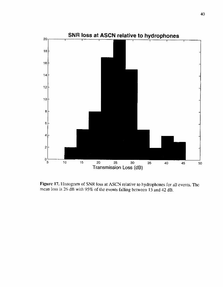
SNR loss at ASCN relative to hydrophones
1U 15 TrL3mis& 35 40 45 50
Figure 17. Histogram of SNR loss at ASCN relative to hydrophones for all events. The mean loss is 26 dB with 95% of the events falling between 13 and 42 dB.

41
Ratio vs Distance at Fixed Azimuth (- -320)
1c
5 10 15 20 25 30 35 40 Distance from U27 (degrees)
45 50
Figure 18. Hydrophone to seismic ratios versus distance. These T-phases arrive from nearly the same azimuth but originate at two different distances. The distant events are poorly recorded at the seismic station relative to the hydrophones. This is most likely due to differences in the T-phase which arrives at Ascension from these two locations. Since the ratios use a narrow band signal it is not a difference in frequency, but more likely a dif- ference in the spatial distribution of the T-phase energy.

30”N
20”N
10”N
30”N
20”N
1O”N
0”
IO?3
20’S 50-w 4O’W 3O’W 2O’W 10-w
Figure 19. Map of T-phase path for events in Fig. 4-18. The T-phases from the distant events originate on the Mid-Atlantic Ridge (MAR), travel pass the Cape Verde Islands, cross over the Sierra Leone Rise and finally cross the MAR again before arriving at Ascension. The closer events straddle either side of the distant path.

Sound of Speed Profile and SOFAR Axis Ill/S
2000 3000 Range (km)
Figure 20. Speed of sound profile along the path shown in Fig. 4-19. The sound channel axis is shown in white. The speed of sound was calculated from the World Ocean Atlas (Levitus and Boyer, 1994) using annual averages. The sound channel is deeper at the northern end because of the warm, saline water from the Mediterranean Sea. The depth of the northern MAR rises to nearly the depth of the sound channel axis.
TL from N Atlantic to Ascension at 8 Hz
1000
2000
E 3ooo 1
%- n 4000
5000
6000
44
TL (dB) , , -90
-95
-100
-105
-110
-115
-120 ..s
- Land
2000 3000 Range (km)
Figure 21. Transmission loss along the path in Fig. 4-19 at 8 Hz. The acoustic signal is propagated using a 2-D parabolic equation method. The topography is from Smith and Sandwell, 1996. The Sierra Leone Rise (at 3500 km range) blocks the higher modes. 1’3~1 rhe rise there is practically no energy below 2000 meters depth.

45
1000
2000
E 3ooo II
% I2 4000
5000
6000
7000 2000 3000
Range (km) 4000 5000
TL from N Atlantic to Ascension at 5 Hz
TL (dB) -90
-95
-100
-105
-110
-115
-120 I i : , i , L : ,
- Land
Figure 22. Transmission loss along the path in Fig. 4-19 at 5 Hz. See caption for Fig. 4- 21.

46
1000
2000
E 3ooo AZ P I2 4000
5000
6000
7000
TL from N Atlantic to Ascension at 3 Hz
-95
-100
-105
-110
-115
Land
2000 3000 Range (km)
4000 5000
Figure 23. Transmission loss along the path in Fig. 4-19 at 3 Hz. See caption for Fig. 4- 21.

47
Energy Distribution of First 4 Normal Modes at 8 Hz
Figure 24. Normal modes within the SOFAR channel. The first 4 modes at 8 Hz using the canonical velocity profile (Munk, 1974) are shown to demonstrate the variability of energy distribution with depth.

Signal Loss Before and After Crossing Sierra Leone Rise
50
100
250
300 125 120 115 110 105 100
Transmission Loss (dB)
Figure 25. Vertical TL profile before and after the Sierra Leone Rise from Fig. 4-22. The signal consists of mode 1 and 2 energy prior to crossing the rise, but there is only signih- cant energy in mode 1 after passing over the seamount. Most of the hydrophones are at 800 meters depth which is near the maximum of mode 1. The southern most hydrophone is deeper at about 1600 meters (Fig. 4-4).

Technical Inform
ation Departm
ent • Lawrence Liverm
ore National Laboratory
University of C
alifornia • Livermore, C
alifornia 94551

![Seismic collapse performance of special moment steel …earthquake.hanyang.ac.kr/journal/2017/[2017]Han et al-Seismic... · Seismic collapse performance of special moment steel frames](https://static.documents.pub/doc/80x56/5b8364d47f8b9adc698cfc15/seismic-collapse-performance-of-special-moment-steel-2017han-et-al-seismic.jpg)
![SEISMIC PERFORMANCE AND ECONOMIC …SEISMIC PERFORMANCE AND ECONOMIC FEASIBILITY ... ... 4]](https://static.documents.pub/doc/80x56/5e730ef63a752763c8260684/seismic-performance-and-economic-seismic-performance-and-economic-feasibility-.jpg)


