Performance of Institutional Trading Desks: An Analysis of Persistence in Trading Cost

Amber Anand Syracuse University amanand@syr.edu

Paul Irvine

University of Georgia pirvine@uga.edu

Andy Puckett

University of Missouri puckettw@missouri.edu

Kumar Venkataraman

Southern Methodist University kumar@mail.cox.smu.edu

This draft: March 2009

Abstract

Using a unique dataset of institutional investors’ equity transactions, we document that institutional trading desks can sustain relative performance over adjacent periods. The best institutional desks exhibit a persistent pattern of negative trading cost, suggesting that skilled traders have the ability to create positive (investment) alpha through their trading strategies. We investigate several possible explanations for the institutional trading cost persistence including broker selection, trading style and commissions. We identify a set of trading decisions that are associated with performance. Our study contributes to the relatively unstudied literature on the performance of institutional trading desks. Our findings suggest that trading cost is a source of mutual fund performance persistence and that broker selection based on past performance is an important dimension of the money manager’s Best Execution obligation. *We thank Hank Bessembinder, Jeffrey Busse, Paul Goldman, Jeff Harris, Swami Kalpathy, Qin Lei, Eli Levine, Stewart Mayhew, Tim McCormick, Rex Thompson, Ram Venkataraman, Andres Vinelli, Kelsey Wei and seminar participants at the Commodity Futures Trading Commission (CFTC), Financial Industry Regulatory Authority (FINRA), Indian School of Business, Nanyang Technological University, National University of Singapore, Securities and Exchange Commission (SEC), the 3rd Annual IIROC conference, Singapore Management University and Southern Methodist University for comments. We are grateful to ANcerno Ltd. (formerly the Abel/Noser Corporation) and Judy Maiorca for providing the institutional trading data. Venkataraman thanks the Marilyn and Leo Corrigan Endowment at Southern Methodist University for research support. Anand gratefully acknowledges a summer research grant from the office of the VP of Research at Syracuse University. Corresponding author: Kumar Venkataraman, kumar@mail.cox.smu.edu.

Performance of Institutional Trading Desks: An Analysis of Persistence in Trading Cost

Abstract Using a unique dataset of institutional investors’ equity transactions, we document that institutional

trading desks can sustain relative performance over adjacent periods. The best institutional desks exhibit a

persistent pattern of negative trading cost, suggesting that skilled traders have the ability to create positive

(investment) alpha through their trading strategies. We investigate several possible explanations for the

institutional trading cost persistence including broker selection, trading style and commissions. We

identify a set of trading decisions that are associated with performance. Our study contributes to the

relatively unstudied literature on the performance of institutional trading desks. Our findings suggest that

trading cost is a source of mutual fund performance persistence and that broker selection based on past

performance is an important dimension of the money manager’s Best Execution obligation.

1

1. Introduction

Trading costs for institutional investors are economically large.1 In the context of illiquid stocks,

Keim (1999) shows that, over the period 1982-1995, a passive small-cap fund that pays attention not only

to tracking error but also to trading cost can earn an annual premium of 2.2% over a pure indexing

strategy. This is one example of how trading costs can significantly impact portfolio performance. We

illustrate the importance of trading cost to institutional performance by documenting the magnitude of

heterogeneity in trading cost, and more importantly, the persistence in trading cost across institutional

investors. Our findings suggest that trading cost is a source of mutual fund performance persistence and

that the positive risk-adjusted performance observed for some funds can be partly attributed to the skills

of the institutional trading desk.

To understand the contribution of the trading desks to institutional performance, we examine

institutional investor equity transactions compiled by ANcerno Ltd. (formerly the Abel/Noser

Corporation). The data contain approximately 35 million order tickets that are initiated by 664

institutional investors and facilitated by 1,137 brokerage firms over a seven-year period, 1999-2005,

representing $22.9 trillion in trading volume. The database is distinctive in that it contains a complete

history of each order ticket, each typically resulting in more than one execution, sent by an institutional

investor to a broker. This history includes stock identifiers that help obtain relevant data from other

sources, and more importantly for this study, codes that identify the institution and the broker associated

with each ticket.

Our study contributes to the literature on the performance of financial intermediaries. Prior

academic research has focused on the performance of money managers, such as mutual funds, hedge

funds and institutional plan sponsors. However, there is little academic work examining the performance

of another category of financial intermediaries, namely trading desks, responsible for trillions of dollars in

1 For example, using institutional data provided by the Plexus Group, Chiyachantana, Jain, Jiang and Wood (2004) reports average trading costs of 41 basis points for 1997-98 and 31 basis points for 2001. Other related studies include Chan and Lakonishok (1995), Keim and Madhavan (1997), Jones and Lipson (2001), Conrad, Johnson and Wahal (2001) and Goldstein, Irvine, Kandel and Wiener (2008).

2

executions each year. Since Jensen (1968), many of the tests in the performance measurement literature

examine performance persistence: whether past performance is informative about future performance. In

the context of mutual funds, recent studies that focus on public information and managerial skill

(Kacperczyk and Seru (2007)), short measurement periods (Bollen and Busse (2005)) or use a Bayesian

framework (Busse and Irvine (2006)), find strong evidence that funds sustain relative performance

beyond expenses or momentum over adjacent periods. This evidence on consistent performance by funds

raises the important question regarding the source of persistence. Most prior work attributes some part of

persistence to fund manager skill. However, Baks (2006) decomposes outperformance into manager and

fund categories and reports that manager skill accounts for less than half of fund outperformance and that

the fund is more important than the manager. If managerial stock picking prowess is the primary driver

then why would the fund be a source of relative performance?

Besides research and stock picking abilities, the institution’s quality of trade execution, guided by

its rules governing best execution, can be an important component of portfolio performance.2 Portfolio

managers rely on the buy-side trading desks to obtain the best implementation of their investment ideas.

A trading desk can add value to an institution’s portfolio by supplying expertise in execution analysis. It

is therefore natural to ask whether the execution process can be a source of persistence in institutional

performance. The detailed transaction level ANcerno dataset seems particularly well suited for studying

whether institutional trading desks can sustain relative performance over adjacent periods and contribute

to fund performance persistence.

Our paper focuses on a literature that examines heterogeneity in transaction cost for specific

groups of intermediaries. Linnainmaa (2007) uses Finnish data to argue for differences in execution costs

across retail and institutional broker types. Conrad, Wahal and Johnson (2001) document the relation

between soft-dollar arrangements and institutional trading cost. Keim and Madhavan (1997) and

Christoffersen, Keim and Musto (2006) show dispersion in trading costs of institutions and mutual funds.

2 A popular definition of best execution is “the best price available in any market at the time of the trade” (see Wagner and Edwards (1993), Macey and O’Hara (1997)). The authors note that given the multiple dimensions of execution quality and the complexity in measuring execution cost, this definition of best execution is too simplistic.

3

Yet, institutional execution is a joint production process that incorporates the decisions of both

institutions and their brokers. Our paper complements this work by using more extensive set of domestic

trading data that allow us to integrate both institutional execution and broker execution into a single

framework. We extend the literature on trading cost by testing for persistent trading skill. To our

knowledge, this is the first study to examine performance persistence of buy-side institutional desks and

sell-side brokers from the perspective of execution quality. Our analysis provides insights on the linkage

between fund performance and trading cost and also has implications for the Best Execution obligation of

institutional trading desks.

We find that institutional trading desks can sustain relative performance over adjacent periods.

Our measure of trading cost, the execution shortfall, compares the execution price with a benchmark price

when the institutional trading desk sent the ticket to the broker. It reflects the bid-ask spread, the market

impact, and the drift in price while executing the order but excludes brokerage commissions. We sort

institutional trading desks based on execution shortfall during the portfolio formation month and create

quintile portfolios. We find that institutional trading desks with the lowest (highest) execution shortfall in

the portfolio formation month continue to exhibit the lowest (highest) execution shortfall during the next

four months. In each of these months, the difference in execution quality across the best and worst

performing institutional quintiles is approximately 62 basis points. The results are similar when we

control for the economic determinants of trading cost, such as ticket attributes, stock characteristics and

market conditions, in a regression framework. Remarkably, the best institutional trading desks exhibit a

persistent pattern of negative execution shortfall, suggesting that the trading desk of the best institutions

can help create positive (investment) alpha through their trading strategies.

We investigate several possible explanations for the institutional trading desk performance

persistence. An important decision made by the trading desk is broker selection. We therefore examine

whether some brokers can deliver better execution consistently over time. We find that brokers ranked as

top performers during portfolio formation month continue to exhibit the lowest execution shortfall in

subsequent months. The difference in performance across the top and bottom broker quintiles is

4

approximately 28 basis points. These findings suggest that the brokers exhibit significant heterogeneity in

execution quality and that the top brokers can sustain their advantage over adjacent periods. We note that

the best brokers in our sample can execute trades with no price impact. The latter finding is particularly

striking since our dataset contains the trades initiated by large investors.

We next examine whether the persistence in institutional and broker performance is independent,

or whether one effect subsumes the other effect. We find that there exist significant differences in

execution cost across institutional desks that are unique to the institution and not systematically related to

the broker. Further, the combined effects of the institution and the broker are economically large. For

example, the difference in execution cost between the [top institution, top broker] and the [bottom

institution, bottom broker] exceeds 100 basis points, suggesting that mutual fund performance persistence

can be partly attributed to trading cost.3

We fail to find support for the hypothesis that trading cost persistence is driven by institutional

trading style such as trading in stocks with high ex ante information asymmetry, which could widen bid-

ask spreads. Yet, we can identify a set of trading decisions that are associated with performance. The

worst performing institutional trading desks specify low commission (or ‘touch’) execution venues,

suggesting they tend to focus on the explicit trading cost. However, this choice is sub-optimal and can

ultimately cost the institution considerably more in price impact than the savings in commissions. Our

evidence also suggests that the simple strategies such as splitting orders or concentrating order flow with

fewer brokers help institutions receive better execution.

To aid institutions in broker selection, we report on characteristics that are associated with broker

performance. The best brokers tend to be boutique firms rather than generalists, and specialize by sectors

or industries. On average, these brokers charge higher commissions and more often work the ticket to

obtain better prices. The worst brokers in our sample do not appear to be predominantly soft dollar

3 Recent studies estimate that the spread in fund performance between top and bottom quintile is around 3 percent to 6 percent per year (see Busse and Irvine (2006), Kacperczyk et al. (2006)). Assuming an average annual mutual fund turnover rate of 100 percent (see Edelen et al. (2007)), trading costs can help explain a significant portion of the persistence in fund performance.

5

brokers. We also document that the institution’s choice of the broker is sensitive to past performance. The

top (bottom) brokers for an institution receive more (less) order flow and have a higher (lower) likelihood

of being among the institution’s top 10 brokers (based on volume) in future periods. Our evidence

suggests that the worst performing brokers slowly lose their market share.

This study is also of interest to money managers, institutional trading desks, regulators and

investors. Best execution has been the subject of recent regulatory attention under U.S. Regulation

National Market System (Reg NMS) and European Union’s Markets in Financial Instruments Directive

(MiFID). In defining Best Execution, regulators in the U.S. have emphasized the fiduciary duty of brokers

and fund managers to obtain the best value for the investment decision.4 Our results suggest that broker

selection based on past trading performance is an important dimension of the money manager’s fiduciary

obligation. However, because brokers provide a package of non-execution related services to institutions

(such as prime brokerage services, IPO allocations, and research) and we have no way of measuring these

potentially offsetting benefits, it is very difficult in reality to measure Best Execution. While our findings

suggest that some institutions consistently obtain poor executions and can benefit from better rules for

broker selection, we cannot necessarily conclude that these decisions violate their fiduciary obligation.

For brokerage firms, our finding that institutional order flow is sensitive to past execution quality

suggests that institutions are paying close attention to the value of the brokerage services. For institutional

trading desks, the ability of skilled traders to create positive (investment) alpha, and to sustain superior

performance over adjacent periods, emphasize their contributions to investment performance. From a

regulatory perspective, the study should inform regulatory initiatives such as SEC Concept Release S7-

12-03, which considers “whether mutual funds should be required to quantify and disclose to investors

the amount of transactions costs they incur, include transaction costs in their expense ratios and fee tables,

or provide additional quantitative or narrative disclosure about their transaction costs.” Our evidence

suggests that increased disclosure on mutual funds’ trading costs can provide useful incremental

4 FINRA 2320(a) states “The Best Execution Rule require a member, in any transaction for or with a customer, to use reasonable diligence to ascertain the best inter-dealer market for a security and to buy or sell in such a market so that the resultant price to the customer is as favorable as possible under prevailing market conditions.”

6

information for investors’ decision making process.

This paper is organized as follows. In Section 2, we describe the institutional trading process and

review the literature on measuring trading cost of mutual funds. Execution cost measures and the sample

selection are presented in Section 3. In Section 4, we report the results on performance of institutional

trading desks. In Sections 5 and 6, we consider possible explanations for performance persistence. Section

7 summarizes the findings and concludes.

2. Background

2.1. The Institutional Trading Process

A typical order originates from the desk of a portfolio manager at a buy-side institution. Portfolio

managers hand off the order with some instructions on order urgency (trading horizon) to the buy-side

trading desk. The trading desk makes a set of choices to meet the best execution obligation, including

which trading venues to use, whether to split the order over the trading horizon, which broker(s) to select

and how much to allocate to each broker. The allocation to the broker, defined in our analysis as a ticket,

may in turn result in several distinct trades, or executions, as the broker works the order.

The trading desk can add value to an institution’s portfolio by supplying expertise in execution

analysis, offering advanced technological systems, and selecting a strategy that best suits the fund

manager’s motive for trading. For example, a portfolio manager who wishes to raise cash by doing a

program trade, or a value manager trading on longer-term information, can be better served with passive

trading strategies, such as limit orders (see Keim and Madhavan (1995)). In contrast, portfolio managers

who trade on short lived information, or index fund managers who try to replicate a benchmark index may

be better served with aggressive trading strategies, such as market orders, to assure quick execution.5 The

5 However, the evidence on the linkage between trader identity and order urgency is relatively weak. Keim and Madhavan (1995) find that the institutional investors in their sample trade primarily using market orders and “show a surprisingly strong demand for immediacy, even in those institutions whose trades are based on relatively long-lived information. Consequently, it is rare that an order is not entirely filled”. Similarly, Chiyachantana et al. (2004) report that the average fill rate for their sample of institutional orders exceeds 95% for all sample years. The ANcerno dataset does not provide information on the fill rates for a ticket. We rely on prior literature and assume that the fill rate for a ticket is 100%.

7

trading problem is especially difficult for orders that are large relative to daily security trading volume.

For such orders, the displayed market liquidity is insufficient and it becomes important to signal trading

interest in order to draw out reactive traders (Harris (1997)). However, exposing the order would allow

traders to front run the order and increase the price impact. Large traders may choose to use the services

of an upstairs broker or purchase liquidity from a dealer at a premium (see Madhavan and Cheng (1997)).

More influential institutions could insist that their broker provide capital to facilitate their trades. In an

increasingly fragmented marketplace, a trader’s skill lies in detecting pools of hidden liquidity and

responding quickly to order imbalances to improve execution performance (see Bessembinder, Panayides

and Venkataraman (2009)).

2.2. Measuring Execution Costs of Mutual Fund Trades

Prior research has recognized that trading cost can be a drag on managed portfolio performance

(see, for example, Carhart (1997)). Since transaction data for mutual funds are not publicly available, the

previous literature relating mutual fund performance and trading cost has relied predominantly on

quarterly ownership data. A commonly used measure for trading cost is the mutual fund turnover, defined

as the minimum of security purchases and sales over the quarter, scaled by average assets. Turnover is a

noisy proxy for trading cost as it assumes that funds trade similar stocks and incur the same level of

trading costs in executing their trades.

Another measure, proposed by Grinblatt and Titman (1989) and implemented recently by

Kacperczyk, Sialm and Zheng (2006), is based on the return gap between the reported quarterly fund

return and the return on a hypothetical portfolio that invests in the previously disclosed fund holdings. As

noted by Kacperczyk et al. (2006), the return gap is affected by a number of unobservable fund actions

including security lending, timing of interim trades, IPO allocations, agency costs such as window

dressing activities, trading costs and commissions, and investor externalities. While the return gap can

gauge the aggregate impact of the unobservable actions on mutual fund performance, the authors note that

it is impossible to clearly attribute its effect to any specific action.

Some studies, such as Wermers (2000), have estimated the execution cost of mutual funds using

8

the regression coefficients from Keim and Madhavan (1997), who examine trading cost for a sample of

institutions between 1991 and 1993. Edelen, Evans and Kadlec (2007) propose a new measure that

combines changes in quarterly ownership data on a stock-by-stock basis with trading costs estimated for

each stock from NYSE TAQ data.6 However, as acknowledged by these studies, the stock-specific per-

unit trading cost obtained from NYSE TAQ data or estimated using Keim and Madhavan coefficients

would significantly understate the heterogeneity in execution cost across mutual funds. This is because

trading cost can vary significantly across institutions, even controlling for stock characteristics or

investment style, reflecting differences in the skills across trading desks (see Keim and Madhavan

(1997)).7

The distinguishing feature of our study is that we can estimate with greater precision the total

trading cost, including price impact and commissions, associated with each institution. By analyzing

actual institutional trade-by-trade data, we are able to capture the heterogeneity in trading efficiency or

skills across trading desks. Further, since the dataset contains the complete trading history for each

institution, we can observe the entire fund trading activity, including purchases and sales of the stock

made within a quarter, which cannot be observed from changes in quarterly snapshots of fund holdings.

Moreover, the focus of our investigation differs considerably from related work in the literature.

We examine separately the role played by institutional-execution versus broker-execution in a single

framework and discover persistent patterns in institutional trading cost, suggesting that the execution

process can serve as an explanation for mutual fund performance persistence.

3. Execution Shortfall Measure and Descriptive Statistics of the Sample

3.1. Execution Shortfall Measure

Our measure of trading cost, the execution shortfall, compares the execution price of a ticket with

the stock price when the trading desk sends the ticket to the broker. The choice of a pre-trade benchmark

6 The TAQ data do not identify the broker or the institution associated with a transaction. Nor does it allow the researcher to identity multiple transactions associated with the originating ticket. 7 Consistent with previous studies, we observe in our sample that institutions exhibit significant difference in trading cost for stocks with similar characteristics.

9

price follows prior literature (see, for example, Keim and Madhavan (1997), Chan and Lakonishok

(1995)) and relies on the implementation shortfall approach described in Perold (1988).8 We define

execution shortfall for a ticket as follows:

Execution Shortfall(b,t) = [(P1(b,t) – P0(b,t)) / P0(b,t)] * D(b,t) (1)

where P1(b,t) measures the value weighted execution price in ticket ‘t’ with multiple executions, P0(b,t) is

the price at the time when the broker ‘b’ receives the ticket, and D(b,t) is a variable that equals 1 for a buy

ticket and equals -1 for a sell ticket.

3.2. Sample Descriptive Statistics

We obtain data on institutional trades for the period from January 1, 1999 to December 31, 2005

from Ancerno Ltd. (formerly the Abel/Noser Corporation). ANcerno is a widely recognized consulting

firm that works with institutional investors to monitor their equity trading cost. ANcerno clients include

pension plan sponsors such as CALPERS, the Commonwealth of Virginia, and the YMCA retirement

fund, as well as money managers such as MFS (Massachusetts Financial Services), Putman Investments,

Lazard Asset Management, and Fidelity. Previous academic studies that have used ANcerno data include

Goldstein, Irvine, Kandel and Wiener (2008), Chemmanur, He and Hu (2009), and Lipson and Puckett

(2007).

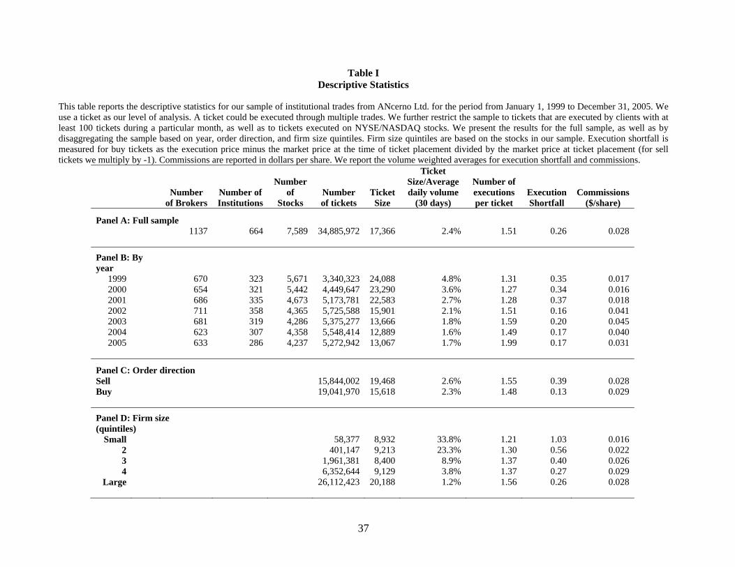
Summary statistics for ANcerno trade data are presented in Table 1. The sample contains a total

of 664 institutions, responsible for approximately 34 million tickets and leading to 87 million trade

executions. For each execution, the database provides the identity of the institution, the broker involved

in the trade, the CUSIP and ticker for the stock, the stock price at placement time, date of execution,

execution price, number of shares executed, whether the execution is a buy or sell, and the commissions

paid. The institution’s identity is restricted to protect the privacy of ANcerno clients; however, each

8 Some studies (see Berkowitz, Logue and Noser (1988), Hu (2005)) have argued that the execution price should be compared with the volume-weighted average price (VWAP), a popular benchmark among practitioners. Madhavan (2002) and Sofianos (2005) present a detailed discussion of VWAP strategies and the limitations of the VWAP benchmark. Among them, the VWAP can be influenced by the transaction that is being evaluated. Further, an execution may outperform the VWAP but in fact may be a poor execution because the broker has delayed the trade and the stock price has drifted away since the time when the broker received the ticket.

10

institution is provided with a unique client code to facilitate identification.9 Conversations with ANcerno

confirm that the database captures the complete history of all transactions of the portfolio managers.10

Over the sample period, ANcerno institutional clients traded more than 755 billion shares, representing

more than $22.9 trillion worth of stock trades. The institutions are responsible for 7.97% of total CRSP

daily dollar volume during the 1999 to 2005 sample period.11 Thus, while our data represents the trading

activities of a subset of pension funds and money managers, it represents a significant fraction of total

institutional trading volume.

We use stock and market data from the CRSP and TAQ databases to complement our analysis of

the ANcerno trade data. We obtain the market capitalization, stock and market returns, daily volume and

listing exchange from CRSP, and daily dollar order imbalance from TAQ. For a stock, the dollar order

imbalance is defined as the daily buyer-initiated minus seller-initiated dollar volume of transactions

scaled by the total dollar volume. TAQ trades are signed as buyer or seller-initiated using the Lee and

Ready (1993) algorithm.

There are several notable time-series patterns in institutional trading observed in Table I, Panel B.

The number of brokers and institutions in the database remains relatively constant. The number of stocks

has declined, from 5,671 in 1999 to 4,237 in 2005, while volume has been steady, particularly since 2000

at over 5 million tickets. The average ticket size has declined from 24,088 in 1999 to 13,067 in 2005, with

a significant decline in 2002 coinciding with decimalization. In the recent sample period, the ticket is

broken up more frequently, as evidenced by the increase in number of executions per ticket. The

execution shortfall has declined, particularly since 2001, while the commissions increased markedly in

9 In addition, the database provides summary execution information for each ticket, including the share-weighted execution price and the total shares executed. ANcerno provides two separate reference files – one for broker and the other for client type - that we merge with the original trade data. 10 ANcerno receives trading data directly from the Order Delivery System (ODS) of all money manager clients. The method of data delivery for pension plan sponsors is more heterogeneous. Our main findings are similar when we examine money managers and pension plan sponsors separately. 11 We calculate the ratio of ANcerno trading volume to CRSP trading volume during each day of the sample period. We include only stocks with sharecode equal to 10 or 11 in our calculation. In addition, we divide all ANcerno trading volume by two, since each individual ANcerno client constitutes only one side of a trade. We believe this estimate represents a lower bound on the size of the ANcerno database.

11

2001 before declining in 2005. Sofianos (2001) remarks that the reduction in spreads that accompanied

decimalization in 2001 made the NASDAQ zero commission business model untenable, and institutions

began paying commissions on NASDAQ trades. This change is coincident with the increase in

commission costs that we observe.

To minimize observations with errors, we impose the following screens: (1) Delete tickets with

execution shortfall greater than an absolute value of 10 percent, (2) Delete tickets with ticket volume

greater than the stock’s CRSP volume on the execution date,12 (3) Include common stocks listed on

NYSE and NASDAQ, (4) Delete institutions with less than 100 tickets in a month for the institution

analysis and delete brokers with less than 100 tickets in a month for the broker analysis, and (5) Delete all

observations where the commission per share for a ticket is $0.10 or greater.

From Panel C of Table I, we note that the execution shortfall for sell tickets (39 basis points)

exceeds those for buy tickets (13 basis points), consistent with Chiyachantana et al. (2004). This partly

reflects the fact that the average sell order is larger than the average buy order. In Panel D, we report

summary statistics based on CRSP market capitalization quintiles formed in the month prior to the trading

month examined. Although the average ticket size for Small quintile firms is only 8,932 shares, the

average ticket represents a remarkable 33.8 percent of the stocks’ daily trading volume. The average

ticket size in Large quintile firms exceeds 20,000 shares but represents only 1.2 percent of the stocks’

daily volume. Clearly, tickets in Small quintile firms are more difficult to execute, experiencing an

average execution shortfall of 105 basis points. In contrast, the execution shortfall for Large quintile firms

is only 26 basis points.

4. Performance of institutional trading desks

4.1 Preliminary examination of persistence in institutional trading cost

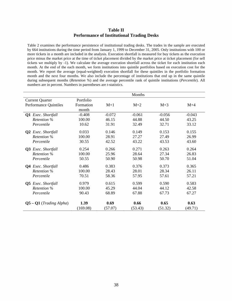
Table II presents our initial examination of performance of institutional trading desks. For each

12 While this filter eliminates only 0.04% of all observations, we recognize that some tickets may correspond to executions in non-US markets. We have replicated the analysis without this filter and obtained similar results.

12

institution, we calculate the execution shortfall for a ticket and then the volume weighted execution

shortfall across all tickets for the month. We place institutions in quintile portfolios (1-best, 5-worst)

based on monthly execution shortfall during the formation month (month M). Table II presents the time

series average of equally weighted portfolio performance of institutions in month M.13

Not surprisingly, given the idiosyncratic nature of trading performance, there is a large and

significant difference of 139 basis points between the best and worst institutions in the portfolio formation

month. The best performing institutions execute trades with a negative execution cost of 41 basis points,

while the worst performing institutions execute trades with an execution cost of 98 basis points. However,

every random distribution has dispersion and there are a myriad of market conditions that can affect the

execution quality of particular trades. Thus, our test of trading desk performance merely uses the portfolio

formation month as a benchmark for sorting trading desks into performance quintiles.

The key test of trading desk performance examines whether a quintile’s relative performance

persists into the future. In Table II, we report the average execution shortfall in future months M+1

through M+4 for institutions sorted into execution cost quintiles in month M. In month M+1, we note that

institutions placed in (best performing) quintile 1 during month M report a negative execution cost of 7

basis points. In contrast, institutions placed in (worst performing) quintile 5 achieve an average execution

cost of 62 basis points. We also note that the execution shortfall in month M+1 increases monotonically

from quintile 1 to quintile 5. The difference in month M+1 performance between quintile 1 and quintile 5

is 69 basis points (t-statistic of difference = 57.07). In further support of performance persistence, we find

that trends discussed above continue to be observed in month M+2 through M+4, with the average Q1-Q5

difference in execution cost being 66, 65 and 63 basis points respectively (all statistically significant).

Importantly, the difference in execution cost of approximately 65 basis points is also economically large.

As additional tests of performance persistence, we examine two statistics, the retention

percentage (Retention %) and the percentile rank (Percentile). The Retention % for quintile 1 is the

percentage of institutions ranked during month M in quintile 1 that continue to remain in quintile 1 when 13 Value weighted construction produces similar results.

13

ranked on execution shortfall in a future month. Retention % helps examine whether both good and poor

performance is more persistent than performance in the middle quintiles. As a benchmark, we expect the

Retention % to be 20 percent for any quintile in a future month if performance rankings based on month

M have no predictive power. However, from Table II, the Retention % in the extreme quintiles are as high

as 46 percent, suggesting that the ranking based on month M is informative about future performance.

The second measure, Percentile rank for quintile 1, reports the average percentile rank based on

the execution shortfall estimated in future months for institutions ranked in quintile 1 during month M. By

construction, the Percentile for quintile 1 (quintile 5) in month M is 10 (90). Under the null hypothesis

that month M rankings have no predictive power, we would expect the Percentile for any institution

quintile in future months to be 50. Alternatively, if the month M rankings have predictive power, we

expect the Percentile for the best institutions in future months to be less than 50 (above average) and

Percentile for the worst institutions to be greater than 50 (below average). We observe that, consistent

with the alternative hypothesis of performance persistence, the Percentile for the best and the worst

performing institutions exhibit significant deviations from 50 in the predicted direction.

4.2. Multivariate analysis of persistence in institutional trading cost

While the prior section finds evidence of institutional performance persistence, we don’t know

why. It is possible that some institutions initiate easier to execute tickets than other institutions as a result

of their distinct investment models. Therefore, it is important to control for ticket attributes, such as ticket

size and direction, as well as stock characteristics, such as market capitalization, stock price and trading

volume. Further, institutional trading can be influenced by market conditions, such as stock volatility and

short-term price trends (Griffin, Harris and Topaloglu (2003)), and by the market on which the stock

trades (Huang and Stoll (1996)). Thus, cost comparisons across institutions or over time must control for

the difficulty of trade.

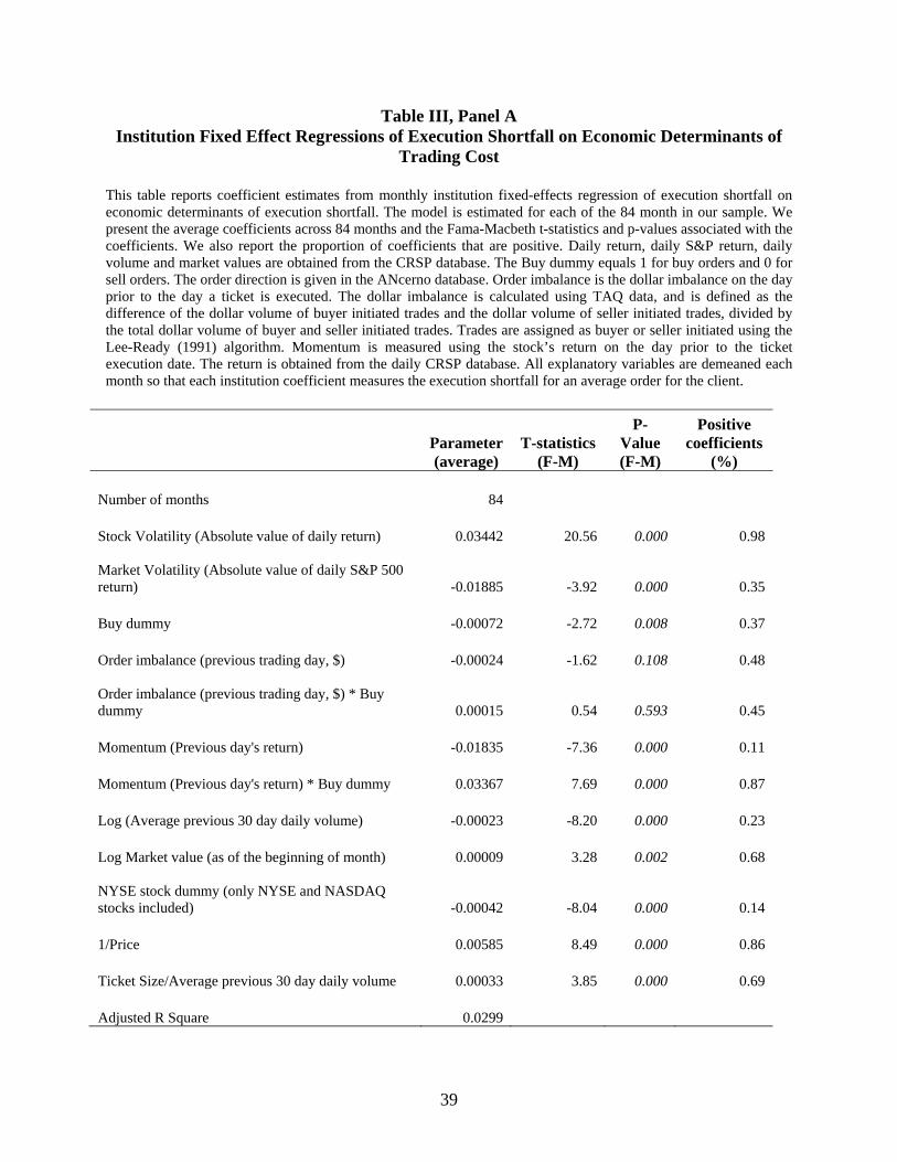
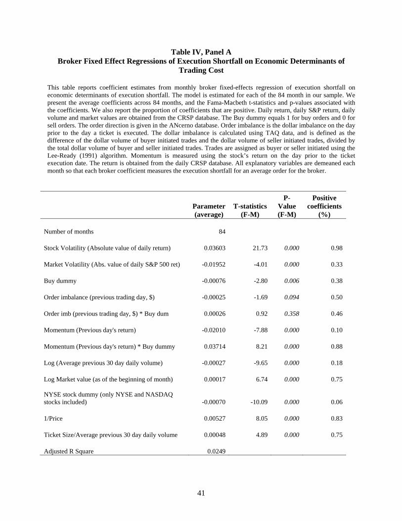
We estimate monthly, institution fixed-effect, regressions of execution shortfall on the economic

determinants of trading cost. These variables include stock and market return volatility on the trading day;

14

a Buy indicator variable that equals one if the ticket is a buy order and equals zero otherwise; the

imbalance between buy and sell orders based on the prior trading day; a variable that interacts order

imbalance and the buy indicator; stock momentum, measured as the prior day’s return; a variable that

interacts momentum with the buy indicator; the stock’s average daily volume over prior 30 trading days;

stock market capitalization at the beginning of the month; and the inverse of stock price. As a measure of

trade difficulty, we include ticket size normalized by the stock’s average daily trading volume over prior

30 days. The regression coefficients allow us to estimate the ticket’s expected execution cost based on

trade difficulty, which serves as the benchmark for the performance measurement of trading desks.14,15

Our objective is to evaluate the performance of trading desks, holding ticket, firm and market

variables at common, economically relevant levels. Following Bessembinder and Kaufman (1997), we

therefore normalize every individual explanatory variable by deducting the sample mean of the

explanatory variable for the month. Note that only the intercepts are affected by the normalization. In this

specification, each institution fixed-effect coefficient can be interpreted as the average execution cost for

the institution in the month, evaluated at the monthly average of ticket, firm and market characteristics.

We term the institution coefficients as institution trading alphas, since the cross-sectional variation in

institution coefficients can be attributed at least in part to the skill of the institutional trading desk.

In Table III, Panel A, we report the average coefficient across 84 monthly regressions, the Fama-

Macbeth t-statistics and p-values based on the time-series standard deviation of estimated coefficients,

and the percentage of monthly regression coefficients with a positive sign. The estimated coefficients for

the control variables are of the expected sign and statistically significant; the exception being order

imbalance variables that are not significant at the five percent level. For example, execution shortfall

increases with stock volatility, reflecting the higher cost of a delayed trade in volatile markets, but

14 To explore the possibility of a non-linear relation between the ticket size and execution shortfall, we estimate an alternative model using the log of normalized ticket size (instead of the normalized ticket size). The results are similar to those reported in the paper. 15 We replicate the analysis using an execution shortfall measure that controls for the overall market movement on ticket’s execution day, and find similar results. Specifically, following Keim and Madhavan (1995), we use an adjusted execution shortfall measure, which deducts the daily return on the S&P 500 index. The adjusted measure is appropriate if some trading desks hedge their exposure to market movements using a futures contract or an ETF.

15

declines with the stock’s trading volume.16 Trading against the previous day’s momentum reduces

execution cost, while trading with the momentum trend increases execution cost. Seller-initiated tickets

are more expensive to complete than buyer-initiated tickets, reflecting the bearish market conditions

during much of the sample period. Consistent with prior work, NYSE-listed stocks are less expensive to

complete than NASDAQ stocks. Finally, execution shortfall costs increase with ticket size, suggesting

that larger orders are more expensive to complete.

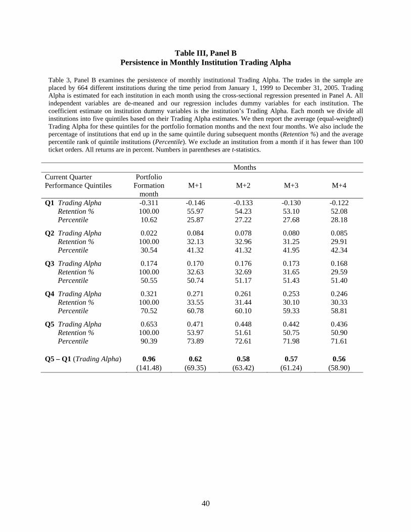
In Panel B of Table III, we report on tests of persistence in trading alpha. The tests use the

approach outlined for the unadjusted data in Table II. The most striking difference between the two tables

is the reduction in the spread during the portfolio formation month between quintile 1 and quintile 5. This

difference, which was 139 basis points in Table II, is reduced to 96 basis points in the regression

framework. Despite the reduction in spread across quintile portfolios, our conclusions on the performance

of institutional trading desks are unchanged. In future month M+1, the difference in institutional

performance between quintile 1 and quintile 5 is 62 basis points (t-statistic of difference = 69), which is

similar to the 69 basis points reported in Table II. Persistence is also of similar magnitude for future

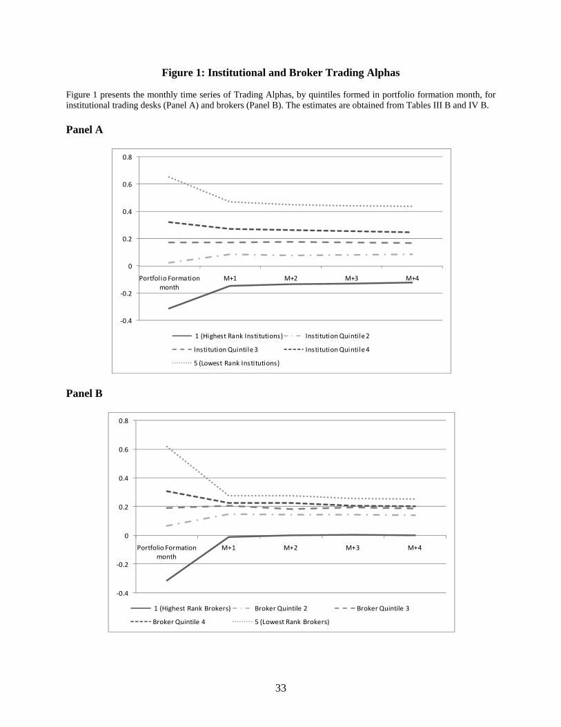
months M+2 through M+4 (see Figure 1, Panel A), suggesting that the main conclusions from Table II

are robust to controlling for differences across institutions in ticket attributes, stock characteristics and

market conditions.

Even more striking is the finding that the coefficients on quintile 1 institutions are robustly

negative in future months M+1 through M+4, averaging between -12 and -15 basis points. A persistent

pattern of negative execution shortfall suggests that the trading desks of the best institutions can help

create positive (investment) alpha through their trading strategies. Recall that the mutual fund literature

identifies a small subset of funds that exhibit persistent patterns in positive risk adjusted returns. Our

findings imply that the trading desk can contribute to positive abnormal performance of the institutional

investors. Institutional desks can obtain negative trading costs by providing liquidity; i.e., by posting limit

16 The positive coefficient in trading cost regressions on market capitalization with control for trading volume is a common finding in empirical microstructure research (see, Stoll, 2000, for example). Prior research has attributed this to the high correlation between trading volume and market capitalization.

16

orders or responding to order imbalances.

Our other measures of trading desk persistence are generally stronger in the regression framework

than those reported in the univariate framework. The retention ratios show that best performing

institutions in the portfolio formation month have close to a 56 percent chance of being in the best

performing quintile in month M+1, and comparable percentages in the other future months. The worst

performing institutions also exhibit persistence by this measure with over 50 percent of the quintile 5

institutions remaining in the bottom performing quintile in future months. The best performing

institutions in the portfolio formation month have significantly higher percentile performance ranks in

future months. Quintile 1 institutions have average percentile ranks (out of all institutions) of between

25.9 and 28.2. In contrast, the bottom performing institutions have percentile ranks considerably lower in

the future months varying between 71.6 and 73.9. Overall, the results in Table III strongly suggest that

past trading desk performance is informative about future trading desk performance.

5. Possible explanations of persistence

5.1. Evidence from brokers

We investigate several possible explanations for persistence in institutional trading alpha. An

important decision made by the trading desk is broker selection. Brokers themselves may possess above

average or below average ability to execute trades. We therefore examine whether some brokers can

deliver better execution consistently over time. We repeat the regression analysis in Table III, Panel A

with broker fixed effects rather than institution fixed effects. Following prior notation, we term the broker

fixed effect as the broker’s trading alpha. The control regression coefficients are presented in Table IV,

Panel A and as before in Table III, Panel A, the only insignificant coefficients are associated with the

order imbalance variables. All other coefficients are of similar significance and sign.

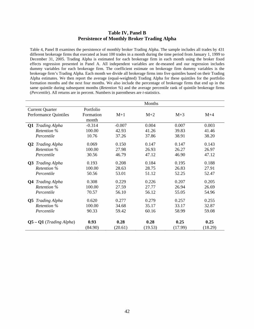
Using the broker alpha estimates from Table IV, Panel A, we construct broker quintiles in

portfolio formation month M by ranking the brokers each month by their trading alpha. The average

trading alpha for a broker quintile over the sample period is presented in the portfolio formation month

17

column of Table IV, Panel B. In the portfolio formation month, the spread between the top and bottom

quintiles in the sample is 93 basis points.

More importantly, a significant part of this difference in execution cost is persistent (see Figure 1,

Panel B). In future month M+1 the difference between the best and worst performing brokers, at 28 basis

points, is economically and statistically significant. The difference in broker performance persists in

future months M+2 through M+4, averaging between 28 and 25 basis points. Further, we find that the

execution shortfall for best brokers (quintile 1) is insignificantly different from zero for future months

M+1 through M+4. The result that the best brokers in our sample can execute tickets with no price impact

is particularly striking since we examine tickets initiated by large institutions. The result likely reflects the

skill of the brokerage firms in working the order and detecting pools of hidden liquidity.

Other tests also support the hypothesis that broker performance is persistent. Forty-two percent of

the brokers placed in quintile 1 during month M are also ranked independently in the same quintile in

future month M+4. Similarly, almost 33 percent of brokers ranked as the worst performers in month M

continue to be ranked as the worst performers in month M+4. We find that the Percentile for the best

brokers in future months is in the high-30s and the Percentile for worst brokers is in high 50s. These

findings provide additional support that past broker performance is informative about future broker

performance. 17

5.2. The joint performance of institutional desks and brokers

The results thus far indicate that both institutional trading desks and brokers exhibit persistence in

relative performance. The difference between the best-performance and the worst-performance institution

or broker quintiles is economically large enough to have a considerable influence on measures of

portfolio performance. The ultimate source of these performance differences cannot be discerned by the

results reported thus far as they have only demonstrated that execution cost persistence exists and that it is

17 The spread between the top and bottom performers is also significant in future months M+5 to M+12. Specifically, in month M+12, the spread for institutional desks is 47 basis points (t-statistic=42.13) and for brokers is 20 basis points (t-statistic=13.75). Detailed results are available from the authors.

18

both statistically and economically significant. If certain brokers are skilled at execution, then perhaps

institutional clients of these brokers will tend to exhibit performance persistence. Conversely if certain

institutions are better traders, perhaps it is the case that institutions are skilled and they just tend to

concentrate their trading with particular brokers.18 Alternatively, it is possible that both specific brokers

and certain institutions have superior (or inferior) execution performance.

5.2.1. Analysis of Trading Volume Market Share

We examine the order routing decisions to see whether the best institutions trade predominantly

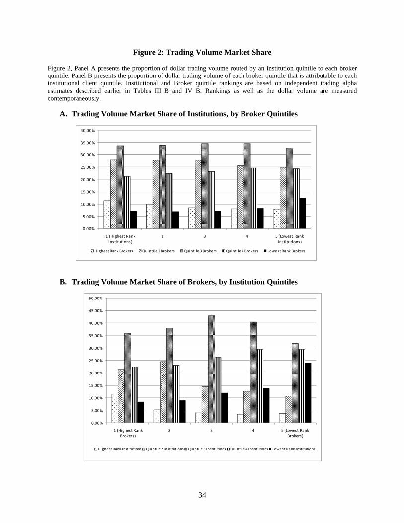
with the best brokers, and vice-versa. In Figure 2, Panel A, we plot the proportion of dollar trading

volume routed by an institution quintile to each broker quintile, in Month M. Institution and broker

quintile rankings are based on independent trading alpha estimates described earlier in Tables III B and

IV B. Brokers ranked as average (quintile 3) are the largest brokers in that they execute about 33 percent

of the institutional volume. There is little variation in their market share across institution quintiles. The

best performing institutions execute 39 percent of volume with above-average brokers (the top two

quintiles) and 28 percent of volume with below-average brokers (the bottom two quintiles). In contrast,

the worst performing institutions execute 33 percent of volume with above-average brokers and 37

percent of volume with below-average brokers. While broker selection can serve as a partial explanation

for patterns in institutional performance, there is no evidence of significant clustering of institutions with

certain broker types.

Similarly, broker performance may be a function of the quality of their institutional clientele.

Figure 2, Panel B presents the proportion of dollar trading volume for each broker quintile that is

attributable to each institutional quintile. Institutions ranked as average (quintile 3) are the largest in that

they account for about 31% to 40% of the order flow across all broker quintiles. The best performing

brokers receive 33% of their order flow from above-average institutions (the top two quintiles) and 30%

of the order flow from below-average institutions (the bottom two quintiles). In contrast, bottom

18 Goldstein et al. (2008) report that institutions tend to concentrate the order flow with a few brokers. This concentration causes significant differences in the client lists of brokers and the broker lists of clients.

19

performing brokers receive only 14.5% of their order flow from above-average institutions and 53.5% of

their order flow from below-average institutions. If certain institutions trade badly, then the brokers

receiving order flow from these institutions will perform poorly. Clearly, the significant clustering

observed in Figure 2, panel B suggests that broker performance can be assessed only after controlling for

institution performance.

5.2.2. Evaluating independent patterns in institution and broker persistence

Trading performance is a joint production problem as it takes both a broker and an institutional

desk to execute a ticket. We attempt to isolate the performance of each contributor to the execution by

first, for each portfolio formation month, calculating institution trading alphas and sorting them into

quintiles. For each month, we also (independently) calculate broker trading alphas and sort them into

quintiles. We then use the institution and broker quintile designations to assign each ticket to one of 25

quintile intersection (5×5) portfolios. With dummy variables representing each of the 25 portfolios, we

estimate the trading alpha for each of the 25 portfolios in the portfolio formation month and in months

M+1 through M+4 separately. As before, the estimation in months M+1 through M+4 uses portfolios

formed on the basis of broker and institution rankings in month M, and the same control variables as those

in Tables III, A and IV, A.

We use our 25 formation-month portfolios to address the joint production problem in two

complementary ways. First, in Table V, Panel A, note that each broker quintile is associated with five

performance-ranked institution portfolios. To assess evidence on institutional persistence after controlling

for broker effects, we examine institutional persistence within each broker quintile. That is, for each

broker quintile, we construct the difference between the trading alphas of the portfolio of worst-

performing institutions and the portfolio of the best-performing institutions. For each broker quintile, the

difference in institutional performance is reported during portfolio formation month M and future months

M+1 through M+4. This test can illustrate whether results such as the average 62 basis point performance

difference across institutional quintiles in month M+1 from Table IV, Panel B is systematically related to

20

the choice of the broker.

The general conclusion from Table V, Panel A is that institutional execution quality differences

are not systematically related to broker execution quality. Although the largest performance differential

between the best and worst institutional quintiles is observed among the best performing brokers (72 basis

points in month M+1), note that institutional performance differentials do not monotonically deteriorate

with broker quality. The second largest institutional performance difference occurs in broker quintile 5,

the worst performing brokers.

Conversely, it may be true that certain institutions possess execution skills and when these

particular institutions concentrate their trading with certain brokers, as observed in Figure 2 Panel B, they

produce the patterns in broker performance as observed in Table III. So, can broker persistence be driven

by institution-specific characteristics, such as trading style? To examine this hypothesis, we reverse the

analysis in Panel A. For each institutional quintile, we calculate the performance differential between the

best and worst performing brokers in portfolio formation month and future months. Analysis of these

results allows us to determine whether broker performance differences are systematically related to

institutional style.

The results in Panel B indicate that broker performance differences are again the largest for

tickets received from the best performing institutions, ranging from 31 to 35 basis points in future months

M+1 to M+4. Similar to Panel A, the second largest broker differences are observed in orders received

from the worst performing institutions. Yet again, we cannot support the theory that broker performance

differences are due solely to institutional effects, such as trading style. Across institutional quintiles, we

observe persistent difference in broker performance of at least 20 basis points across all future months.19

We therefore conclude that past broker performance is informative about future performance after

19 As a robustness check, we examine broker persistence in an institution fixed effects specification where a institution specific indicator variable, which equals one for an institution’s ticket and equals zero otherwise, is included in the regression. This specification controls for the difference in investment style across institutions by examining the performance of brokers within an institution. We find that the difference between the best and the worst brokers is 21 basis point (t-statistics=16.33) in month M+1 and 18 basis points (t-statistic=14.06) in month M+4.

21

accounting for differences in institutional clientele. An important implication is that institution should

select brokers based on past performance. We provide some empirical evidence consistent with this

behavior in Section 6.4.

Figure 3 presents a graphical representation of the execution shortfall across the broker-institution

portfolios in month M+1. Several observations are noteworthy. Within broker quintiles, there exist

significant differences in trading cost across institutional trading desks that are unique to the institutions.

Similarly, within institutional quintiles, we observe a monotonic improvement in performance from the

worst to the best performing brokers in future month M+1. From this evidence, we conclude that both

specific institutions and brokers have superior (or inferior) execution performance and this performance is

predictable based on past performance. Importantly, the combined effects of the institution and broker are

economically large. For example, the difference in execution cost between the [top institution, top broker]

and the [bottom institution, bottom broker] exceeds 100 basis points.

5.3. Can trading style explain institutional persistence?

Although certain institutions consistently obtain poor executions, the institutions may not violate

their fiduciary Best Execution obligations if their approach reflects a trading style that realizes the

maximum value of the firm’s investment ideas. For example, a fund manager who trades on short-term

momentum or a short-lived information advantage may choose aggressive strategies that incur high

execution cost but enhance portfolio alpha. The 5×5 portfolio approach detailed above controls for the

effect of the institution’s style on broker persistence but not on trading desk persistence. So, how much of

trading desk persistence is driven by the institutional style?

A limitation of the ANcerno data is that the institutions’ identity is not revealed. To proxy for the

trading style, we examine price patterns observed subsequent to a ticket’s execution (post-trade price

drift), defined as:

Post Trade Price drift (b,t) = [(Pclose(t) – P1(b,t)) / P1(b,t)] * D(b,t), (2)

where Pclose(t) is the stock’s closing price on the day after the day of ticket execution. If the institution’s

22

investment style necessitates urgency in executing the ticket (e.g., based on short lived information), we

hypothesize that the post-trade price movement will be observed in the direction of the institution’s ticket

(i.e., upward drift for a buy ticket and downward drift for a sell ticket). Thus, if persistence is explained

by trading style, the worst performing institutions should exhibit the largest post trade price drift.

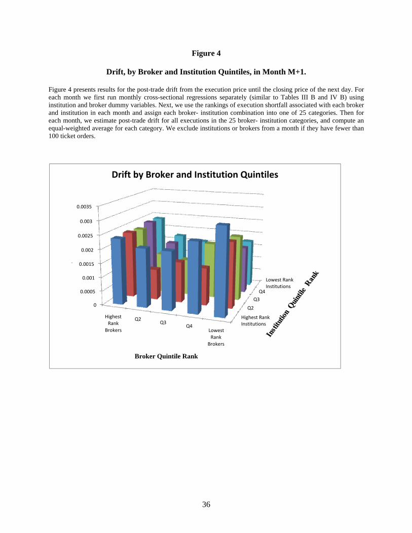
In Figure 4, we report the patterns in post-trade drift in Month M+1, by quintile intersection

(5×5) portfolio. For the top three broker quintiles (Quintiles 1 to 3), the difference in post-trade price drift

between the best and the worst performing institutions is not statistically significant. For broker quintile 4

and 5, the difference is statistically significant but inconsistent with the trading style hypothesis. That is,

the best institutions exhibit larger post-trade price drift than the worst institutions. We therefore fail to

find support for the hypothesis that trading cost persistence is explained by the institution’s style.

6. Determinants of Performance

What could account for persistent differences in trading cost across institutional desks? One

possible explanation is that different institutional desks trade different stocks, some of which are more

difficult to execute than others. However, our control regressions attempt to provide reasonable controls

for ticket attributes, stock characteristics and market conditions that affect trading cost.20

A second explanation is that some institutions pay higher commissions on their trades and receive

superior execution from their brokers. As a result, the benefits of the broker’s skill in executing the trades

is reflected in differences in the institution’s execution costs but the broker captures the surplus and the

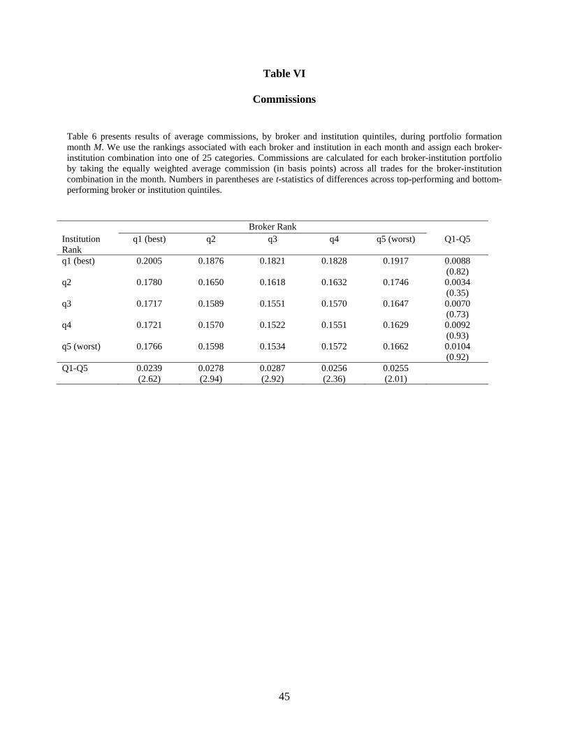
institution is no better off. The ANcerno data provides information on brokerage commission associated

with each ticket. In Table VI, we report average brokerage commissions in basis points, by quintile

intersection (5×5) portfolios, formed during portfolio formation month (similar to Table III, Panel B).

Several important patterns are observed in Table VI. Within any institutional quintile, we observe

20 As a robustness check, we run the persistence analysis separately for stocks classified as large cap (size quintile 4 and 5) and small cap and find similar results for both groups. For small cap stocks in month M+1, the performance difference for institutional desk quintiles is 66 basis points and for broker quintiles is 25 basis points. Our results are similar when we construct decile (instead of quintile) portfolios. In month M+1 (M+4), the difference between the best and the worst client declines and broker deciles are 84 (74) basis points and 38 (32) basis points, respectively.

23

that the pattern in commissions across broker quintiles has a U-shape. If commission payments drive

brokers to perform better, we expect commissions to decline monotonically from the top-performing to

the bottom-performing broker. The commission patterns are not consistent with this explanation. Neither

does the evidence support the explanation that broker incentive is driven by soft dollar arrangements

between institutions and brokerage firms. Conrad, Johnson and Wahal (2001) show that soft dollar

brokers provide worse executions relative to other brokers but also charge more commission than other

brokers. But, from Table VI, we see that quintile 5 brokers receive the same (not higher) commissions as

other groups and the difference in commissions between top and bottom brokers is not significant for any

institutional quintile. The bottom brokers in our sample do not appear to be predominantly soft dollar

brokers.21 Moreover, we observe performance persistence for both good and bad brokers.

The patterns suggest that the commission paid by the institution depend on the service received

from the brokers. Within broker quintiles, the commissions decline monotonically from top to bottom (the

t-statistic is greater than 2 for all broker quintiles). If commissions reflect the broker’s effort, one

explanation for persistence institutional patterns is the institution’s preference for low ‘touch’ versus high

‘touch’ executions. Goldstein, Irvine, Kandel and Weiner (2008) report that, in response to ECN

competition, full-service brokers now provide a full range of services ranging from low commission (or

‘touch’) executions such as direct access, dark pools and smart routers to high commission executions

such as a sales team working an order or the dealer posting their own capital to facilitate the trade. From

Table VI, it appears that bottom-performing institutions specify low touch execution venues, perhaps

reflecting a focus on explicit costs (commissions). Our evidence suggests that these alternatives can

ultimately cost institutions considerably more in price impact (60 basis points, from Table III) than the

explicit savings in commissions (3 basis points, from Table VI).

A third explanation is focused more on economic incentives and that skill in execution is partly

determined by broker effort. Such effort could be related to institutional client size and loyalty. The

21 A possible explanation is that soft dollars could be more directly associated with particular types of brokers during the mid-nineties period examined by Conrad, Johnson and Wahal (2001). Such a classification is more difficult in recent periods as the majority of brokers offer multiple commission contracts.

24

largest institutions are important clients generating large total revenues for the broker. Anecdotally, large

institutions such as T. Rowe Price and Fidelity are known to punish brokers by withholding business if

they feel the broker is leaking information about their trading patterns to the market. Brokers could put up

more of their own capital to lower the execution costs of large clients, or brokers could expend greater

effort in searching for low-cost counterparties for these clients, actions that suggest larger institutions

would receive better execution. Similarly, loyalty may result in greater broker effort.

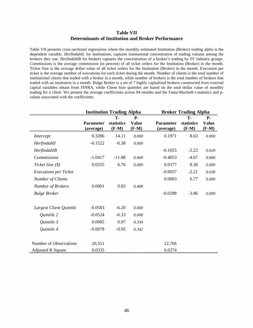
6.1. Cross-sectional regression of institutional performance

To test these ideas, we regress the trading alphas observed for institutions during the portfolio

formation month M (i.e., institutional effects from Table III) on a set of explanatory variables we create to

capture the determinants of institutional performance. In Table VII, we report the average coefficients

across the 84 monthly regressions and the Fama-Macbeth t-statistics and p-values. Consistent with Table

VI, we find that the institutional trading alpha is significantly negatively related to average commissions

paid by the institution, suggesting that higher explicit compensation to brokers is associated with better

execution performance. This is an interesting contrast to the findings in the mutual fund literature that

higher explicit compensation to money managers (in the form of higher management fees) is associated

with lower fund performance (Gil-Bazo and Ruiz-Verdu (2009)).

We also find that the dollar size of the ticket is positively related to trading cost, suggesting that

larger orders are more difficult to execute and more likely to face greater scrutiny from potential

counterparties. We estimate the variable HerfindahlI, calculated as an institutions’ monthly Herfindahl

index of trading market share across brokers. A higher value of HerfindahlI reveals that the institution

concentrates their order flow with fewer brokers. In Table VII, the significantly negative coefficient on

HerfindahlI suggests that institutions that concentrate trading receive better execution. Concentrating

trades with few brokers may help lower the risk of leakage while the ticket is being worked and reduce

the front running cost. Finally, since the institution’s identity is unknown, we proxy for institution size

based on the dollar volume of monthly transactions executed by the institution, and form institutional

25

volume quintile portfolios. Consistent with an institution size effect, we find that the trading desks of

large institutions are associated with better performance.

The last explanation that we consider is that some buy-side and sell-side trading desks possess

superior ability. These abilities could take the form of generally trading against the prevailing market

momentum, so that traders in effect are paid for the liquidity they provide rather than having to pay for

the liquidity they demand. Essentially this is a market timing skill. Certain institutions send orders when

the pool of potential counterparties is large or respond quickly to order imbalances. These institutions

benefit from lower execution costs, or in the case of best institutions, earn the liquidity mark-up when

demand for immediacy is high. In unreported results, we observe that the greatest effect on institutional

performance in Table VII comes from the omitted variable Momentum. This variable is omitted because

our research design removes the effects of momentum on a ticket-by-ticket basis in Table IV, Panel A.

However, when we remove this variable from our control regression and instead use it as an explanatory

variable in this regression, Momentum has a significant positive coefficient that can increase the

regression R2 markedly. That is, institutions which consistently trade stocks in the direction of momentum

are demanding liquidity when it is scarce and this liquidity demand significantly raises their trading cost.

6.2. Cross-sectional regression of broker performance

To aid institutions in broker selection, we report on characteristics that are systematically

associated with broker performance. The second column in Table VII presents several variables that

reliably predict performance differences across brokers. Larger brokers may have access to greater

networks of counterparties than smaller brokers (Onaran (2007)). They may also be able to purchase the

services of highly-skilled traders. Yet larger brokers have more clients and it is not clear how these

resources would be allocated to particular clients. Small brokers may expend greater effort and secure

superior execution for particular clients because these clients are important to them. This is the argument

made in Goldstein et al. (2008) who contend that institutions pay premium (relative to ECN execution)

commissions in return for a package of broker services, one of which is trading cost minimization. In their

26

argument it is the strength of the client-broker relationship that determines a broker’s effort on behalf of a

client. The strength of this relationship is determined by the importance to that broker of the client’s

revenue stream. This argument confounds a simple relationship between broker or institutional size and

execution performance.

The results for average commissions and the average ticket size are similar to those observed in

the institutional regressions. The number of executions per ticket is negatively related to broker trading

alpha, implying that trading costs decline when the broker expends more effort in breaking the large ticket

into smaller pieces for execution. To capture the extent of broker specialization by industry or sector, we

estimate the variable HerfindahlB, a brokers’ Herfindahl index of the trading volume market share across

Fama-French industry groups.22 The negative coefficient on HerfindahlB shows that brokers that

specialize in sectors or industries have lower execution costs. One possible explanation for institutional

performance is their sophistication in routing orders to specialized boutique brokers.

Finally, we gathered annual data on broker Capital from the Financial Industry Regulatory

Association (FINRA) to identify bulge bracket brokers (Bulge broker) as those most likely to have capital

available to facilitate their clients’ execution. These seven brokers are capitalized with at least twice as

much available capital as their nearest competitors with capital ranging from a minimum of $18 billion

for Bear Stearns in 1999 to a maximum of $150 billion for Merrill Lynch in 2005.23 The best capitalized

brokers have significantly better performance suggesting that their capital, and the ability to provide a

direct counterparty for difficult to execute trades, represents a difficult to replicate competitive

advantage.24

22 Brokers can differ in their degree of specialization. At one extreme, the generalist brokers offer execution services in a wide variety of stocks and serve as a convenient one-stop shop for clients. At the other extreme, boutique brokers such as Freeman, Billings and Ramsey, specialize in executing stocks in select industries. HerfindahlB is a proxy for broker specialization by industry. We thank Tim McCormick for suggesting the line of investigation. 23 Broker capital is defined as shareholder’s equity plus subordinated debt. The 7 bulge bracket brokers are Merrill Lynch, Goldman Sachs, Morgan Stanley, Citigroup, Lehman Brothers, Bear Stearns and, after their 2000 merger with DLJ, Credit Suisse First Boston. 24 However, we stress that the negative relation between broker capital and trading cost is not monotonic throughout our broker sample as several lightly capitalized brokers also have superior execution performance.

27

6.3. Is the institution’s choice of broker sensitive to past execution quality?

If some brokers are persistently bad, then why do they survive? There is a similar debate in the

mutual fund literature on why poorly performing index funds or money market funds survive. Elton,

Gruber and Busse (2004) examine S&P 500 index funds and report that the difference in risk across funds

is small and the difference in returns is easy to forecast. Yet a large amount of new investor funds goes to

the poorest-performing index funds leading them to conclude that many investors seem to be making

decisions that violate rationality. Further, in a market where arbitrage is impossible, they note that all that

is necessary for a dominated product (or service, in this case) to exist and even prosper is a set of

uninformed participants.

In the context of our study, the worst performing brokers can survive because some institutions

are either performance-insensitive or face substantial information gathering costs. Institutional barriers to

order flow (for example, endowments mandated to trade through custody banks), capacity limitations at

good brokerage houses, or agency conflicts can also serve as explanations.25 Another explanation is that

institutions use order flow to purchase a package of non-execution related services, which would

otherwise be expected to be paid more explicitly. Examples of non-execution related arrangements

include prime brokerage services such as securities lending and borrowing, allocations in hot IPOs, and

access to research reports by sell-side analysts.

We examine whether the worst performing brokers get penalized and the best performing brokers

get rewarded in future periods. For each institution, we identify the ten brokers with the highest trading

volume market share with the institution over a six-month ranking period (top 10 brokers). We relate the

execution shortfall with the propensity for a top 10 broker to retain their status during the next six months

(the observation period). The best performing brokers during the ranking period have a 66 percent chance

of retaining the top 10 status in the observation period. In contrast, the worst performing brokers have a

25 For example, the Securities and Exchange Commission (SEC) fined Fidelity investments $8 million in March 2008. The SEC alleged that Fidelity had directed trading business to certain brokerages, not because of superior service, but because the brokers had enticed Fidelity traders with gifts. The case led to an industry wide probe of gift-giving practices.

28

60 percent chance of retaining their top 10 status (p-value of difference < 0.01). We also examine the

propensity for a non-top 10 broker during the ranking period to achieve a top 10 status in the observation

period. The best (worst) performing brokers exhibit a likelihood of 6.49 percent (6 percent) of achieving

top 10 status in the observation period (p-value of difference < 0.01).

Finally, we examine the change in market share of brokers from ranking to observation period.

For brokers ranked in the top two performing quintiles, we see an increase in market share, from 12.95 to

13.32 percent for top quintile and from 22.86 to 23.32 percent for quintile 2. In contrast, brokers ranked in

the two worst performing quintiles see a decrease in market share, from 25.12 to 24.78 percent for

quintile 4 and from 14.38 to 13.97 percent for worst quintile. Although we examine a relatively short

window, the results indicate that routing decisions are sensitive to past performance, suggesting that

institutions relate performance differences to broker skill and not simply ticket difficulty.26 We conclude

that the worst performing brokers lose market share slowly.

7. Conclusion

We contribute to the literature on the performance of institutional trading desks, an important

category of financial intermediaries who are responsible for trillions of dollars in trade executions each

year. We examine institutional equity transactions using data provided by ANcerno Ltd., a consulting

firm that works with institutional investors to monitor their equity trading costs. Our tests examine

whether past performance is informative about future performance. Our main finding is that institutional

trading desks can sustain relative performance over adjacent periods. The results support the existence of

skilled traders who can help create positive (investment) alpha through their trading activities. We also

find that some brokers can deliver better executions over time and that the combined effects of the

institutional desk and the broker are large. We identify a set of trading decisions that are related to

performance.

26 The results are consistent with those reported by Boehmer, Jennings and Wei (2007), who examine the impact on order flow of SEC Rule 11Ac1-5 (Dash 5 reports), which mandates U.S. market centers to publish a broad set of standardized execution-quality metrics each month.

29

These findings have implications for several strands of research. To our knowledge, we provide

the first evidence of performance persistence of buy-side trading desks and sell-side brokers, and assess

the contributions of the brokers and institutional desks in a single framework. These results contribute to

the literature on performance of financial intermediaries. The study also contributes to the literature

suggesting that mutual funds can sustain relative performance beyond expenses or momentum over

adjacent periods. Our findings suggest that trading cost is a source of fund performance persistence.

The cumulative dollar impact of the trading cost difference is large – an approximate calculation

suggests that the annual trading cost reductions exceed $1 billion if institutions route order flow to the

best performing brokers instead of the worst performing brokers.27 While this estimate is no doubt

imprecise, the magnitude of the estimate emphasizes that broker selection based on past performance

represents an important dimension of the money manager’s fiduciary obligation. However, because

brokers provide a package of non-execution related services to institutions, we cannot necessarily

conclude from this analysis that institutions have violated the best execution obligations to their investors.

One caveat should be noted. Since we do not know the identity of the institutions in our data, we

cannot independently determine the size of the institution and the institution’s turnover rate. Thus, trading

activity in our data cannot be directly translated into mutual fund abnormal returns. All that we can note is

that, given the average mutual fund turnover rate, which can approach 100 percent annually (Edelen et al.

(2007)), the persistent difference in trading cost that we estimate can explain a portion of the fund

performance reported in the existing literature.

27 A worst performing broker in our sample executes roughly $700 million each month, or $8.4 billion annually. In a typical month, the worst broker quintile has approximately 50 brokers. Thus, brokers in the bottom quintile execute roughly $420 billion each year. In Table IV, Panel B, we estimate trading cost difference of approximately 28 basis points per ticket between the best and the worst broker quintiles. If institutions route orders to the best brokers instead of the worst brokers, the estimated trading cost reduction is $1.18 billion. A similar approach can be used to estimate dollar amounts for other broker quintiles. Moreover, these amounts understate the importance of broker selection since our sample contains only a portion of the institutional order flow. We note that the savings from institutional desk performance would be even larger.

30

References Berkowitz, S., D. Logue, and E. Noser, 1988, The Total Cost of Transactions on the NYSE, Journal of Finance, 43, 97-112. Boehmer, E., R. Jennings and L. Wei, 2007. Public disclosure and private decisions: Equity market execution quality and order routing, Review of Financial Studies, 20, 315-358.

Baks, K., 2006. On the performance of mutual fund managers, working paper, Emory University.

Bessembinder, H., and H. Kaufman. 1997. “A comparison of trade execution costs for NYSE and NASDAQ-listed stocks.” Journal of Financial and Quantitative Analysis, 32, 287-310.

Bessembinder, H., M. Panayides and K. Venkataraman, 2009, Hidden Liquidity: An analysis of order exposure strategies in electronic stock markets, working paper, Journal of Financial Economics, forthcoming.

Bollen, N., and J. Busse, 2005. Short-term persistence in mutual fund performance, Review of Financial Studies, 18, 569-597.

Busse, J., and P. Irvine, 2006. Bayesian alphas and mutual fund performance, Journal of Finance, 61, 2251-2288.

Carhart, M., 1997. On persistence in mutual fund performance, Journal of Finance, 52, 57-82.

Chan L., and J. Lakonishok, 1995. The behavior of stock prices around institutional orders, Journal of Finance, 50, 713-735.

Chemmanur, T., S. He, and G. Hu, 2009. The role of institutional investors in seasoned equity offerings, Journal of Financial Economics, forthcoming.

Chiyachantana, C., Jain P., Jiang C., and R. Wood, 2004. International evidence on institutional trading behavior and the determinants of price impact, Journal of Finance, 59, 865-894.

Christoffersen, S., Keim, D., and D. Musto, 2006. Valuable information and costly liquidity: Evidence from individual mutual fund trades, working paper, McGill University.

Conrad, J., K. Johnson, and S. Wahal 2001. Institutional trading and soft dollars, Journal of Finance, 46, 397- 416.

Edelen, R., Evans, R., and G.B. Kadlec, 2007, Scale effects in mutual fund performance; The role of trading costs, working paper, University of California, Davis.

Elton, E., M. Gruber, and J. Busse, 2004, Are investors rational? Choices among index funds, Journal of Finance, 59, 261–288. Gil-Bazo, J., and P.Ruiz-Verdu, 2009, The relation between price and performance in the mutual fund industry, Journal of Finance, forthcoming.

Goldstein, M., Irvine, P., Kandel, E., and Z. Weiner, 2008. Brokerage commissions and institutional trading patterns, forthcoming, Review of Financial Studies.

31

Griffin, J., J. Harris and S. Topaloglu, 2003, The Dynamics of Institutional and Individual Trading, Journal of Finance, 58, 2285-2320.

Grinblatt, M., and S. Titman, 1989, Mutual Fund Performance: An Analysis of Quarterly Portfolio Holdings, Journal of Business, 62, 393-416. Harris, L., 1997, Order Exposure and Parasitic Traders, Working Paper, Marshall School of Business.

Hu, G., 2005. Measures of implicit trading costs and buy-sell asymmetry, working paper, Babson College.

Huang, R., and Stoll, H. 1996. Dealer versus auction markets: A paired comparison of execution costs on NASDAQ and NYSE. Journal of Financial Economics, 41, 313-357.

Jensen, M. 1968. The performance of mutual funds in the period 1945-64, Journal of Finance 23, 389-416.

Jones, C., and M. Lipson, 2001. Sixteenths: Direct evidence on institutional trading costs, Journal of Financial Economics, 59, 253-278.

Kacperczyk, M., and A. Seru, 2007. Fund manager use of public information: New evidence of managerial skill, Journal of Finance, 62, 485-528.

Kacperczyk, M., C. Sialm, and L. Zheng, 2008, Unobserved actions of mutual funds, Review of Financial Studies, 21(6), 2379-2416.

Keim, D., 1999. An analysis of mutual fund design: the case of investing in small cap stocks, Journal of Financial Economics, 51, 173-194.

Keim D., and A. Madhavan, 1995. Anatomy of the trading process: Empirical evidence on the behavior of institutional traders, Journal of Financial Economics, 37.

Keim D., and A. Madhavan, 1997. Transactions costs and investment style: An inter-exchange analysis of institutional equity trades, Journal of Financial Economics, 46, 265-292.

Lee, C., and M. Ready, 1991, Inferring Trade Direction from Intraday Data, Journal of Finance, 41, 733-746.

Linnainmaa, J., 2007. Does it matter who trades? Broker identities and the information content of stock trades, working paper, University of Chicago.

Lipson, M., and A. Puckett, 2007, Volatile Markets and Institutional Trading, working paper, University of Missouri.

Macey, J.R., and M. O’Hara, 1997, The law and economics of best execution, Journal of Financial Intermediation, 6, 188-223. Madhavan, A., Cheng, M., 1997, In search of liquidity: block trades in the upstairs and downstairs Market, Review of Financial Studies 10, 175–203. Madhavan, 2002. VWAP Strategies, Transaction Performance, Spring 2002.

32

Onaran, Y., 2007. The world’s best brokers, Bloomberg Markets, June 2007, 74-79.

Perold, A., 1988. The implementation shortfall: Paper versus reality, Journal of Portfolio Management, 14, 4-9.

Sofianos, G., 2001. The changing NASDAQ market and institutional transaction fees, Goldman Sachs derivatives and trading research, May 31.

Sofianos, G., 2005. Execution quality benchmarks: I can see clearly now…, Trading and Market Structure Analysis, Goldman Sachs.

Stoll, H., 2000, Friction, Journal of Finance, 55, 1479-1514. Wagner, W., and M. Edwards, 1993. Best execution, Financial Analysts Journal 49, 65–71.

Wermers, R., 2000, Mutual Fund Performance: An Empirical Decomposition into Stock-Picking Talent, Style, Transactions Costs, and Expenses, Journal of Finance, 55, 1655-1703.

33

Figure 1: Institutional and Broker Trading Alphas Figure 1 presents the monthly time series of Trading Alphas, by quintiles formed in portfolio formation month, for institutional trading desks (Panel A) and brokers (Panel B). The estimates are obtained from Tables III B and IV B. Panel A

Panel B

‐0.4

‐0.2

0

0.2

0.4

0.6

0.8

Portfolio Formation month

M+1 M+2 M+3 M+4

1 (Highest Rank Institutions) Institution Quintile 2

Institution Quintile 3 Institution Quintile 4

5 (Lowest Rank Institutions)

‐0.4

‐0.2

0

0.2

0.4

0.6

0.8

Portfolio Formation month

M+1 M+2 M+3 M+4

1 (Highest Rank Brokers) Broker Quintile 2 Broker Quintile 3

Broker Quintile 4 5 (Lowest Rank Brokers)

34

Figure 2: Trading Volume Market Share

Figure 2, Panel A presents the proportion of dollar trading volume routed by an institution quintile to each broker quintile. Panel B presents the proportion of dollar trading volume of each broker quintile that is attributable to each institutional client quintile. Institutional and Broker quintile rankings are based on independent trading alpha estimates described earlier in Tables III B and IV B. Rankings as well as the dollar volume are measured contemporaneously.

A. Trading Volume Market Share of Institutions, by Broker Quintiles

B. Trading Volume Market Share of Brokers, by Institution Quintiles

0.00%

5.00%

10.00%

15.00%

20.00%

25.00%

30.00%

35.00%

40.00%

1 (Highest Rank Institutions)

2 3 4 5 (Lowest Rank Institutions)

Highest Rank Brokers Quinti le 2 Brokers Quinti le 3 Brokers Quinti le 4 Brokers Lowest Rank Brokers

0.00%

5.00%

10.00%

15.00%

20.00%

25.00%

30.00%

35.00%

40.00%

45.00%

50.00%

1 (Highest Rank Brokers)

2 3 4 5 (Lowest Rank Brokers)

Highest Rank Institutions Quinti le 2 Institutions Quinti le 3 Institutions Quinti le 4 Institutions Lowest Rank Institutions

35

Figure 3

Trading Alpha, by Broker and Institution Quintiles, in Month M+1.

Figure 3 presents results for Trading Alpha by Broker and Institution Quintile. For each month we first run monthly cross-sectional regressions separately (similar to Tables III B and IV B) using institution and broker dummy variables. Next, we use the rankings associated with each broker and institution in each month and assign each broker-institution combination into one of 25 categories. Then for each month, we estimate regressions using the execution shortfall as the dependent variable, and the control variables described earlier as well as the 25 broker-institution combination dummies as the independent variables (this specification excludes individual broker and institution dummy variables). We use each month’s broker-institution combination ranking in month M to estimate similar regression for the next month. Our methodology produces 25 coefficient estimates (that represent all possible institution-broker rank combinations) for the formation month (month M) and the subsequent month (month M+1). We report the coefficients estimated for the subsequent month for all 25 fractile categories in Figure 3.

36

Figure 4

Drift, by Broker and Institution Quintiles, in Month M+1.

Figure 4 presents results for the post-trade drift from the execution price until the closing price of the next day. For each month we first run monthly cross-sectional regressions separately (similar to Tables III B and IV B) using institution and broker dummy variables. Next, we use the rankings of execution shortfall associated with each broker and institution in each month and assign each broker- institution combination into one of 25 categories. Then for each month, we estimate post-trade drift for all executions in the 25 broker- institution categories, and compute an equal-weighted average for each category. We exclude institutions or brokers from a month if they have fewer than 100 ticket orders.

Highest Rank Institutions

Q2

Q3

Q4

Lowest Rank Institutions

0

0.0005

0.001

0.0015

0.002

0.0025

0.003

0.0035

Highest Rank 

Brokers

Q2 Q3

Q4Lowest Rank 

Brokers

Drift

Broker Quintile Rank

Drift by Broker and Institution Quintiles

37

Table I Descriptive Statistics

This table reports the descriptive statistics for our sample of institutional trades from ANcerno Ltd. for the period from January 1, 1999 to December 31, 2005. We use a ticket as our level of analysis. A ticket could be executed through multiple trades. We further restrict the sample to tickets that are executed by clients with at least 100 tickets during a particular month, as well as to tickets executed on NYSE/NASDAQ stocks. We present the results for the full sample, as well as by disaggregating the sample based on year, order direction, and firm size quintiles. Firm size quintiles are based on the stocks in our sample. Execution shortfall is measured for buy tickets as the execution price minus the market price at the time of ticket placement divided by the market price at ticket placement (for sell tickets we multiply by -1). Commissions are reported in dollars per share. We report the volume weighted averages for execution shortfall and commissions.

Number

of Brokers Number of Institutions

Number of

Stocks Number of tickets

Ticket Size

Ticket Size/Average daily volume

(30 days)

Number of executions per ticket

Execution Shortfall

Commissions ($/share)

Panel A: Full sample 1137 664 7,589 34,885,972 17,366 2.4% 1.51 0.26 0.028

Panel B: By year

1999 670 323 5,671 3,340,323 24,088 4.8% 1.31 0.35 0.017 2000 654 321 5,442 4,449,647 23,290 3.6% 1.27 0.34 0.016 2001 686 335 4,673 5,173,781 22,583 2.7% 1.28 0.37 0.018 2002 711 358 4,365 5,725,588 15,901 2.1% 1.51 0.16 0.041 2003 681 319 4,286 5,375,277 13,666 1.8% 1.59 0.20 0.045 2004 623 307 4,358 5,548,414 12,889 1.6% 1.49 0.17 0.040 2005 633 286 4,237 5,272,942 13,067 1.7% 1.99 0.17 0.031

Panel C: Order direction Sell 15,844,002 19,468 2.6% 1.55 0.39 0.028 Buy 19,041,970 15,618 2.3% 1.48 0.13 0.029

Panel D: Firm size (quintiles)

Small 58,377 8,932 33.8% 1.21 1.03 0.016 2 401,147 9,213 23.3% 1.30 0.56 0.022 3 1,961,381 8,400 8.9% 1.37 0.40 0.026 4 6,352,644 9,129 3.8% 1.37 0.27 0.029

Large 26,112,423 20,188 1.2% 1.56 0.26 0.028

38

Table II Performance of Institutional Trading Desks

Table 2 examines the performance persistence of institutional trading desks. The trades in the sample are executed by 664 institutions during the time period from January 1, 1999 to December 31, 2005. Only institutions with 100 or more tickets in a month are included in the analysis. Execution shortfall is measured for buy tickets as the execution price minus the market price at the time of ticket placement divided by the market price at ticket placement (for sell tickets we multiply by -1). We calculate the average execution shortfall across the ticket for each institution each month. At the end of the each month, we form institutions into quintile portfolios based on execution cost for the month. We report the average (equal-weighted) execution shortfall for these quintiles in the portfolio formation month and the next four months. We also include the percentage of institutions that end up in the same quintile during subsequent months (Retention %) and the average percentile rank of quintile institutions (Percentile). All numbers are in percent. Numbers in parentheses are t-statistics.

MonthsCurrent Quarter Performance Quintiles

Portfolio Formation

month M+1 M+2 M+3 M+4

Q1 Exec. Shortfall -0.408 -0.072 -0.061 -0.056 -0.043 Retention % 100.00 46.15 44.88 44.50 43.25 Percentile 10.62 31.91 32.49 32.71 33.12

Q2 Exec. Shortfall 0.033 0.146 0.149 0.153 0.155 Retention % 100.00 28.91 27.27 27.49 26.99 Percentile 30.55 42.52 43.22 43.53 43.60

Q3 Exec. Shortfall 0.254 0.266 0.271 0.263 0.264 Retention % 100.00 25.96 28.64 27.34 26.83 Percentile 50.55 50.90 50.98 50.70 51.04

Q4 Exec. Shortfall 0.486 0.383 0.376 0.373 0.365 Retention % 100.00 28.43 28.01 28.34 26.11 Percentile 70.51 58.36 57.95 57.61 57.21

Q5 Exec. Shortfall 0.979 0.615 0.599 0.590 0.583 Retention % 100.00 45.29 44.04 44.12 42.58 Percentile 90.43 68.89 67.88 67.73 67.27 Q5 – Q1 (Trading Alpha) 1.39 0.69 0.66 0.65 0.63 (169.08) (57.07) (53.43) (51.32) (49.71)

39

Table III, Panel A Institution Fixed Effect Regressions of Execution Shortfall on Economic Determinants of

Trading Cost

This table reports coefficient estimates from monthly institution fixed-effects regression of execution shortfall on economic determinants of execution shortfall. The model is estimated for each of the 84 month in our sample. We present the average coefficients across 84 months and the Fama-Macbeth t-statistics and p-values associated with the coefficients. We also report the proportion of coefficients that are positive. Daily return, daily S&P return, daily volume and market values are obtained from the CRSP database. The Buy dummy equals 1 for buy orders and 0 for sell orders. The order direction is given in the ANcerno database. Order imbalance is the dollar imbalance on the day prior to the day a ticket is executed. The dollar imbalance is calculated using TAQ data, and is defined as the difference of the dollar volume of buyer initiated trades and the dollar volume of seller initiated trades, divided by the total dollar volume of buyer and seller initiated trades. Trades are assigned as buyer or seller initiated using the Lee-Ready (1991) algorithm. Momentum is measured using the stock’s return on the day prior to the ticket execution date. The return is obtained from the daily CRSP database. All explanatory variables are demeaned each month so that each institution coefficient measures the execution shortfall for an average order for the client.

Parameter (average)

T-statistics (F-M)

P-Value (F-M)

Positive coefficients

(%)

Number of months 84

Stock Volatility (Absolute value of daily return) 0.03442 20.56 0.000 0.98 Market Volatility (Absolute value of daily S&P 500 return) -0.01885 -3.92 0.000 0.35

Buy dummy -0.00072 -2.72 0.008 0.37

Order imbalance (previous trading day, $) -0.00024 -1.62 0.108 0.48 Order imbalance (previous trading day, $) * Buy dummy 0.00015 0.54 0.593 0.45

Momentum (Previous day's return) -0.01835 -7.36 0.000 0.11

Momentum (Previous day's return) * Buy dummy 0.03367 7.69 0.000 0.87

Log (Average previous 30 day daily volume) -0.00023 -8.20 0.000 0.23

Log Market value (as of the beginning of month) 0.00009 3.28 0.002 0.68 NYSE stock dummy (only NYSE and NASDAQ stocks included) -0.00042 -8.04 0.000 0.14

1/Price 0.00585 8.49 0.000 0.86

Ticket Size/Average previous 30 day daily volume 0.00033 3.85 0.000 0.69

Adjusted R Square 0.0299

40

Table III, Panel B Persistence in Monthly Institution Trading Alpha

Table 3, Panel B examines the persistence of monthly institutional Trading Alpha. The trades in the sample are placed by 664 different institutions during the time period from January 1, 1999 to December 31, 2005. Trading Alpha is estimated for each institution in each month using the cross-sectional regression presented in Panel A. All independent variables are de-meaned and our regression includes dummy variables for each institution. The coefficient estimate on institution dummy variables is the institution’s Trading Alpha. Each month we divide all institutions into five quintiles based on their Trading Alpha estimates. We then report the average (equal-weighted) Trading Alpha for these quintiles for the portfolio formation months and the next four months. We also include the percentage of institutions that end up in the same quintile during subsequent months (Retention %) and the average percentile rank of quintile institutions (Percentile). We exclude an institution from a month if it has fewer than 100 ticket orders. All returns are in percent. Numbers in parentheses are t-statistics.

MonthsCurrent Quarter Performance Quintiles

Portfolio Formation

month M+1 M+2 M+3 M+4

Q1 Trading Alpha -0.311 -0.146 -0.133 -0.130 -0.122 Retention % 100.00 55.97 54.23 53.10 52.08 Percentile 10.62 25.87 27.22 27.68 28.18

Q2 Trading Alpha 0.022 0.084 0.078 0.080 0.085 Retention % 100.00 32.13 32.96 31.25 29.91 Percentile 30.54 41.32 41.32 41.95 42.34

Q3 Trading Alpha 0.174 0.170 0.176 0.173 0.168 Retention % 100.00 32.63 32.69 31.65 29.59 Percentile 50.55 50.74 51.17 51.43 51.40

Q4 Trading Alpha 0.321 0.271 0.261 0.253 0.246 Retention % 100.00 33.55 31.44 30.10 30.33 Percentile 70.52 60.78 60.10 59.33 58.81

Q5 Trading Alpha 0.653 0.471 0.448 0.442 0.436 Retention % 100.00 53.97 51.61 50.75 50.90 Percentile 90.39 73.89 72.61 71.98 71.61 Q5 – Q1 (Trading Alpha) 0.96 0.62 0.58 0.57 0.56 (141.48) (69.35) (63.42) (61.24) (58.90)

41

Table IV, Panel A Broker Fixed Effect Regressions of Execution Shortfall on Economic Determinants of

Trading Cost

This table reports coefficient estimates from monthly broker fixed-effects regression of execution shortfall on economic determinants of execution shortfall. The model is estimated for each of the 84 month in our sample. We present the average coefficients across 84 months, and the Fama-Macbeth t-statistics and p-values associated with the coefficients. We also report the proportion of coefficients that are positive. Daily return, daily S&P return, daily volume and market values are obtained from the CRSP database. The Buy dummy equals 1 for buy orders and 0 for sell orders. The order direction is given in the ANcerno database. Order imbalance is the dollar imbalance on the day prior to the day a ticket is executed. The dollar imbalance is calculated using TAQ data, and is defined as the difference of the dollar volume of buyer initiated trades and the dollar volume of seller initiated trades, divided by the total dollar volume of buyer and seller initiated trades. Trades are assigned as buyer or seller initiated using the Lee-Ready (1991) algorithm. Momentum is measured using the stock’s return on the day prior to the ticket execution date. The return is obtained from the daily CRSP database. All explanatory variables are demeaned each month so that each broker coefficient measures the execution shortfall for an average order for the broker.

Parameter (average)

T-statistics (F-M)

P-Value (F-M)

Positive coefficients

(%)

Number of months 84

Stock Volatility (Absolute value of daily return) 0.03603 21.73 0.000 0.98

Market Volatility (Abs. value of daily S&P 500 ret) -0.01952 -4.01 0.000 0.33

Buy dummy -0.00076 -2.80 0.006 0.38

Order imbalance (previous trading day, $) -0.00025 -1.69 0.094 0.50

Order imb (previous trading day, $) * Buy dum 0.00026 0.92 0.358 0.46

Momentum (Previous day's return) -0.02010 -7.88 0.000 0.10

Momentum (Previous day's return) * Buy dummy 0.03714 8.21 0.000 0.88

Log (Average previous 30 day daily volume) -0.00027 -9.65 0.000 0.18

Log Market value (as of the beginning of month) 0.00017 6.74 0.000 0.75 NYSE stock dummy (only NYSE and NASDAQ stocks included) -0.00070 -10.09 0.000 0.06

1/Price 0.00527 8.05 0.000 0.83

Ticket Size/Average previous 30 day daily volume 0.00048 4.89 0.000 0.75

Adjusted R Square 0.0249

42

Table IV, Panel B Persistence of Monthly Broker Trading Alpha

Table 4, Panel B examines the persistence of monthly broker Trading Alpha. The sample includes all trades by 431 different brokerage firms that executed at least 100 trades in a month during the time period from January 1, 1999 to December 31, 2005. Trading Alpha is estimated for each brokerage firm in each month using the broker fixed effects regression presented in Panel A. All independent variables are de-meaned and our regression includes dummy variables for each brokerage firm. The coefficient estimate on brokerage firm dummy variables is the brokerage firm’s Trading Alpha. Each month we divide all brokerage firms into five quintiles based on their Trading Alpha estimates. We then report the average (equal-weighted) Trading Alpha for these quintiles for the portfolio formation months and the next four months. We also include the percentage of brokerage firms that end up in the same quintile during subsequent months (Retention %) and the average percentile rank of quintile brokerage firms (Percentile). All returns are in percent. Numbers in parentheses are t-statistics.

MonthsCurrent Quarter Performance Quintiles

Portfolio Formation

month M+1 M+2 M+3 M+4

Q1 Trading Alpha -0.314 -0.007 0.004 0.007 0.003 Retention % 100.00 42.93 41.26 39.83 41.46 Percentile 10.76 37.26 37.86 38.91 38.20

Q2 Trading Alpha 0.069 0.150 0.147 0.147 0.143 Retention % 100.00 27.98 26.93 26.27 26.97 Percentile 30.56 46.79 47.12 46.90 47.12

Q3 Trading Alpha 0.193 0.208 0.184 0.195 0.188 Retention % 100.00 28.63 28.75 26.83 27.91 Percentile 50.56 53.01 51.12 52.25 52.47

Q4 Trading Alpha 0.308 0.229 0.226 0.207 0.205 Retention % 100.00 27.59 27.77 26.94 26.69 Percentile 70.57 56.10 56.12 55.05 54.96

Q5 Trading Alpha 0.620 0.277 0.279 0.257 0.255 Retention % 100.00 34.68 35.17 33.17 32.87 Percentile 90.33 59.42 60.16 58.99 59.08 Q5 – Q1 (Trading Alpha) 0.93 0.28 0.28 0.25 0.25 (84.90) (20.61) (19.53) (17.99) (18.29)

43

Table V, Panel A Persistence in Institutional Trading Alpha within Broker Groups

Table 5 (Panel A) presents results for the persistence in institutional trading alpha, controlling for the execution quality of brokerage firms. For each month we first run monthly cross-sectional regressions separately (similar to Tables III B and IV B) using institution and broker dummy variables. Next, we use the rankings associated with each broker and institution in each month and assign each broker-institution combination into one of 25 categories. Then for each month, we estimate regressions using the execution shortfall as the dependent variable, and the control variables described earlier as well as the 25 broker-institution combination dummies as the independent variables (this specification excludes broker and client dummy variables). We use each month’s broker-institution combination ranking to estimate similar regression for the next 4 months. Our methodology produces 25 coefficient estimates (that represent all possible institution-broker rank combinations) for the formation month (t) and the subsequent four months. For each period and brokerage firm quintile, we hold the broker ranking constant and report the difference between the highest institutional quintile (quintile=1) and lowest institutional quintile (quintile=5). We exclude institutions or brokers from a month if they have fewer than 100 ticket orders. Numbers in parentheses are t-statistics.

Difference in Trading Alpha between Highest and Lowest Institutional

Quintile

Broker Quintile Rankings

Portfolio Formation

month M+1 M+2 M+3 M+4

q1 (best) 0.976 0.715 0.663 0.619 0.618 (33.62) (24.11) (21.36) (17.86) (18.17)

q2 0.796 0.502 0.4471 0.449 0.456 (36.96) (20.59) (27.50) (19.05) (20.70)

q3 0.784 0.489 0.492 0.466 0.426 (30.68) (21.80) (19.62) (19.36) (18.47)

q4 0.799 0.551 0.498 0.492 0.489 (30.13) (22.26) (22.02) (18.45) (17.94)

q5 (worst) 0.785 0.618 0.667 0.591 0.547 (18.24) (17.32) (15.29) (17.38) (16.02)

44

Table V, Panel B Persistence in Broker Trading Alpha within Institutional Groups

Table 5 (Panel B) presents results for the persistence in broker trading alpha, controlling for the execution quality of institutions. For each month we first run monthly cross-sectional regressions separately (similar to Tables III B and IV B) using institution and broker dummy variables. Next, we use the rankings associated with each broker and institution in each month and assign each broker-institution combination into one of 25 categories. Then for each month, we estimate regressions using the execution shortfall as the dependent variable, and the control variables described earlier as well as the 25 broker-institution combination dummies as the independent variables (this specification excludes broker and institution dummy variables). We use each month’s broker-institution combination ranking to estimate similar regression for the next 4 months. Our methodology produces 25 coefficient estimates (that represent all possible institution-broker rank combinations) for the formation month (t) and the subsequent four months. For each period and institution quintile, we hold the institution ranking constant and report the difference between the highest broker quintile (quintile=1) and lowest broker quintile (quintile=5). We exclude institutions or brokers from a month if they have fewer than 100 ticket orders. Numbers in parentheses are t-statistics.

Difference in Trading Alpha between Highest and Lowest Broker Quintile

Institution Quintile Rankings

Portfolio Formation

month M+1 M+2 M+3 M+4

q1 (best) 0.785 0.348 0.306 0.326 0.343 (22.66) (11.64) (8.89) (9.80) (11.27)

q2 0.619 0.261 0.246 0.212 0.209 (21.52) (11.32) (11.19) (8.84) (8.09)

q3 0.510 0.202 0.209 0.179 0.199 (19.42) (10.02) (9.97) (8.15) (9.39)

q4 0.556 0.208 0.246 0.225 0.220 (20.16) (9.29) (9.59) (8.77) (9.28)

q5 (worst) 0.603 0.251 0.310 0.296 0.272 (16.82) (9.17) (8.49) (9.72) (8.06)

45

Table VI

Commissions

Table 6 presents results of average commissions, by broker and institution quintiles, during portfolio formation month M. We use the rankings associated with each broker and institution in each month and assign each broker-institution combination into one of 25 categories. Commissions are calculated for each broker-institution portfolio by taking the equally weighted average commission (in basis points) across all trades for the broker-institution combination in the month. Numbers in parentheses are t-statistics of differences across top-performing and bottom-performing broker or institution quintiles.

Broker Rank Institution Rank

q1 (best) q2 q3 q4 q5 (worst) Q1-Q5

q1 (best) 0.2005 0.1876 0.1821 0.1828 0.1917 0.0088 (0.82)

q2 0.1780 0.1650 0.1618 0.1632 0.1746 0.0034 (0.35)

q3 0.1717 0.1589 0.1551 0.1570 0.1647 0.0070 (0.73)

q4 0.1721 0.1570 0.1522 0.1551 0.1629 0.0092 (0.93)

q5 (worst) 0.1766 0.1598 0.1534 0.1572 0.1662 0.0104 (0.92)

Q1-Q5 0.0239 (2.62)

0.0278 (2.94)

0.0287 (2.92)

0.0256 (2.36)

0.0255 (2.01)

46

Table VII Determinants of Institution and Broker Performance

Table VII presents cross-sectional regressions where the monthly estimated Institution (Broker) trading alpha is the dependent variable. HerfindahlI, for institutions, captures institutional concentration of trading volume among the brokers they use. HerfindahlB for brokers captures the concentration of a broker’s trading by FF industry groups. Commissions is the average commission (in percent) of all ticket orders for the Institution (Broker) in the month. Ticket Size is the average dollar value of all ticket orders for the Institution (Broker) in the month. Execution per ticket is the average number of executions for each ticket during the month. Number of clients is the total number of institutional clients that traded with a broker in a month, while number of brokers is the total number of brokers that traded with an institution in a month. Bulge Broker is a set of 7 highly capitalized brokers constructed from external capital variables obtain from FINRA, while Client Size quintiles are based on the total dollar value of monthly trading for a client. We present the average coefficients across 84 months and the Fama-Macbeth t-statistics and p-values associated with the coefficients.

Institution Trading Alpha Broker Trading Alpha

  Parameter (average)

T-statistics

(F-M)

P-Value (F-M)

Parameter (average)

T-statistics

(F-M)

P-Value (F-M)

Intercept 0.3286 14.11 0.000 0.1971 8.63 0.000

HerfindahlI -0.1522 -6.38 0.000

HerfindahlB -0.1055 -2.22 0.029

Commissions -1.0417 -11.88 0.000 -0.4053 -4.67 0.000

Ticket Size ($) 0.0255 6.76 0.000 0.0377 8.36 0.000

Executions per Ticket -0.0057 -2.21 0.030

Number of Clients 0.0003 6.77 0.000

Number of Brokers 0.0001 0.83 0.408

Bulge Broker -0.0298 -3.86 0.000

Largest Client Quintile -0.0583 -6.20 0.000

Quintile 2 -0.0524 -6.33 0.000

Quintile 3 0.0085 0.97 0.334

Quintile 4 -0.0078 -0.95 0.342

Number of Observations 20,551 12,766Adjusted R Square 0.0335          0.0274