Rangeland Ecol Manage 66:634–647 | November 2013 | DOI: 10.2111/REM-D-13-00063.1

Performance of Quantitative Vegetation Sampling Methods Across Gradients of Cover inGreat Basin Plant Communities

David S. Pilliod1 and Robert S. Arkle2

Authors are 1Supervisory Research Ecologist and 2Supervisory Ecologist, US Geological Survey, Forest and Rangeland Ecosystem Science Center, SnakeRiver Field Station, Boise, Idaho 83706, USA.

Abstract

Resource managers and scientists need efficient, reliable methods for quantifying vegetation to conduct basic research, evaluateland management actions, and monitor trends in habitat conditions. We examined three methods for quantifying vegetation in1-ha plots among different plant communities in the northern Great Basin: photography-based grid-point intercept (GPI), line-point intercept (LPI), and point-quarter (PQ). We also evaluated each method for within-plot subsampling adequacy and effortrequirements relative to information gain. We found that, for most functional groups, percent cover measurements collectedwith the use of LPI, GPI, and PQ methods were strongly correlated. These correlations were even stronger when we used datafrom the upper canopy only (i.e., top ‘‘hit’’ of pin flags) in LPI to estimate cover. PQ was best at quantifying cover of sparseplants such as shrubs in early successional habitats. As cover of a given functional group decreased within plots, the variance ofthe cover estimate increased substantially, which required more subsamples per plot (i.e., transect lines, quadrats) to achievereliable precision. For GPI, we found that that six–nine quadrats per hectare were sufficient to characterize the vegetation inmost of the plant communities sampled. All three methods reasonably characterized the vegetation in our plots, and each hasadvantages depending on characteristics of the vegetation, such as cover or heterogeneity, study goals, precision ofmeasurements required, and efficiency needed.

Key Words: canopy cover, field methods, protocols, sagebrush-steppe, salt desert scrub

INTRODUCTION

Monitoring natural and anthropogenic changes in shrubland

ecosystems is a high priority for researchers and resource

managers engaged in restoration and adaptive management.

The northern Great Basin has experienced widespread conver-

sion of native shrublands to invasive annual grasslands or

juniper (Juniperus occidentalis) woodlands as a result of altered

fire regimes and other processes (Knapp 1996). Scientists and

resource managers are attempting to understand and reverse

this trend by manipulating existing vegetation, seeding, and

monitoring (Briske et al. 2005; Allcock et al. 2006; Epanchin-

Niell et al. 2009). Many sampling methods have been

developed and used to describe shrubland and grassland

communities (e.g., Elzinga et al. 2001; Herrick et al. 2005;

Seefeldt and Booth 2006). Most methodologies attempt to

quantify native plant diversity, exotic species distribution, rare

plant occurrence, seeded species establishment, and vegetation

cover efficiently. These metrics are generally viewed as

important indicators of rangeland conditions associated with

grazing, erosion potential, wildlife habitat quality, resistance of

habitats to exotic species invasion and state transitions, and

resilience to changing climates and grazing practices (Pyke et al.2002; Herrick et al. 2012).

In the last decade, rangeland managers and scientists in the

western United States have collaborated to standardize shrub-land vegetation monitoring to produce statistically defensible

information and to compile comparable data across diverselocations (e.g., Wirth and Pyke 2007; Herrick et al. 2010).

Acquiring standardized, defensible data requires a shift fromocular estimates, qualitative data, and convenience samples to

inferential, quantitative sampling that accounts for naturalheterogeneity across landscapes of interest. As rangeland

sampling and monitoring has moved in this direction, manystudies have compared traditional ocular techniques to more

quantitative methods for estimating cover and composition ofrangeland vegetation (e.g., Hanley 1978; Floyd and Anderson

1987; Seefeldt and Booth 2006; Godinez-Alvarez et al. 2009).Most quantitative methods, such as point- and line-intercept

sampling approaches, have been shown to provide greateraccuracy, precision, and repeatability than ocular estimators.

Fewer studies have examined the conditions under which aparticular quantitative method is optimal given variability in

plant cover, rarity of target species, precision needed to detectchange over time or space with confidence, and the effort and

cost associated with each. This information is particularly

needed, as the demand for better assessments of rangelandconditions and restoration effectiveness has increased, while

financial resources for monitoring remain limited.

The challenge of sampling shrubland communities is

predominantly spatial heterogeneity or patchiness of vegeta-tion, an issue recognized as far back as the 1940s (Pehanec and

Stewart 1941; Daubenmire 1959). Successful characterization

Research was funded by the US Geological Survey Coordinated Sagebrush Studies

Program.

Correspondence: David S. Pilliod, US Geological Survey, Forest and Rangeland

Ecosystem Science Center, Snake River Field Station, 970 Lusk Street, Boise, ID

83706, USA. Email: dpilliod@usgs.gov

Manuscript received 30 April 2013; manuscript accepted 2 September 2013.

ª 2013 The Society for Range Management

634 RANGELAND ECOLOGY & MANAGEMENT 66(6) November 2013

of heterogeneous landscapes and study plots requires thought-ful experimental design and careful selection of field methodsbest suited to proposed objectives and vegetation conditions.The number and spatial distribution of plots (i.e., sample units)throughout the landscape of interest should be sufficient tocharacterize vegetation (i.e., central tendency and variation)along gradients of interest, such as cover (Huenneke et al.2001). The size and shape of plots have well-documentedeffects on sampling results, and these plot attributes maydepend upon the spatial scale at which vegetation varies in agiven landscape or the objective of the sampling (Pehanec andStewart 1940). Most plots larger than a few square metersrequire subsampling, such as with multiple transects orquadrats. These subsamples are usually averaged together tocharacterize the plot. Thus, the type (e.g., linear vs. area based)and configuration (e.g., random or systematic) of subsampleunits is of critical importance for addressing study objectivesand for quantifying vegetation heterogeneity within study plots(Daubenmire 1959). The number of subsamples neededdepends upon the abundance and compositional or structuralvariability of vegetation within a plot (Inouye 2002). Variabil-ity among subsamples within a given plot can provide valuableinformation regarding spatial heterogeneity of vegetation. Thisinformation could be useful for examining plant–plant inter-actions, animal habitat quality, or remote sensing error rates.

Point-intercept methods are commonly used to quantifyvegetation, fuel, and soil characteristics in shrubland andgrassland ecosystems. Line-point intercept (LPI) is a variationof the point-intercept method, where sample points arearranged, usually systematically, along a line transect thatextends tens of meters (30–70 m are commonly used; Elzinga etal. 2001). Cover is measured as the number of times a pointprojected vertically from above (usually with a pin flag, laser, oroptical sighting device) contacts or ‘‘hits’’ a target object (e.g.,litter, rock, plant species) divided by the total number of pointsmeasured along the line. Oftentimes, multiple lines are sampledin a given plot, and these subsamples are summed or can beaveraged to provide an estimate of central tendency andvariance for the cover of objects, functional groups, or speciesin the plot. Grid-point intercept (GPI) is similar to LPI, exceptthat sample points are arranged in a systematic, two-dimensional grid of a given size (e.g., Brun and Box 1963;Floyd and Anderson 1982). For practicality, most GPI grids arecreated with the use of a quadrat or sampling frame that can becarried easily in the field (e.g., 0.5–1-m sides). GPI measure-ments of cover are calculated in the same manner as LPImethods. GPI methods are popular among field biologistsbecause they can be used to produce multiple measures ofabundance including cover, density, and frequency (Elzinga etal. 2001). Advances in digital photography and analysissoftware (Booth et al. 2006a; 2006b) have facilitated the useof photographic methods in GPI that do not require quadrats,frames, or point sampling devices to be carried in the field.Photography-based GPI has the advantage that ‘‘reading’’ thepoint intercepts can be performed at a later time and bymultiple observers because photographs provide a permanent,archivable record of vegetation conditions (Seefeldt and Booth2006).

The point-centered quarter method (PQ) is more commonlyused to measure tree density and cover in forests, but this

‘‘plotless’’ method is useful in shrubland habitats when speciesor functional groups of interest are rare. This is a commonproblem for certain forbs, for juniper trees in early successionalhabitats, and for shrubs and bunchgrasses in restoration areas,particularly after wildfire. For each target species, PQ uses thedistance to the nearest individual in each of four quadrants(usually separated by the cardinal directions) to measurerelative and absolute density, percent cover, and frequency.Cover estimates derived from PQ measurements assume arandom distribution of target species in an area. Thus, plantspecies that have clumped or uniform distributions may havebiased cover estimates with this technique (Engeman et al.1994).

The goal of this study was to examine cover estimates,precision (within-plot sub-sampling adequacy), and samplingefficiency of LPI, GPI, and PQ vegetation sampling methods in1-ha plots in upland plant communities in the northern GreatBasin. We were particularly interested in how these methodsperformed across gradients of vegetation cover, communitytype, and successional state. This analysis was not intended toprovide a direct comparison of methods, nor to evaluate theaccuracy of methodological measurements relative to truth.Instead, we were interested in examining how these samplingapproaches, as typically employed in the field, performed incharacterizing vegetation and how performance was influencedby environmental (vegetation) conditions.

METHODS

Study AreaWe sampled six plant communities in southwestern Idaho andsoutheastern Oregon (Table 1; Fig. S1, available at http://dx.doi.org/10.2111/REM-D-13-00063.s1). Plots in Idaho had notburned in at least 50 yr, whereas plots in Oregon were selectedspecifically because they were grasslands that resulted from arecent fire in Wyoming big sagebrush, Artemisia tridentatawyomingensis (the Double Mountain Fire in 2005). Burnedareas were either left untreated (hereafter Burned) or wereseeded (primarily with Pseudoroegneria spicata) with the use ofa rangeland drill in fall 2005 (hereafter Treated). These sixcommunity types were selected because they represent a widerange of structural complexities (e.g., zero, single, and multiplecanopy layers) and they represent the dominant vegetationfound in the Great Basin and many other arid rangelands.

Elevations across the study area ranged from 800 to 1 900 m(Table 1). Annual precipitation ranged from 25.8 cm to 51.2cm, with higher precipitation at the highest elevations (PRISMdata; 1971–2001). Mean annual temperatures ranged from5.68C to 9.68C. Soils included silty loam, sandy loam, androcky loam. This variation usually coincided with changes inplant community types. All plots were located within Bureau ofLand Management sheep and cattle grazing allotments, and weobserved consistently light grazing pressure on the study plotsin the six plant communities.

Sampling DesignWe sampled 31 1-ha plots in six plant communities (Table 1).The 1-ha plot was our sample unit and was replicated within

66(6) November 2013 635

plant communities. We selected random plot locations within a

1-km buffer of access roads with the use of a geographic

information system (GIS). If a plot fell on an ecotone between

plant community types, on multiple soil types, or on multiple

topographic positions, the plot center was moved a random

distance (up to 100 m) and direction such that the entire 1-ha

plot represented a single ecological site. This avoided con-

founded effects of plant spatial heterogeneity due to biotic

factors (e.g., inter- and intraspecific competition), with effects

due to abiotic factors (e.g., soil composition or light

availability).

Sampling MethodsWithin each plot, we quantified the vegetation community with

the use of all three sampling methods. Field crews were trained

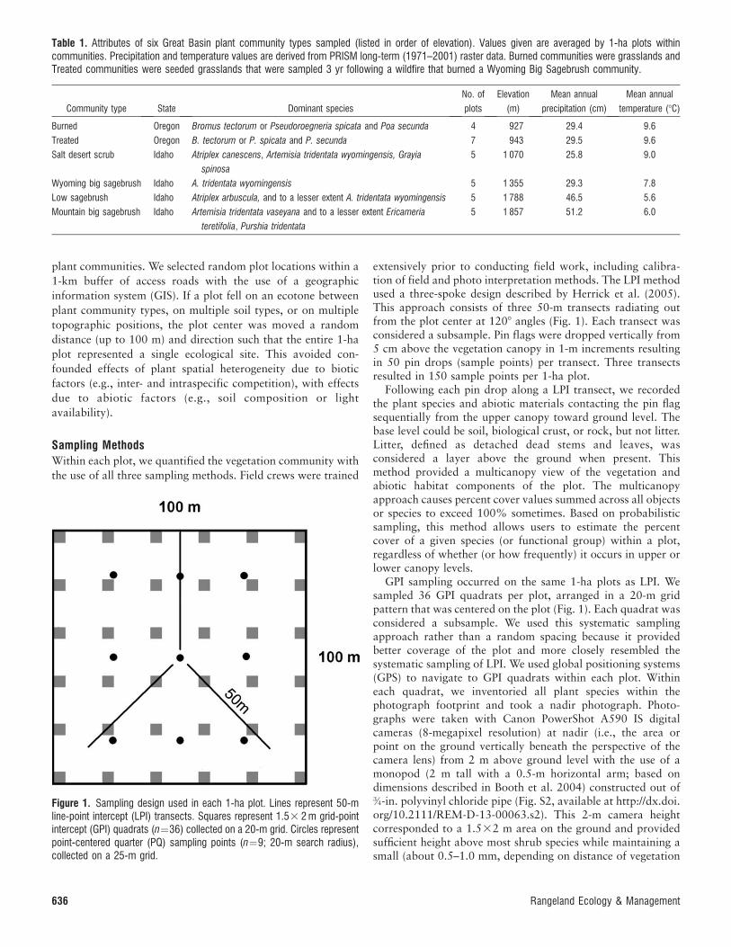
extensively prior to conducting field work, including calibra-tion of field and photo interpretation methods. The LPI methodused a three-spoke design described by Herrick et al. (2005).This approach consists of three 50-m transects radiating outfrom the plot center at 1208 angles (Fig. 1). Each transect wasconsidered a subsample. Pin flags were dropped vertically from5 cm above the vegetation canopy in 1-m increments resultingin 50 pin drops (sample points) per transect. Three transectsresulted in 150 sample points per 1-ha plot.

Following each pin drop along a LPI transect, we recordedthe plant species and abiotic materials contacting the pin flagsequentially from the upper canopy toward ground level. Thebase level could be soil, biological crust, or rock, but not litter.Litter, defined as detached dead stems and leaves, wasconsidered a layer above the ground when present. Thismethod provided a multicanopy view of the vegetation andabiotic habitat components of the plot. The multicanopyapproach causes percent cover values summed across all objectsor species to exceed 100% sometimes. Based on probabilisticsampling, this method allows users to estimate the percentcover of a given species (or functional group) within a plot,regardless of whether (or how frequently) it occurs in upper orlower canopy levels.

GPI sampling occurred on the same 1-ha plots as LPI. Wesampled 36 GPI quadrats per plot, arranged in a 20-m gridpattern that was centered on the plot (Fig. 1). Each quadrat wasconsidered a subsample. We used this systematic samplingapproach rather than a random spacing because it providedbetter coverage of the plot and more closely resembled thesystematic sampling of LPI. We used global positioning systems(GPS) to navigate to GPI quadrats within each plot. Withineach quadrat, we inventoried all plant species within thephotograph footprint and took a nadir photograph. Photo-graphs were taken with Canon PowerShot A590 IS digitalcameras (8-megapixel resolution) at nadir (i.e., the area orpoint on the ground vertically beneath the perspective of thecamera lens) from 2 m above ground level with the use of amonopod (2 m tall with a 0.5-m horizontal arm; based ondimensions described in Booth et al. 2004) constructed out ofł-in. polyvinyl chloride pipe (Fig. S2, available at http://dx.doi.org/10.2111/REM-D-13-00063.s2). This 2-m camera heightcorresponded to a 1.532 m area on the ground and providedsufficient height above most shrub species while maintaining asmall (about 0.5–1.0 mm, depending on distance of vegetation

Table 1. Attributes of six Great Basin plant community types sampled (listed in order of elevation). Values given are averaged by 1-ha plots withincommunities. Precipitation and temperature values are derived from PRISM long-term (1971–2001) raster data. Burned communities were grasslands andTreated communities were seeded grasslands that were sampled 3 yr following a wildfire that burned a Wyoming Big Sagebrush community.

Community type State Dominant species

No. of

plots

Elevation

(m)

Mean annual

precipitation (cm)

Mean annual

temperature (8C)

Burned Oregon Bromus tectorum or Pseudoroegneria spicata and Poa secunda 4 927 29.4 9.6

Treated Oregon B. tectorum or P. spicata and P. secunda 7 943 29.5 9.6

Salt desert scrub Idaho Atriplex canescens, Artemisia tridentata wyomingensis, Grayia

spinosa

5 1 070 25.8 9.0

Wyoming big sagebrush Idaho A. tridentata wyomingensis 5 1 355 29.3 7.8

Low sagebrush Idaho Atriplex arbuscula, and to a lesser extent A. tridentata wyomingensis 5 1 788 46.5 5.6

Mountain big sagebrush Idaho Artemisia tridentata vaseyana and to a lesser extent Ericameria

teretifolia, Purshia tridentata

5 1 857 51.2 6.0

Figure 1. Sampling design used in each 1-ha plot. Lines represent 50-mline-point intercept (LPI) transects. Squares represent 1.53 2 m grid-pointintercept (GPI) quadrats (n¼36) collected on a 20-m grid. Circles representpoint-centered quarter (PQ) sampling points (n¼9; 20-m search radius),collected on a 25-m grid.

636 Rangeland Ecology & Management

to camera lens) ground sample distance (GSD; the actual lineardistance represented by each pixel composing an image).

We used SamplePoint 1.43 software (Booth et al. 2006a) tomeasure the cover of species and functional groups at 100computer-selected grid points on each image. The pixel GSD ofapproximately 0.5–1.0 mm (a single grid point) was approx-imately half the diameter of the wire pin flags used for LPI. Wemeasured cover as the percentage of grid points that ‘‘hit’’ aspecies or abiotic habitat component, which collectivelysummed to 100% across each quadrat (i.e., photograph). Wereferred to the species lists collected in the field at each quadratonly if we were uncertain about a species’ identification in theimage.

Aboveground photography provides a bird’s-eye view of theplot. Therefore, GPI measures cover as the percentage of pointswithin the photograph extent (footprint) where a species orfunctional group occurs as the uppermost object (i.e., visiblefrom above). However, it is important to note that photogra-phy-based GPI does not provide a single-canopy view, at leastat the quadrat level. Where plant canopies were absent (e.g.,canopy gaps), we could detect litter, biological soil crust, or soilon the ground surface. Therefore, within each quadrat, we wereable to measure cover of understory species and litter, and to alesser extent, soil exposure.

We used the PQ method to quantify the percent cover ofrelatively rare plants, such as mature native bunchgrasses andshrubs in burned areas and scattered juniper trees. We sampledbunchgrass, shrub, and tree functional groups at nine PQsampling points in each 1-ha plot (Fig. 1). Each PQ point wasconsidered a subsample of the 1-ha plot. Sampling points wereestablished with the use of a 25-m grid centered on the plotcenter. At each sample point and for a given target functionalgroup (i.e., bunchgrass, shrub, or tree), we measured the lineardistance to the centroid of the nearest individual in fourquadrants (NW, NE, SE, and SW) within a 20-m search radius.We then repeated the process for the two other functionalgroups. Thus, we measured up to 36 bunchgrass, 36 shrub, and36 tree individuals per plot if all nine PQ sampling points andtheir four associated quadrants had qualifying individualswithin 20 m. For each qualifying plant, we also measured itsdiameter (i.e., canopy intercept). Canopy intercept was equal tothe distance between the first point of vertical intercept and thelast point of vertical intercept through the canopy of anindividual plant. To be counted, the canopy intercept wasrequired to be �15 cm for a bunchgrass and �10 cm for ashrub or tree. If these conditions were not met, the next nearestplant (within the 20-m search radius) meeting the conditionswas measured. These size restrictions were imposed to reduceobserver bias for large plants and to exclude Poa species, whichwere generally common enough to be measured using the othermethods. If no qualifying plants were present within 20 m, werecorded a distance of 20 m and a canopy intercept of 0 cm.

Data Analysis

Percent Cover. With the use of LPI and GPI data, wegenerated percent cover estimates for each 1-ha plot at twotaxonomic resolutions: species and functional groups. Weassigned each species or abiotic habitat component to 1 of 10functional groups on the basis of morphology and life history:

Tree, Shrub, Perennial Grass, Exotic Annual Grass (hereafterAnnual Grass), Exotic Forb, Native Forb, Litter (detachedplant matter , 5-mm diameter), Coarse Woody Debris (�5-mm diameter), Soil, and Rock (�5-mm minimum diameter).

With the use of LPI data, we quantified percent cover as thenumber of pin-drop locations (out of 50 possible for eachtransect line) where a given plant species, or functional group,contacted the pin flag. We then averaged the cover measure-ments for the three transects within each 1-ha plot. We repeatedthis process for each plot with the use of only the uppermostspecies or functional group contacting the pin flag on each pindrop (LPI top canopy hit only). This allowed us to examine therelationship between cover estimates generated by LPI and GPI,because GPI is a view-from-above technique. We also were ableto determine how much information about lower canopies waslost as a result of nadir sampling techniques.

To generate percent cover estimates for each 1-ha plot withthe use of GPI data, we first divided the number of grid pointsrepresenting a given species or functional group in an image bythe total number of grid points classified per image (usually100). We then averaged the percent cover values for eachspecies and functional group across the 36 quadrats (photo-graphs) within each 1-ha plot.

With the use of PQ data, we estimated density and percentcanopy cover of Tree, Shrub, and Perennial Grass functionalgroups by averaging nine PQ sample points across each 1-haplot. The density (number of individuals �m�2) of a givenfunctional group was calculated as: 1/(x̄d1, d2, d3, d4)2 whered¼the point-to-plant distance (m) for the closest qualifyingplant in each of the four quadrants. This density measurementwas used along with canopy intercept data to calculate percentcover at each PQ sample point as: (x̄a1, a2, a3,a4) � (density) � (100), where a¼area of plant’s canopy; calcu-lated as: 1/2p(canopy intercept in meters)2.

We performed paired regression analyses of each functionalgroup and method. This allowed us to examine percent covervalues generated along vegetation and successional gradients,and among plant communities, with the use of the threesampling methods. Each regression had a sample size of 31plots from six community types. We assessed the correspon-dence of cover values from different sampling techniques byexamining the r-squared value (r2) and slope term (b) from eachregression analysis. When within-plot cover values from eachpaired method were strongly associated, r2 approached 1.When there was high within-plot agreement on cover values, a1:1 relationship existed and b approached 1 (this also assumesthat the intercept approached zero, which it did). Thus, theoverall correspondence of percent cover values from differentsampling techniques was greatest when both r2 and b¼1. Notethat within-plot cover estimates could be strongly associated(high r2) without providing similar numerical values (b muchgreater or less than 1).

Community Composition. We examined the performance of LPIand GPI methods in quantifying plant community compositionwith the use of nonmetric multidimensional scaling ordination(NMS; PC-ORD 5.10 software; McCune and Mefford 2006).For this analysis, we treated the GPI data and the LPI datacollected on a given plot as separate sample units. Thus, thenumber of sample units (i.e., plots) in the analysis was 62 (i.e.,

66(6) November 2013 637

31 pairs of plots), where each pair represented one physicallocation where vegetation was quantified in two different ways.We generated a NMS ordination biplot with the use of percentcover of functional groups for each plot pair. Plots nearer eachother in ordination space had more similar plant communities.Consequently, if LPI and GPI represented the vegetation of agiven plot identically, the two ordination biplot points for thatplot (i.e., one for GPI and one for LPI) would overlap inordination space. NMS analyses were run with the use ofmethods described in Arkle et al. (2010).

Within-Plot Subsampling. We assessed subsampling adequacyto evaluate how well three transects, 36 GPI quadrats, and ninePQ sampling points characterized vegetation in 1-ha plots. Foreach sampling method, functional group, and plot, we plottedthe relative standard error (RSE¼SE/mean) of percent coverestimates against the mean percent cover estimate for the plot.Logarithmic functions were fitted to these data. We expectedthat RSE should decrease as the estimate of percent coverincreases for a particular functional group. Based on thisexpectation, the appropriate number of within-plot subsamplesshould not be constant, but should instead depend on the totalpercent cover of the functional group and on its distributionwithin the plot. RSE values greater than 20% are generallyconsidered high for ecological studies (McCune and Grace2002) and indicate high spatial heterogeneity or inadequatewithin-plot subsampling. Therefore, with the use of the fullnumber of within-plot subsamples for each sampling method(n¼three LPI transects, 36 GPI quadrats, and nine PQ samplesper plot), we determined percent cover values of differentfunctional groups where RSE was �20%.

We also examined within-plot subsampling adequacy at thecommunity level. We evaluated only the GPI method with theuse of this approach because the LPI method had too fewwithin-plot subsamples and the PQ method only generatedpercent cover estimates for 3 of the 10 possible functionalgroups within each plot. With the use of PC-ORD 5.10

software (McCune and Medford 2006), distance-area (ordistance-effort) curves were generated separately for each plotto determine the minimum number of GPI quadrats required torepresent the entire vegetation community of the plot. Thismethod is analogous to the more familiar species-area (orspecies-effort) curve, except that it incorporates information onboth species presence and abundance in each subsample(quadrat). For each plot, we took 500 bootstrap resamples(with replacement) of GPI quadrats at each possible number ofsubsamples (i.e., 1–35 quadrats). We then calculated theSorenson distance between the vegetation community asrepresented by all 36 GPI quadrats and the vegetationcommunity as represented by fewer (i.e., 1–35) of the 36quadrats. When the average distance between a subset of GPIquadrats and the entire population of 36 GPI quadrats is small(e.g., , 10%, McCune and Grace 2002), the lower number(subset) of quadrats is effectively representing the vegetationcommunity in the plot, regardless of which particular quadratsare included. For each plot, we determined the number of GPIquadrats, which resulted in an average Sorenson distance of, 10% from the entire population of 36 GPI quadrats. Thisnumber of GPI quadrats per plot was averaged by communitytype. We repeated these analyses first with the use of species-level and then functional group-level cover data with andwithout abiotic habitat components (e.g., litter, soil) becausewe suspected that the amount of within-plot replicationrequired to represent vegetation communities might dependon the taxonomic resolution of the plant community and on theinclusion of common abiotic components (e.g., litter or soil).

Effort Requirements. Effort requirements for all three methodswere evaluated on the basis of time required for a crew, trainedin sampling methods and vegetation identification, to set upand complete sampling (including photographic analysis timefor GPI) for each plot. We calculated the number of person-hours used on each plot per subsample and per measurementpoint (pin drop for LPI and pixel for GPI). Values wereaveraged by community type and across all plots.

For the LPI method, we examined the amount of informationgained through the additional sampling effort of recordingunderstory species. We determined the probability of lowercanopy (i.e., understory) plants contacting the pin flag in eachplot and averaged these values across community types. Thisanalysis also gives an indication of the amount of plant-coverinformation lost through nadir sampling approaches likephotography-based GPI.

RESULTS

Quantifying Percent Cover

Point-Intercept Methods. We generated percent cover estimatesin 1-ha plots for 52 plant species with the use of the LPIsampling method and 64 species with the use of the GPImethod across all plant communities. We found that percentcover values obtained with the use of LPI and GPI weresignificantly correlated for most functional groups at the plotlevel (Table 2). There was no significant effect of communitytype on the relationship between percent cover values derivedfrom LPI and GPI. Therefore, in subsequent regression

Table 2. r2 and slope coefficient values for the relationships betweenpercent cover of different functional groups as measured with the use ofgrid-point intercept (GPI) and line-point intercept (LPI) in 31 1-ha plots fromsix community types. Values are shown for two scenarios, one where LPIcover is calculated with the use of all canopy data (all hits) and the otherwhere LPI cover is calculated with the use of only the uppermost canopydata (top hit only). The percent change in slope (%Db) indicates themagnitude of change in b when LPI cover is calculated two different ways.No trees were detected with the use of the LPI sampling technique.

Functional group

GPI vs. LPI all hits GPI vs. LPI top hit only

%Dbr2 b r2 b

Rock 0.85 0.86 0.68 1.01 15

Soil 0.01 �0.05 0.88 0.87 92

Litter 0.01 0.02 0.01 0.04 2

Coarse woody debris 0.26 0.17 0.12 0.20 3

Annual grass 0.94 0.91 0.95 1.01 10

Perennial grass 0.90 0.51 0.94 0.83 32

Exotic forb 0.95 0.50 0.96 0.70 20

Native forb 0.90 0.52 0.81 0.70 18

Shrub 0.92 0.88 0.92 0.91 3

638 Rangeland Ecology & Management

Figure 2. Percent cover of six functional groups measured in 1-ha plots (n¼31) with the use of grid-point intercept (GPI) and line-point intercept (LPI)methods. Plots are symbolized by community type (n¼6). The solid line was fitted with the use of regression, and the dashed line represents a 1:1relationship in cover values between methods (b¼1). Several functional groups are not shown, but are listed in Table 2. See text for plant functional groupand vegetation community type descriptions.

66(6) November 2013 639

analyses, community type was not included as a cofactor. Shruband Annual Grass functional group cover estimated from LPI

were both strongly correlated with estimates from GPI, andvalues were nearly 1:1 between methods (Table 2). Percentcover values for Perennial Grass, Exotic Forb, and Native Forb

functional groups also were strongly correlated, but covervalues generated from GPI were substantially lower than those

generated with the use of LPI (Table 2) even when thesefunctional groups were the uppermost canopy present on the

plot (e.g., Perennial Grass on Burned or on Treated plots; Fig.2). Litter and Soil cover values generated with the use of the

two methods were uncorrelated. GPI-derived Litter coverestimates showed little variability among plots (0–10% littercover for all plots; Fig. 2) and LPI-derived Soil cover estimatesshowed little variability among plots (80–100% soil cover forall plots). Trees were not detected with the use of LPI (evenwhen pin flags were projected upwards), but seedlings orbranches that were lower than 2 m were determined to

comprise up to 2.5% cover with GPI methods.

The correspondence between cover estimated from LPI andGPI methods improved when we used only the uppermostobject contacting each pin flag (i.e., top hit) for LPI estimates

Figure 3. Percent cover of Shrub and Perennial Grass (excluding Poa secunda) functional groups measured in 1-ha plots (n¼31) with the use of point-centered quarter (PQ) and line-point intercept (LPI) methods (left column), and PQ and grid-point intercept (GPI) methods (right column). Plots aresymbolized by community type (n¼6). The solid line was fitted with the use of regression and the dashed line represents a 1:1 relationship in cover valuesbetween methods (b¼1). Tree functional group is not shown. See text for plant functional group and vegetation community type descriptions.

640 Rangeland Ecology & Management

(Table 2). This improvement was observed primarily for lowercanopy species.

PQ Method. PQ cover results were comparable to those ofLPI and GPI across cover gradients and among plantcommunities. We detected nine perennial bunchgrass, 14shrub, and two tree species across all plots with the use of thePQ method. In the same plots, we detected eight perennialbunchgrass, 12 shrub, and no tree species using the LPImethod. Percent cover values obtained using PQ and LPI werestrongly correlated (Fig. 3). For Shrubs, the b value betweenLPI and PQ methods was nearly 1 (Table 3). For Perennial

Grass, however, the PQ estimate of cover was approximately

half that of the LPI estimate (b¼0.49; Table 3). Lower cover

derived from the PQ method was likely influenced by the

methodological restriction that only bunchgrasses with

canopy intercept �15 cm were included in PQ cover

measurements. In contrast, we included bunchgrasses of any

size when measuring Perennial Grass cover using the LPI

method. The 1:1 correspondence between cover estimates

generated from these two sampling methods improved (bcloser to 1) when only LPI top-hit data were used to determine

percent cover values (Table 3).

We detected the same bunchgrass, shrub, and tree species

with the use of GPI as were detected with the use of PQ.

Percent cover values obtained with the use of PQ and GPI

were strongly correlated for Shrub and Perennial Grass

(excluding Poa secunda cover) functional groups (Table 3

and Fig. 3) and b values were close to 1. Tree functional group

cover was correlated between the two techniques (r2¼0.65);

however, the observed range of tree cover was limited to only

0–3%. There was high variability in tree-cover estimates

among GPI quadrats at plots where trees were detected

(SE¼mean cover value in all seven plots). Standard error of

tree cover estimates was less when PQ was used (SE , 100%

of mean cover value in six of seven plots where trees were

detected with the use of PQ).

Table 3. r2 and slope coefficient values for the relationships betweenpercent cover as measured with the use of the point-centered quartermethod (PQ) and line-point intercept (LPI) or PQ and grid-point intercept(GPI). Values are shown for analyses where LPI all-hit and top-hit only datawere used. No trees were detected with the use of the LPI samplingtechnique.

Functional group

PQ vs. LPI all hits PQ vs. LPI top hit only PQ vs. GPI

r2 b r2 b r2 b

Perennial grass 0.81 0.49 0.79 0.80 0.9 0.85

Shrub 0.90 0.95 0.90 0.98 0.95 1.08

Tree – – – – 0.65 0.43

Figure 4. Nonmetric multidimensional scaling (NMS) ordination biplot of cover data for seven plant functional groups measured on the same 1-ha plotswith the use of line-point intercept (LPI) (darker symbols) and grid-point intercept (GPI) (lighter symbols) sampling methods across six vegetationcommunity types. See text for plant functional group and vegetation community type descriptions.

66(6) November 2013 641

Community Composition

NMS ordination of cover data for seven plant functional

groups measured with LPI and GPI on the same 1-ha plots

produced a two-axis solution (stress¼12.15, P¼0.003) repre-

senting 92% of the variance in the original data. Axis 1

represented 58% of the variance in the original data and

described a gradient of dominance from Annual Grass

(increasingly positive Axis 1 values) to Native Forb, Shrub,

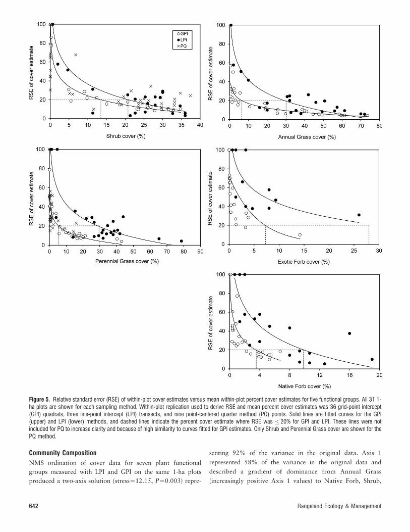
Figure 5. Relative standard error (RSE) of within-plot cover estimates versus mean within-plot percent cover estimates for five functional groups. All 31 1-ha plots are shown for each sampling method. Within-plot replication used to derive RSE and mean percent cover estimates was 36 grid-point intercept(GPI) quadrats, three line-point intercept (LPI) transects, and nine point-centered quarter method (PQ) points. Solid lines are fitted curves for the GPI(upper) and LPI (lower) methods, and dashed lines indicate the percent cover estimate where RSE was � 20% for GPI and LPI. These lines were notincluded for PQ to increase clarity and because of high similarity to curves fitted for GPI estimates. Only Shrub and Perennial Grass cover are shown for thePQ method.

642 Rangeland Ecology & Management

and Tree cover (increasingly negative Axis 1 values; Fig. 4).Axis 2 represented 34% of variance and was positivelyassociated with cover of Perennial Grass and Poa secundafunctional groups. Plot pairs, measured with the use of the twosampling methods, tended to separate along Axis 2. For mostplots, community composition tended to be more associatedwith the Perennial Grass (including Poa secunda) functionalgroup when measured with the use of LPI than when thecommunity composition in the same plot was quantified withthe use of GPI. In general, however, the two sampling methodsproduced similar representations of community composition.

Within-Plot Subsampling

Functional Group Level. The number of subsamples (i.e., LPItransects, GPI quadrats, PQ points) required to meet the RSEcriterion (i.e., RSE , 20%) depended on functional groupcover within each 1-ha plot (Fig. 5). The RSE of the percentcover estimate tended to be low when the percent cover of aparticular functional group was high within a plot. As the coverof the functional group decreased within plots, RSE valuesincreased toward 100%. Community type did not have asignificant influence on the relationship between RSE and meancover estimates, and was therefore not included as cofactor inanalyses. Logistic functions fit the observed data well, with r2

values between 0.65 and 0.98 (Fig. 5).

We found that the mean percent cover of shrubs had to begreater than 21% for three LPI transects (number ofsubsamples per 1-ha plot) to have RSE values below the 20%threshold (Fig. 5). When LPI Shrub cover estimates were lessthan 21%, the standard error was very high relative to themean; we observed only five plots where shrub cover wasgreater than zero, but less than 21%. In contrast to the LPImethod, 36 GPI quadrats per 1-ha plot were insufficient whenShrub cover was �13%. When GPI Shrub cover estimateswere less than 13%, the standard error was fairly low relativeto the mean (RSE , 30% when Shrub cover was between 5%

and 10%). We detected shrubs in 29 of 31 plots with the use thePQ method and thus only 2 PQ plots had values of zero inFigure 5 (8 plots had nonzero values that appear close to the yaxis). Relative to the other methods, PQ estimates of Shrubcover had lower RSE values at the low end of the range of covervalues. PQ did not perform as well as the other methods whenShrub cover was . 20%.

A similar pattern was observed for Perennial Grass, AnnualGrass, Exotic Forb, and Native Forb cover. Thirty-six GPIquadrats per 1-ha plot were sufficient for RSE to be less thanthe 20% threshold when percent cover estimates were in the 4–7% range (depending on the functional group). Percent coverestimates from LPI had to be two–three times greater than GPI-derived estimates for RSE values , 20% (Fig. 5). For example,three LPI transects were insufficient to generate RSE values, 20% when Annual Grass or Perennial Grass cover were� 30%. When Perennial Grass cover was estimated with theuse of the PQ method, RSE values were comparable to thosegenerated by GPI and lower than values from LPI. RSE valuesfrom PQ were lower than GPI values when Perennial Grasscover was , 5%, further demonstrating the utility of PQ whentarget species or functional groups are rare (Fig. 5).

Community Level. Distance-area curves generated for eachplot (for example, Fig. S3; available at http://dx.doi.org/10.2111/REM-D-13-00063.s3) indicate that the minimum numberof GPI quadrats required to represent the composition andabundance of the vegetation in each plot varies withcommunity type and with the desired taxonomic resolution(Table 4). The mean number of GPI quadrats needed torepresent the community with functional groups (with bothbiotic and abiotic variables) was 5.8, whereas 11.7 quadratswere required to represent the community with species(without abiotic habitat cover included). In general, plots inhigher elevation and more complex communities required moresubsamples to meet the 10% reference level (Table 4).

Use of species-level percent cover data required two–fivemore subsamples than were required when functional group-level cover data were used. Including percent cover data onabiotic habitat components decreased the number of samplesrequired by two–four GPI quadrats per plot (Table 4).

Effort RequirementsRegardless of the community type, the average amount of fieldtime required for two-person teams to sample a single 1-ha plotwas 1 h and 25 min for LPI (three 50-m transects), 1 h and 15min for GPI (36 quadrats), and 1 h and 20 min for PQ (9points). These estimates included time required for setup andtime required for collecting ancillary data on plant height,species checklists, and plot information. After factoring inadditional time requirements for photographic analysis (GPIrequired 5 min per image [3 s per pixel] on average) andadditional personnel requirements (LPI is more efficient withtwo people—one data reader and one recorder—but fieldtechnicians can work independently when using the other twomethods), we found that 6.7 GPI quadrats can be acquired forevery LPI transect (Fig. S4, available at http://dx.doi.org/10.2111/REM-D-13-00063.s4). Therefore, 20–25 GPI quadratsper 1-ha plot represented equal effort (in terms of person-hours) to collecting the standard three LPI transect lines per 1-

Table 4. With the 10% Sorenson distance used as a cutoff, the averagenumber of within-plot grid-point intercept (GPI) quadrat subsamplesnecessary to represent the vegetation community (as represented by 36quadrats) in 1-ha plots is shown. Values shown are the mean number ofGPI quadrats from all plots (n¼4–7) per community type. Four separateanalyses were run for each plot with the use of functional group-level andspecies-level cover data and including or excluding percent cover of abiotichabitat components (Litter, Coarse Woody Debris, Soil, Rock). Values inparentheses exclude one partly burned plot.

Community type

Functional groups Species

Biotic

only

Biotic and

abiotic

Species

only

Species and

abiotic

Burned 6.5 5.5 7 5.5

Treated 8

(6.7)

5.4

(5.2)

9.3

(7.5)

6.1

(5.8)

Salt desert scrub 7.4 4.4 13 6.2

Wyoming big sagebrush 7.2 6.4 10.2 8.2

Low sagebrush 9.4 6.4 14 8.8

Mountain big sagebrush 7.8 6.2 14.4 10

66(6) November 2013 643

ha plot. Approximately 10 PQ points per 1-ha plot equals thenumber of person-hours required to complete three LPItransects.

Based on a total of 2 400 LPI pin drops, the probability ofcontacting one plant species was 0.52–0.66, depending oncommunity type (Fig. 6). Across all community types only 60%of pin drops contacted any plants; the other 40% contactedonly abiotic functional groups. The probability of a pin flagcontacting more than one species dropped sharply, with lessthan 1% of pins contacting three different species (Fig. 6). Theprobability of contacting one or two plant species was higher incommunity types with increasing elevation and precipitation,except for the Burned and Treated community types, which hadthe highest probabilities of observing one plant, but interme-diate probabilities of detecting two plant species.

For most biotic functional groups, there was high agreementin percent cover estimates derived from LPI ‘‘top-hit only’’ dataand LPI ‘‘all hit’’ data (Table 5). The relationship was strongestfor Shrub and Annual Grass functional groups. Abioticfunctional groups were either not correlated, or had relativelylow r2 and b values. This was the same trend as was observed inthe relationship between GPI and LPI top-hit only coverestimates (Table 2). Using LPI top-hit only data reduced speciesrichness by an average of 0.39 species per transect line, with amaximum reduction of two species in any transect. However, atthe plot level we found no net loss of species richness in any ofthe 31 plots.

DISCUSSION

All three methods performed well in characterizing shrublandand grassland vegetation in these northern Great Basin plantcommunities. Some aspects of their performance were influ-enced by environmental or vegetation conditions.

Cover Estimates Across Vegetation GradientsThe comparability or interchangeability of cover estimatesderived from different methods is important for our purposesbecause it is a means of assessing relative accuracy (i.e.,closeness to ‘‘truth’’) when true cover values within plots areunknown. From a broader perspective, comparability amongmethods is important for researchers needing to use or convertdata from different sources, or for compiling data to createmeaningful regional assessments (Godinez-Alvarez et al. 2009).

Regardless of community type or vegetation cover, the LPIand GPI methods produced estimates of cover that were highlycorrelated for most biotic functional groups, a findingcongruent with a similar study that investigated five plantcommunities in the Chihuahuan Desert (Godinez-Alvarez et al.2009). In particular, the two methods produced nearlyequivalent (b ’ 1) shrub cover estimates, which is encouraginggiven the recent emphasis on monitoring shrub cover forwildlife such as greater sage grouse (Centrocercus urophasia-nus). Also, it demonstrates that within the community typesexamined, photography-based GPI does not overestimate coverrelative to LPI when tall (e.g., sagebrush or bitterbrush) plantsare prevalent because of issues associated with parallax. Coverestimates for another important functional group, exoticannual grasses (mostly cheatgrass, Bromus tectorum), werealso comparable between LPI and GPI.

The GPI method tended to underestimate bunchgrasses andforbs relative to LPI, which is partly a methodological artifact;LPI provides multicanopy data, whereas GPI provides infor-mation on only the uppermost plant at any given point. This issupported by our finding that top-hit data from LPI resulted inincreased agreement in cover estimates between LPI and GPI.This is not the only explanation, though, as LPI still tended tooverestimate bunchgrass, native forb, and exotic forb coverrelative to GPI, even in Burned and Treated community typeswhere these plants were always the uppermost canopy of plots.

Figure 6. For each community type, the average probability of a line-pointintercept (LPI) pin contacting one or more plant species. Estimates werebased on 150 pin drops per 1-ha plot and probabilities from each plot wereaveraged by community type (n¼4–7 plots in six community types). Thusestimates were derived from 600, 750, and 1 050 total pin drops incommunities where four, five, or seven plots were sampled, respectively.Error bars were omitted for clarity, but SE values for the ‘‘One plant’’column ranged from a low of 60.06 for Salt Desert Scrub to a high of60.022 for Mountain Big Sagebrush. See text for plant functional groupand vegetation community type descriptions.

Table 5. r2-squared and slope coefficient values for the relationshipsbetween percent cover as measured with the use of line-point intercept(LPI) top-hit and LPI all-hit data. No trees were detected with the use of theLPI sampling technique.

Functional group r2 b

Rock 0.95 0.63

Soil 0.01 0.06

Litter 0.17 0.14

Coarse woody debris 0.68 0.46

Annual grass 0.98 0.89

Perennial grass 0.94 0.78

Exotic forb 0.98 0.71

Native forb 0.96 0.68

Shrub 0.99 0.96

644 Rangeland Ecology & Management

We suspect there may also be some observer bias associatedwith LPI because field personnel decide whether a plant iscontacting a pin flag when it is close to the pin, an issue that iscomplicated by the movement of flexible plants in even lightwinds (Cagney et al. 2011). Further, the pixel size in ourphotography-based GPI was about half the diameter of the pinused by field crews, depending on the distance of the plant tothe lens. Finally, even slight deviations from vertical whenholding a pin flag greatly increase the plant–pin contact area.Collectively, these factors may increase the number of LPIpoints contacting vegetation relative to photography-based GPIpoints (Booth et al. 2005). With 50 sampling points per LPItransect, each additional sampling point where a given speciescontacts a pin flag results in a 2% increase in the cover estimatefor that species.

We found that across community types, PQ and GPI resultedin similar estimates of shrub and bunchgrass (excluding Poasecunda) cover. This was surprising given that there aresubstantial differences between these two techniques, includingan area-based versus plotless approach, and a size requirementfor PQ where shrubs and bunchgrasses smaller than 10–15 cmdiameter were excluded. However, excluding Poa secunda fromGPI cover estimates for this particular analysis meant thatpredominantly larger individuals (e.g., . 15 cm diameter) wereincluded in GPI cover estimates and it was these largerindividuals that were targeted using the PQ method. Forshrubs, individuals , 10 cm in diameter contributed little to thetotal plot area covered by shrubs. Consequently, excludingsmaller individuals had little effect on PQ estimates.

PQ and LPI cover estimates were also well correlated andnearly 1:1 for shrubs. However, for bunchgrasses, PQunderestimated cover relative to LPI. Although, as with GPI,correspondence improved when LPI top-hit only data wereused. However, LPI still produced slightly higher coverestimates than PQ even after applying this correction (possiblyfor reasons similar to those discussed above).

Precision of Cover Estimates Across Vegetation GradientsSuccessfully quantifying vegetation and detecting change inheterogeneous shrublands depends on reasonably precisemeasurements of cover (e.g., Havstad and Herrick 2003). Wefound that regardless of community type, the precision of coverestimates across 1-ha plots was highly dependent on theabundance (i.e., cover) of the species or functional group beingmeasured. When cover values within plots were low, precisionwas low and methodological approach (e.g., LPI, GPI, PQ),number of subsamples (i.e., number of line transects, quadrats,PQ points), and vegetation characteristics (i.e., communitytype, within-plot patchiness) had comparatively small influ-ences on precision. Precise estimates of cover are critical fordetecting small changes in vegetation cover through time andproviding a level of confidence on cover estimates. Forexample, this precision may be important for managementdecisions regarding wildlife and range health.

The GPI method produced fairly precise estimates of coveracross the range of cover values and vegetation communities.Photography-based GPI has been shown to produce preciseestimates of cover (Booth et al. 2006a; Seefeldt and Booth2006), although our results show that this precision is

dependent on the cover of target species or functional groups.Sample sizes of six–nine GPI quadrats per hectare adequatelycharacterized these vegetation communities, but when covervalues were below 5–10%, even 36 GPI quadrats per hectarewas insufficient to estimate cover precisely for most functionalgroups. Inouye (2002) found that species with average coverless than 5% required more than 50 GPI quadrats (0.531.0 mframes) to achieve adequate precision in a 1.4-ha study plotthat was dominated by Wyoming big sagebrush.

Depending on the functional group, LPI cover estimates hadto exceed 10–30% cover and GPI cover estimates had to exceed5–13% cover to be estimated precisely. LPI measurements ofcover are fairly unbiased relative to other estimators (Elzinga etal. 2001), except when target objects are rare (Stohlgren et al.1998). Methodological tests have found that it can take about2 000 points to estimate the cover of species with , 8% coverwithin 10% of the mean with 95% confidence (Walker 1970).Our 150 LPI points per plot is only 7.5% of this recommendedcriteria. Our photography-based GPI resulted in 3 600 pointsper 1-ha plot (100 points within each of 36 3-m2 quadrats), anamount that could still be considered insufficient at low covervalues. Clearly, when target species or functional groups arerare, or as vegetation heterogeneity increases, some adaptationof methods may be necessary, such as increasing the number ofpoints per subsample (i.e., more transect lines or quadrats) ornumber of subsamples per plot (Fisser and VanDyne 1966;Floyd and Anderson 1987; Brady et al. 1995; Inouye 2002). Atcover values less than 10%, the PQ estimates producedcomparatively low relative standard error values, indicatingthat this method is well suited for measuring cover of sparseplants and could be used to supplement other methods whencover values of target species or functional groups are low.

At the community level (i.e., all functional groups consideredtogether), we found that the average number of within-plot GPIquadrats necessary to represent plot conditions depended oncommunity type and on whether species or functional groupswere analyzed. When biotic and abiotic functional groups wereanalyzed together to represent plot conditions, approximatelysix GPI quadrats were needed regardless of community type.However, when species were analyzed without abiotic habitatcomponents, 7–14 GPI quadrats were needed, with this valuedepending more strongly on community type. Low Sagebrushand Mountain Big Sagebrush communities, which occur athigher elevations, required more subsamples than Wyoming BigSagebrush or Salt Desert Scrub communities. Grasslands (i.e.,Burned community type) and seeded areas formed by recentwildfire and restoration activities (i.e., Treated communitytype) had simple vegetation composition and structure andrequired less subsampling and sample replication than the otherhabitat types.

Representing Community CompositionAcross a broad range of successional and invasive plantdominance conditions, GPI and LPI sampling methods pro-duced very similar representations of community composition.For example, in three of five Salt Desert Scrub plots,community composition was nearly indistinguishable betweenthe two methods. Both sampling methods also indicated thatMountain Big Sagebrush and Low Sagebrush plant communi-

66(6) November 2013 645

ties were similar to one another at the functional group level,although GPI yielded slightly better separation of these twocommunities. PQ was not used for measuring communitycomposition.

In preliminary analyses, we found that community-levelordinations with abiotic functional groups included resulted inpoor agreement between the two methods. This was because93% of LPI points contacted Soil and 59% contacted Litter,whereas these functional groups were far less common in theGPI data (38% and 5% cover on average, respectively). Thus,differences among biotic functional groups were trivialized bydifferences among abiotic functional groups. Use of LPI top-hitonly data, instead of multiple-canopy data, improved agree-ment between the two methods.

Point-based methods, such as LPI and GPI, have beenconsidered inadequate to monitor biological diversity becausethey often fail to detect rare species (Stohlgren et al. 1998).Although we found similar species assemblages with the use ofthe three methods, we did not assess the effectiveness of thesemethods for detecting rare species. This is usually betteraccomplished through visual surveys. However, we found thatPQ was adept at detecting and providing percent coverestimates for sparse plants, potentially making this methoduseful for research or monitoring programs involving low-abundance target species. Similarly, an added feature of the GPImethod is the ability to search each quadrat area for speciesoccurrence visually, which can be summed across the subsam-ples in a given plot to provide frequency estimates when coveris low within quadrats.

Efficiency of Vegetation SamplingIn agreement with past studies, the GPI method produced arelatively high number of subsamples per unit effort (e.g., Brunand Box 1963; Booth et al. 2005). Booth et al. (2005) foundhigh efficiency even when image processing time was includedin calculations. This efficiency may be particularly importantwhen vegetation is spatially heterogeneous because largersample sizes (i.e., more plots and within-plot subsamples) arerequired for adequate precision of cover and species richnessestimates. After adjusting for photograph analysis time, wefound that 20–25 GPI quadrats per hectare represented equaleffort, in terms of person-hours, to collecting data in 1-mintervals on three 50-m LPI transects per plot. However,distance-ordination curves suggest that as few as six GPIquadrats may be needed in some vegetation communities.Approximately 10 PQ points per hectare represents equal effortto three LPI transects per plot, but we also found that reducingPQ points from nine to six points per plot changed PQ coverestimates by less than 1% on average. Thus fewer PQ pointsmay be sufficient to estimate cover across 1-ha plots in mostcommunity types. The efficiency of PQ and GPI is due to twofactors. First, they require no transect or plot setup. Fieldtechnicians can simply navigate to sampling locations andbegin data collection. Second, these methods enable fieldpersonnel to work independently instead of in pairs.

One potential limitation of the photography-based GPIapproach is that it only captures information on the uppermostcanopy. This may be particularly problematic for obtainingstructural habitat information (e.g., for wildlife) in late-

successional, multicanopied shrublands. However, we foundthat 100 points per photograph provided reasonable informa-tion on lower canopy layers (e.g., bunchgrasses, annual grasses,forbs, and rock, but not litter, down wood, or soil). Further, wefound that only 8–20% of LPI points contacted more than oneplant species, depending on community type. Thus, themajority of information (both in terms of cover and compo-sition) is captured by the top hit in LPI. This has importantimplications for the use of LPI data as field validation of remotesensing imagery.

IMPLICATIONS

The three methods evaluated provided reasonable character-izations of shrubland plant communities and their use maydepend on the objectives of the sampling. We confirm theprecision of cover estimates generated by LPI, a standardmethod in quantitative rangeland monitoring. Photography-based GPI and PQ are not commonly used in rangelandvegetation sampling and monitoring, but we found that theywere efficient field methods that could allow for increasedspatial coverage within plots and perhaps allow for bettercharacterization of vegetation or habitat heterogeneity acrosslandscapes of interest. Photography-based GPI also offersfuture flexibility where existing archived images can bereanalyzed to address new objectives. We emphasize theimportance of considering the limitations of each of thesemethods, especially factors that influence precision, such as lowabundance or cover of target species or functional groups.Under this condition, we found that the PQ method performedbest and could easily be added to supplement the other twomethods. Use of robust and appropriate vegetation samplingmethods should improve understanding and stewardship ofrangelands through adaptive management. This information istimely as federal agencies in the western United States begin toimplement quantitative estimates of cover and composition forrangeland monitoring with the goal of producing defensibleassessments of rangeland health and restoration effectiveness atmultiple spatial scales (Herrick et al. 2010, 2012).

ACKNOWLEDGMENTS

We thank the field assistants who helped collect these data. David Pyke and

Troy Wirth (US Geological Survey) provided LPI data for plots in Oregon.

Troy Wirth and anonymous reviewers provided helpful comments on an

earlier version of this manuscript. Any use of trade names is for descriptive

purposes only and does not imply endorsement by the US government.

LITERATURE CITED

ALLCOCK, K., R. NOWAK, B. BLANK, T. JONES, T. MONACO, J. CHAMBERS, R. TAUSCH, P.DOESCHER, V. SAYTAL, J. TANAKA, D. OGLE, L. ST. JOHN, M. PELLENT, D. PYKE, E. SCHUPP,AND C. CALL. 2006. Integrating weed management and restoration on Westernrangelands. Ecological Restoration 24:199.

ARKLE, R. S., D. S. PILLIOD, AND K. STRICKLER. 2010. Fire, flow and dynamic equilibriumin stream macroinvertebrate communities. Freshwater Biology 55:299–314.

BOOTH, D. T., S. E. COX, AND R. D. BERRYMAN. 2006a. Point sampling digital imagery with‘SamplePoint.’ Environmental Monitoring and Assessment 123:97–108.

646 Rangeland Ecology & Management

BOOTH, D. T., S. E. COX, C. FIFIELD, M. PHILLIPS, AND N. WILLIAMSON. 2005. Image analysiscompared with other methods of measuring ground cover. Arid Land Research

and Management 19:91–100.BOOTH, D. T., S. E. COX, M. LOUHAICHI, AND D. E. JOHNSON. 2004. Lightweight camera

stand for close-to-earth remote sensing. Journal of Range Management 57:675–678.

BOOTH, D. T., S. E. COX, T. W. MEIKLE, AND C. FITZGERALD. 2006b. The accuracy ofground-cover measurements. Rangeland Ecology & Management 59:179–188.

BRADY, W. W., J. E. MITCHELL, C. D. BONHAM, AND J. W. COOK. 1995. Assessing thepower of the point-line transect to monitor changes in basal plant cover. Journal

of Range Management 48:187–190.BRISKE, D., D. FUHLENDORF, AND F. E. SMEINS. 2005. State-and-transition models,

thresholds, and rangeland health: a synthesis of ecological concepts andperspectives. Rangeland Ecology & Management 58:1–10.

BRUN, J. M., AND W. T. BOX. 1963. Comparison of line intercepts and random pointframes for sampling desert shrub vegetation. Journal of Range Management

16:21–25.CAGNEY, J., S. E. COX, AND D. T. BOOTH. 2011. Comparison of point intercept and image

analysis for monitoring rangeland transects. Rangeland Ecology & Management

64:309–315.DAUBENMIRE, R. F. 1959. A canopy-coverage method. Northwest Science 33:43–64.ELZINGA, C. L., D. W. SALZER, J. W. WILLOUGHBY, AND J. P. GIBBS. 2001. Monitoring plant

and animal populations. Malden, MA, USA: Blackwell Science. 360 p.ENGEMAN, R. M., R. T. SUGIHARA, L. F. PANK, AND W. E. DUSENBERRY. 1994. A comparison

of plotless density estimators using Monte Carlo simulation. Ecology 75:1769–1779.

EPANCHIN-NIELL, R., J. ENGLIN, AND D. NALLE. 2009. Investing in rangeland restoration inthe arid west, USA: countering the effects of an invasive weed on the long-termfire cycle. Journal of Environmental Management 91:370–379.

FISSER, H. G., AND G. M. VANDYNE. 1966. Influence of number and spacing of points onaccuracy and precision of basal cover estimates. Journal of Range Management

19:205–211.FLOYD, D. A., AND J. E. ANDERSON. 1982. A new point frame for estimating cover of

vegetation. Vegetatio 50:185–186.FLOYD, D. A., AND J. E. ANDERSON. 1987. A comparison of three methods for estimating

plant cover. Journal of Ecology 75:221–228.GODINEZ-ALVAREZ, H., J. E. HERRICK, M. MATTOCKS, D. TOLEDO, AND J. VAN ZEE. 2009.

Comparison of three vegetation monitoring methods: their relative utility forecological assessment and monitoring. Ecological Indicators 9:1001–1008.

HANLEY, T. A., 1978. A comparison of the line-interception and quadrat estimationmethods of determining shrub canopy coverage. Journal of Range Management

31:60–62.

HAVSTAD, K. M., AND J. E. HERRICK. 2003. Long-term ecological monitoring. Arid Land

Research and Management 17:389–400.HERRICK, J. E., M. C. DUNIWAY, D. A. PYKE, B. T. BESTELMEYER, S. A. WILLS, J. R. BROWN, J.

W. KARL, AND K. M. HAVSTAD. 2012. A holistic strategy for adaptive landmanagement. Journal of Soil and Water Conservation 67:105A–113A.

HERRICK, J. E., V. C. LESSARD, K. E. SPAETH, P. L. SHAVER, R. S. DAYTON, D. A. PYKE, L.JOLLEY, AND J. J. GOEBEL. 2010. National ecosystem assessments supported byscientific and local knowledge. Frontiers in Ecology and Evolution 8:403–408.

HERRICK, J. E., J. W. VAN ZEE, K. M. HAVSTAD, AND W. G. WHITFORD. 2005. Monitoringmanual for grassland, shrubland and savanna ecosystems. Tucson, AZ, USA:University of Arizona Press. 236 p.

HUENNEKE, L. F., D. CLASON, AND E. MULDAVIN. 2001. Spatial heterogeneity in ChihuahuanDesert vegetation: implications for sampling methods in semi-arid ecosystems.Journal of Arid Environments 47:257–270.

INOUYE, R. 2002. Sampling effort and vegetative cover estimates in sagebrush steppe.Western North American Naturalist 62:360–364.

KNAPP, P. A. 1996. Cheatgrass (Bromus tectorum L) dominance in the Great BasinDesert. Global Environmental Change 6:37–52.

MCCUNE, B., AND J. B. GRACE. 2002. Analysis of ecological communities. GlenedenBeach, OR, USA: MjM Software. 304 p.

MCCUNE, B., AND M. J. MEFFORD. 2006. PC-ORD: multivariate analysis of ecologicaldata. Version 5.10. Gleneden Beach, OR, USA: MjM Software.

PEHANEC, J. F., AND G. STEWART. 1940. Sagebrush–grass range sampling studies: sizeand structure of sampling unit. American Society of Agronomy Journal 32:669–682.

PEHANEC, J. F., AND G. STEWART. 1941. Sagebrush–grass range sampling studies:variability of native vegetation and sampling error. American Society of Agronomy

Journal 33:1057–1071.PYKE, D. A., J. E. HERRICK, P. SHAVER, AND M. PELLANT. 2002. Rangeland health attributes

and indicators for qualitative assessment. Journal of Range Management

55:584–597.SEEFELDT, S. S. AND D. T. BOOTH. 2006. Measuring plant cover in sagebrush steppe

rangelands: a comparison of methods. Environmental Management 37:703–711.STOHLGREN, T. J., K. A. BULL, AND Y. OTSUKI. 1998. Comparison of rangeland vegetation

sampling techniques in the central grasslands. Journal of Range Management

51:164–172.WALKER, B. H. 1970. An evaluation of eight methods of botanical analysis on

grasslands in Rhodesia. Journal of Applied Ecology 7:403–416.WIRTH, T. A., AND D. A. PYKE. 2007. Monitoring post-fire vegetation rehabilitation

projects—a common approach for non-forested ecosystems. Corvallis, OR,USA: US Geological Survey Scientific Investigations Report 2006–5048. 36 p.

66(6) November 2013 647