Performance of Recycled Asphalt Pavement in Gravel Roads

Scott Koch Khaled Ksaibati

Department of Civil and Architectural Engineering

University of Wyoming Laramie, Wyoming

October 2010

ii

Acknowledgement The authors would like to thank the University of Wyoming, the Wyoming Department of Transportation, Johnson and Laramie Counties, Wyoming, and the Mountain-Plains Consortium – without their support this project would not have been possible. In addition, thanks are due to Bart Evans, George Huntington, and Mary Harman of the Wyoming Technology Transfer Center for the help during this research project.

DISCLAIMER The contents of this report reflect the views of the authors, who are responsible for the facts and the accuracy of the information presented. This document is disseminated under sponsorship of the Department of Transportation, University Transportation Centers Program, in the interest of information exchange. The U.S. Government assumes no liability for the contents or use thereof.

North Dakota State University does not discriminate on the basis of age, color, disability, gender identity, marital status, national origin, public assistance status, sex, sexual orientation, status as a U.S. veteran, race or religion. Direct inquiries to the Vice President for Equity, Diversity and Global Outreach, 205 Old Main, (701)231-7708.

iii

ABSTRACT As more Recycled Asphalt Pavement (RAP) becomes available to use in roadways, The Wyoming T2/LTAP Center and two Wyoming Counties investigated the use of RAP in gravel roads. The Wyoming DOT and the Mountain-Plains Consortium funded this study. The investigation explored the use RAP as a means of dust suppression on gravel roads while considering road serviceability.

Several test sections were constructed in two Wyoming Counties and were monitored for dust loss using the Colorado State University Dustometer. Surface distress evaluations of the test sections were performed following a technique developed by the U.S. Army Corps of Engineers in Special Report 92-26: Unsurfaced Road Maintenance Management. The data collected were summarized and statistically analyzed.

The performance of RAP sections was compared with the performance of gravel control sections. This comparison allowed for fundamental conclusions and recommendations to be made for RAP and its ability for dust abatement. It was found that RAP-incorporated gravel roads can reduce dust loss without adversely affecting the road’s serviceability. Other counties and agencies can expand on this research to add another tool to their toolbox for dust control on gravel roads.

iv

v

TABLE OF CONTENTS 1. INTRODUCTION ............................................................................................................................. 1

1.1 Background ........................................................................................................................................ 1

1.2 Problem Statement ............................................................................................................................. 2

1.3 Research Objectives .......................................................................................................................... 3

1.4 Report Organization .......................................................................................................................... 3

2. LITERATURE REVIEW .................................................................................................................. 5

2.1 Introduction ....................................................................................................................................... 5

2.2 Recycled Asphalt Pavement .............................................................................................................. 5

2.2.1 Perspective on Recycling Asphalt .............................................................................................. 5

2.2.2 Obtaining RAP ........................................................................................................................... 6

2.2.3 Uses of RAP ............................................................................................................................... 6

2.2.4 In-Place Recycling, Hot Mix Asphalt, Cold Mix Asphalt, Embankment, Fill, and MSE Walls ........................................................................................................................... 7

2.3 Gravel Roads ..................................................................................................................................... 8

2.3.1 Distresses .................................................................................................................................... 9

2.4 Dust Control .................................................................................................................................... 12

2.4.1 Types of Dust Suppressants ..................................................................................................... 12

2.5 Dust Collection and Measurement ................................................................................................... 14

2.6 Cost Effectiveness of RAP Utilization ............................................................................................ 15

2.7 Chapter Summary ............................................................................................................................ 15

3. DESIGN OF STUDY AND TESTING PROCEDURES ............................................................... 17

3.1 Introduction ..................................................................................................................................... 17

3.2 Data Collection and Laboratory Testing .......................................................................................... 17

3.2.1 CSU Dustometer ...................................................................................................................... 17

3.2.2 Environmental Factors ............................................................................................................. 20

3.2.3 Distress Survey ......................................................................................................................... 20

3.2.4 Material Characteristics ............................................................................................................ 20

3.2.5 Traffic Counts .......................................................................................................................... 21

3.3 Laramie County Experiment............................................................................................................ 21

3.4 Johnson County Experiment ............................................................................................................ 24

3.5 Chapter Summary ............................................................................................................................ 25

vi

4. DATA COLLECTION .................................................................................................................... 27

4.1 Introduction ..................................................................................................................................... 27

4.2 Material Characteristics ................................................................................................................... 27

4.2.1 Recycled Asphalt Pavement ..................................................................................................... 27

4.2.2 Virgin Aggregate ...................................................................................................................... 29

4.2.3 RAP Blend................................................................................................................................ 32

4.2.4 Material Comparison to WYDOT Gradation Requirements. ................................................... 36

4.2.5 Materials on the Test Sections ................................................................................................. 36

4.3 Dust Measurement, Moisture Content, Wind Speed, Wind Direction ............................................ 37

4.4 Surface Distresses ............................................................................................................................ 39

4.5 Traffic Counts .................................................................................................................................. 40

4.6 Chapter Summary ............................................................................................................................ 44

5. DATA ANALYSIS ........................................................................................................................... 45

5.1 Introduction ..................................................................................................................................... 45

5.2 Preliminary Analysis ....................................................................................................................... 45

5.2.1 Dust vs. Age ............................................................................................................................. 45

5.2.2 Dust vs Moisture Content ......................................................................................................... 47

5.2.3 Dust vs Wind Speed ................................................................................................................. 48

5.3 Statistical Contrast Analysis ............................................................................................................ 49

5.3.1 Contrast Analysis Based on Dust ............................................................................................. 51

5.3.2 Contrast Analysis Based on URCI ........................................................................................... 52

5.4 Sectional Analysis of the Laramie County Test Sections ................................................................ 52

5.4.1 Sectional Analysis Based on Dust ............................................................................................ 53

5.4.2 Sectional Analysis Based on URCI .......................................................................................... 53

5.4.3 Sectional Analysis Based on Surface Distresses ...................................................................... 54

5.5 Sectional Analysis of the Johnson County Test Sections ................................................................ 55

5.5.1 Sectional Analysis Based on Dust ............................................................................................ 55

5.5.2 Sectional Analysis Based on URCI .......................................................................................... 56

5.5.3 Sectional Analysis Based on Surface Distresses ...................................................................... 57

5.6 Cost Comparison Analysis .............................................................................................................. 58

5.7 Chapter Summary ............................................................................................................................ 58

vii

6. CONCLUSIONS AND RECOMMENDATIONS ......................................................................... 61

6.1 Summary .......................................................................................................................................... 61

6.2 Conclusions ..................................................................................................................................... 61

6.2.1 Laramie County Conclusions ................................................................................................... 61

6.2.1 Johnson County Conclusions ................................................................................................... 62

6.3 Recommendations to Agencies........................................................................................................ 62

6.4 Recommendations for Phase II ........................................................................................................ 63

REFERENCES .......................................................................................................................................... 65

APPENDIX A. DUST COLLECTION, MOISTURE CONTENT, AND WIND DATA ................... 67

APPENDIX B. UNSURFACED ROAD CONDITION INDEX INSPECTION SHEETS ................ 89

APPENDIX C. MATERIAL TESTING DATA SHEETS .................................................................. 159

APPENDIX D. SAS CODE AND RESULTS ...................................................................................... 265

viii

LIST OF TABLES

Table 4.1 Laramie County Recycled Asphalt Pavement Lab Results........................................................ 28

Table 4.2 Laramie County 100% Gravel Laboratory Results. ................................................................... 30

Table 4.3 Johnson County 100% Virgin Aggregate Laboratory Results. .................................................. 32

Table 4.4 Laramie County RAP Blend Lab Results. ................................................................................. 33

Table 4.5 Johnson County RAP Blend Lab Results. ................................................................................. 35

Table 4.6 Summary of Gradations and WYDOT Grading GR Specifications. ......................................... 36

Table 4.7 Comparison of the Materials on the Test Sections. ................................................................... 37

Table 4.8 Sample of Dust, Wind, and Moisture Data Collected in Laramie County. ................................ 38

Table 4.9 Sample of Dust, Wind, and Moisture Data Collected in Johnson County. ................................ 38

Table 4.10 Laramie County Atlas Road Traffic Data. ............................................................................... 41

Table 4.11 Laramie County Pry Road Traffic Data. .................................................................................. 42

Table 4.12 Johnson County Schoonover Road Traffic Data. ..................................................................... 43

Table 5.1 Log Dust Contrast Results. ........................................................................................................ 51

Table 5.2 URCI Contrast Results. .............................................................................................................. 52

Table 5.3 Laramie County Sectional Data Analysis Results Based on Dust. ............................................ 53

Table 5.4 Laramie County Sectional Data Analysis Results Based on URCI. .......................................... 54

Table 5.5 Laramie County Sectional Data Analysis Results Based on Loose Aggregate. ........................ 55

Table 5.6 Johnson County Sectional Data Analysis Results Based on Dust. ............................................ 56

Table 5.7 Johnson County Sectional Data Analysis Results Based on URCI. .......................................... 56

Table 5.8 Johnson County Sectional Data Analysis Results Based on Surface Distresses........................ 57

ix

LIST OF FIGURES

Figure 1.1 USEPA non-attainment areas for PM-10 particulate matter, November 2006. .......................... 2

Figure 3.1 CSU Dustometer with Open Filter Box. ................................................................................... 18

Figure 3.2 UW Test Vehicle: 2001 1/2 Ton Chevy Suburban. .................................................................. 19

Figure 3.3 Complete CSU Dustometer Setup On Test Vehicle. ................................................................ 19

Figure 3.4 Test Site Locations on State Map of Wyoming. ....................................................................... 21

Figure 3.5 Overview of Laramie County Test Site. ................................................................................... 22

Figure 3.6 Atlas Road Test Sections. ......................................................................................................... 23

Figure 3.7 Test Sections on Pry Road. ....................................................................................................... 23

Figure 3.8 Test Sections on Schoonover Road. ......................................................................................... 25

Figure 4.1 Gradation of RAP Material Used in Laramie County. ............................................................. 29

Figure 4.2 Gradations of Gravel Used in Laramie and Johnson Counties. ................................................ 31

Figure 4.3 Gradations of RAP Blend Used in Laramie and Johnson Counties. ........................................ 34

Figure 4.4 Laramie County Overall URCI. ................................................................................................ 39

Figure 4.5 Johnson County Overall URCI. ................................................................................................ 40

Figure 5.1 Johnson County Dust vs. Age. .................................................................................................. 46

Figure 5.2 Laramie County Dust vs. Age. ................................................................................................. 46

Figure 5.3 Example from Johnson County Dust vs. Moisture Content. .................................................... 47

Figure 5.4 Example from Laramie County Dust vs. Moisture Content. .................................................... 48

Figure 5.5 Example from Johnson County Dust vs. Wind Speed. ............................................................. 49

Figure 5.6 Example from Laramie County Dust vs Wind Speed. ............................................................. 49

Figure 5.7 Wind Direction and Degree Values. ......................................................................................... 50

x

1

1. INTRODUCTION

1.1 Background With the influx of oil and gas drilling in the Rocky Mountain region, local jurisdictions are seeing substantial increases in traffic, particularly trucks, on their road networks. Often this results in increased maintenance costs that are out of reach of many local jurisdiction budgets.

Gravel loss, primarily in the form of dust, is a common problem on Wyoming’s gravel roads. This loss both degrades the road surface and creates environmental problems. For both engineering and environmental reasons, it is in the best interests of the roads’ owners and users to minimize dust loss and provide good road surfaces. As vehicles kick up dust that blows away, the gravel surfacing loses the binding effects of fine particles. Then, surface distresses such as washboards – rhythmic corrugations – develop on the road surface. When the loss of fine material makes the surface more permeable, more water is trapped on the surface, leading to more surface distresses.

As dust enters the air, it increases the risk of violating federal air quality standards. Dust is considered a particulate matter made up of particles that are 10 micrometers (microns) or less, denoted as PM-10. Figure 1.1 shows the national distribution of non-attainment areas for PM-10. Sheridan County, Wyoming, is one of these non-attainment areas. As more users travel Wyoming’s gravel roads, the risk posed by fugitive dust will only increase unless steps are taken to reduce this air quality problem and the associated health problems.

2

Figure 1.1 USEPA non-attainment areas for PM-10 particulate matter, November 2006.

Many unpaved county roads throughout Wyoming carry in excess of 500 vehicles per day (vpd), yet typical recommendations for when to pave an unpaved road range from 150 to 400 vpd. For financial reasons, many counties are unable to pave roads even though they know that in the long run paving is the most economical solution. Complicating the issue further is the knowledge that on many of these roads, traffic volumes will drop when drilling activities slow. Unfortunately, no one has a crystal ball that tells them just how much drilling activity will take place over the next decades. Considering these factors, it is important to know the most effective ways of managing unpaved roads, especially at higher traffic volumes.

1.2 Problem Statement As the volume of traffic on unpaved roads in Wyoming increases with increased drilling activities, dust loss and surface distresses will continue to rise. It would make sense to pave some of these roads but many counties cannot afford these expensive operations, especially when the future volume on these roads is unknown. An alternative option needs to be explored that will reduce dust loss and associated surface distresses.

3

Recycled Asphalt Pavement (RAP) has been used as a surfacing additive on Wyoming’s unpaved roads, streets, and alleys for several years. Recent state legislation compensates the Wyoming Department of Transportation (WYDOT) for RAP donated to Wyoming counties. WYDOT and local agencies need to evaluate the performance of blended RAP and virgin aggregate as a surfacing material for unpaved roads. Therefore, it is the intent of this research project to determine the feasibility of using RAP blends as surfacing material with a particular emphasis on its ability to reduce dust loss while maintaining road serviceability.

1.3 Research Objectives The main objectives of this research project are as follows:

• Determine the effect of adding RAP to gravel roads in terms of reducing dust loss. • Determine if the addition of RAP to gravel roads will maintain or improve roadway serviceability.

That is, reduce surface distresses and not create any new distresses. • Make recommendations to agencies who feel RAP-blended roadways would be beneficial to their

operation. • Make recommendations for further research into the use of RAP on gravel roads.

1.4 Report Organization Section 2 of this report is a literature review of RAP, gravel roads, dust control, and the cost effectiveness of RAP utilization. Section 3 discusses the design of this experiment and explains the testing and data collection procedures used during the research project. Section 4 contains data collection from the field and laboratory evaluations. The raw data collected can be found in Appendix A through Appendix C. Section 5 contains the statistical analyses of the collected data. Finally, Section 6 summarizes the research project, presents conclusions, and offers recommendations to agencies and ideas for further research.

4

5

2. LITERATURE REVIEW

2.1 Introduction Asphalt pavement is the most recycled product in America today (Davio 1999). As a result, recycled asphalt pavement (RAP) is being used more widely throughout the world in various applications. Most of the RAP is put back into the roadways of America as a base or surface material. RAP is also used in embankment and fill applications throughout the industry. Another possible use is to utilize RAP in gravel roads.

Gravel roads are abundant in America and especially in Wyoming. These roads are used by industry, farming, ranching, and tourism. The majority of problems that exist on gravel roads are the result of dust loss and the associated distresses. A possible additive to gravel roads is RAP. The addition of RAP may address dust loss and the associated problems. Whether used alone or in conjunction with other dust suppressants, RAP may provide an economical treatment for agencies fighting to keep dust loss at a minimum.

2.2 Recycled Asphalt Pavement Reclaimed or recycled asphalt pavement (RAP) is the term given to removed and/or reprocessed pavement materials containing asphalt and aggregates. These materials are obtained when asphalt pavements are removed for reconstruction, resurfacing, or to gain access to buried utilities. When properly crushed and screened, RAP consists of high-quality, well-graded aggregates coated by asphalt cement (FHWA 1998).

2.2.1 Perspective on Recycling Asphalt Highways are a leading recycler—with more asphalt pavement recycled than any other product in America. Few people realize that highways are among the nation’s top recyclers. Around 80% of asphalt pavement is being reused in the highway environment. That is compared with only 28% of recycled post-consumer goods in the municipal solid waste stream. In the transportation field, recycling is a win-win proposition. RAP saves the taxpayers’ dollars while maintaining high quality in the roadways of America. Recycling asphalt pavements also shows a healthy respect to the valuable materials used in asphalt pavements (AASHTO Center for Environmental Excellence 2003).

According to industry experts, the asphalt pavement industry is the nation’s leader in recycling. Each year, 73 million tons of reclaimed asphalt pavements are reused. That is almost twice as much as paper, glass, plastic, and aluminum combined, which is saving taxpayers almost $300 million annually. The volume of recycled asphalt pavement is 13 times greater than recycling of newsprint, 27 times greater than recycling of glass bottles, 89 times greater than recycling of aluminum cans, and 267 times greater than recycling of plastic containers. Recycled asphalt is used not only for new roads, but also for roadbeds, shoulders and embankments (AASHTO Center for Environmental Excellence 2003).

Ownership of RAP can be broken down by contractor, agency, or a combination of the two. Wyoming’s RAP is owned and controlled by an agency, most likely WYDOT. Colorado’s RAP is owned by both agencies and contractors. The sources of RAP include pavement milling, asphalt pavement removal, and plant waste material. RAP can either be stockpiled in isolated single source piles or as a blend of multiple sources. RAP can be processed in a number of ways, including screening, crushing, or fractioning (combination of both screening and crushing). RAP can also be processed into fine aggregate, minus ½ inch, or into coarse aggregate, greater than one-half inch (Huber 2008).

6

Asphalt pavement recycling has many advantages, including:

• reduced cost of construction • conservation of aggregate and binders • preservation of existing pavement geometrics • preservation of the environment • conservation of energy

The use of hot-mix, hot in-place and cold in-place recycling achieves material and construction savings of up to 40, 50 and 67%, respectively. In addition, significant user-cost savings are realized due to reduced interruption in traffic flow when compared with conventional rehabilitation techniques (Davio 1999).

2.2.2 Obtaining RAP Asphalt pavement is generally removed either by milling or full-depth removal. Milling involves the removal of the pavement surface using a milling machine, which can remove up to 2 inch (50 mm) thickness in a single pass. Full-depth removal involves ripping and breaking the pavement using a rhino horn on a bulldozer and/or pneumatic pavement breakers. In most instances, the broken material is picked up by front-end loaders and loaded into haul trucks. The material is then hauled to a central facility for processing. At this facility, the RAP is processed using a series of operations, including crushing, screening, conveying, and stacking (FHWA 1998).

Although the majority of old asphalt pavements are recycled at central processing plants, asphalt pavements may also be pulverized in place and incorporated into granular or stabilized base courses using a self-propelled pulverizing machine. Hot in-place and cold in-place recycling processes have evolved into continuous train operations that include partial depth removal of the pavement surface, mixing the reclaimed material with beneficiating additives (such as virgin aggregate, binder, and/or softening or rejuvenating agents to improve binder properties), and placing and compacting the resultant mix in a single pass (FHWA 1998).

2.2.3 Uses of RAP The majority of the RAP produced is recycled and used, although not always in the same year it is produced. RAP is almost always returned back into the roadway structure in some form, usually incorporated into asphalt paving by means of hot or cold recycling, but it is also sometimes used as an aggregate in base or sub-base construction (FHWA 1998).

It has been estimated that as much as approximately 33 million metric tons (36 million tons), or 80 to 85% of the excess asphalt concrete presently generated, is reportedly being used as a portion of recycled hot mix asphalt, in cold mixes, or as aggregate in granular or stabilized base materials. Some of the RAP that is not recycled or used during the same construction season in which it is generated is stockpiled and is eventually reused (FHWA 1998).

Milled or crushed RAP can be used in a number of highway construction applications. These include its use as an aggregate substitute and asphalt cement supplement in recycled asphalt paving (hot mix or cold mix), as a granular base or sub-base, as a stabilized base aggregate; or as an embankment or fill material. Recycled asphalt pavement can be used as an aggregate substitute material, but in this application it also provides additional asphalt cement binder, thereby reducing the demand for asphalt cement in new or recycled asphalt mixes containing RAP. When used in asphalt paving applications (hot mix or cold mix), RAP can be processed at either a central processing facility or on the job site (in-place processing). The

7

introduction of RAP into asphalt paving mixtures is accomplished by either hot or cold recycling (FHWA 1998).

Stockpiled RAP material can also be used as a granular fill or base for embankment or backfill construction. The use of RAP as an embankment base may be a practical alternative for material that has been stockpiled for a considerable time period, or may be a mixture from several different project sources. Use as an embankment base or fill material within the same right of way may also be a suitable alternative to the disposal of excess asphalt concrete that is generated on a particular highway project (FHWA, 1998).

According to FHWA, the majority of RAP is used in construction and maintenance applications, including:

• hot in-place recycling • cold in-place recycling • full-depth reclamation • road base aggregate • shoulder surfacing and widening • various maintenance uses (Sullivan 1996).

The use of RAP as a maintenance tool in low-volume roads has not been investigated thoroughly and more research is needed in this field.

2.2.4 In-Place Recycling, Hot Mix Asphalt, Cold Mix Asphalt, Embankment, Fill, and MSE Walls

In-Place Recycling: In-place recycling is an attractive method to rehabilitate deteriorated flexible pavements due to lower costs relative to new construction. It also supplies long-term societal benefits associated with sustainable construction methods. One approach is to pulverize and blend the existing hot-mix asphalt, base, and some of the subgrade to form a broadly graded granular material referred to as recycled pavement material (RPM). RPM can in turn be used in place as a base course for a new pavement. Blending is typically conducted to a depth of approximately 12 inches (300 mm). The RPM is compacted to form the new base course and is overlain with new hot-mix asphalt (HMA) (Li, Benson, Edil, and Hatipoglu 2007).

For cold in-place recycling, the pavement is removed by cold planing to a depth of 3 to 4 inches (75-100 mm). The material is then pulverized, sized, and mixed with an additive. Virgin aggregate may be added to modify RAP characteristics. An asphalt emulsion or a recycling agent is added. Once the gradation and asphalt content meet specifications, the material is placed and compacted. An additional layer is optional, such as a chip seal or 1 to 3 inches (75-100 mm) of hot-mix asphalt on top.

A 3-piece “train” may be used. This consists of a cold-planing machine, a screening and crushing unit, a mixing device, and conventional lay down and rolling equipment. This train occupies only one lane, thus maximizing traffic flow. Cost savings range from 20 to 40% more than conventional techniques. Since heat is not used, energy savings can be from 40 to 50% (Davio 1999).

8

For hot in-place recycling, the asphalt pavement is softened by heating, and is scarified or hot milled and mixed to a depth of ¾ to 1½ inches (18.75-37.5 mm). New hot-mix material (virgin aggregate and new binder) and/or a recycling agent is added in a single pass of a specialized machine in the train. A new wearing course may also be added with an additional pass after compaction (Davio 1999).

Hot-Mix Asphalt and RAP: At a central processing plant, RAP is combined with new hot aggregate and asphalt to produce asphalt concrete, using a batch or drum plant. The RAP is usually obtained from a cold-planing machine, but could also be from a ripping or crushing operation (Davio 1999). The result is Hot-Mix Asphalt or HMA. The HMA is hauled from the plant to the project and compacted.

Cold-Mix Asphalt (Central Processing Facility): RAP processing requirements for cold-mix recycling are similar to those for recycled hot mix. However, the graded RAP produced is incorporated into cold-mix asphalt paving mixtures as an aggregate substitute (Davio 1999). The mix is then hauled to the project site and compacted.

Full-Depth Reclamation: In the full-depth reclamation process, all of the asphalt pavement section and a portion of the underlying materials are processed to produce a stabilized base course. The materials are crushed and additives are introduced. The materials are then shaped and compacted with the addition of a surface or wearing course that is applied on top (Davio 1999).

Embankment or Fill: FHWA’s “User Guidelines for Waste and By-product Materials in Pavement Construction” allows stockpiled RAP material to be used as a granular fill or base for embankment or backfill construction. RAP as an embankment base may be a practical alternative for material stockpiled for a considerable time period or that is a mixture from several project sources (Davio, 1999) (FHWA 1998).

Research by the Florida Institute of Technology has found a new application for RAP material. RAP may be utilized as a stabilizing material for sub-base below rigid pavements which will lead to increase use of RAP. RAP can also be used in embankment construction (Cosentino, Kalajian, & Shieh 2003).

Mechanically Stabilized Earth Walls Mechanically stabilized earth (MSE) walls have been used throughout the United States since the 1970s. The popularity of MSE systems is based on their low cost, aesthetic appeal, simple construction, and reliability. To ensure long-term integrity of MSE walls, select backfills consisting of predominantly granular soils have been used. However, with increasing environmental and sustainability concerns, interest in using recycled materials for MSE walls has grown. Some of the most commonly available recycled materials are crushed concrete (CC) and RAP, and these materials are being considered for use as backfill in MSE walls in Texas (Rathje, et al. 2006).

2.3 Gravel Roads The definition of gravel by the South Dakota LTAP and the FHWA is “a mix of stone, sand, and fine-sized particles used as a subbase, base or surfacing on a road. In some regions, it may be defined as aggregate” (Skorseth and Selim 2005).

9

In the United States, 53% of all the roads are unpaved. That translates into over 1.6 million miles of unpaved roadways, most of which are gravel roads. In other nations throughout the world, unpaved roads, generally gravel, make up most of the road network. Gravel roads are considered to provide the lowest service to the user and are usually considered inferior to paved roads. But paving and maintaining a paved road where the volume traffic is low is not economically feasible. For the most part, gravel roads exist to provide access or service. They are used by farmers and ranchers to get their product in and out of their fields; by the timber industry to get equipment in and product out of the forests; and by the mining and oil industries to get to and from their sites with equipment and product. Gravel roads are also used to access remote areas like lakes or campgrounds as well as providing rural residents access to their homes. In many cases, gravel roads will not be paved due to the very low traffic volumes and/or not having the funds to adequately improve the subbase and base and then pave the road (Skorseth & Selim 2005).

Two basic principles can make or break a gravel road. The grading device(s) and the surface gravel are the most important elements in a well maintained or rehabilitated gravel road. The grader is used to properly shape to road to provide for adequate drainage of water. The volume and quality of the gravel aggregate is most likely more important to the roadway than the grader. For instance, corrugations or “washboarding” is more likely caused by the material itself and less likely by the grader, although this is generally perceived by the public in an opposite fashion (Skorseth & Selim 2005).

The change in the vehicles and equipment using low volume gravel roads is another matter of importance. The size of trucks and agricultural equipment are increasing and the effect of the larger and heavier loads on gravel roads is just as serious as the effect on paved roads.

2.3.1 Distresses There are seven types of distresses that can be characterized by a surface evaluation on a gravel road. The seven distresses are:

• Improper cross section • Inadequate roadside drainage • Corrugations • Dust • Potholes • Ruts • Loose aggregate

These distresses are established by the U.S. Army Corps of Engineers Cold Regions Research and Engineering Laboratory (Eaton and Beaucham 1992). Another methodology that involves the same distresses in a different fashion is the Gravel PASER Manual. PASER stands for Pavement Surface Evaluation and Rating. This publication by the Transportation Information Center at the University of Wisconsin-Madison assesses gravel roadway conditions based on five roadway conditions. These five conditions involve the same distress as the U.S. Army Corps of Engineers approach but group them differently. The five conditions include:

• Crown The height and condition of the crown, and an unrestricted slope of roadway from the center

across the shoulders to the ditches • Drainage The ability of roadside ditches and under-road culverts to carry water away from the road

10

• Gravel Layer Adequate thickness and quality of gravel to carry the traffic loads • Surface Deformation Washboarding, potholes, ruts • Surface Defects Dust and loose aggregate (Walker, Entine, and Kummer 2002)

In whatever methodology used to evaluate gravel roads, the underlying distresses are the keys to the chosen procedure. Either approach is considered viable and is in the choice of the agency maintaining the roadway. Both methodologies have their own individual rating system based on the distresses present in the roadway. In any case, it is the distresses that will convey the quality of the gravel road. Keep in mind, the surface conditions of gravel roads can literally change overnight by means of heavy precipitation and local traffic. The aforementioned distresses will be described in more detail in the following subsections.

2.3.1.1 Cross Section and Crown The shape of the entire roadway must be understood in order to properly maintain gravel roads. To properly maintain these roads, three basic roadway characteristics must be understood: a crowned driving surface, a shoulder area that slopes away from the driving surface, and a ditch. Generally, these three items must be correct in the road’s cross section or a gravel road will not perform well, even under very low traffic. The shape of the roadway is the responsibility of the agency and equipment operators who are in charge of the road. The shape of the road surface and shoulders is classified as routine maintenance.

The cross section of a gravel road is designed to drain all water away from the roadway. Gravel roads tend to rut in wet weather. In fact, standing water at any place in the cross section is one of the major reasons for surface distresses and the failure of a gravel road. The agency in charge of maintaining the road must do everything possible in their routine maintenance to take care of the roadway’s shape or else extra equipment and manpower may be needed to rehabilitate the road, which generally is not in the budget. Also, a well maintained roadway shape will serve low volume traffic well, but when heavy loads are introduced, the roadway may fail due to weak subgrade strengths and low gravel depths (Skorseth and Selim 2005).

2.3.1.2 Drainage Roadside ditches and culverts must be able to handle surface water flow. When water is ponding, it is the result of poor roadside drainage. Sitting water on the roadway will seep to the layers below and soften the road base. Ditches need to be wide and deep enough to accommodate all of the surface water. When ditches and culverts are not in good enough condition due to improper shape or maintenance, water will not be directed properly, resulting in ponding and water backup. The shape of the ditch may be affected by erosion and repairs may be necessary. Erosion control efforts may be needed to help maintain ditches. Also, buildups of debris in the ditches or culverts need to removed as part of routine maintenance. Any roadway material in the ditch may be placed back on the roadway or hauled away (Eaton and Beaucham 1992) (Walker, Entine, and Kummer 2002).

2.3.1.3 Gravel Layer There is a need for an adequate layer of gravel based traffic loads. Traffic loads are carried in the gravel layer and distributed to the subsoils. The thickness of the gravel layer is dependent on the amount of heavy traffic and the stability of the soils below. Generally a minimum of 6 inches (150 mm) is required.

11

Layers used for heavier loads or poor subsoils can be as much as 10 inches (250 mm) or more. Not only does the volume of the gravel layer matter but the quality of the gravel being used. It is in the quality in which good, long term service will be prevalent. The use of the word quality in this context refers to the gradation and durability of the gravel. These are measured by hardness and soundness testing. In general, the proper gradation has a good mix of larger aggregate, sand-sized aggregate and fines. Gradation and quality of the gravel is based on agency specifications and can widely vary (Walker, Entine, & Kummer, 2002).

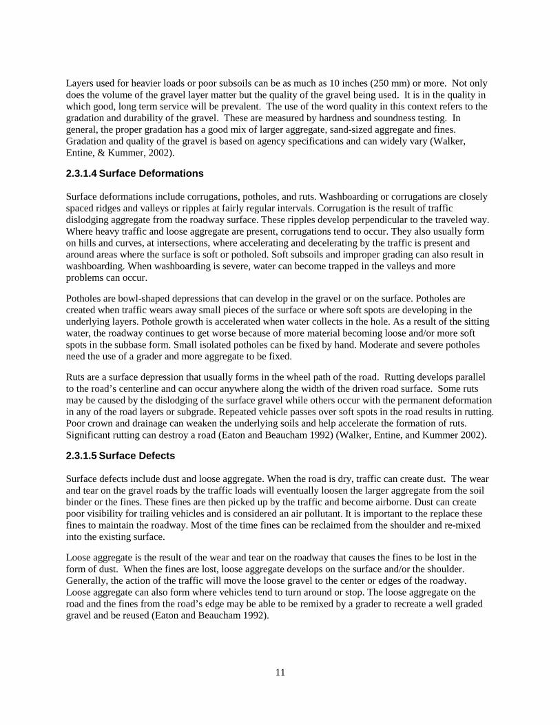
2.3.1.4 Surface Deformations Surface deformations include corrugations, potholes, and ruts. Washboarding or corrugations are closely spaced ridges and valleys or ripples at fairly regular intervals. Corrugation is the result of traffic dislodging aggregate from the roadway surface. These ripples develop perpendicular to the traveled way. Where heavy traffic and loose aggregate are present, corrugations tend to occur. They also usually form on hills and curves, at intersections, where accelerating and decelerating by the traffic is present and around areas where the surface is soft or potholed. Soft subsoils and improper grading can also result in washboarding. When washboarding is severe, water can become trapped in the valleys and more problems can occur.

Potholes are bowl-shaped depressions that can develop in the gravel or on the surface. Potholes are created when traffic wears away small pieces of the surface or where soft spots are developing in the underlying layers. Pothole growth is accelerated when water collects in the hole. As a result of the sitting water, the roadway continues to get worse because of more material becoming loose and/or more soft spots in the subbase form. Small isolated potholes can be fixed by hand. Moderate and severe potholes need the use of a grader and more aggregate to be fixed.

Ruts are a surface depression that usually forms in the wheel path of the road. Rutting develops parallel to the road’s centerline and can occur anywhere along the width of the driven road surface. Some ruts may be caused by the dislodging of the surface gravel while others occur with the permanent deformation in any of the road layers or subgrade. Repeated vehicle passes over soft spots in the road results in rutting. Poor crown and drainage can weaken the underlying soils and help accelerate the formation of ruts. Significant rutting can destroy a road (Eaton and Beaucham 1992) (Walker, Entine, and Kummer 2002).

2.3.1.5 Surface Defects Surface defects include dust and loose aggregate. When the road is dry, traffic can create dust. The wear and tear on the gravel roads by the traffic loads will eventually loosen the larger aggregate from the soil binder or the fines. These fines are then picked up by the traffic and become airborne. Dust can create poor visibility for trailing vehicles and is considered an air pollutant. It is important to the replace these fines to maintain the roadway. Most of the time fines can be reclaimed from the shoulder and re-mixed into the existing surface.

Loose aggregate is the result of the wear and tear on the roadway that causes the fines to be lost in the form of dust. When the fines are lost, loose aggregate develops on the surface and/or the shoulder. Generally, the action of the traffic will move the loose gravel to the center or edges of the roadway. Loose aggregate can also form where vehicles tend to turn around or stop. The loose aggregate on the road and the fines from the road’s edge may be able to be remixed by a grader to recreate a well graded gravel and be reused (Eaton and Beaucham 1992).

12

2.4 Dust Control There are strong reasons to control dust from unpaved roads. The top problem associated with unpaved roads is fugitive dust created by traffic and the loss of fines. Dust is considered as a type of particulate matter air pollution. It can contaminate houses and barns, it settles on vegetation and can reduce visibility over long distances. Dust is usually kicked up into the air by vehicles or blown off the road by wind. Not only is dust present on gravel roads, it is also generated by road construction and is a given at quarries and gravel pits. Also, the more dust that leaves the road surface, the less road surface that will remain. When dust is blown away, aggregates in the road surface loosen which can lead to many types of distresses and costly maintenance or rehabilitation efforts for the road departments as well as higher road user costs in the form of vehicle maintenance (Kuennen 2006) (Addo, Sanders, and Chenard 2004).

Dust is considered a coarse particle (PM-10), that is, dust is made up of particles that are 10 micrometers (microns) or less. Another way look at it is dust particles are about one-seventh of the diameter of a human hair. The EPA has had national air quality standards for PM-10 since 1987. These standards consist of a 24-hour standard not to exceed 150 micrograms per cubic meter of air, and an average standard of 50 micrograms per cubic meter annually (Kuennen 2006).

Scientific studies have linked particulate matter pollution with significant health problems such as:

• Increased respiratory symptoms like irritation of airways, coughing, and difficulty breathing • Decreased lung function • Aggravated asthma • Development of chronic bronchitis • Irregular heartbeat • Premature death of people with heart or lung disease

Coughing, wheezing and decreased lung function in healthy individuals can be caused by particle pollution (Kuennen 2006). The standards for dust exclude dust that occurs due to natural kick-up by the wind. It is not practical or feasible to place regulation on dust caused by the wind. On the other hand, it is possible to manage fugitive dust with dust control measures (Kuennen 2006).

2.4.1 Types of Dust Suppressants Dust control methods range from spraying the road with chemicals to using geotextiles in the reconstruction of a road. Other efforts may include reduction in vehicular speed and the application of water. The use of dust suppressants is justifiable when traffic is low and paving is not a feasible option financially, the cost of the suppressants and application are low, and when stage construction is planned. The commonly used dust suppressants are water, chloride compounds, lignin derivatives, and resinous adhesives. Performance characteristics as well as the type and volume of traffic, climate, roadway conditions and product cost all play a significant role in selecting a dust suppressant (Addo, Sanders, and Chenard 2004) (Sanders and Addo 1993).

The main idea behind dust suppression is to keep moisture in the surface of the roadway. Moisture keeps the dust particles wet which in turn increases their mass and cohesion. The moisture allows fines in the gravel to adhere to other fines as well as other aggregate in the mix. When the moisture content is sufficient, optimum compaction under the traffic load is achieved (Kuennen 2006).

13

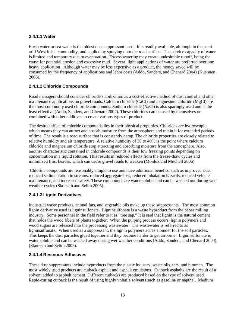
2.4.1.1 Water Fresh water or sea water is the oldest dust suppressant used. It is readily available, although in the semi-arid West it is a commodity, and applied by spraying onto the road surface. The service capacity of water is limited and temporary due to evaporation. Excess watering may create undesirable runoff, being the cause for potential erosion and excessive mud. Several light applications of water are preferred over one heavy application. Although water may be less expensive as a product, the money saved will be consumed by the frequency of applications and labor costs (Addo, Sanders, and Chenard 2004) (Kuennen 2006).

2.4.1.2 Chloride Compounds Road managers should consider chloride stabilization as a cost-effective method of dust control and other maintenance applications on gravel roads. Calcium chloride (CaCl) and magnesium chloride (MgCl) are the most commonly used chloride compounds. Sodium chloride (NaCl) is also sparingly used and is the least effective (Addo, Sanders, and Chenard 2004). These chlorides can be used by themselves or combined with other additives to create various types of product.

The desired effect of chloride compounds lies in their physical properties. Chlorides are hydroscopic, which means they can attract and absorb moisture from the atmosphere and retain it for extended periods of time. The result is a road surface that is constantly damp. The chloride properties are closely related to relative humidity and air temperature. A relative humidity of 30 to 40% is the point where calcium chloride and magnesium chloride stop attracting and absorbing moisture from the atmosphere. Also, another characteristic contained in chloride compounds is their low freezing points depending on concentration in a liquid solution. This results in reduced effects from the freeze-thaw cycles and minimized frost heaves, which can cause gravel roads to weaken (Monlux and Mitchell 2006).

Chloride compounds are reasonably simple to use and have additional benefits, such as improved ride, reduced sedimentation in streams, reduced aggregate loss, reduced inhalation hazards, reduced vehicle maintenance, and increased safety. These compounds are water soluble and can be washed out during wet weather cycles (Skorseth and Selim 2005).

2.4.1.3 Lignin Derivatives Industrial waste products, animal fats, and vegetable oils make up these suppressants. The most common lignin derivative used is ligninsulfonate. Ligninsulfonate is a waste byproduct from the paper milling industry. Some personnel in the field refer to it as “tree sap.” It is said that lignin is the natural cement that holds the wood fibers of plants together. When the pulping process occurs, lignin polymers and wood sugars are released into the processing wastewater. The wastewater is referred to as ligninsulfonate. When used as a suppressant, the lignin polymers act as a binder for the soil particles. This keeps the dust particles glued together and they become harder to get airborne. Ligninsulfonate is water soluble and can be washed away during wet weather conditions (Addo, Sanders, and Chenard 2004) (Skorseth and Selim 2005).

2.4.1.4 Resinous Adhesives These dust suppressants include byproducts from the plastic industry, waste oils, tars, and bitumen. The most widely used products are cutback asphalt and asphalt emulsions. Cutback asphalts are the result of a solvent added to asphalt cement. Different cutbacks are produced based on the type of solvent used. Rapid-curing cutback is the result of using highly volatile solvents such as gasoline or napthal. Medium

14

and slow-curing cutbacks are created when lighter solvents such as kerosene are used. Asphalt emulsions are created by dispersing asphalts as small droplets of water. This is achieved by adding an emulsifying agent during the process. When resinous adhesives are used as dust suppressants, they create the most durable, dust free surfaces. This is due to their high cohesive properties and their insolubility to water. The use of these products was once popular but the amounts of fuel oil or kerosene in these products along with rising fuel costs has resulted in declined use and is being banned in many places. These products need to be applied by special asphalt application equipment (Addo, Sanders, and Chenard 2004).

Clays have also been used a dust suppressants. Clays have high plasticity and strong cohesion and work well when added to gravel in the right proportions. It is hard to haul and mix clay with gravel due to its high plasticity. For tars and bitumens, the structure and composition of the aggregates is the major factor that affects their cohesion in aggregate-asphalt mixes. A byproduct of soybean oil refining is also used as a dust suppressant. It is biodegradable and has many characteristics of light petroleum based oils. This product will penetrate the surface and create a light bond that reduces dust. There are also many other commercial products that may be used and should be tested on small sections of roadway before full use is decided upon (Skorseth and Selim 2005).

2.5 Dust Collection and Measurement A majority of the research done with dust measurements has been focused in atmospheric pollution. Within the study of atmospheric pollution, dust measurements focus on two areas: 1) atmospheric modeling and prediction and 2) field measurement and quantification. The three main methods of air sampling techniques used by atmospheric pollution scientists are classified as sedimentation techniques, filtration techniques, and photometric techniques (Sanders and Addo 2000).

The sedimentation technique is a sampling method used for dust particle fallout from the atmosphere. These techniques follow ASTM D 1739 standards. Open-top containers, such as glass, metal, or plastic jars are used in this method. These containers have a height that is two to three times the diameter of the jar. Particulates are collected over an exposure period that is typically a month. The collected amount of particulate is expressed in terms of weight per unit area per 30 days. This technique depends on the forces of gravity and limits the particle size to about 2 µm or greater. There are a number of disadvantages to this technique as it requires an extended collection period for one sample, contaminated samples caused by foreign matter mixing with the collected dust, and the effect of winds on the samples (Sanders and Addo 2000).

The filtration technique employs the use of a suction source under a filter. The type of filter and the sampling equipment is dependent on the desired data and type of test being performed. An example of device that uses the filtration technique is the high volumetric sampler. The major drawback of this technique is that it requires the use of electric power to run the suction pump (Sanders and Addo 2000).

The photometric technique is based on the absorption properties of particulates passing though a light source. Basically, this technique looks at the light scattering as a sample passes through a light source. The amount of light scattered is dependent on the concentration, size, refractive index, shape, and color of the suspended particles.

The devices and techniques developed to measure road dust employ one or more of these particulate sampling techniques. In 1972, Wellman and Barraclough used the photometric technique to measure dust concentrations at a point along an unpaved road. Research performed by Hoover et al. in 1973 used the sedimentation technique by installing cups on the roadside of unpaved roads to gain data on the nature of dust generation and distribution. In 1984, Langon built a portable cyclone dust collector and mounted it on the rear of dust generating vehicle. The goal of this research was to use the filtration technique over a

15

section of the road versus one point on the road. In 1986, the USDA Forest Service, in a cooperative study with Irwin et al. at Cornell University, developed a device that measured the road dust in terms of air opacity using photometric techniques. This device was called the Road Dust Monitor (RDM).

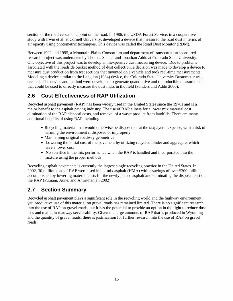
Between 1992 and 1995, a Mountain-Plains Consortium and department of transportation sponsored research project was undertaken by Thomas Sander and Jonathan Addo at Colorado State University. One objective of this project was to develop an inexpensive dust measuring device. Due to problems associated with the roadside bucket method of dust collection, a decision was made to develop a device to measure dust production from test sections that mounted on a vehicle and took real-time measurements. Modeling a device similar to the Langdon (1984) device, the Colorado State University Dustometer was created. The device and method were developed to generate quantitative and reproducible measurements that could be used to directly measure the dust mass in the field (Sanders and Addo 2000).

2.6 Cost Effectiveness of RAP Utilization Recycled asphalt pavement (RAP) has been widely used in the United States since the 1970s and is a major benefit to the asphalt paving industry. The use of RAP allows for a lower mix material cost, elimination of the RAP disposal costs, and removal of a waste product from landfills. There are many additional benefits of using RAP including:

• Recycling material that would otherwise be disposed of at the taxpayers’ expense, with a risk of harming the environment if disposed of improperly

• Maintaining original roadway geometrics • Lowering the initial cost of the pavement by utilizing recycled binder and aggregate, which

have a lower cost • No sacrifice in the mix performance when the RAP is handled and incorporated into the

mixture using the proper methods

Recycling asphalt pavements is currently the largest single recycling practice in the United States. In 2002, 30 million tons of RAP were used in hot mix asphalt (HMA) with a savings of over $300 million, accomplished by lowering material costs for the newly placed asphalt and eliminating the disposal cost of the RAP (Putnam, Aune, and Amirkhanian 2002).

2.7 Section Summary Recycled asphalt pavement plays a significant role in the recycling world and the highway environment, yet, productive use of this material on gravel roads has remained limited. There is no significant research into the use of RAP on gravel roads, but it has the potential to provide an option in the fight to reduce dust loss and maintain roadway serviceability. Given the large amounts of RAP that is produced in Wyoming and the quantity of gravel roads, there is justification for further research into the use of RAP on gravel roads.

16

17

3. DESIGN OF STUDY AND TESTING PROCEDURES

3.1 Introduction The objective of this research project was to explore the use of Recycled Asphalt Pavement (RAP) in gravel roads to help reduce dust loss while maintaining roadway serviceability. To accomplish this objective, field experiments were constructed in two counties in the state of Wyoming. Laramie County and Johnson County obtained RAP from WYDOT to use on some sections in their unpaved road network. The design of the sections utilizing RAP was developed by the individual county’s road and bridge department in conjunction with the WYT2 center.

Each section had three monitoring activities performed on them during the summer of 2008. Dust collection was taken using the Colorado State University (CSU) Dustometer. Surface distresses were observed following an established United States Army Corps of Engineers method. Roadway moisture content and wind characteristics were also collected on all sections. Laboratory testing was also performed by WYDOT on the materials used in the test sections. From these activities, the performance of RAP in gravel roads was evaluated.

3.2 Data Collection and Laboratory Testing

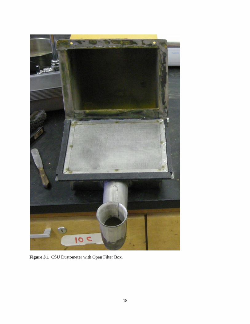
3.2.1 CSU Dustometer Dust monitoring was accomplished using the CSU Dustometer. The Dustometer is a dust collection device that attaches behind the driver side rear wheel of the test vehicle. The Dustometer is an inexpensive moving dust sampler that was developed at CSU by Thomas Sanders and Jonathan Addo. It has been proven to be a quantitative, reproducible, and precise device for dust measurement (Sanders and Addo 1993).

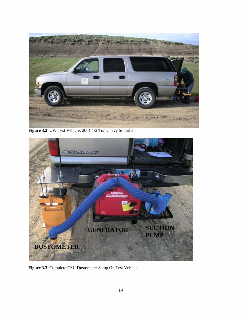
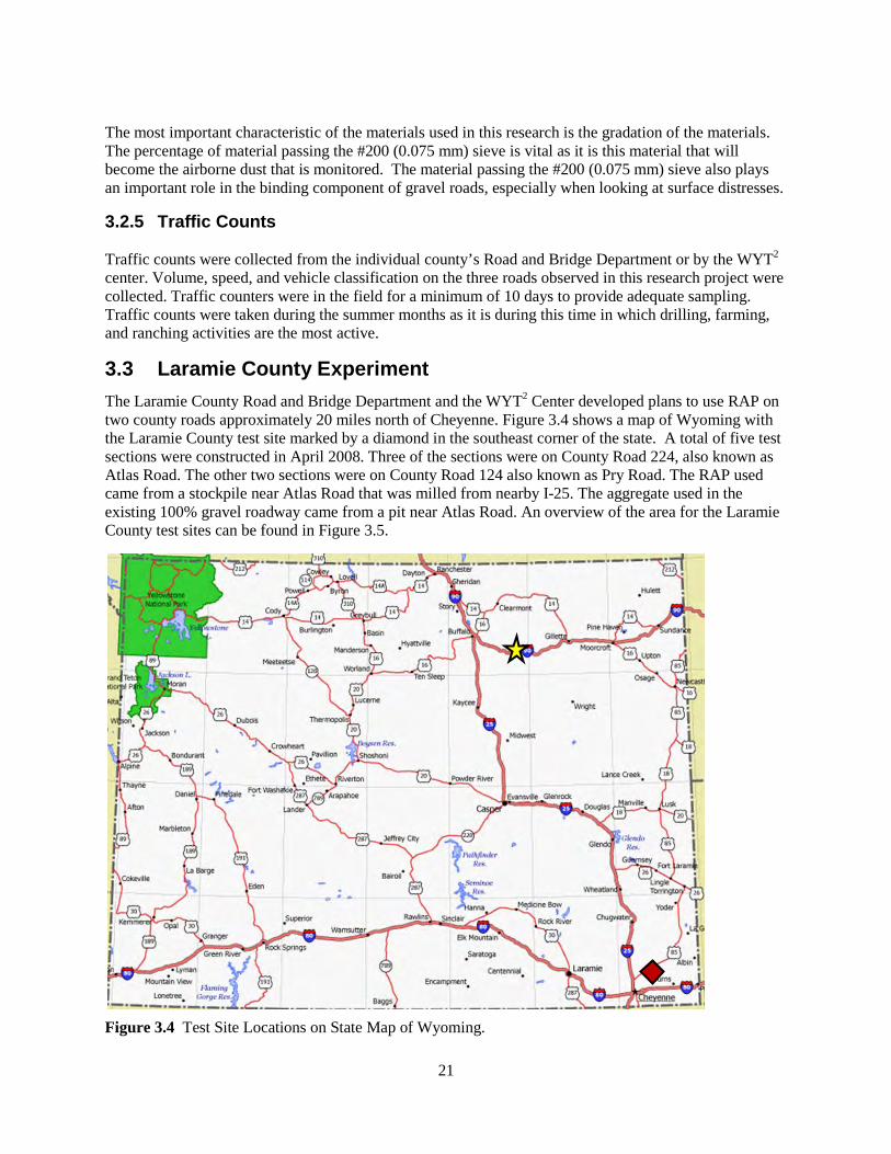
The device consists of a fabricated steel filter box that contains glass microfiber filters; a standard high volumetric suction pump; a steel mounting bracket attached to the bumper of the test vehicle; a flexible hose for connecting the suction pump to the filter box; a gas-powered generator; an on/off switchbox for the suction pump; and a 2001 Chevy Suburban used as a testing vehicle. The steel filter box has an opening facing the rear wheel covered with a 200 µm mesh sieve screen that prevents large particles from entering the box during collection. The bottom of the filter box opens to allow access to the filter paper, which rests on another 200 µm mesh sieve screen that is mounted horizontally in the filter box (Morgan, Schaefer, and Sharma 2005). Figure 3.1 shows the CSU Dustometer with the clam shell open. Figures 3.2 and 3.3 show the University of Wyoming test vehicle setup.

18

Figure 3.1 CSU Dustometer with Open Filter Box.

19

Figure 3.2 UW Test Vehicle: 2001 1/2 Ton Chevy Suburban.

Figure 3.3 Complete CSU Dustometer Setup On Test Vehicle.

DUSTOMETER

GENERATOR SUCTION PUMP

20

For each test, the 2001 half-ton Chevy Suburban was run at a test speed of 40 mph (64 km/hr) with a tire pressure of 50 psi (345 kPA) over one-half mile of the test section. Whatman EPM 2000 glass Microfibre filters were used. Dust data were collected by (1) weighing inside a gallon Baggie and recording; (2) setting up the Dustometer and making a run at 40 mph; (3) collecting the filter and sample in original gallon Baggie; and (4) re-weighing the Baggie with sample to find the dust sample weight in grams. All test sections had one dust measurement taken from each direction.

3.2.2 Environmental Factors Environmental factors were collected on each section every time a dust measurement was taken. These factors include wind speed, wind direction, and surface moisture content. The wind characteristics were collected on site using a hand held compass and wind vane. The WindMate 200 by Speedtech Industries was used to collect this data. Road surface moisture content was collected by scraping off a sample of the road surface using a pick. A depth of no more than one inch (25 mm) was scraped off the surface and collected in a tin can. The tin can was taped off to seal in the moisture and returned to the lab. Each sample was weighed before and after drying, and the moisture content was calculated. Moisture content, wind speed, and wind direction were collected every time a dust measurement was performed.

3.2.3 Distress Survey Surface distresses of each section were found using the methods presented in Unsurfaced Road Maintenance Management by Robert A. Eaton and Ronald E. Beaucham, USACE-CRREL Special Report 92-26, December 1992. A representative subsection of each test section (usually 100 feet) was determined and marked for monitoring. Each subsection was walked and all distresses were record every time field data were collected. The individual distresses were ranked according to the USACE methods, and a total unsurfaced road condition index (URCI) was established. The surface distresses were recorded on a field sheet that was developed by the USACE.

3.2.4 Material Characteristics Samples of the materials used were collected. These samples were taken to the WYDOT Materials Testing Lab to be properly tested. Various tests were performed on the materials to determine the desired characteristics of a given material. The laboratory testing results were used to describe the materials and their relation to dust loss and surface distresses as described in Section 5.

Samples of RAP and RAP blends from the individual counties were collected from stockpiles using proper sample collection techniques. These samples were bagged, tagged and transferred to the WYDOT Materials Testing Lab in Cheyenne, WY. Lab technicians performed the necessary tests on the RAP and RAP blend materials to find the following characteristics of the material: gradation, R-value, oil percentage, and gradation after extraction of oil.

Samples of virgin aggregate from the individual counties were collected from stockpiles or the pit using proper sample collection techniques. These samples were transferred to the WYDOT Materials Testing Lab. Lab technicians performed the necessary tests on the virgin aggregate to find the following characteristics of the material: gradation, Atterburg Limits, cohesion value, fractured faces, R-value, along with the percentage of gravel, sand silt and clay.

21

The most important characteristic of the materials used in this research is the gradation of the materials. The percentage of material passing the #200 (0.075 mm) sieve is vital as it is this material that will become the airborne dust that is monitored. The material passing the #200 (0.075 mm) sieve also plays an important role in the binding component of gravel roads, especially when looking at surface distresses.

3.2.5 Traffic Counts Traffic counts were collected from the individual county’s Road and Bridge Department or by the WYT2 center. Volume, speed, and vehicle classification on the three roads observed in this research project were collected. Traffic counters were in the field for a minimum of 10 days to provide adequate sampling. Traffic counts were taken during the summer months as it is during this time in which drilling, farming, and ranching activities are the most active.

3.3 Laramie County Experiment The Laramie County Road and Bridge Department and the WYT2 Center developed plans to use RAP on two county roads approximately 20 miles north of Cheyenne. Figure 3.4 shows a map of Wyoming with the Laramie County test site marked by a diamond in the southeast corner of the state. A total of five test sections were constructed in April 2008. Three of the sections were on County Road 224, also known as Atlas Road. The other two sections were on County Road 124 also known as Pry Road. The RAP used came from a stockpile near Atlas Road that was milled from nearby I-25. The aggregate used in the existing 100% gravel roadway came from a pit near Atlas Road. An overview of the area for the Laramie County test sites can be found in Figure 3.5.

Figure 3.4 Test Site Locations on State Map of Wyoming.

22

Figure 3.5 Overview of Laramie County Test Site.

Of the five total test sections in Laramie County, three consisted of blended RAP and gravel while the other two contained 100% gravel to be used as control sections. The RAP blend sections were all blended on site. The construction process consisted of (1) scarifying the existing 100% gravel roadway with a motor grader, (2) hauling and dumping a calculated volumetric depth of pure RAP onto the scarified roadway, (3) blending the RAP and aggregate using the blade on a motor grader, (4) shaping the road with the newly created RAP blend, and (5) letting traffic compact the roadway. No additional dust abatement measures were taken on the test sections.

The results of construction on Atlas Road consisted of three sections: two different RAP blends and one 100% gravel control. One RAP blend section consisted of a volumetric depth of 2½ inches (62.5 mm) of RAP blended with the existing surface. The total length of the section was 0.6 miles, and it was named A2. The other RAP blend section consisted of a volumetric depth of 1½ inches (37.5 mm) of RAP blended with the existing surface. The total length of the section was 0.7 miles, and it was named A1.

23

Finally, the remaining 0.7 miles of Atlas Road consisted of 100% gravel. This control section was named A0. Figure 3.6 shows the test sections on Atlas Road.

Figure 3.6 Atlas Road Test Sections. The results of construction on Pry Road consisted of two sections: one RAP blend and one 100% gravel control. The RAP blend section consisted of a volumetric depth of 1½ inches (37.5 mm) of RAP blended with the existing surface. The total length of the section was 0.8 miles, and it was named P1. The 100% gravel control section had a length of 1.2 miles, and was named P0. Figure 3.7 shows the test sections on Pry Road.

Figure 3.7 Test Sections on Pry Road.

24

Although each test section in Laramie County was longer than one-half mile, only one-half of a mile was used for testing. The beginning and end of each half mile test section was clearly marked using painted wood stakes in the ditch and brightly colored tape on the fence line. Field data were collected and monitored on each section independently.

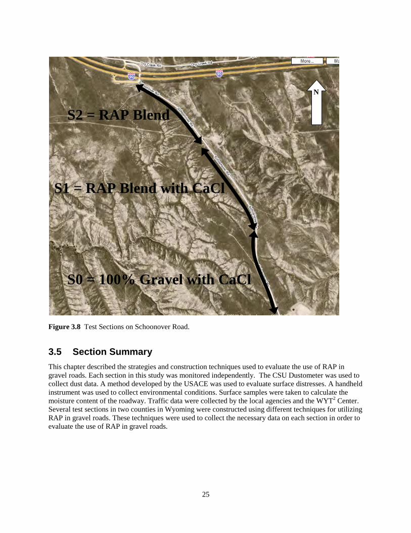
3.4 Johnson County Experiment The Johnson County Road and Bridge Department and the WYT2 Center developed plans to use RAP on Schoonover Road approximately 20 miles east of Buffalo, WY. Figure 3.4 above shows a map of the State of Wyoming with the Johnson County test site marked by a star in the northern part of the state. A total of three sections were constructed in June 2008. All three sections were constructed back to back. Two contained RAP blends and the third was a 100% gravel control. The addition of calcium chloride (CaCl) was used on two of the test sections.

The construction process in Johnson County was much different than that in Laramie County. The construction process on Schoonover Road consisted of (1) mixing RAP with virgin aggregate off-site in a pugmill with a 1 to 1 ratio resulting in 50% RAP and 50% virgin aggregate blend; (2) hauling the RAP blend onto site and dumping on the existing roadway; (3) using the blade on a motor grader to spread the RAP blend and shape the roadway; and (4) using a vibratory drum roller to compact the roadway surface.

Two weeks after construction, CaCl was applied to the appropriate sections. This process consisted of (1) wetting the roadway surface using a water truck; (2) spreading CaCl flakes on the wet roadway; (3) making another pass with the water truck; and (4) letting the CaCl leach into the roadway surface as the water dries off. CaCl was applied to one RAP blend section and the rest of the existing 100% gravel road.

The result of construction was three test sections. All the sections had a length of one-half mile. One section was a RAP blend section with no CaCl applied, and it was named S2. Another section was a RAP blend section with CaCl, and it was named S1. Finally, the third section was the 100% gravel with CaCl control section, and it was named S0. A section of 100% gravel without CaCl was not constructed due the heavy traffic experienced on Schoonover Road, especially truck traffic. Field data were collected and monitored on each section independently. Figure 3.8 gives a visual overview of the Johnson County test sections on Schoonover Road.

25

Figure 3.8 Test Sections on Schoonover Road.

3.5 Section Summary This chapter described the strategies and construction techniques used to evaluate the use of RAP in gravel roads. Each section in this study was monitored independently. The CSU Dustometer was used to collect dust data. A method developed by the USACE was used to evaluate surface distresses. A handheld instrument was used to collect environmental conditions. Surface samples were taken to calculate the moisture content of the roadway. Traffic data were collected by the local agencies and the WYT2 Center. Several test sections in two counties in Wyoming were constructed using different techniques for utilizing RAP in gravel roads. These techniques were used to collect the necessary data on each section in order to evaluate the use of RAP in gravel roads.

S2 = RAP Blend

S1 = RAP Blend with CaCl

S0 = 100% Gravel with CaCl

N

26

27

4. DATA COLLECTION

4.1 Introduction Field and laboratory data were collected in this research project to evaluate the performance of RAP in gravel roads. The field evaluation was accomplished by observing and collecting data on the test sections constructed in Laramie and Johnson Counties. Traffic data were provided by the individual county or the WYT2 Center. Dust measurements, surface surveys, and environmental factors were collected by the WYT2 Center.

The laboratory testing of material was conducted by the WYDOT Materials Testing Lab in Cheyenne, WY. Lab technicians performed the necessary tests on the materials to provide the desired characteristics of the material. One of the main purposes of this testing was to provide the gradations of the various materials. The tests performed followed the appropriate AASHTO and ASTM testing procedures. Wyoming modified AASHTO and ASTM testing procedures were used where applicable.

4.2 Material Characteristics To determine the characteristics of the materials used in this project, lab testing performed by WYDOT was utilized. All materials had a sieve analysis performed to determine the gradation of the material. Materials that contained RAP had different tests than the virgin aggregates due to the nature of the material and the testing. The following sections will break down the results of the lab testing.

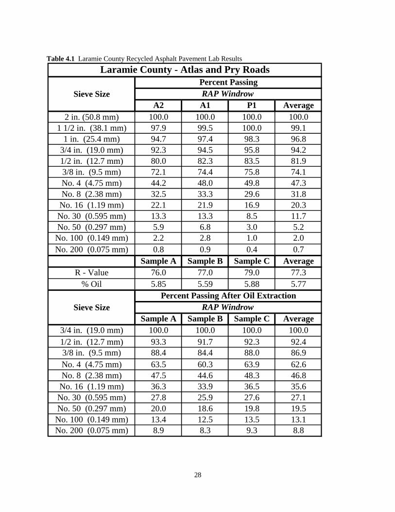
4.2.1 Recycled Asphalt Pavement RAP samples were collected for both Laramie and Johnson Counties. Gradation before and after extraction of the oil was desired, along with the R-value for strength of the material and the percentage of oil in the RAP. Table 4.1 summarizes the laboratory results for the RAP used in Laramie County. Figure 4.1 shows the gradation of the RAP used in Laramie County. No samples of the RAP used in Johnson County were taken as all of the material used was already blended with 100% virgin aggregate. Please refer to Appendix C for the complete data set.

From the laboratory results and gradation, it can be seen that the RAP material has less than 1% of the total material passing the #200 (0.075mm) sieve. Therefore, the amount of fines found in the RAP material is very small. Also, from Figure 4.1 it can be seen that the RAP is well graded. These characteristics make the RAP a suitable addition to gravel roads for reducing dust loss.

28

Table 4.1 Laramie County Recycled Asphalt Pavement Lab Results

A2 A1 P1 Average2 in. (50.8 mm) 100.0 100.0 100.0 100.0

1 1/2 in. (38.1 mm) 97.9 99.5 100.0 99.11 in. (25.4 mm) 94.7 97.4 98.3 96.8

3/4 in. (19.0 mm) 92.3 94.5 95.8 94.21/2 in. (12.7 mm) 80.0 82.3 83.5 81.93/8 in. (9.5 mm) 72.1 74.4 75.8 74.1No. 4 (4.75 mm) 44.2 48.0 49.8 47.3No. 8 (2.38 mm) 32.5 33.3 29.6 31.8

No. 16 (1.19 mm) 22.1 21.9 16.9 20.3No. 30 (0.595 mm) 13.3 13.3 8.5 11.7No. 50 (0.297 mm) 5.9 6.8 3.0 5.2

No. 100 (0.149 mm) 2.2 2.8 1.0 2.0No. 200 (0.075 mm) 0.8 0.9 0.4 0.7

Sample A Sample B Sample C AverageR - Value 76.0 77.0 79.0 77.3

% Oil 5.85 5.59 5.88 5.77

Sample A Sample B Sample C Average3/4 in. (19.0 mm) 100.0 100.0 100.0 100.01/2 in. (12.7 mm) 93.3 91.7 92.3 92.43/8 in. (9.5 mm) 88.4 84.4 88.0 86.9No. 4 (4.75 mm) 63.5 60.3 63.9 62.6No. 8 (2.38 mm) 47.5 44.6 48.3 46.8

No. 16 (1.19 mm) 36.3 33.9 36.5 35.6No. 30 (0.595 mm) 27.8 25.9 27.6 27.1No. 50 (0.297 mm) 20.0 18.6 19.8 19.5

No. 100 (0.149 mm) 13.4 12.5 13.5 13.1No. 200 (0.075 mm) 8.9 8.3 9.3 8.8

RAP WindrowSieve SizePercent Passing After Oil Extraction

Laramie County - Atlas and Pry Roads

Sieve SizePercent PassingRAP Windrow

29

Figure 4.1 Gradation of RAP Material Used in Laramie County.

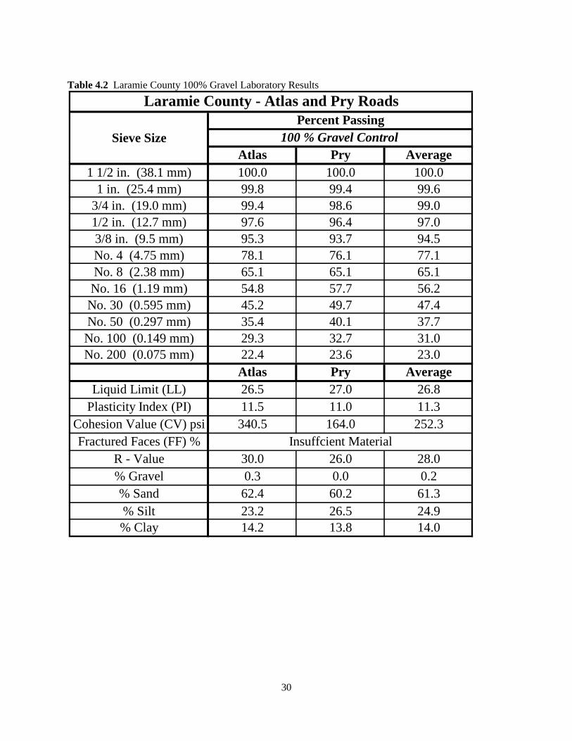
4.2.2 Virgin Aggregate Virgin aggregate samples were collected for both Laramie County and Johnson County. Gradation, Atterburg Limits, cohesion value, fractured faces, R-value, percentage of gravel, sand, silt, and clay were determined. Table 4.2 summarizes the lab results for the virgin aggregate used in Laramie County and Table 4.3 summarizes the lab results for the virgin aggregate used in Johnson County. Figure 4.2 contains the gradations of the gravel used in Laramie and Johnson Counties. Please refer to Appendix C for the complete data set.

0

10

20

30

40

50

60

70

80

90

100

0.00.11.010.0100.0

Perc

ent P

assi

ng (%

)

Sieve Size (mm)

Laramie County RAP Gradation

30

Table 4.2 Laramie County 100% Gravel Laboratory Results

Atlas Pry Average1 1/2 in. (38.1 mm) 100.0 100.0 100.0

1 in. (25.4 mm) 99.8 99.4 99.63/4 in. (19.0 mm) 99.4 98.6 99.01/2 in. (12.7 mm) 97.6 96.4 97.03/8 in. (9.5 mm) 95.3 93.7 94.5No. 4 (4.75 mm) 78.1 76.1 77.1No. 8 (2.38 mm) 65.1 65.1 65.1

No. 16 (1.19 mm) 54.8 57.7 56.2No. 30 (0.595 mm) 45.2 49.7 47.4No. 50 (0.297 mm) 35.4 40.1 37.7

No. 100 (0.149 mm) 29.3 32.7 31.0No. 200 (0.075 mm) 22.4 23.6 23.0

Atlas Pry AverageLiquid Limit (LL) 26.5 27.0 26.8

Plasticity Index (PI) 11.5 11.0 11.3Cohesion Value (CV) psi 340.5 164.0 252.3Fractured Faces (FF) %

R - Value 30.0 26.0 28.0% Gravel 0.3 0.0 0.2% Sand 62.4 60.2 61.3% Silt 23.2 26.5 24.9% Clay 14.2 13.8 14.0

Laramie County - Atlas and Pry RoadsPercent Passing

100 % Gravel Control

Insuffcient Material

Sieve Size

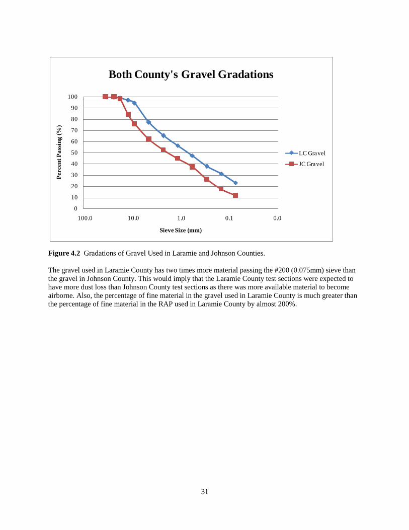
31

Figure 4.2 Gradations of Gravel Used in Laramie and Johnson Counties. The gravel used in Laramie County has two times more material passing the #200 (0.075mm) sieve than the gravel in Johnson County. This would imply that the Laramie County test sections were expected to have more dust loss than Johnson County test sections as there was more available material to become airborne. Also, the percentage of fine material in the gravel used in Laramie County is much greater than the percentage of fine material in the RAP used in Laramie County by almost 200%.

0

10

20

30

40

50

60

70

80

90

100

0.00.11.010.0100.0

Perc

ent P

assi

ng (%

)

Sieve Size (mm)

Both County's Gravel Gradations

LC Gravel

JC Gravel

32

Table 4.3 Johnson County 100% Virgin Aggregate Laboratory Results

4.2.3 RAP Blend RAP blend samples were collected for both Laramie County and Johnson County. Gradation before and after extraction of the oil were desired along with the R-value for strength of the material and the percentage of oil in the RAP blend. Table 4.4 summarizes the lab results for the RAP blend used in Laramie County and Table 4.5 summarizes the lab results for the RAP blend used in Johnson County. Figure 4.3 contains the gradations of the RAP blends used in Laramie and Johnson Counties. Please refer to Appendix C for the complete data set.

Sample A Sample B Sample C Average1 1/2 in. (38.1 mm) 100.0 100.0 100.0 100.0

1 in. (25.4 mm) 100.0 100.0 99.8 99.93/4 in. (19.0 mm) 98.0 98.4 98.0 98.11/2 in. (12.7 mm) 83.5 86.0 82.5 84.03/8 in. (9.5 mm) 75.7 77.7 73.8 75.7No. 4 (4.75 mm) 62.1 63.7 60.6 62.1No. 8 (2.38 mm) 50.5 53.9 52.8 52.4

No. 16 (1.19 mm) 42.8 46.0 45.5 44.8No. 30 (0.595 mm) 35.8 38.2 38.0 37.3No. 50 (0.297 mm) 25.7 26.4 26.3 26.1

No. 100 (0.149 mm) 17.0 17.4 17.4 17.3No. 200 (0.075 mm) 11.5 11.3 12.0 11.6

Sample A Sample B Sample C AverageLiquid Limit (LL) NV NV NV NV

Plasticity Index (PI) NP NP NP NPCohesion Value (CV) psi 517.0 400.0 420.0 445.7Fractured Faces (FF) % 89.1 91.6 90.2 90.3

R - Value 74.0 79.0 71.0 74.7% Gravel 0.0 0.3 0.4 0.2% Sand 75.3 72.1 78.8 75.4% Silt 18.7 21.4 14.9 18.3% Clay 6.0 6.2 5.9 6.0

Percent PassingStockpiled Virgin AggregateSieve Size

Johnson County - Schoonover Road

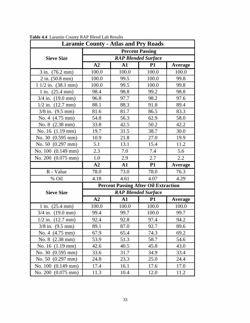
33

Table 4.4 Laramie County RAP Blend Lab Results

A2 A1 P1 Average3 in. (76.2 mm) 100.0 100.0 100.0 100.02 in. (50.8 mm) 100.0 99.5 100.0 99.8

1 1/2 in. (38.1 mm) 100.0 99.5 100.0 99.81 in. (25.4 mm) 98.4 98.8 99.2 98.8

3/4 in. (19.0 mm) 96.8 97.7 98.2 97.61/2 in. (12.7 mm) 88.1 88.3 91.8 89.43/8 in. (9.5 mm) 81.6 81.7 86.5 83.3No. 4 (4.75 mm) 54.8 56.3 62.9 58.0No. 8 (2.38 mm) 33.8 42.5 50.2 42.2

No. 16 (1.19 mm) 19.7 31.5 38.7 30.0No. 30 (0.595 mm) 10.9 21.8 27.0 19.9No. 50 (0.297 mm) 5.1 13.1 15.4 11.2

No. 100 (0.149 mm) 2.3 7.0 7.4 5.6No. 200 (0.075 mm) 1.0 2.9 2.7 2.2

A2 A1 P1 AverageR - Value 78.0 73.0 78.0 76.3

% Oil 4.18 4.61 4.07 4.29

A2 A1 P1 Average1 in. (25.4 mm) 100.0 100.0 100.0 100.0

3/4 in. (19.0 mm) 99.4 99.7 100.0 99.71/2 in. (12.7 mm) 92.4 92.8 97.4 94.23/8 in. (9.5 mm) 89.1 87.0 92.7 89.6No. 4 (4.75 mm) 67.9 65.4 74.3 69.2No. 8 (2.38 mm) 53.9 51.3 58.7 54.6

No. 16 (1.19 mm) 42.6 40.5 45.8 43.0No. 30 (0.595 mm) 33.6 31.7 34.9 33.4No. 50 (0.297 mm) 24.8 23.3 25.0 24.4

No. 100 (0.149 mm) 17.4 16.1 17.6 17.0No. 200 (0.075 mm) 11.3 10.4 12.0 11.2

Percent Passing After Oil ExtractionRAP Blended SurfaceSieve Size

Laramie County - Atlas and Pry Roads

Sieve SizePercent Passing

RAP Blended Surface

34

Figure 4.3 Gradations of RAP Blend Used in Laramie and Johnson Counties. The percentage of RAP blend material that passed the #200 (0.075mm) sieve was greater for Laramie County compared with Johnson County by 220%. This suggests that the RAP blended sections in Laramie County should have more dust loss than those in Johnson County.

0

10

20

30

40

50

60

70

80

90

100

0.00.11.010.0100.0

Perc

ent P

assi

ng (%

)

Sieve Size (mm)

Both County's RAP Blend Gradations

LC RAP Blend

JC RAP Blend

35

Table 4.5 Johnson County RAP Blend Lab Results

Sample A Sample B Sample C Average2 in. (50.8 mm) 100 100 100 100

1 1/2 in. (38.1 mm) 99.5 100.0 99.4 99.61 in. (25.4 mm) 97.0 98.5 96.5 97.3

3/4 in. (19.0 mm) 91.8 94.4 90.8 92.31/2 in. (12.7 mm) 76.6 80.2 74.7 77.23/8 in. (9.5 mm) 68.1 71.6 66.1 68.6No. 4 (4.75 mm) 48.4 48.9 47.4 48.2No. 8 (2.38 mm) 36.0 28.2 33.1 32.4No. 16 (1.19 mm) 23.3 14.0 20.9 19.4No. 30 (0.595 mm) 12.5 6.8 11.0 10.1No. 50 (0.297 mm) 4.8 3.5 4.5 4.3No. 100 (0.149 mm) 1.8 1.9 1.8 1.8No. 200 (0.075 mm) 0.7 1.5 0.8 1.0

Sample A Sample B Sample C AverageR - Value 78.0 79.0 80.0 79.0

% Oil 2 2.4 2.15 2.2

Sample A Sample B Sample C Average1 in. (25.4 mm) 100.0 100.0 100.0 100.0

3/4 in. (19.0 mm) 100.0 98.2 97.3 98.51/2 in. (12.7 mm) 83.7 80.6 78.7 81.03/8 in. (9.5 mm) 76.5 73.3 78.7 76.2No. 4 (4.75 mm) 56.9 55.9 53.3 55.4No. 8 (2.38 mm) 46.7 47.9 45.2 46.6No. 16 (1.19 mm) 34.7 38.5 35.5 36.2No. 30 (0.595 mm) 24.6 29.0 25.6 26.4No. 50 (0.297 mm) 16.4 19.0 16.4 17.3No. 100 (0.149 mm) 10.3 11.8 9.8 10.6No. 200 (0.075 mm) 7.2 7.2 5.7 6.7

Sieve SizePercent Passing After Oil Extraction

RAP Virgin Blend

Johnson County - Schoonover Road

Sieve SizePercent Passing

RAP Virgin Blend

36

4.2.4 Material Comparison to WYDOT Gradation Requirements Table 4.6 contains a summary of the materials used in the test sections. Table 4.6 also contains the gradation requirements for gravel roads (Grading GR) from the WYDOT Standard Specifications for Road and Bridge Construction, 2003 Edition. The gradations of the RAP blends consist of the materials after the oil was chemically extracted. The RAP blends after chemical extraction in both counties are within specifications for WYDOT Grading GR, except that the one-half inch (12.7mm) material in Laramie County is a little high. This has no particular influence on dust loss or road serviceability as it the material smaller than the #4 (4.75 mm) sieve that is important. The gravel used in Johnson County meets the Grading GR specifications with the exception of the #30 (0.595mm) material having 37.3%, passing while the high end of the specification is 35% passing. The gravel used in Laramie County is on the high end of the Grading GR specifications with the majority of the materials not falling within the specification range. This is important when looking at the fines, especially the #200 (0.075mm) sieve, because there is more material available to be lost as dust. This will lead to more dust loss in Laramie County compared with Johnson County.

Table 4.6 Summary of Gradations and WYDOT Grading GR Specifications

4.2.5 Materials on the Test Sections Table 4.7 gives the gradations of the roadway surfaces that were used in both counties. Both Laramie and Johnson County had test sections with 100% gravel and RAP blends. The gradations of the RAP blended material are before chemical extraction of the oil was performed. The amount of material passing the #200 (0.075mm) sieve for the gravel used in Laramie County is twice as much as that in Johnson County. This also holds true for the RAP blended sections. The result will be more material available to be lost as dust in Laramie County than in Johnson County. Also, the amount of fines in the RAP blends is minimal as there is asphalt cement within the blend that is binding the materials together and making the blend suitable for application on gravel roads.

Laramie County Gravel

Laramie County RAP Blend After Extraction

Johnson County Gravel

Johnson County RAP Blend After Extraction

WYDOT Grading GR

1 1/2 in. (38.1 mm) 100.0 100.0 100.0 100.01 in. (25.4 mm) 99.6 100.0 99.9 100.0 100.0

3/4 in. (19.0 mm) 99.0 99.7 98.1 98.5 90 to 1001/2 in. (12.7 mm) 97.0 94.2 84.0 81.0 65 to 853/8 in. (9.5 mm) 94.5 89.6 75.7 76.2No. 4 (4.75 mm) 77.1 69.2 62.1 55.4 50 to 78No. 8 (2.38 mm) 65.1 54.6 52.4 46.6 37 to 67No. 16 (1.19 mm) 56.2 43.0 44.8 36.2No. 30 (0.595 mm) 47.4 33.4 37.3 26.4 13 to 35No. 50 (0.297 mm) 37.7 24.4 26.1 17.3No. 100 (0.149 mm) 31.0 17.0 17.3 10.6No. 200 (0.075 mm) 23.0 11.2 11.6 6.7 4 to 15

Percent Passing

Sieve Size

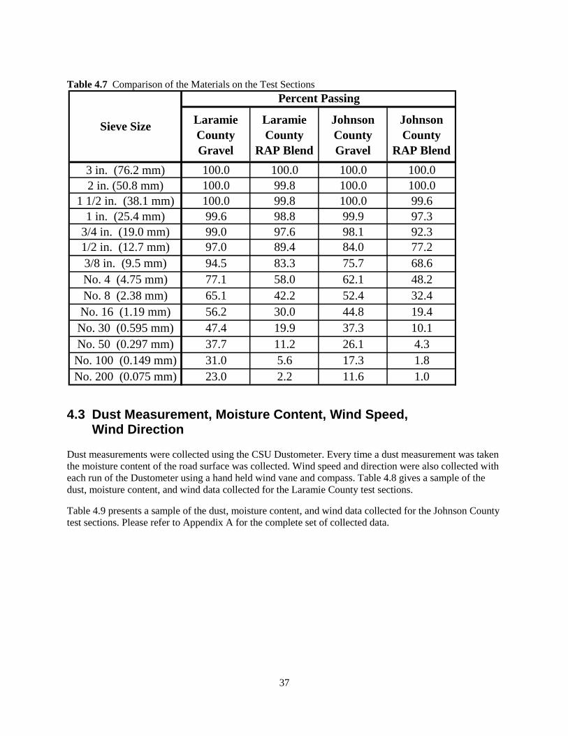
37

Table 4.7 Comparison of the Materials on the Test Sections

4.3 Dust Measurement, Moisture Content, Wind Speed, Wind Direction

Dust measurements were collected using the CSU Dustometer. Every time a dust measurement was taken the moisture content of the road surface was collected. Wind speed and direction were also collected with each run of the Dustometer using a hand held wind vane and compass. Table 4.8 gives a sample of the dust, moisture content, and wind data collected for the Laramie County test sections.

Table 4.9 presents a sample of the dust, moisture content, and wind data collected for the Johnson County test sections. Please refer to Appendix A for the complete set of collected data.

Laramie County Gravel

Laramie County

RAP Blend

Johnson County Gravel

Johnson County

RAP Blend3 in. (76.2 mm) 100.0 100.0 100.0 100.02 in. (50.8 mm) 100.0 99.8 100.0 100.0

1 1/2 in. (38.1 mm) 100.0 99.8 100.0 99.61 in. (25.4 mm) 99.6 98.8 99.9 97.3

3/4 in. (19.0 mm) 99.0 97.6 98.1 92.31/2 in. (12.7 mm) 97.0 89.4 84.0 77.23/8 in. (9.5 mm) 94.5 83.3 75.7 68.6No. 4 (4.75 mm) 77.1 58.0 62.1 48.2No. 8 (2.38 mm) 65.1 42.2 52.4 32.4No. 16 (1.19 mm) 56.2 30.0 44.8 19.4No. 30 (0.595 mm) 47.4 19.9 37.3 10.1No. 50 (0.297 mm) 37.7 11.2 26.1 4.3No. 100 (0.149 mm) 31.0 5.6 17.3 1.8No. 200 (0.075 mm) 23.0 2.2 11.6 1.0

Sieve Size

Percent Passing

38

Table 4.8 Sample of Dust, Wind, and Moisture Data Collected in Laramie County

Table 4.9 Sample of Dust, Wind, and Moisture Data Collected in Johnson County

1 Atlas Road - A2 (2 1/2" RAP) 6/9/2008 7:55 AM 20 W 1.82 2.0442 Atlas Road - A1 (1 1/2" RAP) 6/9/2008 8:10 AM 20 W 6.20 0.9913 Atlas Road - A0 (100% Gravel) 6/9/2008 8:25 AM 20 W 5.78 2.5914 Pry Road - P1 (1 1/2" RAP) 6/9/2008 8:30 AM 20 W 0.64 2.1055 Pry Road - P0 (100% Gravel) 6/9/2008 8:35 AM 20 W 0.38 2.5496 Atlas Road - A2 (2 1/2" RAP) 6/17/2008 7:25 AM 10 W 3.86 0.4777 Atlas Road - A1 (1 1/2" RAP) 6/17/2008 7:30 AM 10 W 6.52 0.6458 Atlas Road - A0 (100% Gravel) 6/17/2008 7:40 AM 10 W 3.76 1.0299 Pry Road - P1 (1 1/2" RAP) 6/17/2008 7:45 AM 10 W 0.88 0.767

10 Pry Road - P0 (100% Gravel) 6/17/2008 7:50 AM 10 W 0.92 1.31411 Atlas Road - A2 (2 1/2" RAP) 6/24/2008 7:10 AM 10 WNW 2.40 6.36212 Atlas Road - A1 (1 1/2" RAP) 6/24/2008 7:20 AM 10 WNW 1.58 3.38513 Atlas Road - A0 (100% Gravel) 6/24/2008 7:30 AM 10 WNW 2.40 5.04414 Pry Road - P1 (1 1/2" RAP) 6/24/2008 7:35 AM 10 WNW 2.34 4.93615 Pry Road - P0 (100% Gravel) 6/24/2008 7:40 AM 10 WNW 5.84 5.52316 Atlas Road - A2 (2 1/2" RAP) 7/11/2008 7:40 AM 15 W 2.20 0.73617 Atlas Road - A2 (2 1/2" RAP) 7/28/2008 8:45 AM 16 WNW 0.76 0.66218 Atlas Road - A1 (1 1/2" RAP) 7/28/2008 8:40 AM 20 W 0.42 0.77719 Atlas Road - A0 (100% Gravel) 7/28/2008 8:30 AM 20 WNW 0.96 1.19320 Pry Road - P1 (1 1/2" RAP) 7/28/2008 9:15 AM 11 WNW 0.64 0.605

Laramie County Dust, Moisture, and Wind Data

# Test Section Date of Sample

Time of Sample Wind (mph) 1 mi. Dust

Wt. (g)Moisture

Content (%)

1 Section 1 & 2 of RAP (no dust abatement) 6/9/2008 2:15 PM 10 NNW 1.50 2.1172 Section 1 & 2 of RAP (no dust abatement) 6/11/2008 9:05 AM 10 NNW 0.77 1.9043 Section 1 & 2 of RAP (no dust abatement) 6/17/2008 12:45 PM 10 NNW 1.84 0.3164 Schoonover Road - S0 (100% Gravel w/ CaCl) 7/14/2008 12:45 PM 15 NNW 1.08 1.6575 Schoonover Road - S2 (RAP Blend) 7/28/2008 4:00 PM 5 N 0.54 0.3486 Schoonover Road - S1 (RAP Blend w/ CaCl) 7/28/2008 4:10 PM 5 N 0.26 1.6927 Schoonover Road - S0 (100% Gravel w/ CaCl) 7/28/2008 4:20 PM 5 N 0.46 1.2828 Schoonover Road - S2 (RAP Blend) 7/28/2008 4:35 PM 5 N 0.54 0.3489 Schoonover Road - S1 (RAP Blend w/ CaCl) 7/28/2008 4:30 PM 5 N 0.48 1.692

10 Schoonover Road - S0 (100% Gravel w/ CaCl) 7/28/2008 4:25 PM 5 N 1.04 1.28211 Schoonover Road - S2 (RAP Blend) 7/29/2008 9:45 AM 0 0.86 0.50412 Schoonover Road - S1 (RAP Blend w/ CaCl) 7/29/2008 9:50 AM 0 0.48 1.56913 Schoonover Road - S0 (100% Gravel w/ CaCl) 7/29/2008 9:55 AM 0 1.52 1.74114 Schoonover Road - S2 (RAP Blend) 7/29/2008 9:40 AM 0 0.50 0.50415 Schoonover Road - S1 (RAP Blend w/ CaCl) 7/29/2008 9:30 AM 0 0.50 1.56916 Schoonover Road - S0 (100% Gravel w/ CaCl) 7/29/2008 9:20 AM 0 1.36 1.74117 Schoonover Road - S2 (RAP Blend) 8/6/2008 3:20 PM 3 N 0.64 0.33118 Schoonover Road - S1 (RAP Blend w/ CaCl) 8/6/2008 3:15 PM 4 NE 0.28 1.29719 Schoonover Road - S0 (100% Gravel w/ CaCl) 8/6/2008 3:10 PM 3 NE 0.98 0.69820 Schoonover Road - S2 (RAP Blend) 8/6/2008 2:40 PM 6 NE 0.36 0.331

Johnson County Dust, Moisture Content, and Wind Data

# Test Section Date of Sample

Time of Sample Wind (mph) 1 mi. Dust

Wt. (g)Moisture

Content (%)

39

4.4 Surface Distresses Surface distresses of each section were recorded following the USACE methods. A distress survey for each section was completed every day in which dust measurements were collected. If dust was being collected on two consecutive days, then only one surface distress survey was performed as the conditions would not drastically change overnight unless thunderstorms passed through during the night. The individual distresses on a given section were used to create an Unsurfaced Road Condition Index (URCI). The URCI gave an overall condition of the roadway. Figure 4.4 summarizes the URCI of the Laramie County test sections throughout the summer of 2008. Figure 4.5 shows the URCI of the Johnson County test sections throughout the summer of 2008.

Notice that a threshold value of 50 was used to determine if a given section was failing or not. By the end of the summer, section S0 in Johnson County was failing due to large amounts of loose aggregate and rutting. Please refer to Appendix B for the complete data set of condition indices and distresses.

Figure 4.4 Laramie County Overall URCI

40

Figure 4.5 Johnson County Overall URCI69

4.5 Traffic Counts Traffic data was collected on all of the roads used in this study. Traffic volume, speed, and class were collected using road tubes. This data were collected by the individual county’s road and bridge department or by the WYT2 center. Traffic data were collected for at least 10 days to get a representative sample. Tables 4.10 and 4.11 summarize the traffic data for Atlas and Pry Roads in Laramie County. Table 4.12 summarizes the traffic data for Schoonover Road in Johnson County.

The traffic on Atlas and Pry Roads in Laramie County was very similar. Speeds, volumes, and vehicle classifications were essentially the same for both of these roads. Since the difference in traffic is negligible, the test sections on Atlas and Pry Roads can be compared without worrying about the effect of traffic being different on the two roads.

The traffic data in Laramie County are significantly different than the traffic data collected in Johnson County. Traffic volumes and vehicle classifications are highly varied between the two counties. The test sections in Johnson County experienced more traffic volume than the test sections in Laramie County. An average of 25 vehicles per day drove on the test sections in Laramie County and an average of 237 vehicles per day drove on the test sections in Johnson County. Furthermore, the traffic in Johnson County had significantly more trucks compared with the traffic in Laramie County. Schoonover Road in Johnson County experienced 74% trucks compared with an average of 3% on Atlas Road and 12% on Pry Road in Laramie County. The majority of the trucks on Schoonover Road were classed as either 2-Axle Long or 2-Axle 6 Tire. The difference in traffic among the counties would play a role in the condition indices of the test sections within the two counties.

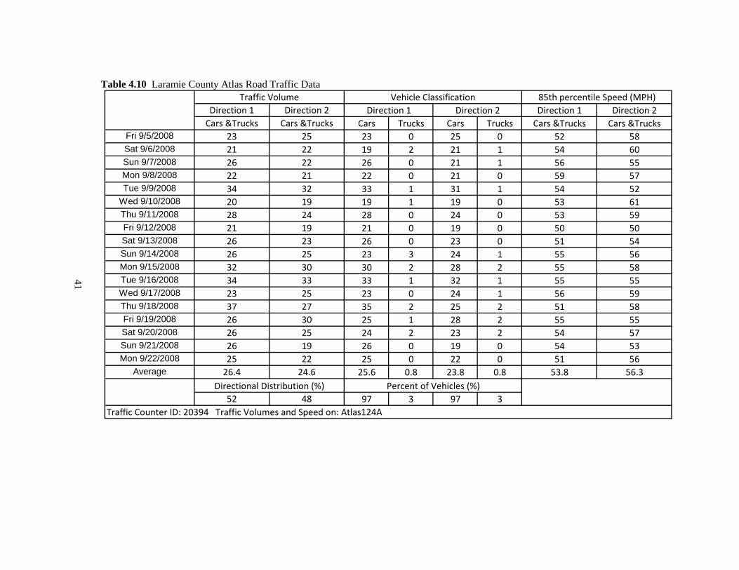
41

Table 4.10 Laramie County Atlas Road Traffic Data

Direction 1 Direction 2 Direction 1 Direction 2Cars &Trucks Cars &Trucks Cars Trucks Cars Trucks Cars &Trucks Cars &Trucks

Fri 9/5/2008 23 25 23 0 25 0 52 58Sat 9/6/2008 21 22 19 2 21 1 54 60Sun 9/7/2008 26 22 26 0 21 1 56 55Mon 9/8/2008 22 21 22 0 21 0 59 57Tue 9/9/2008 34 32 33 1 31 1 54 52

Wed 9/10/2008 20 19 19 1 19 0 53 61Thu 9/11/2008 28 24 28 0 24 0 53 59Fri 9/12/2008 21 19 21 0 19 0 50 50Sat 9/13/2008 26 23 26 0 23 0 51 54Sun 9/14/2008 26 25 23 3 24 1 55 56Mon 9/15/2008 32 30 30 2 28 2 55 58Tue 9/16/2008 34 33 33 1 32 1 55 55Wed 9/17/2008 23 25 23 0 24 1 56 59Thu 9/18/2008 37 27 35 2 25 2 51 58Fri 9/19/2008 26 30 25 1 28 2 55 55Sat 9/20/2008 26 25 24 2 23 2 54 57Sun 9/21/2008 26 19 26 0 19 0 54 53Mon 9/22/2008 25 22 25 0 22 0 51 56

Average 26.4 24.6 25.6 0.8 23.8 0.8 53.8 56.3

52 48 97 3 97 3Directional Distribution (%) Percent of Vehicles (%)

Traffic Counter ID: 20394 Traffic Volumes and Speed on: Atlas124A

Traffic Volume Vehicle Classification 85th percentile Speed (MPH)Direction 1 Direction 2

Table 4.11 Laramie County Pry Road Traffic Data

Direction 1 Direction 2 Direction 1 Direction 2Cars &Trucks Cars &Trucks Cars Trucks Cars Trucks Cars &Trucks Cars &Trucks

Fri 9/5/2008 25 42 23 2 20 22 55 47Sat 9/6/2008 21 16 19 2 15 1 61 57Sun 9/7/2008 16 13 16 0 13 0 56 61Mon 9/8/2008 24 19 22 2 18 1 55 54Tue 9/9/2008 31 19 30 1 19 0 59 51

Wed 9/10/2008 35 51 31 4 34 17 55 55Thu 9/11/2008 32 44 32 0 31 13 56 58Fri 9/12/2008 21 15 21 0 15 0 55 56Sat 9/13/2008 21 17 20 1 17 0 53 54Sun 9/14/2008 27 16 27 0 16 0 57 58Mon 9/15/2008 27 24 26 1 24 0 57 56Tue 9/16/2008 28 23 26 2 22 1 58 54Wed 9/17/2008 24 19 21 3 17 2 59 58

Average 25.5 24.5 24.1 1.4 20.1 4.4 56.6 55.3

51 49 94.5 5.5 82 18

Direction 2

Directional Distribution (%) Percent of Vehicles (%)

Traffic Counter ID: 20099 Traffic Volumes and Speed on: Pry224

Traffic Volume Vehicle Classification 85th percentile Speed (MPH)Direction 1

42

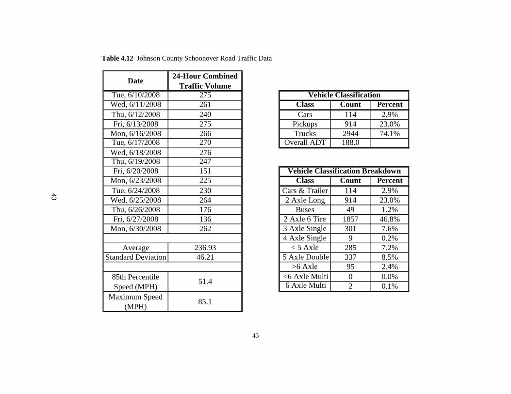
43

Table 4.12 Johnson County Schoonover Road Traffic Data

Tue, 6/10/2008 275Wed, 6/11/2008 261 Class Count PercentThu, 6/12/2008 240 Cars 114 2.9%Fri, 6/13/2008 275 Pickups 914 23.0%

Mon, 6/16/2008 266 Trucks 2944 74.1%Tue, 6/17/2008 270 Overall ADT 188.0Wed, 6/18/2008 276Thu, 6/19/2008 247Fri, 6/20/2008 151

Mon, 6/23/2008 225 Class Count PercentTue, 6/24/2008 230 Cars & Trailer 114 2.9%Wed, 6/25/2008 264 2 Axle Long 914 23.0%Thu, 6/26/2008 176 Buses 49 1.2%Fri, 6/27/2008 136 2 Axle 6 Tire 1857 46.8%

Mon, 6/30/2008 262 3 Axle Single 301 7.6%4 Axle Single 9 0.2%

Average 236.93 < 5 Axle 285 7.2%Standard Deviation 46.21 5 Axle Double 337 8.5%

>6 Axle 95 2.4% <6 Axle Multi 0 0.0% 6 Axle Multi 2 0.1%

85th Percentile Speed (MPH)

Maximum Speed (MPH)

24-Hour Combined Traffic VolumeDate

Vehicle Classification

51.4

85.1

Vehicle Classification Breakdown

43

44

4.6 Section Summary In this section, the collected field data as well as the laboratory results were presented. Dust, moisture content, wind speed, and wind direction were collected on every test section. The URCI produced from surface distress surveys on each test section was used to evaluate the performance of the test sections throughout the testing period. None of the test sections in Laramie County were considered as failing. One test section in Johnson County, gravel with CaCl, was considered failing by the end of the 2008 summer due to a URCI below 50. Traffic data were also collected on the three roads used in this study. The volumes of traffic between the two counties were significantly different. Schoonover Road in Johnson County experienced much heavier traffic volumes than two roads in Laramie County and it saw 74% trucks.

Samples of the materials used in this research were tested by the WYDOT Materials Testing Laboratory to determine the material characteristics. It was found that the gravel used in Laramie County had much more material passing the #200 (0.075mm) sieve compared with the gravel used in Johnson County. This trend also held true for the RAP blends used in each county. In the following chapter, a statistical analysis on the collected data is presented

45

45

5. DATA ANALYSIS

5.1 Introduction Following the data collection described in the previous chapter, preliminary and statistical analyses were performed on the data. The preliminary analysis involved visually inspecting plots of data to identify relationships that may be present in the data. Dust data were plotted against age, moisture content, and wind speed to detect possible relationships among the variables. These preliminary analyses were performed to gain an understanding of the behavior of data.

Statistical software was used to analyze the collected data. This analysis used statements within the general linear model (GLM) procedures to contrast groups of data. Using the contrast values, it could be determined what group of data was dominating the contrast. This technique allowed for more than one section to be in a given group allowing for comparisons to be made on more than a one-to-one basis. The groupings included sections containing the following characteristics: Laramie County, Johnson County, RAP, no RAP, calcium chloride (CaCl), and no CaCl.

A second statistical analysis was performed where the data was broken down by county as the test sections in both counties were constructed using different techniques. This analysis involved a sectional analysis of the test sections where individual test sections were compared with each other on a one-to-one basis. The test sections were compared using dust, Unsurfaced Road Condition Index (URCI), and surface distress data. Attempts at creating a model for predicting dust loss based on the collected data were made. This chapter describes the preliminary and statistical analyses used to evaluate the collected data. The analyses performed used Microsoft Excel and SAS 9.2 for Windows. The SAS code and results can be found Appendix D.

A general cost comparison analysis was also performed. The goal of this analysis was to evaluate the costs of using RAP and other dust suppressants in gravel roads. Furthermore, this analysis was performed to give agencies an idea of the cost effectiveness of using RAP in gravel roads.

5.2 Preliminary Analysis Visual inspection of the collected data was performed to detect any relationships found in the data. Dust was plotted against age, moisture content, and wind speed to help understand the behavior of the data. The data was broken down by county and test section to perform this analysis.

5.2.1 Dust vs. Age One relationship that was desired to analyze data behavior was dust loss versus age. In general, as a test section aged the dust loss decreased. As more dust is lost, there is less dust available to be removed from the section. When all of the dust data from Johnson County is plotted against the age of the test sections, there is a general decline in dust loss with time. The same general decrease holds true for the Laramie County data. Figures 5.1 and 5.2 show the dust versus age plots for Johnson and Laramie Counties, respectively. The decrease in dust with age also holds true for all of the individual sections within the counties. The plots for the individual sections can be found in Appendix A. Although this relationship can be visually seen, further research will be needed to quantitatively define the relationship.

46

Figure 5.1 Johnson County Dust vs. Age

Figure 5.2 Laramie County Dust vs. Age

0.0

0.2

0.4

0.6

0.8

1.0

1.2

1.4

1.6

1.8

2.0

0 20 40 60 80 100 120

1 m

i. D

ust

Wt.

(g)

Age (Days)

Johnson County Dust Wt. vs Age

0.0

1.0

2.0

3.0

4.0

5.0

6.0

7.0

0 20 40 60 80 100 120

1 m

i. D

ust

Wei

ght (

g)

Age (Days)

Laramie County Dust Wt. vs Age

47

5.2.2 Dust vs Moisture Content The dust loss and moisture content relationship was also investigated. It was concluded that no particular relationship between dust loss and moisture content in the individual sections can be established. This is because dust data were not collected when the roadway surface was wet. This resulted in a small range of moisture contents in which dust was collected. Also, within the small range of moisture contents there are no big variations in the collected dust weights. These conclusions hold true for both Johnson and Laramie Counties. Figures 5.3 and 5.4 give examples of dust loss versus moisture content in Johnson and Laramie Counties, respectively. The rest of the plotted data for dust loss versus moisture content can be found in Appendix A.

Figure 5.3 Example from Johnson County Dust vs. Moisture Content

0.0

0.2

0.4

0.6

0.8

1.0

1.2

1.4

1.6

1.8

2.0

0.00 0.50 1.00 1.50 2.00 2.50

1 m

i. D

ust

Wt.

(g)

Moisture Content (%)

Section S2: Dust vs Moisture Content

48

Figure 5.4 Example from Laramie County Dust vs. Moisture Content

5.2.3 Dust vs Wind Speed The relationship between dust loss and wind speed was also desired. It was suggested from visual inspection that a general trend between dust loss and wind speed could be inferred. The higher the wind speed, the lower the collected dust weight. Examples of this can be seen in Figures 5.5 and 5.6 for Johnson and Laramie Counties, respectively. It should also be noted that the variability in the dust weights is most likely attributed to the wind direction with respect to the direction of travel. That is, a strong headwind would force more dust into the collection box while a strong tailwind would prevent dust from reaching the box. It is suggested that dust collection should not be performed in high winds in order to ensure fair sampling.

0.00

1.00

2.00

3.00

4.00

5.00

6.00

7.00

0.000 0.500 1.000 1.500 2.000 2.500 3.000 3.500 4.000

1 m

i. D

ust

Wt.

(g)

MC (%)

Section A1: Dust Wt. vs MC

49

Figure 5.5 Example from Johnson County Dust vs. Wind Speed

Figure 5.6 Example from Laramie County Dust vs Wind Speed

5.3 Statistical Contrast Analysis

0.0

0.2

0.4

0.6

0.8

1.0

1.2

1.4

1.6

1.8

2.0

0 2 4 6 8 10 12 14 16 18

1 mi.

Dust

Wt.

(g)

Wind Speed (mph)

Section S2: Dust vs Wind Speed

0

0.5

1

1.5

2

2.5

0 5 10 15 20 25

1 m

i. D

ust

Wt.

(g)

Wind Speed (mph)

Section P1: Dust Wt. vs Wind Speed

50

Statistical software was used to analyze the collected data. This analysis used statements within the general linear model (GLM) procedures to contrast groups of data. The contrast values were used to determine what group of data was dominating the contrast. This technique allowed for more than one section to be in a given group, allowing for comparison to be made on more than a one-to-one basis. The groupings included sections containing the following comparisons: Laramie versus Johnson County, RAP versus no RAP, and calcium chloride (CaCl) versus no CaCl.

Contrasts were made on the basis of dust and URCI. All eight sections in the study were used in this analysis. An alpha value of 0.10 was chosen due to the inherent variability of unpaved roads. P-values were measured against the 0.10 value to determine if the groups were significantly different from one another. P-values less than 0.10 were considered significantly different and conclusions could be drawn. A contrast with a p-value greater than 0.10 was said to have no proof of the groups being significantly different and the results would not be considered. All contrasts in this analysis were found to be significantly different, therefore conclusions could be made.

In this analysis, a wind factor was established to help describe the effect of the wind on sampling. The wind speed, wind direction, and the angle in which the wind blew with respect to the roadway were used to establish the wind factor. Each direction of wind was given a degree value based on where it fell on a circle. A circle was broken up into sixteen segments to help describe the wind direction. North was given a value of zero. Moving in the clockwise direction each segment was 22.5 degrees larger than the last. A summary of the wind direction degree values can be found in Figure 5.7.

Figure 5.7 Wind Direction and Degree Values

Atlas Road in Laramie County runs east and west. Pry Road in Laramie County runs north and south. Schoonover Road in Johnson County runs NNW and SSE. The angle of the wind direction perpendicular

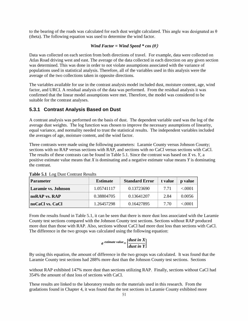
51

to the bearing of the roads was calculated for each dust weight calculated. This angle was designated as θ (theta). The following equation was used to determine the wind factor.

Wind Factor = Wind Speed * cos (θ)

Data was collected on each section from both directions of travel. For example, data were collected on Atlas Road driving west and east. The average of the data collected in each direction on any given section was determined. This was done in order to not violate assumptions associated with the variance of populations used in statistical analysis. Therefore, all of the variables used in this analysis were the average of the two collections taken in opposite directions.

The variables available for use in the contrast analysis model included dust, moisture content, age, wind factor, and URCI. A residual analysis of the data was performed. From the residual analysis it was confirmed that the linear model assumptions were met. Therefore, the model was considered to be suitable for the contrast analyses.

5.3.1 Contrast Analysis Based on Dust A contrast analysis was performed on the basis of dust. The dependent variable used was the log of the average dust weights. The log function was chosen to improve the necessary assumptions of linearity, equal variance, and normality needed to trust the statistical results. The independent variables included the averages of age, moisture content, and the wind factor.

Three contrasts were made using the following parameters: Laramie County versus Johnson County; sections with no RAP versus sections with RAP, and sections with no CaCl versus sections with CaCl. The results of these contrasts can be found in Table 5.1. Since the contrast was based on X vs. Y, a positive estimate value means that X is dominating and a negative estimate value means Y is dominating the contrast.

Table 5.1 Log Dust Contrast Results Parameter Estimate Standard Error t value p value

Laramie vs. Johnson 1.05741117 0.13723690 7.71 <.0001

noRAP vs. RAP 0.38804705 0.13641207 2.84 0.0056

noCaCl vs. CaCl 1.26457298 0.16427895 7.70 <.0001 From the results found in Table 5.1, it can be seen that there is more dust loss associated with the Laramie County test sections compared with the Johnson County test sections. Sections without RAP produced more dust than those with RAP. Also, sections without CaCl had more dust loss than sections with CaCl. The difference in the two groups was calculated using the following equation:

e estimate value= �dust in Xdust in Y

�

By using this equation, the amount of difference in the two groups was calculated. It was found that the Laramie County test sections had 288% more dust than the Johnson County test sections. Sections without RAP exhibited 147% more dust than sections utilizing RAP. Finally, sections without CaCl had 354% the amount of dust loss of sections with CaCl.

These results are linked to the laboratory results on the materials used in this research. From the gradations found in Chapter 4, it was found that the test sections in Laramie County exhibited more

52

material passing the #200 sieve than the Johnson County test sections. The gravel and RAP blend used in Laramie County had 23% and 2.2% material passing the #200 (0.075mm) sieve, respectively. In Johnson County, 11.6% of the gravel material and 1.0% of the RAP blend material passed the #200 (0.075mm) sieve. Therefore, more dust was available to be captured in Laramie County. Also, the roadways in the Laramie County were not compacted using a drum roller as they were in Johnson County.

The percentage of RAP blended material passing the #200 (0.075mm) sieve in Laramie County was 20% less than the percentage of gravel material passing the #200 (0.075mm) sieve. In Johnson County, the RAP blend had 10% less material passing the #200 (0.075mm) sieve than gravel. Therefore, any test sections that contained RAP would have less material available for capture as dust. Finally, the use of CaCl significantly reduced the amount of dust loss. This was expected as it is the nature of CaCl to capture moisture from the air surrounding the roadway surface and keep dust size materials from becoming airborne.

5.3.2 Contrast Analysis Based on URCI A contrast analysis was performed on the basis of the URCI. The dependent variable used was URCI, with dust, age, moisture content, and wind factor being the independent variables. Three contrasts were made using the following parameters: Laramie County versus Johnson County, sections with no RAP versus sections with RAP, and sections with no CaCl versus sections with CaCl. The results of these contrasts can be found in Table 5.2. Since the contrast was based on X vs. Y, a positive estimate value means that X is dominating and a negative estimate value means Y is dominating the contrast. The resulting contrast values only indicate which group is dominating the contrast and quantitative comparisons of the two values cannot be adequately developed due to the nature of the URCI being composed of multiple factors that are not necessarily the same in each group.

Table 5.2 URCI Contrast Results

Parameter Estimate Standard Error t Value p value

Laramie vs. Johnson 5.26596165 1.28732118 4.09 0.0001

noRAP vs. RAP 4.80737817 1.18336694 4.06 0.0001

noCaCl vs. CaCl 8.67047145 1.60173674 5.41 <.0001 Based the results found in Table 5.2, it can be seen that the URCI of the Laramie County test sections had better URCI scores compared with the Johnson County test sections. This is most likely due to a couple of factors. First, the volume of traffic on the Johnson County test sections (237 vpd) was much heavier than the traffic in Laramie County (25 vpd). Also, the number of trucks using the Johnson County test sections (74% trucks) was much more than the trucks using the Laramie County test sections (3-12% trucks). Secondly, CaCl was used on the Johnson County test sections. This presented the opportunity for rutting to occur on the sections with CaCl.

Sections without RAP had better URCI scores compared with sections with RAP. This is most likely due to the RAP sections having more loose aggregate. The amounts of loose aggregate on the RAP sections can be found in the URCI data sheets in Appendix B. This is further described in the following subsections that utilize sectional analysis methods. Sections without CaCl had better URCI scores than sections with CaCl. This is mainly due to the presence of rutting in the CaCl, which is described in more detail in the sectional analysis results in the following subsections.

5.4 Sectional Analysis of the Laramie County Test Sections

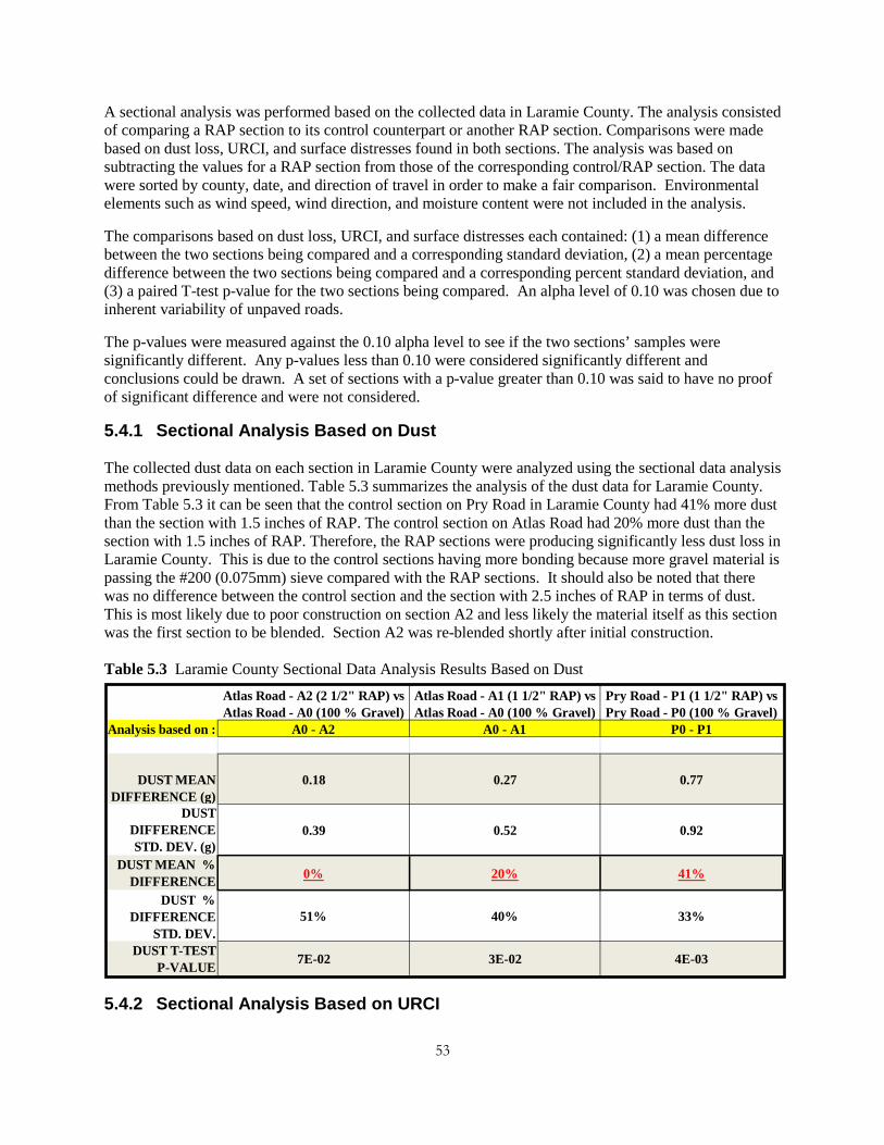
53

A sectional analysis was performed based on the collected data in Laramie County. The analysis consisted of comparing a RAP section to its control counterpart or another RAP section. Comparisons were made based on dust loss, URCI, and surface distresses found in both sections. The analysis was based on subtracting the values for a RAP section from those of the corresponding control/RAP section. The data were sorted by county, date, and direction of travel in order to make a fair comparison. Environmental elements such as wind speed, wind direction, and moisture content were not included in the analysis.

The comparisons based on dust loss, URCI, and surface distresses each contained: (1) a mean difference between the two sections being compared and a corresponding standard deviation, (2) a mean percentage difference between the two sections being compared and a corresponding percent standard deviation, and (3) a paired T-test p-value for the two sections being compared. An alpha level of 0.10 was chosen due to inherent variability of unpaved roads.

The p-values were measured against the 0.10 alpha level to see if the two sections’ samples were significantly different. Any p-values less than 0.10 were considered significantly different and conclusions could be drawn. A set of sections with a p-value greater than 0.10 was said to have no proof of significant difference and were not considered.

5.4.1 Sectional Analysis Based on Dust The collected dust data on each section in Laramie County were analyzed using the sectional data analysis methods previously mentioned. Table 5.3 summarizes the analysis of the dust data for Laramie County. From Table 5.3 it can be seen that the control section on Pry Road in Laramie County had 41% more dust than the section with 1.5 inches of RAP. The control section on Atlas Road had 20% more dust than the section with 1.5 inches of RAP. Therefore, the RAP sections were producing significantly less dust loss in Laramie County. This is due to the control sections having more bonding because more gravel material is passing the #200 (0.075mm) sieve compared with the RAP sections. It should also be noted that there was no difference between the control section and the section with 2.5 inches of RAP in terms of dust. This is most likely due to poor construction on section A2 and less likely the material itself as this section was the first section to be blended. Section A2 was re-blended shortly after initial construction. Table 5.3 Laramie County Sectional Data Analysis Results Based on Dust

5.4.2 Sectional Analysis Based on URCI

Analysis based on : A0 - A2 A0 - A1 P0 - P1

DUST MEAN DIFFERENCE (g)

0.18 0.27 0.77

DUST DIFFERENCE STD. DEV. (g)

0.39 0.52 0.92

DUST MEAN % DIFFERENCE 0% 20% 41%

DUST % DIFFERENCE

STD. DEV.51% 40% 33%

DUST T-TEST P-VALUE 7E-02 3E-02 4E-03

Atlas Road - A2 (2 1/2" RAP) vs Atlas Road - A0 (100 % Gravel)

Atlas Road - A1 (1 1/2" RAP) vs Atlas Road - A0 (100 % Gravel)

Pry Road - P1 (1 1/2" RAP) vs Pry Road - P0 (100 % Gravel)

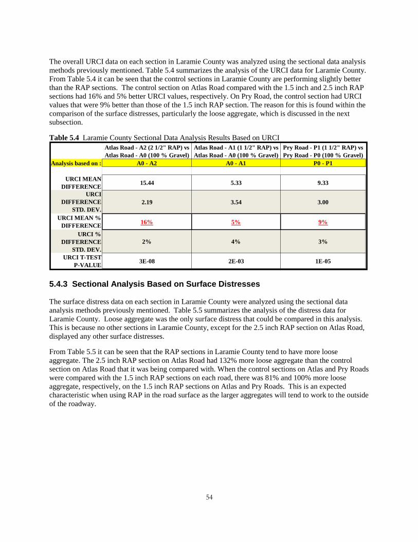
54

The overall URCI data on each section in Laramie County was analyzed using the sectional data analysis methods previously mentioned. Table 5.4 summarizes the analysis of the URCI data for Laramie County. From Table 5.4 it can be seen that the control sections in Laramie County are performing slightly better than the RAP sections. The control section on Atlas Road compared with the 1.5 inch and 2.5 inch RAP sections had 16% and 5% better URCI values, respectively. On Pry Road, the control section had URCI values that were 9% better than those of the 1.5 inch RAP section. The reason for this is found within the comparison of the surface distresses, particularly the loose aggregate, which is discussed in the next subsection.

Table 5.4 Laramie County Sectional Data Analysis Results Based on URCI

5.4.3 Sectional Analysis Based on Surface Distresses The surface distress data on each section in Laramie County were analyzed using the sectional data analysis methods previously mentioned. Table 5.5 summarizes the analysis of the distress data for Laramie County. Loose aggregate was the only surface distress that could be compared in this analysis. This is because no other sections in Laramie County, except for the 2.5 inch RAP section on Atlas Road, displayed any other surface distresses.

From Table 5.5 it can be seen that the RAP sections in Laramie County tend to have more loose aggregate. The 2.5 inch RAP section on Atlas Road had 132% more loose aggregate than the control section on Atlas Road that it was being compared with. When the control sections on Atlas and Pry Roads were compared with the 1.5 inch RAP sections on each road, there was 81% and 100% more loose aggregate, respectively, on the 1.5 inch RAP sections on Atlas and Pry Roads. This is an expected characteristic when using RAP in the road surface as the larger aggregates will tend to work to the outside of the roadway.

Analysis based on : A0 - A2 A0 - A1 P0 - P1

URCI MEAN DIFFERENCE 15.44 5.33 9.33

URCI DIFFERENCE

STD. DEV.2.19 3.54 3.00

URCI MEAN % DIFFERENCE 16% 5% 9%

URCI % DIFFERENCE

STD. DEV.2% 4% 3%

URCI T-TEST P-VALUE 3E-08 2E-03 1E-05

Pry Road - P1 (1 1/2" RAP) vs Pry Road - P0 (100 % Gravel)

Atlas Road - A2 (2 1/2" RAP) vs Atlas Road - A0 (100 % Gravel)

Atlas Road - A1 (1 1/2" RAP) vs Atlas Road - A0 (100 % Gravel)

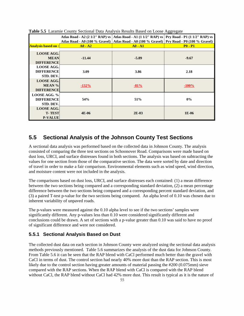
55

Table 5.5 Laramie County Sectional Data Analysis Results Based on Loose Aggregate

5.5 Sectional Analysis of the Johnson County Test Sections A sectional data analysis was performed based on the collected data in Johnson County. The analysis consisted of comparing the three test sections on Schoonover Road. Comparisons were made based on dust loss, URCI, and surface distresses found in both sections. The analysis was based on subtracting the values for one section from those of the comparative section. The data were sorted by date and direction of travel in order to make a fair comparison. Environmental elements such as wind speed, wind direction, and moisture content were not included in the analysis.

The comparisons based on dust loss, URCI, and surface distresses each contained: (1) a mean difference between the two sections being compared and a corresponding standard deviation, (2) a mean percentage difference between the two sections being compared and a corresponding percent standard deviation, and (3) a paired T-test p-value for the two sections being compared. An alpha level of 0.10 was chosen due to inherent variability of unpaved roads.

The p-values were measured against the 0.10 alpha level to see if the two sections’ samples were significantly different. Any p-values less than 0.10 were considered significantly different and conclusions could be drawn. A set of sections with a p-value greater than 0.10 was said to have no proof of significant difference and were not considered.

5.5.1 Sectional Analysis Based on Dust The collected dust data on each section in Johnson County were analyzed using the sectional data analysis methods previously mentioned. Table 5.6 summarizes the analysis of the dust data for Johnson County. From Table 5.6 it can be seen that the RAP blend with CaCl performed much better than the gravel with CaCl in terms of dust. The control section had nearly 40% more dust than the RAP section. This is most likely due to the control section having greater amounts of material passing the #200 (0.075mm) sieve compared with the RAP sections. When the RAP blend with CaCl is compared with the RAP blend without CaCl, the RAP blend without CaCl had 42% more dust. This result is typical as it is the nature of

Analysis based on : A0 - A2 A0 - A1 P0 - P1

LOOSE AGG. MEAN

DIFFERENCE-11.44 -5.89 -9.67

LOOSE AGG. DIFFERENCE

STD. DEV.3.09 3.86 2.18

LOOSE AGG. MEAN %

DIFFERENCE-132% -81% -100%

LOOSE AGG. % DIFFERENCE

STD. DEV.54% 51% 0%

LOOSE AGG. T- TEST

P-VALUE4E-06 2E-03 1E-06

Atlas Road - A2 (2 1/2" RAP) vs Atlas Road - A0 (100 % Gravel)

Atlas Road - A1 (1 1/2" RAP) vs Atlas Road - A0 (100 % Gravel)

Pry Road - P1 (1 1/2" RAP) vs Pry Road - P0 (100 % Gravel)

56

roadways with CaCl to exhibit less dust loss than those without CaCl. Results could not be drawn from the RAP blend compared with the gravel with CaCl because the p-value of 0.70 is greater than the alpha value of 0.10, which suggests that the two sections are not significantly different in terms of dust.

Table 5.6 Johnson County Sectional Data Analysis Results Based on Dust

5.5.2 Sectional Analysis Based on URCI The overall URCI data on each section in Johnson County were analyzed using the sectional data analysis methods previously mentioned. Table 5.7 summarizes the analysis of the URCI data for Johnson County. From Table 5.7 it can be seen that there was no significant difference in the Johnson County sections in terms of URCI due to the p-values being greater than 0.10. But there are specific findings for individual distresses as seen in the next subsection.

Table 5.7 Johnson County Sectional Data Analysis Results Based on URCI

Analysis based on : S0 - S1 S0 - S2 S2 - S1

DUST MEAN DIFFERENCE (g) 0.35 0.07 0.28

DUST DIFFERENCE STD. DEV. (g) 0.42 0.51 0.26

DUST MEAN % DIFFERENCE 40% -50% 42%

DUST % DIFFERENCE STD. DEV. 33% 124% 32%

DUST T-TEST P-VALUE 3E-02 7E-01 7E-05

S1 (RAP Blend w/ CaCl) vs S0 (Gravel w/ CaCl)

S2 (RAP Blend) vs S0 (Gravel w/ CaCl)

S1 (RAP Blend w/ CaCl) vs S2 (RAP Blend)

Analysis based on : S0 - S1 S0 - S2 S2 - S1

URCI MEAN DIFFERENCE -4.83 -6.67 1.83

URCI DIFFERENCE STD. DEV. 8.98 8.82 4.26

URCI MEAN % DIFFERENCE -7% -9% 2%

URCI % DIFFERENCE STD. DEV.

14% 14% 5%

URCI T-TEST P-VALUE 2E-01 1.2E-01 3E-01

S1 (RAP Blend w/ CaCl) vs S2 (RAP Blend)

S1 (RAP Blend w/ CaCl) vs S0 (Gravel w/ CaCl)

S2 (RAP Blend) vs S0 (Gravel w/ CaCl)

57

5.5.3 Sectional Analysis Based on Surface Distresses The surface distress data on each section in Johnson County was analyzed using the sectional data analysis methods previously mentioned. Table 5.8 summarizes the analysis of the distress data for Johnson County. From Table 5.8 it can be seen that rutting and loose aggregate had significant findings. The S0-S2 set has no viable comparison for loose aggregate due to a p-value greater than 0.10. The gravel with CaCl section showed almost 26% more loose aggregate than the RAP blend with CaCl section. The RAP blend section also showed 39.5% more loose aggregate than the RAP blend with CaCl section. In terms of rutting, the RAP blend with CaCl showed 67% more rutting than the RAP blend by itself. The gravel with CaCl showed 83% more rutting than the RAP blend without CaCl. This is not surprising due to the nature of CaCl and its effect on the moisture content of the road surface.

Table 5.8 Johnson County Sectional Data Analysis Results Based on Surface Distresses

Analysis based on : S0 - S1 S0 - S2 S2 - S1LOOSE AGG. MEAN

DIFFERENCE 2.50 -0.67 3.17

LOOSE AGG. DIFFERENCE STD. 2.26 3.14 2.48

LOOSE AGG. MEAN % DIFFERENCE 26% -12% 39%

LOOSE AGG. % DIFFERENCE STD. 27% 44% 38%

LOOSE AGG. T-TEST P-VALUE 4E-02 6E-01 3E-02

RUT MEAN DIFFERENCE 3.00 9.67 -6.67

RUT DIFFERENCE STD. DEV. 8.65 10.21 5.50

RUT MEAN % DIFFERENCE 18% 83% -67%

RUT % DIFFERENCE STD. 56% 41% 52%

RUT T-TEST P-VALUE 4E-01 7E-02 3E-02

S1 (RAP Blend w/ CaCl) vs S0 (Gravel w/ CaCl)

S2 (RAP Blend) vs S0 (Gravel w/ CaCl)

S1 (RAP Blend w/ CaCl) vs S2 (RAP Blend)

58

5.6 Cost Comparison Analysis A general cost analysis was performed to evaluate the cost effectiveness of utilizing RAP in gravel roads. This analysis only takes into account material costs and does not account for construction, maintenance, labor, or user cost. It is suggested that these costs should be collected for Phase II of this project in order to adequately develop a benefit-cost analysis.

The main component of a gravel road is the aggregate. The 2009 WYDOT weighted average price for crusher run aggregate was $6.90/ton. A density of 150 pcf was assumed for the crusher run aggregate. Additional cost on a gravel road is the cost of dust suppressants. For this analysis, Magnesium Chloride (MgCl) was used as this product will be utilized in Phase II of this project. As quoted by the Desert Mountain Corporation, the cost to deliver and apply MgCl is $0.53/gallon with an application rate of 0.5 gallons/yd2. Also, the 2009 WYDOT weighted average price for RAP was $12.77/yd3. A density value of 140 pcf was assumed for the RAP. Therefore, the cost of RAP was calculated to be $6.75/ton.

The basic design of Phase II of this project has developed one-mile test sections that will consist of 6 inches of RAP or aggregate blended with three inches of native soils. The width of the roadway is 27 feet. This data were utilized to perform the cost comparison. The comparison made was between the material cost of a one-mile RAP blended section and a one-mile section of crusher run aggregate with MgCl.

To cover a roadway that is 27 feet wide with 6 inches of material for one mile will take 71,280 feet3 of material. It would take 4,990 tons of RAP or 5,346 tons of crusher run aggregate to cover the one-mile roadway at a depth of 6 inches. Therefore, the material cost for the RAP is $33,683.50. The material cost for the aggregate is $36,887.40. A one-mile long road that is 27 feet wide has 142,560 square yards in it. A total of 71,280 gallons of MgCl would be needed to cover the road at a delivery and application cost of $37,778.40. Therefore, the total cost for the RAP section is $33,683.50, and the total cost of the aggregate with the MgCl section is $74,665.80. If MgCl was added to the RAP section, the total cost would be $71,460.90.

In terms of cost effectiveness, this general materials cost comparison shows that RAP is a cost effective material for use in gravel roads; and, as prior analyses show, RAP blends reduce dust loss. These are only general comparisons, and it is suggested for Phase II of this project to confirm this analysis. Initial construction and material costs need to collected. Application costs associated with dust suppressants as well as long-term maintenance costs will also be needed to perform the actual cost analysis.

5.7 Section Summary Multiple analyses were performed on the collected data from the test sections. These analyses included a preliminary analysis where visual inspection of the collected data was performed to detect any relationships found in the data. Dust was plotted against age, moisture content, and wind speed to help understand the behavior of the data.

From the preliminary analysis it appears that dust loss decreased with age. When dust loss was compared with moisture content, it was implied that moisture content did not have any effect on dust loss at low moisture contents. It was implied from the dust loss and wind speed comparison that dust measurements were affected by wind speed, and collection should not be attempted during high winds in order to ensure fair data collection.

59

A contrast analysis was also performed on the collected data. In this analysis, groups of data were compared with one another. Contrasts were made on the basis of dust loss as well as URCI. Three contrasts for dust loss and three contrasts for URCI were made using the following parameters: Laramie County versus Johnson County, sections with no RAP versus sections with RAP, and sections with no CaCl versus sections with CaCl.

The contrast analysis based on dust found that the Laramie County test sections had 288% more dust than the Johnson County test sections. Sections without RAP produced 147% more dust than those with RAP. Test sections without CaCl exhibited 354% more dust than sections with CaCl. The reason for these large differences in dust can be found in the materials used within each section with particular emphasis on the percentage of material passing the #200 sieve.

The contrast analysis based on URCI values found that the Laramie County test sections had higher URCI scores compared with the Johnson County test sections. Sections without RAP were found to have higher scores than those with RAP, mostly due to larger amounts of loose aggregate on the RAP sections. Test sections without CaCl were found to have higher URCI scores than sections with CaCl due to the rutting present in the sections utilizing CaCl.

Finally, a sectional statistical analysis was performed on the collected data from the test sections. The purpose of this analysis was to compare the test sections within a given county based on dust, URCI, and surface distresses. The analysis was based on subtracting the values for a RAP section from those of the comparative section.

The sectional analysis performed on the dust data found that the RAP sections in Laramie County had significantly less dust loss than the control sections. In Johnson County, the RAP blend with CaCl performed much better than the gravel with CaCl in terms of dust. When CaCl was not used with the RAP blend section, the gravel with CaCl had less dust loss. When the RAP blend with CaCl was compared with the RAP blend without CaCl, the RAP blend without CaCl created 42% more dust.

The sectional analysis performed on the basis of URCI found that the gravel control sections in Laramie County performed slightly better than the RAP sections. The result from the analysis performed on the Johnson County URCI data revealed no significant difference in the three sections on Schoonover Road. This was due to the resulting p-values being larger than the set value of 0.10.

The sectional analysis performed on the surface distress found that the RAP sections in Laramie County experienced more loose aggregate than the RAP sections. In Johnson County, the RAP blend with CaCl had the least amount of loose aggregate followed by gravel with CaCl. The RAP blend without CaCl had the most loose aggregate. In terms of rutting, the sections with CaCl showed more rutting. The gravel with CaCl exhibited the worst rutting of the three sections.

A general cost analysis showed that RAP is a cost effective material for use in gravel roads. It is suggested that Phase II of this project collect construction and maintenance cost data in order to perform a thorough cost analysis of the actual test sections and confirm that RAP is a cost effective material in gravel roads.

60

61

6. CONCLUSIONS AND RECOMMENDATIONS 6.1 Summary This research project utilized field and laboratory evaluations to study the performance of using Recycled Asphalt Pavement (RAP) in gravel roads by focusing on its ability to reduce dust loss and maintain roadway stability. The field evaluations involved observing eight test sections constructed in two Wyoming counties. Dust collection was accomplished using the Colorado State University Dustometer. Surface distresses were monitored following methods developed by the United States Army Corps of Engineers. Conditions related to wind were collected using a handheld wind vane and digital compass. Roadway moisture content was determined from surface samples. Laboratory evaluations involved material testing performed by WYDOT. All of this data were collected in a database to allow for statistical analyses to be performed in order to evaluate the effectiveness of RAP in gravel roads.

6.2 Conclusions From the preliminary analysis of the collected data it was observed that dust loss decreased with age. It was also concluded that dust collection should not be taken when wind speeds are high. Dust measurements were taken when the roadway was dry and the moisture content was low. Therefore, at low moisture contents it was determined that moisture content did not appear to affect dust loss.

From the contrast analysis based on dust, sections without RAP generated 147% more dust loss than sections with RAP. The asphalt within the RAP provided better binding for the materials. Test sections without CaCl generated 354% more dust than sections with CaCl. The amount of dust loss in the Laramie County test sections was greater than those in Johnson County by 288% because the materials used in Laramie County had significantly higher percentages of material passing the #200 (0.075mm) sieve.

From the contrast analysis based on URCI, the URCI values in Laramie County were better than the URCI values in Johnson County due to the differences in traffic volumes, particularly when comparing truck traffic (3-12% versus 74% trucks). Sections without RAP had URCI values that were better than sections with RAP due to larger amounts of loose aggregate associated with RAP sections. Sections without CaCl had URCI values that were better than sections with CaCl due to the rutting associated with the use of CaCl. Conclusions drawn from sectional analyses of the data are broken down by county and found in the following two subsections.

From the general cost analysis it was observed that RAP is a cost effective material for use in gravel roads. It is suggested that Phase II of this project collect construction and maintenance cost data in order to perform a thorough cost analysis of the actual test sections and confirm that RAP is a cost effective material in gravel roads.

6.2.1 Laramie County Conclusions Based on the observations and testing performed on the Laramie County test sections, the following conclusions were drawn:

1. The use of RAP in gravel roads reduced dust loss from 0 to 41%.

2. Overall road serviceability, based on the URCI, was slightly better for the 100% gravel sections. This was due to more loose aggregate seen on the RAP sections.

62

3. The sections with RAP exhibited significantly more amounts of loose aggregate than the 100% gravel sections.

4. The construction technique blending the RAP and gravel on site by means of a blade led to segregation of the material, resulting in large amount of loose aggregate.

5. Loose aggregate was the main surface distress that was apparent in the Laramie County test sections, especially in the RAP sections.

6. The overall conclusion was that RAP significantly reduced dust loss with no improvement in road condition.

6.2.1 Johnson County Conclusions Based on the observations and testing performed on the Johnson County test sections, the following conclusions were drawn:

1. The RAP blend section and the gravel with CaCl section were not significantly different in terms of dust, URCI, or loose aggregate.

2. There was no statistical significant difference in the URCI among the three test sections. That is, the RAP sections did not make any improvements in the overall serviceability of the roadway compared with the control section.

3. The gravel with CaCl section showed more loose aggregate than the RAP blend with CaCl section. The RAP blend section without CaCl displayed more loose aggregate than the RAP blend with CaCl. The use of CaCl helped in stabilizing the road surface and reducing the amount of loose aggregate.

4. The sections with CaCl had more rutting than the section without CaCl.

5. The use of RAP in the roadway reduced dust loss. RAP with CaCl reduced dust loss even more.

6. The overall conclusion was that RAP significantly reduced dust loss with no adverse effects to the road serviceability. In addition, using CaCl with the RAP blend further reduced dust loss.

6.3 Recommendations to Agencies This project thoroughly investigated the use of RAP in gravel roads in two Wyoming counties. From this investigation it has been concluded that the use of RAP is an effective tool for reducing dust loss without compromising road serviceability. For any agency that has a desire to reduce the amount of dust loss on their gravel roads, it is suggested that they follow these recommendations:

1. Blend RAP into the existing gravel road surface or blend RAP with virgin aggregate in a pugmill and place on the existing unsurfaced road to reduce dust loss. If applicable, RAP and gravel should be blended in a pugmill rather than in place to avoid segregation of materials from blade mixing.

2. Compact the RAP blend with a roller if at all possible. This will help in maintaining the long-term road serviceability.

63

3. Combine CaCl with the RAP blend to further reduce dust loss as well as reduce loose aggregate.

4. Attention should be directed to traffic volumes as there are trade-offs between using RAP and CaCl in gravel roads. Reduced dust loss is most likely more important than minor amounts of loose aggregate and rutting.

5. Attention should be directed to the initial gradations of the materials being used in order to help reduce loss and provide adequate binding. Materials with large amounts of fines (>15% passing the #200 [0.075 mm] sieve) will have more dust available to be lost.

6.4 Recommendations for Phase II 1. Additional field evaluations should be performed to determine the optimum design and

construction technique of incorporating RAP into gravel roads.

2. Dust measurements should not be performed on test sections when wind speeds are high and/or when the roadway is wet.

3. Further research should be performed to quantitatively describe the effects of the wind on dust loss. This should be done by developing laboratory techniques to analyze the relationship between dust and wind

4. Laboratory tests should be developed to help correlate field data to lab data. The test(s) should simulate field data in order to make sound statistical analyses. Once verified, the test(s) could be used to make conclusions about a material’s dust loss and serviceability.

5. Further research should be performed to study the effects of traffic, especially trucks, on the performance of gravel roads using RAP and other dust suppressants.

6. This research project has determined that RAP used in gravel roads reduces dust loss without adversely affecting road serviceability. Given the benefits that may be utilized by using RAP, further investigations into its use are justified.

7. Construction and maintenance cost data should be collected in order to perform a thorough cost analysis of the actual test sections and confirm that RAP is a cost effective material in gravel roads.

64

65

REFERENCES AASHTO Center for Environmental Excellence. (2003). Taking the High Road: The Environmental and Social Contributions of America's Highway Programs. Washington DC: American Association of State Highway and Transportation Officials.

Addo, J. Q., T.G. Sanders, and & M. Chenard. (2004). Road Dust Supression: Effect on Maintenance Stability, Safety and the Environment Phases 1-3. Colorado State University, Department of Civil Engineering. Ft. Collins, CO: Mountain Plains Consortium.

Cosentino, P., E. Kalajian, and C.-S. Shieh. (2003). Developing Specifications for Using Recycled Asphalt Pavement as Base, Subbase or General Fill Materials,Phase II Final Report. Florida Institute of Trechnology, Civil Engineering Department. Gainesville, FL: Florida Department of Transportation.

Davio, R. (1999). June: Reclaimed Asphalt Pavement. Year of the Recycled Roadway Materials (June) . Austin, TX: Texas Department of Transportation.

Desert Mountain Corporation (Riverton, WY). (2010, June 18). Dust Suppressant Price Quotation sent to the Wyoming Technology Transfer Center at the University of Wyoming. Laramie, WY.

Eaton, R. A., and R.E. Beaucham. (1992). Unsurfaced Road Maintenence Management Special Report 92-26. U.S. Army Corps of Engineers, Cold Regions Research & Engineering Labratory. Washington DC: U.S. Army Corps of Engineers.

FHWA. (1998). User Guidelines for Waste and By-Product Materials in Pavement Construction. Washington DC: Federal Highway Administration.

Hoover, J., K. Bergerso, D. Fox, C. Denny, and R. Handy. (1973). Surface Improvemnt and Dust Palliation of Unpaved Secondary Roads and Streets. Final Report H-194 Iowa Highway Research Board Project.

Huber, G. (2008). Recycled Asphalt Pavement: FHWA RAP Expert Task Group. Illinois Bituminous Paving Conference & North Central Asphalt User/Producer Group Conference. Springfield: Heritage Research Group.

Irwin, L., D. Taylor, and D. Aneshansley. (1986). Device to Measure Road Dustiness on Aggregate Surface Roads. Cornell Local Road Program Report 86.5, Dept. of Argicultural Engineering, Cornell University, Ithaca, NY.

Kuennen, T. (2006, August). “Control of Dust Is a Major Must.” Better Roads , 76 (8), pp. 20-29.

Langdon, B. (1984). Dust Volume Sampler Documentation. USDA Forest Service, Mount Hood National Forest.

Li, L., C.H. Benson, T.B. Edil, and B. Hatipoglu. (2007). Sustainable Construction Case History: Fly Ash Stabilization of Recycled Asphalt Pavement Material. Transportation Research Board 86th Annual Meeting. Washington DC: Transportation Research Board.

Monlux, S., and M.R. Mitchell. (2006). Surface-Aggregate Stabilization with Chloride Materials. Washington DC: U.S. Department of Agriculture: Forest Service .

66

Morgan, R.J., V. Schaefer, and R.S. Sharma. (2005). Determination and Evaluation of Alternative Methods for Managing and Controlling Highway-Related Dust. Iowa State University, Department of Civil, Construction and Environmental Engineering. Ames, IA: Iowa Highway Research Board.

Putnam, B.J., J. Aune, and S.N. Amirkhanian. (2002). Recycled Asphalt Pavement (RAP)Used in Superpave Mixes Made with Rubberized Asphalt. Clemson University, Asphalt Rubber Technology Service. Clemson: Clemson University.

Rathje, E.M., A.F. Rauch, D. Trejo, K.J. Folliard, C. Viyanant, M. Esfellar, et al. (2006). Evaluation of Crushed Concrete and Recycled Asphalt Pavement as Backfill for Mechanically Stabilized Earth Walls. The University Texas at Austin, Center for Transportation Research. Austin, TX: Texas Department of Transportation.

Sanders, T.G. and J.Q. Addo. (1993). Effectiveness and Environmental Impact of Road Dust Suppressants. Colorado State University, Department of Civil Engineering. Ft. Collins, CO: Mountain Plains Consortium.

Sanders, T.G. and J.Q. Addo. (2000). “Experimental Road Dust Measurement Device.” Journal of Transportation Engineers , 123 (No.6), 530-535.

Skorseth, K. and A.A. Selim. (2005). Gravel Roads: Maintenance and Design Manual. Federal Highway Administration, South Dakota Local Transportation Assistance Program. Washington DC: FHWA.

Sullivan, J. (1996). Pavement Recycling Executive Summary and Report. Federal Highway Administration, Office of Enineering and Office of Technology Applications. Washington DC: Federal Highway Administration.

Walker, D., L. Entine, and S. Kummer. (2002). Gravel Roads PASER Manual. University of Wisconsin-Madison, Transportation Information Center. Madison, WI: Wisconsin Transportation Information Center.

Wellman, E. and S. Barraclough. (1972). Establishment of Acceptable Dusting Criteria for Aggregate Surface Raods. Winema National Forest: Study 7110, USDA Forest Service Administration.

WYDOT. (2010, January 04). 2009 Weighted Average Bid Prices. Retrieved August 2010, from http://www.dot.state.wy.us/webdav/site/wydot/shared/Contracts%20and%20Estimates/2009%20English.pdf

67

APPENDIX A DUST COLLECTION, MOISTURE CONTENT, AND WIND DATA

68

1 Atlas Road - A2 (2 1/2" RAP) 6/9/2008 7:55 AM 20 W 1.82 2.0442 Atlas Road - A1 (1 1/2" RAP) 6/9/2008 8:10 AM 20 W 6.20 0.9913 Atlas Road - A0 (100% Gravel) 6/9/2008 8:25 AM 20 W 5.78 2.5914 Pry Road - P1 (1 1/2" RAP) 6/9/2008 8:30 AM 20 W 0.64 2.1055 Pry Road - P0 (100% Gravel) 6/9/2008 8:35 AM 20 W 0.38 2.5496 Atlas Road - A2 (2 1/2" RAP) 6/17/2008 7:25 AM 10 W 3.86 0.4777 Atlas Road - A1 (1 1/2" RAP) 6/17/2008 7:30 AM 10 W 6.52 0.6458 Atlas Road - A0 (100% Gravel) 6/17/2008 7:40 AM 10 W 3.76 1.0299 Pry Road - P1 (1 1/2" RAP) 6/17/2008 7:45 AM 10 W 0.88 0.767

10 Pry Road - P0 (100% Gravel) 6/17/2008 7:50 AM 10 W 0.92 1.31411 Atlas Road - A2 (2 1/2" RAP) 6/24/2008 7:10 AM 10 WNW 2.40 6.36212 Atlas Road - A1 (1 1/2" RAP) 6/24/2008 7:20 AM 10 WNW 1.58 3.38513 Atlas Road - A0 (100% Gravel) 6/24/2008 7:30 AM 10 WNW 2.40 5.04414 Pry Road - P1 (1 1/2" RAP) 6/24/2008 7:35 AM 10 WNW 2.34 4.93615 Pry Road - P0 (100% Gravel) 6/24/2008 7:40 AM 10 WNW 5.84 5.52316 Atlas Road - A2 (2 1/2" RAP) 7/11/2008 7:40 AM 15 W 2.20 0.73617 Atlas Road - A2 (2 1/2" RAP) 7/28/2008 8:45 AM 16 WNW 0.76 0.66218 Atlas Road - A1 (1 1/2" RAP) 7/28/2008 8:40 AM 20 W 0.42 0.77719 Atlas Road - A0 (100% Gravel) 7/28/2008 8:30 AM 20 WNW 0.96 1.19320 Pry Road - P1 (1 1/2" RAP) 7/28/2008 9:15 AM 11 WNW 0.64 0.60521 Pry Road - P0 (100% Gravel) 7/28/2008 9:05 AM 12 WNW 1.08 1.18522 Atlas Road - A2 (2 1/2" RAP) 7/28/2008 7:30 AM 11 W 0.20 0.66223 Atlas Road - A1 (1 1/2" RAP) 7/28/2008 7:50 AM 10 W 0.14 0.77724 Atlas Road - A0 (100% Gravel) 7/28/2008 8:10 AM 17 WNW 0.08 1.19325 Pry Road - P1 (1 1/2" RAP) 7/28/2008 9:30 AM 13 WNW 0.24 0.60526 Pry Road - P0 (100% Gravel) 7/28/2008 9:35 AM 14 WNW 0.36 1.18527 Atlas Road - A2 (2 1/2" RAP) 7/29/2008 3:50 PM 5 W 0.66 0.39928 Atlas Road - A1 (1 1/2" RAP) 7/29/2008 4:00 PM 7 W 0.80 0.23929 Atlas Road - A0 (100% Gravel) 7/29/2008 4:15 PM 6 W 0.74 0.73230 Pry Road - P1 (1 1/2" RAP) 7/29/2008 4:25 PM 10 W 0.54 0.31631 Pry Road - P0 (100% Gravel) 7/29/2008 4:35 PM 8 W 1.52 0.59432 Atlas Road - A2 (2 1/2" RAP) 7/29/2008 4:55 PM 10 W 1.60 0.39933 Atlas Road - A1 (1 1/2" RAP) 7/29/2008 4:50 PM 8 W 1.24 0.23934 Atlas Road - A0 (100% Gravel) 7/29/2008 4:45 PM 12 W 2.50 0.73235 Pry Road - P1 (1 1/2" RAP) 7/29/2008 4:40 PM 11 W 0.84 0.31636 Pry Road - P0 (100% Gravel) 7/29/2008 4:30 PM 9 W 1.80 0.59437 Atlas Road - A2 (2 1/2" RAP) 8/6/2008 8:00 AM 10 WNW 0.18 0.45738 Atlas Road - A1 (1 1/2" RAP) 8/6/2008 8:10 AM 14 WNW 0.10 0.50039 Atlas Road - A0 (100% Gravel) 8/6/2008 8:15 AM 15 NW 0.16 0.89240 Pry Road - P1 (1 1/2" RAP) 8/6/2008 8:20 AM 16 NW 0.52 0.69641 Pry Road - P0 (100% Gravel) 8/6/2008 8:30 AM 10 NW 1.98 0.84542 Atlas Road - A2 (2 1/2" RAP) 8/6/2008 7:55 AM 12 NW 0.48 0.45743 Atlas Road - A1 (1 1/2" RAP) 8/6/2008 7:45 AM 16 NW 0.70 0.50044 Atlas Road - A0 (100% Gravel) 8/6/2008 7:35 AM 15 NW 0.56 0.89245 Pry Road - P1 (1 1/2" RAP) 8/6/2008 8:45 AM 11 NW 0.30 0.696

Laramie County Dust, Moisture, and Wind Data

# Test Section Date of Sample

Time of Sample Wind (mph) 1 mi. Dust

Wt. (g)Moisture

Content (%)

69

46 Pry Road - P0 (100% Gravel) 8/6/2008 8:40 AM 9 NW 1.26 0.84547 Atlas Road - A2 (2 1/2" RAP) 8/7/2008 3:00 PM 11 S 0.40 0.42548 Atlas Road - A1 (1 1/2" RAP) 8/7/2008 3:10 PM 10 S 0.44 0.37749 Atlas Road - A0 (100% Gravel) 8/7/2008 3:25 PM 7 SE 0.70 0.72250 Pry Road - P1 (1 1/2" RAP) 8/7/2008 3:30 PM 8 SE 0.36 0.29151 Pry Road - P0 (100% Gravel) 8/7/2008 3:40 PM 10 S 0.62 0.59952 Atlas Road - A2 (2 1/2" RAP) 8/7/2008 4:05 PM 8 S 0.34 0.42553 Atlas Road - A1 (1 1/2" RAP) 8/7/2008 4:00 PM 9 S 0.10 0.37754 Atlas Road - A0 (100% Gravel) 8/7/2008 3:55 PM 9 S 0.18 0.72255 Pry Road - P1 (1 1/2" RAP) 8/7/2008 3:50 PM 12 S 0.40 0.29156 Pry Road - P0 (100% Gravel) 8/7/2008 3:45 PM 15 S 0.44 0.59957 Atlas Road - A2 (2 1/2" RAP) 8/13/2008 8:05 AM 15 NW 0.18 0.61958 Atlas Road - A1 (1 1/2" RAP) 8/13/2008 8:15 AM 7 WNW 0.10 0.47259 Atlas Road - A0 (100% Gravel) 8/13/2008 8:30 AM 12 NW 0.12 0.86960 Pry Road - P1 (1 1/2" RAP) 8/13/2008 8:35 AM 11 NW 0.14 0.42461 Pry Road - P0 (100% Gravel) 8/13/2008 8:45 AM 12 W 0.28 0.78762 Atlas Road - A2 (2 1/2" RAP) 8/13/2008 9:15 AM 15 WNW 0.78 0.61963 Atlas Road - A1 (1 1/2" RAP) 8/13/2008 9:10 AM 14 WNW 0.62 0.47264 Atlas Road - A0 (100% Gravel) 8/13/2008 9:05 AM 16 WNW 0.94 0.86965 Pry Road - P1 (1 1/2" RAP) 8/13/2008 9:00 AM 13 WNW 0.76 0.42466 Pry Road - P0 (100% Gravel) 8/13/2008 8:55 AM 10 NW 0.80 0.78767 Atlas Road - A2 (2 1/2" RAP) 8/21/2008 7:10 AM 3 NW 1.20 1.57668 Atlas Road - A1 (1 1/2" RAP) 8/21/2008 7:20 AM 4 NW 0.82 1.27569 Atlas Road - A0 (100% Gravel) 8/21/2008 7:30 AM 5 NW 2.70 2.06170 Pry Road - P1 (1 1/2" RAP) 8/21/2008 7:35 AM 6NW 0.36 0.94871 Pry Road - P0 (100% Gravel) 8/21/2008 7:45 AM 5 WNW 0.84 1.87472 Atlas Road - A2 (2 1/2" RAP) 8/21/2008 8:15 AM 5 NW 0.32 1.57673 Atlas Road - A1 (1 1/2" RAP) 8/21/2008 8:10 AM 3 NW 0.28 1.27574 Atlas Road - A0 (100% Gravel) 8/21/2008 8:05 AM 4 WNW 0.68 2.06175 Pry Road - P1 (1 1/2" RAP) 8/21/2008 8:00 AM 5 NW 1.20 0.94876 Pry Road - P0 (100% Gravel) 8/21/2008 7:55 AM 4 NW 4.00 1.87477 Atlas Road - A2 (2 1/2" RAP) 8/22/2008 12:25 PM 12 NE 0.22 0.55078 Atlas Road - A1 (1 1/2" RAP) 8/22/2008 12:35 PM 10 NE 0.12 0.47179 Atlas Road - A0 (100% Gravel) 8/22/2008 12:45 PM 11 NE 0.18 2.62580 Pry Road - P1 (1 1/2" RAP) 8/22/2008 1:15 PM 14 NE 0.32 0.61581 Pry Road - P0 (100% Gravel) 8/22/2008 1:10 PM 8 NE 1.52 0.70482 Atlas Road - A2 (2 1/2" RAP) 8/22/2008 2:05 PM 8 NE 0.34 0.55083 Atlas Road - A1 (1 1/2" RAP) 8/22/2008 1:40 PM 9 NE 0.48 0.47184 Atlas Road - A0 (100% Gravel) 8/22/2008 1:30 PM 11 NE 0.80 2.62585 Pry Road - P1 (1 1/2" RAP) 8/22/2008 12:50 PM 9 NE 1.16 0.61586 Pry Road - P0 (100% Gravel) 8/22/2008 12:55 PM 13 NE 2.98 0.70487 Atlas Road - A2 (2 1/2" RAP) 9/5/2008 3:40 PM 11 S 0.86 3.99888 Atlas Road - A1 (1 1/2" RAP) 9/5/2008 3:50 PM 8 S 0.82 3.00089 Atlas Road - A0 (100% Gravel) 9/5/2008 4:00 PM 10 S 0.52 2.89190 Pry Road - P1 (1 1/2" RAP) 9/5/2008 4:05 PM 13 S 0.94 1.935

Laramie County Dust, Moisture, and Wind Data

# Test Section Date of Sample

Time of Sample Wind (mph) 1 mi. Dust

Wt. (g)Moisture

Content (%)

70

91 Pry Road - P0 (100% Gravel) 9/5/2008 4:15 PM 12 S 0.94 2.67592 Atlas Road - A2 (2 1/2" RAP) 9/5/2008 5:30 PM 12 S 0.22 3.99893 Atlas Road - A1 (1 1/2" RAP) 9/5/2008 5:05 PM 7 S 0.26 3.00094 Atlas Road - A0 (100% Gravel) 9/5/2008 4:55 PM 8 S 0.30 2.89195 Pry Road - P1 (1 1/2" RAP) 9/5/2008 4:40 PM 9 S 0.48 1.93596 Pry Road - P0 (100% Gravel) 9/5/2008 4:30 PM 15 S 0.86 2.67597 Atlas Road - A2 (2 1/2" RAP) 9/18/2008 3:15 PM 12 SSW 1.40 0.30598 Atlas Road - A1 (1 1/2" RAP) 9/18/2008 3:20 PM 11 SSW 0.92 0.50499 Atlas Road - A0 (100% Gravel) 9/18/2008 3:25 PM 13 SSW 1.60 1.229

100 Pry Road - P1 (1 1/2" RAP) 9/18/2008 3:30 PM 12 SSW 0.22 0.715101 Pry Road - P0 (100% Gravel) 9/18/2008 3:35 PM 10 SSW 0.52 1.312102 Atlas Road - A2 (2 1/2" RAP) 9/18/2008 3:10 PM 10 SSW 0.54 0.305103 Atlas Road - A1 (1 1/2" RAP) 9/18/2008 3:00 PM 9 S 0.28 0.504104 Atlas Road - A0 (100% Gravel) 9/18/2008 2:55 PM 9 S 0.80 1.229105 Pry Road - P1 (1 1/2" RAP) 9/18/2008 2:45 PM 8 S 1.54 0.715106 Pry Road - P0 (100% Gravel) 9/18/2008 2:40 PM 7 S 2.18 1.312107 Atlas Road - A2 (2 1/2" RAP) 10/4/2008 2:55 PM 10 S 0.18 0.985108 Atlas Road - A1 (1 1/2" RAP) 10/4/2008 2:50 PM 8 S 0.20 0.505109 Atlas Road - A0 (100% Gravel) 10/4/2008 2:45 PM 9 S 0.16 1.404110 Pry Road - P1 (1 1/2" RAP) 10/4/2008 2:15 PM 13 S 0.76 0.480111 Pry Road - P0 (100% Gravel) 10/4/2008 2:20 PM 11 S 1.54 0.757112 Atlas Road - A2 (2 1/2" RAP) 10/4/2008 1:50 PM 11 S 0.56 0.985113 Atlas Road - A1 (1 1/2" RAP) 10/4/2008 2:00 PM 10 S 0.58 0.505114 Atlas Road - A0 (100% Gravel) 10/4/2008 2:10 PM 10 S 0.76 1.404115 Pry Road - P1 (1 1/2" RAP) 10/4/2008 2:35 PM 13 S 0.42 0.480116 Pry Road - P0 (100% Gravel) 10/4/2008 2:30 PM 12 S 0.94 0.757117 Atlas Road - A2 (2 1/2" RAP) 2/17/2009 12:25 PM 8 NW 0.60 0.722118 Atlas Road - A1 (1 1/2" RAP) 2/17/2009 12:20 PM 9 NW 0.50 2.147119 Atlas Road - A0 (100% Gravel) 2/17/2009 12:15 PM 11 NW 0.98 2.305120 Pry Road - P1 (1 1/2" RAP) 2/17/2009 12:05 PM 10 NW 0.54 2.098121 Pry Road - P0 (100% Gravel) 2/17/2009 12:00 PM 11 NW 0.36 2.067122 Atlas Road - A2 (2 1/2" RAP) 6/25/2009 9:00 AM 10 S 2.10 0.739123 Atlas Road - A1 (1 1/2" RAP) 6/25/2009 9:10 AM 5 S 1.54 0.918124 Atlas Road - A0 (100% Gravel) 6/25/2009 9:18 AM 7 S 1.04 0.615125 Pry Road - P1 (1 1/2" RAP) 6/25/2009 9:23 AM 6 S 2.06 0.209126 Pry Road - P0 (100% Gravel) 6/25/2009 9:30 AM 9 S 1.44 0.508127 Atlas Road - A2 (2 1/2" RAP) 6/25/2009 9:52 AM 8 S 0.62 0.739128 Atlas Road - A1 (1 1/2" RAP) 6/25/2009 9:48 AM 8 S 0.48 0.918129 Atlas Road - A0 (100% Gravel) 6/25/2009 9:43 AM 6 S 0.52 0.615130 Pry Road - P1 (1 1/2" RAP) 6/25/2009 9:38 AM 8 S 1.98 0.209131 Pry Road - P0 (100% Gravel) 6/25/2009 9:35 AM 9 S 1.38 0.508

Laramie County Dust, Moisture, and Wind Data

# Test Section Date of Sample

Time of Sample Wind (mph) 1 mi. Dust

Wt. (g)Moisture

Content (%)

71

0.0

1.0

2.0

3.0

4.0

5.0

6.0

7.0

0 20 40 60 80 100 120

1 m

i. D

ust

Wei

ght (

g)

Age (Days)

Laramie County Dust Wt. vs Age

0.0

1.0

2.0

3.0

4.0

5.0

6.0

7.0

0 20 40 60 80 100 120

1 m

i. D

ust

Wei

ght (

g)

Age (Days)

Laramie County Control Sections: Dust Wt. vs Age

72

0.0

1.0

2.0

3.0

4.0

5.0

6.0

7.0

0 20 40 60 80 100 120

1 m

i. D

ust

Wei

ght

(g)

Age (Days)

Laramie County 1 1/2" Sections: Dust Wt. vs Age

0.0

1.0

2.0

3.0

4.0

5.0

6.0

7.0

0 20 40 60 80 100 120

1 m

i. D

ust

Wei

ght (

g)

Age (Days)

Section A0: Dust Wt. vs Age

73

0.0

0.5

1.0

1.5

2.0

2.5

3.0

3.5

4.0

4.5

0 20 40 60 80 100 120

1 m

i. D

ust

Wei

ght (

g)

Age (Days)

Section A2: Dust Wt. vs Age

0.0

1.0

2.0

3.0

4.0

5.0

6.0

7.0

0 20 40 60 80 100 120

1 m

i. D

ust

Wei

ght (

g)

Age (Days)

Section A1: Dust Wt. vs Age

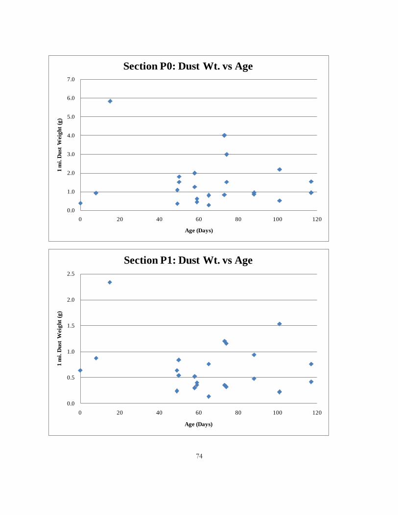
74

0.0

1.0

2.0

3.0

4.0

5.0

6.0

7.0

0 20 40 60 80 100 120

1 m

i. D

ust

Wei

ght (

g)

Age (Days)

Section P0: Dust Wt. vs Age

0.0

0.5

1.0

1.5

2.0

2.5

0 20 40 60 80 100 120

1 m

i. D

ust

Wei

ght (

g)

Age (Days)

Section P1: Dust Wt. vs Age

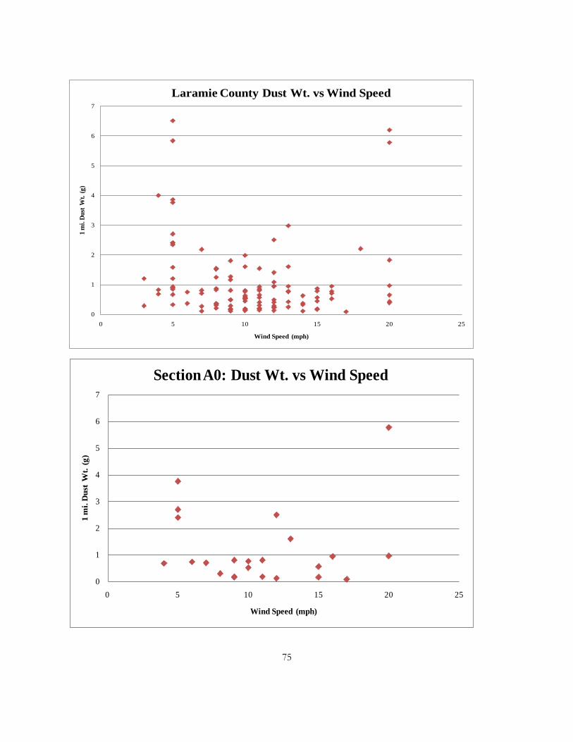
75

0

1

2

3

4

5

6

7

0 5 10 15 20 25

1 mi.

Dust

Wt.

(g)

Wind Speed (mph)

Laramie County Dust Wt. vs Wind Speed

0

1

2

3

4

5

6

7

0 5 10 15 20 25

1 m

i. D

ust

Wt.

(g)

Wind Speed (mph)

Section A0: Dust Wt. vs Wind Speed

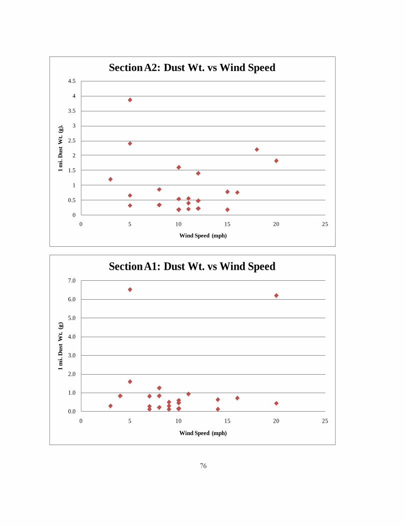
76

0

0.5

1

1.5

2

2.5

3

3.5

4

4.5

0 5 10 15 20 25

1 m

i. D

ust

Wt.

(g).

Wind Speed (mph)

Section A2: Dust Wt. vs Wind Speed

0.0

1.0

2.0

3.0

4.0

5.0

6.0

7.0

0 5 10 15 20 25

1 m

i. D

ust

Wt.

(g)

Wind Speed (mph)

Section A1: Dust Wt. vs Wind Speed

77

0.0

1.0

2.0

3.0

4.0

5.0

6.0

7.0

0 5 10 15 20 25

1 m

i. D

ust

Wt.

(g)

Wind Speed (mph)

Section P0: Dust Wt. vs Wind Speed

0

0.5

1

1.5

2

2.5

0 5 10 15 20 25

1 m

i. D

ust

Wt.

(g)

Wind Speed (mph)

Section P1: Dust Wt. vs Wind Speed

78

0

1

2

3

4

5

6

7

0.000 1.000 2.000 3.000 4.000 5.000 6.000 7.000

1 m

i. D

ust

Wt.

(g)

MC (%)

Laramie County Dust Wt. vs Moisture Content

0

1

2

3

4

5

6

7

0.000 1.000 2.000 3.000 4.000 5.000 6.000

1 m

i. D

ust

Wt.

(g)

MC (%)

Section A0: Dust Wt. vs MC

79

0

0.5

1

1.5

2

2.5

3

3.5

4

4.5

0.000 1.000 2.000 3.000 4.000 5.000 6.000 7.000

1 m

i. D

ust

Wt.

(g)

MC (%)

Section A2: Dust Wt. vs MC

0.00

1.00

2.00

3.00

4.00

5.00

6.00

7.00

0.000 0.500 1.000 1.500 2.000 2.500 3.000 3.500 4.000

1 m

i. D

ust

Wt.

(g)

MC (%)

Section A1: Dust Wt. vs MC

80

0

1

2

3

4

5

6

7

0.000 1.000 2.000 3.000 4.000 5.000 6.000

1 mi.

Dust

Wt.

(g)

MC (%)

Section P0: Dust Wt. vs MC

0

0.5

1

1.5

2

2.5

0 1 2 3 4 5 6

1 m

i. D

ust

Wt.

(g)

MC (%)

Section P1: Dust Wt. vs MC

81

1 Section 1 & 2 of RAP (no dust abatement) 6/9/2008 2:15 PM 10 NNW 1.50 2.1172 Section 1 & 2 of RAP (no dust abatement) 6/11/2008 9:05 AM 10 NNW 0.77 1.9043 Section 1 & 2 of RAP (no dust abatement) 6/17/2008 12:45 PM 10 NNW 1.84 0.3164 Schoonover Road - S0 (100% Gravel w/ CaCl) 7/14/2008 12:45 PM 15 NNW 1.08 1.6575 Schoonover Road - S2 (RAP Blend) 7/28/2008 4:00 PM 5 N 0.54 0.3486 Schoonover Road - S1 (RAP Blend w/ CaCl) 7/28/2008 4:10 PM 5 N 0.26 1.6927 Schoonover Road - S0 (100% Gravel w/ CaCl) 7/28/2008 4:20 PM 5 N 0.46 1.2828 Schoonover Road - S2 (RAP Blend) 7/28/2008 4:35 PM 5 N 0.54 0.3489 Schoonover Road - S1 (RAP Blend w/ CaCl) 7/28/2008 4:30 PM 5 N 0.48 1.692

10 Schoonover Road - S0 (100% Gravel w/ CaCl) 7/28/2008 4:25 PM 5 N 1.04 1.28211 Schoonover Road - S2 (RAP Blend) 7/29/2008 9:45 AM 0 0.86 0.50412 Schoonover Road - S1 (RAP Blend w/ CaCl) 7/29/2008 9:50 AM 0 0.48 1.56913 Schoonover Road - S0 (100% Gravel w/ CaCl) 7/29/2008 9:55 AM 0 1.52 1.74114 Schoonover Road - S2 (RAP Blend) 7/29/2008 9:40 AM 0 0.50 0.50415 Schoonover Road - S1 (RAP Blend w/ CaCl) 7/29/2008 9:30 AM 0 0.50 1.56916 Schoonover Road - S0 (100% Gravel w/ CaCl) 7/29/2008 9:20 AM 0 1.36 1.74117 Schoonover Road - S2 (RAP Blend) 8/6/2008 3:20 PM 3 N 0.64 0.33118 Schoonover Road - S1 (RAP Blend w/ CaCl) 8/6/2008 3:15 PM 4 NE 0.28 1.29719 Schoonover Road - S0 (100% Gravel w/ CaCl) 8/6/2008 3:10 PM 3 NE 0.98 0.69820 Schoonover Road - S2 (RAP Blend) 8/6/2008 2:40 PM 6 NE 0.36 0.33121 Schoonover Road - S1 (RAP Blend w/ CaCl) 8/6/2008 2:55 PM 2 N 0.22 1.29722 Schoonover Road - S0 (100% Gravel w/ CaCl) 8/6/2008 3:05 PM 0 0.50 0.69823 Schoonover Road - S2 (RAP Blend) 8/7/2008 10:35 AM 14 SSE 0.66 0.50924 Schoonover Road - S1 (RAP Blend w/ CaCl) 8/7/2008 9:55 AM 15 SSE 0.32 1.11825 Schoonover Road - S0 (100% Gravel w/ CaCl) 8/7/2008 10:10 AM 12 SSE 1.68 1.52326 Schoonover Road - S2 (RAP Blend) 8/7/2008 10:30 AM 16 SSE 0.14 0.50927 Schoonover Road - S1 (RAP Blend w/ CaCl) 8/7/2008 10:25 AM 18 SSE 0.20 1.11828 Schoonover Road - S0 (100% Gravel w/ CaCl) 8/7/2008 10:20 AM 17 SSE 0.90 1.52329 Schoonover Road - S2 (RAP Blend) 8/13/2008 3:35 PM 7 ESE 0.24 0.25130 Schoonover Road - S2 (RAP Blend) 8/13/2008 3:30 PM 3 ESE 0.66 0.25131 Schoonover Road - S1 (RAP Blend w/ CaCl) 8/13/2008 3:15 PM 5 SE 0.20 0.74332 Schoonover Road - S2 (RAP Blend) 8/14/2008 10:10 AM 10 WNW 0.18 0.27033 Schoonover Road - S2 (RAP Blend) 8/21/2008 12:30 PM 12 S 0.66 0.29134 Schoonover Road - S1 (RAP Blend w/ CaCl) 8/21/2008 12:45 PM 18 S 0.16 1.28035 Schoonover Road - S0 (100% Gravel w/ CaCl) 8/21/2008 12:55 PM 10 S 0.14 1.30136 Schoonover Road - S2 (RAP Blend) 8/21/2008 1:10 PM 15 S 0.16 0.29137 Schoonover Road - S1 (RAP Blend w/ CaCl) 8/21/2008 1:05 PM 13 S 0.12 1.28038 Schoonover Road - S0 (100% Gravel w/ CaCl) 8/21/2008 1:00 PM 11 S 0.12 1.30139 Schoonover Road - S2 (RAP Blend) 8/22/2008 7:45 AM 8 NNW 0.36 0.42240 Schoonover Road - S1 (RAP Blend w/ CaCl) 8/22/2008 8:00 AM 6 NW 0.14 1.31141 Schoonover Road - S0 (100% Gravel w/ CaCl) 8/22/2008 8:05 AM 9 WNW 0.20 1.78942 Schoonover Road - S2 (RAP Blend) 8/22/2008 8:20 AM 9 NW 0.90 0.42243 Schoonover Road - S1 (RAP Blend w/ CaCl) 8/22/2008 8:15 AM 7 NW 0.18 1.31144 Schoonover Road - S0 (100% Gravel w/ CaCl) 8/22/2008 8:10 AM 10 NNW 0.28 1.78945 Schoonover Road - S2 (RAP Blend) 9/1/2008 10:25 AM 5 NW 0.48 0.42946 Schoonover Road - S1 (RAP Blend w/ CaCl) 9/1/2008 10:20 AM 2 NW 0.30 2.10247 Schoonover Road - S0 (100% Gravel w/ CaCl) 9/1/2008 10:10 AM 3 NW 0.20 2.58448 Schoonover Road - S2 (RAP Blend) 9/1/2008 10:30 AM 5 NW 0.46 0.42949 Schoonover Road - S1 (RAP Blend w/ CaCl) 9/1/2008 10:35 AM 5 NW 0.12 2.10250 Schoonover Road - S0 (100% Gravel w/ CaCl) 9/1/2008 10:40 AM 4 NW 0.18 2.584

Johnson County Dust, Moisture Content, and Wind Data

# Test Section Date of Sample

Time of Sample Wind (mph) 1 mi. Dust

Wt. (g)Moisture

Content (%)

82

51 Schoonover Road - S2 (RAP Blend) 10/3/2008 6:50 PM 12 SSE 0.96 0.32652 Schoonover Road - S1 (RAP Blend w/ CaCl) 10/3/2008 7:05 PM 4 S 0.30 0.93953 Schoonover Road - S0 (100% Gravel w/ CaCl) 10/3/2008 7:10 PM 4 S 0.54 1.98054 Schoonover Road - S2 (RAP Blend) 10/3/2008 7:25 PM 7 S 0.26 0.32655 Schoonover Road - S1 (RAP Blend w/ CaCl) 10/3/2008 7:20 PM 6 S 0.20 0.93956 Schoonover Road - S0 (100% Gravel w/ CaCl) 10/3/2008 7:15 PM 5 S 0.28 1.98057 Schoonover Road - S2 (RAP Blend) 10/4/2008 8:00 AM 4 S 0.94 0.84458 Schoonover Road - S1 (RAP Blend w/ CaCl) 10/4/2008 8:20 AM 7 SSE 0.16 0.37659 Schoonover Road - S0 (100% Gravel w/ CaCl) 10/4/2008 8:25 AM 9 S 0.32 1.71360 Schoonover Road - S2 (RAP Blend) 10/4/2008 9:20 AM 16 S 0.10 0.84461 Schoonover Road - S1 (RAP Blend w/ CaCl) 10/4/2008 9:10 AM 14 S 0.08 0.37662 Schoonover Road - S0 (100% Gravel w/ CaCl) 10/4/2008 8:50 AM 12 S 0.14 1.713

Johnson County Dust, Moisture Content, and Wind Data

# Test Section Date of Sample

Time of Sample Wind (mph) 1 mi. Dust

Wt. (g)Moisture

Content (%)

0.0

0.2

0.4

0.6

0.8

1.0

1.2

1.4

1.6

1.8

2.0

0 20 40 60 80 100 120

1 m

i. D

ust

Wt.

(g)

Age (Days)

Johnson County Dust Wt. vs Age

83

0.0

0.2

0.4

0.6

0.8

1.0

1.2

1.4

1.6

1.8

2.0

0 20 40 60 80 100 120

1 m

i. D

ust

Wt.

(g)

Age (Days)

Section S2: Dust Wt. vs Age

0.0

0.1

0.2

0.3

0.4

0.5

0.6

0 20 40 60 80

1 m

i. D

ust

Wt.

(g)

Age (Days)

Section S1: Dust Wt. vs Age

84

0.0

0.2

0.4

0.6

0.8

1.0

1.2

1.4

1.6

1.8

0 20 40 60 80 100

1 m

i. D

ust

Wt.

(g)

Age (Days)

Section S0: Dust Wt. vs Age

0.0

0.2

0.4

0.6

0.8

1.0

1.2

1.4

1.6

1.8

2.0

0 2 4 6 8 10 12 14 16 18 20

1 m

i. D

ust

Wt.

(g)

Wind Speed (mph)

Johnson County Dust vs Wind Speed

85

0.0

0.2

0.4

0.6

0.8

1.0

1.2

1.4

1.6

1.8

2.0

0 2 4 6 8 10 12 14 16 18

1 mi.

Dust

Wt.

(g)

Wind Speed (mph)

Section S2: Dust vs Wind Speed

0.0

0.1

0.2

0.3

0.4

0.5

0.6

0 2 4 6 8 10 12 14 16 18 20

1 m

i. D

ust

Wt.

(g)

Wind Speed (mph)

Section S1: Dust vs Wind Speed

86

0.0

0.2

0.4

0.6

0.8

1.0

1.2

1.4

1.6

1.8

0 2 4 6 8 10 12 14 16

1 m

i. D

ust

Wt.

(g)

Wind Speed (mph)

Section S0: Dust vs Wind Speed

0.0

0.2

0.4

0.6

0.8

1.0

1.2

1.4

1.6

1.8

2.0

0.00 0.50 1.00 1.50 2.00 2.50 3.00

1 m

i. D

ust

Wt,

(g)

Moisture Content (%)

Johnson County Dust vs Moisture Content

87

0.0

0.2

0.4

0.6

0.8

1.0

1.2

1.4

1.6

1.8

2.0

0.00 0.50 1.00 1.50 2.00 2.50

1 m

i. D

ust

Wt.

(g)

Moisture Content (%)

Section S2: Dust vs Moisture Content

0.0

0.1

0.2

0.3

0.4

0.5

0.6

0.00 0.50 1.00 1.50 2.00 2.50

1 m

i. D

ust

Wt.

(g)

Moisture Content (%)

Section S1: Dust vs Moisture Content

88

0.0

0.2

0.4

0.6

0.8

1.0

1.2

1.4

1.6

1.8

0.00 0.50 1.00 1.50 2.00 2.50 3.00

1 m

i. D

ust

Wt.

(g)

Moisture Content (%)

Section S0: Dust vs Moisture Content

89

APPENDIX B UNSURFACED ROAD CONDITION INDEX INSPECTION SHEETS

90

Date URCI Date URCI6/24/2008 86 6/24/2008 957/11/2008 84 7/11/2008 957/28/2008 89 7/28/2008 908/6/2008 82 8/6/2008 90

8/13/2008 84 8/13/2008 908/22/2008 77 8/22/2008 909/5/2008 77 9/5/2008 90

9/18/2008 76 9/18/2008 9110/4/2008 83 10/4/2008 85

Date URCI Date URCI6/24/2008 100 6/24/2008 1007/11/2008 97 7/11/2008 1007/28/2008 92 7/28/2008 1008/6/2008 90 8/6/2008 100

8/13/2008 90 8/13/2008 1008/22/2008 90 8/22/2008 1009/5/2008 90 9/5/2008 100

9/18/2008 90 9/18/2008 10010/4/2008 90 10/4/2008 100

Date URCI6/24/2008 1007/11/2008 1007/28/2008 1008/6/2008 100

8/13/2008 1008/22/2008 939/5/2008 93

9/18/2008 9410/4/2008 97

Pry Road - P1 (1 1/2" RAP)

Pry Road - P0 (100% Gravel)

Laramie County URCI

Atlas Road - A2 (2 1/2" RAP)

Atlas Road - A1 (1 1/2" RAP)

Atlas Road - A0 (100% Gravel)

91

Date URCI7/14/2008 1007/29/2008 958/6/2008 95

8/13/2008 958/21/2008 929/1/2008 90

10/4/2008 88

Date URCI7/14/2008 1007/29/2008 1008/6/2008 90

8/13/2008 878/21/2008 879/1/2008 84

10/4/2008 88

Date URCI7/14/2008 1007/29/2008 978/6/2008 90

8/21/2008 859/1/2008 83

10/4/2008 65

Schoonover Road - S0 (100% Gravel w/ CaCl)

Johnson County URCI

Schoonover Road - S2 (RAP Blend)

Schoonover Road - S1 (RAP Blend w/ CaCl)

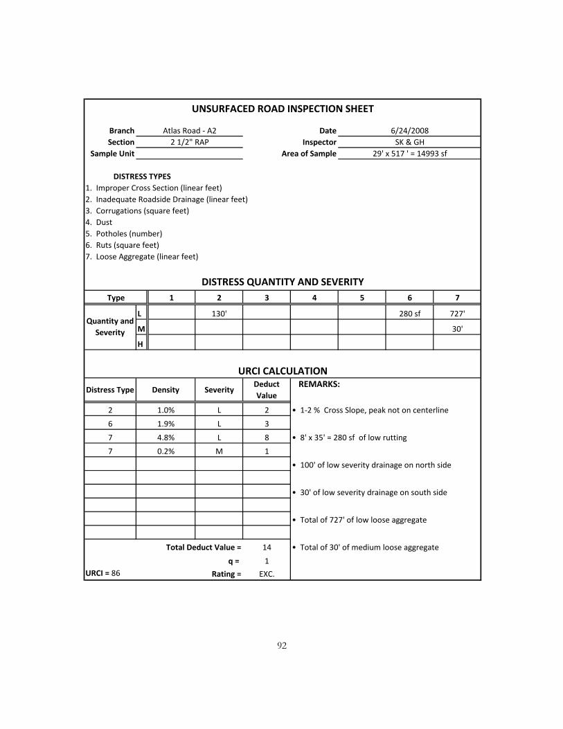
92

Branch DateSection Inspector

Sample Unit Area of Sample

DISTRESS TYPES1. Improper Cross Section (linear feet)2. Inadequate Roadside Drainage (linear feet)3. Corrugations (square feet)4. Dust5. Potholes (number)6. Ruts (square feet)7. Loose Aggregate (linear feet)

1 2 3 4 5 6 7

L 130' 280 sf 727'

M 30'

H

2 L 2 • 1-2 % Cross Slope, peak not on centerline

6 L 3

7 L 8 • 8' x 35' = 280 sf of low rutting

7 M 1

• 100' of low severity drainage on north side

• 30' of low severity drainage on south side

• Total of 727' of low loose aggregate

Total Deduct Value = 14 • Total of 30' of medium loose aggregate

q = 1URCI = 86 Rating = EXC.

0.2%

1.9%

4.8%

1.0%

Quantity and Severity

URCI CALCULATION

Distress Type Density SeverityDeduct Value

REMARKS:

DISTRESS QUANTITY AND SEVERITYType

29' x 517 ' = 14993 sf2 1/2" RAP SK & GH

UNSURFACED ROAD INSPECTION SHEET

Atlas Road - A2 6/24/2008

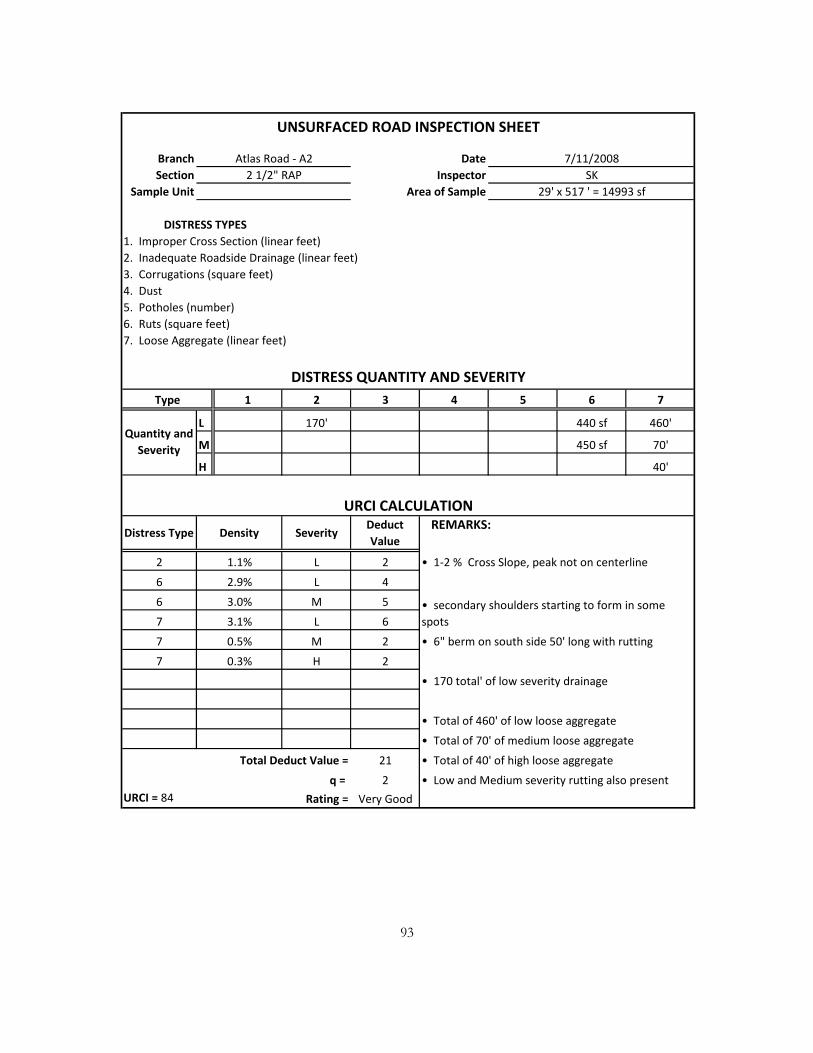
93

Branch DateSection Inspector

Sample Unit Area of Sample

DISTRESS TYPES1. Improper Cross Section (linear feet)2. Inadequate Roadside Drainage (linear feet)3. Corrugations (square feet)4. Dust5. Potholes (number)6. Ruts (square feet)7. Loose Aggregate (linear feet)

1 2 3 4 5 6 7

L 170' 440 sf 460'

M 450 sf 70'

H 40'

2 L 2 • 1-2 % Cross Slope, peak not on centerline

6 L 4

6 M 5

7 L 6

7 M 2 • 6" berm on south side 50' long with rutting

7 H 2

• 170 total' of low severity drainage

• Total of 460' of low loose aggregate

• Total of 70' of medium loose aggregate

Total Deduct Value = 21 • Total of 40' of high loose aggregate

q = 2 • Low and Medium severity rutting also presentURCI = 84 Rating = Very Good

• secondary shoulders starting to form in some spots

0.3%

3.1%

0.5%

2.9%

3.0%

1.1%

Distress Type Density SeverityDeduct Value

REMARKS:

Quantity and Severity

URCI CALCULATION

DISTRESS QUANTITY AND SEVERITYType

29' x 517 ' = 14993 sf2 1/2" RAP SK

UNSURFACED ROAD INSPECTION SHEET

Atlas Road - A2 7/11/2008

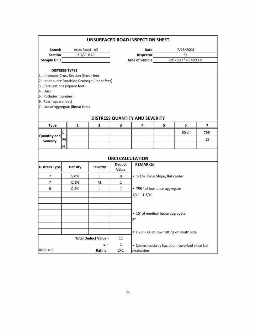
94

Branch DateSection Inspector

Sample Unit Area of Sample

DISTRESS TYPES1. Improper Cross Section (linear feet)2. Inadequate Roadside Drainage (linear feet)3. Corrugations (square feet)4. Dust5. Potholes (number)6. Ruts (square feet)7. Loose Aggregate (linear feet)

1 2 3 4 5 6 7

L 60 sf 755'

M 15

H

7 L 9 • 1-2 % Cross Slope, flat center

7 M 1

6 L 1 • 755 ' of low loose aggregate

1/2" - 1 3/4"

• 15' of medium loose aggregate

2"

3' x 20' = 60 sf low rutting on south side

Total Deduct Value = 11

q = 1URCI = 89 Rating = EXC.

• Seems roadway has been reworked since last evaluation

0.1%

0.4%

5.0%

Density SeverityDeduct Value

REMARKS:

Quantity and Severity

Distress Type

URCI CALCULATION

DISTRESS QUANTITY AND SEVERITYType

29' x 517 ' = 14993 sf2 1/2" RAP SK

UNSURFACED ROAD INSPECTION SHEET

Atlas Road - A2 7/28/2008

95

Branch DateSection Inspector

Sample Unit Area of Sample

DISTRESS TYPES1. Improper Cross Section (linear feet)2. Inadequate Roadside Drainage (linear feet)3. Corrugations (square feet)4. Dust5. Potholes (number)6. Ruts (square feet)7. Loose Aggregate (linear feet)

1 2 3 4 5 6 7

L 220 sf 1059'

M 200 sf 50'

H

7 L 12 • 1-2 % Cross Slope, peak not on centerline

7 M 3 flat center

6 L 2 • Medium rutting on south side

6 M 2 4' x 50' = 200 sf

• Low rutting on south side

4' x 30' = 120 sf

• Low rutting on north side

2' x 50' = 100 sf

• Total of 1059' of low loose aggregate

Total Deduct Value = 19

q = 1 • 50' of medium loose aggregate on south sideURCI = 82 Rating = Very Good

1.3%

0.3%

1.5%

7.1%

SeverityDeduct Value

REMARKS:Distress Type Density

Quantity and Severity

URCI CALCULATION

DISTRESS QUANTITY AND SEVERITYType

29' x 517 ' = 14993 sf2 1/2" RAP SK

UNSURFACED ROAD INSPECTION SHEET

Atlas Road - A2 8/6/2008

96

Branch DateSection Inspector

Sample Unit Area of Sample

DISTRESS TYPES1. Improper Cross Section (linear feet)2. Inadequate Roadside Drainage (linear feet)3. Corrugations (square feet)4. Dust5. Potholes (number)6. Ruts (square feet)7. Loose Aggregate (linear feet)

1 2 3 4 5 6 7

L 220 sf 1064'

M 200 sf 100'

H

6 L 2 • 1% Cross Slope not on centerline. Flat center

6 M 2

7 L 12 • Total of 1064' low loose aggregate

7 M 5

• 100' of medium loose aggregate on south side

• 200 sf of medium rutting on south side

• 120 sf of low rutting on south side

Total Deduct Value = 21 • 100 sf of low rutting on north side

q = 2URCI = 84 Rating = Very Good

0.7%

1.3%

7.1%

1.5%

Distress Type Density

Quantity and Severity

URCI CALCULATIONDeduct Value

REMARKS:Severity

DISTRESS QUANTITY AND SEVERITYType

SK29' x 517 ' = 14993 sf

2 1/2" RAP

UNSURFACED ROAD INSPECTION SHEET

Atlas Road - A2 8/13/2008

97

Branch DateSection Inspector

Sample Unit Area of Sample

DISTRESS TYPES1. Improper Cross Section (linear feet)2. Inadequate Roadside Drainage (linear feet)3. Corrugations (square feet)4. Dust5. Potholes (number)6. Ruts (square feet)7. Loose Aggregate (linear feet)

1 2 3 4 5 6 7

L 10 250 sf 1064'

M 400 sf 130'

H

6 L 2 • 1% Cross Slope not on centerline. Flat center

6 M 3

7 L 12 • Total of 1064' low loose aggregate

7 M 4 • 80' of medium loose aggregate on south side

5 L 10 (east)

• 50' of medium loose aggregate on south side

(west)

Total Deduct Value = 23 • >1' diameter potholes on west end

q = 1 10 at 1" deepURCI = 77 Rating = Very Good

• Low and medium rutting on south side (east and west)

1.7%

2.7%

7.1%

0.9%

0.07%

DISTRESS QUANTITY AND SEVERITYType

Quantity and Severity

URCI CALCULATION

Distress Type Density SeverityDeduct Value

REMARKS:

UNSURFACED ROAD INSPECTION SHEET

Atlas Road - A2 8/22/20082 1/2" RAP SK

29' x 517 ' = 14993 sf

98

Branch DateSection Inspector

Sample Unit Area of Sample

DISTRESS TYPES1. Improper Cross Section (linear feet)2. Inadequate Roadside Drainage (linear feet)3. Corrugations (square feet)4. Dust5. Potholes (number)6. Ruts (square feet)7. Loose Aggregate (linear feet)

1 2 3 4 5 6 7

L 10 250 sf 1034'

M 400 sf 300'

H

5 L 2 • 1% Cross Slope not on centerline. Flat center

6 L 2 • 1034' low loose aggregate from both sides

6 M 3 • 300' med loose aggregate on south side

7 L 12

7 M 10

• 30' x 3' = 90sf of low rutting (middle)

(west)

• 40' x 4' = 160 sf low rutting south (east)

• 20' x 4' = 80 sf medium rutting north (west)

Total Deduct Value = 29 • >1' diameter potholes on west end

q = 2 10 at 1" deepURCI = 77 Rating = Very Good

UNSURFACED ROAD INSPECTION SHEET

Atlas Road - A2 9/5/20082 1/2" RAP SK

29' x 517 ' = 14993 sf

DISTRESS QUANTITY AND SEVERITYType

Quantity and Severity

URCI CALCULATION

Distress Type Density SeverityDeduct Value

REMARKS:

0.07%

1.7%

2.7%

7.1%

2.0% • 80' x 4' = 320sf of medium rutting on south side

99

Branch DateSection Inspector

Sample Unit Area of Sample

DISTRESS TYPES1. Improper Cross Section (linear feet)2. Inadequate Roadside Drainage (linear feet)3. Corrugations (square feet)4. Dust5. Potholes (number)6. Ruts (square feet)7. Loose Aggregate (linear feet)

1 2 3 4 5 6 7

L 10 320 sf 1264'

M 300 sf 45'

H 30'

5 L 2 • 1% Cross Slope not on centerline. Flat center

6 L 2 • 1034' low loose aggregate from both sides

6 M 3 • 30' low loose aggregate middle (west)

7 L 12 • 200' low loose aggregate middle( east)

7 M 2 • 45' med loose aggregate south (east)

7 H 2 • 30' high loose aggregate south (east)

• 35' x 4' = 140 sf low rutting middle (west)

• 60' x 3' = 180 sf low rutting middle (east)

• 50' x 6' = 300 sf med rutting middle (east)

Total Deduct Value = 22 • >1' diameter potholes on west end

q = 1 10 at 1" deepURCI = 79 Rating = Very Good

UNSURFACED ROAD INSPECTION SHEET

Atlas Road - A2 9/18/20082 1/2" RAP SK

29' x 517 ' = 14993 sf

DISTRESS QUANTITY AND SEVERITYType

2.7%

7.1%

0.3%

0.2%

Quantity and Severity

URCI CALCULATION

Distress Type Density SeverityDeduct Value

REMARKS:

0.07%

1.7%

100

Branch DateSection Inspector

Sample Unit Area of Sample

DISTRESS TYPES1. Improper Cross Section (linear feet)2. Inadequate Roadside Drainage (linear feet)3. Corrugations (square feet)4. Dust5. Potholes (number)6. Ruts (square feet)7. Loose Aggregate (linear feet)

1 2 3 4 5 6 7

L 10 625 sf 1134'

M

H 30'

5 L 2 • 1% Cross Slope not on centerline. Flat center

6 L 7 • 1034' low loose aggregate from both sides

7 L 12 < 2"

7 H 2 • 100' low loose aggregate middle( east)

• 30' high loose aggregate south (east)

• 30' x2' = 60 sf low rutting middle

• 45' x 3' = 135 sf low rutting middle (east)

• 50' x 5' = 250 sf med rutting middle (east)

Total Deduct Value = 23 • >1' diameter potholes on west end

q = 2 10 at 1" deepURCI = 83 Rating = Very Good

UNSURFACED ROAD INSPECTION SHEET

Atlas Road - A2 10/4/20082 1/2" RAP SK

29' x 517 ' = 14993 sf

DISTRESS QUANTITY AND SEVERITYType

Quantity and Severity

URCI CALCULATION

Distress Type Density SeverityDeduct Value

REMARKS:

0.07%

4.2%

7.6%

0.2%

101

Branch DateSection Inspector

Sample Unit Area of Sample

DISTRESS TYPES1. Improper Cross Section (linear feet)2. Inadequate Roadside Drainage (linear feet)3. Corrugations (square feet)4. Dust5. Potholes (number)6. Ruts (square feet)7. Loose Aggregate (linear feet)

1 2 3 4 5 6 7

L

M

H

• 3 % Cross Slope

• No Distresses

Total Deduct Value = 0q = 0

URCI = 100 Rating = EXC.

Quantity and Severity

URCI CALCULATION

Distress Type Density SeverityDeduct Value

REMARKS:

DISTRESS QUANTITY AND SEVERITYType

30' x 100 ' = 3000 sf1 1/2" RAP SK & GH

UNSURFACED ROAD INSPECTION SHEET

Atlas Road - A1 6/24/2008

102

Branch DateSection Inspector

Sample Unit Area of Sample

DISTRESS TYPES1. Improper Cross Section (linear feet)2. Inadequate Roadside Drainage (linear feet)3. Corrugations (square feet)4. Dust5. Potholes (number)6. Ruts (square feet)7. Loose Aggregate (linear feet)

1 2 3 4 5 6 7

L 65'

M

H

7 L 4 • 3 % Cross Slope

• 40' of low loose aggregate on north side

• 25' of low loose aggregate on south side

1/2" - 3/4"

Total Deduct Value = 4q = 0

URCI = 97 Rating = EXC.

2.2%

Distress Type Density SeverityDeduct Value

REMARKS:

Quantity and Severity

URCI CALCULATION

DISTRESS QUANTITY AND SEVERITYType

3000 sf1 1/2" RAP SK

UNSURFACED ROAD INSPECTION SHEET

Atlas Road - A1 7/11/2008

103

Branch DateSection Inspector

Sample Unit Area of Sample

DISTRESS TYPES1. Improper Cross Section (linear feet)2. Inadequate Roadside Drainage (linear feet)3. Corrugations (square feet)4. Dust5. Potholes (number)6. Ruts (square feet)7. Loose Aggregate (linear feet)

1 2 3 4 5 6 7

L 150'

M

H

7 L 9 • 2 % Cross Slope

• 100' of low loose aggregate on north side

• 50' of low loose aggregate on south side

1/2" - 1"

Total Deduct Value = 9q = 1

URCI = 92 Rating = EXC.

5.0%

Density SeverityDeduct Value

REMARKS:

Quantity and Severity

Distress Type

URCI CALCULATION

DISTRESS QUANTITY AND SEVERITYType

3000 sf1 1/2" RAP SK

UNSURFACED ROAD INSPECTION SHEET

Atlas Road - A1 7/28/2008

104

Branch DateSection Inspector

Sample Unit Area of Sample

DISTRESS TYPES1. Improper Cross Section (linear feet)2. Inadequate Roadside Drainage (linear feet)3. Corrugations (square feet)4. Dust5. Potholes (number)6. Ruts (square feet)7. Loose Aggregate (linear feet)

1 2 3 4 5 6 7

L 200'

M

H

7 L 11 • 2 % Cross Slope

• 100' of low loose aggregate on north side

1/2" - 1"

• 100' of low loose aggregate on south side

1/2" - 1 1/4"

Total Deduct Value = 11q = 1

URCI = 90 Rating = EXC.

6.7%

SeverityDeduct Value

REMARKS:Distress Type Density

Quantity and Severity

URCI CALCULATION

DISTRESS QUANTITY AND SEVERITYType

3000 sf1 1/2" RAP SK

UNSURFACED ROAD INSPECTION SHEET

Atlas Road - A1 8/6/2008

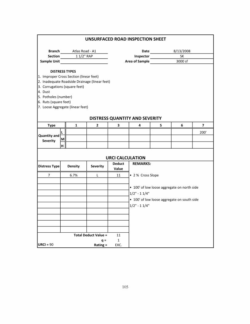
105

Branch DateSection Inspector

Sample Unit Area of Sample

DISTRESS TYPES1. Improper Cross Section (linear feet)2. Inadequate Roadside Drainage (linear feet)3. Corrugations (square feet)4. Dust5. Potholes (number)6. Ruts (square feet)7. Loose Aggregate (linear feet)

1 2 3 4 5 6 7

L 200'

M

H

7 L 11 • 2 % Cross Slope

• 100' of low loose aggregate on north side

1/2" - 1 1/4"

• 100' of low loose aggregate on south side

1/2" - 1 1/4"

Total Deduct Value = 11q = 1

URCI = 90 Rating = EXC.

6.7%

Distress Type Density

Quantity and Severity

URCI CALCULATIONDeduct Value

REMARKS:Severity

DISTRESS QUANTITY AND SEVERITYType

SK3000 sf

1 1/2" RAP

UNSURFACED ROAD INSPECTION SHEET

Atlas Road - A1 8/13/2008

106

Branch DateSection Inspector

Sample Unit Area of Sample

DISTRESS TYPES1. Improper Cross Section (linear feet)2. Inadequate Roadside Drainage (linear feet)3. Corrugations (square feet)4. Dust5. Potholes (number)6. Ruts (square feet)7. Loose Aggregate (linear feet)

1 2 3 4 5 6 7

L 200'

M

H

7 L 11 • 2% Cross Slope

• 100' of low loose aggregate on north side

1/2" - 1 1/4"

• 100' of low loose aggregate on south side

1/2" - 1 1/4"

• no rutting but rough surface

Total Deduct Value = 11q = 1

URCI = 90 Rating = EXC.

6.7%

DISTRESS QUANTITY AND SEVERITYType

Quantity and Severity

URCI CALCULATION

Distress Type Density SeverityDeduct Value

REMARKS:

Atlas Road - A1 8/22/20081 1/2" RAP SK

3000 sf

UNSURFACED ROAD INSPECTION SHEET

107

Branch DateSection Inspector

Sample Unit Area of Sample

DISTRESS TYPES1. Improper Cross Section (linear feet)2. Inadequate Roadside Drainage (linear feet)3. Corrugations (square feet)4. Dust5. Potholes (number)6. Ruts (square feet)7. Loose Aggregate (linear feet)

1 2 3 4 5 6 7

L 200'

M

H

7 L 11 • 2% Cross Slope

• 100' of low loose aggregate on north side

3/4" - 1 1/4"

• 100' of low loose aggregate on south side

1/2" - 1 1/4"

Total Deduct Value = 11q = 1

URCI = 90 Rating = EXC.

UNSURFACED ROAD INSPECTION SHEET

Atlas Road - A1 9/5/20081 1/2" RAP SK

3000 sf

DISTRESS QUANTITY AND SEVERITYType

Quantity and Severity

URCI CALCULATION

Distress Type Density SeverityDeduct Value

REMARKS:

6.7%

108

Branch DateSection Inspector

Sample Unit Area of Sample

DISTRESS TYPES1. Improper Cross Section (linear feet)2. Inadequate Roadside Drainage (linear feet)3. Corrugations (square feet)4. Dust5. Potholes (number)6. Ruts (square feet)7. Loose Aggregate (linear feet)

1 2 3 4 5 6 7

L 200'

M

H

7 L 11 • 2% Cross Slope

• 100' of low loose aggregate on both sides

3/4" - 1 1/2"

Total Deduct Value = 11q = 1

URCI = 90 Rating = EXC.

URCI CALCULATION

Distress Type Density SeverityDeduct Value

REMARKS:

6.7%

UNSURFACED ROAD INSPECTION SHEET

Atlas Road - A1 9/18/20081 1/2" RAP SK

3000 sf

DISTRESS QUANTITY AND SEVERITYType

Quantity and Severity

109

Branch DateSection Inspector

Sample Unit Area of Sample

DISTRESS TYPES1. Improper Cross Section (linear feet)2. Inadequate Roadside Drainage (linear feet)3. Corrugations (square feet)4. Dust5. Potholes (number)6. Ruts (square feet)7. Loose Aggregate (linear feet)

1 2 3 4 5 6 7

L 200'

M

H

7 L 11 • 2% Cross Slope

• 100' of low loose aggregate on both sides

3/4" - 1 1/2"

Total Deduct Value = 11q = 1

URCI = 90 Rating = EXC.

UNSURFACED ROAD INSPECTION SHEET

Atlas Road - A1 10/4/20081 1/2" RAP SK

3000 sf

DISTRESS QUANTITY AND SEVERITYType

Quantity and Severity

URCI CALCULATION

Distress Type Density SeverityDeduct Value

REMARKS:

6.7%

110

Branch DateSection Inspector

Sample Unit Area of Sample

DISTRESS TYPES1. Improper Cross Section (linear feet)2. Inadequate Roadside Drainage (linear feet)3. Corrugations (square feet)4. Dust5. Potholes (number)6. Ruts (square feet)7. Loose Aggregate (linear feet)

1 2 3 4 5 6 7

L

M

H

• 2 % Cross Slope

• No Distresses

Total Deduct Value = 0q = 0

URCI = 100 Rating = EXC.

Quantity and Severity

URCI CALCULATION

Distress Type Density SeverityDeduct Value

REMARKS:

DISTRESS QUANTITY AND SEVERITYType

27' x 100 ' = 2700 sf100 % Gravel SK & GH

UNSURFACED ROAD INSPECTION SHEET

Atlas Road - A0 6/24/2008

111

Branch DateSection Inspector

Sample Unit Area of Sample

DISTRESS TYPES1. Improper Cross Section (linear feet)2. Inadequate Roadside Drainage (linear feet)3. Corrugations (square feet)4. Dust5. Potholes (number)6. Ruts (square feet)7. Loose Aggregate (linear feet)

1 2 3 4 5 6 7

L

M

H

• 2 % Cross Slope

• No Distresses

Total Deduct Value = 0q = 0

URCI = 100 Rating = EXC.

Distress Type Density SeverityDeduct Value

REMARKS:

Quantity and Severity

URCI CALCULATION

DISTRESS QUANTITY AND SEVERITYType

27' x 100 ' = 2700 sf100 % Gravel SK

UNSURFACED ROAD INSPECTION SHEET

Atlas Road - A0 7/11/2008

112

Branch DateSection Inspector

Sample Unit Area of Sample

DISTRESS TYPES1. Improper Cross Section (linear feet)2. Inadequate Roadside Drainage (linear feet)3. Corrugations (square feet)4. Dust5. Potholes (number)6. Ruts (square feet)7. Loose Aggregate (linear feet)

1 2 3 4 5 6 7

L

M

H

• 2 % Cross Slope

• No Distresses

Total Deduct Value = 0q = 0

URCI = 100 Rating = EXC.

Density SeverityDeduct Value

REMARKS:

Quantity and Severity

Distress Type

URCI CALCULATION

DISTRESS QUANTITY AND SEVERITYType

27' x 100 ' = 2700 sf100 % Gravel SK

UNSURFACED ROAD INSPECTION SHEET

Atlas Road - A0 7/28/2008

113

Branch DateSection Inspector

Sample Unit Area of Sample

DISTRESS TYPES1. Improper Cross Section (linear feet)2. Inadequate Roadside Drainage (linear feet)3. Corrugations (square feet)4. Dust5. Potholes (number)6. Ruts (square feet)7. Loose Aggregate (linear feet)

1 2 3 4 5 6 7

L

M

H

• 2 % Cross Slope

• No Distresses

Total Deduct Value = 0q = 0

URCI = 100 Rating = EXC.

SeverityDeduct Value

REMARKS:Distress Type Density

Quantity and Severity

URCI CALCULATION

DISTRESS QUANTITY AND SEVERITYType

27' x 100 ' = 2700 sf100 % Gravel SK

UNSURFACED ROAD INSPECTION SHEET

Atlas Road - A0 8/6/2008

114

Branch DateSection Inspector

Sample Unit Area of Sample

DISTRESS TYPES1. Improper Cross Section (linear feet)2. Inadequate Roadside Drainage (linear feet)3. Corrugations (square feet)4. Dust5. Potholes (number)6. Ruts (square feet)7. Loose Aggregate (linear feet)

1 2 3 4 5 6 7

L

M

H

• 2 % Cross Slope

• No Distresses

Total Deduct Value = 0q = 0

URCI = 100 Rating = EXC.

Distress Type Density

Quantity and Severity

URCI CALCULATIONDeduct Value

REMARKS:Severity

DISTRESS QUANTITY AND SEVERITYType

SK27' x 100 ' = 2700 sf

100 % Gravel

UNSURFACED ROAD INSPECTION SHEET

Atlas Road - A0 8/13/2008

115

Branch DateSection Inspector

Sample Unit Area of Sample

DISTRESS TYPES1. Improper Cross Section (linear feet)2. Inadequate Roadside Drainage (linear feet)3. Corrugations (square feet)4. Dust5. Potholes (number)6. Ruts (square feet)7. Loose Aggregate (linear feet)

1 2 3 4 5 6 7

L 100'

M

H

7 L 8 • 2 % Cross Slope

• 100' of low loose aggregate on south side

1/2" - 1"

Total Deduct Value = 8q = 1

URCI = 93 Rating = EXC.

3.7%

Quantity and Severity

URCI CALCULATION

Distress Type Density SeverityDeduct Value

REMARKS:

100 % Gravel SK27' x 100 ' = 2700 sf

DISTRESS QUANTITY AND SEVERITYType

UNSURFACED ROAD INSPECTION SHEET

Atlas Road - A0 8/22/2008

116

Branch DateSection Inspector

Sample Unit Area of Sample

DISTRESS TYPES1. Improper Cross Section (linear feet)2. Inadequate Roadside Drainage (linear feet)3. Corrugations (square feet)4. Dust5. Potholes (number)6. Ruts (square feet)7. Loose Aggregate (linear feet)

1 2 3 4 5 6 7

L 100'

M

H

7 L 8 • 2 % Cross Slope

• 100' of low loose aggregate on south side

1/2" - 1"

Total Deduct Value = 8q = 1

URCI = 93 Rating = EXC.

UNSURFACED ROAD INSPECTION SHEET

Atlas Road - A0 9/5/2008100 % Gravel SK

27' x 100 ' = 2700 sf

DISTRESS QUANTITY AND SEVERITYType

Quantity and Severity

URCI CALCULATION

Distress Type Density SeverityDeduct Value

REMARKS:

3.7%

117

Branch DateSection Inspector

Sample Unit Area of Sample

DISTRESS TYPES1. Improper Cross Section (linear feet)2. Inadequate Roadside Drainage (linear feet)3. Corrugations (square feet)4. Dust5. Potholes (number)6. Ruts (square feet)7. Loose Aggregate (linear feet)

1 2 3 4 5 6 7

L 80'

M

H

7 L 6 • 2 % Cross Slope

• 80' of low loose aggregate on south side

1/2" - 1"

Total Deduct Value = 6q = 1

URCI = 94 Rating = EXC.

URCI CALCULATION

Distress Type Density SeverityDeduct Value

REMARKS:

3.0%

Atlas Road - A0 9/18/2008100 % Gravel SK

27' x 100 ' = 2700 sf

DISTRESS QUANTITY AND SEVERITYType

Quantity and Severity

UNSURFACED ROAD INSPECTION SHEET

118

Branch DateSection Inspector

Sample Unit Area of Sample

DISTRESS TYPES1. Improper Cross Section (linear feet)2. Inadequate Roadside Drainage (linear feet)3. Corrugations (square feet)4. Dust5. Potholes (number)6. Ruts (square feet)7. Loose Aggregate (linear feet)

1 2 3 4 5 6 7

L 55'

M

H

7 L 4 • 2 % Cross Slope

• 55' of low loose aggregate on south side

1/2" - 1"

Total Deduct Value = 4q = 1

URCI = 97 Rating = EXC.

UNSURFACED ROAD INSPECTION SHEET

Atlas Road - A0 10/4/2008100 % Gravel SK

27' x 100 ' = 2700 sf

DISTRESS QUANTITY AND SEVERITYType

Quantity and Severity

URCI CALCULATION

Distress Type Density SeverityDeduct Value

REMARKS:

2.0%

119

Branch DateSection Inspector

Sample Unit Area of Sample

DISTRESS TYPES1. Improper Cross Section (linear feet)2. Inadequate Roadside Drainage (linear feet)3. Corrugations (square feet)4. Dust5. Potholes (number)6. Ruts (square feet)7. Loose Aggregate (linear feet)

1 2 3 4 5 6 7

L 100'

M

H

7 L 6 • 3 % Cross Slope

• 100' low loose aggregate on west side

1/2" - 3/4"

Total Deduct Value = 6q = 1

URCI = 95 Rating = EXC.

DISTRESS QUANTITY AND SEVERITYType

Quantity and Severity

URCI CALCULATION

Distress Type Density SeverityDeduct Value

REMARKS:

UNSURFACED ROAD INSPECTION SHEET

Pry Road - P1 6/24/20081 1/2" RAP SK & GH

29' x 100 ' = 2900 sf

3.5%

120

Branch DateSection Inspector

Sample Unit Area of Sample

DISTRESS TYPES1. Improper Cross Section (linear feet)2. Inadequate Roadside Drainage (linear feet)3. Corrugations (square feet)4. Dust5. Potholes (number)6. Ruts (square feet)7. Loose Aggregate (linear feet)

1 2 3 4 5 6 7

L 100'

M

H

7 L 6 • 3 % Cross Slope

• 100' low loose aggregate on west side

1/2" - 3/4"

Total Deduct Value = 6q = 1

URCI = 95 Rating = EXC.

3.5%

DISTRESS QUANTITY AND SEVERITYType

Quantity and Severity

URCI CALCULATION

Distress Type Density SeverityDeduct Value

REMARKS:

UNSURFACED ROAD INSPECTION SHEET

Pry Road - P1 7/11/20081 1/2" RAP SK

2900 sf

121

Branch DateSection Inspector

Sample Unit Area of Sample

DISTRESS TYPES1. Improper Cross Section (linear feet)2. Inadequate Roadside Drainage (linear feet)3. Corrugations (square feet)4. Dust5. Potholes (number)6. Ruts (square feet)7. Loose Aggregate (linear feet)

1 2 3 4 5 6 7

L 200'

M

H

7 L 11 • 3 % Cross Slope

• 100' low loose aggregate on west side

3/4" - 1 1/4"

• 100' low loose aggregate on east side

1/2" - 1"

Total Deduct Value = 11q = 1

URCI = 90 Rating = EXC.

6.9%

2900 sf

DISTRESS QUANTITY AND SEVERITYType

Quantity and Severity

URCI CALCULATION

Distress Type Density SeverityDeduct Value

REMARKS:

UNSURFACED ROAD INSPECTION SHEET

Pry Road - P1 7/28/20081 1/2" RAP SK

122

Branch DateSection Inspector

Sample Unit Area of Sample

DISTRESS TYPES1. Improper Cross Section (linear feet)2. Inadequate Roadside Drainage (linear feet)3. Corrugations (square feet)4. Dust5. Potholes (number)6. Ruts (square feet)7. Loose Aggregate (linear feet)

1 2 3 4 5 6 7

L 200'

M

H

7 L 11 • 3 % Cross Slope

• 100' low loose aggregate on west side

3/4" - 1"

• 100' low loose aggregate on east side

1/2" - 1"

Total Deduct Value = 11q = 1

URCI = 90 Rating = EXC.

UNSURFACED ROAD INSPECTION SHEET

Pry Road - P1 8/6/20081 1/2" RAP SK

6.9%

2900 sf

DISTRESS QUANTITY AND SEVERITYType

Quantity and Severity

URCI CALCULATION

Distress Type Density SeverityDeduct Value

REMARKS:

123

Branch DateSection Inspector

Sample Unit Area of Sample

DISTRESS TYPES1. Improper Cross Section (linear feet)2. Inadequate Roadside Drainage (linear feet)3. Corrugations (square feet)4. Dust5. Potholes (number)6. Ruts (square feet)7. Loose Aggregate (linear feet)

1 2 3 4 5 6 7

L 200'

M

H

7 L 11 • 3 % Cross Slope

• 100' low loose aggregate on west side

1/2" - 1"

• 100' low loose aggregate on east side

1/2" - 1"

Total Deduct Value = 11q = 1

URCI = 90 Rating = EXC.

6.9%

2900 sf

DISTRESS QUANTITY AND SEVERITYType

Quantity and Severity

URCI CALCULATION

Distress Type Density SeverityDeduct Value

REMARKS:

UNSURFACED ROAD INSPECTION SHEET

Pry Road - P1 8/13/20081 1/2" RAP SK

124

Branch DateSection Inspector

Sample Unit Area of Sample

DISTRESS TYPES1. Improper Cross Section (linear feet)2. Inadequate Roadside Drainage (linear feet)3. Corrugations (square feet)4. Dust5. Potholes (number)6. Ruts (square feet)7. Loose Aggregate (linear feet)

1 2 3 4 5 6 7

L 200'

M

H

7 L 11 • 3 % Cross Slope

• 100' low loose aggregate on west side

3/4" - 1"

• 100' low loose aggregate on east side

3/4" - 1"

Total Deduct Value = 11q = 1

URCI = 90 Rating = EXC.

Distress Type Density SeverityDeduct Value

REMARKS:

6.9%

UNSURFACED ROAD INSPECTION SHEET

Pry Road - P1 8/22/20081 1/2" RAP SK

2900 sf

DISTRESS QUANTITY AND SEVERITYType

Quantity and Severity

URCI CALCULATION

125

Branch DateSection Inspector

Sample Unit Area of Sample

DISTRESS TYPES1. Improper Cross Section (linear feet)2. Inadequate Roadside Drainage (linear feet)3. Corrugations (square feet)4. Dust5. Potholes (number)6. Ruts (square feet)7. Loose Aggregate (linear feet)

1 2 3 4 5 6 7

L 200'

M

H

7 L 11 • 3 % Cross Slope

• 100' low loose aggregate on west side

• 100' low loose aggregate on east side

1/2" - 1 1/4"

Total Deduct Value = 11q = 1

URCI = 90 Rating = EXC.

UNSURFACED ROAD INSPECTION SHEET

Pry Road - P1 9/5/20081 1/2" RAP SK

2900 sf

DISTRESS QUANTITY AND SEVERITYType

Quantity and Severity

URCI CALCULATION

Distress Type Density SeverityDeduct Value

REMARKS:

6.9%

126

Branch DateSection Inspector

Sample Unit Area of Sample

DISTRESS TYPES1. Improper Cross Section (linear feet)2. Inadequate Roadside Drainage (linear feet)3. Corrugations (square feet)4. Dust5. Potholes (number)6. Ruts (square feet)7. Loose Aggregate (linear feet)

1 2 3 4 5 6 7

L 140'

M

H

7 L 9 • 3 % Cross Slope

• 100' low loose aggregate on west side

1/2" - 1 1/4"

• 40' low loose aggregate on east side

1/2" - 3/4 "

Total Deduct Value = 9q = 1

URCI = 91 Rating = EXC.

4.8%

1 1/2" RAP SK2900 sf

DISTRESS QUANTITY AND SEVERITYType

Quantity and Severity

URCI CALCULATION

Distress Type Density SeverityDeduct Value

REMARKS:

UNSURFACED ROAD INSPECTION SHEET

Pry Road - P1 9/18/2008

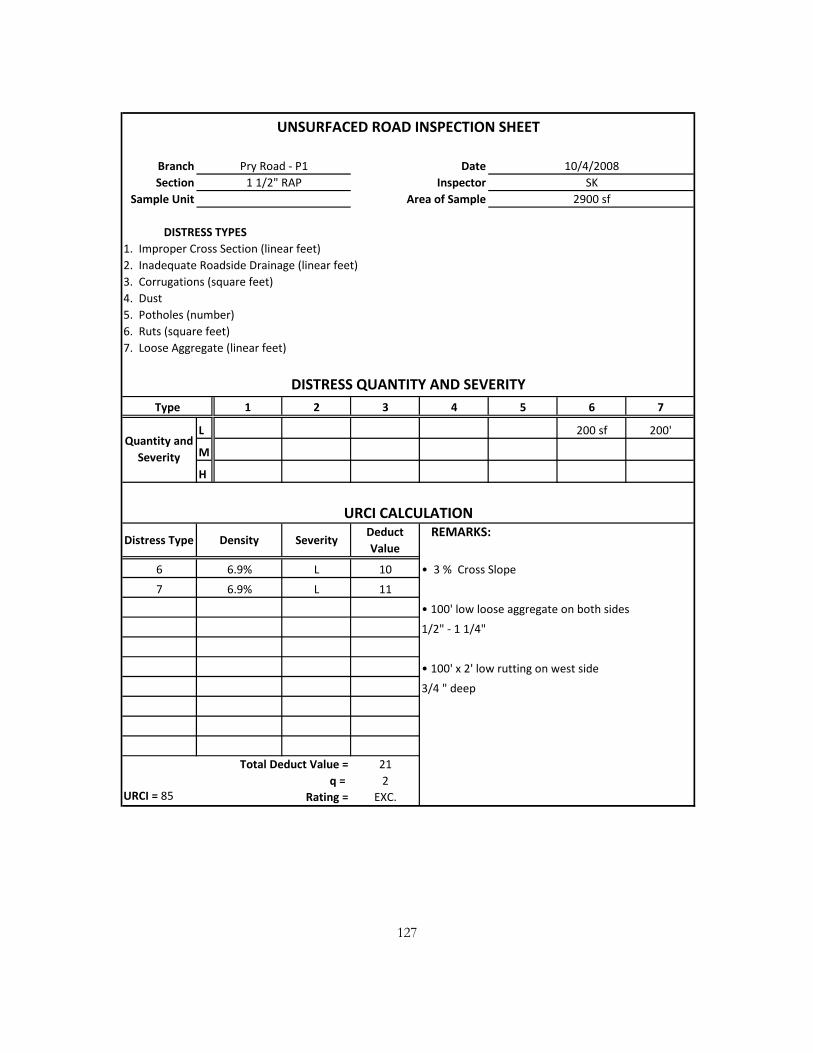
127

Branch DateSection Inspector

Sample Unit Area of Sample

DISTRESS TYPES1. Improper Cross Section (linear feet)2. Inadequate Roadside Drainage (linear feet)3. Corrugations (square feet)4. Dust5. Potholes (number)6. Ruts (square feet)7. Loose Aggregate (linear feet)

1 2 3 4 5 6 7

L 200 sf 200'

M

H

6 L 10 • 3 % Cross Slope

7 L 11

• 100' low loose aggregate on both sides

1/2" - 1 1/4"

• 100' x 2' low rutting on west side

3/4 " deep

Total Deduct Value = 21q = 2

URCI = 85 Rating = EXC.

UNSURFACED ROAD INSPECTION SHEET

Pry Road - P1 10/4/20081 1/2" RAP SK

2900 sf

DISTRESS QUANTITY AND SEVERITYType

Quantity and Severity

URCI CALCULATION

Distress Type Density SeverityDeduct Value

REMARKS:

6.9%

6.9%

128

Branch DateSection Inspector

Sample Unit Area of Sample

DISTRESS TYPES1. Improper Cross Section (linear feet)2. Inadequate Roadside Drainage (linear feet)3. Corrugations (square feet)4. Dust5. Potholes (number)6. Ruts (square feet)7. Loose Aggregate (linear feet)

1 2 3 4 5 6 7

L

M

H

• 2 % Cross Slope

• No Distresses

Total Deduct Value = 0q = 0

URCI = 100 Rating = EXC.

25' x 100 ' = 2500 sf

DISTRESS QUANTITY AND SEVERITYType

UNSURFACED ROAD INSPECTION SHEET

Pry Road - P0 6/24/2008

Quantity and Severity

URCI CALCULATION

Distress Type Density SeverityDeduct Value

REMARKS:

100% Gravel SK & GH

129

Branch DateSection Inspector

Sample Unit Area of Sample

DISTRESS TYPES1. Improper Cross Section (linear feet)2. Inadequate Roadside Drainage (linear feet)3. Corrugations (square feet)4. Dust5. Potholes (number)6. Ruts (square feet)7. Loose Aggregate (linear feet)

1 2 3 4 5 6 7

L

M

H

• 2 % Cross Slope

• No Distresses

Total Deduct Value = 0q = 0

URCI = 100 Rating = EXC.

Quantity and Severity

URCI CALCULATION

Distress Type Density SeverityDeduct Value

REMARKS:

100% Gravel SK2500 sf

DISTRESS QUANTITY AND SEVERITYType

UNSURFACED ROAD INSPECTION SHEET

Pry Road - P0 7/11/2008

130

Branch DateSection Inspector

Sample Unit Area of Sample

DISTRESS TYPES1. Improper Cross Section (linear feet)2. Inadequate Roadside Drainage (linear feet)3. Corrugations (square feet)4. Dust5. Potholes (number)6. Ruts (square feet)7. Loose Aggregate (linear feet)

1 2 3 4 5 6 7

L

M

H

• 2 % Cross Slope

• No Distresses

Total Deduct Value = 0q = 0

URCI = 100 Rating = EXC.

2500 sf

DISTRESS QUANTITY AND SEVERITYType

Quantity and Severity

UNSURFACED ROAD INSPECTION SHEET

Pry Road - P0 7/28/2008100% Gravel SK

URCI CALCULATION

Distress Type Density SeverityDeduct Value

REMARKS:

131

Branch DateSection Inspector

Sample Unit Area of Sample

DISTRESS TYPES1. Improper Cross Section (linear feet)2. Inadequate Roadside Drainage (linear feet)3. Corrugations (square feet)4. Dust5. Potholes (number)6. Ruts (square feet)7. Loose Aggregate (linear feet)

1 2 3 4 5 6 7

L

M

H

• 2 % Cross Slope

• No Distresses

Total Deduct Value = 0q = 0

URCI = 100 Rating = EXC.

2500 sf

DISTRESS QUANTITY AND SEVERITYType

Quantity and Severity

URCI CALCULATION

Distress Type Density SeverityDeduct Value

REMARKS:

UNSURFACED ROAD INSPECTION SHEET

Pry Road - P0 8/6/2008100% Gravel SK

132

Branch DateSection Inspector

Sample Unit Area of Sample

DISTRESS TYPES1. Improper Cross Section (linear feet)2. Inadequate Roadside Drainage (linear feet)3. Corrugations (square feet)4. Dust5. Potholes (number)6. Ruts (square feet)7. Loose Aggregate (linear feet)

1 2 3 4 5 6 7

L

M

H

• 2 % Cross Slope

• No Distresses

Total Deduct Value = 0q = 0

URCI = 100 Rating = EXC.

2500 sf

DISTRESS QUANTITY AND SEVERITYType

Quantity and Severity

URCI CALCULATION

Distress Type Density SeverityDeduct Value

REMARKS:

UNSURFACED ROAD INSPECTION SHEET

Pry Road - P0 8/13/2008100% Gravel SK

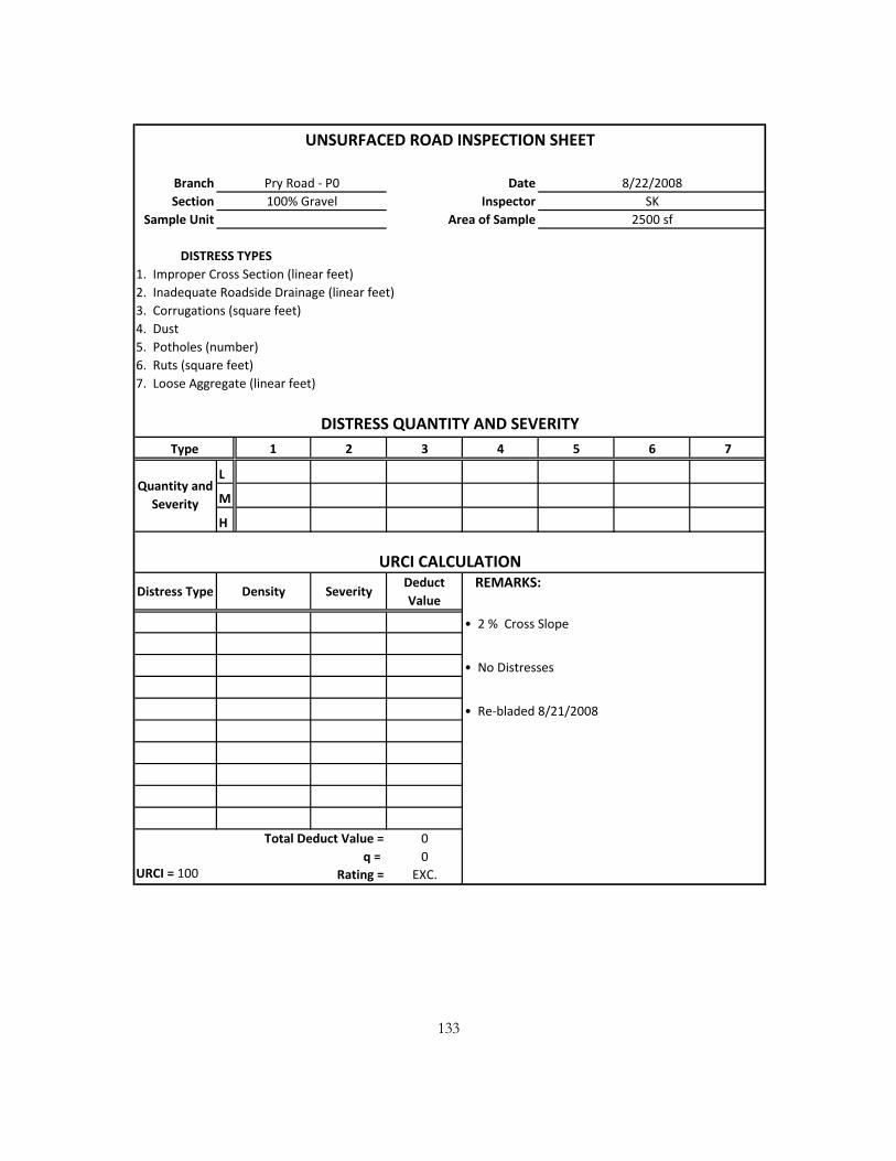
133

Branch DateSection Inspector

Sample Unit Area of Sample

DISTRESS TYPES1. Improper Cross Section (linear feet)2. Inadequate Roadside Drainage (linear feet)3. Corrugations (square feet)4. Dust5. Potholes (number)6. Ruts (square feet)7. Loose Aggregate (linear feet)

1 2 3 4 5 6 7

L

M

H

• 2 % Cross Slope

• No Distresses

• Re-bladed 8/21/2008

Total Deduct Value = 0q = 0

URCI = 100 Rating = EXC.

2500 sf

DISTRESS QUANTITY AND SEVERITYType

Quantity and Severity

URCI CALCULATION

Distress Type Density SeverityDeduct Value

REMARKS:

UNSURFACED ROAD INSPECTION SHEET

Pry Road - P0 8/22/2008100% Gravel SK

134

Branch DateSection Inspector

Sample Unit Area of Sample

DISTRESS TYPES1. Improper Cross Section (linear feet)2. Inadequate Roadside Drainage (linear feet)3. Corrugations (square feet)4. Dust5. Potholes (number)6. Ruts (square feet)7. Loose Aggregate (linear feet)

1 2 3 4 5 6 7

L

M

H

• 2 % Cross Slope

• No Distresses

Total Deduct Value = 0q = 0

URCI = 100 Rating = EXC.

UNSURFACED ROAD INSPECTION SHEET

Pry Road - P0 9/5/2008100% Gravel SK

2500 sf

DISTRESS QUANTITY AND SEVERITYType

Quantity and Severity

URCI CALCULATION

Distress Type Density SeverityDeduct Value

REMARKS:

135

Branch DateSection Inspector

Sample Unit Area of Sample

DISTRESS TYPES1. Improper Cross Section (linear feet)2. Inadequate Roadside Drainage (linear feet)3. Corrugations (square feet)4. Dust5. Potholes (number)6. Ruts (square feet)7. Loose Aggregate (linear feet)

1 2 3 4 5 6 7

L

M

H

• 2 % Cross Slope

• No Distresses

Total Deduct Value = 0q = 0

URCI = 100 Rating = EXC.

Type

Quantity and Severity

URCI CALCULATION

Distress Type Density SeverityDeduct Value

REMARKS:

UNSURFACED ROAD INSPECTION SHEET

Pry Road - P0 9/18/2008100% Gravel SK

2500 sf

DISTRESS QUANTITY AND SEVERITY

136

Branch DateSection Inspector

Sample Unit Area of Sample

DISTRESS TYPES1. Improper Cross Section (linear feet)2. Inadequate Roadside Drainage (linear feet)3. Corrugations (square feet)4. Dust5. Potholes (number)6. Ruts (square feet)7. Loose Aggregate (linear feet)

1 2 3 4 5 6 7

L

M

H

• 2 % Cross Slope

• No Distresses

Total Deduct Value = 0q = 0

URCI = 100 Rating = EXC.

UNSURFACED ROAD INSPECTION SHEET

Pry Road - P0 10/4/2008100% Gravel SK

2500 sf

DISTRESS QUANTITY AND SEVERITYType

Quantity and Severity

URCI CALCULATION

Distress Type Density SeverityDeduct Value

REMARKS:

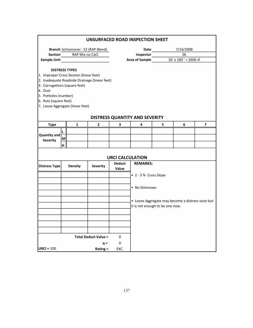
137

Branch Schoonover - S2 (RAP Blend) DateSection Inspector

Sample Unit Area of Sample

DISTRESS TYPES1. Improper Cross Section (linear feet)2. Inadequate Roadside Drainage (linear feet)3. Corrugations (square feet)4. Dust5. Potholes (number)6. Ruts (square feet)7. Loose Aggregate (linear feet)

1 2 3 4 5 6 7

L

M

H

• 2 - 3 % Cross Slope

• No Distresses

Total Deduct Value = 0

q = 0URCI = 100 Rating = EXC.

SK26' x 100 ' = 2600 sf

Distress Type Density SeverityDeduct Value

7/14/2008RAP Mix no CaCl

Quantity and Severity

Type

DISTRESS QUANTITY AND SEVERITY

REMARKS:URCI CALCULATION

• Loose Aggregate may become a distress soon but it is not enough to be one now.

UNSURFACED ROAD INSPECTION SHEET

138

Branch Schoonover - S2 (RAP Blend) DateSection Inspector

Sample Unit Area of Sample

DISTRESS TYPES1. Improper Cross Section (linear feet)2. Inadequate Roadside Drainage (linear feet)3. Corrugations (square feet)4. Dust5. Potholes (number)6. Ruts (square feet)7. Loose Aggregate (linear feet)

1 2 3 4 5 6 7

L 100 '

M

H

7 L 7 • 2 1/2 % Cross Slope

• 100' of Loose Aggregate on North Side

(Pic. 971).

1/2" - 1"

Total Deduct Value = 7

q = 1URCI = 95 Rating = EXC.

UNSURFACED ROAD INSPECTION SHEET

7/29/2008RAP Mix no CaCl SK

26' x 100 ' = 2600 sf

3.8%

DISTRESS QUANTITY AND SEVERITYType

Quantity and Severity

URCI CALCULATION

Distress Type Density SeverityDeduct Value

REMARKS:

139

Branch Schoonover - S2 (RAP Blend) DateSection Inspector

Sample Unit Area of Sample

DISTRESS TYPES1. Improper Cross Section (linear feet)2. Inadequate Roadside Drainage (linear feet)3. Corrugations (square feet)4. Dust5. Potholes (number)6. Ruts (square feet)7. Loose Aggregate (linear feet)

1 2 3 4 5 6 7

L 100 '

M

H

7 L 7 • 2 % Cross Slope

• 100' of Loose Aggregate on North Side

3/4" - 1"

Total Deduct Value = 7

q = 1URCI = 95 Rating = EXC.

Quantity and Severity

URCI CALCULATION

Distress Type Density SeverityDeduct Value

REMARKS:

3.8%

UNSURFACED ROAD INSPECTION SHEET

8/6/2008RAP Mix no CaCl SK

26' x 100 ' = 2600 sf

DISTRESS QUANTITY AND SEVERITYType

140

Branch Schoonover - S2 (RAP Blend) DateSection Inspector

Sample Unit Area of Sample

DISTRESS TYPES1. Improper Cross Section (linear feet)2. Inadequate Roadside Drainage (linear feet)3. Corrugations (square feet)4. Dust5. Potholes (number)6. Ruts (square feet)7. Loose Aggregate (linear feet)

1 2 3 4 5 6 7

L 100 '

M

H

7 L 7 • 2 % Cross Slope

• 100' of Loose Aggregate on North Side

Total Deduct Value = 7

q = 1URCI = 95 Rating = EXC.

UNSURFACED ROAD INSPECTION SHEET

8/13/2008RAP Mix no CaCl SK

26' x 100 ' = 2600 sf

DISTRESS QUANTITY AND SEVERITYType

Quantity and Severity

URCI CALCULATION

Distress Type Density SeverityDeduct Value

REMARKS:

3.8%

141

Branch Schoonover - S2 (RAP Blend) DateSection Inspector

Sample Unit Area of Sample

DISTRESS TYPES1. Improper Cross Section (linear feet)2. Inadequate Roadside Drainage (linear feet)3. Corrugations (square feet)4. Dust5. Potholes (number)6. Ruts (square feet)7. Loose Aggregate (linear feet)

1 2 3 4 5 6 7

L 140'

M

H

7 L 9 • 2 % Cross Slope

• 100' of Loose Aggregate on North Side

3/4" - 1 1/4"

• 40 ' of Loose Aggregate on South Side

1/2 " - 1"

Total Deduct Value = 9

q = 1URCI = 92 Rating = EXC.

UNSURFACED ROAD INSPECTION SHEET

8/21/2008RAP Mix no CaCl SK

26' x 100 ' = 2600 sf

DISTRESS QUANTITY AND SEVERITYType

Quantity and Severity

URCI CALCULATION

Distress Type Density SeverityDeduct Value

REMARKS:

5.4%

142

Branch Schoonover - S2 (RAP Blend) DateSection Inspector

Sample Unit Area of Sample

DISTRESS TYPES1. Improper Cross Section (linear feet)2. Inadequate Roadside Drainage (linear feet)3. Corrugations (square feet)4. Dust5. Potholes (number)6. Ruts (square feet)7. Loose Aggregate (linear feet)

1 2 3 4 5 6 7

L 160'

M

H

7 L 11 • 2 % Cross Slope

• 100' of Loose Aggregate on North Side

3/4" - 1 1/4"

• 60 ' of Loose Aggregate on South Side

1/2 " - 1"

Total Deduct Value = 11

q = 1URCI = 90 Rating = EXC.

UNSURFACED ROAD INSPECTION SHEET

9/1/2008RAP Mix no CaCl SK

26' x 100 ' = 2600 sf

DISTRESS QUANTITY AND SEVERITYType

Quantity and Severity

URCI CALCULATION

Distress Type Density SeverityDeduct Value

REMARKS:

6.2%

143

Branch Schoonover - S2 (RAP Blend) DateSection Inspector

Sample Unit Area of Sample

DISTRESS TYPES1. Improper Cross Section (linear feet)2. Inadequate Roadside Drainage (linear feet)3. Corrugations (square feet)4. Dust5. Potholes (number)6. Ruts (square feet)7. Loose Aggregate (linear feet)

1 2 3 4 5 6 7

L 200'

M

H

7 L 12 • 2 % Cross Slope

• 100' of Loose Aggregate on North Side

3/4" - 1 1/4"

• 100 ' of Loose Aggregate on South Side

1/2 " - 1 1/2"

Total Deduct Value = 12

q = 1URCI = 88 Rating = EXC.

UNSURFACED ROAD INSPECTION SHEET

10/4/2008RAP Mix no CaCl SK

26' x 100 ' = 2600 sf

DISTRESS QUANTITY AND SEVERITYType

Quantity and Severity

URCI CALCULATION

Distress Type Density SeverityDeduct Value

REMARKS:

7.7%

144

Branch Schoonover - S1 (RAP Blend w/ CaCl) DateSection Inspector

Sample Unit Area of Sample

DISTRESS TYPES1. Improper Cross Section (linear feet)2. Inadequate Roadside Drainage (linear feet)3. Corrugations (square feet)4. Dust5. Potholes (number)6. Ruts (square feet)7. Loose Aggregate (linear feet)

1 2 3 4 5 6 7

L

M

H

• 2 % Cross Slope

• No Distresses

• Potential for rutting

Total Deduct Value = 0q = 0

URCI = 100 Rating = EXC.

Distress Type Density SeverityDeduct Value

REMARKS:

27' x 100 ' = 2700 sf

DISTRESS QUANTITY AND SEVERITYType

Quantity and Severity

URCI CALCULATION

UNSURFACED ROAD INSPECTION SHEET

7/14/2008RAP Mix with CaCl SK

145

Branch Schoonover - S1 (RAP Blend w/ CaCl) DateSection Inspector

Sample Unit Area of Sample

DISTRESS TYPES1. Improper Cross Section (linear feet)2. Inadequate Roadside Drainage (linear feet)3. Corrugations (square feet)4. Dust5. Potholes (number)6. Ruts (square feet)7. Loose Aggregate (linear feet)

1 2 3 4 5 6 7

L

M

H

• 2 % Cross Slope

• No Distresses

• Potential for rutting in future

Total Deduct Value = 0q = 0

URCI = 100 Rating = EXC.

UNSURFACED ROAD INSPECTION SHEET

7/29/2008RAP Mix with CaCl SK

27' x 100 ' = 2700 sf

DISTRESS QUANTITY AND SEVERITYType

Quantity and Severity

URCI CALCULATION

Distress Type Density SeverityDeduct Value

REMARKS:

• Potential Loose Aggregate on South Side in future

146

Branch Schoonover - S1 (RAP Blend w/ CaCl) DateSection Inspector

Sample Unit Area of Sample

DISTRESS TYPES1. Improper Cross Section (linear feet)2. Inadequate Roadside Drainage (linear feet)3. Corrugations (square feet)4. Dust5. Potholes (number)6. Ruts (square feet)7. Loose Aggregate (linear feet)

1 2 3 4 5 6 7

L 150 sf 30 '

M

H

7 L 2 • 2 % Cross Slope

6 L 8

• 50 ' of Low rutting on south side

50' x 3' = 150 sf

• 30' of Loose Aggregate on south side

1/2" - 3/4 "

Total Deduct Value = 10q = 1

URCI = 90 Rating = EXC.

URCI CALCULATION

Distress Type Density SeverityDeduct Value

REMARKS:

1.1%

5.5%

8/6/2008RAP Mix with CaCl SK

27' x 100 ' = 2700 sf

DISTRESS QUANTITY AND SEVERITYType

Quantity and Severity

UNSURFACED ROAD INSPECTION SHEET

147

Branch Schoonover - S1 (RAP Blend w/ CaCl) DateSection Inspector

Sample Unit Area of Sample

DISTRESS TYPES1. Improper Cross Section (linear feet)2. Inadequate Roadside Drainage (linear feet)3. Corrugations (square feet)4. Dust5. Potholes (number)6. Ruts (square feet)7. Loose Aggregate (linear feet)

1 2 3 4 5 6 7

L 150 sf 50'

M

H

6 L 8 • 2 % Cross Slope

7 L 4

• 50 ' of Low rutting on south side

50' x 3' = 150 sf

• 50' of Loose Aggregate on south side

1/2" - 3/4 "

Total Deduct Value = 12q = 1

URCI = 87 Rating = EXC.

Quantity and Severity

URCI CALCULATION

Distress Type Density SeverityDeduct Value

REMARKS:

5.5%

1.8%

UNSURFACED ROAD INSPECTION SHEET

8/13/2008RAP Mix with CaCl SK

27' x 100 ' = 2700 sf

DISTRESS QUANTITY AND SEVERITYType

148

Branch Schoonover - S1 (RAP Blend w/ CaCl) DateSection Inspector

Sample Unit Area of Sample

DISTRESS TYPES1. Improper Cross Section (linear feet)2. Inadequate Roadside Drainage (linear feet)3. Corrugations (square feet)4. Dust5. Potholes (number)6. Ruts (square feet)7. Loose Aggregate (linear feet)

1 2 3 4 5 6 7

L 225 sf 100'

M

H

6 L 12 • 2 % Cross Slope

7 L 7

• 75 ' of Low rutting on south side

75' x 3' = 225 sf

• 100' of Loose Aggregate on south side

1/2" - 1"

Total Deduct Value = 19q = 2

URCI = 87 Rating = EXC.

UNSURFACED ROAD INSPECTION SHEET

8/21/2008RAP Mix with CaCl SK

27' x 100 ' = 2700 sf

DISTRESS QUANTITY AND SEVERITYType

Quantity and Severity

URCI CALCULATION

Distress Type Density SeverityDeduct Value

REMARKS:

8.3%

3.7%

149

Branch Schoonover - S1 (RAP Blend w/ CaCl) DateSection Inspector

Sample Unit Area of Sample

DISTRESS TYPES1. Improper Cross Section (linear feet)2. Inadequate Roadside Drainage (linear feet)3. Corrugations (square feet)4. Dust5. Potholes (number)6. Ruts (square feet)7. Loose Aggregate (linear feet)

1 2 3 4 5 6 7

L 225 sf 125'

M

H

6 L 12 • 2 % Cross Slope

7 L 9

• 75 ' of Low rutting on south side

75' x 3' = 225 sf

• 100' of Loose Aggregate on south side

1/2" - 1"

• 25' of Loose Aggregate on north side

1/2" - 3/4"Total Deduct Value = 21

q = 2URCI = 84 Rating = EXC.

URCI CALCULATION

Distress Type Density SeverityDeduct Value

REMARKS:

8.3%

4.6%

9/1/2008RAP Mix with CaCl SK

27' x 100 ' = 2700 sf

DISTRESS QUANTITY AND SEVERITYType

Quantity and Severity

UNSURFACED ROAD INSPECTION SHEET

150

Branch Schoonover - S1 (RAP Blend w/ CaCl) DateSection Inspector

Sample Unit Area of Sample

DISTRESS TYPES1. Improper Cross Section (linear feet)2. Inadequate Roadside Drainage (linear feet)3. Corrugations (square feet)4. Dust5. Potholes (number)6. Ruts (square feet)7. Loose Aggregate (linear feet)

1 2 3 4 5 6 7

L 135 sf 140'

M

H

6 L 9 • 2 % Cross Slope

7 L 9

• 45 ' of Low rutting on south side

75' x 3' = 135 sf

• 100' of Loose Aggregate on south side

1/2" - 1"

• 40' of Loose Aggregate on north side

1/2" - 3/4"Total Deduct Value = 17

q = 2URCI = 88 Rating = EXC.

UNSURFACED ROAD INSPECTION SHEET

10/4/2008RAP Mix with CaCl SK

27' x 100 ' = 2700 sf

DISTRESS QUANTITY AND SEVERITYType

Quantity and Severity

URCI CALCULATION

Distress Type Density SeverityDeduct Value

REMARKS:

5.0%

5.2%

151

Branch Schoonover - S0 (100% Gravel w/ CaCl) DateSection Inspector

Sample Unit Area of Sample

DISTRESS TYPES1. Improper Cross Section (linear feet)2. Inadequate Roadside Drainage (linear feet)3. Corrugations (square feet)4. Dust5. Potholes (number)6. Ruts (square feet)7. Loose Aggregate (linear feet)

1 2 3 4 5 6 7

L

M

H

• 2 % Cross Slope

• No Distresses

• Potential for rutting

Total Deduct Value = 0q = 0

URCI = 100 Rating = EXC.

7/14/2008Gravel with CaCl SK

UNSURFACED ROAD INSPECTION SHEET

Type

Quantity and Severity

URCI CALCULATION

27' x 100 ' = 2700 sf

DISTRESS QUANTITY AND SEVERITY

Distress Type Density SeverityDeduct Value

REMARKS:

152

Branch Schoonover - S0 (100% Gravel w/ CaCl) DateSection Inspector

Sample Unit Area of Sample

DISTRESS TYPES1. Improper Cross Section (linear feet)2. Inadequate Roadside Drainage (linear feet)3. Corrugations (square feet)4. Dust5. Potholes (number)6. Ruts (square feet)7. Loose Aggregate (linear feet)

1 2 3 4 5 6 7

L 100 sf

M

H

6 L 4 • 2 % Cross Slope

• 1' x 100' Rutting. Small but noticeable

(Pic. 967, 968)

Total Deduct Value = 4q = 0

URCI = 97 Rating = EXC.

7/29/2008Gravel with CaCl SK

UNSURFACED ROAD INSPECTION SHEET

Type

Quantity and Severity

URCI CALCULATION

27' x 100 ' = 2700 sf

DISTRESS QUANTITY AND SEVERITY

REMARKS:

3.7%

Distress Type Density SeverityDeduct Value

153

Branch Schoonover - S0 (100% Gravel w/ CaCl) DateSection Inspector

Sample Unit Area of Sample

DISTRESS TYPES1. Improper Cross Section (linear feet)2. Inadequate Roadside Drainage (linear feet)3. Corrugations (square feet)4. Dust5. Potholes (number)6. Ruts (square feet)7. Loose Aggregate (linear feet)

1 2 3 4 5 6 7

L 100 sf 120'

M

H

6 L 5 • 2 % Cross Slope

7 L 8

• 1' x 100' Rutting down centerline

1 " deep

• 100' of Loose Aggregate on south side

3/4" - 1 1/2 "

• 20' of Loose Aggregate on north side

1/2" - 1"Total Deduct Value = 13

q = 2URCI = 90 Rating = EXC.

URCI CALCULATION

Distress Type Density SeverityDeduct Value

REMARKS:

3.7%

4.4%

8/6/2008Gravel with CaCl SK

27' x 100 ' = 2700 sf

DISTRESS QUANTITY AND SEVERITYType

Quantity and Severity

UNSURFACED ROAD INSPECTION SHEET

154

Branch Schoonover - S0 (100% Gravel w/ CaCl) DateSection Inspector

Sample Unit Area of Sample

DISTRESS TYPES1. Improper Cross Section (linear feet)2. Inadequate Roadside Drainage (linear feet)3. Corrugations (square feet)4. Dust5. Potholes (number)6. Ruts (square feet)7. Loose Aggregate (linear feet)

1 2 3 4 5 6 7

L

M

H

• no inspection recorded

Total Deduct Value =q =

URCI = Rating =

Gravel with CaCl SK27' x 100 ' = 2700 sf

DISTRESS QUANTITY AND SEVERITYType

Quantity and Severity

URCI CALCULATION

Distress Type Density SeverityDeduct Value

REMARKS:

UNSURFACED ROAD INSPECTION SHEET

8/13/2008

155

Branch Schoonover - S0 (100% Gravel w/ CaCl) DateSection Inspector

Sample Unit Area of Sample

DISTRESS TYPES1. Improper Cross Section (linear feet)2. Inadequate Roadside Drainage (linear feet)3. Corrugations (square feet)4. Dust5. Potholes (number)6. Ruts (square feet)7. Loose Aggregate (linear feet)

1 2 3 4 5 6 7

L 200 sf 150'

M

H

6 L 10 • 2 % Cross Slope

7 L 10

• 2' x 100' Low Rutting down centerline

1 " deep

• 50' of Loose Aggregate on south side

1/2" - 3/4"

• 100' of Loose Aggregate on north side

1/2" - 1"Total Deduct Value = 20

q = 2URCI = 85 Rating = EXC.

5.6%

7.4%

Quantity and Severity

URCI CALCULATION

Distress Type Density SeverityDeduct Value

REMARKS:

UNSURFACED ROAD INSPECTION SHEET

8/21/2008Gravel with CaCl SK

27' x 100 ' = 2700 sf

DISTRESS QUANTITY AND SEVERITYType

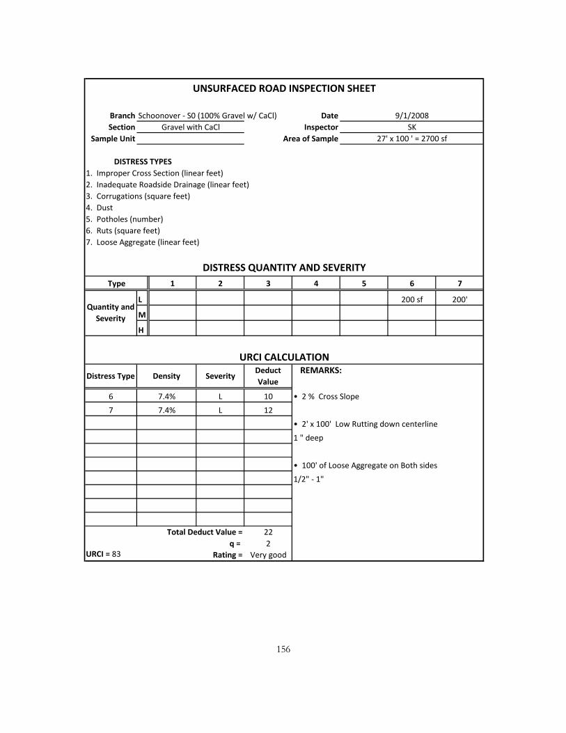
156

Branch Schoonover - S0 (100% Gravel w/ CaCl) DateSection Inspector

Sample Unit Area of Sample

DISTRESS TYPES1. Improper Cross Section (linear feet)2. Inadequate Roadside Drainage (linear feet)3. Corrugations (square feet)4. Dust5. Potholes (number)6. Ruts (square feet)7. Loose Aggregate (linear feet)

1 2 3 4 5 6 7

L 200 sf 200'

M

H

6 L 10 • 2 % Cross Slope

7 L 12

• 2' x 100' Low Rutting down centerline

1 " deep

• 100' of Loose Aggregate on Both sides

1/2" - 1"

Total Deduct Value = 22q = 2

URCI = 83 Rating = Very good

7.4%

UNSURFACED ROAD INSPECTION SHEET

9/1/2008Gravel with CaCl

DISTRESS QUANTITY AND SEVERITYType

Quantity and Severity

URCI CALCULATION

Distress Type Density SeverityDeduct Value

REMARKS:

7.4%

SK27' x 100 ' = 2700 sf

157

Branch Schoonover - S0 (100% Gravel w/ CaCl) DateSection Inspector

Sample Unit Area of Sample

DISTRESS TYPES1. Improper Cross Section (linear feet)2. Inadequate Roadside Drainage (linear feet)3. Corrugations (square feet)4. Dust5. Potholes (number)6. Ruts (square feet)7. Loose Aggregate (linear feet)

1 2 3 4 5 6 7

L 1400 sf 300 sf 200'

M 200 sf

H

3 L 24 • 2 % Cross Slope

6 L 15

6 M 14 • 2' x 100' Medium Rutting down centerline

7 L 12 1 1/2 " deep

• 100' of Loose Aggregate on Both sides

1/2" - 1"

• 100' x 3' low rutting on south side

1/2" - 1" deepTotal Deduct Value = 65

q = 4 • < 1" corrugations centered on centerlineURCI = 65 Rating = good 100' x 14'

UNSURFACED ROAD INSPECTION SHEET

10/4/2008Gravel with CaCl SK

27' x 100 ' = 2700 sf

DISTRESS QUANTITY AND SEVERITYType

Quantity and Severity

URCI CALCULATION

Distress Type Density SeverityDeduct Value

REMARKS:

51.9%

11.1%

7.4

7.4

158

159

APPENDIX C MATERIAL TESTING DATA SHEETS

160

161

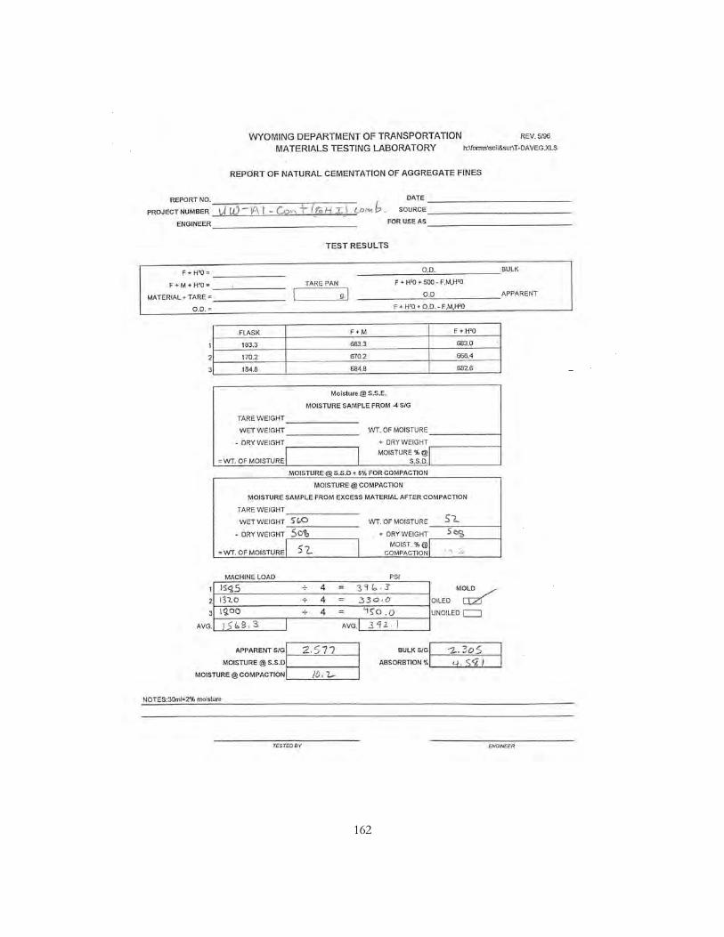
162

163

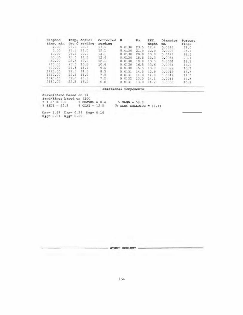
164

165

166

167

168

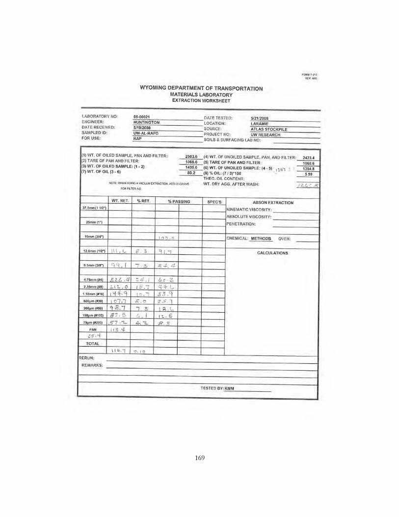
169

170

171

172

173

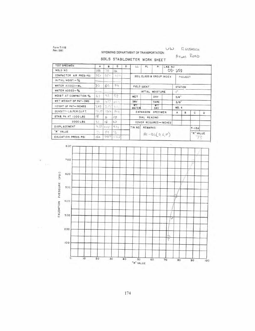
174

175

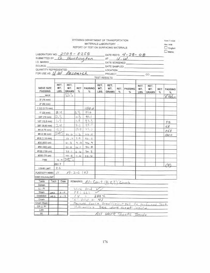
176

177

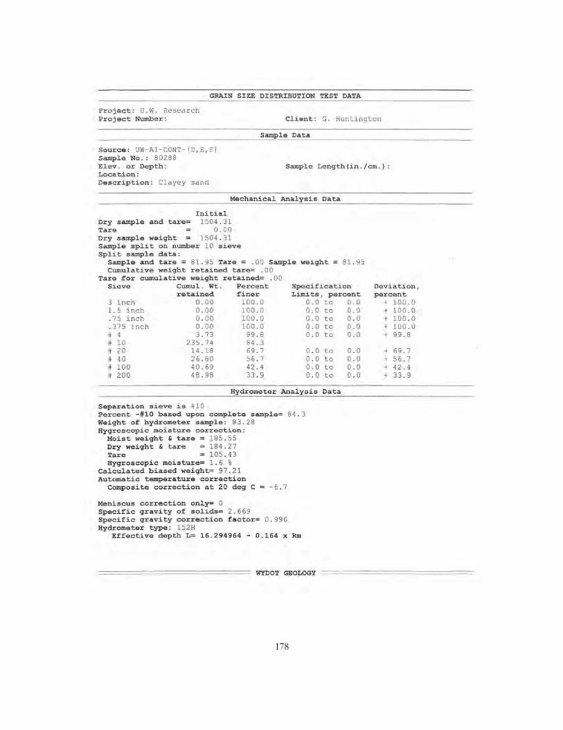
178

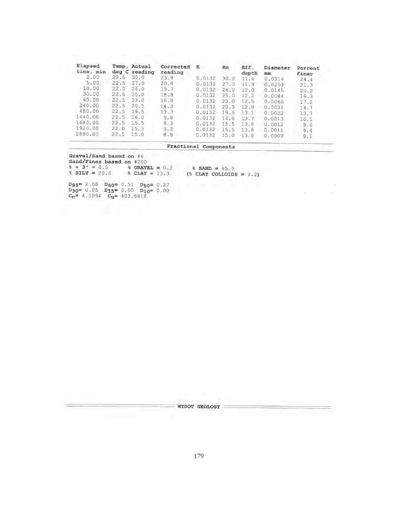
179

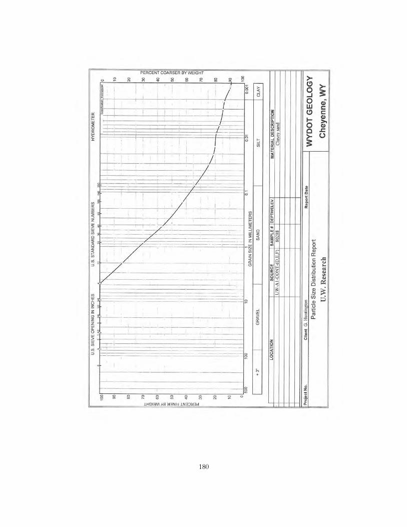
180

181

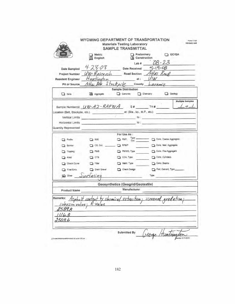
182

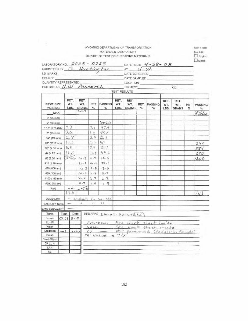
183

184

185

186

187

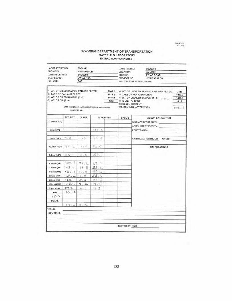
188

189

190

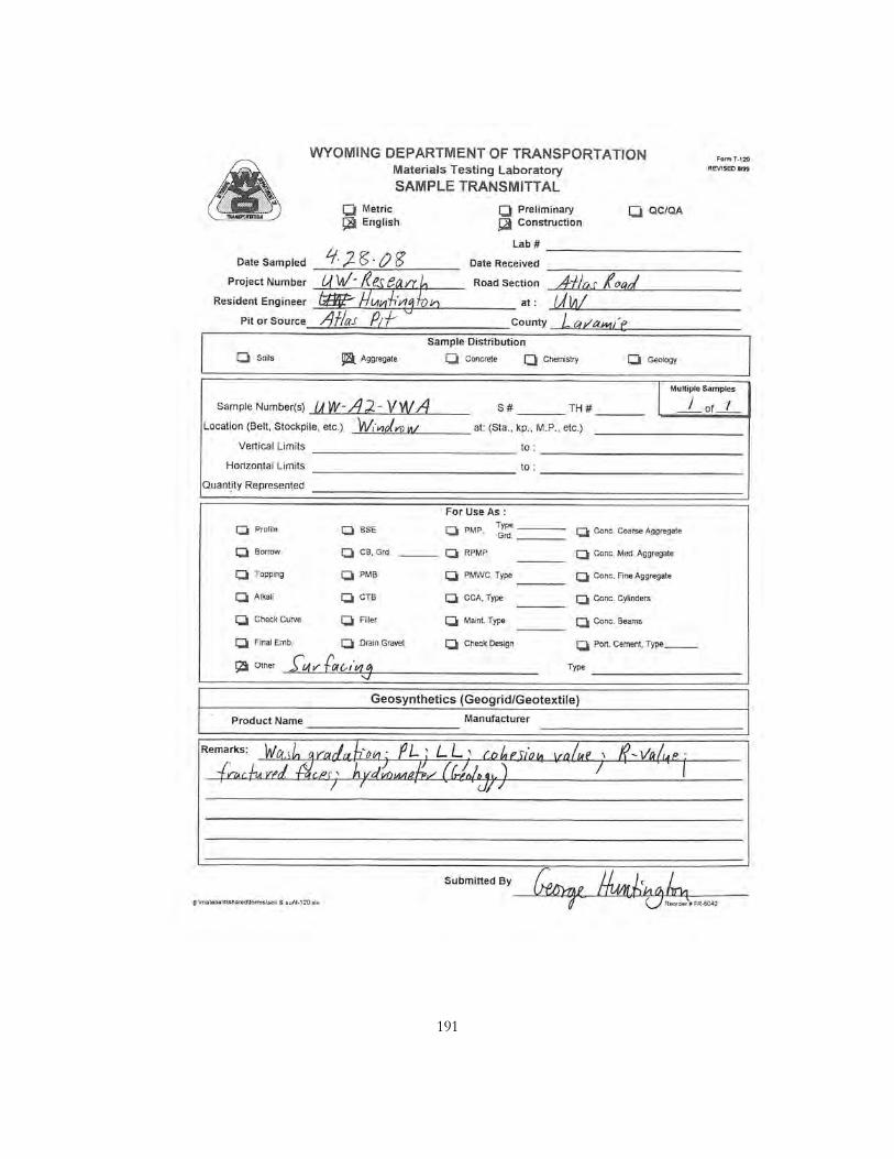
191

192

193

194

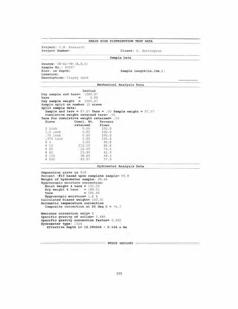
195

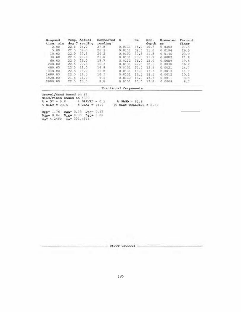
196

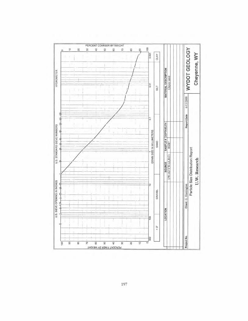
197

198

199

200

201

202

203

204

205

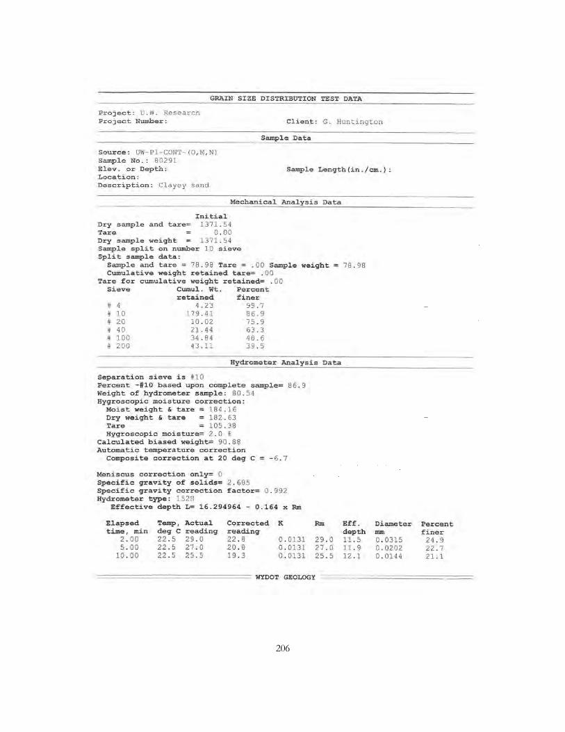
206

207

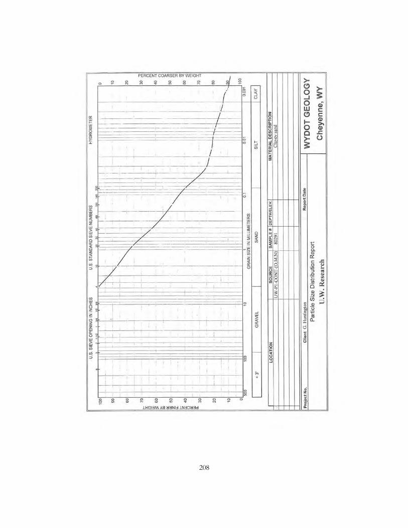
208

209

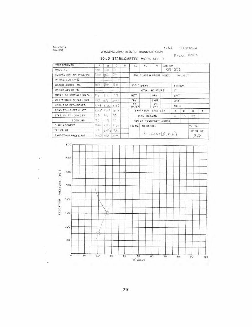
210

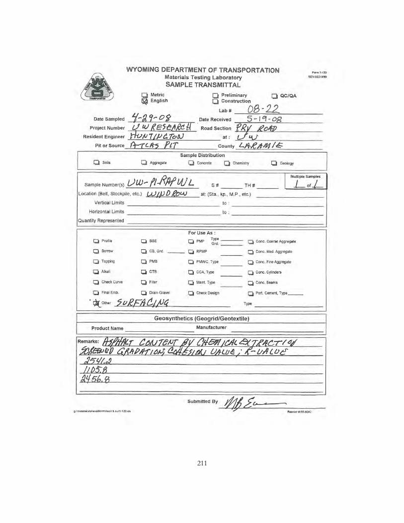
211

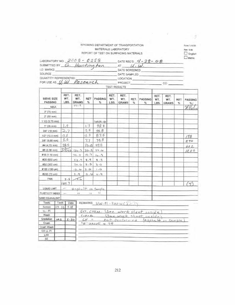
212

213

214

215

216

217

218

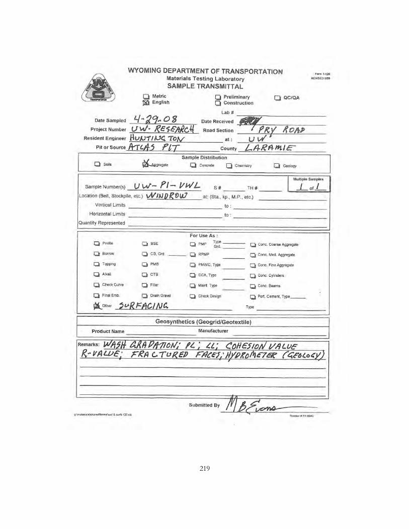
219

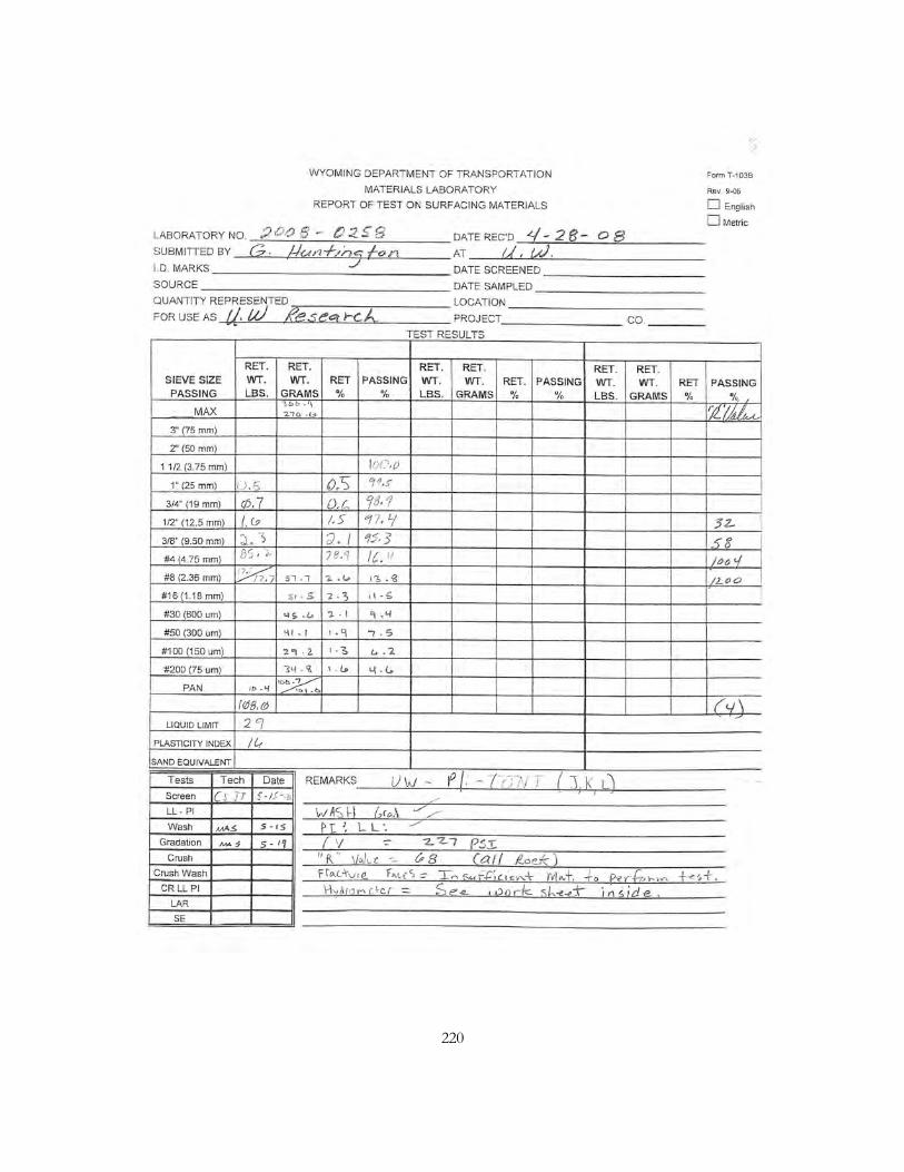
220

221

222

223

224

225

226

227

228

229

230

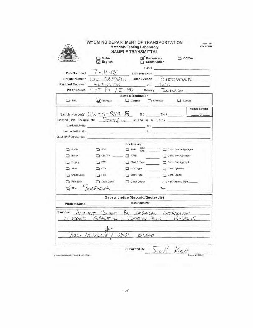
231

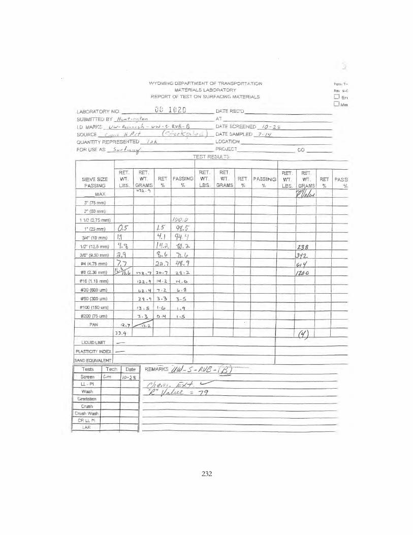
232

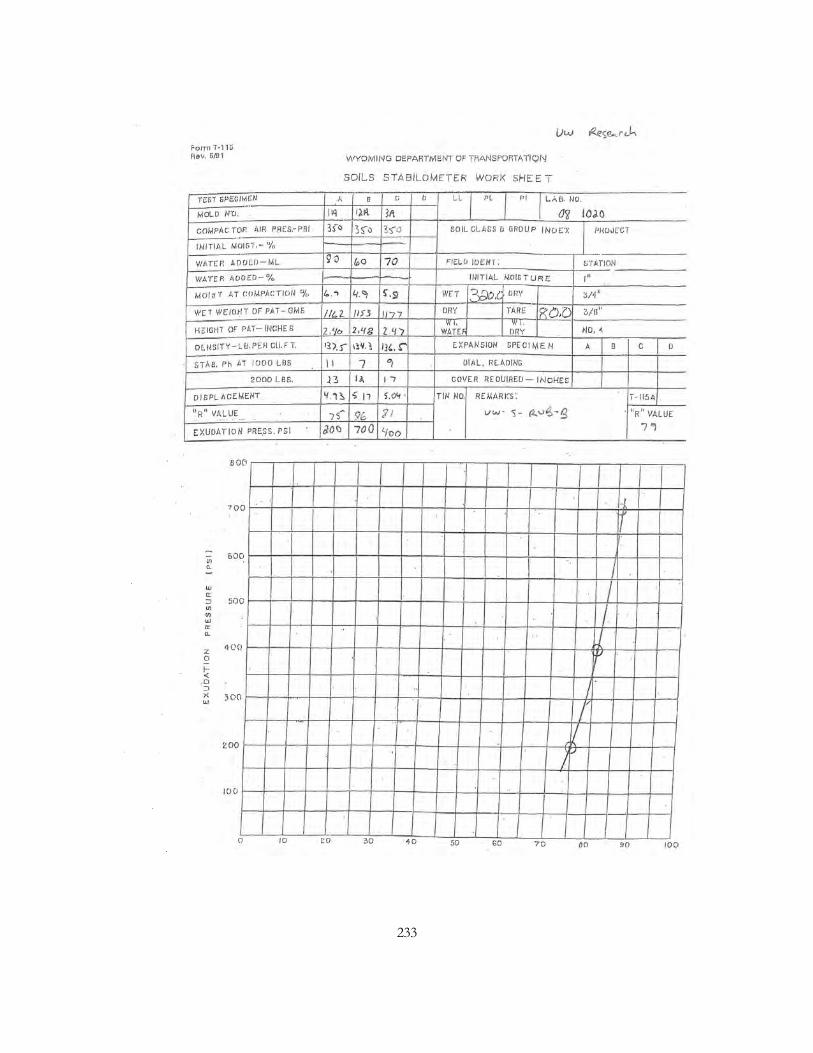
233

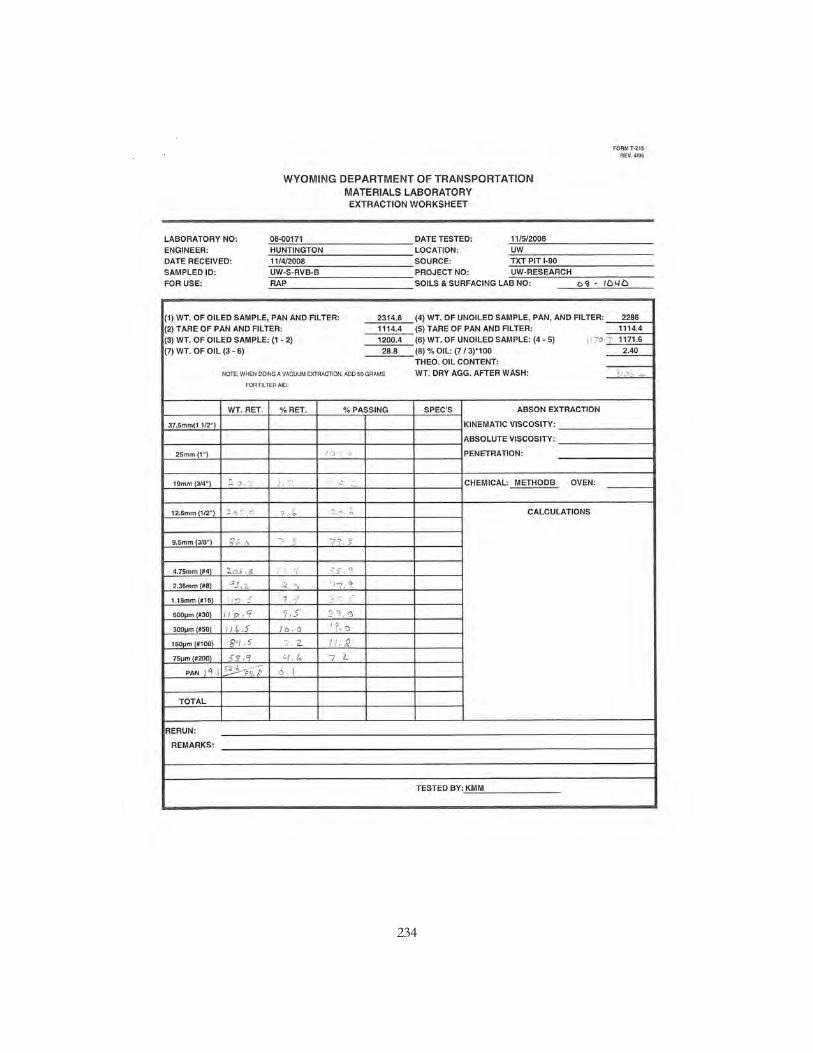
234

235

236

237

238

239

240

241

242

243

244

245

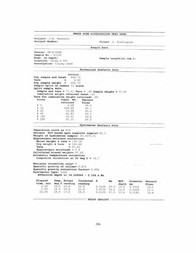
246

247

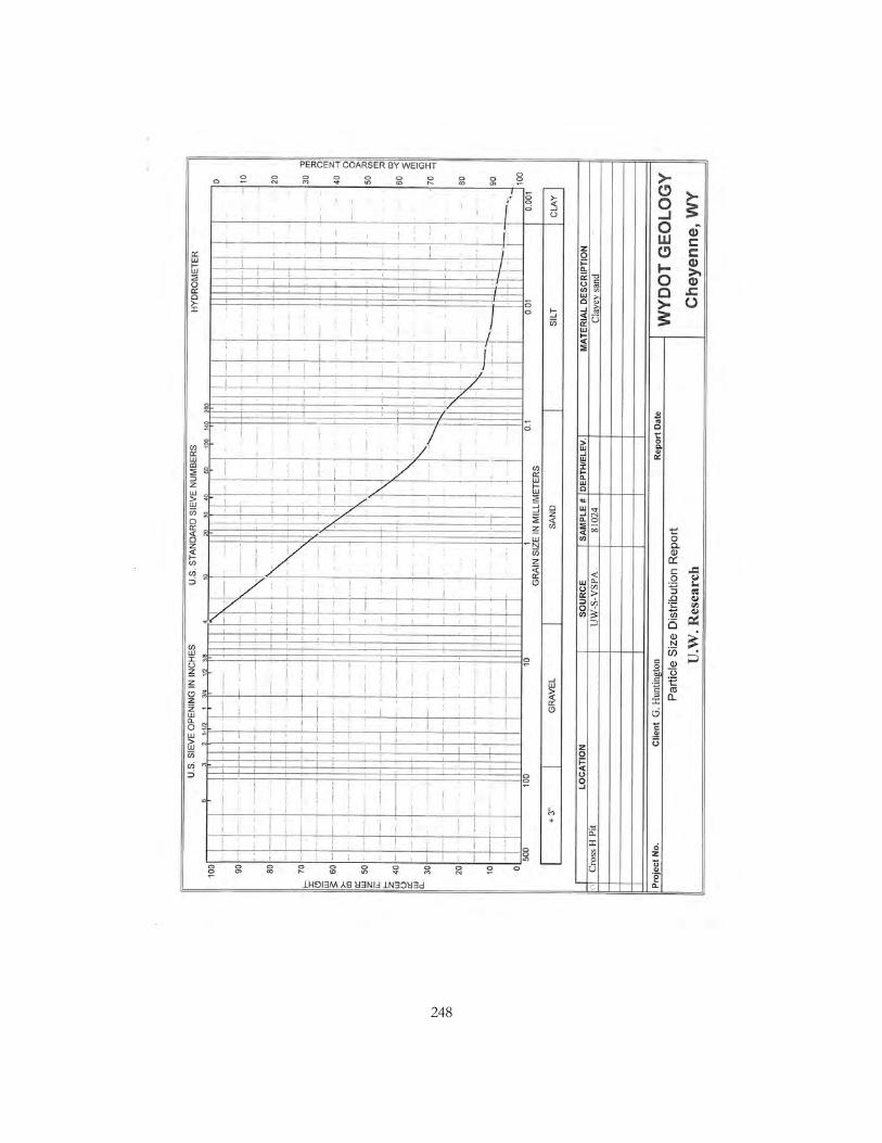
248

249

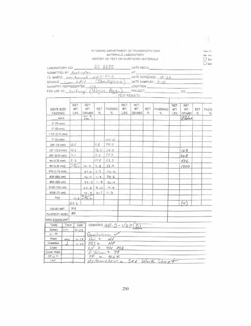
250

251

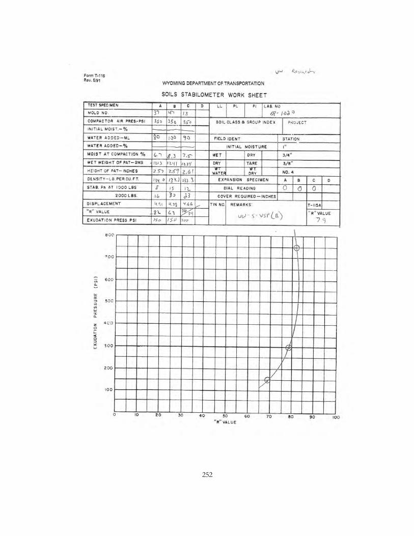
252

253

254

255

256

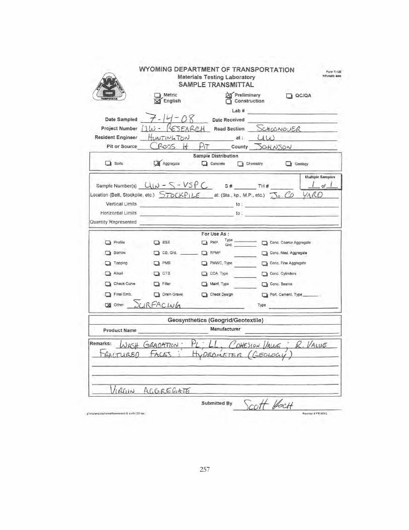
257

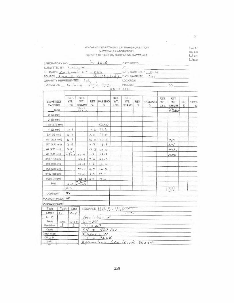
258

259

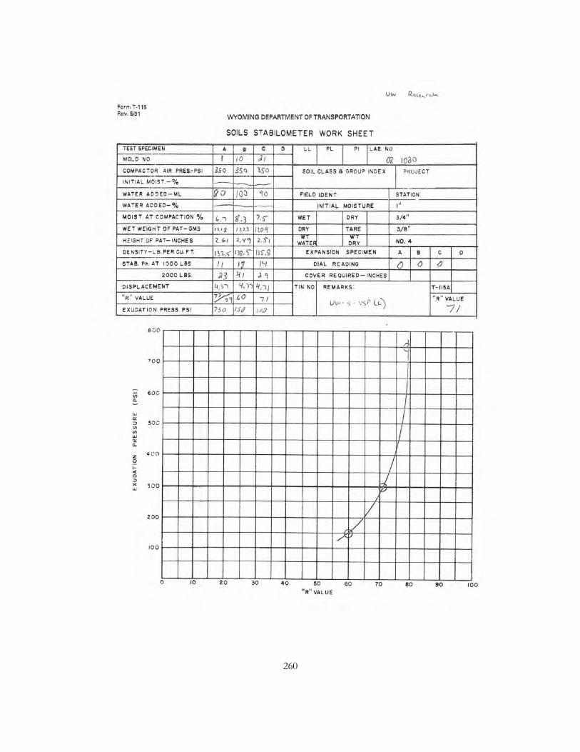
260

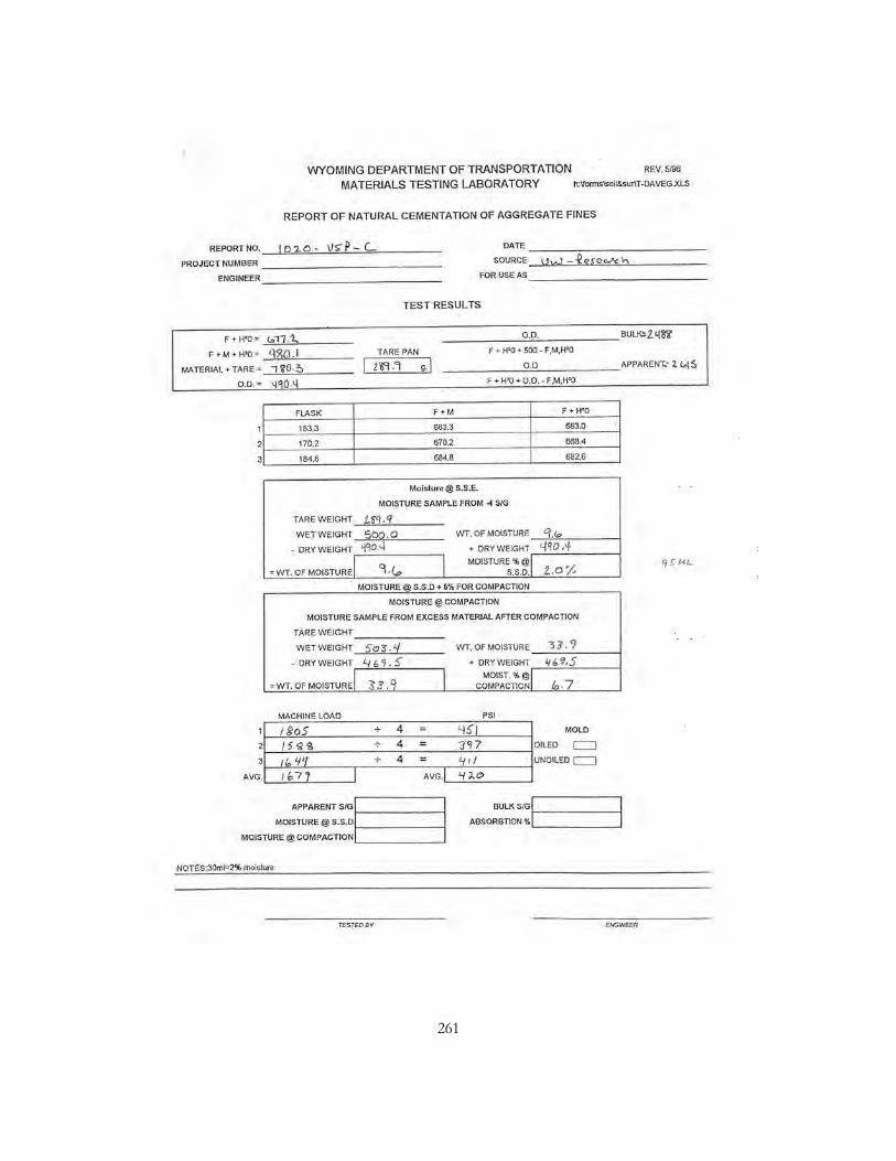
261

262

263

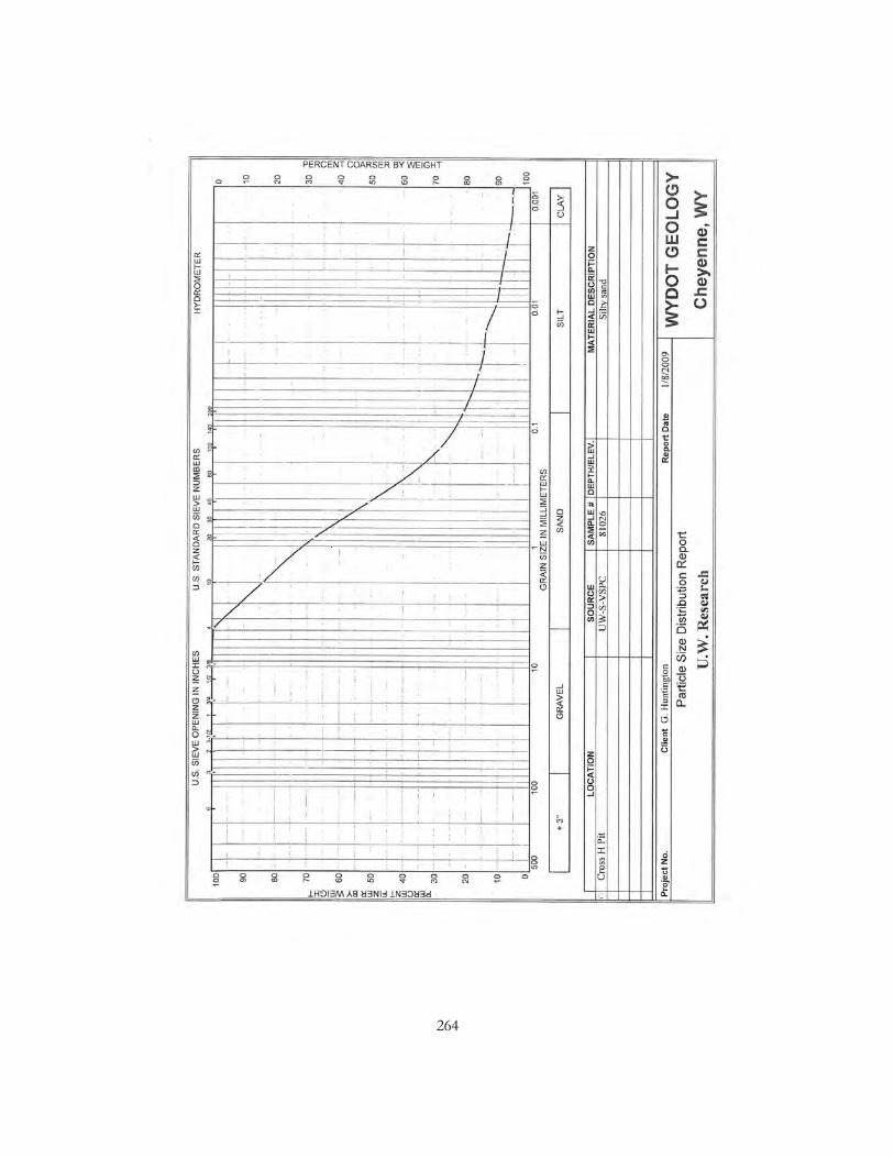
264

265

APPENDIX D SAS CODE AND RESULTS

266

SAS Code for Dust Contrasts

DM LOG 'CLEAR'; DM OUTPUT 'CLEAR'; DATA Both_Counties_Average; INFILE 'R:\RAP Writings & Data\DATA\Statistical Analysis\Both Counties SAS\Average.csv' DLM = ',' DSD MISSOVER; INPUT Section $ Dust Moisture Age Wind Pass; Log_Dust=log(Dust); PROC PRINT DATA = Both_Counties_Average; TITLE 'Estimate No Pass Both Counties Average' ; RUN; ODS RTF FILE = 'R:\RAP Writings & Data\DATA\Statistical Analysis\Both Counties SAS\Estimate No Pass Both Counties Average.rtf' BODYTITLE; PROC GLM alpha = 0.10 DATA=Both_Counties_Average; CLASS Section; MODEL Log_Dust = Section Moisture Age Wind /solution; ESTIMATE 'Average Laramie vs Johnson' section 3 3 3 3 3 -5 -5 -5/ DIVISOR=15; ESTIMATE 'Average noRAP vs RAP' section 5 -3 -3 5 -3 5 -3 -3/ DIVISOR=15; ESTIMATE 'Average noCaCl vs CaCl' section 1 1 1 1 1 -3 -3 1/ DIVISOR=6; output p=fit r=res out=datsec; RUN; ODS RTF CLOSE;

267

SAS Code for URCI Contrasts

DM LOG 'CLEAR'; DM OUTPUT 'CLEAR'; DATA Both_Counties_Average_URCI; INFILE 'R:\RAP Writings & Data\DATA\Statistical Analysis\Both Counties SAS\AverageWithURCI.csv' DLM = ',' DSD MISSOVER; INPUT Section $ URCI Dust Moisture Age Wind Pass; PROC PRINT DATA = Both_Counties_Average_URCI; TITLE 'Estimate No Pass Both Counties Average URCI' ; RUN; ODS RTF FILE = 'R:\RAP Writings & Data\DATA\Statistical Analysis\Both Counties SAS\Estimate No Pass Both Counties Average URCI.rtf' BODYTITLE; PROC GLM alpha = 0.10 DATA=Both_Counties_Average_URCI; CLASS Section; MODEL URCI = Section Dust Moisture Age Wind /solution; ESTIMATE 'Average URCI Laramie vs Johnson' section 3 3 3 3 3 -5 -5 -5/ DIVISOR=15; ESTIMATE 'Average URCI noRAP vs RAP' section 5 -3 -3 5 -3 5 -3 -3/ DIVISOR=15; ESTIMATE 'Average URCI noCaCl vs CaCl' section 1 1 1 1 1 -3 -3 1/ DIVISOR=6; output p=fit r=res out=datsec; RUN; ODS RTF CLOSE;

268

SAS Results for Average Contrasts

Estimate Both Counties Average

The GLM Procedure

Class Level Information

Class Levels Values

Section 8 A0 A1 A2 P0 P1 S0 S1 S2

Number of Observations Read 96

Number of Observations Used 95

The GLM Procedure

Dependent Variable: Log_Dust

Source DF Sum of

Squares Mean Square F Value Pr > F

Model 10 35.96941872 3.59694187 10.34 <.0001

Error 84 29.22510617 0.34791793

Corrected Total 94 65.19452489

269

R-Square Coeff Var Root MSE Log_Dust Mean

0.551725 -123.8379 0.589846 -0.476305

Source DF Type I SS Mean Square F Value Pr > F

Section 7 16.40863705 2.34409101 6.74 <.0001

Moisture 1 0.18007628 0.18007628 0.52 0.4739

Age 1 10.56048849 10.56048849 30.35 <.0001

Wind 1 8.82021690 8.82021690 25.35 <.0001

Source DF Type III SS Mean Square F Value Pr > F

Section 7 28.53127923 4.07589703 11.72 <.0001

Moisture 1 0.10082701 0.10082701 0.29 0.5918

Age 1 7.93235049 7.93235049 22.80 <.0001

Wind 1 8.82021690 8.82021690 25.35 <.0001

270

Parameter Estimate Standard Error t Value Pr > |t|

Average Laramie vs Johnson 1.05741117 0.13723690 7.71 <.0001

Average noRAP vs RAP 0.38804705 0.13641207 2.84 0.0056

Average noCaCl vs CaCl 1.26457298 0.16427895 7.70 <.0001

Parameter Estimate Standard Error t Value Pr > |t|

Intercept 0.218606698 B 0.20751041 1.05 0.2951

Section A0 0.615692996 B 0.24718199 2.49 0.0147

Section A1 0.284570246 B 0.23352320 1.22 0.2264

Section A2 0.374399685 B 0.23112192 1.62 0.1090

Section P0 0.800149550 B 0.24199452 3.31 0.0014

Section P1 0.336765895 B 0.23837916 1.41 0.1614

Section S0 -0.430894872 B 0.26174894 -1.65 0.1035

Section S1 -1.294391623 B 0.25694116 -5.04 <.0001

Section S2 0.000000000 B . . .

Moisture 0.047883216 0.08894740 0.54 0.5918

Age -0.009349600 0.00195808 -4.77 <.0001

Wind -0.074204682 0.01473771 -5.04 <.0001

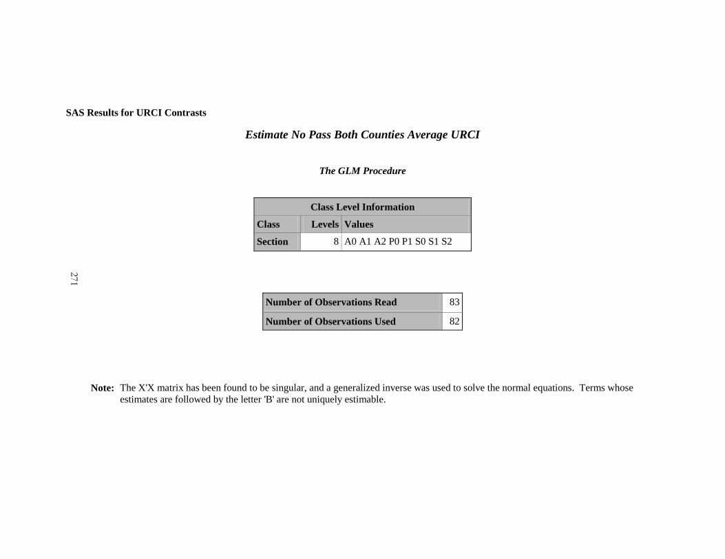
271

SAS Results for URCI Contrasts

Estimate No Pass Both Counties Average URCI

The GLM Procedure

Class Level Information

Class Levels Values

Section 8 A0 A1 A2 P0 P1 S0 S1 S2

Number of Observations Read 83

Number of Observations Used 82

Note: The X'X matrix has been found to be singular, and a generalized inverse was used to solve the normal equations. Terms whose estimates are followed by the letter 'B' are not uniquely estimable.

272

The GLM Procedure

Dependent Variable: URCI

Source DF Sum of

Squares Mean Square F Value Pr > F

Model 11 3286.317073 298.756098 16.90 <.0001

Error 70 1237.207317 17.674390

Corrected Total 81 4523.524390

R-Square Coeff Var Root MSE URCI Mean

0.726495 4.626702 4.204092 90.86585

Source DF Type I SS Mean Square F Value Pr > F

Section 7 2452.088027 350.298290 19.82 <.0001

Dust 1 128.604882 128.604882 7.28 0.0087

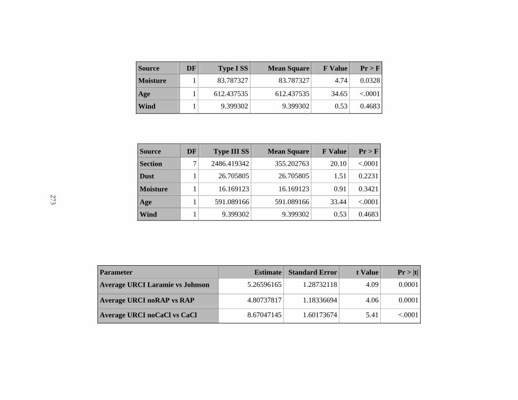
273

Source DF Type I SS Mean Square F Value Pr > F

Moisture 1 83.787327 83.787327 4.74 0.0328

Age 1 612.437535 612.437535 34.65 <.0001

Wind 1 9.399302 9.399302 0.53 0.4683

Source DF Type III SS Mean Square F Value Pr > F

Section 7 2486.419342 355.202763 20.10 <.0001

Dust 1 26.705805 26.705805 1.51 0.2231

Moisture 1 16.169123 16.169123 0.91 0.3421

Age 1 591.089166 591.089166 33.44 <.0001

Wind 1 9.399302 9.399302 0.53 0.4683

Parameter Estimate Standard Error t Value Pr > |t|

Average URCI Laramie vs Johnson 5.26596165 1.28732118 4.09 0.0001

Average URCI noRAP vs RAP 4.80737817 1.18336694 4.06 0.0001

Average URCI noCaCl vs CaCl 8.67047145 1.60173674 5.41 <.0001

274

Parameter Estimate Standard Error t Value Pr > |t|

Intercept 102.0479995 B 2.22689771 45.83 <.0001

Section A0 4.6065644 B 2.11742462 2.18 0.0330

Section A1 -2.1220789 B 1.88501433 -1.13 0.2641

Section A2 -11.3945134 B 1.92136966 -5.93 <.0001

Section P0 6.3220059 B 2.21834442 2.85 0.0057

Section P1 -3.1984453 B 1.88878748 -1.69 0.0948

Section S0 -11.3108234 B 2.26424636 -5.00 <.0001

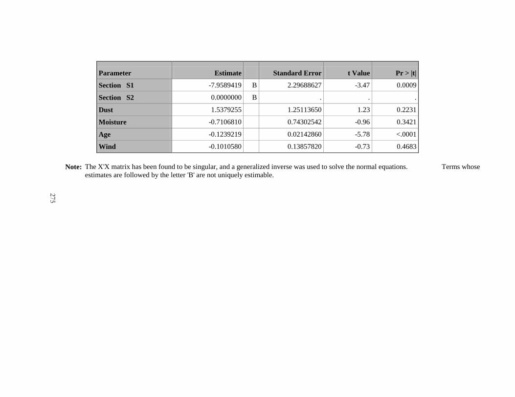
275

Parameter Estimate Standard Error t Value Pr > |t|

Section S1 -7.9589419 B 2.29688627 -3.47 0.0009

Section S2 0.0000000 B . . .

Dust 1.5379255 1.25113650 1.23 0.2231

Moisture -0.7106810 0.74302542 -0.96 0.3421

Age -0.1239219 0.02142860 -5.78 <.0001

Wind -0.1010580 0.13857820 -0.73 0.4683

Note: The X'X matrix has been found to be singular, and a generalized inverse was used to solve the normal equations. Terms whose estimates are followed by the letter 'B' are not uniquely estimable.