TASK QUARTERLY 5 No 4 (2001), 579–594 PERFORMANCE PREDICTION OF CENTRIFUGAL PUMPS WITH CFD-TOOLS ERIK DICK, JAN VIERENDEELS, SVEN SERBRUYNS AND JOHN VANDE VOORDE Department of Flow, Heat and Combustion Mechanics, Ghent University, Sint-Pietersnieuwstraat 41, 9000 Gent, Belgium [email protected](Received 19 July 2001) Abstract: The CFD-code FLUENT, version 5.4, has been used for the flow analysis of two test pumps of end-suction volute type: one of low specific speed and one of medium specific speed. For both, head as function of flow rate for constant rotational speed is known from experiments. FLUENT provides three calculation methods for analysis of turbomachinery flows: the Multiple Reference Frame method (MRF), the Mixing Plane method (MP) and the Sliding Mesh method (SM). In all three methods, the flow in the rotor is calculated in a rotating reference frame, while the flow in the stator is calculated in an absolute reference frame. In the MRF and MP methods steady flow equations are solved, while in the SM method, unsteady flow equations are solved. The SM method does not introduce physical approximations. The steady methods approximate the unsteady interaction between rotor and stator. The cost of the unsteady method is, however, typically 30 to 50 times higher than the cost of the steady methods. It is found that the MRF and MP methods lead to completely erroneous flow field predictions for flows far away from the best efficiency point. This makes the steady methods useless for general performance prediction. Keywords: centrifugal pumps, CFD-analysis, performance prediction 1. Introduction The CFD-code FLUENT provides three calculation methods for the analysis of tur- bomachinery flows: the Multiple Reference Frame method, the Mixing Plane method and the Sliding Mesh method. The first two methods are basically steady flow methods. In the Multiple Reference Frame method, the rotor is kept at a fixed position. The governing equations are solved for the rotor in a rotating reference frame, so including Coriolis and centrifugal forces. The governing equations for the stator are solved in an absolute reference frame. As coupling between both parts, continuity of velocity components and pressure is imposed. In principle, unsteady equations can be solved but as the main source of unstead- iness, i.e. the movement of the impeller is neglected, the unsteady solution has not much meaning. The flow field is dependent on the relative position of the impeller and the volute. For a complete analysis, the flow for different relative positions has to be calculated. The technique is also known under the name Frozen Rotor method. In the Mixing Plane method, tq0405e7/579 26 I 2002 BOP s.c., http://www.bop.com.pl
Transcript
TASK QUARTERLY 5 No 4 (2001), 579–594
PERFORMANCE PREDICTION OF CENTRIFUGALPUMPS WITH CFD-TOOLS
ERIK DICK, JAN VIERENDEELS, SVEN SERBRUYNSAND JOHN VANDE VOORDE
Department of Flow, Heat and Combustion Mechanics,Ghent University,
Abstract: The CFD-code FLUENT, version 5.4, has been used for the flow analysis of two test pumps ofend-suction volute type: one of low specific speed and one of medium specific speed. For both, headas function of flow rate for constant rotational speed is known from experiments. FLUENT provides threecalculation methods for analysis of turbomachinery flows: the Multiple Reference Frame method (MRF),the Mixing Plane method (MP) and the Sliding Mesh method (SM). In all three methods, the flow in therotor is calculated in a rotating reference frame, while the flow in the stator is calculated in an absolutereference frame. In the MRF and MP methods steady flow equations are solved, while in the SM method,unsteady flow equations are solved. The SM method does not introduce physical approximations. The steadymethods approximate the unsteady interaction between rotor and stator. The cost of the unsteady method is,however, typically 30 to 50 times higher than the cost of the steady methods. It is found that the MRF andMP methods lead to completely erroneous flow field predictions for flows far away from the best efficiencypoint. This makes the steady methods useless for general performance prediction.
1. IntroductionThe CFD-code FLUENT provides three calculation methods for the analysis of tur-
bomachinery flows: the Multiple Reference Frame method, the Mixing Plane method andthe Sliding Mesh method. The first two methods are basically steady flow methods. Inthe Multiple Reference Frame method, the rotor is kept at a fixed position. The governingequations are solved for the rotor in a rotating reference frame, so including Coriolis andcentrifugal forces. The governing equations for the stator are solved in an absolute referenceframe. As coupling between both parts, continuity of velocity components and pressure isimposed. In principle, unsteady equations can be solved but as the main source of unstead-iness, i.e. the movement of the impeller is neglected, the unsteady solution has not muchmeaning. The flow field is dependent on the relative position of the impeller and the volute.For a complete analysis, the flow for different relative positions has to be calculated. Thetechnique is also known under the name Frozen Rotor method. In the Mixing Plane method,
580 E. Dick, J. Vierendeels, S. Serbruyns and J. Vande Voorde
as in the previous method, relative and absolute reference frames are used, but exchangingcircumferentially averaged flow quantities does the coupling between both. In principle,the result is independent of the relative position of impeller and volute. The Sliding Meshmethod is a truly unsteady method. Also a rotating and an absolute reference frame areused but the effect of displacement due to rotation is taken into account. At each time step,the rotor is set at its correct position and fluxes are interpolated on the common slidingsurface between both parts. Apart from some diffusion due to the interpolation, there is nomajor approximation in the representation of the unsteadiness. So, for the calculation of thehydraulic performance, the Sliding Mesh method can be seen as a reference method.
The computational effort for the sliding mesh technique is typically a factor 50 largerthan the effort for a mixing plane technique and a factor 30 larger than the effort for a frozenrotor technique. So for practical applications, it is necessary to know how far the steadytechniques are realistic.
The use of CFD-tools to analyse the flow field in turbomachines and to predictperformance parameters has gained enormous popularity in recent years. This processhas been stimulated by the availability of commercial packages allowing turbomachineryanalysis. Although it is very well known that the flow field in a turbomachine is inherentlyunsteady, most calculations nowadays are done with steady methods. All this has to do withthe cost of unsteady calculations. The simplest steady calculation method is, as alreadymentioned, the mixing plane method. It has the particular advantage that the calculationof the rotor flow and the stator flow can be done almost independent of each other. Forapplications to end-suction volute centrifugal pumps, only one blade channel of the impellerhas to be calculated. The circumferentially averaged flow quantities at the outlet of theimpeller form then the inlet variables for the calculation of the volute. The technique iswidely used in axial flow machines. Examples of calculations of this type in low specificspeed and medium specific speed mixed flow pumps with axial diffusers are given byTakamara and Goto [1] and Goto [2]. Sedlar and Mensik [3] give examples of calculationsof radial flow pump stages with semi-axial and radial diffusers. In the cited references,it is reported that the mixing plane method leads to accurate performance predictions. Thisis not completely surprising since the method is known to perform well for axial flowmachines. In the cited examples there is no volute and as a consequence, the flow characteris rather similar to the flow character in axial flow machines. Sedlar and Mensik alsoperformed calculations with the frozen rotor technique. They also report good results withthis technique. In volute pumps, the circumferential variation of pressure imposed by thevolute on the impeller for flows different from design flow can be quite large, especiallyfor low flow rates. It is also well known that the inhomogeneous pressure distributionimposed on the impeller exit is felt inside the impeller, as shown by Sideris and Van denBraembussche [4], Miner et al. [5] and Liu et al. [6]. In principle, the frozen rotor techniqueallows one to take into account the influence of the pressure variation on the impeller flow.Therefore it is tempting to use this technique for the flow analysis of volute centrifugalpumps, although the unsteadiness caused by the rotor/stator interaction is neglected. Goodresults have been obtained with the frozen rotor technique by Cugal and Bache [7] fora volute centrifugal pump and by Gugau et al. [8] for a volute low-speed centrifugalcompressor. The results obtained in the first reference might be not completely representativesince the pump has a double tongue volute. This causes that the circumferential pressure
Performance Prediction of Centrifugal Pumps with CFD-tools 581
distortion for low flow rates is less pronounced than for a single tongue volute. The authorsof the second reference observe non-real flow patterns for low flow rates. As a consequence,they recommend the use of the mixing plane method. They found that the quality of theprediction of the pressure ratio as function of the mass flow is equally good for both steadymethods. The discrepancy between calculated and measured values for the pressure ratiowas only about 1–2%. This is a surprisingly good result.
In the present study, flow analysis is done on two test pumps of end-suction volutetype, well known from the literature. The first pump is a plexiglas research pump from theUniversity of Virginia [5]. It has low specific speed and a two-dimensional form. The secondpump is a medium specific speed pump from the British Hydraulic Research Association [9].The pump has doubly curved vanes. For both pumps, the performance characteristics areknown from experiments. We analyse here how far the CFD-methods typically available ina commercial package can be used for the prediction of the head as function of flow ratefor constant rotational speed. We take the frozen rotor technique as the central technique ofthe investigation. In particular, we want to determine how far this technique can take intoaccount the influence of the circumferential pressure variation, caused by the volute for flowsdifferent from best efficiency flow, on the impeller flow. The sliding mesh method is used asa reference technique. It is only used for three flow rates on pump 1. These calculations aremeant to demonstrate that this technique is able to reproduce the performance parameterscorrectly. The mixing plane method is used for one flow much different from best efficiencyflow in order to verify the quality of the predictions of this method.
2. MethodologyA hybrid mesh is created using FLUENT’s preprocessor GAMBIT. The geometry is gen-
erated with the aim of subdivision into multiple blocks. First, the impeller is generated.One impeller channel is meshed and is then rotationally copied the necessary number oftimes. For the first pump, the impeller is completely two-dimensional. The impeller meshis made with hexahedra and wedge cells. For the second pump, the impeller channel ismuch more complex. The mesh is made in a completely unstructured way, mainly usingtetrahedra, but other cell forms like pyramids, hexahedra and wedges also occur. The inletchannel is meshed for both pumps with prisms. The volute in both pumps is too complex fora structured grid. The meshing is done in an unstructured way, mainly using tetrahedra. Forthe first pump, the cross section is rectangular. The precise cross section shape of the volutefor the second pump cannot be obtained from [9]. It was approximated by a trapezoid. Forthe first pump, the outlet channel has a constant rectangular section. This channel is meshedin a structured way using hexahedra. In the second pump, a diffuser that changes sectionfrom trapezoid to circle follows the volute. This diffuser is meshed in an unstructured way,mainly using tetrahedra. A constant section circular tube meshed with prisms follows thediffuser. Figure 1 shows the complete mesh for pump 1 and the mesh for pump 2 up to theoutlet of the volute. In pump 1, the interface between the impeller and the volute is splitinto two surfaces for the sliding mesh calculation. Since these surfaces are represented ina piecewise manner, a small gap is necessary between them in order to allow the rotationof the impeller. Data were interpolated between these surfaces, neglecting the gap. Forpump 2, no sliding mesh calculations have been done. A particular aspect of the mesh forthis pump is that the mesh is split into two parts at the interface between the volute outlet
582 E. Dick, J. Vierendeels, S. Serbruyns and J. Vande Voorde
and diffuser inlet. The interface plane is treated as a mixing plane, as explained later. Forthe frozen rotor calculations, two positions of the impeller have been used. In position 1,the mid of an impeller channel corresponds to the tongue of the volute. In position 2, animpeller blade corresponds to the tongue. The impeller of pump 1 is of closed type. In thecalculations, the axial gap between the impeller and the pump house has been set to zero.So, leakage flow is neglected. The impeller of pump 2 is of open type and there is a smallgap in axial direction between the impeller blades and the shroud. The gap has been set toa small value so that exactly one cell is obtained in the gap. The gap at the backside of theimpeller has been set to zero. This has as a consequence that in the calculations the leakageflow is not correctly calculated. The total number of cells for pump 1 is about 300 000. Forpump 2, it is about 550 000.
Table 1 summarises the main geometrical parameters of the two pumps. Full detailson the geometry can be found in [5, 9]. Both pumps have an annular space following theimpeller with a larger width than the outlet width of the impeller. The annular space definesthe volute tongue gap.
Table 1. Geometric properties of the test pumps
Pump 1 Pump 2
Diameter inlet tube 38.3 mm 138 mmInlet diameter impeller 50.8 mm 67.8 mm (hub), 102.8 (mean),
139.9 mm (shroud)Inlet angle impeller 16° 30° (hub), 19.5° (mean),
14° (hub)Inlet width impeller 24.6 mm 49.2 mmOutlet diameter impeller 203.2 mm 203.2 mmOutlet angle impeller 16° 23°Outlet width impeller 24.6 mm 31.75 mmNumber of blades 4 5Thickness of the blades 3 mm 5.5 mmOutlet diameter annular space 215.9 mm 223.6 mmWidth of the annular space 25.8 mm 44.5 mmWidth volute 25.8 mm (constant) 44.5 mm (base width)Outlet section volute 2785 mm2 3890 mm2
Outlet section diffuser constant section 8171 mm2
Rotational speed used in test 620 rpm 2910 rpmCorresponding nominal flow rate 6.3 l/s 60 l/s
The equations solved are the three-dimensional Reynolds-averaged Navier-Stokesequations. The fluid is incompressible. The segregated solver with implicit formulationis used. For the convective terms second order upwinding is used. For the pressurecorrection, the SIMPLE scheme is used.
As a turbulence model, the realizable k-" model is used with non-equilibrium wallfunctions. The mass flow rate and the flow direction normal to the boundary are imposedat the inlet. The turbulence intensity is determined from the formula for a fully developedpipe flow. A uniform turbulence length scale is imposed calculated from the diameter ofthe inlet pipe. At the outlet, flow parameters are extrapolated from the interior.
Calculations are typically started from a no-flow initial condition, with the impeller atstandstill. The rotational speed is increased gradually until the final speed is reached. Thefirst flow rate calculated has always been the nominal flow rate. Often the calculations for
584 E. Dick, J. Vierendeels, S. Serbruyns and J. Vande Voorde
some flow rate can be started from the result of a neighbouring flow rate, without goingthrough the procedure of gradual increase of the rotational speed. For the very low flowrates this is not possible since the general flow pattern changes significantly when loweringthe flow rate. Calculations for low flow rates have to be started from no-flow conditions.
3. Results of frozen rotor calculations
Figure 2 shows the calculated head as function of flow rate for pump 1, obtained bythe frozen rotor technique for the two positions of the impeller, in comparison with theexperimental data. For a flow rate 7 l/s, i.e. somewhat above the nominal flow rate (6.3 l/s),the predictions are quite good. The quality of the predictions deteriorates for flow ratesdifferent from the nominal flow rate. In particular for low flow rates, the calculations givea serious underprediction of the head. Figure 3 shows the corresponding result for pump 2.The same observations are made here. The calculations for pump 2 have been done in twoparts. As already said, a mixing plane is introduced at the outlet of the volute. This turnedout to be necessary for the calculation of the diffuser. Since in the frozen rotor technique,the rotor stands still, wakes shed from the blades of the impeller stay localised in space.For either of the two positions of the impeller, a wake causes an unphysical flow separationon the upper or lower wall of the diffuser. In reality, this does not happen since wakes arelargely mixed in the volute and are unsteady. No localised separation occurs in the diffuser.To mimic this physical mixing process, a mixing plane was introduced at the end of thevolute. The consequence is that the calculation of the diffuser and the outlet pipe becomesindependent of the calculation of the rest of the pump.
Figure 2. Pump 1: head as function of flow rate. Frozen Rotor predictions
Figure 4 shows the distribution of static pressure in an orthogonal plane at the midof the impeller and the volute for pump 1, in position 1, for the nominal flow rate (6.3 l/s).The distribution of the pressure is very similar for all channels in the impeller. The pressuregradient due to the centrifugal force can be seen in the volute. There is basically no pressuregradient in the circumferential direction in the volute. Figure 4 shows also the distributionof the static pressure for flow rate 7.5 l/s (120% of the nominal flow rate). The distributionof the pressure in the impeller channels is still very similar for all channels. There is nowa slight decrease of the pressure in the circumferential direction in the volute, in the senseof the flow.
586 E. Dick, J. Vierendeels, S. Serbruyns and J. Vande Voorde
Figure 5. Distribution of static pressure (top) and absolute velocity (bottom)in the mid plane for pump 1. Low flow rate (2.54 l/s)
Figure 5 shows the distribution of the static pressure and absolute velocity for flowrate 2.54 l/s (40% of nominal flow rate) in the mid plane of the impeller for position 2.Only the pressure distribution in the impeller is shown in order to better illustrate thedifference between the different impeller channels. The increase in pressure in the volute incircumferential direction in the sense of the flow is felt at the exit of the impeller channel,causing the unequal pressure distributions in the channels. At first sight, one would considerthat this behavior corresponds to reality. Figure 6 shows a vector plot of the relative andabsolute velocity in the mid plane of the impeller, projected into this plane, corresponding tothe pressure plot of Figure 5. In the vector plot of relative velocity, large recirculation zonescan be seen in the impeller channels exposed to the largest volute pressure. Flow velocitiesare very low in these channels. The flow vectors at the periphery of the impeller pointinwards, so in the mean there is reversed flow in these channels. The impeller channels
Performance Prediction of Centrifugal Pumps with CFD-tools 587
Figure 6. Vector plot of relative velocity (top) and absolute velocity (bottom)for low flow rate for pump 1
exposed to the lowest volute pressure have a flow that is well aligned with the impellerblades. The inflow at the periphery in the impeller channel exposed to the largest counterpressure can clearly be seen in a vector plot of the absolute velocity. At this stage, one canalready doubt about the physical correctness of the obtained flow pattern by verifying thework exchange in the impeller. On the basis of an integral of the moment of momentumflux through a cylindrical surface around the impeller, it could be verified that the workexchanged by the impeller and the flow is lower than the energy increase in the fluid.This has as consequence that the calculated hydraulic efficiency of the pump is largerthan one.
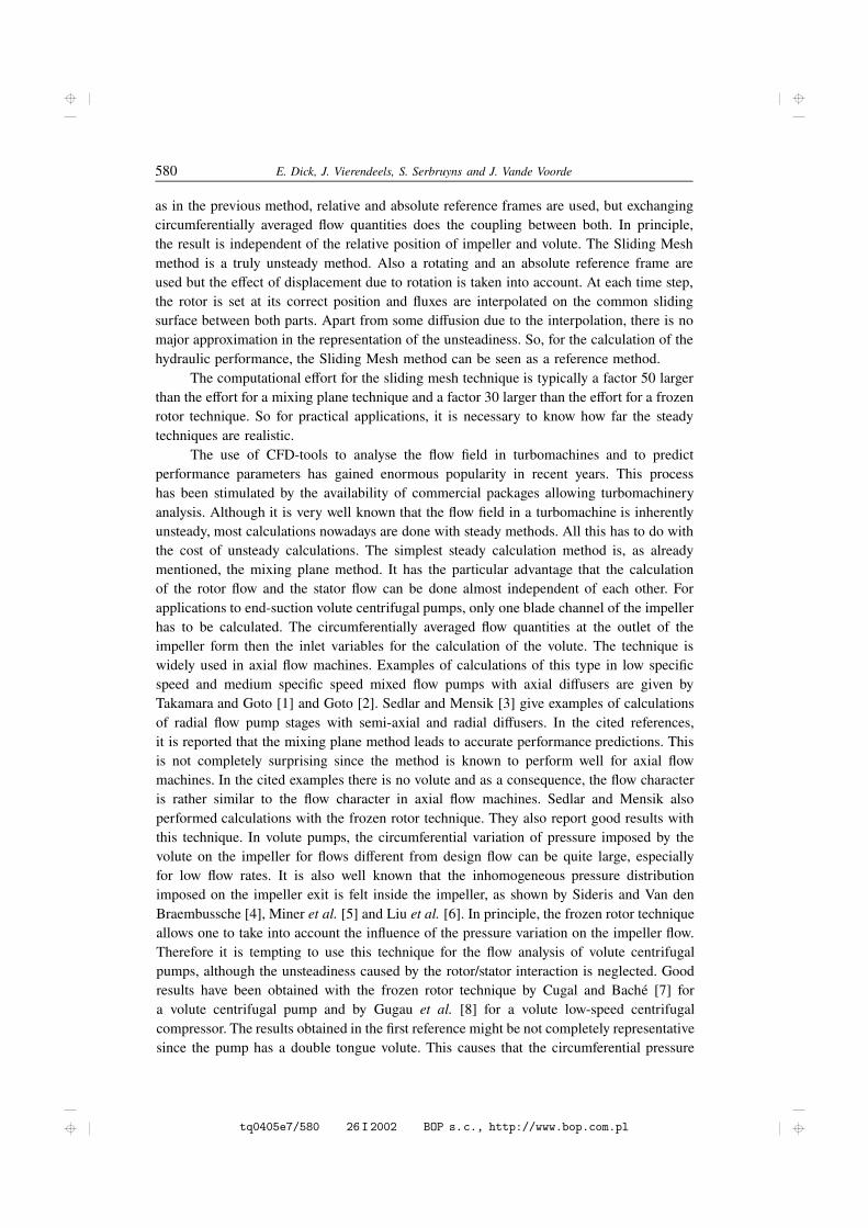
Figures 7 and 8 show the distribution of the static pressure on a mean stream surfacein pump 2, projected on an orthogonal plane for nominal flow rate (60 l/s), high flowrate (90 l/s) and low flow rate (30 l/s). The same observations apply as for pump 1, i.e.the pressure distribution in the impeller adjusts to the pressure distribution in the volute.As such, this is as expected since precise continuity of pressure is imposed as interface
588 E. Dick, J. Vierendeels, S. Serbruyns and J. Vande Voorde
Figure 7. Distribution of static pressure in the mean stream surface of pump 2:nominal flow rate (60 l/s)
condition between the impeller and the volute. Again the observation is that for low flowrate the velocity distribution (not shown) is not likely to be physically correct.
4. Comparison between frozen rotor and sliding mesh results
For three flow rates of pump 1, sliding mesh calculations have been performed. InFigure 9, the calculated head is shown in comparison to the experimental result and tothe results of the frozen rotor calculation. The sliding mesh calculations lead to someoverprediction of the head. The overprediction increases with decreasing flow rate. A slightoverprediction of the head is certainly a good feature. We have to remember that the leakageflow of the pump cannot be obtained by the present calculations, since the gap between theimpeller and the shroud is set to zero. Taking into account a correction for leakage losseswould certainly bring the calculated results for the sliding mesh technique very close to theexperimental data.
Figure 10 shows the vector plot of absolute velocity in the mid plane of the pump,projected into this plane for flow rate 2.54 l/s. This figure should be compared to Figure 6.Obviously, there is no reversed flow detected by the sliding mesh calculation.
Figure 11 compares the radial velocity components for the frozen rotor and slidingmesh calculations for flow rate 2.54 l/s. From this comparison, the conclusion is thatthe prediction of reversed flow by the frozen rotor method is completely erroneous. Thesliding mesh calculation shows that the distribution of the flow over the impeller is almosthomogeneous. The observation is that the impeller flow almost does not react to thepressure variation in the volute. Figure 12 shows the comparison for pressure. The pressuredistributions obtained from both calculations are not identical but the general behavior isthe same. The sliding mesh calculation shows that the pressure distribution in the impeller
Performance Prediction of Centrifugal Pumps with CFD-tools 589
Figure 8. Distribution of static pressure in the mean stream surface of pump 2.Top: high flow rate (90 l/s). Bottom: low flow rate (30 l/s)
adjusts to the pressure distribution in the volute. This does, however, not lead, as is shownby Figure 10, to a velocity distribution that follows the pressure distribution.
The explanation of this phenomenon is to be found in the inertia of the fluid. Fora flow rate of 2.54 l/s for pump 1, it can be verified that the time needed for a fluidparticle to flow through the impeller is approximately equal to the time needed for onerotation of the impeller. This means that the flow through an impeller channel is in realityexposed to a complete cycle of pressure variation in the volute and, as a consequence,
590 E. Dick, J. Vierendeels, S. Serbruyns and J. Vande Voorde
Figure 9. Head as function of flow rate for pump 1: comparison of Frozen Rotorand Sliding Mesh calculations
Figure 10. Vector plot of absolute velocity in the mid plane of pump 1 for flow rate 2.54 l/s,obtained by the Sliding Mesh method
reacts approximately in the same way as if it were exposed to the mean pressure in thevolute. By this interpretation, it can now be understood why the frozen rotor calculation isfundamentally incorrect.
5. Mixing plane calculationThe conclusion formulated in the previous section leads to the expectation that
mixing plane calculations might perform quite well as a performance prediction method.Figure 13 shows the distribution of radial velocity and static pressure obtained by themixing plane method for flow rate 2.54 l/s for pump 1. Reversed flow is observed. So,the flow field prediction is, like for the frozen rotor calculation, not realistic. Remark thatthere is circumferential variation of flow properties in the impeller. The reason is that forreversed flow, the static pressure in the volute becomes the inflow condition for the impeller.Calculations have also been done with an isolated rotor and a constant counter pressure.Backflow was also obtained.
592 E. Dick, J. Vierendeels, S. Serbruyns and J. Vande Voorde
Figure 12. Distribution of static pressure for Sliding Mesh (top) and Frozen Rotor (bottom) calculations,pump 1, 2.54 l/s
6. ConclusionSteady calculation methods like the Frozen Rotor method and the Mixing Plane
method cannot be used with confidence to analyse the performance of volute centrifugalpumps. This is in contrast to applications to turbomachines with circumferentially periodicflow character. The basic reason for the erroneous behaviour of the steady methods is theinability to represent the effect of the fluid leaving the impeller. This inertia effect causes thatthe pressure variation imposed by the volute for flows much different from best efficiencyflow is seen in a largely filtered way by the fluid in the impeller. The real flow is much more
Performance Prediction of Centrifugal Pumps with CFD-tools 593
Figure 13. Distribution of radial velocity (top) and static pressure (bottom)for Mixing Plane calculations, pump 1, 2.54 l/s
homogeneous than predicted with the Frozen Rotor and the Mixing Plane methods. Onlya truly unsteady method like the Sliding Mesh technique is able to correctly reproduce thisflow behaviour. The predicted performance by the Sliding Mesh method can be used withconfidence.
References[1] Takemura T and Goto A 1996 Journal of Turbomachinery 118 552[2] Goto A 1997 Prediction of diffuser pump performance using 3D viscous stage calculation FEDSM97-
594 E. Dick, J. Vierendeels, S. Serbruyns and J. Vande Voorde
[3] Sedlar M and Mensik P 1999 Investigation of rotor/stator interaction influence on flow fields in radialflow pumps Proc. 3rd European Conference on Turbomachinery, IMechE, pp. 1017–1025
[4] Sideris M and Van den Braembussche R 1987 Journal of Turbomachinery 109 48[5] Miner S, Beaudoin R and Flack R 1989 Journal of Turbomachinery 111 205[6] Liu C, Vafidis C and Whitelaw J 1994 Journal of Fluids Engineering 116 303[7] Cugal M and Bache G 1997 Performance prediction from shutoff to runout flows for a complete stage
of a boiler feed pump using computational fluid dynamics FEDSM97-3334 ASME Fluids EngineeringDivision Summer Meeting
[8] Gugau M, Matyschok B and Stoffel B 2001 Experimental and 3D numerical analysis of the flowfield in a turbocharger compressor Proceedings: Fourth European Turbomachinery Conference SGE,pp. 297–306
[9] Anonymous 1982 Design specifications. IMechE Conference Publications C184/82;and Anderson H, Salisbury A, Dziewulski T and Burgoyne D 1982 Discussion. IMechE ConferencePublications C186/82