Permanent Excess Demand as Business Strategy: An analysis of the Brazilian higher-education market Insper Working Paper WPE: 317/2013 Eduardo Andrade Rodrigo Moita Carlos Silva Inspirar para Transformar
Transcript
Permanent Excess Demand as Business Strategy: An analysis of the Brazilian higher-education market
c Department of Economics, Pontifícia Universidade Católica do Rio Grande do Sul (PUC-RS), Address: Av Ipiranga,
6681, prédio 50, sala 1001 Porto Alegre – RS, Brazil. Email: [email protected] (corresponding author).
2
Abstract
Many Higher Education Institutions (HEIs) establish tuition below the equilibrium price to generate permanent excess demand. This paper first builds on Becker’s (1991) theory to understand why the HEIs price in this way. The fact that students are both consumers and inputs on the education production function gives rise to an equilibrium where some firms have permanent excess demand. Second, the paper analyzes this equilibrium empirically. The results show that the HEIs give up 7.6% of the revenue coming from a freshman class in order to have better students and to differentiate themselves as high quality in the market.
I. Introduction
Microeconomics manuals teach that in equilibrium, the amount demanded for a good or
service must equal the amount offered. In the higher-education market, this principle does not hold.
Instead, many higher-education institutions (HEIs) limit the number of available spaces to
guarantee excess demand every year. The same phenomenon can be observed in other markets,
especially service markets, but the rationale behind excess demand in higher education is not the
same as the one that applies to restaurants or large events. In these latter cases, excess demand aims
at keeping these places busy, never empty, since it brings value to these services. In education, the
student, in addition to being a consumer, is also a factor of production—the quality of the output is
a function of the quality of the student body. For this reason, given the characteristics of the HEI,
the institution sets tuition below equilibrium price to increase the quality of its students through
excess demand and greater selectivity.
A characteristic of the Brazilian higher education market is that there is strong market
differentiation within HEIs. There are HEIs with good reputation, which charge high tuitions and
have hotly disputed selection processes, and others that are little known outside their local area and,
although they charge low tuitions, have empty slots. Among private Business Administration
3
schools in São Paulo in 2006, for example, the fees range from 170 to 2250 Reais (or from US$ 106
to US$ 14152), and the ratio of candidates to slots ranges from 0.17 to 11.5.
This paper analyzes the HEI market and attempts to answer three interrelated questions: (a)
how do we theoretically understand the existence of the HEI that opts for the strategy of
maintaining permanent excess demand? (b) is this strategy justifiable? (c) how much revenue does
the HEI give up to increase the selectivity of its admissions process and, consequently, the quality
of its students?
We build on the ideas of Becker (1991) to explain why some HEIs maintain permanent
excess demand while others do not. Next, using a database of business schools in the state of São
Paulo, we estimate the demand for higher education. The empirical results show that the quality of
the student body, the tuition, and the quality of the professors are relevant in determining the
demand of the market. The relevance of the quality of the student body justifies the strategy of an
HEI that opts for excess demand and confirms the theory that will be developed in the next section:
demand for the school hinges on the quality of the students and, ultimately, responds positively to
the selectivity imposed by the HEI. Finally, using the econometric results we present the total
“investment” in selectivity made by São Paulo HEIs in their business programs. This total, which
surpasses five million Reais (or US$ 3.14 million – 7.6% of the revenue) per year, can be
understood as an investment in differentiation.
In a more general setting, this paper analyzes the influence of a positive externality in
consumer’s choice on market equilibrium.3 The fact that consumer’s choice defines the quality of
the good being sold, endogenously lead to market vertical differentiation, in the sense that quality is
not a firm’s control variable. This externality affects the organization of the industry in many
2 The exchange rate used in this paper is R$ 1.59 reais to buy one dollar, of June 14th, 2011.
3 Glaeser and Scheinkman (2001) call this positive externality ‘non-market interactions’, while Becker and Murphy
(2000) call it ‘social interactions’. Glaeser and Scheinkman (2001) provides a survey of the theoretical literature on this
subject. Despite its relevance on market equilibrium, there is little connection between this area and teh field of
industrial organization, with Becker (1992) being a notable exception.
4
dimensions: pricing, product differentiation, market structure and competition.4 The focus of this
paper is on pricing and market differentiation.
While Becker (1991) theoretically shows why some restaurants having long queues for
tables do not raise prices, this paper estimates the “investment on queues”. The higher education
market is specially appropriated for this study because there are data about all the candidates,
including those students that failed in the selecting process. In a restaurant-market context, it would
be as if we knew the numbers of clients and the number of people who give up eating at a given
restaurant because of its long queues.
The selection of better students in higher education is well documented by the literature, but
how to measure its impact on the education output is a controversial question (see Winston and
Zimmerman, 2003). Instead of measuring this effect, the focus of this work is to better understand
how the existence of those effects modifies the market equilibrium. Thus, we estimate (a) on one
side, how the selectivity of HEIs (considering the quality of incoming students as a proxy) affects
the demand curve, and (b) on the other side, how much the HEIs invest in selectivity to maximize
their long term profits by maintaining permanent excess demand.
There is a series of studies that examine the importance of tuition on the decision to pursue
higher education. Ehrenberg (2004) makes a review of the literature, corroborating the notion that a
higher tuition and fewer financial incentives, such as scholarships, reduce the motivation to study at
an HEI. Other characteristics that may affect student preferences are less studied.
Four papers follow this line of research and are closely related to our study. Gallego and
Hernando (2008) also use a discrete choice model in Chilean high schools to estimate the effects of
the voucher system on student well-being and socio-economic segregation. Monks and Ehrenberg
(1999) use panel data to evaluate the impact on the demand for universities of the U.S. News and
World Report rankings, the most traditional ranking in the U.S market. They conclude that a lower
position in the ranking is detrimental to the university: fewer accepted students decide to enroll; the
4 See Shaked and Sutton (1983) for an analisis of competition in vertically differentiated markets.
5
quality of new classes decreases, as measured by the admissions test; and the net tuition paid by the
student is lower because the university has to be more generous in granting financial aid to attract
students from the smaller group of applicants.
Long (2004) examines how different cohorts of students in the United States choose which
HEI to attend based on their own characteristics and those of the HEI, such as tuition, quality of
student body, percentage of professors with doctorates and student/teacher ratio. Long’s study
concludes that the quality of the faculty is the most important factor in the student’s decision, a
result we also find here.
Kelchtermans and Verboven (2009) study student choice in the Belgium region of Flandres.
They use a nested logit model that analyzes the problem of whether and where to pursue higher
education. They conclude that courses are close substitutes, and that a tuition increase would not
affect the decision of whether to study but affect the decision of where to study.
Despite the fact that all these papers also estimate a demand for educational institutions, the
details of the method we employ and our goals are quite distinct from the others. We chose to
restrict our analysis to business administration courses only. Implicitly, we assume that business
administration is not a substitute with other courses, such as biology or engineering.
The rest of this article is organized as follows. In the next section, we discuss why a HEI
could use the strategy to operate with excess demand. Section 3 explains the methodology and data
employed. The results are presented in Section 4. The final section concludes the analysis.
II. Theoretical Discussion
The fundamental hypothesis of Becker (1991), who studies the causes of excess demand in
the restaurant industry, is that the individual’s demand depends on the other individuals’ demand.
The author suggests that eating out, attending a cultural event or discussing a book are social
6
activities in which people consume the product or service together, and therefore, the number of
people sharing the same product influences the utility of the individual consumer.
In the case of higher education, this argument acquires an additional facet: in addition to
student interaction, whose positive effect on learning is a function of the qualification and
performance of the cohort (the peer effect, which does not occur in the case of restaurants), the
quality and success of the graduates serve as signals to the market of the quality of the HEI.
Therefore, good students tend to generate good graduates, who contribute to the reputation of the
institution. In contrast with restaurants, the quality of enrolled students is fundamental to the choice
of the potential student. Because greater selectivity increases the quality of the incoming class, we
may conclude that excess demand creates demand. Therefore, excess demand is the result of the
maximization of long-term profit.
The coexistence of HEIs with different strategies—with or without excess demand—can be
understood using Becker’s model (1991). Becker (1991) does not distinguish between the short and
long term, but his analysis corresponds to what we consider to be long term here.
This differentiation seems important with respect to higher education because we assume
that permanent excess demand builds the HEI’s reputation, which in turn determines its short-term
demand curve. If an HEI with a good reputation raises its tuition to eliminate excess demand, the
demand during the year in question (the short term) will not be altered. In the short term, tuition set
below equilibrium generates excess demand (and greater selectivity), which, in the long term, will
shift the short-term demand curve to the right. It happens because, in this analysis, each short-term
curve is determined (and sustained) by a given level of excess demand.
For the HEI that maintains excess demand, this movement is sufficiently large for a given
interval of prices, and consequently, the long-term demand will be positively inclined in this
interval (Fig. 1). When the price reaches a sufficiently high level, the large shifts in demand stop,
and the long term demand becomes negatively sloped. In this case, the tuition rate that maximizes
profit (P3) will be below the short term equilibrium price (P4).
7
Fig. 1: Long-term equilibrium with excess demand
S
D1
D2
D3
a b
P1
P2
P3
P4
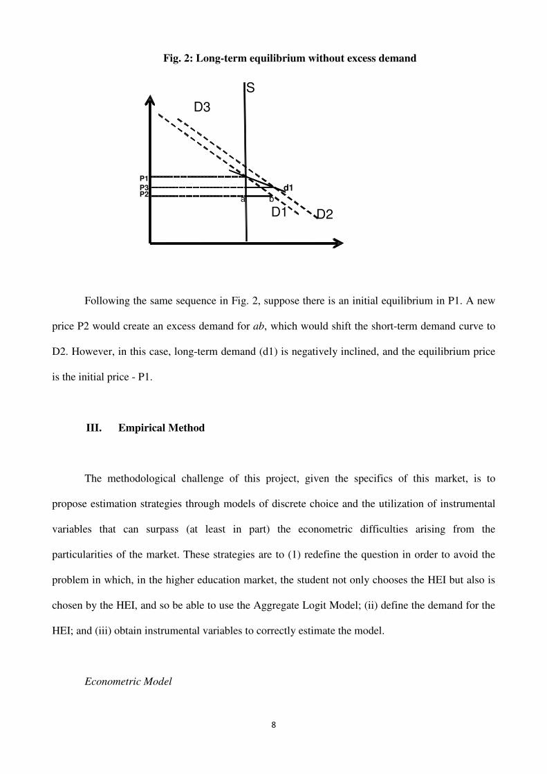
Yet, in the case of the HEIs that do not maintain excess demand, the long-term demand
curve will be negatively sloped because excess demand does not create a sufficiently large shift in
the short term (Fig. 2).
In analyzing Fig. 1, an initial equilibrium in P1 is determined by the D1 demand and supply
S. Next, an HEI reduces its price to P2 and creates an excess demand of ab. In the long term, for
this excess demand, the short-term curve turns out to be D2, which allows the HEI to charge tuition
equal to P3, while maintaining the same excess demand. In this step, demand is positively inclined.
If the HEI decides to lower the price below P3, the shift of short-term curve due to an increase in
excess demand will be smaller and, as consequence, the long-term curve will be negatively inclined
(from D2 to D3). In this case, the long-term equilibrium will be in P3, while in the short term
(only!) the price P4 maximizes the profits of the HEI.
8
Fig. 2: Long-term equilibrium without excess demand
S
D1 D2
D3
a b
P1
P2P3 d1
Following the same sequence in Fig. 2, suppose there is an initial equilibrium in P1. A new
price P2 would create an excess demand for ab, which would shift the short-term demand curve to
D2. However, in this case, long-term demand (d1) is negatively inclined, and the equilibrium price
is the initial price - P1.
III. Empirical Method
The methodological challenge of this project, given the specifics of this market, is to
propose estimation strategies through models of discrete choice and the utilization of instrumental
variables that can surpass (at least in part) the econometric difficulties arising from the
particularities of the market. These strategies are to (1) redefine the question in order to avoid the
problem in which, in the higher education market, the student not only chooses the HEI but also is
chosen by the HEI, and so be able to use the Aggregate Logit Model; (ii) define the demand for the
HEI; and (iii) obtain instrumental variables to correctly estimate the model.
Econometric Model
9
The methodology used in this paper to estimate the demand for undergraduate business
programs in the state of São Paulo is based in the literature of discrete choice applied to the
estimation of demand in markets with differentiated goods. There is a vast range of references, from
the seminal work of Lancaster (1971) and McFadden (1974) to more recent contributions well
known in the field, such as Berry (1994), Berry, Levinsohn and Pakes (1995) (BLP, as they are
referred to from here onward) and Nevo (2001). In this paper, we will use the Aggregate Logit
Model.5
This methodology has two important characteristics. The first of these is that despite being a
model of discrete choice, it is based only on aggregated or market data. The second is that the
method projects the goods (HEIs, which hereafter refer specifically to São Paulo business schools)
in the space of characteristics, and the dimension of this space is the relevant one. In this sense, the
problem of dimensionality is resolved when the system of demand equations for differentiated
goods is estimated, wherein the price of all goods must appear in every equation.
Before describing this methodology, it is necessary to evaluate if it is adequate for the HEI
market. Models of discrete choice assume that the consumer chooses the good or service. This
assumption does not match this market, in which the student not only chooses the HEI but also is
chosen by the HEI. The fact that a student goes to study at an HEI indicates that there was a
matching between them. This interpretation of the process suggests that models of discrete choice
are not appropriate for this sector.
In order to avoid this problem and be able to apply a discrete choice model, we redefine the
question of interest. Instead of asking the question “at which HEI will students study”, we turn to
the question “to which HEI will students apply.” Hence, instead of using the number of registered
students as the measure of demand, we use the number of student applications (see discussion in
Section 3.3). This approach can be understood in terms of the student calculating an ex ante utility
5 A substantial part of this literature is devoted to overcome the Independence of Irrelevant Alternatives (IIA) feature of the logit model (see Train (2003) for a discussion about IIA). It is not a source of concern here, since we are not interested in estimating cross-elasticities or substitution patterns among HEIs.
10
of studying in a given HEI, before the decision of the HEI of accepting or not him as its student.
This approach allows us to use the traditional methods of discrete choice to analyze this market.
The primary idea behind this method is that students classify HEIs according to their
characteristics. We initially assume that the function of ex ante indirect utility that a student has
upon applying to an HEI depends on the HEI quality (qe), the quality of the students that attend the
HEI (e), the price of studying at the HEI (p) and the difficulty of being accepted to the institution
(sel). We can then write that the utility that the student i has upon registering at the HEI j is
represented as
Uij=U(qej, ej, pj, selj, εij),
where εij is a non-observable characteristic of individual i in relation to HEI j, for example, if the
HEI is close to the residence of i. We assume that the HEI quality depends on both observable
characteristics (x) and non-observable characteristics (ξ), then qe=(x,ξ). Assuming that the utility
function is linear, we find that the utility a student i has on choosing school j is represented by
ijjjjjjij xselepu εξβϕγα +++++= (1)
where α, γ and φ are scalars, β is a vector with dimension K, ξj is an unobserved characteristic of the
HEI (j), and εij is a characteristic idiosyncratic to consumer i in relation to HEI j.
The student chooses between (N+1) options: the N different HEIs available in the market
and the option to not study business (which means studying in a different higher-education program
or no higher-education program). The utility of each option for the consumer is represented by the
following system:
iNNNNNNiN
ii
ii
xselepu
xselepu
xu
εξβϕγα
εξβϕγα
εξβ
+++++=
+++++=
++=
M
1111111
0000
(2)
From among the available options, the student chooses the option that grants the best utility.
We normalize the utility of the option of not studying business as zero, as is usual. Additionally, we
assume that the idiosyncratic characteristic εij is distributed as a type I extreme value distribution,
11
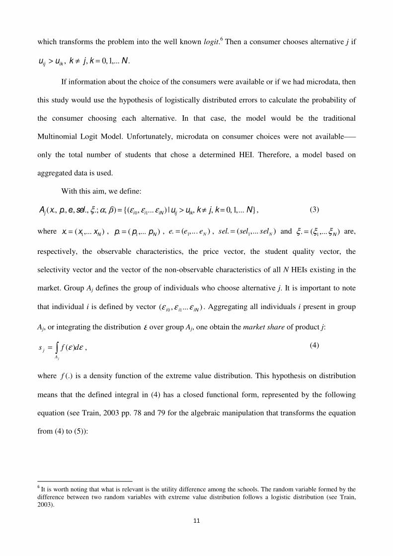
which transforms the problem into the well known logit.6 Then a consumer chooses alternative j if
Nkjkuu ikij ,...1 ,0 , , =≠> .
If information about the choice of the consumers were available or if we had microdata, then
this study would use the hypothesis of logistically distributed errors to calculate the probability of
the consumer choosing each alternative. In that case, the model would be the traditional
Multinomial Logit Model. Unfortunately, microdata on consumer choices were not available–—
only the total number of students that chose a determined HEI. Therefore, a model based on
aggregated data is used.
With this aim, we define:
Aj (x., p.,e., sel., ξ.; α, β) = {(εi 0, εi1... εiN ) | uij > uik, k ≠ j, k = 0, 1,... N} , (3)
where ) ,...(. 1 Nxxx = , ) ,...(. 1 Nppp = , e. = (e1,... eN) , sel. = (sel1,... sel
N) and ) ,...(. 1 Nξξξ = are,
respectively, the observable characteristics, the price vector, the student quality vector, the
selectivity vector and the vector of the non-observable characteristics of all N HEIs existing in the
market. Group Aj defines the group of individuals who choose alternative j. It is important to note
that individual i is defined by vector ) ... ,( 10 iNii εεε . Aggregating all individuals i present in group
Aj, or integrating the distribution ε over group Aj, one obtain the market share of product j:
εε dfs
jA
j ∫= )( , (4)
where f (.) is a density function of the extreme value distribution. This hypothesis on distribution
means that the defined integral in (4) has a closed functional form, represented by the following
equation (see Train, 2003 pp. 78 and 79 for the algebraic manipulation that transforms the equation
from (4) to (5)):
6 It is worth noting that what is relevant is the utility difference among the schools. The random variable formed by the
difference between two random variables with extreme value distribution follows a logistic distribution (see Train, 2003).
12
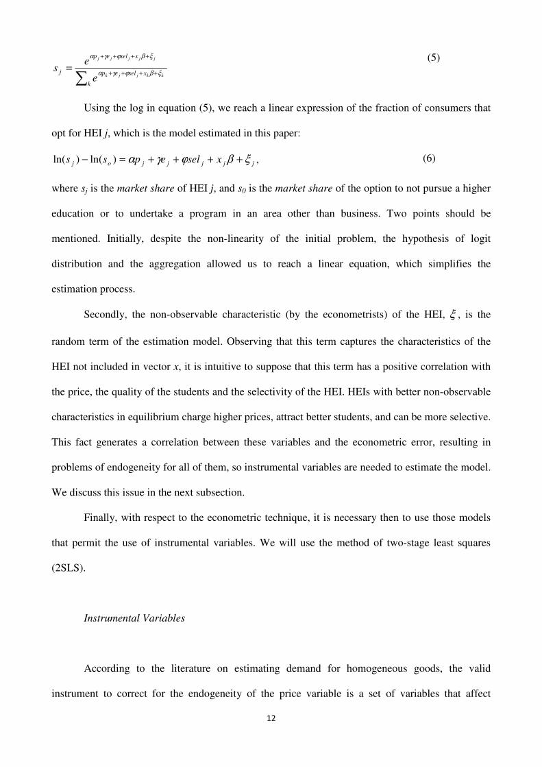
∑++++
++++
=
k
xselep
xselep
jkkjjk
jjjjj
e
es
ξβϕγα
ξβϕγα
(5)
Using the log in equation (5), we reach a linear expression of the fraction of consumers that
opt for HEI j, which is the model estimated in this paper:
jjjjjoj xselepss ξβϕγα ++++=− )ln()ln( , (6)
where sj is the market share of HEI j, and s0 is the market share of the option to not pursue a higher
education or to undertake a program in an area other than business. Two points should be
mentioned. Initially, despite the non-linearity of the initial problem, the hypothesis of logit
distribution and the aggregation allowed us to reach a linear equation, which simplifies the
estimation process.
Secondly, the non-observable characteristic (by the econometrists) of the HEI, ξ , is the
random term of the estimation model. Observing that this term captures the characteristics of the
HEI not included in vector x, it is intuitive to suppose that this term has a positive correlation with
the price, the quality of the students and the selectivity of the HEI. HEIs with better non-observable
characteristics in equilibrium charge higher prices, attract better students, and can be more selective.
This fact generates a correlation between these variables and the econometric error, resulting in
problems of endogeneity for all of them, so instrumental variables are needed to estimate the model.
We discuss this issue in the next subsection.
Finally, with respect to the econometric technique, it is necessary then to use those models
that permit the use of instrumental variables. We will use the method of two-stage least squares
(2SLS).
Instrumental Variables
According to the literature on estimating demand for homogeneous goods, the valid
instrument to correct for the endogeneity of the price variable is a set of variables that affect
13
business costs and are unrelated to demand shocks. In theory, the same type of instrument can be
utilized in markets with differentiated goods. However, there are rare situations in which cost
variables of firms are related to only one differentiated good, without being correlated with all of
the market goods. Therefore, another type of instrument should be used.
In the literature, there are two possible solutions to this problem. The first, derived by BLP,
uses the exogenous characteristics of the firm’s own product as instruments for themselves and the
sum or average of the rivals firms’ product characteristics as instruments for the price. According to
Bertrand’s oligopoly model with differentiated goods, in market equilibrium, the better the quality
of the rival goods, the lower the equilibrium price of the firm in question.
The second solution, introduced by Hausman (1996), advocates the use of the same
product’s price in another market as an instrument for the price.7 In the problem analyzed here, one
HEI is different from another, not having a product brand appearing in different markets, nor two
HEIs in different cities. This forces us to opt for the first solution, in which we use the average of
the characteristics of the other HEIs as an instrument for the price.
The quality of enrolled students and HEI selectivity are also endogenous variables. We will
use the same group of instrumental variables that we use for price: competitor characteristics, and
the age of the HEI. The age must be related to the reputation of the school, the hypothesis being that
the older HEIs are more likely to have better reputations.8
Data
The Brazilian market for HEIs is marked by the predominance of private enterprise. Among
2281 HEIs in 2006, 89% were private, and 74.6% of all university students were enrolled in these
7 For a discussion of the pros and cons of each kind of instrument, see Nevo (2001). 8 A possible explanation for the reason older schools have better reputations is based in the hypothesis that there is asymmetry of information in the HEI market, which becomes less important over time. Initially, the schools alone know the quality of their students. Over time, this quality is known not only by the alumni of the HEI but also by potential students on the market. Older schools have already revealed their true quality, and only those that reach a certain level can attract students and survive the competition.
14
private schools. Additionally, the majority of private HEIs (52%) are for profit.9 Despite the lack of
official data on the amount of donations received by HEIs, it is known that the resources derived
from this source are limited, as are the resources available to fund research. In this context,
Brazilian private HEIs primarily raise funds from student tuition payments10. The state of Sao Paulo
was chosen because 24.1% of the HEIs in the country are located there. The analysis is focused on
the area of business because it is the largest in terms of number of programs (7.6% of the total) and
number of registered students (13.9% of total students).
As mentioned in the previous section, the model represented by equation (6) will be
estimated in this work. We will explain the variables utilized in this estimation, as well as the
source of the data.
At the onset, it is important to define the dependent variable or the market share of the HEIs
(variable js in equation (6)). This is equal to the ratio between the number of students that want to
study at an HEI and the number of potential students in the market where the HEI is located.
To reach the market share denominator, it is necessary to explain a priori the markets in
which the HEI participates. In the present work, we assume, in a simplifying manner, that each
municipality with at least one business program corresponds to a market11. At the same time, to
reach the number of potential consumers of an HEI, the study takes into consideration the fact that
the consumer has completed secondary education, is between 18 and 25 years old, and is being
confronted with three possibilities: to attend a business program, to attend a higher-education
9 The source of these data on Brazilin HEIs is the Sinopse Estatística da Educação Superior do Inep (http://www.inep.gov.br/superior/censosuperior/sinopse/). 10 In contrast, data from the U.S. National Center of Education and Statistics show that 70% of the income of for-profit HEIs comes from sources other than tuition. Donations and research funds are a crucial part of their strategies and plans. 11
An alternative would be to define the market in terms of economic regions of different municipalities. However, a certain amount of arbitrariness would be necessary to define these alternative market borders. Another alternative would be to consider the city of São Paulo as more than one market because of its size. Again, it would be difficult to define the boundaries of this market. Next, we will propose models that seek to capture the specificity of the São Paulo market.
15
program in another field or to not attend a higher-education program at all.12 All of the students who
opt for one of these alternatives and who live in the municipality where the HEI is located are part
of the HEI’s potential market.
The 2006 Higher Education Census from the Ministry of Education (MEC) provides
information, by municipality, on the number of students in the first two options, the business
program or the program in another field. In addition, the 2007 Population Census carried out by the
Brazilian Bureau of Statistics (IBGE) shows that 27% of individuals between 18 and 25 years old
who have finished secondary education do attend an HEI. Therefore, knowing the number of
students in the first two groups and the participation percentage of the third group, we can estimate
the number of potential consumers, which will be the denominator of the market-share formula of
the HEI in the municipality. This number is then equal to the ratio between the number of students
enrolled in any undergraduate degree (business and others) in the municipality and 0.27.
It is difficult to define the numerator of the market-share formula of the HEI. As we
discussed in the econometric model section, we use the number of students who take the entrance
exam for the business program at an HEI13, in order to avoid the fact that in the education sector not
only the students chooses the HEI but also is chosen by it. We are aware that there is a problem
with this alternative: many students take various exams, for different HEIs, in the same year. Thus,
the average might overestimate the demand for the HEI.
A possible alternative is to use the number of registered students in the HEI business
program. The problem with this alternative is that the HEIs that are more selective, that is, that have
higher candidate/slots ratios, tend to work with excess demand. As discussed in section 2, they do
not adjust the tuition to balance the amount demanded with the amount offered. The reason, as was
already discussed, is that in the education sector, the consumer (the student) is also an input in the
12
The considered age group might omit some recently observed features. For example, the 2006 Higher Education Census, performed by the INEP, shows, for example, an increase in the participation of students in the age group of 25 to 29 years old between the years 2000 and 2006. 13
In Brazil, all applicants to a given HEI must take an entrance exam.
16
productive process. The better quality the registered students are, ceteris paribus, the better the
quality of the students educated at the HEI. This occurs in large part because students can benefit
from interacting with the other students, through what is known as the peer effect, and because the
quality of the HEI supplies a signal about the quality of the graduate in the job market after
completing higher education.14 Moreover, the HEIs with excess demand certainly would have a
better market share if they were to have a less rigorous selection process and accept more students.
Therefore, the number of registered students as a measure of the numerator for the market-share
formula underestimates the demand for the HEIs with higher selectivity. Last but not least, with this
alternative, we could not apply the models of discrete choice, as pointed out in the econometric
model section. Hence, we do not consider this alternative.
The data of the number of student applicants to each HEI comes from the 2006 Higher
Education Census of the MEC.
This study now proceeds to a discussion of the different observable characteristics related to
the variable quality of the HEIs that can affect the choice of the student and are used as explanatory
variables (variable jx in equation (6)) in the empirical model. Two variables are related to the
quality of the faculty body: the percentage of professors with doctorates (perc_doutor) and the
percentage of full-time professors (perc_int). These variables are collected from the 2005 Faculty
Body Census. At first, a high percentage of professors with doctorates and full-time professors
might signal the quality of the program; however, the business student certainly is also interested in
their professors’ business experience, which often competes with the full-time dedication of a
university professor. Therefore, whether a superior title means better academic quality in the
program (maintaining constant the rest of the variables) is questionable. For example, a professor
who is also the director of a large company may attract more candidates to a business course than a
full-time professor with a PhD degree.
14 See Winston and Zimmerman (2003) for a summary of the literature on the peer effect and MacLeod and Urquiola
(2009) on the effect of the reputation of the school on the quality of the students.
17
Other observable characteristics related to the variable quality of the HEIs used as
explanatory variables are the ones related the conditions of the infrastructure offered by the HEI.
The models in this paper consider three variables: the quality of the overall physical structure
(qual_infra), the quality of the library (qual_libr) and the availability of computers (qual_comp).
These three variables are obtained from a socioeconomic survey administered to undergraduate
students during the National Student Performance Exam (Enade), carried out by the MEC and
compiled at the 2006 Enade Census. The students grade each of these variables and an average
score for each of those is obtained. In the case of these three physical-infrastructure variables, the
signs of their coefficients are expected to be positive; that is, better infrastructure should correspond
to a greater market share.
The authors collected pricing information during the first semester of 2008. A negative sign
for the tuition coefficient is expected.
Every new undergraduate student in business (and in other programs as well) must take an
exam that encompass specific and general knowledge, the Enade. The average score of the students
in a given HEI is used in this paper as a proxy for the quality of the student body that the student
will find if he chooses this HEI. This variable comes from the 2006 Enade Census. This variable
might signify that the students take into account the effect of their peers (peer effect) in their choice
of HEI. Additionally, schools with better students have a better reputation, generating better results
for their students in the job market after graduation. In both cases, the higher the Enade score is, the
more qualified the group of students and the higher the demand for the HEI.
The selectivity variable is defined as the number of candidates divided by the number of
vacancies. On the one hand, a higher selectivity implies less likelihood that the student will be
accepted by the HEI. Hence, we expect that this variable will have a negative effect on the choice of
the student. On the other hand, this variable may be seen as another proxy for the quality of the
student body. In this regard, the higher Enade score is, the higher is the demand for the HEI.
18
Therefore, the sign of the coefficient of the variable selectivity is unclear from a theoretical point of
view.
In terms of the market (municipality) in which the HEI is located—as identified by the 2006
Higher Education Census—the model includes the GDP per capita of the municipality (GDP-pc) for
the year 2007, as obtained from Ipeadata.15 In terms of the location, a dummy variable (SP) assumes
the value one when the HEI is in the market of the capital, the city of Sao Paulo, and zero
otherwise. As the density of business programs in relation to the total population is smaller in the
capital than in other cities, an inferior market share is expected in the capital.
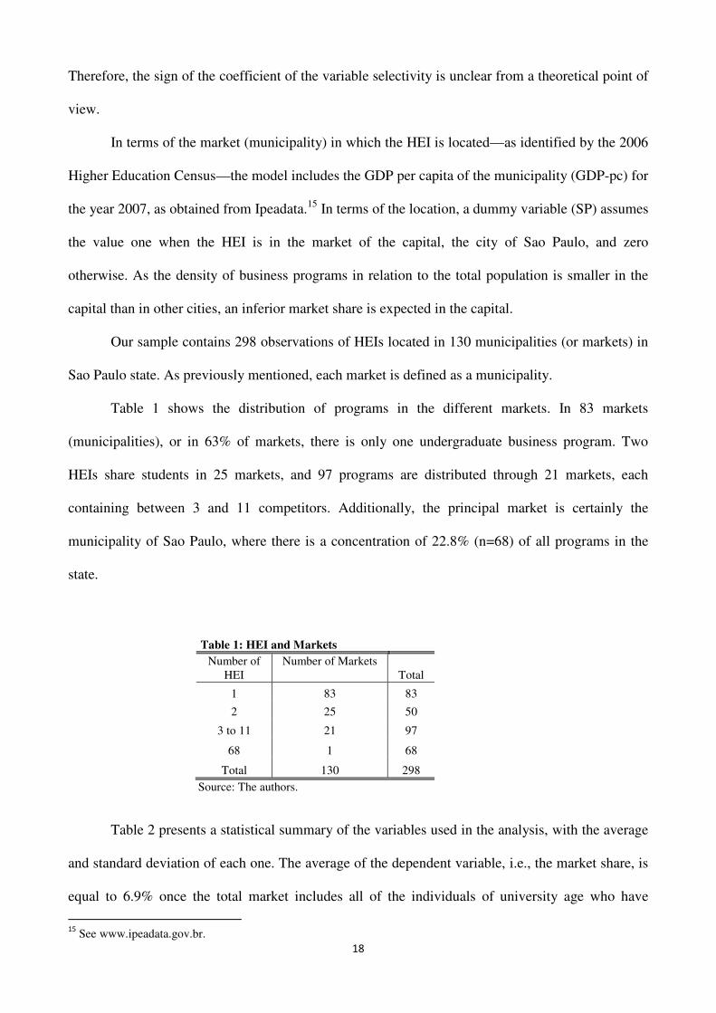
Our sample contains 298 observations of HEIs located in 130 municipalities (or markets) in
Sao Paulo state. As previously mentioned, each market is defined as a municipality.
Table 1 shows the distribution of programs in the different markets. In 83 markets
(municipalities), or in 63% of markets, there is only one undergraduate business program. Two
HEIs share students in 25 markets, and 97 programs are distributed through 21 markets, each
containing between 3 and 11 competitors. Additionally, the principal market is certainly the
municipality of Sao Paulo, where there is a concentration of 22.8% (n=68) of all programs in the
state.
Table 1: HEI and Markets
Number of HEI
Number of Markets Total
1 83 83
2 25 50
3 to 11 21 97
68 1 68
Total 130 298
Source: The authors.
Table 2 presents a statistical summary of the variables used in the analysis, with the average
and standard deviation of each one. The average of the dependent variable, i.e., the market share, is
equal to 6.9% once the total market includes all of the individuals of university age who have
15
See www.ipeadata.gov.br.
19
completed secondary school, whether enrolled in a business program or not. The HEIs are, on
average, 9.2 years old, and practically all offer a bachelor’s program rather than a technical
program.
The average Enade score of the registered students is equal to 39.5 (on a scale of 0 to 100).
Considering only the 20 programs with the highest candidate/vacancy ratios, the Enade average
rises to 44.6.
The average tuition is equal to R$ 506.85 (or US$ 318), and the municipalities’ average
GDP per capita is equal to R$ 28 750.95 (or US$ 18.082). Additionally, among the HEIs analyzed,
the average percentage of professors with doctorates and full-time professors are, respectively,
8.5% and 12.5%.
Table 2: Statistical Summary
Variable Average Standard Deviation
Mkt Share (%) 6.9 11.2
Enade Score (0-100) 39.5 4.3
Price (R$) 506.85 249.2
Professors with Doctorates (%) 8.5 9.3
Full-time Professors (%) 12.5 15.1
GDP per capita (R$) 28750.95 18200.1
Age 9.2 12.2
Bachelor’s Degree Offered (%) 94.8
Source: The authors.
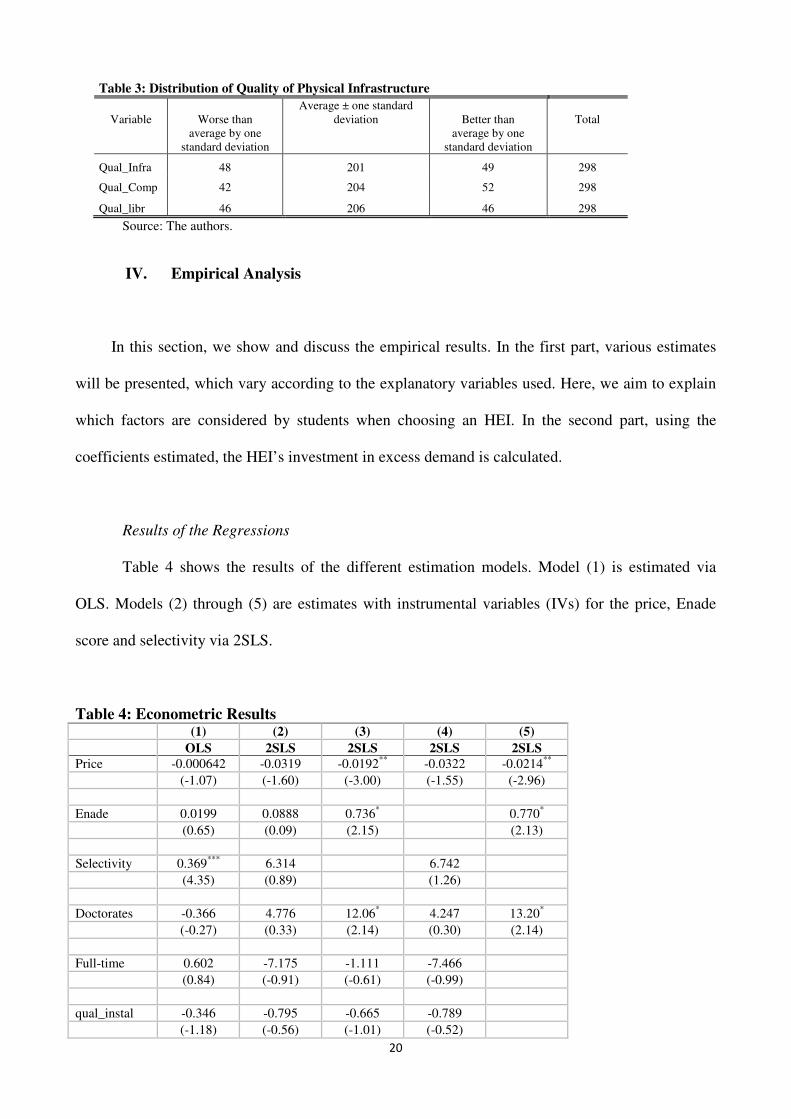
Finally, Table 3 shows the distribution of the average scores of the variables related to the
conditions of the infrastructure: the quality of the overall physical infrastructure, the library, and
computer availability. The second, third and fourth columns present the number of programs with
evaluation, respectively, ‘worse than average by one standard deviation (sd)’, ‘average ± one sd’,
and ‘better than average by one sd’.
20
Table 3: Distribution of Quality of Physical Infrastructure
Variable Worse than Average ± one standard
deviation Better than Total
average by one
standard deviation average by one
standard deviation
Qual_Infra 48 201 49 298
Qual_Comp 42 204 52 298
Qual_libr 46 206 46 298
Source: The authors.
IV. Empirical Analysis
In this section, we show and discuss the empirical results. In the first part, various estimates
will be presented, which vary according to the explanatory variables used. Here, we aim to explain
which factors are considered by students when choosing an HEI. In the second part, using the
coefficients estimated, the HEI’s investment in excess demand is calculated.
Results of the Regressions
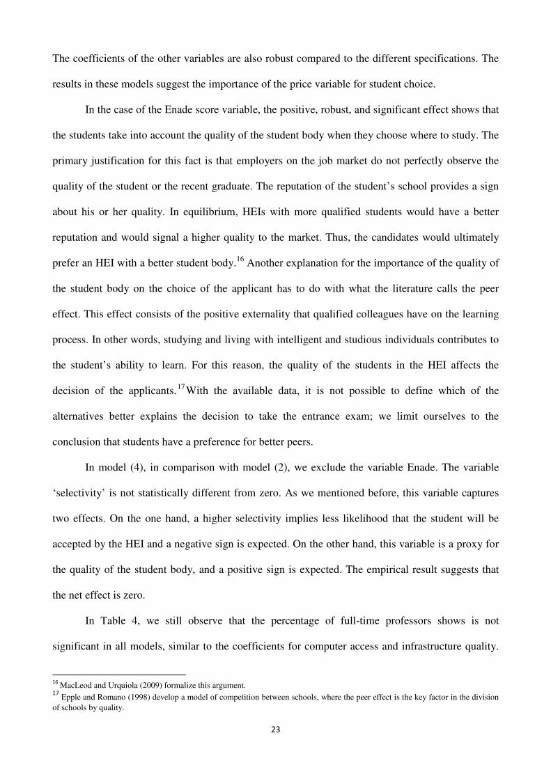
Table 4 shows the results of the different estimation models. Model (1) is estimated via
OLS. Models (2) through (5) are estimates with instrumental variables (IVs) for the price, Enade