Permanent Income Life Cycle Hypothesis Models Growth and...

Permanent Income Life Cycle Hypothesis ModelsGrowth and Development

Raul Santaeulalia-Llopis

MOVE-UAB and Barcelona GSE

Spring 2017

Raul Santaeulalia-Llopis (MOVE,UAB,BGSE) PILCH Models Spring 2016 1 / 78

1 The Model

2 Partial EquilibriumPrecautionary savings motive

A simple model and a general resultA parametric example for the general model

Liquidity constraintsThe Euler equation with liquidity constraintsLiquidity constraints with quadratic preferences (No Prudence)

Numerical solutions of models with precautionary saving and liquidity constraints(a) Infinite T =∞, value function iteration(b) Finite T , value function iteration(c) Infinite T =∞, policy function iteration on the Euler equation(d) Finite T , policy function iteration on the Euler equation

Alternative Solution Method: Endogenous Grid

3 General EquilibriumA Macroeconomic Model with Heterogeneous AgentsSequential markets equilibriumRecursive competitive equilibriumStationary recursive competitive equilibriumTheoretical results: existence and uniquenessComputation of the general equilibrium


The Model

• Permanent income - Life Cycle Hypothesis (PILCH) models assume that agents donot have access to a complete set of contingent consumption claims.

B Franco Modigliani and Albert Ando stressed the issues surrounding the finiteness oflife and planning for retirement (Life-Cycle Hypothesis).

B Friedman stressed issues surrounding income fluctuation (Permanent IncomeHypothesis).1

• We see the main difference from complete markets looking at the BudgetConstraint

ct(st) + qt(s

t)at+1(s t) = yt(st) + at(s

t−1)

where at+1(s t) is a one-period risk free IOU (I owe you) only, that is, no explicitinsurance is allowed, only self-insurance via asset accumulation.

• Notice that all variables are functions of s t but not st+1 (same payoff in all states).

1These were hypothesis about behavior, the authors never wrote a model.Raul Santaeulalia-Llopis (MOVE,UAB,BGSE) PILCH Models Spring 2016 3 / 78

• The basic income fluctuation problem with exogenous incomplete markets is then

maxc(st ),at+1(st )

T∑t=0

∑st

βtπt(st)U i (c i (s t), s t) (1)

subject to

B budget constraint

ct(st) + qt(s

t)at+1(st) = yt(st) + at(s

t−1) (2)

B a no Ponzi condition (assumed to be sufficient wide so as to never bindat the optimal allocation), normally a short-sale constraint on assets.

B an initial condition a0(s−1) = a−1.


1 The income process of the individual is stochastic and given by {yt}Tt=0

2 The preference shock affecting individuals’ preferences is a deterministic sequence{st}.

3 When T =∞ we impose a short sale constraint on IOU’s that prevents Ponzischeme, but loose enough to allow optimal consumption smoothing, and noticethat when T <∞ we do not require no Ponzi scheme condition as long as we donot allow anybody to die in debt. The short sale constraint we impose is of theform, say

at+1(s t) ≥ − supt

∞∑τ=t+1

∑sτ |sτ−1

πτ (sτ )yτ (sτ )

(1 + r)τ−(t+1)


• The problem households solve is

maxT∑t=0

∑st

βtπt(st)U i (c i (s t), s t)

s.t.ct(s

t) + qat+1(s t) = yt(st) + at(s

t−1).

• The price of a one period bond q = 11+r

is nonstochastic and constant over time.


•

maxT∑t=0

∑st

βtπt(st)U i (yt(s

t) + at(st−1)− qat+1(s t), s t)

Take first order conditions with respect to at+1(s t)

−qβtπt(st)U i

c(ct(st), s t) + βt+1

∑st+1|st

πt+1(s t)U ic(ct+1(s t+1), s t+1) = 0 (3)

that is,

U ic(ct(s

t), s t) =β

q

∑st+1 πt+1(s t+1)

πt(s t)


• That is, for each of all given pair t and s t we can also write as,

U ic(ct(s

t), s t) =

(1 + r

1 + ρ

) ∑st+1|st

πt+1(s t+1|s t)[U i

c(ct+1(s t+1), s t+1)|s t]

(4)

or more compactly,

U ic(ct , s

t) =

(1 + r

1 + ρ

)Et

[U i

c(ct+1, st+1)

]for all given pair t and s t (5)

where Et is the expectation of s t+1 conditional on s t .

• Equation (26) is the standard Euler Equation for PILCH type models.


Partial Equilibrium

B interest rate process is exogenously given (partial equilibrium)

B agents can only self-insure against income fluctuations by trading1-period risk free bonds2

• This implies relaxing 2 assumptions underlying the martingalehypothesis:

B Incorporate a precautionary saving motive into the model (relax theassumption of linear marginal utility under uncertainty) so that agentsreduce current consumption (increase savings) as reaction to anincrease of uncertainty w.r.t. future labor income (Kimball 1990 andDeaton 1991)

B Incorporate some potentially binding borrowing constraint (aliquidity constraint) that may prevent agents to borrow as much asdesired to smooth consumption over time.

2by borrowing and lending at a risk free rateRaul Santaeulalia-Llopis (MOVE,UAB,BGSE) PILCH Models Spring 2016 9 / 78

Precautionary savings motive (Prudence)

• Recall that certainty equivalence explicitly rules out precautionary saving

• The consumption function under certainty equivalence states that only the conditional (ont information) first moment of the yt+s ’s matters for the consumption choice, but not theconditional variance of future labor income.


A simple model and a general result

• 2-period model: income is know in period 0, y0, and in period 1 income is stochastic.3

• Denote Y1 the random income in period 1,

Y1 = y1 + Y1

where E0Y1 = y1 (conditional expectation) and Y1 is a random variable with E0Y1 = 0.

• Denote the expected present discounted value of lifetime labor income (with, remember,r = 0)

w = y0 + y1 (6)

3Assume also r = ρ = 0—results go through being more flexible with r and ρ butalgebra gets messy.


• Consumption at date 1 is then,

c1 = w − c0 + Y1. (7)

that is , c1 is stochastic and varies with the realization of Y1.

• The Euler equation (ignoring family size or other shocks to preferences) is

uc (c0) = E0uc (w − c0 + Y1) (8)


• We want to determine how consumption in period 0 (hence savings, s = w − c0) varieswith σ2

y = Var(Y1), the degree of uncertainty about labor income in period 1.

• For concreteness assume Y1 can take 2 values, either ε with probability 1/2 or −ε withprobability 1/2 with 0 < ε < y1 so that σ2

y = ε2.

• Totally differentiating the Euler equation w.r.t. ε we get:

ucc (c0)d c0

d ε=

1

2ucc (w − c0 + ε)

(−d c0

d ε+ 1

)+

1

2ucc (w − c0 + ε)

(−d c0

d ε− 1

)(9)


• Thus, how much consumption in period 0 varies with the degree of uncertainty aboutlabor income in period 1, d c0

d ε, is

d c0

d ε=

12

(ucc (w − c0 + ε)− ucc (w − c0 − ε))

ucc (c0) + 12

(ucc (w − c0 + ε) + ucc (w − c0 − ε))(10)

• The denominator is unambiguously negative (as u is strictly concave).

• The numerator is positive iff

ucc (w − c0 + ε)− ucc (w − c0 − ε) > 0, (11)

that is, iff uccc (c) > 0 for arbitrary ε > 0

• Thus, a sufficient (and necessary) condition for precautionary savings (increases in s dueto increases in the uncertainty of future labor income) is a strictly convex marginal utility(third derivative of utility function is positive).


• Remarks

B Kimball 1990 defines ‘prudence’ as the intensity of the precautionary savingsmotive: the “propensity to prepare and forearm oneself in the face of uncertainty”.

B Note the term prudence defines a property of the utility function that generatesprecautionary savings, but the term prudence is not precautionary savings. Wecould generate precautionary savings behavior without a prudence motive as weshall see later.

B Note that prudence is not risk aversion. Prudence (precautionary saving motive) iscontrolled by the convexity of the marginal utility while risk aversion by theconcavity of the utility function.


A parametric example for the general model

Consider a model with many periods:

• T periods.

• In general, we can say nothing about the consumption age-profile analytically. But wemay get some qualitative results under some assumptions.

• Recall the Euler equation,

uc (ct , st) =

(1 + r

1 + ρ

)Etuc (ct+1, s

t+1) (12)


• Assuming separability and CRRA utility this becomes,

1 =

(1 + r

1 + ρ

)Et

[ct+1

ct

]6−σ (13)

1 = Et

[e

ln(

( 1+r1+ρ

)(ct+1ct

)−σ)]

(14)

1 = Et

[eσ ln ct+ln(1+r)−ln(1+ρ)e−σ ln ct+1

](15)

1 = eσ ln ct+ln(1+r)−ln(1+ρ)Et [e−σ ln ct+1 ] (16)

• Now, assume ln ct+1 is normally distributed with mean µ = Et ln ct+1 and variance σ2c .4

4This requires appropriate assumptions on the underlying income process. Forinstance, for the 2-period model above this requires that the random variablez = ln(κ+ Y1) is normally distributed where κ = w − c0 is a constant.


• Now, since

Ete−σ ln ct+1 =

∫ ∞−∞

e−σue− (u−µ)2

2σ2c

√2πσc

du = e12σ2σ2

c−σEt ln ct+1 (17)

where u is a dummy argument for ln(ct+1) in the integration.

• Then, after some algebra manipulation we can write the Euler equation as,

e−σEt∆ ln(ct+1)+ln(1+r)−ln(1+ρ)+ 12σ2σ2

c = 1 (18)

• which, taking logs,

Et∆ ln(ct+1) =1

σ(ln(1 + r)− ln(1 + ρ)) +

1

2σ2σ2

c (19)

that is, CRRA utility introduces precautionary savings motive.


• and note, for comparison, that without uncertainty the Euler equation is,

1 =

(1 + r

1 + ρ

)[ct+1

ct

]−σ(20)

• That is,

∆ ln(ct+1) =1

σ(ln(1 + r)− ln(1 + ρ)) (21)


• Remark 1. Consumption does not obey certainty equivalence. CRRA utility introduces aprecautionary savings motive that tilts the consumption profile upward in expectation—consumption growth is higher in expectation in the uncertainty case.


• Remark 2. The size of precautionary savings is determined by the parameter σ controllingprudence for the CRRA utility function.


• Remark 3. All variables vt that at t help to predict the variability of future consumptionσ2c will help to predict expected consumption growth.

Example: agents with higher income (or assets) since they may be better equipped tosmooth consumption (future uncertainty) should have lower future consumption variabilityand thus, according to (14) lower consumption growth (see, for instance, Carroll (1992)).Thus, it may be flawed to run the regression,

ln(ct+1) = α1 + α2 ln ct + α3vt + εt (22)

where they interpret a statistically significant estimate of alpha3 as evidence against thePILCH model with CRRA utility.


Liquidity constraints

• So far, individuals can borrow up to the no-Ponzi scheme condition (arbitrary largeamount) assumed generous enough never to be binding.

• However, borrowing constraints seem empirically plausible and formal econometric testsindicate so (see Zeldes 1989).


The Euler equation with liquidity constraints

• Let’s assume there exists borrowing constraints, for simplicity (following Aiyagari (1994))assume at+1(st) ≥ 0—that is, agents cannot borrow at all.

• These constraints may or may not be binding, depending on the realizations of the laborincome shock, but we have to take these constraints into account explicitly when derivingthe stochastic Euler equation.

• Attach the Lagrange multiplier µ(st) to the borrowing constraint at+1(st) ≥ 0 at eventhistory st .


• FOC w.r.t. consumption today and tomorrow remain unchanged:

βtπt(st)uc (ct(s

t), st) = λ(st) (23)

βt+1πt+1(st+1)uc (ct+1(st+1, st+1) = λ(st+1) (24)

• FOC w.r.t. at+1(st+1) becomes,

λ(st)

1 + r− µ(st) =

∑st+1|st

λ(st+1) (25)

with complementary slackness conditions,

at+1(st)µ(st) ≥ 0 (26)

at+1(st)µ(st) = 0 (27)


• Combining the FOC yields,

uc (Ct(st))− µ(st)(1 + r) = β(1 + r)

∑st+1|st

βπt+1(st+1|st)uc (ct+1(st+1)) (28)

• or in short,

uc (ct) ≥1 + r

1 + ρEtuc (ct+1) (29)

=1 + r

1 + ρEtuc (ct+1) if at+1 > 0 (30)

• This Euler equation sometimes holds with inequality, depending on whether the liquidityconstraint is binding.


• Note also from the budget constraint that

ct = yt + at −at+1

1 + r(31)

≤ yt + at (32)

because of the constraint at+1 ≥ 0. Thus,

B either at+1 = 0, therefore ct = yt + at , and

uc(ct) = uc(yt + at) (33)

B or at+1 > 0, therefore ct < at + yt and thus (using strict concavity ofthe utility function)

uc(yt + at) < uc(ct) =1 + r

1 + ρEtuc(ct+1) (34)


• Hence, we can write the Euler equation compactly as

uc (ct) = max

{uc (yt + at),

1 + r

1 + ρEtuc (ct+1)

}(35)


Liquidity constraints with quadratic preferences (NoPrudence)

• With quadratic preferences the Euler Equation becomes,

−(ct − c) = max

{−(yt + at − ct),−

1 + r

1 + ρ(Etct+1 − c)

}(36)

• For simplicity assume r = ρ, then we can write the Euler equation as,

ct = min {yt + at ,Etct+1} (37)

= min {yt + at ,Et min{yt+1 + at+1,Et+1ct+2}} (38)

and so forth.


An important implication

• Suppose the variance of future income increases (say for t + 1), making more lowrealizations of yt+1 possible (and more high realizations too).

• If the set of yt+1 values for which the borrowing constraint binds becomes bigger,Et min{yt+1 + at+1,Etct+2} declines and so does ct , since in more instances the min isthe first of the 2 objects.

• That is, saving increases in reaction to increases in uncertainty about future income,because agents, afraid of future contingencies of low consumption smooth low incomeshocks via borrowing, increase their precautionary savings.


• The presence of liquidity constraints (+ risk aversion) generates precautionary savingsbehavior without the need of a prudence motive.

• Hence, when we observe increases in savings as a reaction to increased income uncertainty,this may have a preference-based interpretation (agents are prudent: uccc > 0 or aninstitution-based interpretation (credit markets prevent or limit uncontingent borrowing).


A second important implication

• In the absence of borrowing constraints we know from our previous discussion that

ct = Et(ct+s) (39)

for all s > 0. Suppose there exists an s > 0 (say, s = 1) such that for some realization ofthe income shock yt+s (with positive probability) the agent is borrowing constrained, andthus yt+s + at+s < Etct+s .

• Then, using the law of iterated expectations, ct = min{yt + at ,Etct+1} < Etct+s . Thus,even if the liquidity constraint is not binding in period t, future potential borrowingconstraints affect current consumption choices.


Numerical solutions of models with precautionary savingand liquidity constraints

• For computational purposes we want to make the problem a consumer faces recursive.

• The stochastic process governing labor income is described by a finite state, stationaryMarkov process with domain y ∈ Y = {y1, . . . , yN} and transition probabilities π(y ′|y)where we assume y1 ≥ 0 and yi+1 > yi .

• As state variables we choose current asset holdings and the current labor income shock(a, y).


Borrowing limits

• In order to make the problem well-behaved we have to make sure that agents do not gointo debt so much that they cannot pay at least the interest on that debt and still havenon-negative consumption.

• Let A be the max amount an agent is allowed to borrow.

• Since consumption equals c = y + a− a′

1+r, we have, for an agent that i) borrowed the

max amount a = −A, ii) received the worst income shock y1 and iii) just repays interest(i.e. a′ = A):

c = y1 + A−A

1 + r≥ 0 (40)

Non-negativity of consumption implies the borrowing limit,

A =1 + r

ry1 (41)

which we impose on the consumer.


• Since A is also the present discounted value of future labor income in the worst possiblescenario of always obtaining the lowest income realization y1, we may call this borrowinglimit the natural debt limit (Aiyagari 1994).

• Note that, since borrowing up to the borrowing limit implies a positive probability of zeroconsumption next period (if π(y1|y) > 0 for all y ∈ Y ), this borrowing constraint is notgoing to be binding, as long as the utility function satisfies the Inada conditions.


Bellman’s equation

• For any a ∈ [A,∞] and any y ∈ Y we then can write Bellman’s equation as,

vt(a, y) = max−A≤a′≤(1+r)(a+y)

u

(y + a−

a′

1 + r

)+ β

∑y′π(y ′|y)vt+1(a′, y ′) (42)

• The first order condition to this problem is,

1

1 + ru′(y + a−

a′

1 + r

)= β

∑y′π(y ′|y)v ′t+1(a′, y ′) (43)

where v ′t+1 is the derivative of vt+1 w.r.t. its first argument.


Euler equation

• The envelope condition is,

v ′t (a, y) = u′(y + a−

a′

1 + r

)(44)

which we can forward one period.

• Combining FOC and envelope yields,

u′(y + a−

a′

1 + r

)= β(1 + r)

∑y′π(y ′|y)u′

(y ′ + a′ −

a′′

1 + r

)(45)

• Defining ct = y + a− a′

1+rand ct+1 = y ′ + a′ − a

′′

1+rwe are back to our previously derived

stochastic Euler equation.


Computation of partial equilibrium PILCH models

• As we have seen in class previously, we can either work on the value function directly orwork on the Euler equations to solve for optimal policies.

• Also, we have seen that depending on the time horizon of the agent (finite versus infinite),different iterative procedures can be applied.


(a) Infinite T =∞, value function iteration• We want to find a time-invariant value function v(a, y) and associated policy functions

c(a, y), a′(a, y).

• We need to find a fixed point to Bellman’s equation, since there is no final period to startfrom.

• Thus, we make an initial guess for the value function v0(a, y) and then iterate on thefunctional equation,

vn(a, y) = max−A≤a′≤(1+r)(a+y)

u

(y + a−

a′

1 + r

)+ β

∑y′π(y ′|y)vn−1(a′, y ′) (46)

until it converges,‖vn − vn−1‖ ≤ εv

• Note that at each iteration we generate policy functions a′n(a, y) and cn(a, y).

• We know that under appropriate assumptions (β < 1 and u bounded), the operatordefined by Bellman’s equation is a contraction mapping and hence convergence of theiterative procedure to a unique fixed point is guaranteed.


(b) Finite T , value function iteration

• We want to find sequences of value functions {vt(a, y)}Tt=0 and associated policy

functions {ct(a, y), at+1(a, y)}Tt+0.

• Given that agent dies at period T we can normalize vT+1 ≡ 0

• Then we can iterate backwards on the equation (41): at period t we know the functionvt+1(·, ·), hence we can solve the maximization problem to find functions a′t(·, ·), vt(·, ·)and ct(·, ·).

• Note that for each t there are as many maximization problems to solve as there areadmissible (a, y)-pairs.


(c) Infinite T =∞, policy function iteration on the Eulerequation

• We have no initial period, so we guess an initial policy a′0(a, y) or c0(a, y) and theniterate on

u′(y + a−

a′tn(a, y)

1 + r

)= β(1 + r)

∑y′π(y ′|y)u′

(y ′ + a′t

n −a′t+1

n−1(a′tn(a, y), y ′)

1 + r

)

until it converges,

‖a′n − a′n−1‖ ≤ εa

• Deaton (1992) argues that under the assumption β(1 + r) < 1 the operator defined by theEuler equation is a contraction mapping, so that convergence to a unique fixed point isguaranteed.


(d) Finite T , policy function iteration on the Eulerequation

• We want to find sequences of policy functions {ct(a, y), a′t(a, y)}Tt=0. Again, given thatthe agent dies at period T + 1 we know that at period T all income will be consumed andnothing saved, thus

cT (a, y) = a + y

a′T (a, y)

• The Euler equation between period t and t + 1 reads as

u′(y + a−

a′t(a, y)

1 + r

)= β(1 + r)

∑y′π(y ′|y)u′

(y ′ + a′t(a, y)−

a′t+1(a′t(a, y), y ′)

1 + r

)

where a′t+1(a′t(a, y), y ′) is a known function from the previous step and we want to solvefor the function a′t(·, ·).

• Note that for a given (a, y) (contrary to the previous procedure, VFI) no maximization isneeded to find a′t(a, y), one just has to find a solution to a (potentially higher nonlinear)single equation. And we have learned how to do that in the first half of this course.


Simulations of time paths• Once one has solved for the policy functions one can simulate time paths (of say M

periods) for consumption and asset holdings.

• Start at some asset level a0, possibly equal to zero, then draw a sequence of randomincome numbers {yi}Mt=0 according to the specified income process.

• Now one can generate a time series for consumption and asset holdings for the infinitehorizon case by

c0 = c(a0, y0)

a1 = a′(a0, y0)

and recursively,

ci = c(ai , yi )

ai+1 = a′(ai , yi )

• The same applies for the finite horizon case, but here the policy functions also vary withtime.


What if the income process follows a random walk?

• Similar treatment to how we deal with RA models with stochastic trends.

• See Deaton’s example in Kruger’s notes.


Alternative Solution Method: Endogenous grid

• Chris Carroll (2008) idea: Construct a grid on a′, next period’s asset holdings, rather thanon a —as standardly done.

• Necessary condition: policy function must be at least weakly monotonic in current assets.


A model

• Recursively, agents solve

V (a, y) = maxa′

u(c) + βEtV (a′, y ′)

subject to

c + a′ ≤ y + (1 + r)a

a′ ≥ amin


• With a discrete income process we can write the Euler equation as,

uc (c(a, y)) ≥ β(1 + r)∑y′∈Y

π(y ′|y)uc (c(a′, y ′))

subject to

c + a′ ≤ y + (1 + r)a

a′ ≥ amin

• Equality holds if a′ > amin


• We want to find an invariant decision rule c(a, y) (hence a′(a, y)) that satisfies the Eulerequation and that does not violate the borrowing constraint.

• We will use Euler equation methods, iterating on the decision rule. For mere expositionpurposes, think of a descretization of the decision rule but continuous methods apply aswell.


The algorithm

• Step 1. Construct a grid on (a′, y) where a′ ∈ GA = {a1, . . . , amax} with a1 = amin andy ∈ Gy = {y1, . . . , yN}. Important: we are defining our grid over assets tomorrow.


• Step 2. Guess a decision rule c0(ai , yj ).

For example, guess a′0(a, y) = 0, that is, c0(ai , yj ) = (1 + r)ai + yj .


• Step 3. For any pair {a′i , yj} on the mesh GA × Gy construct the RHS of the Eulerequation,

RHS(a′i , yj ) = β(1 + r)∑y′∈Y

π(y ′|yj )uc (c0(a′i , y′))


• Step 4. Use the Euler equation to solve for the value c(a′i , yj ) that satisfies

uc (c(a′i , yj )) = RHS(a′i , yj )

which can be done analytically. For example, for uc (c) = c−γ we have:

c(a′i , yj ) =[RHS(a′i , yj )

]− 1γ .

This is the step that makes the algorithm more efficient:

B We do not require a nonlinear equation solver, andB We only compute the expectation in Step 3 once.


• Step 5. From the budget constraint, solve for a(a′i , yj ) such that

c(a′i , yj ) + a′i = (1 + r)a(a′i , yj ) + yj

B Where a(a′i , yj ) is the value of assets today that would lead the consumer to have a′iassets tomorrow if this income shock was yj today.

B Note this function is not necessarily defined on the grid points of GA.

B This is the endogenous grid and it changes on each iteration.

B This way, a(a′min, yj ) is the value for current assets that induces the borrowingconstraint to bind next period, i.e., a′i = amin.


• Step 6. Update the guess. To get the new guess c1(ai , yj ):

For each yj ,

B If ai > a(a′min, yj ), use some interpolation methods on the two most adjacent values{an(ai , yj ), an+1(ai , yj )} that include the given grid point ai .

B If ai < a(a′min, yj ), use the budget constraint

c1(ai , yj ) = (1 + r)ai + yj − a′min

since we cannot use the Euler equation because the borrowing constraint is binding.


• Step 7. Check convergence and stop when

maxi,j{|cn+1(a′i , yj )− cn(a′i , yj )|} < ε

If convergence is not achieve, go back to Step 3.


General Equillibrium

• Now we are ready for a fully-fledged Macroeconomic Model with Heterogeneous agents.

• This is the General Equilibrium version of PILCH models introduced in previous sessions.

• General Equilibrium implies that aggregate prices wt and rt are determined endogenously

within the model.

B It imposes theoretical discipline. The relationship between ρ and r will obey anequilibrium —rather than being arbitrarily chosen.

B It generates an endogenously determined consumption and wealth distribution andhence provides a theory of wealth inequality —that is, it provides a theoreticalframework potentially able to account for stylized facts of empirical wealthdistributions.

B It enables meaningful policy experiments. Partial equilibrium models (small openeconomies) with w and r may over- or underestimate the full effects of reforms.


A Macroeconomic Model with Heterogeneous Agents

• The economy is populated by a continuum of measure 1 of individuals that all face anincome fluctuation problem as described previously.

• Each individual is subject to the same stochastic labor endowment process {yt} withyt ∈ Y = {y1, y2, . . . , yN} —each individual will face potentially different realizations ofthis process.

• Individual labor income at t is wtyt where wt is the real wage per unit of labor. Hence, yt ,can be interpreted as the number of efficiency units of labor a household can supply in agiven time period.


• The labor endowment process is assumed to follow a stationary Markov process. Letπ(y ′|y) denote the probability that tomorrow’s endowment takes the value y ′ if today’sendowment takes the value y .

• Not only π(y ′|y) is the probability of a particular agent of a transition from y to y ′ butalso, by the law of large numbers5 the deterministic fraction of the population that hasthis particular transition.

• Let Π be the stationary distribution associated with π, assumed to be unique.

5See Uhlig (1996)


• Assume that at t = 0 the income of all agents, y0, is given, and that the distribution ofincomes across the population is given by Π. Then the distribution of income in all futureperiods is also given by Π, in particular, the total labor endowment in the economy (inefficiency units) is given by:

L =∑y

yΠ(y)

• Hence, although there is substantial idiosyncratic uncertainty about a particularindividual’s labor endowment and hence labor income is constant over time, that is, thereis no aggregate uncertainty.

• Denote πt(y t |y0) denote the probability of event history y t , given initial event y0. Then,

πt(yt |y0) = π(yt |yt−1)π(yt−1|yt−2) . . . π(y1|y0)


• Each agent’s preferences over stochastic consumption processes are given by

E0

∞∑t=0

βtu(ct)

with β = 11+ρ

and ρ > 0.

• The agent can self-insure against idiosyncratic labor endowment shocks by purchasing atperiod t uncontingent claims to consumption at period t + 1. Then, agent’s budgetconstraint is6

ct + at+1 = wty + t + (1 + rt)at

• We impose an exogenous borrowing constraint on asset holdings: at+1 > 0, that is, ano-borrowing constraint, as in the Aiyagari’s (1994) applications.

• Given (a0, y0).

6Note that instead of zero coupon bonds being traded at a discount q = 1

1+rwe now consider a bond that trades at price

1 today and earns gross interest rate (1 + rt+1) tomorrow. Three remarks: the latter option seems more suitable now becausethe asset being traded will be physical capital with the interest rate being determined by the marginal product of capital: as longas the interest rate is constant as in Aiyagari (1994) both formulations are equivalent (identical Euler equations): and, withaggregate uncertainty as in Krusell and Smith (1998), however, it would make a substantial difference whether agents can tradea risk free bond or, as Krusell and Smith assume, risky capital.


• Some notation,

B Let ct(a0, y t) and at+1(a0, y t) denote, respectively, consumption and asset holdingsat period t after endowment shock history y t is realized.

B Let Φ0(a0, y0) denote the initial measure over (a0, y0) across households.

B Let the marginal distribution of Φ0 with respect to y0 be Π.

B At each point in time each agent is characterized by her current asset position atand her current income yt . Those are agent’s individual state variables.

B The aggregate state of the economy is the cross-sectional distribution overindividual characteristics Φt(at , yt).


• On the production side:

B Assume competitive market taken factor prices as given. All firms have access to astandard neoclassical production technology,

Yt = F (Kt , Lt)

where F ∈ C2 has CRS and positive but diminishing marginal products with respectto both production factors. Inada conditions also hold.

B Firms choose labor inputs and capital inputs to maximize the present discountedvalue of profits.

B Remember that with CRS and perfect competition the number of firms isindeterminate and w/o loss of generality we can assert the existence of a singlerepresentative firm.


• The only asset in this economy is the physical capital stock, hence, in equilibrium theaggregate capital stock Kt has to equal the sum of asset holdings of all individuals, thatis, the integral over the at ’s of all agents.

• Capital depreciates at rate 0 < δ < 1.

• The aggregate resource constraint is then

Ct + Kt+1 = F (Kt , Lt) + (1− δ)Kt

where Ct is aggregate consumption at t.


• We are now ready for the definition of an equilibrium. We will look at three definitions:

B Sequential markets equilibrium: to compare this model to the complete marketsone.

B Stationary recursive equilibrium: what we will learn to compute numerically.

B Recursive equilibrium: that generalizes the stationary one, and it is what is neededwhen we introduce aggregate uncertainty.


Definition (Sequential markets equilibrium, SME)Given Φ0, a sequential markets competitive equilibrium is allocations for households{ct(a0, y t), at+1(a0, y t)}∞

t=0,y t∈Y , allocations for the representative firm {Kt , Lt}∞t=0 and prices

{wt , rt}∞t=0 such that,

1 Given prices, allocations maximize agent’s problem subject to agent’s budget constraint,the nonnegativity constraints on assets and consumption and the borrowing constraint.

2 Firms maximize their profits (factor prices equate marginal productivities),

rt = FK (Kt , Lt)− δwt = FL(Kt , Lt)

3 Forall t, markets clear, respectively assets, labor and goods:

Kt+1 =

∫ ∑y′∈Y

at+1(a0, yt)π(y t |y0)dΦ0(a0, y0)

Lt = L =

∫ ∑y′∈Y

YTπ(y t |y0)dΦ0(a0, y0)

∫ ∑y′∈Y

ct(a0, yt)π(y t |y0)dΦ0(a0, y0) + Kt+1 = F (Kt , Lt) + (1− δ)Kt


• Let’s define the recursive competitive equilibrium.

• First, we need to define a measurable space on which the measure Φ are defined.

B Define the set A = [0,∞) of possible asset holdings and the set Y of possible laborendowment realizations.

B Define by P(Y ) the power set of Y (i.e. the set of all subsets of Y ) and by B(A)the Borel σ-algebra of A.

B Let Z = A× Y and B(Z) = P(Y )× B(A).

B Define M the set of all probability measures on the measurable spaceM = (Z ,B(Z)).

B Why all this? Because measures Φ will be required to be elements of M.


Household problem in recursive formulation

• In recursive formulation,

v(a, y ; Φ) = maxc≥0,a′≥0

u(c) + β∑y′∈Y

π(y ′|y)v(a′, y ′; Φ′)

s.t. c + a′ = w(Φ)y + (1 + r(Φ))a

Φ′ = H(Φ)

where the function H :M→M is called the aggregate “ law of motion”.

• Note we must include all state variables in the household problem, in particular theaggregate state variable, since the interest rate r will depend on Φ.


Definition (Recursive competitive equilibrium, RCE)

A RCE is a value function v : Z ×M→ R, policy functions for the agent a′ : Z ×M→ R andc : Z ×M→ R, policy functions for the firm K :M→R and L :M→R, pricing functionsw :M→R and r :M→R and an aggregate law of motion H :M→M such that

1 Given w and r , v , a′ and c are measurable with respect to B(Z), v satisfies thehousehold’s Bellman equation and a′ and c are the associated policy functions

2 K , L satisfy, given w and r ,

r(Φ) = FK (K(Φ), L(Φ))− δ and w(Φ) = FL(K(Φ), L(Φ))

3 Markets clear. For all Φ ∈M,

K(H(Φ)) =

∫a′(a, y ; Φ) dΦ

L(Φ) =

∫y dΦ∫

c(a, y ; Φ)dΦ +

∫a′(a, y ; Φ)dΦ = F (K(Φ), L(Φ)) + (1− δ)K(Φ)

4 The aggregate law of motion H is generated by the exogenous Markov process π and thepolicy fucntion a′ (as described below).


• What does it mean that H is generated by π and a′?

B H basically tells us how a current measure over (a, y) translates into a measure Φ′

tomorrow.

B So H summarizes how individuals move within the distribution over assets andincome from one period to the next.

B But that is exactly what a transition function tells us. Define the transition functionQΦ : Z × B(Z)→ [0, 1p] by7

QΦ((a, y), (A,Y)) =∑y′∈Y

π(y ′|y) if a′(a, y ; Φ) ∈ A, 0 else

for all (a, y) ∈ Z and all (A,Y) ∈ B(Z).

B QΦ(A,Y) is the probability that an agent with current assets a and current incomey ends up with assets a′ in A tomorrow and income y ′ in Y tomorrow.

7Since a′ is a function of Φ,Q is also implicitly a function of Φ.Raul Santaeulalia-Llopis (MOVE,UAB,BGSE) PILCH Models Spring 2016 69 / 78

• How does the function QΦ help us to determine tomorrow’s measure over (a, y) fromtoday’s measure?

B Suppose QΦ were a Markov transition matrix for a finite state Markov chain and Φt

would be the distribution today.

B Then, to figure out the distribution Φt+1 tomorrow we would just multiply Q by Φt ,

Φt+1 = QTΦ Φt

where T is the transposition operator.

B But a transition function is just a generalization of a Markov transition matrix touncountable state spaces. Hence, we need integrals:

Φ′(A,Y) = H(Φ)(A,Y) =

∫QΦ((a, y), (A,Y)) Φ(da× dy)

B The fraction of people with income in Y and assets in A is the fraction of peopletoday, as measured by Φ, that transit to (A,Y), as measured by QΦ.


• In general, there is no presumption that tomorrow’s measure Φ′ equals today’s measure,since we posed an arbitrary initial distribution over types, Φ0.

• If the sequence of measures {Φt} generated by Φ0 and H is not constant, then:

B obviously interest rates r = r(Φt) are not constant,B decision rules vary with Φt over time.

• That is, the computation of equilibria is difficult in general. We would have to computethe function H explicitly, mapping measures (i.e. infinite-dimensional objects) intomeasures. We will discuss that next week. Today we will be interested in stationaryversions where Φ is constant.


Definition (Stationary recursive competitive equilibrium)

A stationary RCE is a value function v : Z →R, policy functions for the agent a′ : Z →R andc : Z →R, policies for the firm K and L, prices w and r and a measure Φ ∈M such that

1 Given w and r , v , a′ and c are measurable with respect to B(Z), v satisfies thehousehold’s Bellman equation and a′ and c are the associated policy functions.

2 K , L satisfy, given w and r ,

r = FK (K , L)− δ and w = FL(K , L)

3 Markets clear,

K =

∫a′(a, y) dΦ

L =

∫y dΦ∫

c(a, y)dΦ +

∫a′(a, y) dΦ = F (K , L) + (1− δ)K

4 For all (A,Y) ∈ B(Z),

Φ(A,Y) =

∫Q((a, y), (A,Y)) dΦ


• Note the simplification with respect to the previous nonstationary problem: valuefunctions, policy functions and prices are not any longer indexed by measures Φ.

• The last requirement states that the measure Φ reproduces itself:starting with measure over incomes and assets Φ today, generates the samemeasure tomorrow.

• In this sense, the stationary RCE is the equivalent of a steady state, only that theentity characterizing the steady state is not a number but a complicatedinfinite-dimensional object, a measure.


Theoretical results: existence and uniqueness

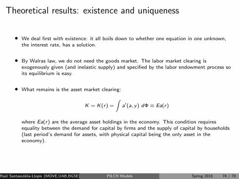
• We deal first with existence: it all boils down to whether one equation in one unknown,the interest rate, has a solution.

• By Walras law, we do not need the goods market. The labor market clearing isexogenously given (and inelastic supply) and specified by the labor endowment process soits equilibrium is easy.

• What remains is the asset market clearing:

K = K(r) =

∫a′(a, y) dΦ ≡ Ea(r)

where Ea(r) are the average asset holdings in the economy. This condition requiresequality between the demand for capital by firms and the supply of capital by households(last period’s demand for assets, with physical capital being the only asset in theeconomy).


• It is clear that capital demand K(r) is a function of r alone,

r = FK (K(r), L)− δ

since labor supply L = L > 0 is exogenous.

• Further, we know from the assumptions on the production function that K(r) is acontinuous, strictly decreasing function on r ∈ (−δ,∞) with

limr→−δ

K(r) = ∞

limr→∞

K(r) = 0


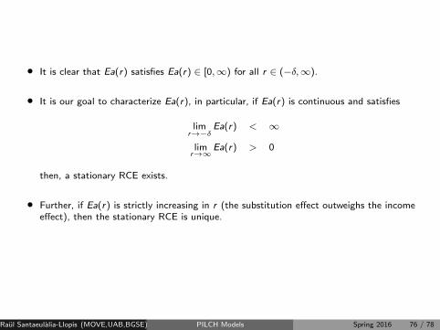
• It is clear that Ea(r) satisfies Ea(r) ∈ [0,∞) for all r ∈ (−δ,∞).

• It is our goal to characterize Ea(r), in particular, if Ea(r) is continuous and satisfies

limr→−δ

Ea(r) < ∞

limr→∞

Ea(r) > 0

then, a stationary RCE exists.

• Further, if Ea(r) is strictly increasing in r (the substitution effect outweighs the incomeeffect), then the stationary RCE is unique.


Computation of the general equilibrium

• Use your partial equilibrium programs from before (with liquidity constraints) to computethe general equilibrium for the aggregate economy.

• The algorithm goes like this:


Computational Algorithm for General Equilibrium1 Guess an interest rate r ∈ (δ, ρ).

2 Use the first order conditions for the firm to determine K(r) and w(r).

3 Solve the household problem for given r and w(r): Here you will use code of the previousexercises.

4 Use the optimal decision rule a′(a, y) together with the exogenous Markov chain π to findan invariant distribution Φt associated with a′(a, y) and π. For this you better first checkthat a′(a, y) intersects the 45-degree line for a large enough. Note that if you havediscretized the state space for assets, finding Φr amounts to finding the eigenvector(normalized to length one) associated with the largest eigenvalue of the transition matrixQ generated by a′(a, y) and π.

5 Compute

Ea(r) =

∫a′(a, y)dΦr

Again, if you have discretized the state space, the integral really is a sum.

6 Computed(r) = K(r)− Ea(r)

If d(r) is close enough to zero, you have found a stationary recursive equilibrium, if not,update your guess for r going back to (1).


Date post:	15-Mar-2020
Category:	Documents
Upload:	others
View:	16 times
Download:	0 times

Permanent Income Life Cycle Hypothesis Models Growth and...

Documents