Design of Permanent Multipole Magnets with Oriented Rare Earth Cobalt Materials

By Klaus Halbach, Lawrence Berkeley Laboratory, University of California, Berkeley, CA 94720

By taking advantage of both the magnetic strength and the astounding simplicity of the magnetic properties of oriented rare earth cobalt material, new designs have been developed for a number of devices. In this article on multi pole magnets, special emphasis is put on quadrupoles because of their frequent use and because the aperture fields achievable 1.2 1.4 T are rather large. This paper also lays the foundation for future papers on:

a Linear arrays for use as “plasma buckets” or undulators for the production of synchrotron radiation.

b Structures for the production of solenoidal fields.

c Three dimensional structures such as helical undulators or multipoles.

IntroductionFor some applications, the most important of the many advantages of permanent magnets is the fact that they can be made very small without reduction of magnetic field strength. In conventionally powered magnets, the current density in the coils is inversely proportional to the linear dimension, leading to insurmountable cooling problems and attendant reduction of field strength as size decreases.

We will discuss new designs that with the currently available oriented rare earth cobalt REC material, produce in some devices, fields that are as strong or stronger than those achievable with conventional magnets of any size.

Thus, REC magnets will have a performance advantage over conventional magnets regardless of size, shifting the decision between the two to di erent areas, such as convenience of strength adjustment, price, etc.

The advantage of REC is not only its strength, but also the simplicity of its magnetic properties. This simplicity makes REC systems easy to understand and to treat analytically, which in turn leads directly to improved designs. For this reason, we devote some space to REC

properties, and how they can be best described in the magnetostatic equations, despite the fact that these properties have been known by workers in the field since Strnat1 started the development of REC.

For the sake of completeness, we include similarly the derivation of some theorems that are, at least in principle, textbook material, but are used so infrequently that they cannot be expected to be at the fingertips of most readers.

2. Basic Formulae, NotationFor three dimensional 3D calculations, we use the standard Cartesian coordinates x, y, . Most of the two dimensional 2D calculations are done with complex numbers that are identified by underlining the symbols.

Specifically z is defined by z = x + iy =reiφ, with i2 = 1.

The complex conjugate of a quantity is indicated by an asterisk.

In a vacuum region, the two dimensional field components Bx, By or Hx, Hy can be derived from either a scalar potential V or a vector potential that only needs to have a component A in the direction:

Bx =A

y=

V

x1a

By =A

x=

V

y1b

The relationships between the derivatives of A and V are the same as the Cauchy Riemann conditions of the real and imaginary part of an analytical function of the

complex variable z , i.e., the complex potential

F z( ) = A + iV is such a function, and if we use

Nuclear Instruments and Methods 169 1980 pp. 1 10, doi:10.1016/0029 554X 80 90094 4 1

B = Bx + iBy to describe the two dimensional vector B, it

follows from equation 1 that

B* =idF

dz2

is also an analytical function of z . The field at location

z0 , generated by a current filament, I, at location z , is

given by

B* z0( ) =μ0I

2 i

1

z0 z3

The coe cients of the Taylor series expansion of F and

B* are in the customary fashion identified by the sub

script of the expansion of F :

F z0( ) = ann=1

z0n

4a

B* z0( ) = bnn=1

z0n 1;bn = inan 4b

The same expansions, but with < 0, will be used to describe fields in the region radially outside the magnets. MKS units are used throughout, with μo = 4 x 10 7 V s A 1 m 1.

3. Properties of REC 3.1. The Manufacturing Process

To get a rough understanding of the reasons for the REC properties described in section 3.2, we describe very briefly the major steps in one of the major manufacturing processes used today to produce REC. For details, the reader is referred to the book by McCaig.2

After a molten mixture of roughly five atomic parts cobalt to one atomic part of some rare earth metal s is solidified by rapid cooling, a crushing and milling process produces a powder that consists of particles with linear dimensions of the order of 5 μm. These grains are magnetically highly anisotropic, “wanting” to be polarized only along one crystalline direction. The powder is then exposed to a strong magnetic field and subjected to high pressure, causing the individual grains to physically rotate until their magnetically preferred axes are parallel to the applied field. These aligned blocks of material are then sintered, and machined or ground if necessary. Finally the material is exposed to a very strong magnetic field in a direction parallel or antiparallel to the previously established preferred direction, orienting practically all alignable magnetic moments along the direction

of magnetization, commonly called the easy axis. The property that makes REC so valuable is that this magnetization is very strong, and that it can be changed in a substantial way only by applying a strong field in the direction opposite to the one used to magnetize the material.

3.2. THE B H RELATIONSHIP OF REC

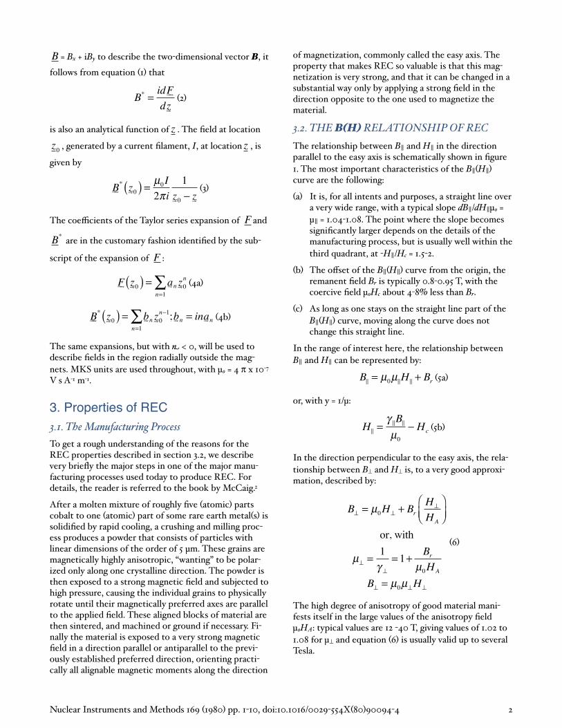
The relationship between B and H in the direction parallel to the easy axis is schematically shown in figure 1. The most important characteristics of the B H curve are the following:

a It is, for all intents and purposes, a straight line over a very wide range, with a typical slope dB /dH μo = μ = 1.04 1.08. The point where the slope becomes significantly larger depends on the details of the manufacturing process, but is usually well within the third quadrant, at H /Hc = 1.5 2.

b The o set of the B H curve from the origin, the remanent field Br is typically 0.8 0.95 T, with the coercive field μoHc about 4 8 less than Br.

c As long as one stays on the straight line part of the B H curve, moving along the curve does not change this straight line.

In the range of interest here, the relationship between B and H can be represented by:

B = μ0μ H + Br 5a

or, with y = 1/μ:

H =B

μ0Hc 5b

In the direction perpendicular to the easy axis, the relationship between B and H is, to a very good approximation, described by:

B = μ0H + BrH

HA

or, with

μ =1

= 1+Br

μ0HA

B = μ0μ H

6

The high degree of anisotropy of good material manifests itself in the large values of the anisotropy field μoHA: typical values are 12 40 T, giving values of 1.02 to 1.08 for μ and equation 6 is usually valid up to several Tesla.

Nuclear Instruments and Methods 169 1980 pp. 1 10, doi:10.1016/0029 554X 80 90094 4 2

Aside from the REC material discussed so far, resin bonded REC material is also available, with qualitatively the same properties, but lower values of Br and Hc. Some of the oriented ferrites also have similar properties, but with Br 0.35 T and larger values 1.1 for the permeabilities μ and μ .

Br

B

H�0

Hc�0�

Figure 1 — B(H)-curve in the direction parallel to the easy axis.

The designs discussed in this paper can also be implemented with these materials; we always refer to REC magnets because it is the unique strength of the REC materials, combined with the other properties described in this section, that will open the door to new and exciting applications.

3.3. Description of REC Properties in the Magnetostatic Equations

Equations 5a and 6 can be combined into the vector equation:

B = μ0μ *H + Br 7a

In this equation, Br is the vector with the magnitude of the remanent field Br in the direction of the easy axis, and μ * H = μ H +μ H . Equations 5b and 6 can be similarly combined into

H =*B

μ0Hc 7b

If we derive H from a scalar potential, we have to satisfy div B = 0, yielding with equation 7a

div μ0μ *H( ) = = divBr 8a

If we derive B similarly from a vector potential, we get from equation 7b and Amperes law

curl*B

μ0

= j = curl Hc 8b

The anisotropy of the material shows up in two di erent ways: in the inhomogeneous terms on the right sides of equations 8a, b , and in the slight anisotropy associated with the weak di erential permeability of REC. Because the permeabilities are so close to one, we assume, unless stated otherwise, that μ = μ = 1. This very good approximation, together with the assumption of constant Hc and Br means that the material can be treated as vacuum with either an imprinted charge density div Br or an imprinted current density curl Hc. This in turn has the consequence that the fields produced by di erent pieces of REC superimpose linearly, and that they can be calculated with fairly little e ort when no soft magnetic material is present. It should be noted that in the case of homogeneously magnetized material, i.e., Hc, Br = constant within the material, curl Hc and div Br are zero everywhere except at the surface, where one encounters delta functions that signify the presence of current sheets or charge sheets.

3.4 Calculation of Three Dimensional 3D Fields Produced by REC

In the absence of soft material, we derive the field at the location outside the material from a scalar potential,

H r0( ) = grad V 9

with V given by an integral over the volume of the material:

μ0V r0( ) =1

4

r( )r r0

dv 10

In the case of a homogeneously magnetized REC piece, one has a charge sheet at its surface. With equation 8a one therefore obtains in that case V from an integral over the surface of the material:

V =1

4

Hc • da

r r0=Hc

4

da

r r011

For our model, Br = μoHc has been used. A particularly appealing property of this formula is the fact that the integral is independent of Hc.

For the case of continuously varying Hc we use, with K r = 1/|r r0| the identity

K

μ0

= K div Hc = Hcgrad K div KHc( ) 11b

Because Hc = 0 outside the material,

div KHc( )dv = KHc • da = 0 11c

With grad K = r ro /|r ro|3 we obtain

Nuclear Instruments and Methods 169 1980 pp. 1 10, doi:10.1016/0029 554X 80 90094 4 3

V =1

4

Hc • r r0( )

r r03 dv 12

3.5. Calculation of Two Dimensional 2D Fields Produced by REC

For a REC assembly that is su ciently long in the zdirection and whose magnetization vector Br has no component, the fields outside the material can, in the absence of soft steel, to a good approximation be described by:

B* z0( ) =μ0

2 i

j

z0 zdxdy 13

with

μ0 j =Bryx

Brxy

14

We have again used Br = μoHc

It is shown in the Appendix that equation 13 can without restrictions on Br = Brx + i Bry, be written as

B* z0( ) =1

2

Br

zc z( )2 dxdy 15

This formula can be considered the 2D equivalent of equation 12 , because it expresses the field by an integral that contains the magnetization itself, and not a combination of its spatial derivatives.

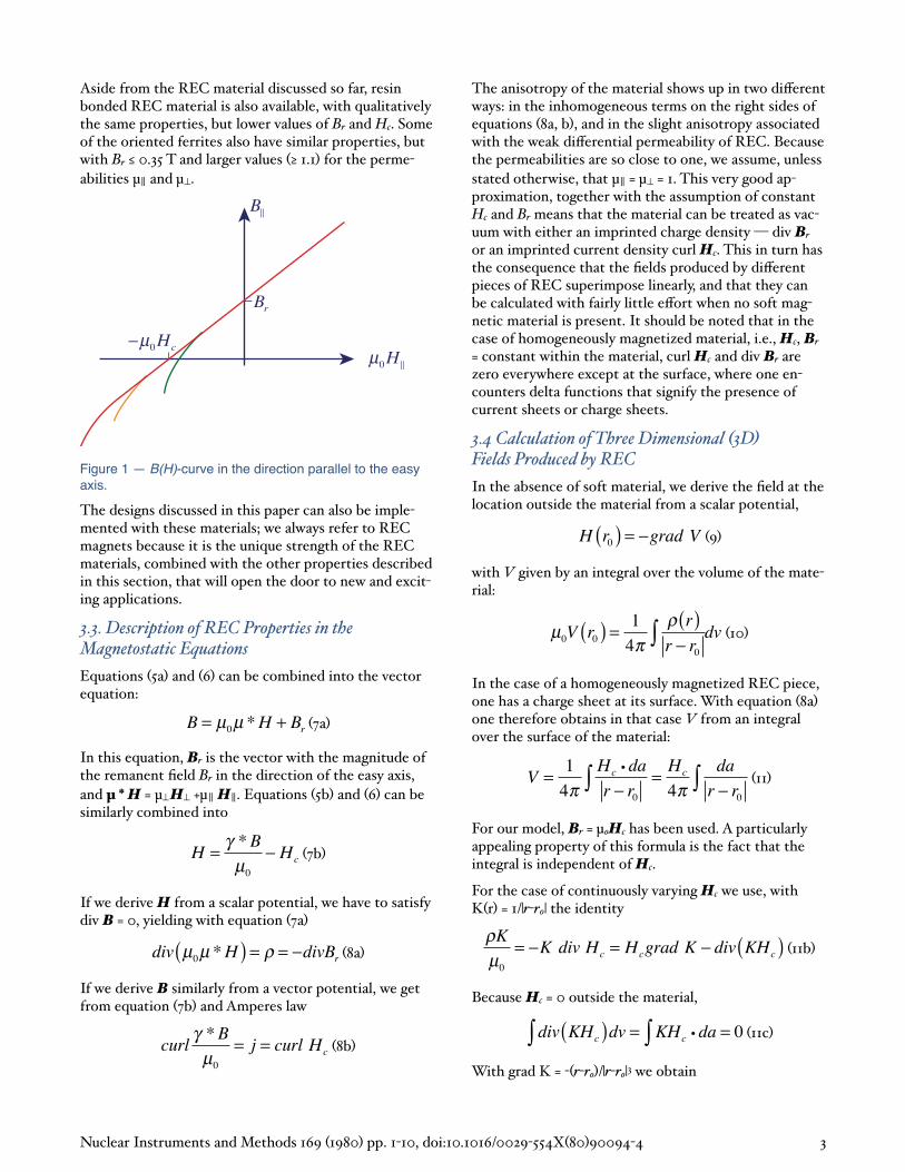
Equation 15 has a property that is highly significant for many applications: if two REC assemblies are identical, except that in the second system the easy axis is rotated everywhere by the angle + relative to the easy axis orientation in first system, then the right hand side of equation 15 for the second system equals that of the

first system, but is multiplied by ei . This allows us to state the Easy Axis Rotation Theore If in a 2D, softsteel free, REC system all easy axes are rotated by the angle + , then all magnetic fields outside the REC rotate by the angle without a change in amplitude. Figure 2 illustrates this theorem. The theorem is qualitatively easy to understand if one realizes that each volume element of REC produces a dipole field for which this theorem is valid for obvious reasons.

For a homogeneously magnetized piece of REC, Br can

be taken outside the integral in equation 15 . Integrating first over x, one obtains:

B* z0( ) =Br

2

dy

z0 z16a

Integration over y first yields

B* z0( ) =Br

2

dx

z0 z16b

and equations 16a and 16b can be combined into

B* z0( ) =Br

4 i

dz*

z0 z16c

The last three equations are given because, depending on the geometrical shape of the REC piece, one of these integrals may be easier to evaluate than the others or the integral in equation 15 .

Equation 16b and similarly equation 16a can also be derived by using the current sheet model for a REC piece with its easy axis parallel to the x axis, and then invoking the easy axis rotation theorem.

Br

B

Br

Figure 2 — Effect of rotation of easy axes on magnetic field.

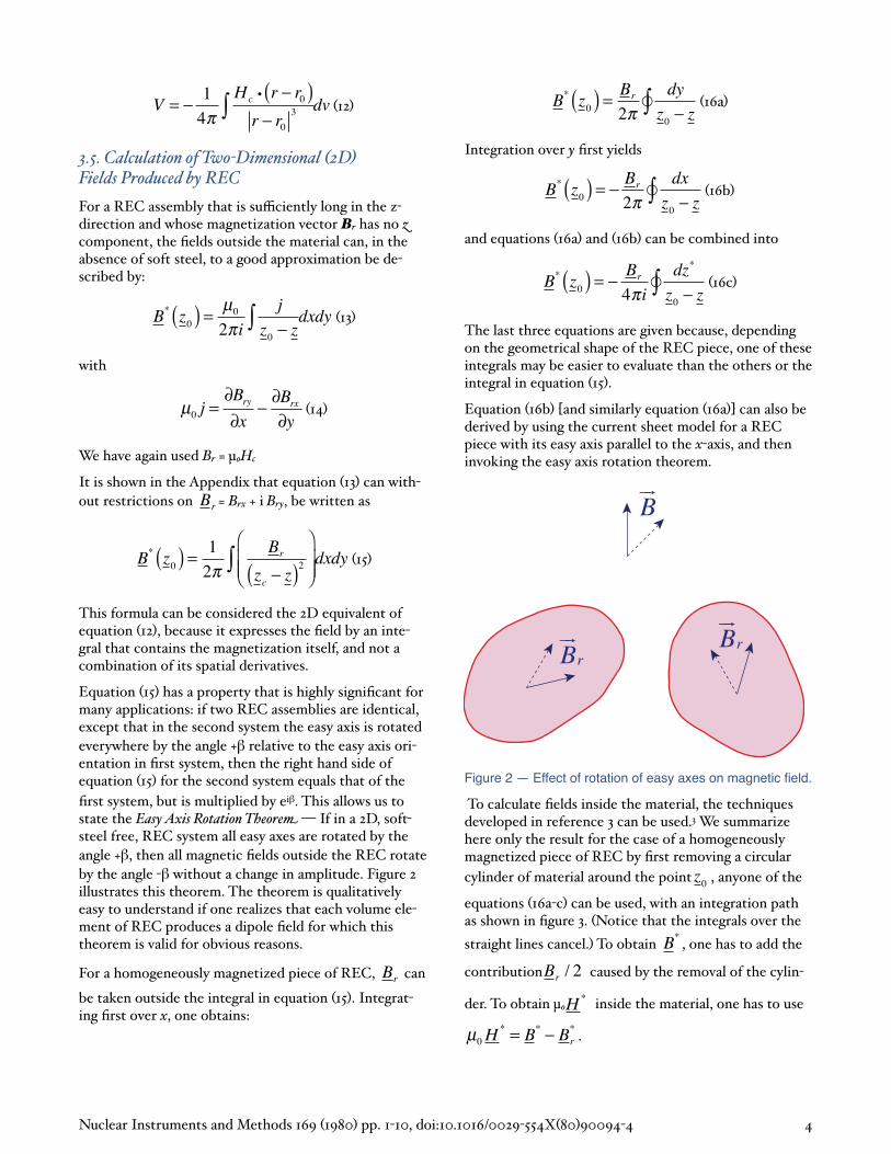
To calculate fields inside the material, the techniques developed in reference 3 can be used.3 We summarize here only the result for the case of a homogeneously magnetized piece of REC by first removing a circular

cylinder of material around the pointz0 , anyone of the

equations 16a c can be used, with an integration path as shown in figure 3. Notice that the integrals over the

straight lines cancel. To obtain B* , one has to add the

contributionBr / 2 caused by the removal of the cylin

der. To obtain μoH * inside the material, one has to use

μ0H*= B* Br

*.

Nuclear Instruments and Methods 169 1980 pp. 1 10, doi:10.1016/0029 554X 80 90094 4 4

Even though it is possible to write down explicitly the fields produced by the multipole magnets discussed below, it is more convenient, and gives more insight, to use the Taylor expansions introduced in equations 4a, b . To obtain the expansion coe cients, one has to use in equations 16a c .

1

z0 z=

z0n 1

znn=1

17a

and for use in equation 15 , one obtains by di erentiation of equation 17a :

1

z0 z( )2 =

nz0n 1

zn+1n=1

18a

For a field expansion radially outside the magnet, one has to use

1

z0 z=

z0n 1

znn=1

17b

and

1

z0 z( )2 =

nz0n 1

zn+1n=1

18b

4. REC Multipole Magnets 4.1. Multipoles with Continuous Easy Axis Orientatio

To produce a strong 2N multipole magnet with good field quality, one wants to arrange the REC in such a way

that in equation 4b , bn is large, and that all other bnare as small as possible. Using equation 18a in equation 15 , we obtain

bn =n

2

Br

zn+1da 19b

With Br = Brei ( ), andz = rei , we get

bn =n

2

Br exp i ( ) n +1( ){ }rn+1

rdrd 19

From this equation follows directly that the largest possible real bn is obtained by choosing

( ) = N +1( ) 20

Equation 19 also shows the expected fact that a piece of REC contributes the more to the multipole strength

the closer it is to the point z = 0.

Figure 3 — Integration path for calculation of field inside the REC material

If the space between the two circles z = r1 and z = r2 is

filled. with REC, with Br a constant and φ given by

equation 20 , bn = 0 for N, giving for

B* z0( ) =z0

r1

N 1

BrN

N 11

r1r2

N 1

; for N 2

21a

B* z0( ) = Br lnr1r2

; for N = 1 21b

Inspection of the field for z > r2, using equation 18b

instead of equation 18a , shows that the field outside this multi pole magnet is exactly zero.

The fact that “recipe” equation 20 leads to a perfect multipole is not surprising when one realizes that as a direct consequence of equation 20 , the current density j in equation 8b inside the material has only the component jc = Hc N + 1 sin Nφ/r, with the current

sheets at the inside and outside boundaries of the REC also being proportional to sin Nφ.

Equations 21 were given for N = 1, 2 by Blewett4 in an unpublished report in 1965. However that report does not mention the anisotropy of the material, and consequently does not give the design recipe represented by equation 20 .

Nuclear Instruments and Methods 169 1980 pp. 1 10, doi:10.1016/0029 554X 80 90094 4 5

The multipole just discussed obviously produces the strongest and cleanest multi pole field possible within a circular aperture of a pure REC multi pole with a given amount of material. A study of the field inside the material shows that one can find closed curves that are perpendicular to H everywhere. Replacing the material inside such a closed curve by soft steel with very large permeability will reduce the amount of REC without significantly changing the field in the aperture. It is my subjective judgement that the potential savings are too small to be worth the resulting complication of construction in the case of strong multipoles, and this avenue has therefore not been pursued in the study of the segmented multipoles.

Since the above mentioned steel contours can range into the aperture region, this approach can be used to design multipoles that have steel poles controlling the field in the aperture and use fairly little REC. However, with the exception of dipoles, those magnets have weaker pole tip fields than the pure REC multi poles. While it is my opinion that incorporation of steel into the design will not increase the upper limit of the achievable multi pole strength, given by equation 21a , I have no proof for this assessment.

In order to satisfy equation 20 , we require strong magnetic fields during the alignment process with a distribution of local direction given by equation 20 . Since a 2D vacuum field satisfying that condition must behave like

B* ~ 1 / N+1 in the region of interest, it is highly unlikely

that one can produce REC with precisely the desired easy axis distribution, particularly for small magnets. Fortunately, the segmented magnet design discussed below has a performance very close to that of the ideal REC multipole.

4.2. The Segmented Multipole Magne

To get a reasonable approximation to equation 20 , we segment the magnet into M geometrically identical pieces such that, ignoring the direction of the easy axes, the structure is invariant to rotation by the angle 2 /M

about z = 0 . Throughout each piece, the easy axis

points in the same direction, but that direction advances in the x y coordinate system by N+1 2 /M from one

piece to the next. This means that relative to a coordinate system fixed in the piece, the easy axis advances by N2 /M from one piece to the next.

Using equations 17 , 16c and 4b , bn produced by one

such piece can be expressed for both positive and negative by

bn = sgn n( )Br

4 i

dz*

zn22

If the contribution to bn coming from a reference piece

isCn , then the contribution from a piece rotated by

relative to the reference piece is Cneix N+1( )e ix n+1( ) ,

where the first exponential factor comes from the rotation of the easy axis by N+1 , and the second factor from the integral in equation 22 . With = 2 /M, we get for the whole assembly

bn = Cn expi2 m N n( )

Mm=0

N 1

22b

If N /M is zero or a positive or negative integer, the sum equals M. If N /M is not an integer, the geometrical series is zero, yielding

B* z0( ) = M Cnv

z0n 1; n = N + vM 23

Depending whether one wants to know the fields in the aperture region or outside the magnet, one takes the sum over either positive or negative .

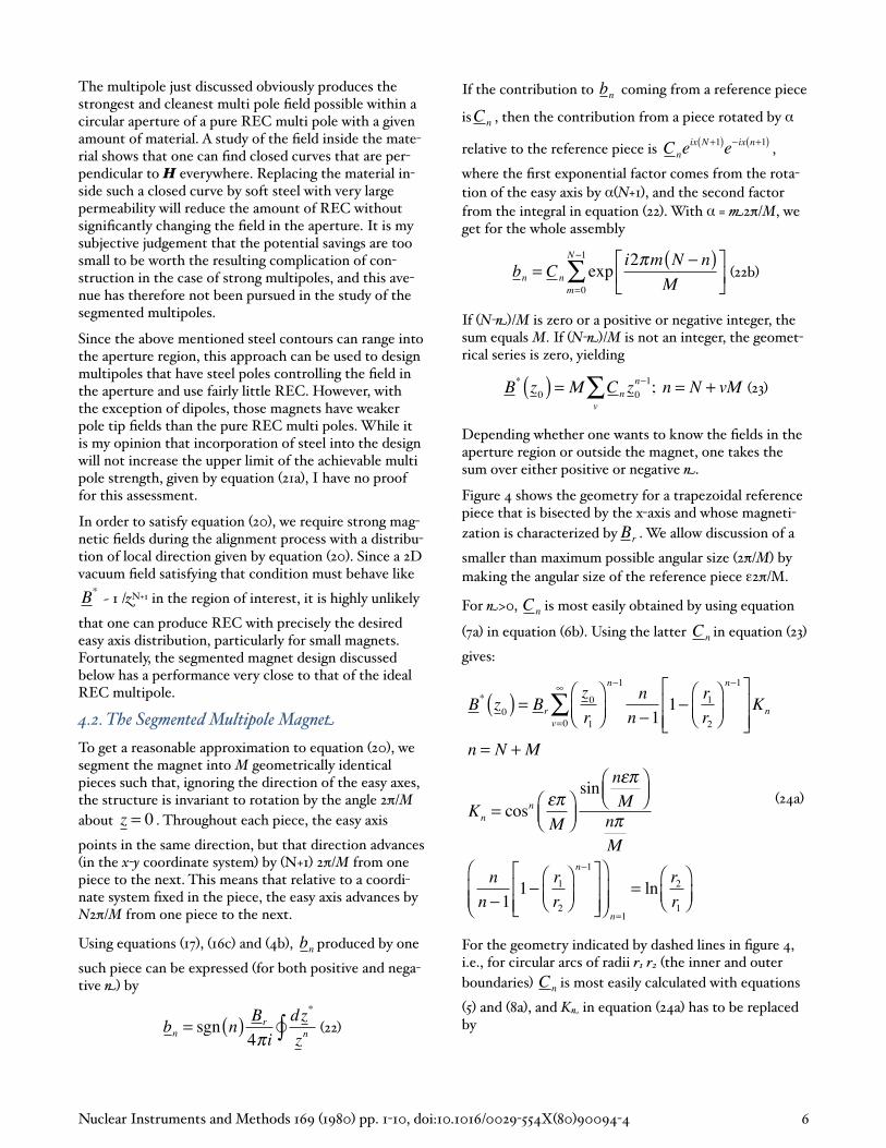
Figure 4 shows the geometry for a trapezoidal reference piece that is bisected by the x axis and whose magneti

zation is characterized by Br . We allow discussion of a

smaller than maximum possible angular size 2 /M by making the angular size of the reference piece 2 /M.

For >0, Cn is most easily obtained by using equation

7a in equation 6b . Using the latter Cn in equation 23

gives:

B* z0( ) = Br

z0r1v=0

n 1n

n 11

r1r2

n 1

Kn

n = N +M

Kn = cosn

M

sinn

Mn

M

n

n 11

r1r2

n 1

n=1

= lnr2r1

24a

For the geometry indicated by dashed lines in figure 4, i.e., for circular arcs of radii r1 r2 the inner and outer

boundaries Cn is most easily calculated with equations

5 and 8a , and K in equation 24a has to be replaced by

Nuclear Instruments and Methods 169 1980 pp. 1 10, doi:10.1016/0029 554X 80 90094 4 6

Kn =

sinn +1( )M

n +1( )M

24b

It follows from equation 24 that for a given Br and for = N > 1, there always exists an upper limit for the field

strength at the magnet aperture, while for the dipole this upper limit is controlled in essence by the B H curve in the third quadrant.

�M

��M

X

Figure 4 — One piece of a segmented REC multipole.

Comparison of equations 24 with equations 21 shows that the fundamental harmonic of the segmented multipole is smaller by a factor KN than the equivalent ideal REC multipole and that for = 1 one comes close to the ideal strength if the number of REC pieces per period.

M '=M

N25

is equal to or larger than eight.

In the somewhat unusual case that one elects to use a small value like 2 for M’, it follows in general from equations 5 and 8a and specifically, of course, from equations 24a, b that KN is largest not when equals one, but for

=M

2 N +1( )=

M '

2 1+ N 1( )26

provided this value is smaller than one.

From equations 24a, b we can extract the amplitude of the field due to the harmonic = N+ M relative to the amplitude of the fundamental N. For the qualitatively representative case of trapezoidal REC pieces, we ob

tain from equation 24a for that ratio Q at z = r,

and for = 1

Q v( ) =r

r1

vMN 1

n 1cosvM

M

1 r1 / r2( )n 1

1 r1 / r2( )N 1 27

For r = r1, the values for Q are uncomfortably large. Fortunately in most applications the largest r/r1 of concern is, while close to one, still small enough so that the factor r/r1 vM reduces Q to acceptable levels even for the most unfavorable case, = 1. Should, however, Q 1 be larger than acceptable, Q 1 can be made to vanish by choosing

=1

1+ N /M( )= 1

1

1+M '( )28

For that value of , Q becomes

Q v( ) =r

r1

vMN 1

n 1cosvM

M

x sinv 1

1+M ' / sin1+M '

x 1r1r2

n 1

/1r1r2

N 1

29

For reasonably large values of M, it is unlikely that the worst of these harmonics = N + 2M will ever cause any problems.

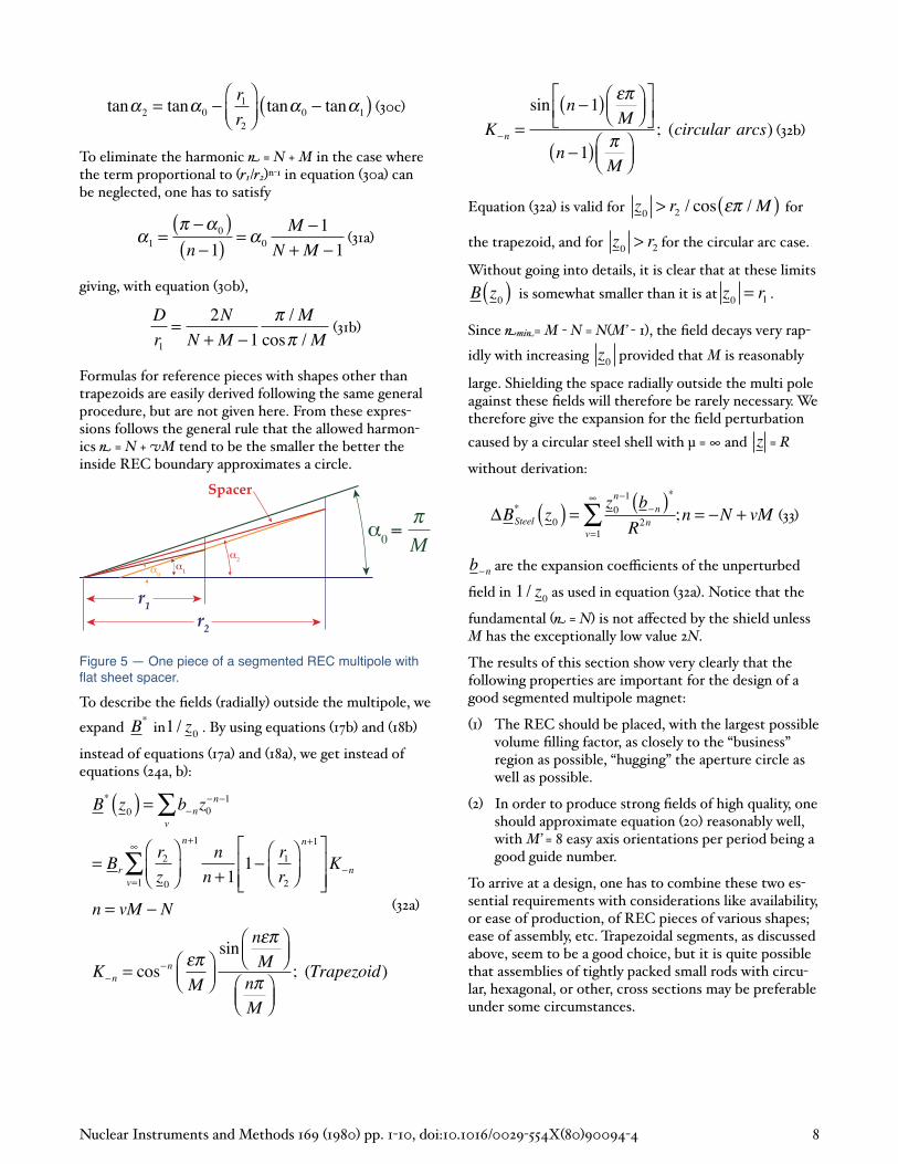
The design represented by equation 28 means that one has a wedge shaped non magnetic space between adjacent pieces of REC. While these gaps could be implemented by having appropriate notches in the magnet assembly fixture, an alternate method of making Q 1 = 0 would be the use of a non magnetic spacer between adjacent REC pieces. For that kind of design it would be advantageous to have spacers of uniform thickness D. Referring to figure 5 for the definition of the symbols, application of equation 16a and 17a gives for the field in that case

B* z0( ) = Br

z0r1r=0

n 1cos 0 cos

n 11

n 1( ) 0

x sin 0 + 1 n 1( )r2 cos 2

r2 cos 1

n 1

sin 0 + 2 n 1( )

30a

with

D

r1= 2cos 0 tan 0 tan 1( )

2 0 1( )cos 0

30b

Nuclear Instruments and Methods 169 1980 pp. 1 10, doi:10.1016/0029 554X 80 90094 4 7

tan 2 = tan 0

r1r2

tan 0 tan 1( ) 30c

To eliminate the harmonic = N + M in the case where the term proportional to r1/r2 n 1 in equation 30a can be neglected, one has to satisfy

1 =0( )

n 1( )= 0

M 1

N +M 131a

giving, with equation 30b ,

D

r1=

2N

N +M 1

/M

cos /M31b

Formulas for reference pieces with shapes other than trapezoids are easily derived following the same general procedure, but are not given here. From these expressions follows the general rule that the allowed harmonics = N + M tend to be the smaller the better the inside REC boundary approximates a circle.

01

2

�M0

=

r1r2

Spacer

Figure 5 — One piece of a segmented REC multipole with flat sheet spacer.

To describe the fields radially outside the multipole, we

expand B* in1 / z0 . By using equations 17b and 18b

instead of equations 17a and 18a , we get instead of equations 24a, b :

B* z0( ) = b nv

z0n 1

= Br

r2z0v=1

n+1n

n +11

r1r2

n+1

K n

n = vM N

K n = cos n

M

sinn

Mn

M

; (Trapezoid)

32a

K n =

sin n 1( )M

n 1( )M

; (circular arcs) 32b

Equation 32a is valid for z0 > r2 / cos /M( ) for

the trapezoid, and for z0 > r2 for the circular arc case.

Without going into details, it is clear that at these limits

B z0( ) is somewhat smaller than it is at z0 = r1 .

Since mi = M N = N M’ 1 , the field decays very rap

idly with increasing z0 provided that M is reasonably

large. Shielding the space radially outside the multi pole against these fields will therefore be rarely necessary. We therefore give the expansion for the field perturbation

caused by a circular steel shell with μ = and z = R

without derivation:

BSteel* z0( ) =

z0n 1 b n( )

*

R2nv=1

;n = N + vM 33

b n are the expansion coe cients of the unperturbed

field in 1 / z0 as used in equation 32a . Notice that the

fundamental = N is not a ected by the shield unless M has the exceptionally low value 2N.

The results of this section show very clearly that the following properties are important for the design of a good segmented multipole magnet:

1 The REC should be placed, with the largest possible volume filling factor, as closely to the “business” region as possible, “hugging” the aperture circle as well as possible.

2 In order to produce strong fields of high quality, one should approximate equation 20 reasonably well, with M’ = 8 easy axis orientations per period being a good guide number.

To arrive at a design, one has to combine these two essential requirements with considerations like availability, or ease of production, of REC pieces of various shapes; ease of assembly, etc. Trapezoidal segments, as discussed above, seem to be a good choice, but it is quite possible that assemblies of tightly packed small rods with circular, hexagonal, or other, cross sections may be preferable under some circumstances.

Nuclear Instruments and Methods 169 1980 pp. 1 10, doi:10.1016/0029 554X 80 90094 4 8

4.3. The Segmented REC Quadrupol

Because of their special importance for accelerators, we discuss some details of quadrupoles, adding to the summaries published elsewhere 5,6 Since quadrupoles with trapezoidal segments are quite typical, we restrict the discussion to this specific class of magnets.

From equation 24a follows for the fundamental har

monic for = 1:

B* z0( ) =z0r1Br2 1

r1r2

K2

K2 = cos2

M

sin 2 /M( )2 /M

34

Table 1 shows that in order to get a strong quadrupole, one should choose M = 12 or 16. The gradients achievable with a 16 piece quadrupole are impressive, particularly when they are compared with those of conventional quadrupoles. For M = 16, r2/r1 = 4, which is still quite compact and Br = 0.95 T which is commercially available , one obtains an aperture field of 1.34 T. In contrast, a high quality conventional quadrupole is very di cult to make with more than 1 T at the aperture, and even that is possible only for fairly large aperture magnets. High aperture fields are of particular importance for linear accelerators with small apertures. For an aperture with r1 = 2 mm, it it possible to achieve a gradient B’ = 6 T cm 1, and the diameter of such a quadrupole could be smaller than 2 cm. Clearly, it is impossible to achieve anything resembling this with conventional magnets and conventional REC quadrupole designs fall short of this gradient by at least a factor of 2.

M 4 8 12 16 20 24

K2 0.32 0.77 0.89 0.94 0.96 0.97

Figure 6 shows a schematic cross section of a 16 piece quadrupole, with the easy axis direction indicated in each piece. It follows from that diagram that one needs pieces with five di erent orientations of the easy axis relative to the trapezoidal shape to make this 16 piece quadrupole.

x

y

Figure 6 — Schematic cross section of a 16-piece REC quadrupole.

If one rotates all easy axes by 22.5° in the same direction, only four di erent pieces are required, which may be advantageous for the manufacturer. Since one has, in either case, a reasonably large number of pieces that are supposed to be identical, it may be advantageous to measure magnetization direction and magnitude for each piece, and then assemble the quadrupole in such a way that magnetization errors do the least harm to the field quality. For this reason, it may be a blessing in disguise that with present manufacturing techniques, the individual REC pieces are fairly small. This often forces the use of several layers of REC in the axial direction, increasing the number of pieces and therefore improving the error canceling statistics.

For a 16 piece quadrupole with r1/r2 = 0.25, the first un

desirable harmonic = 18 field has, at z = r1, an ampli

tude that is approximately 6 of the fundamental see equation 27 for N = 2 . Eliminating that harmonic with a flat sheet of the thickness given by equation 31b , the first non vanishing harmonic is = 34, with a relative amplitude of about 3 at the full aperture. The order of this harmonic is high enough that no attempt has yet been made to also eliminate it.

The fringe fields at the end of a segmented, quadrupole or other multipole are fairly easily calculated by using

the charge sheet model and equation 11 . If the cross sections of the REC pieces are trapezoidal, the charge sheets have rectangular cross sections and the integrals can be expressed by elementary transcendental functions, making the 3D field calculation rather easy. The relevant formulas are not reproduced here because the

Nuclear Instruments and Methods 169 1980 pp. 1 10, doi:10.1016/0029 554X 80 90094 4 9

fringe fields of REC multipole magnets have some rather remarkable properties to be discussed in section I 4.4 that make fringe field calculations necessary in only very rare instances.

Holsinger has built a prototype quadrupole with r1 = 1.1 cm; r2 = 3 cm; M = 16; and consisting of three 16 piece layers in the axial direction. Comparisons were made between measurements of that magnet, computer runs of that magnet with PANDIRA,7 and the predictions made with the simple theory presented here. The results obtained with these procedures agreed very well with regard to the amplitude of the quadrupole field and the allowed higher harmonic = 18. The only significant, but expected, discrepancy was the presence of the harmonics = 6, 10, 14 in the computer model and the real magnet, while these harmonics do not exist in the sim

ple model that assumes μ = μ = 1. At z = r1 the ampli

tudes of these harmonics were, relative to the quadrupole field, 0.2 for = 6; 0.1 for = 14; and <<0.1 for = 10. While these errors are so small that they are unlikely to cause problems in most applications, one can easily imagine methods to eliminate these harmonics, if necessary. If, for instance, one has a gap between adjacent pieces for the elimination of = 18, one would incorporate movable thin strips of soft steel into these gaps to tune away these undesired harmonics. The real magnet also had an approximately 0.5 sextupole, as well as some other multi poles, present. Since the individual REC pieces were not measured, it is expected that these harmonics can be significantly reduced when this is done and properly taken into account in the assembly. Another obvious tuning method would be the removal or addition of small amounts of REC at appropriate locations, but it is unlikely that such e orts will really be necessary.

4.4 Important Practical Consequences of Applicability of Linear Superposition Principl

It is obvious that the linear superposition principle is of crucial importance not only for specific important theorems, like the easy axis rotation theorem or the selection rule for possible harmonics equation 24a , but to the whole mathematical description of REC magnets presented here. However, there are some very important practical consequences of the linear superposition principle that are obtainable without any mathematical derivations.

We consider first the following combination of two REC multipole magnets: one quadrupole is located, tightly fitting, inside the aperture region of another quadrupole. If each of these quadrupoles alone produces the same gradient, and both quadrupoles are rotated about the common axis by equal amounts in opposite directions, then the gradient in the aperture can be con

tinuously changed between zero and twice the strength of the individual quadrupole. By similarly pairing of two dissimilar multipoles, one can make combined function mag nets.

Care has to be taken for these combinations of REC magnets, and in particular for combinations of conventional steel magnets with REC magnets, that the REC is not driven into the nonlinear part of the B H curve. A combination of magnets that would be fairly immune from this danger is a multipole inside the homogeneous field of a coaxial solenoid, since in this case the solenoidal field is everywhere perpendicular to the easy axis.

A di erent method to modify the e ective strength of a REC quadrupole would be to assemble it from quadrupoles of relatively short axial lengths whose quadrupole field orientations can be adjusted. While this would be fairly easy to do, such a scheme obviously modifies the optical properties of the system in a non trivial way, and this aspect of such a system is currently under investigation .8

Another important application of the superposition principle is the treatment of the fringe fields at the ends of multi pole magnets. We deal here with two distinctly di erent aspects of fringe fields that are both very simple and important.

First we consider a multipole of finite physical length L whose left end is cut o in an arbitrary fashion, and whose right end is shaped such that the left end would fit it perfectly, without forming any gap. See figure 7 . Another way to express that geometry is to state that the length of REC along any line parallel to the axis is either L or zero. Keeping the left end of the multipole fixed in space, we first consider the field quantity G1 r, φ, produced by a semi infinite multipole, with Go r, φ

representing the 20 field deep inside where it does not depend on .

Figure 7 — Geometry of specific finite length REC multipole

Then the field quantity G r, φ, produced by a multi

pole of length L is given by

G r, , z( ) = G1 r, , z( ) G1 r, , z L( ) 35

Nuclear Instruments and Methods 169 1980 pp. 1 10, doi:10.1016/0029 554X 80 90094 4 10

If we now calculate the optically important

G z( )dz 35b

it is easy to see that equation 35 leads to

G r, , z( )dz = LG0 r,( ) 36

This equation says not only that the e ective length for the fundamental harmonic of interest equals the physical length of the multi pole, but also that the integral over a field quantity vanishes if that field quantity is zero in the 2D cross section!

Next, we consider the properties of the fringe fields produced by a semi infinite multipole, produced by cutting an infinite multipole by the x y plane at z = 0 see figure 8 , i.e., we look at the fringe field function G1 for the specific case of the “square” end. If V1 r, φ, is

the scalar potential produced by the multipole located at >0, then the scalar potential produced by the multipole

located at <0 must be V1 r, φ, . If Vo r, φ is the scalar

potential inside the infinitely long multipole, the following obviously must hold:

V1 r, , z( ) +V1 r, , z( ) =V0 r,( ) 37

Applying the appropriate operator to this equation to get the field quantity G1 r, φ, of interest, we get, if no

derivative with respect to is involved:

G1 r, , z( ) +G1 r, , z( ) = G0 r,( ) = 2G1 r, ,0( )

38

From this it follows that

G1 r, , z( )dz =z1

z1G0 r,( ) 39

if 1 is su ciently large. This means that the e ective boundary is at = 0, and that the fringe field integral over a field quantity vanishes if that quantity is zero in the 2D cross section. Notice that this statement is stronger than the one made above with respect to equation 36 that required integration over the fringe fields of both ends.

0 z

Figure 8 — Fields at the end of a REC multipole

If the operator to obtain the field quantity of interest is proportional to / z , we get instead of equation 38

G1 r, , z( ) = 1( )mG1 r, , z( ) 40

Integrating this G1 r, φ, over the fringe field region

gives zero when 2, but not necessarily when = 1.

Appendix Using equations 14 in equation 13 , one of the two integrals that have to be evaluated in equation 13 is

I1 =1

2 i

Hcy / X

z0 x iydxdy 41

Carrying out the integration over x first, and integrating by parts, one obtains

I1 =1

2 i

Hcy

z0 zdy

1

2 i

Hcy

z0 z( )2dxdy 42

Included in the integration area is a thin strip of vacuum outside the REC. Hcy = 0 there, so that the line integral over y vanishes. Applying the same technique to the other integral necessary for the evaluation of the integral in equation 13 , one obtains equation 15 .

I would like to thank J. A. Farrell, T. D. Hayward, E. A. Knapp Los Alamos Scientific Laboratory and Robert L. Gluckstern University of Maryland for their active interest, support and discussions of this work. Karl Strnat very kindly proofread the section dealing with the material production and properties.

Massoud Kaviany Lawrence Berkeley Laboratory made some useful computer runs and Ron Holsinger shared the results of his computer runs and practical experiences and contributed greatly with several useful suggestions and many stimulating discussions.

Nuclear Instruments and Methods 169 1980 pp. 1 10, doi:10.1016/0029 554X 80 90094 4 11

Publishing HistoryReceived 20 August 1979, first published 1980. Reformatted and color illustrations added by Mark Duncan in June 2009.

This work was supported by the Los Alamos Scientific Laboratory and the Lawrence Berkeley Laboratory of the US Department of Energy under contract No. W7405 ENG 48.

References

Nuclear Instruments and Methods 169 1980 pp. 1 10, doi:10.1016/0029 554X 80 90094 4 12

1 Karl J. Strnat and G. I. Ho er; Technical Report, AFML TR 65 446, Wright Paterson Air Force Base, 1966 ; J. B. Y. Tsui, D. J. Iden, K. J. Strnat and A. J.

Evers; IEEE Transactions Magnetics 2 1972 p. 188.

2 Malcolm McCaig, Permanent Magnets in Theory and Practice, John Wiley, London, 1977 .

3 Klaus Halbach; Nuclear Instruments and Methods 78 1970 185.

4 J. P. Blewett; BNL Internal Report, AADD 89 1965 .

5 Klaus Halbach, “Strong Rare Earth Cobalt Quadrupoles,” Proceedings 1979 Particle Accelerator Conference, IEEE Transactions Nuclear Science NS 26, issue 3, Part 2, 1979 pp. 3882 3884; doi: 10.1109/TNS.1979.4330638

6 Ron F. Holsinger and Klaus Halbach; Proceedings 4th International Workshop on Rare Earth Cobalt Permanent Magnets 1979 p. 37.

7 Ron F. Holsinger and Klaus Halbach; to be published.

8 Robert L. Gluckstern; private communication.