64
Perspectives of tearing modes control in RFX-mod Paolo Zanca Consorzio RFX, Associazione Euratom-ENEA sulla Fusione, Padova, Italy
| Date post: | 27-Dec-2015 |
| Category: |
Documents |
| Upload: | augustine-mccormick |
| View: | 224 times |
| Download: | 3 times |

Perspectives of
tearing
modes control in RFX-mod
Paolo Zanca
Consorzio RFX, Associazione Euratom-ENEA sulla Fusione, Padova, Italy

RFX-mod contributions to TMs control (I)
• Demonstrated the possibility of the feedback control onto TMs
• Clean-Mode-Control (CMC) based on the de-aliasing of the measurements from the coils produced sidebands

RFX-mod contributions to TMs control (I)
• Demonstrated the possibility of the feedback control onto TMs
• Clean-Mode-Control (CMC) based on the de-aliasing of the measurements from the coils produced sidebands
• Not obvious results: phase-flip instability?

RFX-mod contributions to TMs control (I)
• Demonstrated the possibility of the feedback control onto TMs
• Clean-Mode-Control (CMC) based on the de-aliasing of the measurements from the coils produced sidebands
• Not obvious results: phase-flip instability?
• No-sign of phase-flip instability; equilibrium condition can be established where CMC induces quasi-uniform rotations of TMs

• Wall-unlocking of TMs with CMC
• In general, the feedback cannot suppress the non-linear tearing modes requested by the dynamo.
• The feedback keeps at low amplitude the TMs edge radial field
• Improvement of the magnetic structure: sawtooth of the m=1 n=-7 which produces transient QSH configurations
RFX-mod contributions to TMs control (II)

• Increase the QSH duration → recipes under investigation
• Which are the possibilities to reduce further the TMs edge radial field? → Model required
CMC optimizations
RFXlocking
• Semi-analitical approach in cylindrical geometry
• Newcomb’s equation for global TMs profiles
• Resonant surface amplitudes imposed from experiments estimates
• Viscous and electromagnetic torques for phase evolution
• Radial field diffusion across the shell(s)
• Feedback equations for the coils current
• It describes fairly well the RFX-mod phenomenology →L.Piron talk

General analysis of the TM control

plasma
Sensors CoilsVessel
Single-shell external coils

Normalized edge radial field
•The feedaback action keeps low the normalized edge radial field
)()(ˆ,
,,,nm
nmrsens
nmr
nmsens rbrbb
• At best b^sens can be made close but not smaller than the
ideal-shell limit

plasma
Sensors CoilsVessel
Feedback limit

plasma
Sensors CoilsVessel
Feedback limit

plasma
Sensors
br=0 everywhere: impossible
CoilsVessel
Feedback limit

Role of the Vessel
• The stabilizing effect of the vessel is crucial for having low b^
sens and moderate power request to the coils
• The shorter τw the faster must be the control system (fc=1/Δt) to avoid feedback (high-gain) induced instabilities
• Optimum range: τw >10ms better τw 100ms
plasma
Sensors Coils Vessel
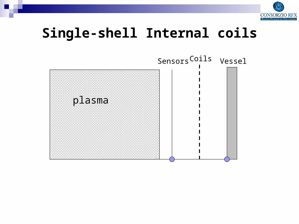
Single-shell Internal coils

plasma
Sensors Coils Vessel
Single-shell Internal coils

Single-shell Internal coils
• Continuous-time feedback → solution ωω0 with br(rsens) 0 for large gains
•Discrete-time feedback : including the latency Δt the high-gain instability may occur
• The good control region is not accessible for realistic TM amplitudes.
• For stable gains b^sens is determined by the ideal-shell limit,
which is large due to the loose-fitting vessel required by the coils dimension

RFP design for good TM control
(a personal view)

Premise
• The passive stabilization provided by a thick shell does not solve the wall-locking problem
• In the thick-shell regime wall-locking threshold ~σ1/4
• Feedback is mandatory to keep TMs rotating
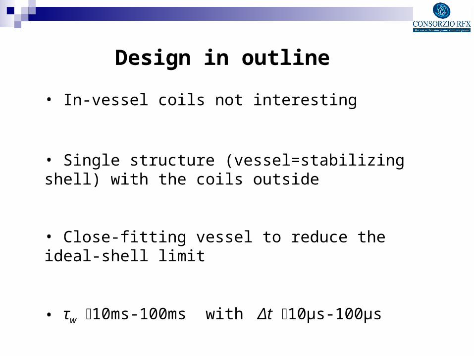
Design in outline • In-vessel coils not interesting
• Single structure (vessel=stabilizing shell) with the coils outside
• Close-fitting vessel to reduce the ideal-shell limit
• τw 10ms-100ms with Δt 10μs-100μs

RFX-mod perspectives (a personal view)

RFX-mod layout
• 3ms vacuum-vessel, 100ms copper shell, ~25ms mechanical structures supporting the coils
• The control limit is mainly provided by the 100ms copper shell

RFX-mod status
0
0,2
0,4
0,6
0,8
1
8 10 12 14 16
b^
a ideal shell
b^
a RFXlocking
b^
a experiment
-n
Gain optimization guided by RFXlocking simulations for the RFX-mod case
m=1 TMs

Optimizations
• Get closer to the ideal-shell limit (minor optimization)
• Reduce the ideal-shell limit by hardware modifications (major optimization)

Minor optimizations
• Increase the coils amplifiers bandwidth: maximum current and rensponse time
• Acquisition of the derivative signal dbr /dt in order to have a better implementation of the derivative control (to compensate the delay of the coils amplifiers)
• Compensation of the toroidal effects by static decoupler between coils and sensors only partially exploited
• Compensation of the shell non-homogeneities requires dynamic decoupler (work in progress)

Major optimization
• Approach the shell to the plasma edge possibly simplifying the boundary (removing the present vacuum vessel which is 3cm thick)
• Moving the τw =100ms shell from b=0.5125m to b=0.475m (a=0.459) a factor 3 reduction of the edge radial field is predicted by RFXlocking

Conclusions• CMC keeps TMs into rotation
• Edge radial field: ideal-shell limit found both with the in-vessel and out-vessel coils → br(a)=0 cannot be realized
• The vessel=shell must be placed close the plasma → coils outside the vessel. Is a close-fitting vessel implementable in a reactor?
• The feedback helps the vessel to behave close to an ideal shell → τw cannot be too short

spare

Edge radial field control by feedback
0
5
10
15
0 0,02 0,04 0,06 0,08 0,1
w=100ms
rwi
=0.475m rf=r
wi
rwi
=0.5125m rf=r
wi
RFX-mod experiment
max
[1(
)] (
mm
)
time(s)
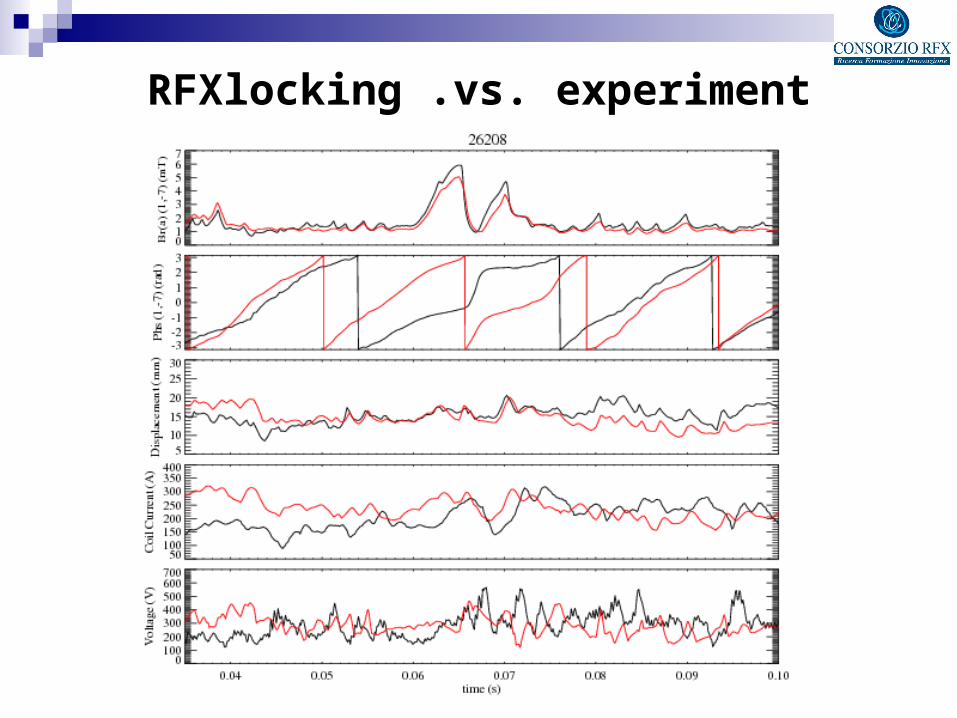
RFXlocking .vs. experiment

0
20
40
60
0
0,05
0,1
0,02 0,04 0,06 0,08 0,1
m=1, n=-7
brs
b^
a
mT
time(s)
Normalized edge radial field: weak brs dependence
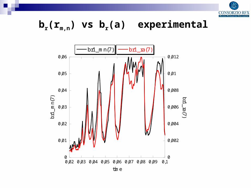
br(rm,n) vs br(a) experimental
0
0,01
0,02
0,03
0,04
0,05
0,06
0
0,002
0,004
0,006
0,008
0,01
0,012
0,02 0,03 0,04 0,05 0,06 0,07 0,08 0,09 0,1
br1_mn(7) br1_ra(7)br
1_m
n(7)
br1_ra(7)
time

Locking threshold
The present analysis valid for w<<rw cannot be extrapolated to very long w
2
6
10
1 10 100
Wall-locking threshold m=1, n=-7 (mT)
w (ms)
300

0,22
0,23
0,24
0,25
0,26
0,27
0,28
0,29
0 0.5 1 1.5 2 2.5 3
m=1 n=-8
b^
a
c(ms)
Edge radial field .vs. current time constant

a = 0.459m
rw i = 0.475m
c = 0.5815m
Single mode simulations: external coils
0,1
1
10-4 10-3 0,01 0,1 1
rf=a
1.1252.253672
b^
f
d/
w
ideal shell0.03
-Kpxa/(0.96 )=
0,04
0,06
0,08
0,1
0,3
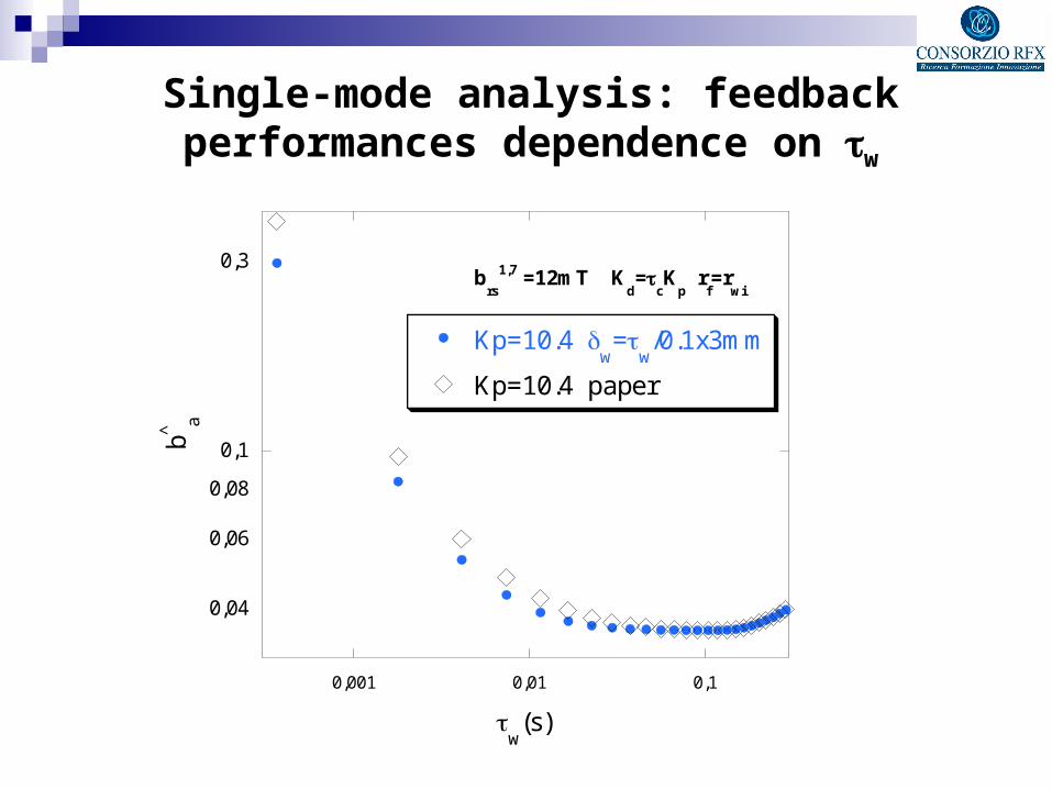
0,001 0,01 0,1
Kp=10.4 w=
w/0.1x3mm
Kp=10.4 paper
b^ a
w(s)
brs
1,7 =12mT Kd=
cK
p r
f=r
wi
Single-mode analysis: feedback performances dependence on w

1000
104
105
106
107
0,001 0,01 0,1
Kp=10.4 w=
w/0.1x3mm
Kp=10.4 paper
abs(
IcV
c) (
W)
w(s)
brs
1,7 =12mT Kd=
cK
p r
f=r
wi
Single-mode analysis: feedback performances dependence on w

1000
104
105
106
107
0,05 0,052 0,054 0,056 0,058 0,06
rf=r
w
w=0.1s;
d=0.1ms
rf=a
w=0.1s;
d=0.1ms
rf=a
w=0.01s;
d=0.01ms
max
i,j(P
i,j)(
W)
time(s)
Multi-mode analysis: power dependence on w

Edge radial field: w dependence
Data averaged on 0.1s simulation
0,04
0,06
0,080,1
0,3
8 10 12 14 16 18
rf=r
wi
ideal shell
w=100ms
w=3ms
w=10ms
w=200ms
b^ a
-n
m=1
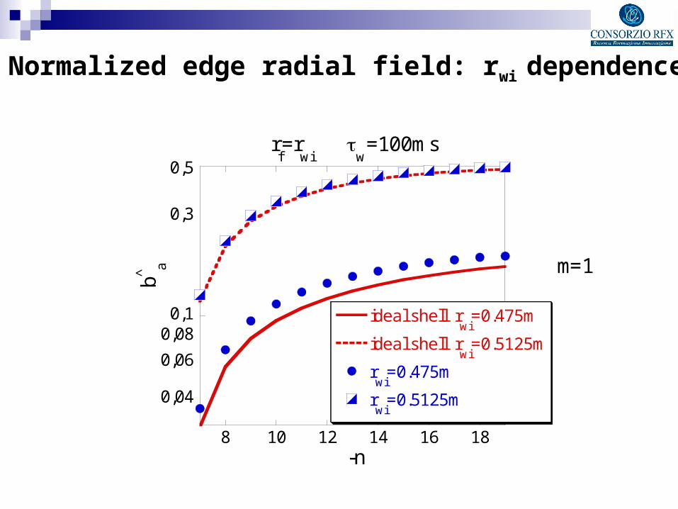
Normalized edge radial field: rwi dependence
0,04
0,06
0,080,1
0,3
0,5
8 10 12 14 16 18
rf=r
wi
w=100ms
ideal shell rwi
=0.475m
ideal shell rwi
=0.5125m
rwi
=0.475m
rwi
=0.5125m
b^ a
-n
m=1

Normalized edge radial field: no rf dependence
0,04
0,06
0,080,1
0,3
8 10 12 14 16 18
w=100ms
ideal shellrf=r
wi=0.475m
rf=a=0.459m
b^ a
-n
m=1

0
0.5
1
1.5
2
0,05 0,055 0,06 0,065
maxi,j(br
i,j) clean
maxi,j(br
i,j) raw
mT
time(s)
Out-vessel coils: signals
4x48 both for coils (c = 0.5815m) and sensors (rwi = 0.475m )

Single-shell: discrete feedback
ttt jj 1 Δt = latency of the system
;1,,
1,,
1,
jnm
rnm
djnm
rnm
pjjnm
c tbdt
dKtbKttV

External coils: discrete feedback τw=100ms
0,03
0,04
0,05
0,06
0,1
0,2
2 6 10 14
w=100mscontinuous
t=10-6
t=10-5
t=10-4
t=10-3
< b
^ f >
-Kp rwi
/(0.96)
a)
ideal-shell limit
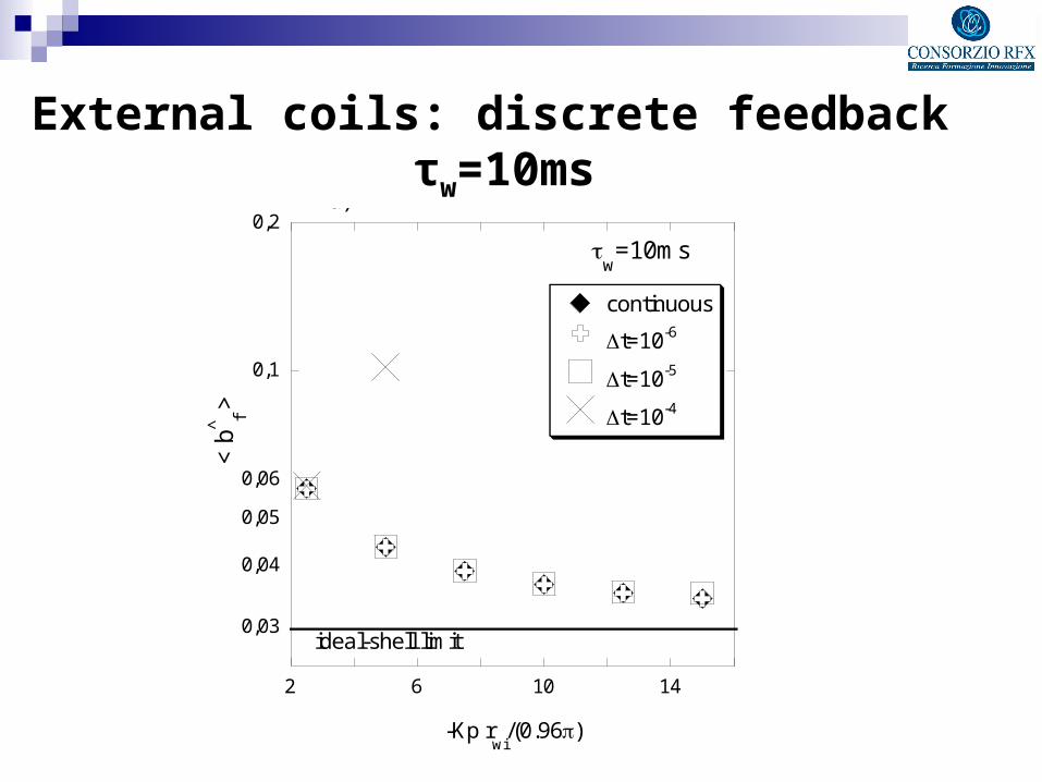
External coils: discrete feedback τw=10ms
0,03
0,04
0,05
0,06
0,1
0,2
2 6 10 14
w=10ms
continuous
t=10-6
t=10-5
t=10-4
< b
^ f >
-Kp rwi
/(0.96)
a)
ideal-shell limit

External coils: discrete feedback τw=1ms
0,03
0,04
0,05
0,06
0,1
0,2
2 6 10 14
w=1ms
continuous
t=10-6
t=10-5
< b
^ f >
-Kp rwi
/(0.96)
ideal-shell limit
a)

a=rf
plasma shellcoils grid
c rwi0
rm,n
w
0
m,n(r)
The in-vessel coils

Single mode simulations: frequency
τw= 1ms100ms
0,001
0,1
10
1000
105
107
0,0001 0,01 1 100 104
d1,7/dt
0( ra
d/s
)
Kd / K~
d

Single mode simulations: Ic, Vc
10
100
1000
104
105
|Ic
1,7| (A)
|Vc
1,7| (V)
|Ic
1,7| formula (74)
|Vc
1,7| formula (75)
Kd / K~
d
110-2 102 104
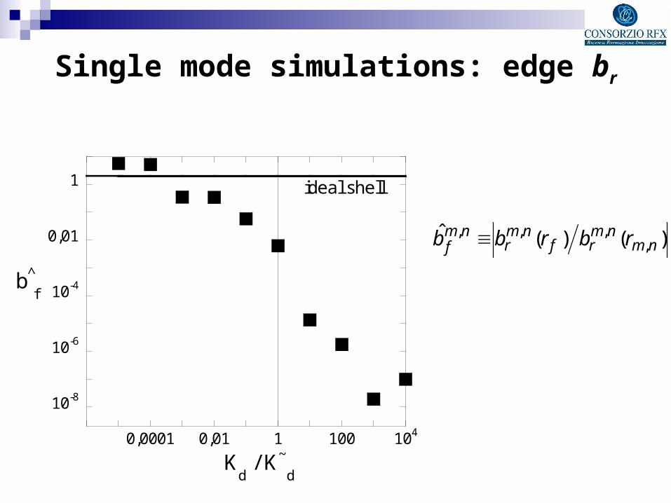
Single mode simulations: edge br
)()(ˆ,
,,,nm
nmrf
nmr
nmf rbrbb
10-8
10-6
10-4
0,01
1
0,0001 0,01 1 100 104
Kd / K~
d
b^
f
ideal shell

Multi-mode simulations: frequencies
1000
104
105
7 9 11 13 15 17 19
1 3 5 7 9 11
d1,n/dt
m=1
d0,n/dt
m=0
rad
/s
n (m=1)
n (m=0)
Averages over the second half of the simulation

Multi-mode simulations: plasma surface distortion
0
2,5x10⁻⁴
5x10⁻⁴
0 0,002 0,004 0,006 0,008
max[1
max[0
(cm
)
time(s)

Multi-mode simulations: no phase-locking
Ideal shell feedback
1,11,1 nn

Multi-mode simulations: no phase-locking
dt
d
dt
d
dt
d nnnn 1
,11,1
1,11,1
nn
nn
dt
d
dt
d ,10
,11,1
0
1,1
Incompatible with

Internal coils: discrete feedback stable solutions
10-5
0,0001
0,001
0,01
10-7 10-6 10-5 0,0001
K~
d / K~
d+
t(s)

Internal coils: discrete feedback stable solutions
0,01
0,1
1
10-5 0,0001 0,001 0,01
b^ f
K~
d / K~
d+
ideal shell limit
b)

The MHD model: Ψwi, Ψwe
wewi
nmnm
rrrrt
,;2
,2,
0
Boundary conditions from Newcomb’s solution

The MHD model: Ψs
)(,,0
, )()( tnminms
nms ett
trmtrndt
dnmnm
nm
,, ,,
,
From experiment
No-slip condition

The MHD model: Ωθ, ΩΦ
nmnm
nmEM rrrR
TS
rr
rrt ,
0
30
2
,
4
1
04
1,
00
32
,3
3
nm
nm
nmEM
Drr
Rr
T
n
mS
rr
rrt

The MHD model: δTEM
nmnmnmnmnm cskji
nmnmnm
nmk
nmj
nmi
nms
nmc
nm
nmcsnm
EM
kji
R
rnm
EnRT
,2,21,12,2,1,1 ,,,
,2,2,1,1
2,21,1,
,,
20
2,22
,
0
02
,
,,Im
Im8

The MHD model: Ψc
nmcc
cr
cr
nm InmR
cnmi
rr ,
20
222
0, ),(
Further variable: Icm,n

The MHD model: Ic
termsaddIIdt
dI nmf
nmc
nmcnm
c .,Re
,,
,
Further variable: IREFm,n
RL equation for the plasma-coils coupled system
rjijic
REFjicji dt
dIRIRV ,,,,

The MHD model: IREF
nmr
nmd
nmref w
dt
dKI ,,,
Acquired by the feedback

Why a pure derivative control?
When | cm,n|>>1, from the RL equation one gets
nmc
nmc
nmc
nmc
nmf IiIiI ,,,,,
Re 1
nmrnm
c
nmdnm
c wK
I ,,
,,
nmr
nmd
nmf wKiI ,,,
Re


