Full Terms & Conditions of access and use can be found at http://www.tandfonline.com/action/journalInformation?journalCode=glma20 Download by: [Hong Kong Polytechnic University] Date: 30 March 2016, At: 21:26 Linear and Multilinear Algebra ISSN: 0308-1087 (Print) 1563-5139 (Online) Journal homepage: http://www.tandfonline.com/loi/glma20 Perturbation bounds of tensor eigenvalue and singular value problems with even order Maolin Che, Liqun Qi & Yimin Wei To cite this article: Maolin Che, Liqun Qi & Yimin Wei (2016) Perturbation bounds of tensor eigenvalue and singular value problems with even order, Linear and Multilinear Algebra, 64:4, 622-652, DOI: 10.1080/03081087.2015.1074153 To link to this article: http://dx.doi.org/10.1080/03081087.2015.1074153 Published online: 14 Aug 2015. Submit your article to this journal Article views: 66 View related articles View Crossmark data
Transcript
Full Terms & Conditions of access and use can be found athttp://www.tandfonline.com/action/journalInformation?journalCode=glma20
Download by: [Hong Kong Polytechnic University] Date: 30 March 2016, At: 21:26
Perturbation bounds of tensor eigenvalue andsingular value problems with even order
Maolin Che, Liqun Qi & Yimin Wei
To cite this article: Maolin Che, Liqun Qi & Yimin Wei (2016) Perturbation bounds of tensoreigenvalue and singular value problems with even order, Linear and Multilinear Algebra, 64:4,622-652, DOI: 10.1080/03081087.2015.1074153
To link to this article: http://dx.doi.org/10.1080/03081087.2015.1074153
Linear and Multilinear Algebra, 2016Vol. 64, No. 4, 622–652, http://dx.doi.org/10.1080/03081087.2015.1074153
Perturbation bounds of tensor eigenvalue and singular value problemswith even order
Maolin Chea, Liqun Qib and Yimin Weic∗
aSchool of Mathematical Sciences, Fudan University, Shanghai, P.R. China; bDepartment ofApplied Mathematics, The Hong Kong Polytechnic University, Kowloon, Hong Kong; cSchool of
Mathematical Sciences and Shanghai Key Laboratory of Contemporary Applied Mathematics,Fudan University, Shanghai, P.R. China
Communicated by R. Li
(Received 3 February 2015; accepted 5 July 2015)
The main purpose of this paper is to investigate the perturbation bounds ofthe tensor eigenvalue and singular value problems with even order. Weextend classical definitions from matrices to tensors, such as, λ-tensor and thetensor polynomial eigenvalue problem. We design a method for obtaining amode-symmetric embedding from a general tensor. For a given tensor, if thetensor is mode-symmetric, then we derive perturbation bounds on an algebraicsimple eigenvalue and Z-eigenvalue. Otherwise, based on symmetric or mode-symmetric embedding, perturbation bounds of an algebraic simple singular valueare presented. For a given tensor tuple, if all tensors in this tuple are mode-symmetric, based on the definition of a λ-tensor, we estimate perturbation boundsof an algebraic simple polynomial eigenvalue. In particular, we focus on tensorgeneralized eigenvalue problems and tensor quadratic eigenvalue problems.
Qi [1] defined two kinds of eigenvalue and investigated relative results similar to the matrixeigenvalue. Independently, Lim [2] proposed another definition of eigenvalue, eigenvectors,singular value and singular vectors for tensors based on a constrained variational approach,much like the Rayleigh quotient for symmetric matrix eigenvalue (see [3, Chapter 8]).
Chang et al. [4,5] introduced the eigenvalue and defined generalized tensor eigenprob-lems. To our best knowledge, Kolda and Mayo [6], Cui et al. [7] proposed two algorithmsfor solving generalized tensor eigenproblems, and they pointed out that the generalizedeigenvalue framework unifying definitions of tensor eigenvalue, such as, eigenvalue andH-eigenvalue [1,2], E-eigenvalue, Z-eigenvalue [1] and D-eigenvalue [8]. Ding and Wei
[9] focused on the properties and perturbations of the spectra of regular tensor pairs andextended results from matrices or matrix pairs to tensor pairs.
Li and Ng [10,11] extended the well-known column sum bound of the spectral radiusfor nonnegative matrices to the tensor case, and also derived an upper bound of the spectralradius for a nonnegative tensor via the largest eigenvalue of a symmetric tensor.
Throughout this paper, we assume that m, n (≥ 2) are positive integers and m is even.We use small letters x, u, v, . . . , for scalars, small bold letters x, u, v, . . . , for vectors,capital letters A, B, C, . . . , for matrices and calligraphic letters A,B, C, . . . , for tensors.Denote [n] by {1, 2, . . . , n}. Denote 〈n〉 by {n1, n2, . . . , nm}.
The set Tm,n consists of all order m dimension n tensors and each element of A ∈ Tm,n
is real, that is, Ai1i2...im ∈ R where ik ∈ [n] with k ∈ [m], and the set Tm,〈n〉 consists of allorder m tensors of size n1 × n2 × · · · × nm and each element of A ∈ Tm,〈n〉 is real, that is,Ai1i2...im ∈ R where ik ∈ [nk] with k ∈ [m]. For a vector x ∈ C
n , ‖x‖2 = x∗x where ‘∗’represents conjugate transposition, |x|mm means xm
1 + xm2 + · · · + xm
n . In particular, whenx ∈ Rn , the vector m-norm for |x|mm is ‖x‖m
m = |x1|m + |x2|m + · · · + |xn|m . 0 means thezero vector in C
n .A ∈ Tm,n is nonnegative (see [4]), if all elements are nonnegative, and we denote
nonnegative tensors by N Tm,n . D ∈ Tm,n is diagonal (see [1]), if all off-diagonal entriesare zero. In particular, if the diagonal entries of D are 1, then D is called the identity tensor(see [1]) and denote it by I.
The rest of our paper is organized as follows. Section 2 introduces some definitions,such as mode-k determinant, the polynomial tensor eigenvalue problem, from matrices totensors, derives a method for obtaining mode-symmetric embedding from A ∈ Tm,〈n〉,and covers a classical result about the perturbation of a simple eigenvalue of A ∈ C
n×n . InSection 3, for a mode-symmetric tensor, we derive some perturbation bounds of an algebraicsimple eigenvalue and Z-eigenvalue, based on symmetric or mode-symmetric embedding,we explore the perturbation bounds of an algebraic simple singular value of A ∈ Tm,〈n〉.In Section 4, for a given λ-tensor, we derive the first-order perturbation of an algebraicsimple polynomial eigenvalue and obtain the coefficient of the first-order perturbation term.In particular, we consider the tensor generalized eigenvalue problem, and present a newperturbation bound of an algebraic simple eigenvalue. We show ill-condition tensors forcomputing Z-eigenvalue or singular value via random numerical examples. We concludeour paper in Section 6.
2. Preliminaries
In this section, we present several definitions generalized from matrices to tensors, we statesome remarks and properties associated with these definitions. We shall recall a lemmaabout the perturbation of a simple eigenvalue of a matrix A ∈ C
n×n .
2.1. Definitions
The mode-k product (see [12,13]) of a tensor A ∈ Tm,n by a matrix B ∈ Rn×n , denoted by
A ×k B is a tensor C ∈ Tm,n ,
Ci1...ik−1 j ik+1...im =n∑
ik=1
Ai1...ik−1ik ik+1...im b jik , k ∈ [m].
Dow
nloa
ded
by [
Hon
g K
ong
Poly
tech
nic
Uni
vers
ity]
at 2
1:26
30
Mar
ch 2
016
624 M. Che et al.
In particular, the mode-k multiplication of a tensor A ∈ Tm,n by a vector x ∈ Rn is
denoted by A×kx. When we set C = A×kx, by elementwise, we have
Ci1...ik−1ik+1...im =n∑
ik=1
Ai1...ik−1ik ik+1...im xik .
Let m vectors xk ∈ Rn , A×1x1 . . . ×mxm is easy to define. If these m vectors are also the
same vectors, denoted by x, then A×1x . . . ×mx can be simplified as Axm . The mode-kproduct of a tensor A ∈ Tm,〈n〉 by a matrix B ∈ R
p×nk is easy to define.The Frobenius norm of a tensor A ∈ Tm,〈n〉 (see [13,14]) is the square root of the sum
of the squares of all its elements, i.e.
‖A‖F =√√√√ n1∑
i1=1
n2∑i2=1
· · ·nm∑
im=1
A2i1i2...im
,
which is a generalization of the well-known Frobenius-norm of a matrix A ∈ Cm×n .
Analogous to the reducible matrices (see [15, Chapter 2]), A ∈ Tm,n is called reducible(see [4]), if there exists a nonempty proper index subset I ⊂ {1, 2, . . . , n} such that
Ai1i2...im = 0, for all i1 ∈ I and i2, . . . , im /∈ I.
If A is not reducible, then we call A irreducible.A is called symmetric (see [1,2]) if Ai1i2...im is invariant by any permutation π , that is,
Ai1i2...im = Aπ(i1,i2,...,im ), where all ik ∈ [n] with k ∈ [m]. We denote all symmetric tensorsby STm,n .
Symmetric tensor is a special case of the following definition of ‘mode-symmetric’. Weshall provide a more general definition about mode-symmetric of a tensor.
Definition 2.1 Let A ∈ Tm,n. A is called mode-symmetric, if its entries satisfy thefollowing formulae
2 , . . . , xm−1n ), then the pair (λk, xk) is called a mode-k
eigenpair of A.If xk ∈ R
n and λk ∈ R, then the pair (λk, xk) is called a mode-k H-eigenpair of A.Moreover, the mode-k spectrum σk(A) of A is defined as
σk(A) = {λ|λ is a mode-k eigenvalue of A}.
The mode-k spectral radius ρk(A) is max{|λ| | λ ∈ σk(A)}. While the spectral radiusρ(A) of a tensor A is denoted by ρ(A) = max1≤k≤m ρk(A).
Mode-k eigenvectors are generalized by left and right eigenvectors of a matrixA ∈ Rn×n . For k ∈ [m], some properties of the mode-k eigenpairs of A are presentedin the following:
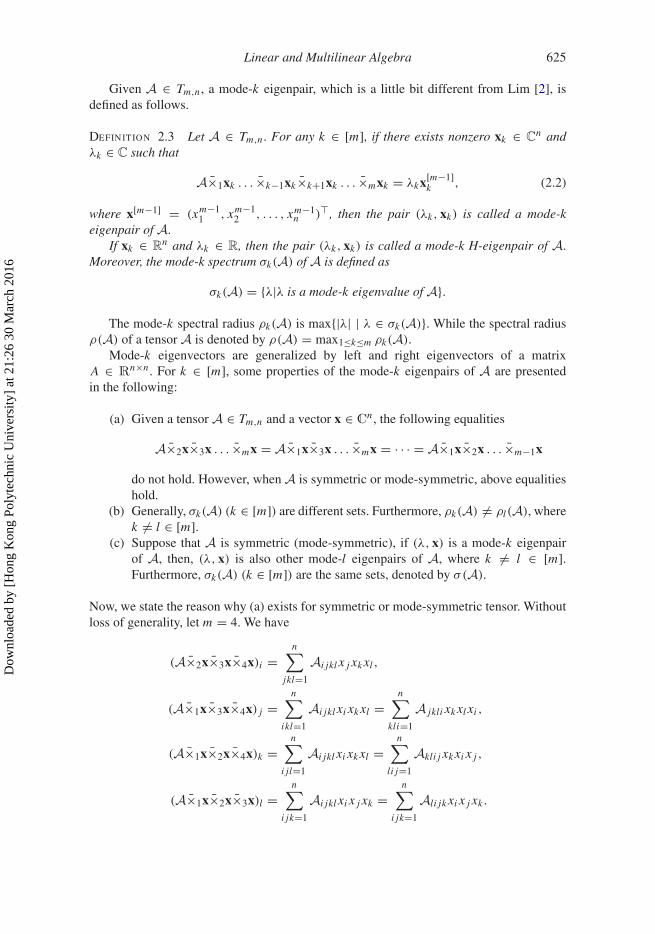
(a) Given a tensor A ∈ Tm,n and a vector x ∈ Cn , the following equalities
do not hold. However, when A is symmetric or mode-symmetric, above equalitieshold.
(b) Generally, σk(A) (k ∈ [m]) are different sets. Furthermore, ρk(A) �= ρl(A), wherek �= l ∈ [m].
(c) Suppose that A is symmetric (mode-symmetric), if (λ, x) is a mode-k eigenpairof A, then, (λ, x) is also other mode-l eigenpairs of A, where k �= l ∈ [m].Furthermore, σk(A) (k ∈ [m]) are the same sets, denoted by σ(A).
Now, we state the reason why (a) exists for symmetric or mode-symmetric tensor. Withoutloss of generality, let m = 4. We have
(A×2x×3x×4x)i =n∑
jkl=1
Ai jkl x j xk xl ,
(A×1x×3x×4x) j =n∑
ikl=1
Ai jkl xi xk xl =n∑
kli=1
A jkli xk xl xi ,
(A×1x×2x×4x)k =n∑
i jl=1
Ai jkl xi xk xl =n∑
li j=1
Akli j xk xi x j ,
(A×1x×2x×3x)l =n∑
i jk=1
Ai jkl xi x j xk =n∑
i jk=1
Ali jk xi x j xk .
Dow
nloa
ded
by [
Hon
g K
ong
Poly
tech
nic
Uni
vers
ity]
at 2
1:26
30
Mar
ch 2
016
626 M. Che et al.
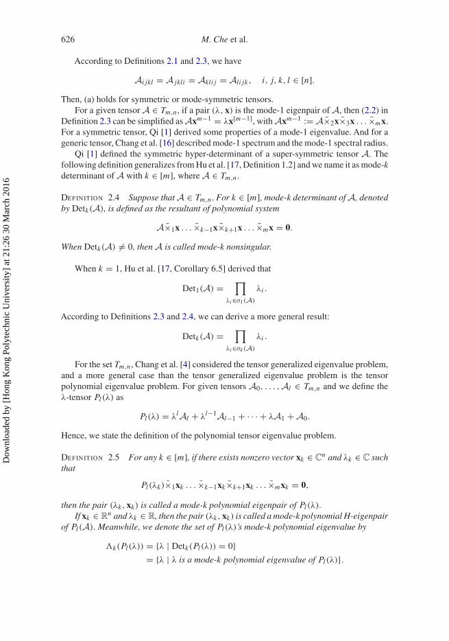
According to Definitions 2.1 and 2.3, we have
Ai jkl = A jkli = Akli j = Ali jk, i, j, k, l ∈ [n].Then, (a) holds for symmetric or mode-symmetric tensors.
For a given tensor A ∈ Tm,n , if a pair (λ, x) is the mode-1 eigenpair of A, then (2.2) inDefinition 2.3 can be simplified as Axm−1 = λx[m−1], with Axm−1 := A×2x×3x . . . ×mx.For a symmetric tensor, Qi [1] derived some properties of a mode-1 eigenvalue. And for ageneric tensor, Chang et al. [16] described mode-1 spectrum and the mode-1 spectral radius.
Qi [1] defined the symmetric hyper-determinant of a super-symmetric tensor A. Thefollowing definition generalizes from Hu et al. [17, Definition 1.2] and we name it as mode-kdeterminant of A with k ∈ [m], where A ∈ Tm,n .
Definition 2.4 Suppose that A ∈ Tm,n. For k ∈ [m], mode-k determinant of A, denotedby Detk(A), is defined as the resultant of polynomial system
A×1x . . . ×k−1x×k+1x . . . ×mx = 0.
When Detk(A) �= 0, then A is called mode-k nonsingular.
When k = 1, Hu et al. [17, Corollary 6.5] derived that
Det1(A) =∏
λi ∈σ1(A)
λi .
According to Definitions 2.3 and 2.4, we can derive a more general result:
Detk(A) =∏
λi ∈σk (A)
λi .
For the set Tm,n , Chang et al. [4] considered the tensor generalized eigenvalue problem,and a more general case than the tensor generalized eigenvalue problem is the tensorpolynomial eigenvalue problem. For given tensors A0, . . . ,Al ∈ Tm,n and we define theλ-tensor Pl(λ) as
Pl(λ) = λlAl + λl−1Al−1 + · · · + λA1 + A0.
Hence, we state the definition of the polynomial tensor eigenvalue problem.
Definition 2.5 For any k ∈ [m], if there exists nonzero vector xk ∈ Cn and λk ∈ C such
that
Pl(λk)×1xk . . . ×k−1xk×k+1xk . . . ×mxk = 0,
then the pair (λk, xk) is called a mode-k polynomial eigenpair of Pl(λ).If xk ∈ R
n and λk ∈ R, then the pair (λk, xk) is called a mode-k polynomial H-eigenpairof Pl(A). Meanwhile, we denote the set of Pl(λ)’s mode-k polynomial eigenvalue by
�k(Pl(λ)) = {λ | Detk(Pl(λ)) = 0}= {λ | λ is a mode-k polynomial eigenvalue of Pl(λ)}.
Dow
nloa
ded
by [
Hon
g K
ong
Poly
tech
nic
Uni
vers
ity]
at 2
1:26
30
Mar
ch 2
016
Linear and Multilinear Algebra 627
Ding et al. [18] defined a regular tensor pair (A,B) with A,B ∈ Tm,n . In general,according to Definition 2.4 and λ-tensor Pl(λ), mode-k regular about a tensor (l + 1)-tupleis defined as follows.
Definition 2.6 For a given λ-tensor Pl(λ), a tensor (l + 1)-tuple (Al , . . . ,A1,A0) ismode-k singular if for all λ, Detk(Pl(λ)) ≡ 0 holds, where all tensors in this tuple belongto Tm,n, or if all tensors in this tuple belong to Tm,〈n〉, where these exist two different indicesk, l ∈ [m] such that nk �= nl . Otherwise the (l + 1)-tuple (Al , . . . ,A1,A0) is said to bemode-k regular, where all tensors in the tuple belong to Tm,n.
In this paper, we only consider the tensor polynomial eigenvalue problem where as-sociated tensor (l + 1)-tuple (Al , . . . ,A1,A0) is regular. Meanwhile, for a given mode-kregular tensor tuple, according to Definition 2.6, we know that there exists a λ such thatDetk(Pl (λ)) �= 0. Then, we can choice another (l + 1)-tuple (Al , . . . , A1, A0) such thatAl = ∑l
i=0 λlAl and there is a one-to-one map between �k(Pl(λ)) and �k(Pl(λ)), whereDetk(Al) �= 0 and Pl(λ) = λlAl + λl−1Al−1 + · · · + λA1 + A0.
Furthermore, we can also suppose that Detk(Al) �= 0, that is, Al is nonsingular. Fora given Pl(λ), when Al is nonsingular, we will show that, for all k ∈ [m], �k(Pl(λ)) arefinite subsets of C.
Meanwhile, for a given tensor (l + 1)-tuple (Al , . . . ,A1,A0), we can also define a(α, β)-tensor. Let Pl(α, β) = αlAl + αl−1βAl−1 + · · · + αβl−1A1 + βlA0. It is obviousthat Pl(α, β) is a homogeneous polynomial on α and β. The relationship between Pl(λ)
and Pl(α, β) is listed below. If β �= 0, then Pl(α, β) = βl Pl(α/β); and if α �= 0, thenPl(α, β) = αl Pl(β/α), where Pl(β/α) = Al + tAl−1 +· · ·+ t l−1A1 + t lA0 and t = β/α.
For a given λ-tensor Pl(λ), when the pair (λk, xk) is a mode-k polynomial eigenpair ofPl(λ), then, we can choose a pair (αk, βk) such that
Pl(αk, βk)×1xk . . . ×k−1xk×k+1xk . . . ×mxk = 0
and
λk ={
αk/βk, βk �= 0,
∞, βk = 0,
with (αk, βk) �= (0, 0).For a given tensor A ∈ Tm,〈n〉, let xk ∈ R
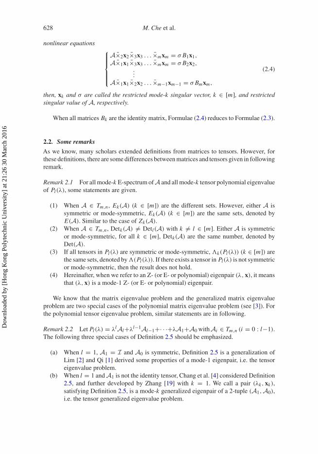
nk be nonzero vectors and ‖xk‖ = 1 withk ∈ [m]. If (σ, x1, x2, . . . , xm) is a solution of this following nonlinear equations⎧⎪⎪⎪⎨⎪⎪⎪⎩
A×2x2×3x3 . . . ×mxm = σx1,
A×1x1×3x3 . . . ×mxm = σx2,...
A×1x1×2x2 . . . ×m−1xm−1 = σxm,
(2.3)
then, the unit vector xk and σ are called the mode-k singular vector, k ∈ [m], and singularvalue of A, respectively (see [2]).
Meanwhile, for a given tensor A ∈ Tm,〈n〉, its singular value and associated mode-ksingular vectors can be generalized the in following form.
Definition 2.7 Let Bk ∈ Rnk×nk be positive definite matrices and xk ∈ R
nk be nonzerovectors where x
k Bkxk=1 with k ∈ [m]. If (σ, x1, x2, . . . , xm) is a solution of this following
then, xk and σ are called the restricted mode-k singular vector, k ∈ [m], and restrictedsingular value of A, respectively.
When all matrices Bk are the identity matrix, Formulae (2.4) reduces to Formulae (2.3).
2.2. Some remarks
As we know, many scholars extended definitions from matrices to tensors. However, forthese definitions, there are some differences between matrices and tensors given in followingremark.
Remark 2.1 For all mode-k E-spectrum of A and all mode-k tensor polynomial eigenvalueof Pl(λ), some statements are given.
(1) When A ∈ Tm,n , Ek(A) (k ∈ [m]) are the different sets. However, either A issymmetric or mode-symmetric, Ek(A) (k ∈ [m]) are the same sets, denoted byE(A). Similar to the case of Zk(A).
(2) When A ∈ Tm,n , Detk(A) �= Detl(A) with k �= l ∈ [m]. Either A is symmetricor mode-symmetric, for all k ∈ [m], Detk(A) are the same number, denoted byDet(A).
(3) If all tensors in Pl(λ) are symmetric or mode-symmetric, �k(Pl(λ)) (k ∈ [m]) arethe same sets, denoted by �(Pl(λ)). If there exists a tensor in Pl(λ) is not symmetricor mode-symmetric, then the result does not hold.
(4) Hereinafter, when we refer to an Z- (or E- or polynomial) eigenpair (λ, x), it meansthat (λ, x) is a mode-1 Z- (or E- or polynomial) eigenpair.
We know that the matrix eigenvalue problem and the generalized matrix eigenvalueproblem are two special cases of the polynomial matrix eigenvalue problem (see [3]). Forthe polynomial tensor eigenvalue problem, similar statements are in following.
Remark 2.2 Let Pl(λ) = λlAl+λl−1Al−1+· · ·+λA1+A0 with Ai ∈ Tm,n (i = 0 : l−1).The following three special cases of Definition 2.5 should be emphasized.
(a) When l = 1, A1 = I and A0 is symmetric, Definition 2.5 is a generalization ofLim [2] and Qi [1] derived some properties of a mode-1 eigenpair, i.e. the tensoreigenvalue problem.
(b) When l = 1 and A1 is not the identity tensor, Chang et al. [4] considered Definition2.5, and further developed by Zhang [19] with k = 1. We call a pair (λk, xk),satisfying Definition 2.5, is a mode-k generalized eigenpair of a 2-tuple (A1,A0),i.e. the tensor generalized eigenvalue problem.
Dow
nloa
ded
by [
Hon
g K
ong
Poly
tech
nic
Uni
vers
ity]
at 2
1:26
30
Mar
ch 2
016
Linear and Multilinear Algebra 629
Figure 1. Intuitive performance of msym(A): A1 for the first part, the second part represented byA2; and A3 for the third part. Not labelled part means all zero elements of msym(A).
(c) When l = 2, We call a pair (λk, xk), satisfying Definition 2.5, is a mode-k quadraticeigenpair of a 3-tuple (A2,A1,A0), i.e. the tensor quadratic eigenvalue problem.
Some properties of the mode-k tensor matrix product are given as follows.
Lemma 2.1 ([14, Property 2 and 3], [13]) Given a tensor A ∈ Tm,n and the matricesF ∈ R
n×n and G ∈ Rn×n. For different integers k and l, one has
(A ×k F) ×l G = (A ×l G) ×k F = A ×k F ×l G, (A ×k F) ×k G = A ×k (G · F),
where ‘·’ means the multiplication of two matrices.
Suppose that A ∈ Cn×n . Wilkinson [20], Demmel [21] and Stewart and Sun [22]
concentrated on computing the condition number of a simple eigenvalue, respectively.
Lemma 2.2 ([21, Theorem 4.4], [22, Theorem 2.3]) Let λ be a simple eigenvalue of Awith right eigenvector x and left eigenvector y, normalized so that ‖x‖ = ‖y‖ = 1. Letλ + δλ be the corresponding eigenvalue of A + δA. Then
δλ = y∗δAxy∗x
+ O(‖δA‖22), or
|δλ| ≤ ‖δA‖2
y∗x+ O(‖δA‖2
2) = sec (y, x)‖δA‖2 + O(‖δA‖22),
Dow
nloa
ded
by [
Hon
g K
ong
Poly
tech
nic
Uni
vers
ity]
at 2
1:26
30
Mar
ch 2
016
630 M. Che et al.
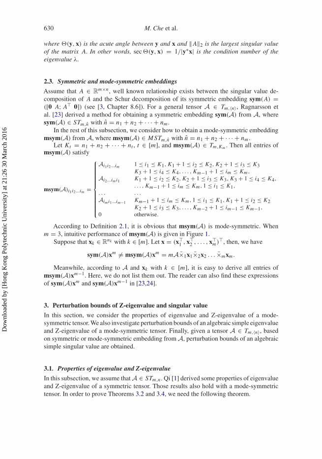
where (y, x) is the acute angle between y and x and ‖A‖2 is the largest singular valueof the matrix A. In other words, sec (y, x) = 1/|y∗x| is the condition number of theeigenvalue λ.
2.3. Symmetric and mode-symmetric embeddings
Assume that A ∈ Rm×n , well known relationship exists between the singular value de-
composition of A and the Schur decomposition of its symmetric embedding sym(A) =([0 A; A 0]) (see [3, Chapter 8.6]). For a general tensor A ∈ Tm,〈n〉, Ragnarsson etal. [23] derived a method for obtaining a symmetric embedding sym(A) from A, wheresym(A) ∈ STm,n with n = n1 + n2 + · · · + nm .
In the rest of this subsection, we consider how to obtain a mode-symmetric embeddingmsym(A) from A, where msym(A) ∈ M STm,n with n = n1 + n2 + · · · + nm .
Let Kt = n1 + n2 + · · · + nt , t ∈ [m], and msym(A) ∈ Tm,Km . Then all entries ofmsym(A) satisfy
According to Definition 2.1, it is obvious that msym(A) is mode-symmetric. Whenm = 3, intuitive performance of msym(A) is given in Figure 1.
Suppose that xk ∈ Rnk with k ∈ [m]. Let x = (x
1 , x2 , . . . , x
m), then, we have
sym(A)xm �= msym(A)xm = mA×1x1×2x2 . . . ×mxm .
Meanwhile, according to A and xk with k ∈ [m], it is easy to derive all entries ofmsym(A)xm−1. Here, we do not list them out. The reader can also find these expressionsof sym(A)xm and sym(A)xm−1 in [23,24].
3. Perturbation bounds of Z-eigenvalue and singular value
In this section, we consider the properties of eigenvalue and Z-eigenvalue of a mode-symmetric tensor. We also investigate perturbation bounds of an algebraic simple eigenvalueand Z-eigenvalue of a mode-symmetric tensor. Finally, given a tensor A ∈ Tm,〈n〉, basedon symmetric or mode-symmetric embedding from A, perturbation bounds of an algebraicsimple singular value are obtained.
3.1. Properties of eigenvalue and Z-eigenvalue
In this subsection, we assume that A ∈ STm,n . Qi [1] derived some properties of eigenvalueand Z-eigenvalue of a symmetric tensor. Those results also hold with a mode-symmetrictensor. In order to prove Theorems 3.2 and 3.4, we need the following theorem.
Dow
nloa
ded
by [
Hon
g K
ong
Poly
tech
nic
Uni
vers
ity]
at 2
1:26
30
Mar
ch 2
016
Linear and Multilinear Algebra 631
Theorem 3.1 Assume that A is a mode-symmetric tensor and m is even. The followingconclusions holds for A:
(a) A always has H-eigenvalue. A is positive definite (positive semidefinite) if and onlyif all of its H-eigenvalue are positive (nonnegative).
(b) A always has Z-eigenvalue. A is positive definite (positive semidefinite) if and onlyif all of its Z-eigenvalue are positive (nonnegative).
Proof Firstly, we prove part (a). We see (2.2) is the optimality condition of
max
{Axm :
n∑i=1
xmi = 1, x ∈ R
n
}(3.1)
and
min
{Axm :
n∑i=1
xmi = 1, x ∈ R
n
}. (3.2)
As the feasible set is compact and the objective function is continuous, the global maximizerand minimizer always exist. This shows that (2.2) has real solutions, i.e. A always has H-eigenvalue. Since A is positive definite (positive semidefinite) if and only if the optimalvalue of (3.1) is positive (nonnegative), we draw the second conclusion of (a).
Now, we will prove part (b). The proof of (b) is similar to the proof of (a), as long aswe replace by
max
{Axm :
n∑i=1
xmi = 1, x ∈ R
n
}and
min
{Axm :
n∑i=1
xmi = 1, x ∈ R
n
}.
�
3.2. Algebraic simple Z-eigenvalue
Suppose that A ∈ M STm,n . Since m is even, then there exists a positive integer h suchthat m = 2h. Denote by E the tensor I ⊗ I ⊗ · · · ⊗ I︸ ︷︷ ︸
h
. A always has Z-eigenvalue (see [1,
Theorem 5]), if λ is an Z-eigenvalue of A, it is known that λ is a root of Det(A − λE) = 0(see [1, Theorem 2]).
It is observed (see [25]) that the complex E-eigenpairs of a tensor form the equivalenceclass under a multiplicative transformation. That is (see [26]), if (λ, x) is an E-eigenpair ofA and y = eιϕx with ϕ ∈ R, where ι = √−1 then y∗y = x∗x = 1 and
Therefore, (eι(m−2)ϕλ, eιϕx) is also an E-eigenpair of A for any ϕ ∈ R. Then, we can chooseϕ∗ such that (eι(m−2)ϕ∗λ, eιϕ∗x) is a Z-eigenpair. Hence, without loss of generality, we onlyconsider the perturbation bounds of a Z-eigenvalue of a symmetric or mode-symmetrictensor.
Dow
nloa
ded
by [
Hon
g K
ong
Poly
tech
nic
Uni
vers
ity]
at 2
1:26
30
Mar
ch 2
016
632 M. Che et al.
Chang et al. [4] defined the geometric multiplicity of an eigenvalue λ, meanwhile,Hu et al. [17] considered the algebraic multiplicity of an eigenvalue λ. Similarly, we candefine the geometric and algebraic multiplicity of an Z-eigenvalue. An algebraic simple Z-eigenvalue is defined as an Z-eigenvalue whose algebraic multiplicity is one. This definitionis applicable to a generalized eigenvalue, a polynomial eigenvalue and a singular value. Wepresent the perturbation bound of an algebraic simple Z-eigenvalue λ of A + εB.
Theorem 3.2 Suppose A,B ∈ M STm,n and ε ∈ R. Let (λ, x) be an algebraic simpleZ-eigenpair of A. Then there exists ε0 > 0 and an analytic function λ(ε) with |ε| ≤ ε0 suchthat
λ(0) = λ, λ′(0) = dλ
dε
∣∣∣∣ε=0
= Bxm,
with xx = 1. Therefore, λ(ε) is an algebraic simple Z-eigenvalue of A+εB over |ε| ≤ ε0,and
λ(ε) = λ + εBxm + O(ε2).
Proof When A is symmetric, we know that A always has Z-eigenvalue (see [1, Theorem5]), that is, Z(A) is the nonempty set. This result also holds when A is mode-symmetric(see Theorem 3.1).
By the description of Qi [1], the E-characteristic polynomial of A + εB becomes
ϕε(z) = Det(zE − A − εB).
It is obvious that ϕε(z) is an analytic function associated to ε and z. Define Dr := {z ∈ C :|z − λ| ≤ r}. Let r be arbitrarily small such that Z(A) ∩ Dr = {λ}. Denote the boundaryof Dr as ∂Dr . Then minz∈∂Dr |ϕ0(z)| = γ > 0.
Since ϕε(z) is a continuous function of ε, then there exists ε0 > 0, such that for all ε
with |ε| ≤ ε0, ϕε(z) has only one zero point in Dr and minz∈∂Dr|ε|≤ε0
|ϕε(z)| > 0.
It follows from the Residue Theorem (see [27]) that the zero point λ(ε) of ϕε(z) in Dr
can be represented as λ(ε) = 12π
∮∂Dr
zϕ′ε(z)
ϕε(z)dz, where ϕ′
ε(z) = dϕε(z)/dz.
Noting that zϕ′ε(z)
ϕε(z)and d
dz
(zϕ′
ε(z)ϕε(z)
)are continuous on ∂Dr , by the differential and integral
order exchange theorem, λ(ε) is an analytic function, if |ε| ≤ ε0. Hence, λ(ε) can beexpressed as
λ(ε) = λ(0) + λ′(0)ε + O(ε2), λ(0) = λ, |ε| ≤ ε0.
For an algebraic simple Z-eigenvalue λ of a mode-symmetric tensor A, if there exist tworeal vectors x1 and x2 such that
Axm−1i = λxi , x
i xi = 1, i ∈ [2],then, it is obvious that if x1 = cx2, then c satisfies that c2 = 1 and cm−2 = 1. In this case,we can see that x1 and x2 are the same vectors, otherwise, we see that x1 and x2 are thedifferent vectors. Hence, we denote
δ = min{‖y − x‖ : y and x are the different eigenvectors associated with λ}.Then, over {z ∈ Cn : ‖z − x‖ < δ}, there exists a unique eigenvector x of A associated toλ. (For an algebraic simple Z-eigenvalue λ, if its geometric multiplicity is also 1, then setδ ≤ ε0.)
Dow
nloa
ded
by [
Hon
g K
ong
Poly
tech
nic
Uni
vers
ity]
at 2
1:26
30
Mar
ch 2
016
Linear and Multilinear Algebra 633
For an algebraic simple Z-eigenvalue λ(ε) of A+ εB, since λ(ε) is an analytic functionwith |ε| ≤ ε0, then there exists δ = min{δ, ε0} such that ‖x(ε) − x‖ < δ and x(ε) isthe unique eigenvector of A + εB corresponding to λ(ε). According to some results aboutalgebraic functions (see [28]), we derive that x(ε) is an analytic function, where |ε| ≤ δ
and x(0) = x.As (A+εB)x(ε)m−1 = λ(ε)x(ε), by differentiating this equation with respect to ε, and
setting ε = 0, we have
Ax + Bx(0)m−1 = λ′(0)x(0) + λ(0)x′(0),
where Ax = A(×2x′(0)×3x(0) . . . ×mx(0) + · · · + ×2x(0) . . . ×m−1x(0)×mx′(0)).Since (λ, x) is a mode-k Z-eigenpair and ‖x‖ = 1, then
λ′(0) = Bx(0)m = Bxm .
Hence, this theorem is complete proved. �
Gohberg and Koltracht [29] studied condition numbers of maps in finite-dimensionalspaces F : R
p → Rq . The condition number of F at a point a ∈ DF characterizes the
instantaneous rate of change in F(a) with respect to perturbations in a.Then, another perturbation result of an nonzero algebraic simple Z-eigenvalue λ = λ(A)
is considered, whose associated eigenvector x is a real nonzero vector with ‖x‖ = 1. It iswell known that the map FE : ε → λ(A + εB) is analytic in a neighbourhood of 0 (see[17]). Therefore, the map F : A → λ(A) has continuous partial derivatives with respect toeach entry at A and
∂ F
∂i1i2...im
(A) := limt→0
F(A + tJ ) − F(A)
t= xi1 xi2 . . . xim ,
where J is the zero tensor except for Ji1i2...im = 1. Here, we give an example to illustratethe meaning of J . Without loss of generality, let m = 4 and (i1, i2, i3, i4) = (1, 2, 3, 4),then J can be written as J = e1 ◦ e2 ◦ e3 ◦ e4 where ei is the i th column of the n × nidentity matrix with i ∈ [4]. Then, all entries of J are given in following:
J j1 j2 j3 j4 = e1( j1)e2( j2)e3( j3)e4( j4),
where jk ∈ [n] and ek( jk) is the jk th element of ek with k ∈ [4]. In general, J = ei1 ◦ ei2 ◦· · · ◦ eim where eik is the ik th column of the n × n identity matrix with k ∈ [m].
Hence, as a map from Rnm → R, F is differentiable at A and
F ′(A) =[
∂ F
∂11...1, . . . ,
∂ F
∂11...1n,
∂ F
∂21...1, . . . ,
∂ F
∂nn...n
].
According to a formula by Gohberg and Koltracht [29], for relatively small componen-twise perturbations in A, i.e.
|Ei1i2...im | ≤ ε|Ai1i2...im |, ik ∈ [n], k ∈ [m],where E ∈ M STm,n and ε > 0 is arbitrarily small, the sensitivity of F(A) is characterizedby the componentwise condition number of F at A is
Dow
nloa
ded
by [
Hon
g K
ong
Poly
tech
nic
Uni
vers
ity]
at 2
1:26
30
Mar
ch 2
016
634 M. Che et al.
c(F,A) = ‖F ′(A)DA‖∞‖F(A)‖∞
,
where DA = diag(A11...1, . . . ,A11...1n,A21...1, . . . ,Ann...n), and λ �= 0.It indicates that
where an absolute value of a tensor is the corresponding tensor of the absolute values of itsentries. Thus, if E is a perturbation of A, then we have a relative perturbation bound of anonzero Z-eigenvalue.
Theorem 3.3 Suppose that E ∈ M STm,n such that |Ei1i2...im | ≤ ε|Ai1i2...im |, where ik ∈[n] with k ∈ [m]. Then, for an algebraic simple Z-eigenvalue λ �= 0, there exists anZ-eigenvalue λ of A + E such that
|λ − λ||λ| ≤ c(F,A)ε + O(ε2).
For an irreducible and mode-symmetric nonnegative tensor, the perturbation bound ofthe Z-spectral radius is derived from Theorem 3.3.
Corollary 3.1 Let A ∈ M STm,n. If A is nonnegative and irreducible, and supposethat E ∈ M STm,n such that |E | ≤ εA, (0 < ε < 1). Let � and �ε denote, respectively, theZ-spectral radius of A and A + E . Then
|�ε − �|�
≤ ε.
Proof Since |E | ≤ εA, i.e. |Ei1,...,im | ≤ εAi1,...,im , we can write it as
0 ≤ A − εA ≤ A + E ≤ A + εA.
Since Z-spectral radius �(·) of A is monotone, it follows that �(A − εA) ≤ �(A + E) ≤�(A + εA). As �(A ± εA) = (1 ± ε)�(A), we obtain that
(1 − ε)� ≤ �ε ≤ (1 + ε)�.
As � > 0, the last inequality is equivalent to the result. �
Since A always has Z-eigenvalue, then, according to Theorem 3.2 and formula (3.3),when (λ, x) is an algebraic simple E-eigenpair of A, the perturbation of λ can be alsoconsidered.
Dow
nloa
ded
by [
Hon
g K
ong
Poly
tech
nic
Uni
vers
ity]
at 2
1:26
30
Mar
ch 2
016
Linear and Multilinear Algebra 635
3.3. Algebraic simple eigenvalue
An algebraic simple eigenvalue is defined as an eigenvalue whose algebraic multiplicity isone. We present the explicit expression of an algebraic simple eigenvalue λ of A + εB,which extends the classical results in [22, Theorem 2.3].
Theorem 3.4 Suppose A and B ∈ M STm,n, and ε ∈ R. Let (λ, x) be an algebraicsimple eigenpair of A. If |x|mm �= 0, then there exists ε0 > 0 and an analytic function λ(ε)
with |ε| ≤ ε0 such that
λ(0) = λ, λ′(0) = dλ
dε
∣∣∣∣ε=0
= Bxm
|x|mm.
Therefore, λ(ε) is an algebraic simple eigenvalue of A + εB over |ε| ≤ ε0, and
λ(ε) = λ + εBxm
|x|mm+ O(ε2).
Particularly, if (λ, x) is an algebraic simple H-eigenpair of A, normalized x so that|x|mm = 1. Then there exists ε0 > 0 and an analytic function λ(ε) with |ε| ≤ ε0 suchthat
λ(0) = λ, λ′(0) = dλ
dε
∣∣∣∣ε=0
= Bxm .
Thus, λ(ε) is an algebraic simple H-eigenvalue of A + εB over |ε| ≤ ε0, and
λ(ε) = λ + εBxm + O(ε2). (3.4)
Remark 3.1 For Theorem 3.4, when A and B are irreducible and symmetric nonnegativetensors, and let ε be a positive number, formula (3.4) can be reduced to the result by Li et al.[11, Theorem 5.2].
Another perturbation result of an nonzero algebraic simple H-eigenvalue λ = λ(A) isconsidered, whose associated eigenvector x is a real nonzero vector.
It is well known that the map FE : ε → λ(A + εB) is analytic in a neighbourhood of0 (see [17]). Therefore, the map F : A → λ(A) has continuous partial derivatives withrespect to each entry at A and
∂ F
∂i1i2...im
(A) := limt→0
F(A + tJ ) − F(A)
t= xi1 xi2 . . . xim
‖x‖mm
,
where J = ei1 ◦ ei2 ◦ · · · ◦ eim where eik is the ik th column of the n × n identity matrix withk ∈ [m].
Hence, as a map from Rnm → R, F is differentiable at A and
F ′(A) =[
∂ F
∂11...1, . . . ,
∂ F
∂11...1n,
∂ F
∂21...1, . . . ,
∂ F
∂nn...n
].
Based on a formula by Gohberg and Koltracht [29], for the componentwise perturbationsin A, i.e.
|Ei1i2...im | ≤ ε|Ai1i2...im |, ik ∈ [n], k ∈ [m],
Dow
nloa
ded
by [
Hon
g K
ong
Poly
tech
nic
Uni
vers
ity]
at 2
1:26
30
Mar
ch 2
016
636 M. Che et al.
where E ∈ M STm,n and ε > 0 is arbitrarily small, the sensitivity of F(A) is characterizedby the componentwise condition number of F at A
c(F,A) = ‖F ′(A)DA‖∞‖F(A)‖∞
,
where DA = diag(A11...1, . . . ,A11...1n,A21...1, . . . ,Ann...n), and λ �= 0.It indicates that
where an absolute value of a tensor is the corresponding tensor of the absolute values of itsentries. Thus if E is a perturbation of A, then we have the relative perturbation bound of analgebraic simple H-eigenvalue λ.
Theorem 3.5 Suppose that E ∈ M STm,n and |Ei1i2...im | ≤ ε|Ai1i2...im |, where ik ∈ [n]with k ∈ [m]. For an algebraic simple H-eigenvalue λ �= 0, then there exists an eigenvalueλ of A + E such that
|λ − λ||λ| ≤ c(F,A)ε + O(ε2).
For an irreducible and mode-symmetric nonnegative tensor, the perturbation bound ofthe spectral radius, is derived from Theorem 3.5.
Corollary 3.2 Let A ∈ M STm,n. If A is nonnegative and irreducible, and suppose thatE ∈ M STm,n and |E | ≤ εA, (0 < ε < 1). Let ρ and ρε denote the spectral radius of Aand A + E , respectively. Then
|ρε − ρ|ρ
≤ ε.
Proof Since |E | ≤ εA, i.e. |Ei1,...,im | ≤ εAi1,...,im , we can write it as
0 ≤ A − εA ≤ A + E ≤ A + εA.
Since spectral radius ρ(·) of A ia monotone [30], it follows that ρ(A− εA) ≤ ρ(A+E) ≤ρ(A + εA). As ρ(A ± εA) = (1 ± ε)ρ(A), we obtain that
(1 − ε)ρ ≤ ρε ≤ (1 + ε)ρ.
As ρ > 0, the last inequality is equivalent to the result. �
Remark 3.2 This corollary is a special case of Theorem 3.5, if A is an irreducible nonneg-ative tensor, c(F,A) = 1 for the spectral radius. For nonnegative matrices, the perturbationof Perron root has been discussed by Elsner et al. [31].
Dow
nloa
ded
by [
Hon
g K
ong
Poly
tech
nic
Uni
vers
ity]
at 2
1:26
30
Mar
ch 2
016
Linear and Multilinear Algebra 637
3.4. Singular value
For a given a tensor A ∈ Tm,〈n〉, Ragnarsson et al. [23] explored the singular value σ andmode-k singular vectors xk through its symmetric embedding sym(A), and Chen et al.[24] further developed the connection between tensor singular value and its symmetricembedding eigenvalue. In the rest part, we consider the connection between tensor singularvalue and its mode-symmetric embedding Z-eigenvalue.
First, through the example when m = 3, we derive the process for implementing howto transform tensor singular value to its mode-symmetric embedding eigenvalue.
where A ∈ T3,〈n〉, with i ∈ [n1], j ∈ [n2] and k ∈ [n3].In formulae (3.6), when we change the sum order, then, componentwise, we have∑
j,k
Ai jk x2, j x3,k = σ x1,i ,∑k,i
A jki x3,k x1,i = σ x2, j ,∑i, j
Aki j x1,i x2, j = σ x3,k .
Let x = 1√3(x
1 , x2 , x
3 ), then we have ‖x‖ = 1. This is because that ‖xk‖ = 1,
k ∈ [3]. We have∥∥(x
1 , x2 , x
3 )∥∥ = √
3. Hence, the formulae (3.5) can be transformed as
1√3
msym(A)×2x×3x = σx,1√3
msym(A)×1x×3x = σx,
1√3
msym(A)×1x×2x = σx.
Furthermore, when we set A = 1√3
msym(A), then, the above formulae is equivalent to
Ax2 = σx, ‖x‖2 = 1.
Generally, for a given tensor A ∈ Tm,〈n〉, through the above description, formulae (2.3)can be transformed the following eigenvalue problem. Suppose (σ, x1, . . . , xm) is a solutionof (2.3), with ‖xk‖ = 1, k ∈ [m]. Let x = 1√
m(x
1 , x2 , . . . , x
m), then we have ‖x‖ = 1.
This is because that ‖xk‖ = 1, k ∈ [m], we get∥∥(x
1 , x2 , . . . , x
m)∥∥ = √
m.Thus, we can derive⎧⎪⎪⎪⎪⎪⎪⎪⎨⎪⎪⎪⎪⎪⎪⎪⎩
(1√m
)m−2msym(A)×2x×3x . . . ×mx = σx,(
1√m
)m−2msym(A)×1x×3x . . . ×mx = σx,
...(1√m
)m−2msym(A)×1x×2x . . . ×m−1x = σx.
Dow
nloa
ded
by [
Hon
g K
ong
Poly
tech
nic
Uni
vers
ity]
at 2
1:26
30
Mar
ch 2
016
638 M. Che et al.
Furthermore, let A =(
1√m
)m−2msym(A), then (σ, x) is an Z-eigenpair of A, that is,
(σ, x) is the solution of nonlinear equations
Axm−1 = σx, ‖x‖ = 1.
Meanwhile, we have that both msym(A) and A are mode-symmetric. The value σ is calledan algebraic simple singular value, when σ is an algebraic simple Z-eigenvalue of A.
According to symmetric or mode-symmetric embedding of A ∈ Tm,〈n〉 and the pertur-bation bounds about an algebraic simple Z-eigenvalue of a mode-symmetric tensor, it isobvious to derive these three theorems about the perturbation of an algebraic simple singularvalue. Hence, the proof is omitted.
Theorem 3.6 Suppose A,B ∈ Tm,〈n〉. Let (σ, x1, x2, . . . , xm) be a solution of (2.3) andσ be an algebraic simple singular value of A with xk ∈ R
nk , k ∈ [m]. Then there existsε0 > 0 and an analytic function σ(ε) with |ε| ≤ ε0 such that
σ(0) = λ, σ ′(0) = dσ
dε
∣∣∣∣ε=0
= B×1x1×2x2 . . . ×mxm,
with xk xk = 1 (k ∈ [m]). Therefore, σ(ε) is an algebraic simple singular value of A + εB
over |ε| ≤ ε0, and
σ(ε) = σ + εB×1x1×2x2 . . . ×mxm + O(ε2).
Theorem 3.7 Suppose that E ∈ Tm,〈n〉 and |Ei1i2...im | ≤ ε|Ai1i2...im |, where ik ∈ [nk]with k ∈ [m]. Then, for an algebraic simple singular value σ �= 0, there exists a singularvalue σ of A + E such that
|σ − σ ||σ | ≤ c(F,A)ε + O(ε2),
where c(F,A) = 1|σ | |A|×1|x1|×2|x2| . . . ×m |xm | and all xk are the mode-k singular
vectors associated with σ .
Corollary 3.3 If A is nonnegative and irreducible, and suppose that E ∈ Tm,〈n〉 and|E | ≤ εA, (0 < ε < 1). Let σ and σε denote, respectively, the largest singular value ofA and A + E . Then
|σε − σ |σ
≤ ε.
4. Perturbation for the case of Pl(λ)
In this section, we derive perturbation bounds of an algebraic simple mode-k tensor poly-nomial eigenvalue λk in �k(Pl(λ)). However, according to Remark 2.1, all sets �k(Pl(λ))
are different. When we suppose that all tensors in Pl(λ) are symmetric or mode-symmetricand Al is nonsingular, we can see that all sets �k(Pl(λ)) are the same finite set, denotedby �(Pl(λ)), and an algebraic simple mode-k polynomial eigenvalue λk can be simplifiedas an algebraic simple polynomial eigenvalue λ. Hence, we just study some perturbationbounds of λ.
Dow
nloa
ded
by [
Hon
g K
ong
Poly
tech
nic
Uni
vers
ity]
at 2
1:26
30
Mar
ch 2
016
Linear and Multilinear Algebra 639
Meanwhile, we denote �Pl(λ) by λl�Al + λl−1�Al−1 + · · · + λ�A1 + �A0 with�Ai ∈ Tm,n(i = 0 : l − 1).
4.1. Tensor generalized eigenvalue problem
According to Remark 2.2, for a given tensor pair (A,B) with A, B ∈ Tm,n , the ten-sor generalized eigenvalue problem is a special case of the polynomial eigenvalue prob-lem with l = 1. Since A and B are mode-symmetric, then the set of all generalizedeigenvalue λ of a pair (A,B) is �(P1(λ)) with P1(λ) = A + λ(−B). When B is non-singular, some perturbation bounds on an algebraic simple generalized eigenvalue areconsidered. The following theorem states a perturbation of an algebraic generalizedeigenvalue λ.
Theorem 4.1 If λ is an algebraic simple generalized eigenvalue of the pair (A,B). Then,there exists an algebraic simple generalized eigenvalue λ of (A+ εA1,B + εB1) such that
λ = λ + O(ε),
where |ε| ≤ ε0 with sufficient small ε0 > 0.
Proof Since two tensors A and B are mode-symmetric, we can denote the set of tensorgeneralized eigenvalue of the pair (A,B) by
�(A,B) = {λ ∈ C | Det(A − λB) = 0}.According to the relationship between the determinant and the eigenvalue of a tensor
(see [17]), we know that Det(A−λB) is a n(m − 1)n−1th polynomial about λ with leadingcoefficient Det(B).
Since Det(B) �= 0, we can derive that there exists ε > 0 such that Det(B + εB1) �= 0.Hence, the set of all generalized eigenvalue of the pair (A + εA1,B + εB1) (|ε| ≤ ε) canbe denoted by
�ε(A,B) = {λ ∈ C | Det((A − λB) + ε(A1 − λB1)) = 0}.Meanwhile, Det((A − λB) + ε(A1 − λB1)) is also a n(m − 1)n−1th polynomial about λ
with leading coefficient Det(B + εB1). Det(B + εB1) is a n(m − 1)n−1th polynomial aboutε with the constant term Det(B).
Hence, we know that Det(B + εB1) �≡ 0. According to theorems of algebraic functionsof one variable (see [28]), if λ is an algebraic simple generalized eigenvalue, then thereexists an algebraic simple generalized eigenvalue λ of the pair (A + εA1,B + εB1) andε0 > 0 such that
λ = λ + O(ε),
where |ε| ≤ min{ε, ε0}. �
In the above theorem, there are two statements we need to emphasize the followingissues.
(1) The choice of the tensor pair (A1,B1) in Theorem 4.1 is not only one. In general,we suppose that (A1,B1) = (A,B).
Dow
nloa
ded
by [
Hon
g K
ong
Poly
tech
nic
Uni
vers
ity]
at 2
1:26
30
Mar
ch 2
016
640 M. Che et al.
(2) Theorem 4.1 only states the relationship about the first-order perturbation of analgebraic simple generalized eigenvalue, but does not present the coefficient of the first-order perturbation term.
Hence, in the rest of this subsection, we consider how to present an expression of thiscoefficient.
Theorem 4.2 Suppose that �A,�B ∈ M STm,n. If λ �= 0 is an algebraic simplegeneralized H-eigenvalue of (A,B) with associated generalized eigenvector x ∈ R
n. Then,there exists an algebraic simple generalized H-eigenvalue λ of (A + �A,B + �B) suchthat |λ − λ|
|λ| ≤ ε(α + |λ|β)‖x‖m
|λ||Bxm | + O(ε2),
where ‖�A‖F ≤ εα and ‖�B‖F ≤ εβ with 0 < ε < 1.
Proof Since Det(B) �= 0, it is obvious that Bxm �= 0 for all nonzero vectors x ∈ Rn .
Let λ �= 0 be an algebraic simple generalized H-eigenvalue of (A,B), with correspondingeigenvector x, then a normwise condition number of λ can be defined as follows,
The given expression is clearly an upper bound for κ(λ). We now show that the boundis attained. From the definition of a normwise condition number of λ, we have
�λ = �Axm − λ�Bxm
Bxm+ O(ε2). (4.1)
Let G = (x ◦ x ◦ · · · ◦ x︸ ︷︷ ︸m
)/‖x‖m . Then ‖G‖F = 1 and Gxm = ‖x‖m . Let �A = εαG and
�B = −sign(λ)εαG. Then ‖�A‖F ≤ εα and ‖�B‖F ≤ εβ and the modulus of the first-order term of (4.1) is ε‖x‖m(α + |λ|β)/|Bxm |; dividing (4.1) by ε|λ| and taking the limitas ε → 0 then gives the desired equality.
From the definition of κ(λ) we have, for the perturbation system in (4.1),
|�λ||λ| ≤ κ(λ)ε + O(ε2).
Hence, the proof is over. �
Theorem 4.3 Suppose that �A,�B ∈ M STm,n. If λ �= 0 is an algebraic simplegeneralized H-eigenvalue of (A,B) with corresponding eigenvector x ∈ R
n. Then, thereexists an algebraic simple generalized H-eigenvalue λ of (A + �A,B + �B) such that
|λ − λ||λ| ≤ ε
(E + |λ|F)|x|m|λ||Bxm | + O(ε2),
Dow
nloa
ded
by [
Hon
g K
ong
Poly
tech
nic
Uni
vers
ity]
at 2
1:26
30
Mar
ch 2
016
Linear and Multilinear Algebra 641
where |�A| ≤ εE and |�B| ≤ εF with nonnegative tensors E,F ∈ M STm,n and 0 <
ε < 1.
Proof Since Det(B) �= 0, it is obvious that Bxm �= 0 for all nonzero vectors x ∈ Rn .
Let λ �= 0 be an algebraic simple generalized H-eigenvalue of (A,B), with correspondingeigenvector x, then a componentwise condition number for an algebraic simple generalizedH-eigenvalue λ analogous to the normwise condition number is defined by
In the following, we will derive the expression of cond(λ). First, according to thedefinition of a componentwise condition number for an algebraic simple generalized H-eigenvalue λ, we have
cond(λ) ≥ (E + |λ|F)|x|m|λ||Bxm | .
Next, we will show that the expression for the cond(λ) attained when we choose �A =εE ×1 D ×2 D · · · ×m D and �B = −sign(λ)εF ×1 D ×2 D · · · ×m D, where D =diag(sign(x)). Hence, the proof is over. �
Remark 4.1 For all nonzero vectors x ∈ Cn , when a pair (λ, x) is an algebraic simple
generalized eigenpair of the pair (A,B) with Bxm �= 0, the above two theorems also hold.However, according to Theorem 4.4, it is known that when B is nonsingular and all nonzerovectors x ∈ C
n , the inequality Bxm �= 0 holds (also see [17, Theorem 3.1]).Hence, Theorems 4.2 and 4.3 hold for an algebraic simple generalized eigenpair (λ, x)
of a tensor pair (A,B) when B is nonsingular.
There are many choices for the pair (α, β) and the pair (E,F). In practice, we alwayschoose (α, β) = (‖A‖F , ‖B‖F ) and (E,F) = (A,B).
We consider briefly the special case when A is an irreducible nonnegative tensor and Bis diagonal with positive diagonal entries. Here, the tensor generalized eigenvalue problemis equivalent to the standard eigenvalue problem for A ×k D−1, where D is diagonal andits diagonal entries is equivalent to the diagonal entries of B. Perron-Frobenius theorem fornonnegative tensors (see [4]) will be used in the process of the corollary.
Corollary 4.1 Suppose A is an irreducible and nonnegative tensor and B is a diagonaltensor with positive diagonal entries. B is a diagonal matrix and its diagonal entries areequal to the diagonal entries of B. Let λk be the mode-k Perron root of A ×k B−1. Then,the following statements hold.
(1) All λk are equal, denoted by λ.(2) Assume λ be simple, and let E = A and F = B. Then cond(λ) = 2.
Dow
nloa
ded
by [
Hon
g K
ong
Poly
tech
nic
Uni
vers
ity]
at 2
1:26
30
Mar
ch 2
016
642 M. Che et al.
(3) Moreover, if λ+�λ is the Perron root of the pair (A+�A,B+�B), for 0 ≤ ε < 1,then we have
|�λ||λ| ≤ 2ε
1 − ε.
Proof Parts 1 and 2 are trivial to verify. For the third part, we only prove when k = 1.The rest is analogous to the case of k = 1. Note that since |�B| ≤ εB, with B diagonal,and |�A| ≤ εA,(
1 − ε
1 + ε
)A ×1 B−1 ≤ A ×1 B−1 ≤
(1 + ε
1 − ε
)A ×1 B−1.
Since ρ1(·) is monotone on the nonnegative tensors,(1 − ε
1 + ε
)ρ1(A ×1 B−1) ≤ ρ1(A ×1 B−1) ≤
(1 + ε
1 − ε
)ρ1(A ×1 B−1).
Hence, the third part is proved. �
When B is the identity tensor and �B is the zero tensor, part (3) of Corollary 4.1 givesa perturbation bound about the spectral radius of an nonnegative irreducible tensor.
According to [18, Theorem 2.1] and Det(B) �= 0, the number of all generalizedeigenvalue is n(m − 1)n−1 and all generalized eigenvalue are finite numbers. Then ageneralized eigenvalue λ can be represented as λ = α/β with β �= 0. Hence, a generalizedeigenpair (λ, x) can also be represented as (α, β, x). We can also denote a generalizedeigenvalue λ by (α, β) or 〈α, β〉, where 〈α, β〉 = τ(α, β) with τ �= 0. A property of the pair〈α, β〉 is given below.
Theorem 4.4 Let 〈α, β〉 be an algebraic simple generalized eigenvalue of the pair (A,B)
with corresponding generalized eigenvector x. Then
〈α, β〉 = 〈Axm,Bxm〉.
Proof Since det(B) �= 0, then λ is a finite number. Let λ = α/β, we obtain β �= 0. Forthe vector x, there exists a Householder matrix P such that Px = ‖x‖e1, where e1 is thefirst column of the identity matrix I .
According to [18], we have that λ(A,B) = λ(A, B), where A = A ×1 P · · · ×m Pand B = B ×1 P · · · ×m P . Then, the pair (α, β, e1) satisfies βAem−1
1 = αBem−11 , that is,
〈α, β〉 = 〈Aem1 , Bem
1 〉. Hence, the proof is over. �
Similar to Theorem 4.1, we can derive the perturbation bound of an algebraic simplegeneralized eigenvalue 〈α, β〉.
Theorem 4.5 Suppose A,B ∈ M STm,n. Let 〈α, β〉 be an algebraic simple eigenvalueof the regular pair (A,B) with associated eigenvector x. Let 〈α, β〉 be the correspondingeigenvalue of the O(ε) perturbation (A, B). Then
〈α, β〉 = 〈Axm, Bxm〉 + O(ε2).
Dow
nloa
ded
by [
Hon
g K
ong
Poly
tech
nic
Uni
vers
ity]
at 2
1:26
30
Mar
ch 2
016
Linear and Multilinear Algebra 643
Proof According to the implicit function theory, we find that we may take for the eigen-vectors corresponding to 〈α, β〉 the vectors x = x + u where u = O(ε) (see also [32]). ByTheorem 4.4,
〈α, β〉 = 〈Axm, Bxm〉 = 〈Axm + muAxm−1 + O(ε2), Bxm + muBxm−1 + O(ε2)〉.Since det(B) �= 0, then β must be nonzero. Then
muAxm−1 = αmuBxm−1
β, muBxm−1 = β
muBxm−1
β.
Thus, (muAxm−1, muBxm−1) is an order ε perturbation of 〈Axm, Bxm〉 that lies along(α, β). Hence, the proof is over. �
4.2. Tensor quadratic eigenvalue problem
In this section, we will consider another special case of the polynomial eigenvalue problemwith l = 2. Suppose that all tensors in P2(λ) are symmetric or mode-symmetric and A2 isnonsingular.
Given P2(λ) = λ2A2 +λA1 +A0, let μ = λ1/(m−1) and y = μx, then P2(λ)xm−1 = 0can be represented as
λA2ym−1 + A1ym−1 + A0xm−1 = 0,
y[m−1] − λx[m−1] = 0.
These above equations are equal to the generalized eigenvalue problems as follows.
Axm−1 = λ(−B)xm−1,
where x = (y, x) and the definitions of A and B are in following:
Ai1i2...im =
⎧⎪⎪⎨⎪⎪⎩A1,i1i2...im ik = 1, 2, . . . , n, k ∈ [m],A0,i1(i2−n)...(im−n) i1 = 1, 2, . . . , n; ik = n + 1, n + 2, . . . , 2n, k ∈ [m] − {1},I(i1−n)i2...im i1 = n + 1, n + 2, . . . , 2n; ik = 1, 2, . . . , n, k ∈ [m] − {1},0 otherwise,
and
Bi1i2...im =⎧⎨⎩
A2,i1i2...im ik = 1, 2, . . . , n, k ∈ [m],−I(i1−n)(i2−n)...(im−n) ik = n + 1, n + 2, . . . , 2n, k ∈ [m],0 otherwise,
where, for two given sets X and Y, an element belongs to the set X − Y means that thiselement belongs to X, but does not belong to Y. Since A2 is nonsingular and B is symmetric,then, according to [17, Theorem 4.2], we obtain that Det(B) = Det(A2)
(m−1)n �= 0, hence,the number of all quadratic eigenvalue is 2n(m − 1)2n−1 and tensor quadratic eigenvalueare finite.
For the tensor quadratic eigenvalue problem, the perturbation of an algebraic simplequadratic eigenvalue is derived by the following theorem.
Dow
nloa
ded
by [
Hon
g K
ong
Poly
tech
nic
Uni
vers
ity]
at 2
1:26
30
Mar
ch 2
016
644 M. Che et al.
Theorem 4.6 If λ is an algebraic simple quadratic eigenvalue of P2(λ), associatedeigenvector x. Then, there exists an algebraic simple quadratic eigenvalue λ of P2(λ) +�P2(λ) such that
λ = λ + O(ε),
where |ε| ≤ ε0 with ε0 > 0.
Proof According to the above description, if (λ, x) is a tensor quadratic eigenpair ofP2(λ), then, there exists a vector x = (λ1/(m−1)x, x) and two m-order 2n dimensionaltensors A and B such that Axm−1 = λ(−B)xm−1. If (λ, x) is an algebraic simple quadraticeigenpair, then (λ, x) is an algebraic simple generalized eigenpair of the pair (A,−B).
According to Theorem 4.1, for the pair (A,−B), there exists an algebraic simplegeneralized eigenvalue λ of (A + εA,−(B + εB)) such that λ = λ + O(ε). Meanwhile,for these two tensors A and B, there exist three tensors �Al (l = 0, 1, 2) such that λ
is the algebraic simple quadratic eigenvalue of P2(λ) + �P2(λ). Then, this theorem isproved. �
4.3. Tensor polynomial eigenvalue problem
In this section, we now consider the tensor polynomial eigenvalue problem, given inDefinition 2.5, with l ≥ 3. Suppose all tensors in Pl(λ) are symmetric or mode-symmetricand Al is nonsingular.
Choosing μ = λ1/(m−1), we can transform, for the nonzero x ∈ Cn , P(λ)xm−1 = 0 to
the formula given as follows.⎧⎪⎪⎨⎪⎪⎩λAly
m−1l−1 + · · · + A1ym−1
1 + A0xm−1 = 0,
yl−1 = μyl−2,
. . . . . . . . .
y1 = μx.
Meanwhile, we have yk = μkx with k ∈ [l − 1].Hence, a solution (λ, x) of P(λ)xm−1 = 0 also solves the generalized eigenvalue
problem Axm−1 = λ(−B)xm−1, where x = (yl−1, . . . , y
1 , x), and all nonzero elementsof A and B are given as follows, respectively,
B(1 : n, 1 : n, . . . , 1 : n) = Al ,
B(ni + 1 : (i + 1)n, ni + 1 : (i + 1)n, . . . , ni + 1 : (i + 1)n) = −I, i = 1, . . . , l − 1,
A(1 : n, ni + 1 : (i + 1)n, . . . , ni + 1 : (i + 1)n) = Al−1−i , i = 0, 1, . . . , l − 1,
A(n(i + 1) + 1 : n(i + 2), ni + 1 : (i + 1)n, . . . , ni + 1
: (i + 1)n) = I, i = 0, 1, . . . , l − 1.
Since Al is nonsingular and B is symmetric, then, according to [17, Theorem 4.2],we obtain that Det(B) = Det(Al)
(m−1)(l−1)n �= 0, hence, the number of tensor quadraticeigenvalue is ln(m − 1)ln−1 and all polynomial eigenvalue are finite.
Theorem 4.7 Suppose that all tensors in P(λ) and �P(λ) are mode-symmetric. If λ isan algebraic simple eigenvalue of P(λ). Then, there exists an algebraic simple generalized
Dow
nloa
ded
by [
Hon
g K
ong
Poly
tech
nic
Uni
vers
ity]
at 2
1:26
30
Mar
ch 2
016
Linear and Multilinear Algebra 645
eigenvalue λ of P(λ) + �P(λ) such that
λ = λ + O(ε),
where |ε| ≤ ε0 with ε0 > 0.
Proof According to the above argument, if (λ, x) is a polynomial eigenpair of Pl(λ), then,there exists a vector x = (y
l−1, . . . , y1 , x) and two tensors A and B, where B is singular
and mode-symmetric, such that Axm−1 = λ(−B)xm−1. When (λ, x) is also an algebraicsimple polynomial eigenpair, then (λ, x) is an algebraic simple generalized eigenpair of thetensor pair (A,−B).
According to Theorem 4.1, for the pair (A,−B), there exists an algebraic simplegeneralized eigenvalue λ of (A + ε˜A,−(B + ε˜B)) such that λ = λ + O(ε). Meanwhile,for these two tensors ˜A and ˜B, there exist l + 1 tensors �Ai (i = 0, 1, . . . , l) such thatλ is the algebraic simple polynomial eigenvalue of Pl(λ) + �Pl(λ). Then, this theorem isover. �
Furthermore, for the tensor polynomial eigenvalue problem, the perturbations of analgebraic simple polynomial eigenvalue have some more precise results, generalized byTheorems 4.2 and 4.3.
Theorem 4.8 If λ �= 0 is an algebraic simple polynomial H-eigenvalue of Pl(λ), asso-ciated polynomial eigenvector x ∈ R
n. Then, when P ′l (λ)xm �= 0, there exists an algebraic
simple polynomial H-eigenvalue λ of Pl(λ) + �Pl(λ) such that
|λ − λ||λ| ≤ ε
(∑li=0 |λ|iαi
)‖x‖m
|λ||P ′l (λ)xm | + O(ε2),
where ‖�Ai‖F ≤ εαi with 0 < ε < 1 and P ′l (λ) = lλl−1Al + (l −1)λl−2Al−1 +· · ·+A1.
Proof Since λ �= 0 is an algebraic simple polynomial H-eigenvalue of Pl(λ), withcorresponding eigenvector x, then a normwise condition number of λ can be defined asfollows.
Next, we prove that, if P ′l (λ)xm �= 0, the following formula holds,
κ(λ) =(∑l
i=0 |λ|iαi
)‖x‖m
|λ||P ′l (λ)xm | .
Dow
nloa
ded
by [
Hon
g K
ong
Poly
tech
nic
Uni
vers
ity]
at 2
1:26
30
Mar
ch 2
016
646 M. Che et al.
The given expression is clearly an upper bound for κ(λ). We now show that the bound isattained. From the definition of a normwise condition number of λ, we have
�λ =(∑l
i=0 λi�Ai
)xm
P ′l (λ)xm
+ O(ε2). (4.2)
Let G = (x ◦ x ◦ · · · ◦ x︸ ︷︷ ︸m
)/‖x‖m . Then ‖G‖F = 1 and Gxm = ‖x‖m . Let �Ai =−sign(λi )εαiG. Then ‖�Ai‖F ≤ εαi and the modulus of the first-order term of (4.2)is
(∑li=0 |λ|iαi
)‖x‖m/|λ||P ′
l (λ)xm |; dividing (4.2) by ε|λ| and taking The limit as ε → 0then gives the desired equality.
From the definition of κ(λ) we have, for the perturbation system in (4.2),
|�λ||λ| ≤ κ(λ)ε + O(ε2).
Hence, the proof is over. �
Theorem 4.9 If λ �= 0 is an algebraic simple polynomial H-eigenvalue of Pl(λ), asso-ciated eigenvector x ∈ R
n. Then, when P ′l (λ)xm �= 0, there exists an algebraic simple
polynomial H-eigenvalue λ of Pl(λ) + �Pl(λ) such that
|λ − λ||λ| ≤ ε
(∑li=0 |λ|iEi
)|x|m
|λ||P ′l (λ)xm | + O(ε2),
where |�Ai | ≤ εEi with 0 < ε < 1 and P ′l (λ) = lλl−1Al + (l − 1)λl−2Al−1 + · · · + A1.
Proof Since λ �= 0 is an algebraic simple polynomial H-eigenvalue of Pl(λ), withcorresponding eigenvector x, then a componentwise condition number for an algebraicsimple generalized eigenvalue λ analogous to the normwise condition number is defined by
cond(λ) := lim supε→0
{ |�λ|ε|λ| : (Pl(λ + �λ)(x + �x)m−1
+(�Pl(λ + �λ)(x + �x)m−1 = 0, |�Ai | ≤ εEi
}.
From this defintion it follows that,
|�λ||λ| ≤ cond(λ)ε + O(ε2).
In the following, we derive the expression of cond(λ). According to the definition of acomponentwise condition number for an algebraic simple eigenvalue λ, when P ′
l (λ)xm �= 0,we have
cond(λ) ≥(∑l
i=0 |λ|iEi
)|x|m
|λ||P ′l (λ)xm | .
Next, we show that the expression for the cond(λ) attained when we choose �Ai =−sign(λi )εEi ×1 D ×2 D · · · ×m D, where D = diag(sign(x)). Hence, the proofis over. �
Dow
nloa
ded
by [
Hon
g K
ong
Poly
tech
nic
Uni
vers
ity]
at 2
1:26
30
Mar
ch 2
016
Linear and Multilinear Algebra 647
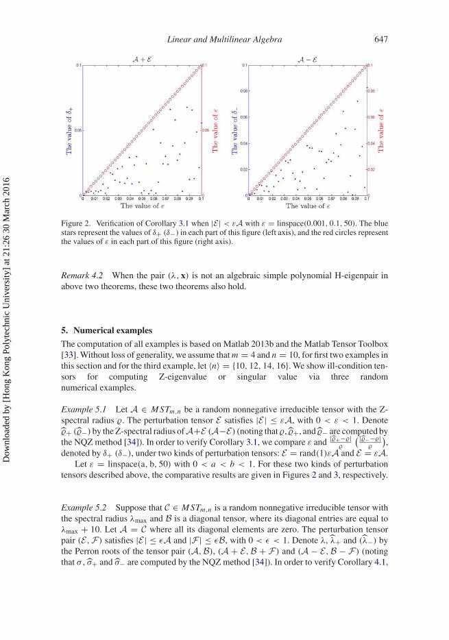
Figure 2. Verification of Corollary 3.1 when |E | < εA with ε = linspace(0.001, 0.1, 50). The bluestars represent the values of δ+ (δ−) in each part of this figure (left axis), and the red circles representthe values of ε in each part of this figure (right axis).
Remark 4.2 When the pair (λ, x) is not an algebraic simple polynomial H-eigenpair inabove two theorems, these two theorems also hold.
5. Numerical examples
The computation of all examples is based on Matlab 2013b and the Matlab Tensor Toolbox[33]. Without loss of generality, we assume that m = 4 and n = 10, for first two examples inthis section and for the third example, let 〈n〉 = {10, 12, 14, 16}. We show ill-condition ten-sors for computing Z-eigenvalue or singular value via three randomnumerical examples.
Example 5.1 Let A ∈ M STm,n be a random nonnegative irreducible tensor with the Z-spectral radius �. The perturbation tensor E satisfies |E | ≤ εA, with 0 < ε < 1. Denote�+ (�−) by the Z-spectral radius of A+E (A−E) (noting that �, �+, and �− are computed bythe NQZ method [34]). In order to verify Corollary 3.1, we compare ε and |�+−�|
�
( |�−−�|�
),
denoted by δ+ (δ−), under two kinds of perturbation tensors: E = rand(1)εA and E = εA.Let ε = linspace(a, b, 50) with 0 < a < b < 1. For these two kinds of perturbation
tensors described above, the comparative results are given in Figures 2 and 3, respectively.
Example 5.2 Suppose that C ∈ M STm,n is a random nonnegative irreducible tensor withthe spectral radius λmax and B is a diagonal tensor, where its diagonal entries are equal toλmax + 10. Let A = C where all its diagonal elements are zero. The perturbation tensorpair (E,F) satisfies |E | ≤ εA and |F | ≤ εB, with 0 < ε < 1. Denote λ, λ+ and (λ−) bythe Perron roots of the tensor pair (A,B), (A + E,B + F) and (A − E,B − F) (notingthat σ , σ+ and σ− are computed by the NQZ method [34]). In order to verify Corollary 4.1,
Dow
nloa
ded
by [
Hon
g K
ong
Poly
tech
nic
Uni
vers
ity]
at 2
1:26
30
Mar
ch 2
016
648 M. Che et al.
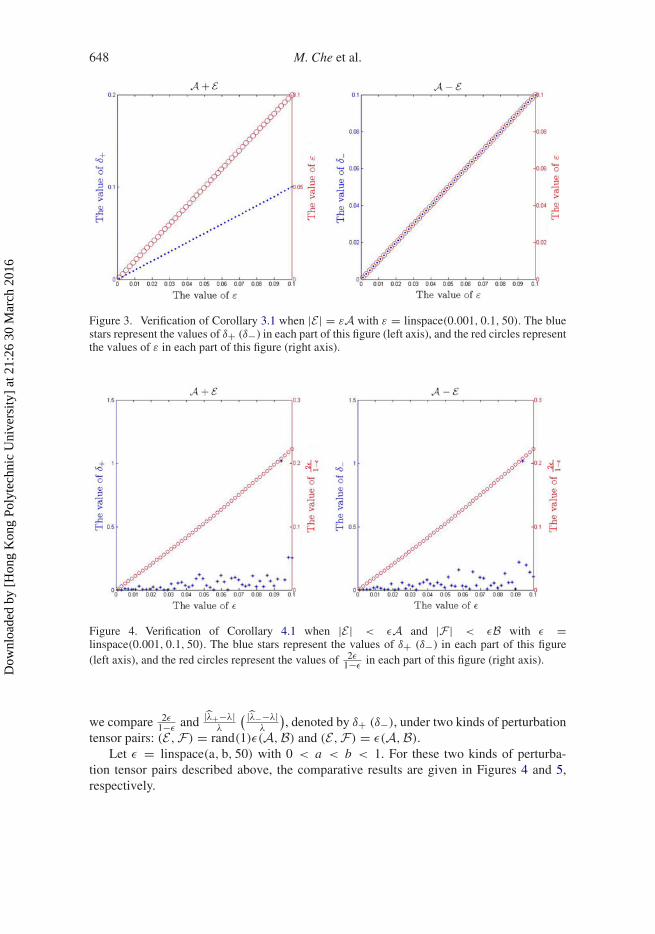
Figure 3. Verification of Corollary 3.1 when |E | = εA with ε = linspace(0.001, 0.1, 50). The bluestars represent the values of δ+ (δ−) in each part of this figure (left axis), and the red circles representthe values of ε in each part of this figure (right axis).
Figure 4. Verification of Corollary 4.1 when |E | < εA and |F | < εB with ε =linspace(0.001, 0.1, 50). The blue stars represent the values of δ+ (δ−) in each part of this figure(left axis), and the red circles represent the values of 2ε
1−εin each part of this figure (right axis).
we compare 2ε1−ε
and |λ+−λ|λ
( |λ−−λ|λ
), denoted by δ+ (δ−), under two kinds of perturbation
tensor pairs: (E,F) = rand(1)ε(A,B) and (E,F) = ε(A,B).Let ε = linspace(a, b, 50) with 0 < a < b < 1. For these two kinds of perturba-
tion tensor pairs described above, the comparative results are given in Figures 4 and 5,respectively.
Dow
nloa
ded
by [
Hon
g K
ong
Poly
tech
nic
Uni
vers
ity]
at 2
1:26
30
Mar
ch 2
016
Linear and Multilinear Algebra 649
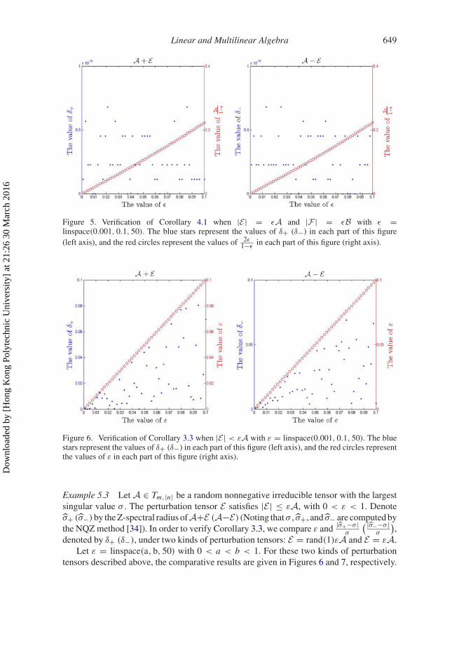
Figure 5. Verification of Corollary 4.1 when |E | = εA and |F | = εB with ε =linspace(0.001, 0.1, 50). The blue stars represent the values of δ+ (δ−) in each part of this figure(left axis), and the red circles represent the values of 2ε
1−εin each part of this figure (right axis).
Figure 6. Verification of Corollary 3.3 when |E | < εA with ε = linspace(0.001, 0.1, 50). The bluestars represent the values of δ+ (δ−) in each part of this figure (left axis), and the red circles representthe values of ε in each part of this figure (right axis).
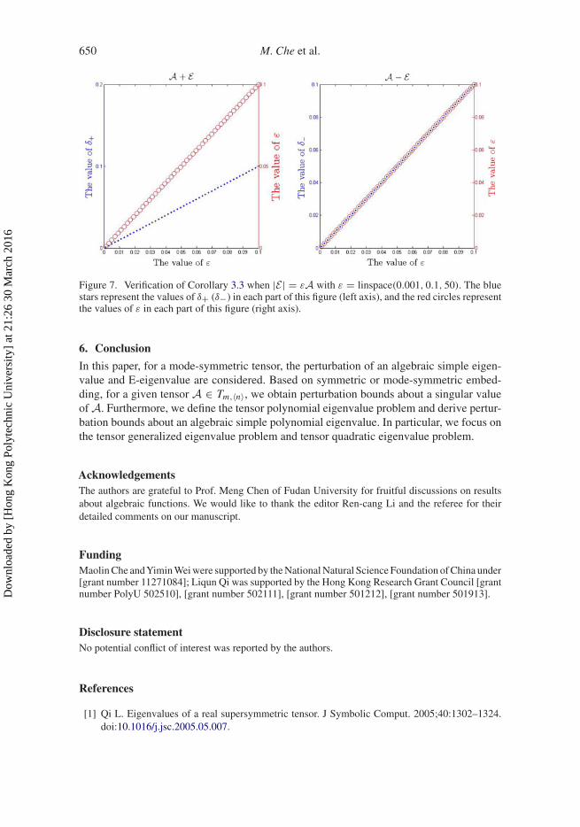
Example 5.3 Let A ∈ Tm,〈n〉 be a random nonnegative irreducible tensor with the largestsingular value σ . The perturbation tensor E satisfies |E | ≤ εA, with 0 < ε < 1. Denoteσ+ (σ−)by the Z-spectral radius ofA+E (A−E) (Noting thatσ , σ+, and σ− are computed bythe NQZ method [34]). In order to verify Corollary 3.3, we compare ε and |σ+−σ |
σ
( |σ−−σ |σ
),
denoted by δ+ (δ−), under two kinds of perturbation tensors: E = rand(1)εA and E = εA.Let ε = linspace(a, b, 50) with 0 < a < b < 1. For these two kinds of perturbation
tensors described above, the comparative results are given in Figures 6 and 7, respectively.
Dow
nloa
ded
by [
Hon
g K
ong
Poly
tech
nic
Uni
vers
ity]
at 2
1:26
30
Mar
ch 2
016
650 M. Che et al.
Figure 7. Verification of Corollary 3.3 when |E | = εA with ε = linspace(0.001, 0.1, 50). The bluestars represent the values of δ+ (δ−) in each part of this figure (left axis), and the red circles representthe values of ε in each part of this figure (right axis).
6. Conclusion
In this paper, for a mode-symmetric tensor, the perturbation of an algebraic simple eigen-value and E-eigenvalue are considered. Based on symmetric or mode-symmetric embed-ding, for a given tensor A ∈ Tm,〈n〉, we obtain perturbation bounds about a singular valueof A. Furthermore, we define the tensor polynomial eigenvalue problem and derive pertur-bation bounds about an algebraic simple polynomial eigenvalue. In particular, we focus onthe tensor generalized eigenvalue problem and tensor quadratic eigenvalue problem.
AcknowledgementsThe authors are grateful to Prof. Meng Chen of Fudan University for fruitful discussions on resultsabout algebraic functions. We would like to thank the editor Ren-cang Li and the referee for theirdetailed comments on our manuscript.
FundingMaolin Che andYimin Wei were supported by the National Natural Science Foundation of China under[grant number 11271084]; Liqun Qi was supported by the Hong Kong Research Grant Council [grantnumber PolyU 502510], [grant number 502111], [grant number 501212], [grant number 501913].
Disclosure statementNo potential conflict of interest was reported by the authors.
References
[1] Qi L. Eigenvalues of a real supersymmetric tensor. J Symbolic Comput. 2005;40:1302–1324.doi:10.1016/j.jsc.2005.05.007.
[2] Lim L. Singular values and eigenvalues of tensors: a variational approach. In: IEEE CAMSAP2005: First International Workshop on Computational Advances in Multi-Sensor AdaptiveProcessing. IEEE; 2005. p. 129–132.
[3] Golub GH, Van Loan CF. Matrix computations. 4th ed. Baltimore (MD): Johns Hopkins Studiesin the Mathematical Sciences, Johns Hopkins University Press; 2013.
[4] Chang KC, Pearson K, Zhang T. Perron–Frobenius theorem for nonnegative tensors. Commun.Math. Sci. 2008;6:507–520. http://projecteuclid.org/euclid.cms/1214949934.
[5] Chang KC, Pearson K, Zhang T. On eigenvalue problems of real symmetric tensors. J. Math.Anal. Appl. 2009;350:416–422. doi:10.1016/j.jmaa.2008.09.067.
[6] Kolda TG, Mayo JR. An adaptive shifted power method for computing generalized tensoreigenpairs. SIAM J. Matrix Anal. Appl. 2014;35:1563–1581. doi:10.1137/140951758.
[7] Cui CF, Dai YH, Nie J. All real eigenvalues of symmetric tensors. SIAM J. Matrix Anal. Appl.2014;35:1582–1601.
[8] Qi L, Wang Y, Wu EX. D-eigenvalues of diffusion kurtosis tensors. J. Comput. Appl. Math.2008;221:150–157. doi:10.1016/j.cam.2007.10.012.
[9] Ding W, Wei Y. Generalized tensor eigenvalue problems. SIAM J. Matrix Anal. Appl. 2015;36:1073–1099.
[10] Li W, Ng MK. The perturbation bound for the spectral radius of a nonnegative tensor. Adv.Numer. Anal. 2014:10 p. Article ID 109525. doi:10.1155/2014/109525.
[11] Li W, Ng MK. Some bounds for the spectral radius of nonnegative tensors. Numer. Math.2015;130:315–335.
[12] Cichocki A, Zdunek R, Phan AH, Amari Si. Nonnegative matrix and tensor factorizations:applications to exploratory multi-way data analysis and blind source separation. New York(NY): John Wiley & Sons; 2009.
[14] De Lathauwer L, De Moor B, Vandewalle J. A multilinear singular value decomposition. SIAMJ. Matrix Anal. Appl. 2000;21:1253–1278. doi:10.1137/S0895479896305696.
[15] Berman A, Plemmons RJ. Nonnegative matrices in the mathematical sciences. Vol. 9, Classics inapplied mathematics. Philadelphia (PA): Society for Industrial and Applied Mathematics; 1994.doi:10.1137/1.9781611971262.
[16] Chang KC, Qi L, Zhang T. A survey on the spectral theory of nonnegative tensors. Numer. LinearAlgebra Appl. 2013;20:891–912. doi:10.1002/nla.1902.
[17] Hu S, Huang ZH, Ling C, Qi L. On determinants and eigenvalue theory of tensors. J. SymbolicComput. 2013;50:508–531.
[18] Ding W, Qi L, Wei Y. M-tensors and nonsingular M-tensors. Linear Algebra Appl.2013;439:3264–3278.
[19] Zhang T. Existence of real eigenvalues of real tensors. Nonlinear Anal. 2011;74:2862–2868.doi:10.1016/j.na.2011.01.008.
[20] Wilkinson JH. The algebraic eigenvalue problem. New York (NY): Oxford University Press;1965.
[21] Demmel JW. Applied numerical linear algebra. Philadelphia (PA): Society for Industrial andApplied Mathematics (SIAM); 1997. doi:10.1137/1.9781611971446.
[22] Stewart GW, Sun JG. Matrix perturbation theory. Boston (MA): Computer Science and ScientificComputing, Academic Press Inc; 1990.
[23] Ragnarsson S, Van Loan CF. Block tensors and symmetric embeddings. Linear Algebra Appl.2013;438:853–874. doi:10.1016/j.laa.2011.04.014.
[24] Chen Z, Lu L. A tensor singular values and its symmetric embedding eigenvalues. J. Comput.Appl. Math. 2013;250:217–228. doi:10.1016/j.cam.2013.03.014.
[25] Cartwright D, Sturmfels B. The number of eigenvalues of a tensor. Linear Algebra Appl.2013;438:942–952. doi:10.1016/j.laa.2011.05.040.
[26] Kolda TG, Mayo JR. Shifted power method for computing tensor eigenpairs. SIAM J. MatrixAnal. Appl. 2011;32:1095–1124. doi:10.1137/100801482.
[27] Ahlfors LV. Complex analysis: an introduction of the theory of analytic functions of one complexvariable. 2nd ed. New York (NY): McGraw-Hill Book Co.; 1966.
[28] Chevalley C. Introduction to the theory of algebraic functions of one variable. No. VI.Mathematical surveys. New York (NY): American Mathematical Society; 1951.
[29] Gohberg I, Koltracht I. Mixed, componentwise, and structured condition numbers. SIAM J.Matrix Anal. Appl. 1993;14:688–704. doi:10.1137/0614049.
[30] Yang Y, Yang Q. Further results for Perron–Frobenius theorem for nonnegative tensors. SIAMJ. Matrix Anal. Appl. 2010;31:2517–2530.
[31] Elsner L, Koltracht I, Neumann M, Xiao D. On accurate computations of the Perron root. SIAMJ. Matrix Anal. Appl. 1993;14:456–467. doi:10.1137/0614032.
[32] Zhang T, Golub GH. Rank-one approximation to high order tensors. SIAM J. Matrix Anal. Appl.2001;23:534–550.
[33] Bader BW, Kolda TG. Matlab Tensor Toolbox Version 2.5. 2012 Jan. Available from: http://www.sandia.gov/tgkolda/TensorToolbox/.
[34] Ng M, Qi L, Zhou G. Finding the largest eigenvalue of a nonnegative tensor. SIAM J. MatrixAnal. Appl. 2009;31:1090–1099. doi:10.1137/09074838X.