Perturbation theory for the Stark effect in a double δ quantum well This article has been downloaded from IOPscience. Please scroll down to see the full text article. 2004 J. Phys. A: Math. Gen. 37 9735 (http://iopscience.iop.org/0305-4470/37/41/009) Download details: IP Address: 132.177.228.65 The article was downloaded on 21/02/2013 at 20:27 Please note that terms and conditions apply. View the table of contents for this issue, or go to the journal homepage for more Home Search Collections Journals About Contact us My IOPscience
Transcript
Perturbation theory for the Stark effect in a double δ quantum well
This article has been downloaded from IOPscience. Please scroll down to see the full text article.
2004 J. Phys. A: Math. Gen. 37 9735
(http://iopscience.iop.org/0305-4470/37/41/009)
Download details:
IP Address: 132.177.228.65
The article was downloaded on 21/02/2013 at 20:27
Please note that terms and conditions apply.
View the table of contents for this issue, or go to the journal homepage for more
Home Search Collections Journals About Contact us My IOPscience
INSTITUTE OF PHYSICS PUBLISHING JOURNAL OF PHYSICS A: MATHEMATICAL AND GENERAL
J. Phys. A: Math. Gen. 37 (2004) 9735–9748 PII: S0305-4470(04)81560-9
Perturbation theory for the Stark effect in a double δquantum well
Gabriel Alvarez1 and Bala Sundaram2
1 Departamento de Fısica Teorica II, Facultad de Ciencias Fısicas, Universidad Complutense,28040 Madrid, Spain2 Department of Mathematics and Graduate Faculty in Physics, CSI-CUNY, Staten Island,New York 10314, USA
Received 2 June 2004, in final form 1 September 2004Published 29 September 2004Online at stacks.iop.org/JPhysA/37/9735doi:10.1088/0305-4470/37/41/009
AbstractWe study the Stark effect in a symmetric double δ quantum well, for which thereare two kinds of resonances: the familiar resonances stemming from the boundstates, and a doubly infinite family of resonances stemming from the zero-fieldcontinuum threshold. We derive explicit expressions for the Borel-summableRayleigh–Schrodinger perturbation series for the resonances stemming fromthe bound states, for the imaginary part of these same resonances and for all theresonances stemming from the zero-field continuum threshold. The techniquesused in this paper are directly applicable to realistic models of quantum squarewell potentials with or without barriers.
PACS numbers: 32.60.+i, 31.15.Md, 02.30.Lt
1. Introduction
Besides its interest as a simple almost exactly solvable model in quantum mechanics [1, 2],the one-dimensional δ quantum well has attracted attention as a realistic model in severalphysical situations, usually in the context of photodetachment or photoionization in thepresence of electric fields. For example, it is well-known that in the presence of a staticelectric field the unique bound state of a δ potential well turns into a resonance and Elberfeldand Kleber [3] used this resonance as a model for tunnelling in ultrathin GaAs/GaxAl1−xAsquantum wells, deriving low and high-field asymptotic expansions for both its real part and itsimaginary part.
But already in 1987 Ludviksson [4] had shown that in addition to this well-knownresonance stemming from the bound state, there is a doubly infinite family of resonancesoriginating from the zero-field continuum threshold. In this same paper, Ludvikssonalso derived lowest-order asymptotic formulae for the positions of these resonances inthe complex energy plane as the applied electric field tends to zero. The role of these
resonances in photodetachment of H− by weak periodic fields has been discussed recentlyby Emmanouilidou and Reichl [5], who showed that the model reproduces several qualitativefeatures of the experimental cross section. Also very recently, Alvarez and Sundaram [6]discussed the systematic derivation of low and high-field asymptotic expansions for all theseresonances, and tracked them numerically as functions of the electric field, thus giving acomplete picture of their behaviour in the complex energy plane. Apparently unaware ofLudviksson’s paper, Cavalcanti, Giacconi and Soldati [7] have given an independent proof ofthe existence of the threshold resonances and, with due care of the required regularization,extended the results to two and three dimensions. We would like to mention also thatthe appearance of Stark resonances without bound-state predecessors in the local short-range Hulthen and Yukawa potentials has been studied numerically by Gonzalez-Ferez andSchweizer [8].
The double δ quantum well to which this paper is devoted was initially studied asa model for the hydrogen molecular ion H+
2. This model, although clearly less realistic,permits simplified treatments of typical double well phenomena as the exponentially smallsplitting between pairs of quasi-degenerate energy levels [9–13], and appears naturallyin dimensional perturbation theory [14]. From the scattering theory point of view[1, 2], the main difference between the single δ and the double δ quantum wells is theappearance in the latter of intrinsic (i.e. not induced by the external field) resonances.These resonances have been studied theoretically by Albeverio and Høegh-Krohn [15], whoused them as an example in their general perturbation theory for resonances, while theirphysical consequences were quantified by Alvarez and Silverstone [16], who derived an exactexpansion of the photoionization cross section of a particle in a double δ quantum well bya weak periodic field as a sum over these resonances plus a slowly varying backgroundterm.
Less studied, however, is the Stark effect in the double δ quantum well, despite an ongoinginterest in resonances induced by electric fields in quantum wells [17, 18]. The most relevantcontribution seems to be a recent paper by Korsch and Mossmann [19] in a different context:as we will show in the next section, there are two independent parameters in the correspondingHamiltonian, and Korsch and Mossmann use it as a convenient model to study the propertiesof resonance states as these parameters are varied. Concretely, they derive the condition forthe existence of resonances, demonstrate the existence of two types of crossing scenariosand investigate the resonance eigenfunctions for cyclic variations of the parameters wheregeometric phases can be observed. However, a systematic study of the Stark effect in thedouble δ quantum well, with a characterization of all the resonances and their behaviours asfunctions of the applied field seems to be lacking.
In this paper we present a complete discussion of the Stark effect in the double δ quantumwell from the point of view of perturbation theory. In section 2 we first quickly reviewthe field-free case in a form and with a notation suitable for later use, and then proceed toa straightforward derivation of the condition for the existence of resonances. Section 3 isdevoted to the resonances stemming from the bound states: we first show how to calculateexplicitly as many terms as desired of the Borel-summable Rayleigh–Schrodinger perturbationtheory power series (in which the imaginary part of the resonances appears implicitly in theprocess of Borel summation), and then we calculate an explicit asymptotic expansion for theexponentially small imaginary part of these resonances. In section 4 we study the two familiesof resonances stemming from the continuum threshold and show that they can be describedeither by an ‘exact’ Puiseux series or by an asymptotic expansion derived from it. Thepaper ends with a brief summary of the main ideas and of possible applications of the resultsherein.
Perturbation theory for the Stark effect in a double δ quantum well 9737
2. The Stark effect in a double δ quantum well
The time-independent Schrodinger equation for a particle of mass m and electric charge e ina double δ quantum well and an external uniform electric field Fc reads(
− h2
2m
d2
dx2c
− gc(δ(xc + a) + δ(xc − a)) − eFcxc
)�(xc) = Ec�(xc) (1)
where the subindex ‘c’ denotes conventional units and we take the distance between the wells2a > 0, the coupling constant gc > 0 (so that we have in fact wells and not barriers) and theapplied electric field Fc � 0.
By scaling the independent and dependent variables and the parameters in equation (1)according to
x = xc/a ψ(x) = �(xc) (2)
g = magc/h2 F = mea3Fc/h
2 E = ma2Ec/h2 (3)
we can transform the Schrodinger equation into the form(−1
2
d2
dx2− g(δ(x + 1) + δ(x − 1)) − Fx
)ψ(x) = Eψ(x) (4)
where g > 0 and F � 0. In this section we will first review the analytic structure of theunperturbed case F = 0 and then proceed to a straightforward derivation of the condition forthe existence of resonances in the perturbed case F > 0.
2.1. The unperturbed double δ well
Since the Schrodinger equation (4) with F = 0 is invariant under the parity transformationx → −x, we will look separately for its even and odd solutions. We write the even solutionsin the form
ψ(+)k (x) =
(1/2)[F+(k) eikx + F+(−k) e−ikx] x < −1
cos(kx) −1 � x � 1
(1/2)[F+(k) e−ikx + F+(−k) eikx] 1 < x
(5)
where
E = 12k2 (6)
and the Jost function F+(k) is determined by the continuity of the wavefunction at x = ±1and by the discontinuity of its derivative at the same points, which must be −2gψ(±1). Sincethe wavefunction (5) is even by construction, it is enough to require
ψ(+)k (1+) − ψ
(+)k (1−) = 0 (7)
ψ(+)′k (1+) − ψ
(+)′k (1−) = −2gψ
(+)k (1) (8)
from which follows immediately
F+(k) = 1 +ig
k(−e2ik − 1). (9)
Likewise, the odd solutions of equation (4) with F = 0 can be written in the form
ψ(−)k (x) =
(i/2)[F−(−k) e−ikx − F−(k) eikx] x < −1
sin(kx) −1 � x � 1
(i/2)[F−(k) e−ikx − F−(−k) eikx] 1 < x
(10)
9738 G Alvarez and B Sundaram
and by imposing the same matching conditions we find
F−(k) = 1 +ig
k(e2ik − 1). (11)
For later reference we point out that the even and odd Jost functions differ in just one sign,and can be written jointly as
F∓(k) = 1 +ig
k(±e2ik − 1). (12)
We also note that F−(k) and kF+(k) are entire functions of k and that
F∓(−k) = F∓(k). (13)
In particular, for k real the wavefunctions are real and∫ ∞
−∞ψ
(±)k (x)ψ
(±)k′ (x) dx = πF±(k)F±(−k)δ(k − k′). (14)
The bound states correspond to solutions of F±(k) = 0 of the form k = iκ with κ > 0,i.e. to the real positive solutions of the equations
κ
g− 1 = ±e−2κ . (15)
It is immediately verified that the double δ quantum well has exactly one even-parity boundstate and, if 2g > 1, exactly one odd-parity bound state. For large values of g the correspondingsolutions κ± of equation (15) have the asymptotic behaviours
κ± ∼ g ± g e−2g + · · · g → ∞ (16)
and as is typical of double-well potentials, the energy difference between the odd and evenbound states is exponentially small in the coupling constant g
�E = E− − E+ = 12
(κ2
+ − κ2−) ∼ 2g2 e−2g + · · · g → ∞. (17)
In addition there are infinitely many nonreal zeros of the even Jost function, all of them in thelower half k plane, and asymptotically given by
k+ = π
(n +
1
2
) [1 +
1
2g+
1
(2g)2+
1 − 43π2
(n + 1
2
)2
(2g)3+ · · ·
]
− iπ2
(n +
1
2
)2 [1
(2g)2+
3
(2g)3+ · · ·
]n = 0,±1,±2, . . . g → ∞
(18)
and infinitely many nonreal zeros of the odd Jost function, all of them in the lower half k plane,with asymptotic behaviours
k− = πn
[1 +
1
2g+
1
(2g)2+
1 − 43π2n2
(2g)3+ · · ·
]− iπ2n2
[1
(2g)2+
3
(2g)3+ · · ·
]n = ±1,±2, . . . g → ∞. (19)
Note that as a consequence of equation (13) these resonances can be grouped in pairs of theform k = ±Re (k) − i|Im (k)|. Some authors [1] apply the term resonance to all the zeros inequations (18) and (19), while others [2] reserve it for the zeros with Re k > 0 and Im k < 0.The first usage of the term is motivated by considering the resonances as (all) the poles of theresolvent in the lower half k plane; the second, by the fact that if |Im k| is sufficiently smalland the resonances are well-separated, each one may give a directly observable peak in, forexample, the photoionization cross section [16]. In any event, we want to stress that becausethey satisfy F±(k) = 0, equations (5) and (10) show that these latter intrinsic resonances withRe k > 0 correspond to purely outgoing waves in both directions of the real axis.
Perturbation theory for the Stark effect in a double δ quantum well 9739
2.2. The perturbed double δ well
Let us consider now the Schrodinger equation (4) with F > 0, which corresponds to apiecewise linear potential whose solutions can be written in terms of Airy functions [20]. Itis well-known from functional-analytic methods that the spectrum of the Stark operator isabsolutely continuous and fills the real line [21]. Since the linear potential tends to +∞ asx → −∞, there is only one bounded linearly independent solution of equation (4) for eachreal value of E. Equivalently, as x → −∞ we have to use the exponentially decreasing Airyfunction Ai(−(2F)1/3(x + E/F)), which has to be connected with linear combinations ofAi(−(2F)1/3(x + E/F)) and Bi(−(2F)1/3(x + E/F)) across the two centres x = ∓1 of theδ potentials.
However, anticipating the calculation of resonances, we will write the solution for 1 < x
directly in terms of the linear combinations of Ai(z) and Bi(z) with purely outgoing andincoming behaviour as z = −(2F)1/3(x + E/F) → −∞, for which we use the notation ofreference [22]:
Summing up, for given values of E and F > 0 we write the solution of equation (4) in theform
ψ(x) =
Ai(z(x)) x < −1
c(A) Ai(z(x)) + c(B) Bi(z(x)) −1 � x � 1
c(+) Ai(+)(z(x)) + c(−) Ai(−)(z(x)) 1 < x
(21)
where
z(x) = −(2F)1/3(x + E/F). (22)
By imposing the continuity of the wavefunction and the discontinuity of its derivativeat x = ∓1 we arrive at a set of four linear equations which are readily solved for the fourcoefficients c(A), c(B), c(+) and c(−) as functions of the energy E (the resulting expressions canbe greatly simplified using the Wronskian of the Airy functions W(Ai(z), Bi(z)) = 1/π ). Inthis perturbed case, the resonances correspond to purely outgoing waves as x → +∞ (andtherefore z(x) → −∞), i.e. to complex solutions of c(−)(E) = 0. This condition for theexistence of resonances can be conveniently written in terms of the following parameters
Equation (26) with a different scaling has been derived by the equivalent transfer-matrixformalism by Korsch and Mossmann [19], who used it for their numerical studies of thevariation of the resonances as the distance between the wells and the applied electric field arevaried. We devote the rest of the paper to a systematic analytic study of all the solutions ofthe resonance condition (26) from the point of view of perturbation theory, and to the ensuingrelation with the bound states and resonances of the unperturbed double well discussed at thebeginning of this section.
9740 G Alvarez and B Sundaram
3. Resonances stemming from the bound states
We devote this section to the resonances stemming from the bound states, where the particle,initially confined in the potential well, escapes towards x = +∞ by tunnelling, and we expectan exponentially small width. In other words, we look for solutions E(F) of the resonancecondition (26) that in the limit F → 0 tend to the unperturbed bound states E± < 0. Therefore,by equations (24) and (25), we have to study the solutions of equation (26) as z± → +∞. Themathematically rigorous and unambiguous way to solve equation (26) in this limit is to usethe concept of Borel summability [6, 23].
The Borel-summable asymptotic expansion for the Airy function Ai(z) in a sectorcontaining the positive real axis is discussed in [22, 23], in which it is shown that
Ai(z) ∼ 12π−1/2z−1/4e− 2
3 z3/2
2F0(
16 , 5
6 ; ;− 34z−3/2) |arg z| < 2
3π (27)
where
2F0(a, b; ; z) =∞∑
k=0
(a)k(b)kzk
k!(28)
is a generalized formal hypergeometric series and where (a)k is the Pochhammer symbol:(a)0 = 1, (a)k = a(a + 1) · · · (a + k − 1) for k > 0. Note in particular the sector of validity|arg z| < 2
3π , which is a proper subset of the sector of validity in the Poincare sense |arg z| < π
given in equation 10.4.59 of [20].However, the real positive axis is a Stokes line for the Borel-summable asymptotic
expansion of Bi(z) implicit in the definition of Ai(+)(z):
Bi(z) ∼ π−1/2z−1/4e23 z3/2
2F0(
16 , 5
6 ; ; 34z−3/2)
± i 12π−1/2z−1/4e− 2
3 z3/2
2F0(
16 , 5
6 ; ;− 34z−3/2
)0 < ± arg z < 2
3π. (29)
Again, see [22, 23] for the derivation of these Borel-summable expansions of the function Bi(z)with the ensuing unique determination of the exponentially small subseries, in contrast withthe asymptotic expansion in the Poincare sense given in equation 10.4.63 of [20]. Therefore,due to this Stokes line, the solution of equation (26) by asymptotic methods has to be carriedout independently on each side of the positive real axis.
3.1. The Borel-summable Rayleigh–Schrodinger power series
Let us consider first the upper side of the Stokes line Re F > 0, Im F > 0 and use the abridgednotation
�A(z) = z−1/42F0
(16 , 5
6 ; ;− 34z−3/2
)(30)
�B(z) = z−1/42F0
(16 , 5
6 ; ; 34z−3/2
)(31)
�AB(z) = �A(z)�B(z). (32)
By substituting equations (27) and (29) with the minus sign into equation (26) we arrive at theformally real asymptotic equation
1 = γ
2(�AB(z+) + �AB(z−)) +
γ 2
4
(e
43 (z
3/2+ −z
3/2− )�B(z+)
2�A(z−)2 − �AB(z+)�AB(z−)). (33)
Perturbation theory for the Stark effect in a double δ quantum well 9741
To calculate the expansion of the right-hand side of equation (33) we study first the factore
43 (z
3/2+ −z
3/2− ). By substituting the relation
E = − 12κ2 (34)
and the definitions (24) and (25) of z± into this exponential, we find that it can be expanded asa power series in F 2 whose coefficients are a global e−4κ factor times rational functions of κ:
e43 (z
3/2+ −z
3/2− ) = e−4κ
(1 +
2
3κ3F 2 +
4κ + 9
18κ7F 4 + · · ·
). (35)
Next we note that with the same substitutions for E and z±, the remaining terms in equation (33)can be readily expanded as a power series and therefore the right-hand side of equation (33)is in fact a power series in F 2. We absorb the 1 in the left-hand side into this power series anddenote it by Pr(κ), of which we show explicitly the first two terms to illustrate the pattern:
Pr(κ) =(
1 − κ
g
)2
− e−4κ +gF 2
4κ8
(5g − 5κ + 8gκ2 − 12κ3
− g e−4κ
(5 + 10κ + 8κ2 +
8
3κ3
))+ O(F 4). (36)
Therefore equation (33) can be written in the form
Pr(κ) = 0 (37)
and solved by writing κ itself as a Borel-summable power series in F 2
κ = κ(0)(F ) =∞∑
j=0
κ2jF2j . (38)
We substitute this expansion into equation (37) and recursively equate to zero the coefficientsof the powers of F. To order F 0 we find(
1 − κ0
g
)2
− e−4κ0 = F−(iκ0)F+(iκ0) = 0 (39)
where we have used the definitions (12) of F∓(k) and we see that in the limit F → 0we recover the conditions for the existence of the even and odd bound states (15). Usingequation (39) to eliminate e−4κ0 from higher perturbation coefficients we can generate the κ2j
as explicit rational functions of the coupling constant g and of the first coefficient κ0, whosetwo possible values are in turn determined by the equations for the existence of the unperturbedeven and odd bound states (39). By way of example,
κ2 = 15(κ0 − g) +(30 + 8κ2
0
)(κ0 − g)2 + 12κ2
0 (2κ0 − g)
24κ50 (κ0 − g)(2κ0 − 2g + 1)
(40)
and although κ4 is already too unwieldy to be calculated by hand, the procedure can be easilyprogrammed in a computer and the κ2j generated to high order.
In turn, the Borel-summable Rayleigh–Schrodinger perturbation theory series
E =∞∑
j=0
E2jF2j (41)
can be calculated immediately from equation (34), and since the coefficients E2j arepolynomials in the κ2j , the E2j inherit the structure of explicit rational functions of g andκ0. We want to stress that the formally real Rayleigh–Schrodinger power series (41) is Borel-summable to the exact resonances in the upper half plane Im F > 0, and that the imaginarypart of the resonances appears implicitly in the process of Borel summation [6].
9742 G Alvarez and B Sundaram
3.2. Asymptotic expansion for the imaginary part of the resonances
Although the formally real Rayleigh–Schodinger power series (41) encodes both the exactreal part and the exact imaginary part of the resonances stemming from the bound states, it isdesirable to have an explicit asymptotic expansion for the imaginary part of the resonances. Toachieve this goal, we solve equation (26) at the lower side of the Stokes line, i.e. we considernow Re F > 0, Im F < 0. By substituting equations (27) and (29) with the plus sign intoequation (26) we arrive at the explicitly complex asymptotic equation
1 = γ
2
[�AB(z+) + �AB(z−) + i
(e− 4
3 z3/2+ �A(z+)
2 + e− 43 z
3/2− �A(z−)2)]
+γ 2
4
[e
43 (z
3/2+ −z
3/2− )�B(z+)
2�A(z−)2 − �AB(z+)�AB(z−)
+ i(e− 4
3 z3/2− �AB(z+)�A(z−)2 − e− 4
3 z3/2+ �A(z+)
2�AB(z−))]
(42)
which can be written in the form
Pr(κ) + i e−2κ3/(3F)Pi(κ) = 0 (43)
where Pr(κ) has been defined in equation (36) and Pi(κ) is a power series in F whose firsttwo terms are
Pi(κ) = 2g
κ
(g
κsinh(2κ) − cosh(2κ)
)+
gF
6κ5((5κ + 12κ3) cosh(2κ)
− (5g + 12κ2 + 12gκ2) sinh(2κ)) + O(F 2). (44)
Because of the exponentially small factor that multiplies Pi(κ) in equation (43), its Borel-summable solution is indeed the same power series (38) plus a sequence of successivelyexponentially smaller subseries, alternately formally real and formally imaginary, which wewrite in the form
κ = κ(0)(F ) + κ(1)(F ) + κ(2)(F ) + · · · . (45)
The exponentially small corrections κ(p)(F ) with p � 1 can be calculated from the alreadyknown κ(0)(F ) by a Taylor expansion. For example, the first exponentially small correction is
κ(1)(F ) = −i e−2κ(0)(F )3/(3F) Pi(κ(0)(F ))
P ′r (κ
(0)(F ))(46)
where the prime denotes the derivative of Pr(κ) with respect to its argument κ .At this point note that both asymptotic expansions (38) and (45) represent the same
analytic (and therefore continuous) function κ(F ) on adjacent sectors. In particular
κ(F − i0) = κ(F + i0) (47)
while in the Borel-sum sense
κ(0)(F − i0) = κ(0)(F + i0). (48)
As a consequence we have the following explicit, Borel-summable asymptotic expansion forthe imaginary part
i Im [κ(F + i0)] = 12 (κ(1)(F − i0) + κ(2)(F − i0) + · · ·) (49)
where we have used the notation F ± i0 as a reminder of the sectors in which each term isvalid. Equations (34), (38), (46) and (49) lead to the corresponding asymptotic expansion forthe imaginary part of the resonance energy
Perturbation theory for the Stark effect in a double δ quantum well 9743
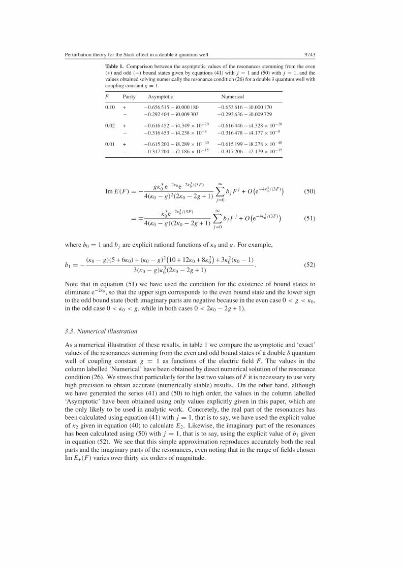
Table 1. Comparison between the asymptotic values of the resonances stemming from the even(+) and odd (−) bound states given by equations (41) with j = 1 and (50) with j = 1, and thevalues obtained solving numerically the resonance condition (26) for a double δ quantum well withcoupling constant g = 1.
Note that in equation (51) we have used the condition for the existence of bound states toeliminate e−2κ0 , so that the upper sign corresponds to the even bound state and the lower signto the odd bound state (both imaginary parts are negative because in the even case 0 < g < κ0,in the odd case 0 < κ0 < g, while in both cases 0 < 2κ0 − 2g + 1).
3.3. Numerical illustration
As a numerical illustration of these results, in table 1 we compare the asymptotic and ‘exact’values of the resonances stemming from the even and odd bound states of a double δ quantumwell of coupling constant g = 1 as functions of the electric field F. The values in thecolumn labelled ‘Numerical’ have been obtained by direct numerical solution of the resonancecondition (26). We stress that particularly for the last two values of F it is necessary to use veryhigh precision to obtain accurate (numerically stable) results. On the other hand, althoughwe have generated the series (41) and (50) to high order, the values in the column labelled‘Asymptotic’ have been obtained using only values explicitly given in this paper, which arethe only likely to be used in analytic work. Concretely, the real part of the resonances hasbeen calculated using equation (41) with j = 1, that is to say, we have used the explicit valueof κ2 given in equation (40) to calculate E2. Likewise, the imaginary part of the resonanceshas been calculated using (50) with j = 1, that is to say, using the explicit value of b1 givenin equation (52). We see that this simple approximation reproduces accurately both the realparts and the imaginary parts of the resonances, even noting that in the range of fields chosenIm E+(F ) varies over thirty six orders of magnitude.
9744 G Alvarez and B Sundaram
4. Resonances stemming from the continuum threshold
The resonances stemming from the even and odd bound states studied in the previous sectionare not the only solutions of the resonance condition (26). We have to consider also thesolutions in which as F → 0, both z+ and z− simultaneously tend either to a zero of Ai(z) orto a zero of Ai(+)(z). These resonances are analogous to the resonances induced by an electricfield in a single δ quantum well first described by Ludviksson [4] and subsequently studied byseveral authors as we discussed in the introduction [5–7, 19]. Note that from the definitionsof z± in equations (24) and (25) it follows that
E = − z±21/3
F 2/3 ∓ F (53)
and therefore these resonant energies E tends to 0 (the continuum threshold) as F 2/3.
4.1. Solutions of Ai(z) = 0
The zeros as of the Airy function Ai(z) are located on the negative real axis, and can be labelledby a positive integer s. From the asymptotic expansion of the Airy Ai(z) function for negativevalues of the argument (equation 10.4.60 in [20]) it is easy to derive asymptotic expansions forthe zeros (equation 10.4.94 in [20]), expansions which are increasingly accurate as s → ∞.For our purposes it is sufficient to consider the leading term
as ∼ −[
3π
8(4s − 1)
]2/3
s = 1, 2, . . . . (54)
We will use also the following equations
Ai′(as) ∼ (−1)s−1
π1/2
[3π
8(4s − 1)
]1/6
(55)
Bi(as) ∼ (−1)s
π1/2
[3π
8(4s − 1)
]−1/6
(56)
Bi′(as) ∼ (−1)s
4π1/2
[3π
8(4s − 1)
]−5/6
(57)
which are obtained from the corresponding asymptotic expansions for the Airy functions Ai(z)and Bi(z) and the trivial result Ai′′(as) = as Ai(as) = 0.
4.2. Resonances that tend to solutions of Ai(z) = 0 as F → 0
In order to find the behaviour of these resonances as F → 0 we solve the resonance condition(26) by using a Puiseux expansion of the solution (namely, a power series in F 1/3). Althoughthe expansion can be carried out without difficulty to high order, we show explicitly only thefirst three terms because, as we will see later, the third term is the lowest term necessary forthe imaginary part of the resonance to enter the solution. Therefore we write
Perturbation theory for the Stark effect in a double δ quantum well 9745
Substituting the Taylor expansions (59) for z± into equation (26) and using the asymptoticformulas (54)–(57) we find
Es(F ) ∼ F 2/3
21/3
[3π
8(4s − 1)
]2/3
+ F
(1 +
1
4g+
1
4g − 2
)
+F 4/3
(4g)2(1 − 2g)2
[2 − i3π(4s − 1)]
[6π(4s − 1)]2/3+ O(F 5/3) s = 1, 2, . . . . (61)
Although this asymptotic formula for the first kind of threshold resonances is increasinglyaccurate as s → ∞ (i.e. for higher resonances), numerical tests show that it gives accurateresults for any value of s. Equation (61) shows that indeed the imaginary part of the resonanceenters in the third term of the expansion, and that
Im (Es) ∼ − [Re (Es)]2
g2(1 − 2g)23π(4s − 1)F → 0. (62)
Therefore infinitely many resonances approach the origin from the fourth quadrant along afamily of increasingly flatter parabolas. This fact explains the sensitivity of a direct numericalsolution of equation (26) to initial data in a neighbourhood of the origin. Equation (61)provides the means to identify and track down the results of these numerical calculations.
4.3. Resonances that tend to solutions of Ai(+)(z) = 0 as F → 0
The expressions for the second kind of threshold resonances, which correspond to solutionsof the resonance condition (26) in which z± tend to a zero of Ai(+)(z), can be almost read offfrom the expansions by drawing on equation (20). Indeed, if we set
z± = w± e−2π i/3 (63)
the resonance condition (26) can be written in the form
Equation (65) describes the second kind of threshold resonances, all of which approach theorigin along the ray arg(Es) = −2π/3 in the third quadrant as F → 0.
4.4. Numerical illustration
These results are illustrated by a numerical example in table 2, where we compare theasymptotic, ‘Puiseux’ and numerical values of the resonances E1(F ) and E1(F ) for the samevalues of the electric field F used in table 1. The values in the column labelled ‘Asymptotic’have been obtained with the explicit equations (61) and (65) with s = 1, while the valuesin the column labelled ‘Numerical’ have been calculated by direct numerical solution of theresonance condition (26). As we mentioned earlier, the main problem of a numerical solutionin this case is to give a sufficiently accurate initial approximation to the desired root. In
9746 G Alvarez and B Sundaram
Table 2. Comparison among the asymptotic, Puiseux and numerical values of the first (s = 1)
resonance of each kind stemming from the continuum threshold for a double δ quantum well withcoupling constant g = 1. The asymptotic values have been obtained with equations (61) and (65);the Puiseux values, with five exact terms of the series (58) and the numerical values by directnumerical solution of the resonance condition (26).
fact, in the calculations displayed in table 2 we have used the asymptotic values as initialapproximations for the numerical solution. The main difference with respect to table 1 is thatnow the asymptotic values do not tend to the exact ones as F → 0, because in the derivation ofequations (61) and (65) we have not used the exact values as for the zeros of the Airy function,but their approximate values (54) which are increasingly accurate as s → ∞ (therefore, theexample shows the worst possible case). To illustrate this fact we have included in the tablethe column labelled ‘Puiseux’ which has been calculated using five ‘exact’ terms of the series(58) where by ‘exact’ we mean that accurate numerical values of the zeros as , of Bi(as) and ofthe derivatives Ai′(as) and Bi′(as) have been used to calculate the coefficients instead of theasymptotic formulae (54)–(57). Note that from the physical point of view these resonancesare much wider than the resonances stemming from the bound states and that their main effectin the photoionization cross section will be to contribute to the background by raising thebaseline before the threshold and to increase the asymmetry of the peaks [5, 16, 24].
4.5. Final remarks on the existence of resonances
Finally, let us consider the asymptotic expansion for large k of the resonance condition (26)in the sector Re k > 0, −π/3 < Im k < 0 which contains the first family of thresholdresonances (61). This asymptotic expansion can be easily derived from the fundamentalasymptotic expansions (27) and (29) and the ‘relations between solutions’ of the Airydifferential equation given in equations 10.4.6–10.4.9 of [20]. The full expansion has theform Q1(k) + ei2k3/(3F)Q2(k) = 0, where Q1(k) and Q2(k) are power series in F 2 and Frespectively, but for the purposes of these final remarks it will be enough to show the leadingterms of each series:[(
1 − ig
k
)2−
( ig
ke2ik
)2+ O(F 2)
]+ ei2k3/(3F)
[2g2
k2sin(2k) − 2g
kcos(2k) + O(F)
]= 0.
(66)
The leading term of Q1(k) is readily identified with F+(k)F−(k) (whose zeros are the intrinsicresonances of the unperturbed problem), but note that this is now the subdominant contribution.The presence of the dominant exponential and the corresponding leading term of Q2(k) showsthat there are not solutions of equation (66) that in the limit F → 0 tend to k = kr − iki withki > 0 in the given sector. Incidentally, the leading term of Q2(k) is also easy to identify: if
Perturbation theory for the Stark effect in a double δ quantum well 9747
instead of looking for the even and odd solutions of the unperturbed double δ well we look forthe solution that represents for x < −1 a pure plane wave moving to the right
ψ(r)k (x) = F−(−k)ψ
(+)k (x) + iF+(−k)ψ
(−)k (x) (67)
or more explicitly
ψ(r)k (x) =
eikx x < −1
(1 + ig/k) eikx − (ig/k) e−2ik e−ikx −1 � x � 1
ρ(k) e−ikx + σ(k) eikx 1 < x
(68)
where
ρ(k) = 1
2[F+(k)F−(−k) − F+(−k)F−(k)] = 2ig2
k2sin(2k) − 2ig
kcos(2k) (69)
σ(k) = F+(−k)F−(−k) =(
1 +ig
k
)2−
( ig
ke−2ik
)2(70)
we see that the leading term of Q2(k) is (minus i times) the coefficient ρ(k), and that itsreal zeros correspond to the k values for which there is maximum transmission (i.e. no wavemoving to the left in the region 1 < x) in the unperturbed double δ well. Furthermore, notethat asymptotically these real values of k are given by
k = nπ
2
[1 +
1
2g+
1
(2g)2+
1 − 43 (nπ/2)2
(2g)3+ · · ·
]g → ∞ (71)
and are asymptotically equal to the real parts of both the even and odd resonances inequations (18) and (19).
5. Summary
In this paper we have studied the Stark effect in the double δ quantum well from the pointof view of perturbation theory. We have shown that there are two kinds of resonances: thefamiliar resonances stemming from the bound states and a doubly infinite family of resonancesstemming from the continuum threshold. These resonances were first described by Ludviksson[4] in the simpler context of the single δ quantum well and there is also numerical evidence oftheir existence in short range potentials [8].
We have derived explicit expressions for the coefficients of the Borel-summable Rayleigh–Schrodinger perturbation theory series for the resonances stemming from the bound states, aswell as explicit asymptotic expansions for the imaginary part of these resonances. The keyidea for an efficient derivation of these results is to use in effect perturbation theory not onthe resonance energy directly but on the wavenumber. Likewise, we have derived asymptoticexpansions for both kinds of resonances stemming from the unperturbed continuum threshold.These expansions show that resonances of the first kind approach the origin from the fourthquadrant along increasingly flatter parabolas, while resonances of the second kind approachthe origin along the ray arg E = −2π/3 in the third quadrant. Moreover, while the width ofthe resonances stemming from the bound states is exponentially small in F, the width of thethreshold resonances of the first kind of threshold resonances behaves as F 4/3 while the widthof the second kind behaves as F 2/3 when F → 0.
But beyond the concrete results pertaining to the double δ model we would like to stressthe applicability of the method in a situation which, albeit slightly more complicated fromthe computational point of view, has direct physical interest: the extraction of electrons by
9748 G Alvarez and B Sundaram
an electric field in (effectively one-dimensional) quantum wells [17, 18]. Since these wellsare usually modelled by square well potentials without or with barriers [24], the solutionof the corresponding Stark problem reduces again to the matching of Airy wavefunctions inpiecewise linear potentials, which leads to an explicit condition for the existence of resonancesanalogous to our equation (26), to which the techniques developed in this paper can be directlyapplied. In particular, we consider of special interest the calculation of the photoionizationcross section of a realistic GaAs/GaxAl1−xAs well by the method of [24] but in the presenceof an applied electric field.
Acknowledgment
The work of GA was supported by Spanish Ministerio de Ciencia y Tecnologıa grantBFM2002-02646. The work of BS was supported by US National Science Foundation grantno 0099431.
References
[1] Alveberio S, Gesztesy F, Høegh-Krohn R and Holden H 1988 Solvable Models in Quantum Mechanics (NewYork: Springer)
[2] Galindo A and Pascual P 1990 Quantum Mechanics I (New York: Springer)[3] Elberfeld W and Kleber M 1988 Z. Phys. B 73 23[4] Ludviksson A 1987 J. Phys. A: Math. Gen. 20 4733[5] Emmanouilidou A and Reichl L E 2000 Phys. Rev. A 62 022709[6] Alvarez G and Sundaram B 2003 Phys. Rev. A 68 013407[7] Cavalcanti R M, Giacconi P and Soldati R 2003 J. Phys. A: Math. Gen. 36 12065[8] Gonzalez-Ferez R and Schweizer W 2001 Phys. Rev. A 64 033404[9] Frost A A 1956 J. Chem. Phys. 25 1150
[10] Robinson P D 1961 Proc. R. Soc. 78 537[11] Claverie P 1969 Int. J. Quantum Chem. 3 349[12] Certain P R and Byers Brown W 1972 Int. J. Quantum Chem. 6 131[13] Ahlrichs R and Claverie P 1972 Int. J. Quantum Chem. 6 1001[14] Huang S-W, Goodson D Z, Lopez-Cabrera M and Germann T C 1998 Phys. Rev. A 58 250[15] Alveberio S and Høegh-Krohn R 1984 J. Math. Anal. Appl. 101 491[16] Alvarez G and Silverstone H J 1989 Phys. Rev. A 40 3690[17] Kuo D M-T and Chang Y-C 1999 Phys. Rev. B 60 15957[18] Zambrano M L and Arce J C 2002 Phys. Rev. B 66 155340[19] Korsh H J and Mossmann S 2003 J. Phys. A: Math. Gen. 36 2139[20] Abramowitz M and Stegun I 1972 Handbook of Mathematical Functions (New York: Dover)[21] Sahbani J 2000 J. Math. Phys. 41 8006[22] Silverstone H J, Harris J G, Cızek J and Paldus J 1985 Phys. Rev. A 32 1965[23] Silverstone H J, Nakai S and Harris J G 1985 Phys. Rev. A 32 1341[24] Alvarez G and Luna E 2001 Phys. Rev. B 64 115303