Journal of Machine Learning Research 14 (2013) 2857-2898 Submitted 1/13; Revised 7/13; Published 9/13 Perturbative Corrections for Approximate Inference in Gaussian Latent Variable Models Manfred Opper OPPERM@CS. TU- BERLIN. DE Department of Computer Science Technische Universit¨ at Berlin D-10587 Berlin, Germany Ulrich Paquet ULRIPA@MICROSOFT. COM Microsoft Research Cambridge Cambridge CB1 2FB, United Kingdom Ole Winther OWI @IMM. DTU. DK Informatics and Mathematical Modelling Technical University of Denmark DK-2800 Lyngby, Denmark Editor: Neil Lawrence Abstract Expectation Propagation (EP) provides a framework for approximate inference. When the model under consideration is over a latent Gaussian field, with the approximation being Gaussian, we show how these approximations can systematically be corrected. A perturbative expansion is made of the exact but intractable correction, and can be applied to the model’s partition function and other moments of interest. The correction is expressed over the higher-order cumulants which are neglected by EP’s local matching of moments. Through the expansion, we see that EP is correct to first order. By considering higher orders, corrections of increasing polynomial complexity can be applied to the approximation. The second order provides a correction in quadratic time, which we apply to an array of Gaussian process and Ising models. The corrections generalize to arbitrarily complex approximating families, which we illustrate on tree-structured Ising model approxima- tions. Furthermore, they provide a polynomial-time assessment of the approximation error. We also provide both theoretical and practical insights on the exactness of the EP solution. Keywords: expectation consistent inference, expectation propagation, perturbation correction, Wick expansions, Ising model, Gaussian process 1. Introduction Expectation Propagation (EP) (Opper and Winther, 2000; Minka, 2001a,b) is part of a rich family of variational methods, which approximate the sums and integrals required for exact probabilistic inference by an optimization problem. Variational methods are perfectly amenable to probabilistic graphical models, as the nature of the optimization problem often allows it to be distributed across a graph. By relying on local computations on a graph, inference in very large probabilistic models becomes feasible. Being an approximation, some error may invariably be introduced. This paper is specifically concerned with the error that arises when a Gaussian approximating family is used, and lays a systematic foundation for examining and correcting these errors. It follows on earlier work by the c 2013 Manfred Opper, Ulrich Paquet and Ole Winther.
Transcript
Journal of Machine Learning Research 14 (2013) 2857-2898 Submitted 1/13; Revised 7/13; Published 9/13
Perturbative Corrections for Approximate Inference in Gaussian
authors (Opper et al., 2009). The error that arises when the free energy (the negative logarithm
of the partition function or normalizer of the distribution) is approximated, may for instance be
written as a Taylor expansion (Opper et al., 2009; Paquet et al., 2009). A pleasing property of EP
is that, at its stationary point, the first order term of such an expansion is zero. Furthermore, the
quality of the approximation can then be ascertained in polynomial time by including corrections
beyond the first order, or beyond the standard EP solution. In general, the corrections improve the
approximation when they are comparatively small, but can also leave a question mark on the quality
of approximation when the lower-order terms are large.
The approach outlined here is by no means unique in correcting the approximation, as is evinced
by cluster-based expansions (Paquet et al., 2009), marginal corrections for EP (Cseke and Heskes,
2011) and the Laplace approximation (Rue et al., 2009), and corrections to Loopy Belief Propaga-
tion (Chertkov and Chernyak, 2006; Sudderth et al., 2008; Welling et al., 2012).
1.1 Overview
EP is introduced in a general way in Section 3, making it clear how various degrees of complexity
can be included in its approximating structure. The partition function will be used throughout the
paper to explain the necessary machinery for correcting any moments of interest. In the experi-
ments, corrections to the marginal and predictive means and variances are also shown, although the
technical details for correcting moments beyond the partition function are relegated to Appendix D.
The Ising model, which is cast as a Gaussian latent variable model in Section 2, will furthermore be
used as a running example throughout the paper.
The key to obtaining a correction lies in isolating the “intractable quantity” from the “tractable
part” (or EP solution) in the true problem. This is done by considering the cumulants of both: as EP
locally matches lower-order cumulants like means and variances, the “intractable part” exists as an
expression over the higher-order cumulants which are neglected by EP. This process is outlined in
Section 4, which concludes with two useful results: a shift of the “intractable part” to be an average
over complex Gaussian variables with zero diagonal relation matrix, and Wick’s theorem, which
allows us to evaluate the expectations of polynomials under centered Gaussian measures. As a last
stage, the “intractable part” is expanded in Sections 5 and 7 to obtain corrections to various orders.
In Section 6, we provide a theoretical analysis of the radius of convergence of these expansions.
Experimental evidence is presented in Section 8 on Gaussian process (GP) classification and
(non-Gaussian) GP regression models. An insightful counterexample where EP diverges under
increasing data, is also presented. Ising models are examined in Section 9.
Numerous additional examples, derivations, and material are provided in the appendices. Details
on different EP approximations can be found in Appendix A, while corrections to tree-structured
approximations are provided in Appendix B. In Appendix C we analytically show that the correction
to a tractable example is zero. The main body of the paper deals with corrections to the partition
function, while corrections to marginal moments are left to Appendix D. Finally, useful calculations
of certain cumulants appear in Appendix E.
2. Gaussian Latent Variable Models
Let x = (x1, . . . ,xN) be an unobserved random variable with an intractable distribution p(x). In the
Gaussian latent variable model (GLVM) considered in this paper, terms tn(xn) are combined over a
2858
PERTURBATIVE CORRECTIONS FOR APPROXIMATE INFERENCE
quadratic exponential f0(x) to give
p(x) =1
Z
N
∏n=1
tn(xn) f0(x) (1)
with partition function (normalizer)
Z =∫ N
∏n=1
tn(xn) f0(x)dx .
This model encapsulates many important methods used in statistical inference. As an example, f0
can encode the covariance matrix of a Gaussian process (GP) prior on latent function observations
xn. In the case of GP classification with a class label yn ∈ {−1,+1} on a latent function evaluation
xn, the terms are typically probit link functions, for example
p(x) =1
Z
N
∏n=1
Φ(ynxn)N (x ; 0, K) . (2)
The probit function is the standard cumulative Gaussian density Φ(x) =∫ x−∞ N (z;0,1)dz. In this
example, the partition function is not analytically tractable but for the one-dimensional case N = 1.
An Ising model can be constructed by letting the terms tn restrict xn to ±1 (through Dirac delta
functions). By introducing the symmetric coupling matrix J and field θ into f0, an Ising model can
be written as
p(x) =1
Z
N
∏n=1
[1
2δ(xn +1)+
1
2δ(xn −1)
]
exp
{1
2xT Jx+θT x
}
. (3)
In the Ising model, the partition function Z is intractable, as it sums f0(x) over 2N binary values
of x. In the variational approaches, the intractability is addressed by allowing approximations to Z
and other marginal distributions, decreasing the computational complexity from being exponential
to polynomial in N, which is typically cubic for EP.
3. Expectation Propagation
An approximation to Z can be made by allowing p(x) in Equation (1) to factorize into a product
of factors fa. This factorization is not unique, and the structure of the factorization of p(x) defines
the complexity of the resulting approximation, resulting in different structures in the approximating
distribution. Where GLVMs are concerned, a natural and computationally convenient choice is
to use Gaussian factors ga, and as such, the approximating distribution q(x) in this paper will be
Gaussian. Appendix A summarizes a number of factorizations for Gaussian approximations.
The tractability of the resulting inference method imposes a pragmatic constraint on the choice
of factorization; in the extreme case p(x) could be chosen as a single factor and inference would
be exact. For the model in Equation (1), a three-term product may be factorized as (t1)(t2)(t3),which gives the typical GP setup. When a division is introduced and the term product factorizes
as (t1t2)(t2t3)/(t2), the resulting free energy will be that of the tree-structured EC approximation
(Opper and Winther, 2005). To therefore allow for regrouping, combining, splitting, and dividing
terms, a power Da is associated with each fa, such that
p(x) =1
Z∏
a
fa(x)Da (4)
2859
OPPER, PAQUET AND WINTHER
with intractable normalization (or partition function) Z =∫
∏a fa(x)Da dx.1 Appendix A shows
how the introduction of Da lends itself to a clear definition of tree-structured and more complex
approximations.
To define an approximation to p, terms ga, which typically take an exponential family form, are
chosen such that
q(x) =1
Zq∏
a
ga(x)Da (5)
has the same structure as p’s factorization. Although not shown explicitly, fa and ga have a depen-
dence on the same subset of variables xa. The optimal parameters of the ga-term approximations
are found through a set of auxiliary tilted distributions, defined by
qa(x) =1
Za
(q(x) fa(x)
ga(x)
)
. (6)
Here a single approximating term ga is replaced by an original term fa. Assuming that this replace-
ment leaves qa still tractable, the parameters in ga are determined by the condition that q(x) and
all qa(x) should be made as similar as possible. This is usually achieved by requiring that these
distributions share a set of generalised moments which usually coincide with the sufficient statistics
of the exponential family. For example with sufficient statistics φ(x) we require that
〈φ(x)〉qa= 〈φ(x)〉q for all a . (7)
Note that those factors fa in p(x) which are already in the exponential family, such as the Gaussian
terms in examples above, can trivially be solved for by setting ga = fa. The partition function
associated with this approximation is
ZEP = Zq ∏a
ZDaa . (8)
Appendix A.2 shows that the moment-matching conditions must hold at a stationary point of logZEP.
The EP algorithm iteratively updates the ga-terms by enforcing q to share moments with each of
the tilted distributions qa; on reaching a fixed point all moments match according to Equation (7)
(Minka, 2001a,b). Although ZEP is defined in the terminology of EP, other algorithms may be
required to solve for the fixed point, and ZEP, as a free energy, can be derived from the saddle point
of a set of self-consistent (moment-matching) equations (Opper and Winther, 2005; van Gerven
et al., 2010; Seeger and Nickisch, 2010). We next make EP concrete by applying it to the Ising
model, which will serve as a running example in the paper. The section is finally concluded with a
discussion of the interpretation of EP.
3.1 EP for Ising Models
The Ising model in Equation (3) will be used as a running example throughout this paper. To make
the technical developments more concrete, we will consider both the N-variate and bivariate cases.
The bivariate case can be solved analytically, and thus allows for a direct comparison to be made
between the exact and approximate solutions.
We use the factorized approximation as a running example, dividing p(x) in Equation (3) into
N + 1 factors with f0(x) = exp{ 12xT Jx+θT x} and fn(xn) = tn(xn) =
12δ(xn + 1)+ 1
2δ(xn − 1), for
1. The factorization and EP energy function is expressed here in the form of Power EP (Minka, 2004).
2860
PERTURBATIVE CORRECTIONS FOR APPROXIMATE INFERENCE
n = 1, . . . ,N (see Appendix A for generalizations). We consider the Gaussian exponential family
such that gn(xn) = exp{λn1xn − 12λn2x2
n} and g0(x) = f0(x). The approximating distribution from
Equation (5), q(x) ∝ f0(x)∏Nn=1 gn(xn), is thus a full multivariate Gaussian density, which we write
as q(x) = N (x;µ,Σ).
3.1.1 MOMENT MATCHING
The moment matching condition in Equation (7) involves only the mean and variance if q(x) fully
factorizes according to p(x)’s terms. We therefore only need to match the mean and variances of
marginals of q(x) and the tilted distribution qn(x) in Equation (6). The tilted distribution may be
decomposed into a Gaussian and a discrete part as qn(x) = qn(x\n|xn)qn(xn), where the vector x\n
consists of all variables apart from xn. We may marginalize out x\n and write qn(xn) in terms of two
factors:
qn(xn) ∝1
2
[
δ(xn +1)+δ(xn −1)]
︸ ︷︷ ︸
fn(x)=tn(xn)
exp{
γxn − 12Λx2
n
}
︸ ︷︷ ︸
∝∫
dx\n q(x)/gn(x)
, (9)
where we dropped the dependency of γ and Λ on n for notational simplicity. Through some manip-
ulation, the tilted distribution is equivalent to
qn(xn) =1+mn
2δ(xn −1)+
1−mn
2δ(xn +1) , mn = tanh(γ) =
eγ − e−γ
eγ + e−γ. (10)
This discrete distribution has mean mn and variance 1−m2n. By adapting the parameters of gn(xn)
using for example the EP algorithm, we aim to match the mean and variance of the marginal q(xn)(of q(x)) to the mean and variance of qn(xn). The reader is referred to Section 9 for benchmarked
results for the Ising model.
3.1.2 ANALYTIC BIVARIATE CASE
Here we shall compare the exact result with EP and the correction for the simplest non-trivial model,
the N = 2 Ising model with no external field
p(x) =1
4
(
δ(x1 −1)+δ(x1 +1))(
δ(x2 −1)+δ(x2 +1))
eJx1x2 .
In order to solve the moment matching conditions we observe that the mean values must be zero
because the distribution is symmetric around zero. Likewise the linear term in the approximat-
ing factors disappears and we can write gn(xn) = exp{−λx2n/2} and q(x) = N (x;0,Σ) with Σ =
[λ −J
−J λ
]−1
. The moment matching condition for the variances, 1 = Σnn, turns into a second
order equation with solution λ = 12
[
J2 +√
J4 +4]
. We can now insert this solution into the expres-
sion for the EP partition function in Equation (8). By expanding the result to the second order in J2,
we find that
logZEP =−1
2+
1
2
√
1+4J2 − 1
2log
(1
2(1+
√
1+4J2)
)
=J2
2− J4
4+ . . . .
Comparing with the exact expression
logZ = logcosh(J) =J2
2− J4
12+ . . .
2861
OPPER, PAQUET AND WINTHER
we see that EP gives the correct J2 coefficient, but the J4 coefficient comes out wrong. In Section 4
we investigate how cumulant corrections can correct for this discrepancy.
3.2 Two Explanations Why Gaussian EP is Often Very Accurate
EP, as introduced above, is an algorithm. The justification for the algorithm put forward by Minka
and adopted by others (see for example recent textbooks by Bishop 2006, Barber 2012 and Murphy
2012) is useful for explaining the steps in the algorithm but may be misleading in order to explain
why EP often provides excellent accuracy in estimation of marginal moments and Z.
The general justification for EP (Minka, 2001a,b) is based upon a minimization of Kullback-
Leiber (KL) divergences. Ideally, one would determine the approximating distribution q(x) as the
minimizer of KL(p‖q) in an exponential family of (in our case, Gaussian) densities. Since this
is not possible—it would require the computation of exact moments—we instead iteratively min-
imize “local” KL-divergences KL(qa‖q), between the tilted distribution qa and q, with respect to
ga (appearing in q). This leads to the moment matching conditions in Equation (7). The argument
for this procedure is essentially that this will ensure that the approximation q will capture high
density regions of the intractable posterior p. Obviously, this argument cannot be applied to Ising
models because the exact and approximate distributions are very different, with the former being
discrete due to the Dirac δ-functions that constrain xn = ±1 to be binary variables. Even though
the optimization still implies moment matching, this discrete-continuous discrepancy makes local
KL-divergences KL(qa‖q) infinite!
In order to justify the usefulness of EP for Ising models we therefore need an alternative argu-
ment. Our argument is entirely restricted to Gaussian EP for our extended definition of GLVMs and
do not extend to approximations with other exponential families. In the following, we will discuss
these assumptions in inference approximations that preceded the formulation of EP, in order to pro-
vide a possibly more relevant justification of the method. Although this justification is not strictly
necessary for practically using EP nor corrections to EP, it nevertheless provides a good starting
point for understanding both.
The argument goes back to the mathematical analysis of the Sherrington-Kirkpatrick (SK)
model for a disordered magnet (a so-called spin glass) (Sherrington and Kirckpatrick, 1975). For
this Ising model, the couplings J are drawn at random from a Gaussian distribution. An impor-
tant contribution in the context of inference for this model (the computations of partition functions
and average magnetizations) was the work of Thouless et al. (1977) who derived self-consistency
equations which are assumed to be valid with a probability (with respect to the drawing of ran-
dom couplings) approaching one as the number of variables xn grows to infinity. These so-called
Thouless-Anderson-Palmer (TAP) equations are closely related to the EP moment matching condi-
tions of Equation (7), but they differ by partly relying on the specific assumption of the randomness
of the couplings. Self-consistency equations equivalent to the EP moment matching conditions
which avoided such assumptions on the statistics of the random couplings were first derived by
Opper and Winther (2000) by using a so-called cavity argument (Mezard et al., 1987). A new im-
portant contribution of Minka (2001a) was to provide an efficient algorithmic recipe for solving
these equations.
We will now sketch the main idea of the cavity argument for the GLVM. Let x\n (“x without
n”) denote the complement to xn, that is x = x\n ∪ xn. Without loss of generality we will take the
quadratic exponential term to be written as f0(x) ∝ exp(−xT Jx/2). With similar definitions of J\n,
2862
PERTURBATIVE CORRECTIONS FOR APPROXIMATE INFERENCE
the exact marginal distribution of xn may be written as
pn(xn) =1
Ztn(xn)
∫exp
{
−1
2xT Jx
}
∏n′ 6=n
tn′(xn′)dx\n
=tn(xn)
Ze−Jnn x2
n/2
∫exp
{
−xn ∑n′ 6=n
Jnn′xn′ −1
2xT\nJ\nx\n
}
∏n′ 6=n
tn′(xn′)dx\n .
It is clear that pn(xn) depends entirely on the statistics of the random variable hn ≡∑n′ 6=n Jnn′xn′ . This
is the total ‘field’ created by all other ‘magnetic moments’ xn′ in the ‘cavity’ opened once xn has
been removed from the system. In the context of densely connected models with weak couplings,
we can appeal to the central limit theorem2 to approximate hn by a Gaussian random variable with
mean γn and variance Vn. When looking at the influence of the remaining variables x\n on xn, the
non-Gaussian details of their distribution have been washed out in the marginalization. Integrating
out the Gaussian random variable hn gives the Gaussian cavity field approximation to the marginal
distribution:
pn(xn)≈ const · tn(xn)e−Jnn x2n/2
∫e−xnh N (h ; γn,Vn)dh
= const · tn(xn)exp
{
−xnγn −1
2(Jnn −Vn)x
2n
}
.
This is precisely of the form of the marginal tilted distribution qn(xn) of Equation (9) as given by
Gaussian EP. In the cavity formulation, q(x) is simply a placeholder for the sufficient statistics of
the individual Gaussian cavity fields. So we may observe cases, with the Ising model or bounded
support factors being the prime examples, where EP gives essentially correct results for the marginal
distributions of the xn and of the partition function Z, while q(x) gives a poor or even meaningless
(in the sense of KL divergences) approximation to the multivariate posterior. Note however, that
the entire covariance matrix of the xn can be computed simply from a derivative of the free energy
(Opper and Winther, 2005) resulting in an approximation of this covariance by that of q(x). This
may indicate that a good EP approximation of the free energy may also result in a good approxi-
mation to the full covariance. The near exactness of EP (as compared to exhaustive summation) in
Section 9 therefore shows the central limit theorem at work. Conversely, mediocre accuracy or even
failure of Gaussian EP, as also observed in our simulations in Sections 8.3 and 9, may be attributed
to breakdown of the Gaussian cavity field assumption. Exact inference on the strongest couplings as
considered for the Ising model in Section 9 is one way to alleviate the shortcoming of the Gaussian
cavity field assumption.
4. Corrections to EP
The ZEP approximation can be corrected in a principled approach, which traces the following out-
line:
1. The exact partition function Z is re-written in terms of ZEP, scaled by a correction factor
R = Z/ZEP. This correction factor R encapsulates the intractability in the model, and contains
a “local marginal” contribution by each fa (see Section 4.1).
2. In the context of sparsely connected models, other cavity arguments lead to loopy belief propagation.
2863
OPPER, PAQUET AND WINTHER
2. A “handle” on R is obtained by writing it in terms of the cumulants (to be defined in Section
4.2) of q(x) and qa(x) from Equations (5) and (6). As qa(x) and q(x) share their two first
cumulants, the mean and covariance from the moment matching condition in Equation (7), a
cumulant expansion of R will be in terms of higher-order cumulants (see Section 4.2).
3. R, defined in terms of cumulant differences, is written as a complex Gaussian average. Each
factor fa contributes a complex random variable ka in this average (see Section 4.3).
4. Finally, the cumulant differences are used as “small quantities” in a Taylor series expansion
of R, and the leading terms are kept (see Sections 5 and 7).
The series expansion is in terms of a complex expectation with a zero “self-relation” matrix,
and this has two important consequences. Firstly, it causes all first order terms in the Taylor
expansion to disappear, showing that ZEP is correct to first order. Secondly, due to Wick’s
theorem (introduced in Section 4.4), these zeros will contract the expansion by making many
other terms vanish.
The strategy that is presented here can be re-used to correct other quantities of interest, like marginal
distributions or the predictive density of new data when p(x) is a Bayesian probabilistic model.
These corrections are outlined in Appendix D.
4.1 Exact Expression for Correction
We define the (intractable) correction R as Z = RZEP. We can derive a useful expression for R in a
few steps as follows: First we solve for fa in Equation (6), and substitute this into Equation (4) to
obtain
∏a
fa(x)Da = ∏
a
(Zaqa(x)ga(x)
q(x)
)Da
= ZEP q(x)∏a
(qa(x)
q(x)
)Da
. (11)
We introduce F(x)
F(x)≡ ∏a
(qa(x)
q(x)
)Da
to derive the expression for the correction R = Z/ZEP by integrating Equation (11):
R =∫
q(x)F(x)dx , (12)
where we have used Z =∫
∏a fa(x)Da dx. Similarly we can write:
p(x) =1
Z∏
a
fa(x)Da =
ZEP
Zq(x)F(x) =
1
Rq(x)F(x) . (13)
Corrections to the marginal and predictive densities of p(x) can be computed from this formulation.
This expression will become especially useful because the terms in F(x) turn out to be “local”, that
is, they only depend on the marginals of the variables associated with factor a. Let fa(x) depend
on the subset xa of x, and let x\a (“x without a”) denote the remaining variables. The distributions
in Equations (5) and (6) differ only with respect to their marginals on xa, qa(xa) and q(xa), and
thereforeqa(x)
q(x)=
q(x\a|xa)qa(xa)
q(x\a|xa)q(xa)=
qa(xa)
q(xa).
2864
PERTURBATIVE CORRECTIONS FOR APPROXIMATE INFERENCE
Now we can rewrite F(x) in terms of marginals:
F(x) = ∏a
(qa(xa)
q(xa)
)Da
. (14)
The key quantity, then, is F , after which the key operation is to compute its expected value. The
rest of this section is devoted to the task of obtaining a “handle” on F .
4.2 Characteristic Functions and Cumulants
The distributions present in each of the ratios in F(x) in Equation (14) share their first two cumu-
lants, mean and covariance. Cumulants and cumulant differences are formally defined in the next
paragraph. This simple observation has a crucial consequence: As the q(xa)’s are Gaussian and do
not contain any higher order cumulants (three and above), F can be expressed in terms of the higher
cumulants of the marginals qa(xa). When the term-product approximation is fully factorized, these
are simply cumulants of one-dimensional distributions.
Let Na be the number of variables in subvector xa. In the examples presented in this work, Na is
one or two. Furthermore, let ka be an Na-dimensional vector ka = (k1, . . . ,kNa)a. The characteristic
function of qa is
χa(ka) =∫
eikTa xa qa(xa)dxa =
⟨eikT
a xa⟩
qa, (15)
and is obtained through the Fourier transform of the density. Inversely,
qa(xa) =1
(2π)Na
∫e−ikT
a xaχa(ka)dka . (16)
The cumulants cαa of qa are the coefficients that appear in the Taylor expansion of logχa(ka) around
the zero vector,
cαa =
[
(−i)l
(∂
∂ka
)α
logχa(ka)
]
ka=0
.
By this definition of cαa, the Taylor expansion of logχa(ka) is
logχa(ka) =∞
∑l=1
il ∑|α|=l
cαa
α!kα
a .
Some notation was introduced in the above two equations to facilitate manipulating a multivariate
series. The vector α = (α1, . . . ,αNa), with α j ∈ N0, denotes a multi-index on the elements of ka.
Other notational conventions that employ α (writing k j instead of ka j) are:
|α|= ∑j
α j , kαa = ∏
j
kα j
j , α! = ∏j
α j! ,
(∂
∂ka
)α
= ∏j
∂α j
∂kα j
j
.
For example, when Na = 2, say for the edge-factors in a spanning tree, the set of multi-indices α
where |α|= 3 are (3,0), (2,1), (1,2), and (0,3).
There are two characteristic functions that come into play in F(x) and R in Equation (13). The
first is that of the tilted distribution, logχa(ka), and the other is the characteristic function of the
2865
OPPER, PAQUET AND WINTHER
EP marginal q(xa), defined as χ(ka) = 〈eikTa xa〉q. By virtue of matching the first two moments, and
q(xa) being Gaussian with cumulants c′αa,
ra(ka) = logχa(ka)− logχ(ka) = ∑l≥1
il ∑|α|=l
cαa − c′αa
α!kα
a
= ∑l≥3
il ∑|α|=l
cαa
α!kα
a (17)
contains the remaining higher-order cumulants where the tilted and approximate distributions differ.
All our subsequent derivations rest upon moment matching being attained. This especially means
that one cannot use the derived corrections if EP has not converged.
4.2.1 ISING MODEL EXAMPLE
The cumulant expansion for the discrete distribution in Equation (10) becomes
logχn(kn) = log
∫dxn eiknxnqn(xn) = log
(1+m
2eikn +
1−m
2e−ikn
)
= imkn −1
2!(1−m2)k2
n −i
3!(−2m+2m3)k3
n +1
4!(−2+8m2 −6m4)k4
n + · · ·
(we’re compactly writing m for mn), from which the cumulants are obtained as
c1n = m , c4n =−2+8m2 −6m4 ,
c2n = 1−m2 , c5n = 16m−40m3 +24m5 ,
c3n =−2m+2m3 , c6n = 16−136m2 +240m4 −120m6 .
4.3 The Correction as a Complex Expectation
The expected value of F , which is required for the correction, has a dependence on a product of
ratios of distributions qa(xa)/q(xa). In the preceding section it was shown that the contributing
distributions share lower-order statistics, allowing a twofold simplification. Firstly, the ratio qa/q
will be written as a single quantity that depends on ra, which was introduced above in Equation (17).
Secondly, we will show that it is natural to shift integration variables into the complex plane, and
rely on complex Gaussian random variables (meaning that both real and imaginary parts are jointly
Gaussian). These complex random variables that define the ra’s have a peculiar property: they have
a zero self-relation matrix! This property has important consequences in the resulting expansion.
4.3.1 COMPLEX EXPECTATIONS
Assume that q(xa) = N (xa ; µa,Σa) and qa(xa) share the same mean and covariance, and substitute
logχa(ka) = ra(ka)+ logχ(ka) in the definition of qa in Equation (16) to give
qa(xa)
q(xa)=
∫e−ikT
a xa+ra(ka) χ(ka)dka∫e−ikT
a xa χ(ka)dka
. (18)
Although the ka variables have not been introduced as random variables, we find it natural to in-
terpret them as such, because the rules of expectations over Gaussian random variables will be
2866
PERTURBATIVE CORRECTIONS FOR APPROXIMATE INFERENCE
−10
1−1 0 1 2 3 4
−1
−0.5
0
0.5
1
Re(k)x
Im(k
)
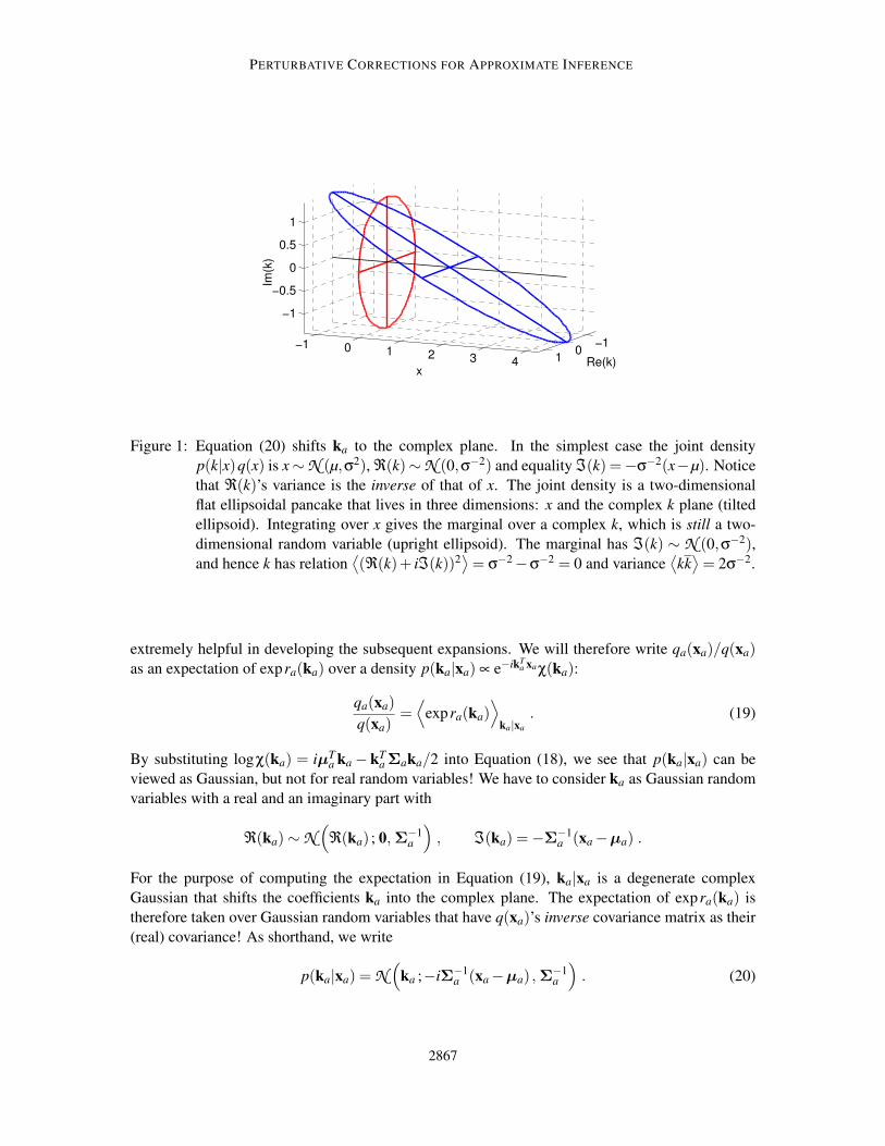
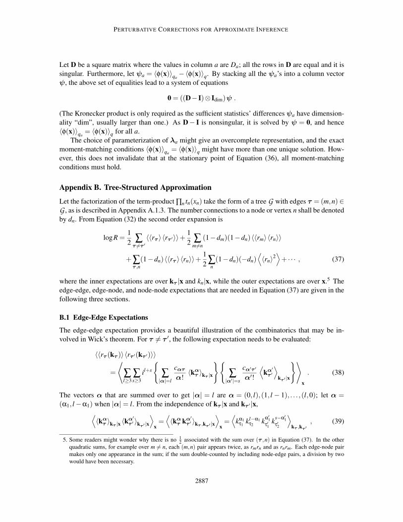
Figure 1: Equation (20) shifts ka to the complex plane. In the simplest case the joint density
p(k|x)q(x) is x ∼ N (µ,σ2), ℜ(k)∼ N (0,σ−2) and equality ℑ(k) =−σ−2(x−µ). Notice
that ℜ(k)’s variance is the inverse of that of x. The joint density is a two-dimensional
flat ellipsoidal pancake that lives in three dimensions: x and the complex k plane (tilted
ellipsoid). Integrating over x gives the marginal over a complex k, which is still a two-
dimensional random variable (upright ellipsoid). The marginal has ℑ(k) ∼ N (0,σ−2),and hence k has relation
⟨(ℜ(k)+ iℑ(k))2
⟩= σ−2 −σ−2 = 0 and variance
⟨kk⟩= 2σ−2.
extremely helpful in developing the subsequent expansions. We will therefore write qa(xa)/q(xa)as an expectation of expra(ka) over a density p(ka|xa) ∝ e−ikT
a xaχ(ka):
qa(xa)
q(xa)=⟨
expra(ka)⟩
ka|xa
. (19)
By substituting logχ(ka) = iµTa ka − kT
a Σaka/2 into Equation (18), we see that p(ka|xa) can be
viewed as Gaussian, but not for real random variables! We have to consider ka as Gaussian random
variables with a real and an imaginary part with
ℜ(ka)∼ N(
ℜ(ka) ; 0,Σ−1a
)
, ℑ(ka) =−Σ−1a (xa −µa) .
For the purpose of computing the expectation in Equation (19), ka|xa is a degenerate complex
Gaussian that shifts the coefficients ka into the complex plane. The expectation of expra(ka) is
therefore taken over Gaussian random variables that have q(xa)’s inverse covariance matrix as their
(real) covariance! As shorthand, we write
p(ka|xa) = N(
ka ;−iΣ−1a (xa −µa) ,Σ
−1a
)
. (20)
2867
OPPER, PAQUET AND WINTHER
Figure 1 illustrates a simple density p(ka|xa), showing that the imaginary component is a de-
terministic function of xa. Once xa is averaged out of the joint density p(ka|xa)q(xa), a circularly
symmetric complex Gaussian distribution over ka remains. It is circularly symmetric as 〈ka〉= 0, re-
lation matrix⟨kakT
a
⟩= 0, and covariance matrix
⟨kaka
T⟩= 2Σ−1
a (notation k indicates the complex
conjugate of k). For the purpose of computing the expected values with Wick’s theorem (following
in Section 4.4 below), we only need the relations⟨kakT
b
⟩for pairs of factors a and b. All of these
will be derived next:
According to Equation (12), a further expectation over q(x) is needed, after integrating over
ka, to determine R. These variables will be combined into complex random variables to make the
averages in the expectation easier to derive. By substituting Equation (19) into Equation (12), R is
equal to
R =⟨F(x)
⟩
x∼q(x)=
⟨
∏a
⟨
expra(ka)⟩Da
ka|xa
⟩
x
. (21)
When x is given, the ka-variables are independent. However, when they are averaged over q(x), the
ka-variables become coupled. They are zero-mean complex Gaussians
〈ka〉=⟨
〈ka〉ka|xa
⟩
x=⟨
−iΣ−1a (xa −µa)
⟩
x= 0
and are coupled with a zero self-relation matrix! In other words, if Σab = cov(xa,xb), the expected
values⟨kakT
b
⟩between the variables in the set {ka} are
⟨kakT
b
⟩=⟨⟨
kakTb
⟩
ka,b|x
⟩
x+ i2Σ−1
a
⟨
(xa −µa)(xb −µb)T⟩
xΣ
−1b
=
{0 if a = b
−Σ−1a ΣabΣ
−1b if a 6= b
. (22)
Complex Gaussian random variables are additionally characterized by⟨kakb
T⟩. However, these
expectations are not required for computing and simplifying the expansion of logR in Section 5,
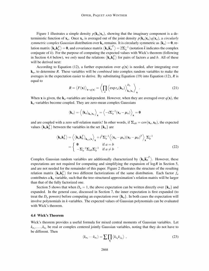
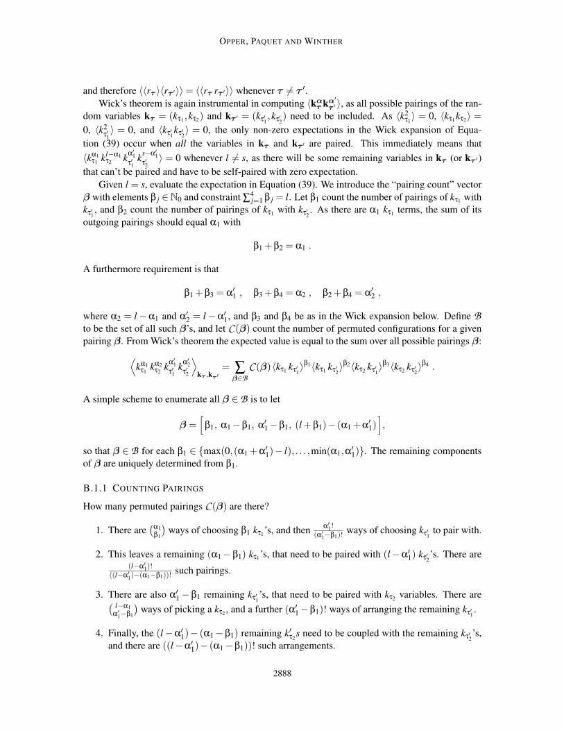
and are not needed for the remainder of this paper. Figure 2 illustrates the structure of the resulting
relation matrix⟨kakT
b
⟩for two different factorizations of the same distribution. Each factor fa
contributes a ka variable, such that the tree-structured approximation’s relation matrix will be larger
than that of the fully factorized one.
Section 5 shows that when Da = 1, the above expectation can be written directly over {ka} and
expanded. In the general case, discussed in Section 7, the inner expectation is first expanded (to
treat the Da powers) before computing an expectation over {ka}. In both cases the expectation will
involve polynomials in k-variables. The expected values of Gaussian polynomials can be evaluated
with Wick’s theorem.
4.4 Wick’s Theorem
Wick’s theorem provides a useful formula for mixed central moments of Gaussian variables. Let
kn1, . . . ,knℓ be real or complex centered jointly Gaussian variables, noting that they do not have to
be different. Then
〈kn1· · ·knℓ〉= ∑∏
η
⟨kiηk jη
⟩, (23)
2868
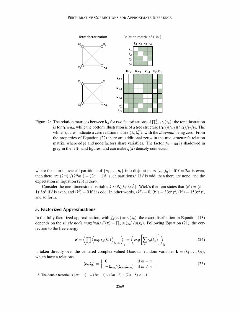
PERTURBATIVE CORRECTIONS FOR APPROXIMATE INFERENCE
Figure 2: The relation matrices between ka for two factorizations of ∏4n=1 tn(xn): the top illustration
is for t1t2t3t4, while the bottom illustration is of a tree structure (t1t2)(t2t3)(t3t4)/t2/t3. The
white squares indicate a zero relation matrix⟨kakT
b
⟩, with the diagonal being zero. From
the properties of Equation (22) there are additional zeros in the tree structure’s relation
matrix, where edge and node factors share variables. The factor f0 = g0 is shadowed in
grey in the left-hand figures, and can make q(x) densely connected.
where the sum is over all partitions of {n1, . . . ,nℓ} into disjoint pairs {iη, jη}. If ℓ = 2m is even,
then there are (2m)!/(2mm!) = (2m−1)!! such partitions.3 If ℓ is odd, then there are none, and the
expectation in Equation (23) is zero.
Consider the one-dimensional variable k ∼ N (k;0,σ2). Wick’s theorem states that 〈kℓ〉= (ℓ−1)!!σℓ if ℓ is even, and 〈kℓ〉= 0 if ℓ is odd. In other words, 〈k3〉= 0, 〈k4〉= 3(σ2)2, 〈k6〉= 15(σ2)3,
and so forth.
5. Factorized Approximations
In the fully factorized approximation, with fn(xn) = tn(xn), the exact distribution in Equation (13)
depends on the single node marginals F(x) = ∏n qn(xn)/q(xn). Following Equation (21), the cor-
rection to the free energy
R =
⟨
∏n
⟨
exprn(kn)⟩
kn|xn
⟩
x
=
⟨
exp
[
∑n
rn(kn)
]⟩
k
(24)
is taken directly over the centered complex-valued Gaussian random variables k = (k1, . . . ,kN),which have a relations
〈kmkn〉={
0 if m = n
−Σmn/(ΣmmΣnn) if m 6= n. (25)
3. The double factorial is (2m−1)!! = (2m−1)× (2m−3)× (2m−5)×·· ·1.
2869
OPPER, PAQUET AND WINTHER
In the section to follow, all expectations shall be with respect to k, which will be dropped where it
is clear from the context.
Thus far, R is re-expressed in terms of site contributions. The expression in Equation (24) is
exact, albeit still intractable, and will be treated through a power series expansion. Other quantities
of interest, like marginal distributions or moments, can similarly be expressed exactly, and then
expanded (see Appendix D).
5.1 Second Order Correction to logR
Assuming that the rn’s are small on average with respect to k, Equation (24) is expanded and the
lower order terms kept:
logR = log
⟨
exp
[
∑n
rn(kn)
]⟩
= ∑n
〈rn〉+1
2
⟨(
∑n
rn
)2⟩
− 1
2
(
∑n
〈rn〉)2
+ · · ·
=1
2∑
m6=n
〈rmrn〉+ · · · (26)
The simplification in the second line is a result of the variance terms being zero from Equation (25).
The single marginal terms also vanish (and hence EP is correct to first order) because both 〈kn〉= 0
and⟨k2
n
⟩= 0.
This result can give us a hint in which situations the corrections are expected to be small:
• Firstly, the rn could be small for values of kn where the density of k is not small. For example,
under a zero noise Gaussian process classification model, qn(xn) equals a step function tn(xn)times a Gaussian, where the latter often has small variance compared to the mean. Hence,
qn(xn) should be very close to a Gaussian.
• Secondly, for systems with weakly (posterior) dependent variables xn we might expect that
the log partition function logZ would scale approximately linearly with N, the number of
variables. Since terms with m = n vanish in the computation of lnR, there are no corrections
that are proportional to N when Σmn is sufficiently small as N → ∞. Hence, the dominant
contributions to logZ should already be included in the EP approximation. However, Section
8.3 illustrates an example where this need not be the case.
The expectation 〈rmrn〉, as it appears in Equation (26), is treated by substituting rn with its cumulant
expansion rn(kn) = ∑l≥3 ilclnkln/l! from Equation (17). Wick’s theorem now plays a pivotal role in
evaluating the expectations that appear in the expansion:
〈rm(km)rn(kn)〉= ∑l,s≥3
il+s cln csm
l!s!〈ks
mkln〉
= ∑l≥3
i2ll!cln csm
(l!)2〈kmkn〉l
= ∑l≥3
clm cln
l!
(Σmn
ΣmmΣnn
)l
. (27)
The second line above follows from contractions in Wick’s theorem. All the self-pairing terms,
when for example one of the l kn’s is paired with another kn in Equation (23), are zero because
2870
PERTURBATIVE CORRECTIONS FOR APPROXIMATE INFERENCE
⟨k2
n
⟩= 0. To therefore get a non-zero result for
⟨ks
mkln
⟩, using Equation (23), each factor kn has to
be paired with some factor km, and this is possible only when l = s. Wick’s theorem sums over all
pairings, and there are l! ways of pairing a kn with a km, giving the result in Equation (27). Finally,
plugging Equation (27) into Equation (26) gives the second order correction
logR =1
2∑
m6=n
∑l≥3
clm cln
l!
(Σmn
ΣmmΣnn
)l
+ · · · . (28)
5.1.1 ISING EXAMPLE CONTINUED
We can now compute the second order logR correction for the N = 2 Ising model example of
Section 3.1. The covariance matrix has Σnn = 1 from moment matching and Σ12 = J/(λ2 − J2)
with λ = 12
[
J2 +√
J4 +4]
. The uneven terms in the cumulant expansion derived in Section 4.2.1
disappear because m = 0. The first nontrivial term is therefore l = 4 which gives a contribution of12× 2× c2
4
4!Σ4
12 = (−2)2
4!Σ4
12 = 16Σ4
12. In Section 3.1, we saw that logZ − logZEP = J4
6plus terms of
order J6 and higher. To lowest order in J we have Σ12 = J and thus logR = J4
6which exactly cancels
the lowest order error of EP.
5.2 Corrections to Other Quantities
The schema given here is applicable to any other quantity of interest, be it marginal or predictive
distributions, or the marginal moments of p(x). The cumulant corrections for the marginal moments
are derived in Appendix D; for example, the correction to the marginal mean µi of an approximation
q(x) = N (x;µ,Σ) is
〈xi〉p(x)−µi = ∑l≥3
∑j 6=n
Σi j
Σ j j
cl+1, jcln
l!
(Σ jn
Σ j jΣnn
)l
+ · · · , (29)
while the correction to the marginal covariance is
〈(xi −µi)(xi′ −µi′)〉p(x)−Σii′ = ∑l≥3
∑j 6=n
Σi jΣi′ j
Σ2j j
cl+2, jcln
l!
(Σ jn
Σ j jΣnn
)l
+∑l≥3
∑j 6=n
Σi j
Σ j j
Σi′n
Σnn
cl jcln
l!
(Σ jn
Σ j jΣnn
)l−1
+ · · · . (30)
5.3 Edgeworth-Type Expansions
To simplify the expansion of Equation (24), we integrated (combined) degenerate complex Gaus-
sians kn|xn over q(x) to obtain fully complex Gaussian random variables {kn}. We’ve then relied on⟨k2
n
⟩= 0 to simplify the expansion of logR.
The expectations⟨k2
n
⟩= 0 are closely related to the orthogonality of Hermite polynomials, and
this can be employed in an alternative derivation. In particular, one can first make a Taylor expansion
of exprn(kn) around zero, giving complex-valued polynomials in {kn}. When the inner average in
Equation (24) is then taken over kn|xn, a real-valued series of Hermite polynomials in {xn} arises.
These polynomials are orthogonal under q(x). The series that describes the tilted distribution qn(xn)is equal to the product of q(xn) and an expansion of polynomials for the higher-cumulant deviation
2871
OPPER, PAQUET AND WINTHER
from a Gaussian density. This line of derivation gives an Edgeworth expansion foreach factor’s
tilted distribution.
As a second step, Equation (24) couples the product of separate Edgeworth expansions (one
for each factor) together by requiring an outer average over q(x). The orthogonality of Hermite
polynomials under q(x) now come into play: it allows products of orthogonal polynomials under
q(x) to integrate to zero. This is similar to contractions in Wick’s theorem, where⟨k2
n
⟩= 0 allows us
to simplify Equation (27). Although it is not the focus of this work, an example of such a derivation
appears in Appendix C.1.
6. Radius of Convergence
We may hope that in practice the low order terms in the cumulant expansions will account already
for the dominant contributions. But will such an expansion actually converge when extended to
arbitrary orders? While we will leave a more general answer to future research, we can at least give
a partial result for the example of the Ising model. Let D = diag(Σ), the diagonal of the covariance
matrix of the EP approximation q(x). We prove here that a cumulant expansion for R will converge
when the eigenvalues of D−1/2ΣD−1/2—which has diagonal values of one—are bounded between
zero and two.
In practice we’ve found that even if the largest of these eigenvalues grows with N, the second-
order correction gives a remarkable improvement. This, with the results in Figure 6, lead us to
believe that the power series expansion is often divergent. It may well be that our expansions are
only of an asymptotic type (Boyd, 1999) for which the summation of only a certain number of
terms might give an improvement whereas further terms would lead to worse results. It leads to a
paradoxical situation, which seems common when interesting functions are computed: On the one
hand we may have a series which does not converge, but in many ways is more practical; on the
other hand one might obtain an expansion that converges, but only impractically. Quoting George
F. Carrier’s rule from Boyd (1999):
Divergent series converge faster than convergent series because they don’t have to
converge.
For this, we do not yet have a clear-cut answer.
6.1 A Formal Expression for the Cumulant Expansion to All Orders
To discuss the question when our expansion will converge when extended to arbitrary orders, we
introduce a single extra parameter λ into R, which controls the strength of the contribution of cu-
mulants. Expanded into a series in powers of λ, contributions of cumulants of total order l are
multiplied by a factor λl , for example λlcnl or λk+lcnkcnl . Of course, at the end of the calculation,
we set λ = 1. This approach is obviously achieved by replacing
rn(kn)→ rn(λkn)
in Equation (24). Hence, we define
R(λ) =
⟨
exp
[
∑n
rn(λkn)
]⟩
k
=
⟨
exp
[
∑n
rn(kn)
]⟩
k′
2872
PERTURBATIVE CORRECTIONS FOR APPROXIMATE INFERENCE
where⟨k′mk′n
⟩=
{0 if m = n
−λ2Σmn/(ΣmmΣnn) if m 6= n.
By working backwards, and expressing everything by the original densities over xn, the correction
can be written as
R(λ) =
⟨
∏n
qn(xn)
q(xn)
⟩
qλ(x)
, (31)
where the density qλ(x) is a multivariate Gaussian with mean µ and covariance given by
Σλ = D+ z(Σ−D) ,
where D = diag(Σ) and z = λ2. Hence, we see that the expansion in powers of λ is actually equiv-
alent to an expansion in products of nondiagonal elements of Σ.
Noticing that as R(λ) depends on λ through the density qλ(x) ∝ |Σλ|−1/2e−12
x⊤Σ−1λ
x, we can see
by expressing Σ−1λ in terms of eigenvalues and eigenvectors that for any fixed x, qλ(x) is an analytic
function of the complex variable z as long as Σλ is positive definite. Since
Σλ = D1/2{
I+ z(
D−1/2ΣD−1/2 − I
)}
D1/2
this is equivalent to the condition that the matrix I+ z(D−1/2ΣD−1/2 − I) is positive definite. In-
troducing γi, the eigenvalues of D−1/2ΣD−1/2, positive definiteness fails when for the first time
1+ z(γi −1) = 0. Thus the series for qλ(x) is convergent for
|z|< mini
1
|1− γi|.
Setting z = 1, this is equivalent to the condition
1 < mini
1
|1− γi|.
This means that the eigenvalues have to fulfil 0 < γi < 2. Unfortunately, we can not conclude from
this condition that pointwise convergence of qλ(x) for each x leads to convergence of R(λ) (which
is an integral of qλ(x) over all x!). However, in cases where the integral eventually becomes a finite
sum, such as the Ising model, pointwise convergence in x leads to convergence of R(λ).
6.1.1 ISING MODEL EXAMPLE
From Section 4.2.1 the tilted distribution for the running example Ising model is qn(xn) =12[δ(xn +
1)+ δ(xn − 1)], and hence q(xn) =1
(2π)1/2 e−x2n/2. As each q(xn) is a unit-variance Gaussian, D =
diag(Σ) = I. Hence D−1/2ΣD−1/2 =Σ and
R(λ) =1
√
|(1−λ2)I+λ2Σ|eN/2
2N ∑x∈{−1,1}N
exp
[
−1
2xT((1−λ2)I+λ2
Σ)−1
x
]
follows from Equation (31). The arguments of the previous section show that the radius of conver-
gence of R(λ) is determined by the condition that the matrix I+λ2(Σ− I) is positive definite or the
eigenvalues li of Σ fulfil |li −1| ≤ 1/λ2.
2873
OPPER, PAQUET AND WINTHER
In the N = 2 case, Σ =
(1 c
c 1
)
with c = c(J) ∈]− 1,1[ which has eigenvalues 1− c and
1+ c, meaning that cumulant expansion for R(λ) is convergent for the N = 2 Ising model. For
N > 2, it is easy to show that this is not necessarily true. Consider the ‘isotropic’ Ising model with
Ji j = J and zero external field, then Σii = 1 and Σi j = c for i 6= j with c = c(J) ∈]− 1/(N − 1),1[.The eigenvalues are now 1+(N − 1)c and 1− c (the latter with degeneracy N − 1). For finite c,
the largest eigenvalue will scale with N and thus be larger than the upper value of two that would
be required for convergence. Scaling with N for the largest eigenvalue of D−1/2ΣD−1/2 is also
observed in the Ising model simulations Section 9.
We conjecture that convergence of the cumulant series for R(λ) also implies convergence of the
series for logR(λ) but leave an investigation of this point to future research. We only illustrate this
point for the N = 2 Ising model case, where we have the explicit formula
logR(λ) = 1− 1
2log(1−λ4c2
)− 1
1−λ4c2+ logcosh
(λ2c
1−λ4c2
)
.
As can be easily seen, an expansion in λ converges for c2λ4 < 1 which gives the same radius of
convergence |c|< 1 as for the expansion of R.
7. General Approximations
The general approximations differ from the factorized approximation in that an expansion in terms
of expectations under {ka} doesn’t immediately arise. Consider R in Equation (21): Its inner ex-
pectations are over ka|x, and outer expectations are over x. First take the binomial expansion of the
inner expectation, and keep it to second order in ra:
⟨
era(ka)⟩Da
ka|x=
(
1+ 〈ra〉+1
2
⟨r2
a
⟩+ · · ·
)Da
= 1+Da
[
〈ra〉+1
2
⟨r2
a
⟩+ · · ·
]
+Da(Da −1)
2
[
〈ra〉+1
2
⟨r2
a
⟩+ · · ·
]2
+ · · ·
= 1+Da 〈ra〉+Da
2
⟨r2
a
⟩+
Da(Da −1)
2〈ra〉2 + · · · .
Notice that ra(ka) can be complex, but 〈ra(ka)〉ka|x, as it appears in the above expansion, is real-
valued. Using this result, again expand 〈∏a 〈era〉Da
ka|x〉x. The correction to logR, up to second order,
is
logR =1
2∑a 6=b
DaDb
⟨
〈ra(ka)〉ka|x 〈rb(kb)〉kb|x
⟩
x
+1
2∑a
Da(Da −1)⟨
〈ra(ka)〉2ka|x
⟩
x+ · · · . (32)
In the above relation the first-order terms all disappeared as 〈〈ra(ka)〉〉 = 0. Terms involving
〈〈ra(ka)2〉〉= 0 similarly disappear, as every polynomial in the expansion ra(ka)
2 averages to zero.
This is a general case of Equation (26), in which Dn = 1 for all factors. In Appendix B we show
how to use the general result for the case where the factorization is a tree and our factors are edges
(pairs) and nodes (single variables).
2874
PERTURBATIVE CORRECTIONS FOR APPROXIMATE INFERENCE
8. Gaussian Process Results
One of the most important applications of EP is to statistical models with Gaussian process (GP)
priors, where x is a latent variable with Gaussian prior distribution with a kernel matrix K as covari-
ance E[xxT ] = K.
It is well known that for many models, like GP classification, inference with EP is on par with
MCMC ground truth (Kuss and Rasmussen, 2005). Section 8.1 underlines this case, and shows
corrections to the partition function on the USPS data set over a range of kernel hyperparameter
settings.
A common inference task is to predict the output for previously unseen data. Under a GP
regression model, a key quantity is the predictive mean function. The predictive mean is analytically
tractable when the latent function is corrupted with Gaussian noise to produce observations yn. This
need not be the case; in Section 8.2 we examine the problem of quantized regression, where the
noise model is non-Gaussian with sharp discontinuities. We show practically how the corrections
transfer to other moments, like the predictive mean. Through it, we arrive at a hypothetical rule of
thumb: if the data isn’t “sensible” under the (probabilistic) model of interest, there is no guarantee
for EP giving satisfactory inference.
Armed with the rule of thumb, Section 8.3 constructs an insightful counterexample where the
EP estimate diverges or is far from ground truth with more data. Divergence in the partition function
is manifested in the initial correction terms, giving a test for the approximation accuracy that doesn’t
rely on any Monte Carlo ground truth.
8.1 Gaussian Process Classification
The GP classification model arises when we observe N data points sn with class labels yn ∈ {−1,1},
and model y through a latent function x with a GP prior. The likelihood terms for yn are assumed to
be tn(xn) = Φ(ynxn), where Φ(·) denotes the cumulative Normal density.
An extensive MCMC evaluation of EP for GP classification on various data sets was given by
Kuss and Rasmussen (2005), showing that the log marginal likelihood of the data can be approxi-
mated remarkably well. As shown by Opper et al. (2009), an even more accurate estimation of the
approximation error is given by considering the second order correction in Equation (28). For GPC
we generally found that the l = 3 term dominates l = 4, and we do not include any higher cumulants
here.
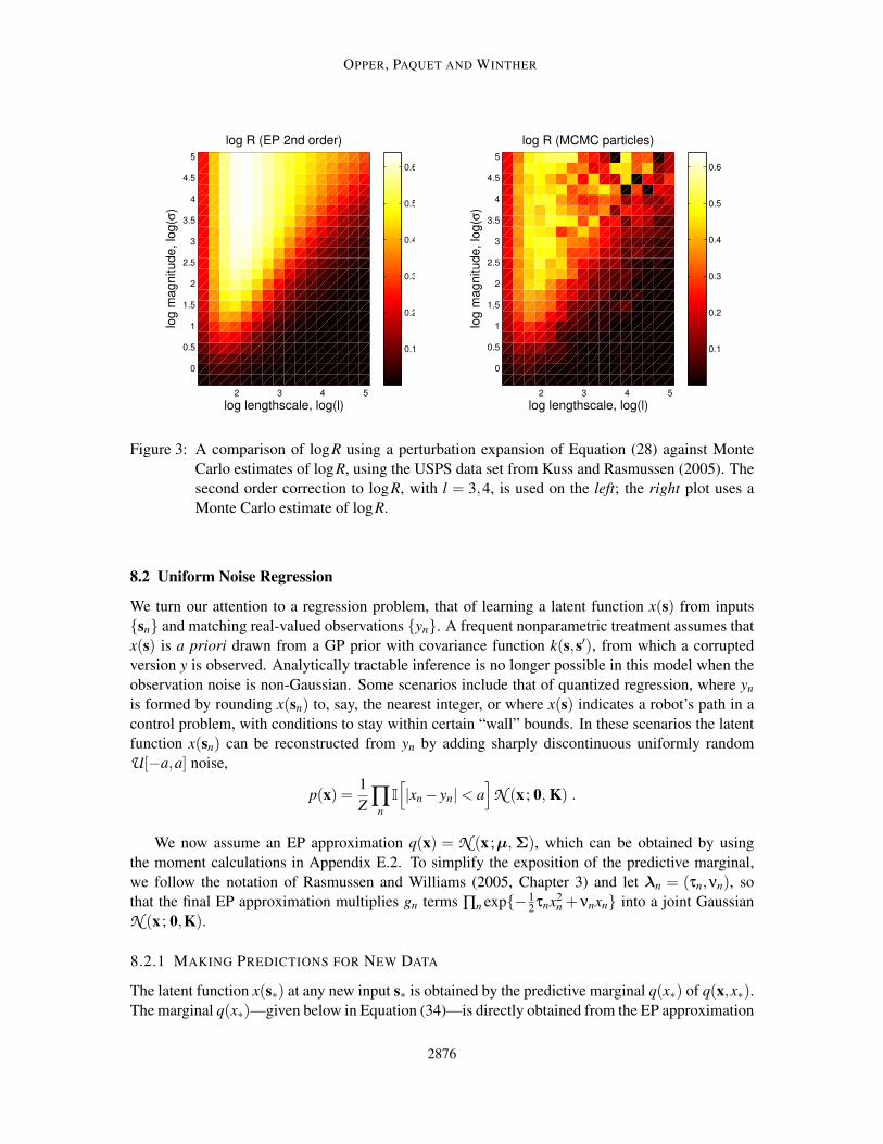
Figure 3 illustrates the correction to logR, with l = 3,4, on the binary subproblem of the USPS
3’s vs. 5’s digits data set, with N = 767. This is the same set-up of Kuss and Rasmussen (2005) and
Opper et al. (2009), using the kernel k(s,s′) = σ2 exp(− 12‖s− s′‖2/ℓ2), and we refer the reader to
both papers for additional and complimentary figures and results. We evaluated Equation (28) on a
similar grid of logℓ and logσ values. For the same grid values we obtained Monte Carlo estimates
of logZ, and hence logR. The correction, compared to the magnitude of the logZ grids by Kuss
and Rasmussen (2005), is remarkably small, and underlines their findings on the accuracy of EP for
GPC.
The correction from Equation (28), as computed here, is O(N2), and compares favorably to
O(N3) complexity of EP for GPC.
2875
OPPER, PAQUET AND WINTHER
2 3 4 5
0
0.5
1
1.5
2
2.5
3
3.5
4
4.5
5
log R (EP 2nd order)
log lengthscale, log(l)
log
ma
gn
itu
de
, lo
g(σ
)
0.1
0.2
0.3
0.4
0.5
0.6
2 3 4 5
0
0.5
1
1.5
2
2.5
3
3.5
4
4.5
5
log R (MCMC particles)
log lengthscale, log(l)
log
ma
gn
itu
de
, lo
g(σ
)
0.1
0.2
0.3
0.4
0.5
0.6
Figure 3: A comparison of logR using a perturbation expansion of Equation (28) against Monte
Carlo estimates of logR, using the USPS data set from Kuss and Rasmussen (2005). The
second order correction to logR, with l = 3,4, is used on the left; the right plot uses a
Monte Carlo estimate of logR.
8.2 Uniform Noise Regression
We turn our attention to a regression problem, that of learning a latent function x(s) from inputs
{sn} and matching real-valued observations {yn}. A frequent nonparametric treatment assumes that
x(s) is a priori drawn from a GP prior with covariance function k(s,s′), from which a corrupted
version y is observed. Analytically tractable inference is no longer possible in this model when the
observation noise is non-Gaussian. Some scenarios include that of quantized regression, where yn
is formed by rounding x(sn) to, say, the nearest integer, or where x(s) indicates a robot’s path in a
control problem, with conditions to stay within certain “wall” bounds. In these scenarios the latent
function x(sn) can be reconstructed from yn by adding sharply discontinuous uniformly random
U[−a,a] noise,
p(x) =1
Z∏
n
I
[
|xn − yn|< a]
N (x ; 0, K) .
We now assume an EP approximation q(x) = N (x ;µ,Σ), which can be obtained by using
the moment calculations in Appendix E.2. To simplify the exposition of the predictive marginal,
we follow the notation of Rasmussen and Williams (2005, Chapter 3) and let λn = (τn,νn), so
that the final EP approximation multiplies gn terms ∏n exp{− 12τnx2
n + νnxn} into a joint Gaussian
N (x ; 0,K).
8.2.1 MAKING PREDICTIONS FOR NEW DATA
The latent function x(s∗) at any new input s∗ is obtained by the predictive marginal q(x∗) of q(x,x∗).The marginal q(x∗)—given below in Equation (34)—is directly obtained from the EP approximation
2876
PERTURBATIVE CORRECTIONS FOR APPROXIMATE INFERENCE
q(x) = N (x ;µ,Σ). However, the correction to its mean, as was given in Equation (29), requires
covariances Σ∗n, which are derived here.
Let κ∗ = k(s∗,s∗), and k∗ be a vector containing the covariance function evaluations k(s∗,sn).Again following Rasmussen and Williams (2005)’s notation, let Σ be the diagonal matrix containing
1/τn along its diagonal. The EP covariance, on the inclusion of x∗, is
Σ∗ =
([K k∗kT∗ κ∗
]−1
+
[Σ
−1 0
0T 0
])−1
=
[Σ k∗−K(K+ Σ)−1k∗
kT∗ −kT
∗ (K+ Σ)−1K κ∗−kT∗ (K+ Σ)−1k∗
]
, (33)
with Σ = K−K(K+ Σ)−1K. There is no observation associated with s∗, hence τ∗ = 0 in the first
line above, and its inclusion has cl∗ = 0 for l ≥ 3. The second line follows by computing matrix
partitioned inverses twice on Σ∗. The joint EP approximation for any new input point s∗ is directly
obtained as
q(x,x∗) = N
([x
x∗
]
;
[µ
kT∗ K−1µ
]
,Σ∗
)
,
with the marginal q(x∗) being
q(x∗) = N (x∗ ; kT∗ K−1µ, κ∗−kT
∗ (K+ Σ)−1k∗) = N (x∗ ; µ∗, σ2∗) . (34)
According to Equation (29), one needs the covariances Σ∗ j to correct the marginal’s mean; they
appear in the last column of Σ∗ in Equation (33). The correction is
〈x∗〉p(x,x∗)−µ∗ = ∑l≥3
∑j 6=n
Σ∗ j
Σ j j
cl+1, jcln
l!
(Σ jn
Σ j jΣnn
)l
+ · · · .
The sum over pairs j 6= n include the added dimension ∗, and thus pairs ( j,∗) and (∗,n). The
cumulants for this problem, used both for EP and correcting it, are derived in Appendix E.2.
8.2.2 PREDICTIVE CORRECTIONS
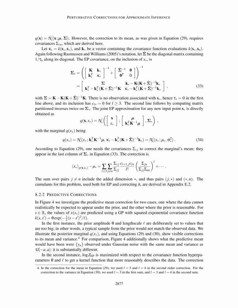
In Figure 4 we investigate the predictive mean correction for two cases, one where the data cannot
realistically be expected to appear under the prior, and the other where the prior is reasonable. For
s ∈ R, the values of x(s∗) are predicted using a GP with squared exponential covariance function
k(s,s′) = θexp(− 12(s− s′)2/ℓ).
In the first instance, the prior amplitude θ and lengthscale ℓ are deliberately set to values that
are too big; in other words, a typical sample from the prior would not match the observed data. We
illustrate the posterior marginal q(x∗), and using Equations (29) and (30), show visible corrections
to its mean and variance.4 For comparison, Figure 4 additionally shows what the predictive mean
would have been were {yn} observed under Gaussian noise with the same mean and variance as
U[−a,a]: it is substantially different.
In the second instance, logZEP is maximized with respect to the covariance function hyperpa-
rameters θ and ℓ to get a kernel function that more reasonably describes the data. The correction
4. In the correction for the mean in Equation (29), we used l = 3 and l = 4 in the second order correction. For the
correction to the variance in Equation (30), we used l = 3 in the first sum, and l = 3 and l = 4 in the second sum.
2877
OPPER, PAQUET AND WINTHER
−2.5 −2 −1.5 −1 −0.5 0 0.5 1 1.5 2 2.5−1
−0.8
−0.6
−0.4
−0.2
0
0.2
0.4
0.6
s
x(s
)
E[x*] from U[−a,a] noise (EP)
E[x*] from U[−a,a] noise (MCMC)
E[x*] + 2
nd order, U[−a,a] noise (EP+corr)
E[x*] +− two std dev, U[−a,a] noise (EP)
E[x*] +− two std dev, U[−a,a] noise (MCMC)
E[x*] +− two 2
nd order std dev, U[−a,a] (EP+corr)
E[x*] from N(0, a
2/3) noise (exact)
Figure 4: Predicting x(s∗) with a GP. The “boxed” bars indicate the permissible x(sn) values; they
are linked to observations yn through the uniform likelihood I[|xn − yn| < a]. Due to the
U[−a,a] noise model, q(x∗) is ambivalent to where in the “box” x(s∗) is placed. A second
order correction to the mean of q(x∗) is shown in a dotted line. The lightly shaded function
plots p(x∗), if the likelihood was also Gaussian with variance matching that of the “box”.
In the top figure both the prior amplitude θ and lengthscale ℓ are overestimated. In the
bottom figure, θ and ℓ were chosen by maximizing logZEP with respect to their values.
Notice the smaller EP approximation error.
to the mean of q(s∗) is much smaller, and furthermore, generally follows the “Gaussian noise”
posterior mean. When the observed data is not typical under the prior, the correction to 〈x∗〉 is
substantially bigger than when the prior is representative of the data.
2878
PERTURBATIVE CORRECTIONS FOR APPROXIMATE INFERENCE
−1 −0.5 0 0.5 1 1.5 2
−2
−1.5
−1
−0.5
0
0.5
1
1.5
2
s
x(s
)
−1 −0.5 0 0.5 1 1.5 2
−2
−1.5
−1
−0.5
0
0.5
1
1.5
2
s
x(s
)
E[x*] (EP)
E[x*] (MCMC)
E[x*] (EP+corr)
E[x*] +− 2σ (EP)
E[x*] +− 2σ (MCMC)
E[x*] +− 2σ (EP+corr)
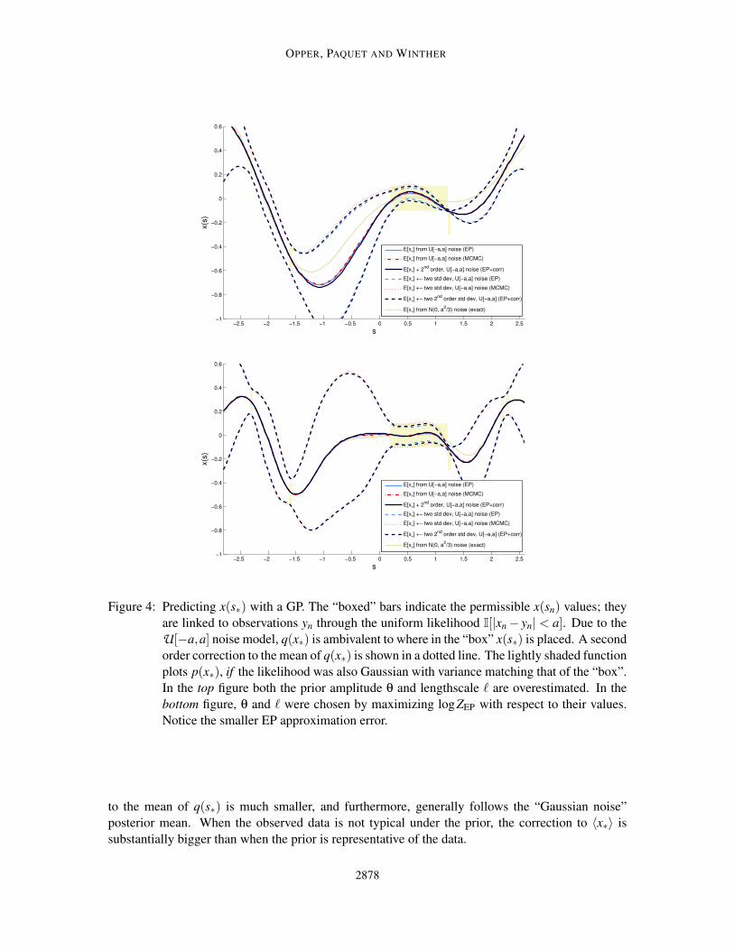
Figure 5: Predicting x(s∗) with a GP with k(s,s′) = exp{−|s− s′|/2ℓ} and ℓ = 1. In the left figure
logRMCMC = 0.41, while the second order correction estimates it as logR ≈ 0.64. On
the right, the correction to the variance is not as accurate as that on the left. The right
correction is logRMCMC = 0.28, and its discrepancy with logR ≈ 0.45 (EP+corr) is much
bigger.
8.2.3 UNDERESTIMATING THE TRUTH
Under closer inspection, the variance in Figure 4 is slightly underestimated in regions where there
are many close box constraints |xn − yn| < a. However, under sparser constraints relative to the
kernel width, EP accurately estimates the predictive mean and variance. In Figure 5 this is taken
further: for N = 100 uniformly spaced inputs s ∈ [0,1], it is clear that q(x) becomes too narrow. The
second order correction, on the other hand, provides a much closer estimate to the ground truth.
One might inquire about the behavior of the EP estimate as N → ∞ in Figure 5. In the next
section, this will be used as a basis for illustrating a special case where logZEP diverges.
8.3 Gaussian Process in a Box
In the following insightful example—a special case of uniform noise regression—logZEP diverges
from the ground truth with more data. Consider the ratio of functions x(s) over [0,1], drawn from
a GP prior with kernel k(s,s′), such that x(s) lies within the [−a,a] box. Figure 6 illustrates three
random draws from a GP prior, two of which are not contained in the [−a,a] interval. The ratio of
functions contained in the interval is equal to the normalizing constant of
p(x) =1
Z∏
n
I
[
|xn|< a]
N (x ; 0, K) . (35)
The fraction of samples from the GP prior that lie inside [−a,a] shouldn’t change as the GP is
sampled at increasing granularity of inputs s. As Figure 6 illustrates, the MCMC estimate of logZ
converges to a constant as N → ∞. The EP estimate logZEP, on the other hand, diverges to −∞.
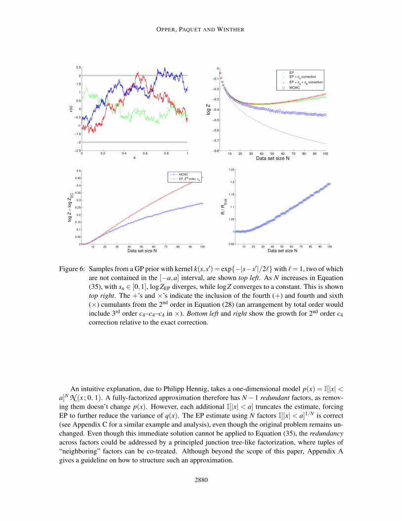
(The cumulants that are required for the correction in Equation (28), and recipes for deriving them,
are given in Appendix E.1.) Of course the correction also depends on the value a chosen. Figure 7
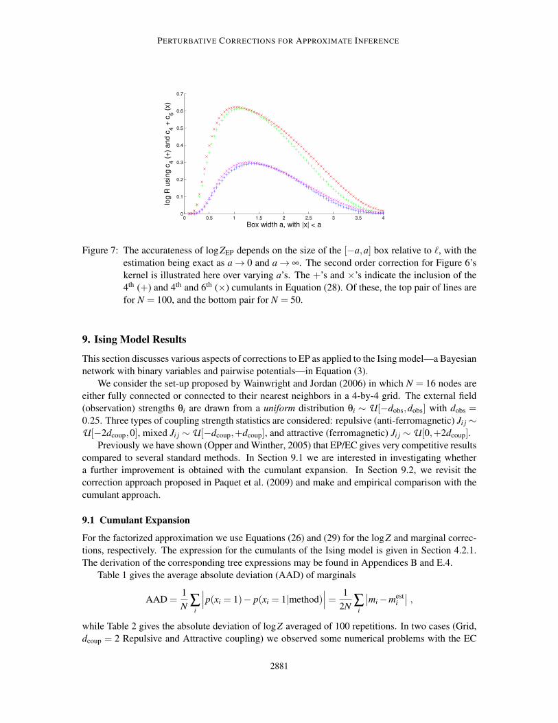
shows that for both a → 0 and a → ∞ the correction is zero for large N.
2879
OPPER, PAQUET AND WINTHER
0 0.2 0.4 0.6 0.8 1−2.5
−2
−1.5
−1
−0.5
0
0.5
1
1.5
2
2.5
s
x(s
)
10 20 30 40 50 60 70 80 90 100−0.8
−0.7
−0.6
−0.5
−0.4
−0.3
−0.2
−0.1
0
Data set size N
log
Z
EP
EP + c4 correction
EP + c4 + c
6 correction
MCMC
10 20 30 40 50 60 70 80 90 1000
0.05
0.1
0.15
0.2
0.25
0.3
0.35
0.4
0.45
0.5
Data set size N
log Z
− log Z
EC
MCMC
EP, 2nd
order, c4
10 20 30 40 50 60 70 80 90 1000.95
1
1.05
1.1
1.15
1.2
1.25
Data set size N
R /
Rtr
ue
Figure 6: Samples from a GP prior with kernel k(s,s′) = exp{−|s−s′|/2ℓ} with ℓ= 1, two of which
are not contained in the [−a,a] interval, are shown top left. As N increases in Equation
(35), with sn ∈ [0,1], logZEP diverges, while logZ converges to a constant. This is shown
top right. The +’s and ×’s indicate the inclusion of the fourth (+) and fourth and sixth
(×) cumulants from the 2nd order in Equation (28) (an arrangement by total order would
include 3rd order c4–c4–c4 in ×). Bottom left and right show the growth for 2nd order c4
correction relative to the exact correction.
An intuitive explanation, due to Philipp Hennig, takes a one-dimensional model p(x) = I[|x|<a]N N (x ; 0, 1). A fully-factorized approximation therefore has N −1 redundant factors, as remov-
ing them doesn’t change p(x). However, each additional I[|x| < a] truncates the estimate, forcing
EP to further reduce the variance of q(x). The EP estimate using N factors I[|x| < a]1/N is correct
(see Appendix C for a similar example and analysis), even though the original problem remains un-
changed. Even though this immediate solution cannot be applied to Equation (35), the redundancy
across factors could be addressed by a principled junction tree-like factorization, where tuples of
“neighboring” factors can be co-treated. Although beyond the scope of this paper, Appendix A
gives a guideline on how to structure such an approximation.
2880
PERTURBATIVE CORRECTIONS FOR APPROXIMATE INFERENCE
0 0.5 1 1.5 2 2.5 3 3.5 40
0.1
0.2
0.3
0.4
0.5
0.6
0.7
Box width a, with |x| < a
log R
usin
g c
4 (
+)
and c
4 +
c6 (
x)
Figure 7: The accurateness of logZEP depends on the size of the [−a,a] box relative to ℓ, with the
estimation being exact as a → 0 and a → ∞. The second order correction for Figure 6’s
kernel is illustrated here over varying a’s. The +’s and ×’s indicate the inclusion of the
4th (+) and 4th and 6th (×) cumulants in Equation (28). Of these, the top pair of lines are
for N = 100, and the bottom pair for N = 50.
9. Ising Model Results
This section discusses various aspects of corrections to EP as applied to the Ising model—a Bayesian
network with binary variables and pairwise potentials—in Equation (3).
We consider the set-up proposed by Wainwright and Jordan (2006) in which N = 16 nodes are
either fully connected or connected to their nearest neighbors in a 4-by-4 grid. The external field
(observation) strengths θi are drawn from a uniform distribution θi ∼ U[−dobs,dobs] with dobs =0.25. Three types of coupling strength statistics are considered: repulsive (anti-ferromagnetic) Ji j ∼U[−2dcoup,0], mixed Ji j ∼ U[−dcoup,+dcoup], and attractive (ferromagnetic) Ji j ∼ U[0,+2dcoup].
Previously we have shown (Opper and Winther, 2005) that EP/EC gives very competitive results
compared to several standard methods. In Section 9.1 we are interested in investigating whether
a further improvement is obtained with the cumulant expansion. In Section 9.2, we revisit the
correction approach proposed in Paquet et al. (2009) and make and empirical comparison with the
cumulant approach.
9.1 Cumulant Expansion
For the factorized approximation we use Equations (26) and (29) for the logZ and marginal correc-
tions, respectively. The expression for the cumulants of the Ising model is given in Section 4.2.1.
The derivation of the corresponding tree expressions may be found in Appendices B and E.4.
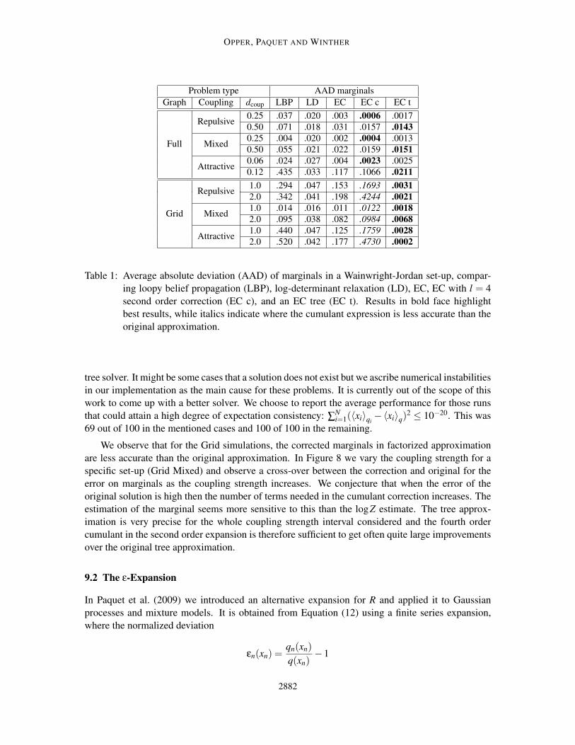
Table 1 gives the average absolute deviation (AAD) of marginals
AAD =1
N∑
i
∣∣∣p(xi = 1)− p(xi = 1|method)
∣∣∣=
1
2N∑
i
∣∣mi −mest
i
∣∣ ,
while Table 2 gives the absolute deviation of logZ averaged of 100 repetitions. In two cases (Grid,
dcoup = 2 Repulsive and Attractive coupling) we observed some numerical problems with the EC
2881
OPPER, PAQUET AND WINTHER
Problem type AAD marginals
Graph Coupling dcoup LBP LD EC EC c EC t
Full
Repulsive0.25 .037 .020 .003 .0006 .0017
0.50 .071 .018 .031 .0157 .0143
Mixed0.25 .004 .020 .002 .0004 .0013
0.50 .055 .021 .022 .0159 .0151
Attractive0.06 .024 .027 .004 .0023 .0025
0.12 .435 .033 .117 .1066 .0211
Grid
Repulsive1.0 .294 .047 .153 .1693 .0031
2.0 .342 .041 .198 .4244 .0021
Mixed1.0 .014 .016 .011 .0122 .0018
2.0 .095 .038 .082 .0984 .0068
Attractive1.0 .440 .047 .125 .1759 .0028
2.0 .520 .042 .177 .4730 .0002
Table 1: Average absolute deviation (AAD) of marginals in a Wainwright-Jordan set-up, compar-
ing loopy belief propagation (LBP), log-determinant relaxation (LD), EC, EC with l = 4
second order correction (EC c), and an EC tree (EC t). Results in bold face highlight
best results, while italics indicate where the cumulant expression is less accurate than the
original approximation.
tree solver. It might be some cases that a solution does not exist but we ascribe numerical instabilities
in our implementation as the main cause for these problems. It is currently out of the scope of this
work to come up with a better solver. We choose to report the average performance for those runs
that could attain a high degree of expectation consistency: ∑Ni=1(〈xi〉qi
−〈xi〉q)2 ≤ 10−20. This was
69 out of 100 in the mentioned cases and 100 of 100 in the remaining.
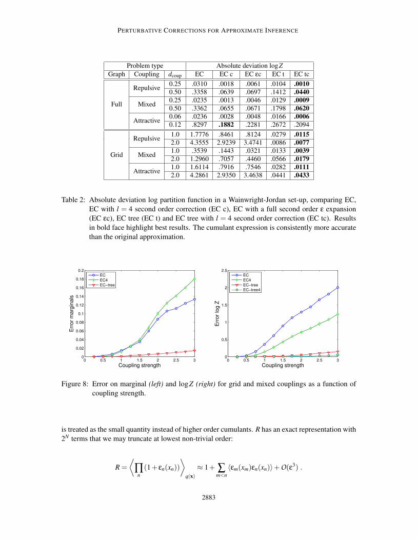
We observe that for the Grid simulations, the corrected marginals in factorized approximation
are less accurate than the original approximation. In Figure 8 we vary the coupling strength for a
specific set-up (Grid Mixed) and observe a cross-over between the correction and original for the
error on marginals as the coupling strength increases. We conjecture that when the error of the
original solution is high then the number of terms needed in the cumulant correction increases. The
estimation of the marginal seems more sensitive to this than the logZ estimate. The tree approx-
imation is very precise for the whole coupling strength interval considered and the fourth order
cumulant in the second order expansion is therefore sufficient to get often quite large improvements
over the original tree approximation.
9.2 The ε-Expansion
In Paquet et al. (2009) we introduced an alternative expansion for R and applied it to Gaussian
processes and mixture models. It is obtained from Equation (12) using a finite series expansion,
where the normalized deviation
εn(xn) =qn(xn)
q(xn)−1
2882
PERTURBATIVE CORRECTIONS FOR APPROXIMATE INFERENCE
Problem type Absolute deviation logZ
Graph Coupling dcoup EC EC c EC εc EC t EC tc
Full
Repulsive0.25 .0310 .0018 .0061 .0104 .0010
0.50 .3358 .0639 .0697 .1412 .0440
Mixed0.25 .0235 .0013 .0046 .0129 .0009
0.50 .3362 .0655 .0671 .1798 .0620
Attractive0.06 .0236 .0028 .0048 .0166 .0006
0.12 .8297 .1882 .2281 .2672 .2094
Grid
Repulsive1.0 1.7776 .8461 .8124 .0279 .0115
2.0 4.3555 2.9239 3.4741 .0086 .0077
Mixed1.0 .3539 .1443 .0321 .0133 .0039
2.0 1.2960 .7057 .4460 .0566 .0179
Attractive1.0 1.6114 .7916 .7546 .0282 .0111
2.0 4.2861 2.9350 3.4638 .0441 .0433
Table 2: Absolute deviation log partition function in a Wainwright-Jordan set-up, comparing EC,
EC with l = 4 second order correction (EC c), EC with a full second order ε expansion
(EC εc), EC tree (EC t) and EC tree with l = 4 second order correction (EC tc). Results
in bold face highlight best results. The cumulant expression is consistently more accurate
than the original approximation.
0 0.5 1 1.5 2 2.5 30
0.02
0.04
0.06
0.08
0.1
0.12
0.14
0.16
0.18
0.2
Coupling strength
Err
or
marg
inals
EC
EC4
EC−tree
0 0.5 1 1.5 2 2.5 30
0.5
1
1.5
2
2.5
Coupling strength
Err
or
log Z
EC
EC4
EC−tree
EC−tree4
Figure 8: Error on marginal (left) and logZ (right) for grid and mixed couplings as a function of
coupling strength.
is treated as the small quantity instead of higher order cumulants. R has an exact representation with
2N terms that we may truncate at lowest non-trivial order:
R =
⟨
∏n
(1+ εn(xn))
⟩
q(x)
≈ 1+ ∑m<n
〈εm(xm)εn(xn)〉+O(ε3) .
2883
OPPER, PAQUET AND WINTHER
The linear terms are all equal to one because⟨
qn(xn)q(xn)
⟩
q=
∫q(xn)
qn(xn)q(xn)
dxn = 1 and since qn(xn) is a
binary distribution the quadratic term becomes a weighted sum of ratios of Normal distributions:
⟨qm(xm)
q(xm)
⟩
q(x)
= ∑xn,xm=±1
1+ xmmm
2
1+ xnmn
2
q(xm,xn)
q(xm)q(xn).
The final expression for the lowest order approximation to R is then
R ≈ 1+ ∑m<n
∑xn,xm=±1
1+ xmmm
2
1+ xnmn
2
q(xm,xn)
q(xm)q(xn)− N(N −1)
2.
From Table 2 we observe an improvement over the original factorized approximation and results
similar to the cumulant correction to the factorized approximation for all settings. The ε-expansion
may also used to calculate marginals and applied to generalized factorizations. These topics will be
studied elsewhere.
10. Future Directions
Corrections to Gaussian EP approximations were examined in this paper. The Gaussian measure
allowed for a convenient set of mathematical tools to be employed, mostly because it admits or-
thogonality of a set of polynomials, the Hermite polynomials, which allowed a clean simplification
of many expressions. So far we have restricted ourselves to expansions to low orders in cumulants.
Our results indicate that these first corrections to EP can already provide useful information about
the quality of the EP solution. Small corrections typically show that EP is fairly accurate and the
corrections improve on that. On the other hand, large corrections indicate that the EP approximation
performs poorly. The low order corrections can yield a step in the right direction but in general their
result may not be trusted and alternatives to the Gaussian EP approximation should be considered.
It will be interesting to develop similar expansions to EP approximations with other exponential
families besides the Gaussian one.
Can we expect that higher order terms in the cumulant expansion will give more reliable approx-
imations? Before such a question could be attacked one first would need to decide in which order
the terms of the expansion should be evaluated in order to obtain the most dominant contributions.
For example, we might think of trying to first compute all terms in the second order expansion of
the exponential in Equation (26), and then move on to higher orders. An alternative is to sort the
expansion by the total sum of the orders of cumulants involved. This is in fact possible by intro-
ducing a suitable expansion parameter (which is later set equal to one) such that the formal Taylor
series with respect to this parameter yields the desired expansion. However, it is not clear yet if and
when such a power series expansion would actually converge. It may well be that our expansions
are only of an asymptotic type (Boyd, 1999) for which the summation of only a certain number of
terms might give an improvement whereas further terms would lead to worse results.
We expect that such questions could at least be answered for toy models such as the Gaussian
process in a box model of Section 8.3. Our results for the latter example (together with the related
uniform noise regression case) indicates that EP may not be understood as an off the shelf method
for approximately calculating arbitrary high dimensional sums or integrals. One may conjecture
that its quality strongly depends on the fact that such sums or integrals may or may not have an
interpretation in terms of a proper statistical inference model which contain data that are highly
2884
PERTURBATIVE CORRECTIONS FOR APPROXIMATE INFERENCE
probable with respect to the model. It would be interesting to see if one can develop a theory for the
average case performance of EP under such statistical assumptions of the data.
Appendix A. Factorizations: Gaussian Examples
As p(x) is a latent Gaussian model, the g-terms in Equation (5) are chosen in this paper to give a
Gaussian approximation
q(x) =1
Zq
exp{λT φ(x)}= N (x ; µ,Σ) .
The sufficient statistics φ(x) and natural parameters λ of the Gaussian are defined as
φ(x) = (x,− 12xxT ) and λ= (γ,Λ) ,
where λT φ(x) = γT x− 12
tr[ΛxxT ] = γT x− 12xT
Λx. There exists a bijection between the canonical
parameters µ and Σ and natural parameters, such that the mean and covariance can be determined
with Σ=Λ−1 and µ=Σγ.
In Equation (1) we can define g0(x) = exp{λT0 φ(x)}, where λ0 = (γ(0),Λ(0)), such that it is
essentially a rescaling of factor f0. In the Ising model in Equation (3), this means that Λ(0) =−J and
γ(0) = θ. In the Gaussian process classification model in Equation (2), this implies that Λ(0) = K−1
and γ(0) = 0.
A.1 Term-Wise Factorizations
It remains to define a suitable factorization for the term-product ∏n tn(xn). This factorization can
be fully factorized, factorized over disjoint sets of variables, factorized as a tree, or follow more
arbitrary factorizations (see the simple example in Appendix C). A few such factorizations are
given below in increasing orders of complexity. In each case we do not include the f0 factor for
clarity. Furthermore, even though the term factorization may be chosen to fully factorize, q(x) may
be fully connected through the inclusion of f0.
A.1.1 FULLY FACTORIZED
A common factorization of ∏n tn(xn) is to set fn(x) = tn(xn). The natural parameters of gn(x) =
exp{λTn φ(x)} are chosen to be λn = (γ
(n)n ,Λ
(n)nn ), corresponding to φn(xn) = (xn,− 1
2x2
n). For clarity
the other γ and Λ parameters in λn are not shown, as they are clamped at zero. This gives an
approximation q(x) that is defined by λ= λ0 +∑nλn.
A.1.2 FACTORIZATION INTO DISJOINT PAIRS
As a second step the N variables can be subdivided into disjoint pairs xπ = (xm,xn). The factoriza-
tion over terms couples pairs of variables through
∏n
tn(xn) = ∏π=(m,n)
[ tm(xm)tn(xn) ] = ∏π
fπ(x) .
In this case each factor will have a contribution gπ(x) = exp{λTπφ(x)} to the overall approximation,
and, as gπ is a function of two variables, it is parameterized by the “correlated Gaussian form”
λπ = (γ(π)m ,γ
(π)n ,Λ
(π)mm ,Λ
(π)nn ,Λ
(π)mn ). By symmetry Λ
(π)nm = Λ
(π)mn . The resulting q(x) is defined in
terms of these disjoint sets with λ= λ0 +∑πλπ.
2885
OPPER, PAQUET AND WINTHER
A.1.3 TREE-STRUCTURED FACTORIZATION
A tree structure factorization can be defined by extending the above “disjoint pairs” case to allow
for overlaps between terms. Let G define a spanning tree structure over all x, and let τ = (m,n)∈ Gdefine the edges in the tree. Let dn be the number of edges emanating from node xn in the graph.
Through a clever regrouping of terms into a “junction tree” form with
∏n
tn(xn) =∏τ=(m,n)[ tm(xm)tn(xn) ]
∏n tn(xn)dn−1=
∏τ fτ (x)
∏n fn(x)dn−1,
the term-approximation will be tree-structured. In this example the Da powers are 1 for edge factors
fτ and (1− dn) for node factors fn. Let gτ (x) and gn(x) be parameterized by λτ and λn, as was
done in the two examples above. Using
∏τ gτ (x)
∏n gn(x)dn−1=
∏τ exp{λTτφ(x)}
∏n exp{λTn φ(x)}dn−1
,
the resulting q(x) has parameter vector λ= λ0 +∑τ λτ −∑n(dn −1)λn.
It is useful to note that the form of the tree-structured approximation given here is that used by
Opper and Winther (2005); it approximates the “junction tree” form using a Power EP factorization
(Minka, 2004). The factorization and stationary condition is different from that of Tree EP (Minka
and Qi, 2004).
A.2 Stationary Point
The EP moment matching conditions from Equation (7) are uniquely met at the stationary point of
logZEP in Equation (8), and are shown here. Consider the logarithm of the normalizer,
logZEP = logZq +∑a
Da logZa . (36)
Using the sufficient statistics and natural parameters defined above, the two normalizers that consti-
tute Equation (36) are
Zq =∫
e∑a DaλTa φ(x) dx ,
Za =1
Zq
∫e∑b Dbλ
Tb φ(x)−λT
a φ(x) fa(x)dx .
Using these definitions, the derivatives of the terms in Equation (36) with respect to some EP factor
c’s parameters λc are
∂ logZq
∂λc
= Dc 〈φ(x)〉q ,
∂ logZa
∂λc
=
{Dc 〈φ(x)〉qa
−Dc 〈φ(x)〉q if c 6= a
(Dc −1)〈φ(x)〉qc−Dc 〈φ(x)〉q if c = a .
When ∂ logZEP/∂λc = 0 for any c, the following therefore holds:
0 = (Dc −1)(〈φ(x)〉qc−〈φ(x)〉q)+ ∑
a 6=c
Da(〈φ(x)〉qa−〈φ(x)〉q) .
2886
PERTURBATIVE CORRECTIONS FOR APPROXIMATE INFERENCE
Let D be a square matrix where the values in column a are Da; all the rows in D are equal and it is
singular. Furthermore, let ψa = 〈φ(x)〉qa−〈φ(x)〉q. By stacking all the ψa’s into a column vector
ψ, the above set of equalities lead to a system of equations
0 = ((D− I)⊗ Idim)ψ .
(The Kronecker product is only required as the sufficient statistics’ differences ψa have dimension-
ality “dim”, usually larger than one.) As D− I is nonsingular, it is solved by ψ = 0, and hence
〈φ(x)〉qa= 〈φ(x)〉q for all a.
The choice of parameterization of λa might give an overcomplete representation, and the exact
moment-matching conditions 〈φ(x)〉qa= 〈φ(x)〉q might have more than one unique solution. How-
ever, this does not invalidate that at the stationary point of Equation (36), all moment-matching
conditions must hold.
Appendix B. Tree-Structured Approximation
Let the factorization of the term-product ∏n tn(xn) take the form of a tree G with edges τ = (m,n)∈G , as is described in Appendix A.1.3. The number connections to a node or vertex n shall be denoted
by dn. From Equation (32) the second order expansion is
logR =1
2∑
τ 6=τ ′〈〈rτ 〉〈rτ ′〉〉+ 1
2∑
m6=n
(1−dm)(1−dn)〈〈rm〉〈rn〉〉
+∑τ ,n
(1−dn)〈〈rτ 〉〈rn〉〉+1
2∑n
(1−dn)(−dn)⟨
〈rn〉2⟩
+ · · · , (37)
where the inner expectations are over kτ |x and kn|x, while the outer expectations are over x.5 The
edge-edge, edge-node, and node-node expectations that are needed in Equation (37) are given in the
following three sections.
B.1 Edge-Edge Expectations
The edge-edge expectation provides a beautiful illustration of the combinatorics that may be in-
volved in Wick’s theorem. For τ 6= τ ′, the following expectation needs to be evaluated:
〈〈rτ (kτ )〉〈rτ ′(kτ ′)〉〉
=
⟨
∑l≥3
∑s≥3
il+s
{
∑|α|=l
cατ
α!〈kα
τ 〉kτ |x
}{
∑|α′|=s
cα′τ ′
α′!
⟨
kα′τ ′
⟩
kτ′ |x
}⟩
x
. (38)
The vectors α that are summed over to get |α| = l are α = (0, l),(1, l − 1), . . . ,(l,0); let α =(α1, l −α1) when |α|= l. From the independence of kτ |x and kτ ′ |x,
⟨
〈kατ 〉kτ |x 〈k
α′τ ′ 〉k
τ′ |x
⟩
x=⟨
〈kατ kα′
τ ′ 〉kτ ,kτ′ |x
⟩
x=⟨
kα1τ1
kl−α1τ2
kα′
1
τ′1k
s−α′1
τ′2
⟩
kτ ,kτ′, (39)
5. Some readers might wonder why there is no 12 associated with the sum over (τ ,n) in Equation (37). In the other
quadratic sums, for example over m 6= n, each (m,n) pair appears twice, as rmrn and as rnrm. Each edge-node pair
makes only one appearance in the sum; if the sum double-counted by including node-edge pairs, a division by two
would have been necessary.
2887
OPPER, PAQUET AND WINTHER
and therefore 〈〈rτ 〉〈rτ ′〉〉= 〈〈rτ rτ ′〉〉 whenever τ 6= τ ′.Wick’s theorem is again instrumental in computing 〈kα
τ kα′τ ′ 〉, as all possible pairings of the ran-
dom variables kτ = (kτ1,kτ2
) and kτ ′ = (kτ′1,kτ′2
) need to be included. As 〈k2τ1〉 = 0, 〈kτ1
kτ2〉 =
0, 〈k2τ′1〉 = 0, and 〈kτ′1
kτ′2〉 = 0, the only non-zero expectations in the Wick expansion of Equa-
tion (39) occur when all the variables in kτ and kτ ′ are paired. This immediately means that
〈kα1τ1
kl−α1τ2
kα′
1
τ′1k
s−α′1
τ′2〉 = 0 whenever l 6= s, as there will be some remaining variables in kτ (or kτ ′)
that can’t be paired and have to be self-paired with zero expectation.
Given l = s, evaluate the expectation in Equation (39). We introduce the “pairing count” vector
β with elements β j ∈N0 and constraint ∑4j=1 β j = l. Let β1 count the number of pairings of kτ1
with
kτ′1, and β2 count the number of pairings of kτ1
with kτ′2. As there are α1 kτ1
terms, the sum of its
outgoing pairings should equal α1 with
β1 +β2 = α1 .
A furthermore requirement is that
β1 +β3 = α′1 , β3 +β4 = α2 , β2 +β4 = α′
2 ,
where α2 = l −α1 and α′2 = l −α′
1, and β3 and β4 be as in the Wick expansion below. Define Bto be the set of all such β’s, and let C (β) count the number of permuted configurations for a given
pairing β. From Wick’s theorem the expected value is equal to the sum over all possible pairings β:
⟨
kα1τ1
kα2τ2
kα′
1
τ′1k
α′2
τ′2
⟩
kτ ,kτ′= ∑
β∈B
C (β)〈kτ1kτ′1
〉β1〈kτ1kτ′2
〉β2〈kτ2kτ′1
〉β3〈kτ2kτ′2
〉β4 .
A simple scheme to enumerate all β ∈ B is to let
β =[
β1, α1 −β1, α′1 −β1, (l +β1)− (α1 +α′
1)]
,
so that β ∈ B for each β1 ∈ {max(0,(α1 +α′1)− l), . . . ,min(α1,α
′1)}. The remaining components
of β are uniquely determined from β1.
B.1.1 COUNTING PAIRINGS
How many permuted pairings C (β) are there?
1. There are(
α1
β1
)ways of choosing β1 kτ1
’s, and thenα′
1!
(α′1−β1)!
ways of choosing kτ′1to pair with.
2. This leaves a remaining (α1 −β1) kτ1’s, that need to be paired with (l −α′
1) kτ′2’s. There are
(l−α′1)!
((l−α′1)−(α1−β1))!
such pairings.
3. There are also α′1 −β1 remaining kτ′1
’s, that need to be paired with kτ2variables. There are
(l−α1
α′1−β1
)ways of picking a kτ2
, and a further (α′1 −β1)! ways of arranging the remaining kτ′1
.
4. Finally, the (l −α′1)− (α1 −β1) remaining k′τ2
s need to be coupled with the remaining kτ′2’s,
and there are ((l −α′1)− (α1 −β1))! such arrangements.
2888
PERTURBATIVE CORRECTIONS FOR APPROXIMATE INFERENCE
Multiplying the possible pairings from the four steps above gives
C (β) =
(α1
β1
)α′
1!
(α′1 −β1)!
(l −α′1)!
((l +β1)− (α1 +α′1))!
· · ·
· · ·×(
l −α1
α′1 −β1
)
(α′1 −β1)! ((l +β1)− (α1 +α′
1))!
=
(α1
β1
)
α′1! (l −α′
1)!
(l −α1
α′1 −β1
)
,
which adds up to the total number of possible pairings ∑β∈B C (β) = l!. A further useful simplifi-
cation is C (β)/α!α′! = 1/β! when |α|= |α′|= l, and is used below.
B.1.2 EDGE-EDGE EXPECTATION
The absence of any self-interacting loops from Wick’s theorem lets the ∑s≥3 drop away in Equation
(38), as all terms are zero except for when l = s. Substituting 〈kατ kα′
τ ′ 〉 and C (β) into Equation (38)
gives the final result,
〈〈rτ (kτ )〉〈rτ ′(kτ ′)〉〉
= ∑l≥3
(−1)l ∑|α|=l
∑|α′|=l
cατ cα′τ ′
{
∑β∈B
1
β!〈kτ1
kτ′1〉β1〈kτ1
kτ′2〉β2〈kτ2
kτ′1〉β3〈kτ2
kτ′2〉β4
}
.
B.2 Edge-Node Expectations
The derivation for the edge-node expectations is similar to that of the edge-edge case,
〈〈rτ (kτ )〉〈rn(kn)〉〉=⟨
∑l≥3
∑s≥3
il+s ∑|α|=l
cατ csn
α! s!〈kα
τ 〉kτ |x 〈ksn〉kn|x
⟩
x
= ∑l≥3
(−1)l ∑|α|=l
cατ cln
α!〈kτ1
kn〉α1 〈kτ2kn〉l−α1 ,
where the expectations in the last line are again over {kτ ,kn}. When 〈kατ ks
n〉 is evaluated with
Wick’s theorem, there are α1 copies of kτ1, l−α1 copies of kτ2
, and s copies of kn. The zero relation
of kτ and kn ensures that the only non-zero terms in the Wick sum are those where all the kτ’s are
paired with kn’s; in other words, when l = s. There are l! possible pairings, which cancels l! in the
denominator.
The above edge-node expectation is for any edge and node in the tree, but notice that it simplifies
greatly when the edge τ is a connection to node n. Say τ1 is the edge variable corresponding to xn.
In this case the covariance with respect to the opposite pair is zero, with 〈kτ2,kn〉= 0 (see Figure 2)
and only one of the α’s will have a non-zero contribution to the sum, namely when α= (l,0).
B.3 Node-Node Expectations
The node-node expectation is given in Equation (27), and is also used for 〈〈rn〉2〉.6
6. Due to the square in 〈〈rn〉2kn|x〉x
, the inner average 〈rn〉kn|x should first be computed to give an expansion over Hermite
polynomials in xn − µn. An example of such a result is given Appendix C. The orthogonality of these polynomials
over q(x−µ) allows 〈〈rn〉2kn|x〉x
to also reduce to Equation (27).
2889
OPPER, PAQUET AND WINTHER
Appendix C. A Tractable, One-Dimensional Example
The following example illustrates a tractable one-dimensional model with two factors. It is shown
analytically that the correction to logZEP must be zero, and that the result is reflected in the higher-
order terms in Equation (32), which are also zero.
Consider the factorization of a probit term with a Gaussian prior into
p(x) =1
ZΦ(x)N (x;0,1) =
1
Zfa(x)
1/2 fb(x)1/2N (x;0,1) ,
where Φ(x) is the cumulative Gaussian density function, and fa(x) = fb(x) = Φ(x). Z can be
computed exactly, but for the sake of example p(x) will be approximated with
q(x) =1
Zq
ga(x)1/2gb(x)
1/2N (x;0,1) = N (x;µ,σ2) .
Choose ga(x) = exp{φ(x)Tλa}, and gb(x) = exp{φ(x)Tλb}. The q approximation has parameter
vector λ= λ0 +12λa +
12λb. The EP fixed point is defined by λa = λb and Za = Zb. (For example,
subtracting λa at the fixed point will leave λ\a = λ0 + 0, which is equal to a scaled version of the
prior f0(x). The factor fa(x) = Φ(x) is hence incorporated into the prior, giving Za. By a symmetric
argument, Za = Zb.) Although it is trivial to show that ZEP = ZqZ1/2a Z
1/2
b will be equal to the true
partition function Z, we shall prove it by showing that the correction term is logR = 0.
C.1 Analytic Correction
In this section a transformation of variables from x to y ∼ N (y;0,1), with y = (x− µ)/σ, will be
used to make the derivation slightly simpler, and therefore
ka|y ∼ N
(
ka ; − iy
σ, σ−2
)
, kb|y ∼ N
(
kb ; − iy
σ, σ−2
)
.
Below we analytically show that the correction logR is zero, and hence that
R =
⟨⟨
era(ka)⟩1/2
ka|y
⟨
erb(kb)⟩1/2
kb|y
⟩
y
=⟨√
Fa(y)√
Fb(y)⟩
y= 1 , (40)
where Fa(y) is a shorthand for 〈era(ka)〉ka|y and
ra(ka) = ∑l≥3
ilcal
l!kl
a , rb(kb) = ∑l≥3
ilcbl
l!kl
b .
Because fa = fb, the cumulants will be the same for all l, hence cal = cbl . Furthermore, ka|y and
kb|y are both distributed according to the same density. Now define, using era = 1+ ra +12r2
a + · · · ,
Fa(y) =
⟨
1+∑l≥3
ilcal
l!kl
a +1
2∑
l,s≥3
il+s calcas
l!s!kl+s
a + · · ·⟩
ka|y
=
⟨
1+∑l≥3
cal
l!
(1
σ
)l
(y+ iu)l +1
2∑
l,s≥3
calcas
l!s!
(1
σ
)l+s
(y+ iu)l+s + · · ·⟩
u
= 1+∑l≥3
cal
l!
(1
σ
)l
Hl(y)+1
2∑
l,s≥3
calcas
l!s!
(1
σ
)l+s
Hl+s(y)+ · · · (41)
2890
PERTURBATIVE CORRECTIONS FOR APPROXIMATE INFERENCE
In the second line above a transformation of variables was made in the integral, with u = σka + iy,
such that ka = (u− iy)/σ. The Jacobian 1/σ ensures proper normalization so that the average is
over u ∼ N (u;0,1). In the last line Hl(y) is the Hermite polynomial of degree l,
which can be obtained for any real y and integer l = 0,1,2, . . . from the average Hl(y) =⟨(y+ iu)l
⟩
u
over u ∼ N (u;0,1).7
The remarkable property 〈Hl(y)〉y = 0 for all l, ensures that 〈Fa(y)〉y = 1 in Equation (41). Fur-
thermore, Fa(y) = Fb(y) follows from the equivalence in cumulants cal = cbl; the roots in Equation
(40) disappear to give 〈Fa(y)〉y, proving that R = 1 in Equation (40).
C.2 Second Order Correction
The second order expansion in Equation (32) in Section 7 evaluates to zero, as the matching cumu-
lants cal = cbl and equal distributions of ka|x and kb|x ensure that 〈ra(ka)〉ka|x = 〈rb(kb)〉kb|x:
logR =1
4
⟨
〈ra(ka)〉ka|x 〈rb(kb)〉kb|x
⟩
x− 1
8
(⟨
〈ra(ka)〉2ka|x
⟩
x+⟨
〈rb(kb)〉2kb|x
⟩
x
)
+ · · ·
=1
4
⟨
〈ra(ka)〉2ka|x
⟩
x− 1
8
(
2⟨
〈ra(ka)〉2ka|x
⟩
x
)
+ · · ·
= 0+ · · · .
Appendix D. Corrections to Marginals Distributions
Corrections to the marginal distributions follow from a similar derivation to that of the normalizing
constant. As a simplification, let the Gaussian approximation be centred with y = x−µ, so that
q(y)=N (y ; 0,Σ), and assume that q(x) is arises from the fully factorized approximation in Section
5. In this appendix corrections will be computed for the mean 〈xi −µi〉p(x) = 〈yi〉p(y), and variance⟨(xi −µi)(x j −µ j)−Σi j
⟩
p(x)=⟨yiy j
⟩
p(y)−Σi j.
A further simplification that will be employed in the following section is a change of variables
ηn = kn + iΣ−1nn yn, so that ηn ∼ N (ηn ; 0, Σ−1
nn ). Let
zn = ηn − iΣ−1nn yn ,
which is zero-mean complex Gaussian random variable with a relation⟨z2
n
⟩= 0 and 〈zmzn〉 =
−Σmn/(ΣmmΣnn) when m 6= n. Following Equation (24), the correction reads
R =
⟨
∏n
⟨
rn(kn)⟩
kn|yn
⟩
y
=
⟨
∏n
⟨
rn
(
ηn − iΣ−1nn yn
)⟩
ηn
⟩
y
=
⟨
exp
[
∑n
rn(zn)
]⟩
z
.
7. When F (y) in Equation (41) is rearranged as a power series in σl , we obtain an Edgeworth expansion to arbitrary
order l. The deviation from the Gaussian q(y) is thereby factorized out of tilted distribution with qa(y) = q(y)F (y).The interested reader is pointed to Blinnikov and Moessner (1998).
2891
OPPER, PAQUET AND WINTHER
D.1 The Marginal Mean
The lowest order correction to the EP marginal’s mean follows from the result in Equation (13):
〈yi〉p(y) =1
R
⟨
yi e∑n rn(zn)⟩
z
=1
R∑
j
Σi j
⟨∂
∂y j
e∑n rn(zn)
⟩
=1
R∑
j
Σi j
⟨
∂
∂y j
(
1+∑n
rn(zn)+1
2∑m,n
rm(zm)rn(zn)+ · · ·)⟩
=1
R∑
j
Σi j
⟨∂r j(z j)
∂y j
+∑n
rn(zn)∂r j(z j)
∂y j
+ · · ·⟩
.
In the above expansion the first order term is∂r j(z j)
∂y j=
∂r j(z j)∂z j
∂z j
∂y j= −iΣ−1
j j
∂r j(z j)∂z j
, and disappears as⟨
∂r j(z j)∂z j
⟩
= 0. The j = n second order term also disappears as⟨
r j(z j)∂r j(z j)
∂z j
⟩
= 0. These equiv-
alences can be seen by taking r j(z j) (and also its derivative) as a expansion over powers of z j; as
〈z2j〉= 0, Wick’s theorem states that every expectation of powers of z j should be zero. Hence
〈yi〉p(y) =− i
R∑j 6=n
Σi j
Σ j j
⟨
rn(zn)∂r j(z j)
∂z j
⟩
z
+ · · · . (42)
The derivative of the characteristic function, as required in Equation (42), is
∂r j(z j)
∂z j
=∂
∂z j
[
∑l≥3
ilcl j
l!zl
j
]
= i ∑l≥3
il−1 cl j
(l −1)!zl−1
j = i ∑l≥2
ilcl+1, j
l!zl
j .
The expectations for j 6= n in Equation (42) evaluate to
⟨
rn(zn)∂r j(z j)
∂z j
⟩
z
= i ∑s,l≥3
is+l cl+1, j,csn
l!s!
⟨
zljz
sn
⟩
+ i ∑s≥3,l=2
is+l cl+1, j
2!s!
⟨
zljz
sn
⟩
= i ∑l≥3
i2l cl+1, jcln
(l!)2
⟨
zljz
ln
⟩
, (43)
with the second term disappearing as s > l = 2 ensures that some zn is always self-paired in Wick’s
theorem. Finally, by substituting Equation (43) into (42), the correction to the mean is
〈yi〉p(y) = ∑l≥3
∑j 6=n
Σi j
Σ j j
cl+1, jcln
l!
(Σ jn
Σ j jΣnn
)l
±·· · .
2892
PERTURBATIVE CORRECTIONS FOR APPROXIMATE INFERENCE
D.2 The Marginal Covariance
The correction to the second moments follow the same recipe as that of the marginal mean in
Appendix D.1. We proceed by first treating yi with
⟨yiy j
⟩
p(y)=
1
R
⟨
yi
{
y j e∑n rn(zn)}⟩
z
=1
R∑k
Σik
⟨∂
∂yk
{
y j e∑n rn(zn)}⟩
=1
R∑k
Σik
⟨
δ jk e∑n rn(zn)+ y j
∂
∂yk
e∑n rn(zn)
⟩
= Σi j +1
R∑k
Σik
⟨
y j
∂
∂yk
e∑n rn(zn)
⟩
.
Reapplying the recipe gives the correction to the covariance:
⟨yiy j
⟩
p(y)−Σi j =
1
R∑kl
ΣilΣ jk
⟨∂2
∂yk∂yl
e∑n rn(zn)
⟩
z
=−i∑kl
Σil
Σll
Σ jk
⟨∂
∂yk
∂rl(zl)
∂zl
e∑n rn(zn)
⟩
+ · · ·
=−∑kl
Σil
Σll
Σ jk
Σkk
⟨[
δkl
∂2rl(zl)
∂z2l
+∂rk(zk)
∂zk
∂rl(zl)
∂zl
]
e∑n rn(zn)
⟩
= ∑s≥3
∑k 6=l
ΣilΣ jl
Σ2ll
cskcs+2,l
s!
(Σkl
ΣkkΣll
)s
+ ∑s≥3
∑k 6=l
Σil
Σll
Σ jk
Σkk
cskcsl
s!
(Σkl
ΣkkΣll
)s−1
+ · · · .
Appendix E. Higher Order Cumulants
Much of this paper hinges on cumulants beyond the second order. These are frequently more cum-
bersome to obtain than the initial moments that are required by EP. This appendix provides details
of the cumulants used in this paper.
The cumulants of a distribution qn(x) can be obtained from its moments through
c3 =⟨x3⟩−3⟨x2⟩〈x〉+2〈x〉3 ,
c4 =⟨x4⟩−4⟨x3⟩〈x〉−3
⟨x2⟩2
+12⟨x2⟩〈x〉2 −6〈x〉4 ,
c5 =⟨x5⟩−5⟨x4⟩〈x〉−10
⟨x3⟩⟨
x2⟩+20
⟨x3⟩〈x〉2 +30
⟨x2⟩2 〈x〉−60
⟨x2⟩〈x〉3 +24〈x〉5
;
they are derived for doubly-truncated Gaussian distributions in Appendices E.1 and E.2. One might
also directly take derivatives of the cumulant generating function, and the cumulants of a Probit-
times-Gaussian distribution, common to GP classification models, are derived this way in Appendix
E.3.
The tree-structured approximation in Sections 7 and 9.1, and Appendices A.1.3 and B, require
cumulants over two variables. They are presented in Appendix E.4 for the Ising model.
2893
OPPER, PAQUET AND WINTHER
E.1 Doubly Truncated Centered Gaussian
Consider the centered distribution qn(xn) ∝ I[|xn| < a]N (xn ; 0, λ−1n ). The odd moments of this
tilted distributions are, by symmetry, 〈xn〉=⟨x3
n
⟩=⟨x5
n
⟩= 0. Let
Zn = 2
√
λ
2π
∫ a
0e−
12
λx2
dx = 2Φ(z)−1 , z =√
λa ,
with the Probit function being Φ(x) =∫ x−∞ N (z;0,1)dz. Subscripts n are dropped where they are
clearly implied by their context. To get the even moments, consider
A1 = ∂λ logZn = ∂λ log
(√λ
∫ a
−adxe−
12
λx2
)
=1
2λ− 1
2
⟨x2⟩,
A2 = ∂2λ logZn =− 1
2λ2+
1
4
(⟨x4⟩−⟨x2⟩2)
.
Using the partition function, we get
A1 = ∂λ log(2Φ(z)−1) =a√λ
(N (z)
2Φ(z)−1
)
,
A2 =a2
2λ
(zN (z)
2Φ(z)−1
)
− a
2λ3/2
(N (z)
2Φ(z)−1
)
− a2
λ
(N (z)
2Φ(z)−1
)2
,
and thus
⟨x2⟩=
1
λ−2A1 ,
⟨x4⟩=
2
λ2+⟨x2⟩2
+4A2 .
We can further determine A3 = ∂3λ logZn using the partition function, giving
A3 =3a
4λ5/2
(N (z)
2Φ(z)−1
)
+3a2
4λ2
(zN (z)
2Φ(z)−1
)
+3a2
2λ2
(N (z)
2Φ(z)−1
)2
+2a3
λ3/2
(N (z)
2Φ(z)−1
)3
+3a3
2λ3/2
(N (z)
2Φ(z)−1
)(zN (z)
2Φ(z)−1
)
+a3
4λ3/2
((z2 −1)N (z)
2Φ(z)−1
)
.
Therefore⟨x6⟩=
8
λ3+⟨x2⟩⟨
x4⟩−2⟨x2⟩3
+2⟨x4⟩⟨
x2⟩−8A3 .
E.2 Doubly Truncated Non-Centered Gaussian
The same calculation from Appendix E.1 can be repeated to get the moments of the non-centered
truncated Gaussian qn(xn) ∝ I[|xn|< a]N (xn ; µ, λ−1n ). The subscripts n are dropped where evident.
The partition function is
Z(λ,µ) =
√
λ
2π
∫ a
−ae−
12
λ(x−µ)2
dx = Φ(zmax)−Φ(zmin) ,
2894
PERTURBATIVE CORRECTIONS FOR APPROXIMATE INFERENCE
−3 −2.5 −2 −1.5 −1 −0.5 0 0.5 1 1.5 20
0.05
0.1
0.15
0.2
0.25
0.3
0.35
0.4
0.45
0.5
log(σ2)
Gaussian N(x ; 0.5 , σ2) in box |x| < a, with a = 1.0
E[x]
E[x2]
E[x3]
E[x4]
E[x5]
Figure 9: The moments of qn(x) ∝ I[|x| < a]N (x ; µ, σ2), as a function of σ2. As the Gaussian
variance σ2 → ∞, the moments converge to that of a uniform U[−a,a] distribution.
where
zmax =√
λ(µ+a) , zmin =√
λ(µ−a) .
By again taking increasing derivatives of Z(λ,µ) with respect to µ and λ, the moments solved for
are
〈x〉= µ+1√λ
N (zmax)−N (zmin)
Φ(zmax)−Φ(zmin),
⟨x2⟩= 2〈x〉µ+
1
λ−µ2 − 1
λ
zmaxN (zmax)− zminN (zmin)
Φ(zmax)−Φ(zmin),
⟨x3⟩= 3
⟨x2⟩
µ+ 〈x〉[
3
λ−3µ2
]
− 3
λµ+µ3 ,
− 1
λ3/2
(1− z 2max)N (zmax)− (1− z 2
min)N (zmin)
Φ(zmax)−Φ(zmin),
⟨x4⟩= 4
⟨x3⟩
µ+⟨x2⟩[
2
λ−6µ2
]
+ 〈x〉[
4µ3 − 4
λµ
]
+2
λµ2 −µ4 +
1
λ2
− 1
λ2
zmax(1+ z2max)N (zmax)− zmin(1+ z2
min)N (zmin)
Φ(zmax)−Φ(zmin).
Finally,
⟨x5⟩= 5
⟨x4⟩
µ+⟨x3⟩[
6
λ−10µ2
]
+⟨x2⟩[
10µ3 − 18
λµ
]
+ 〈x〉[
18
λµ2 −5µ4 − 3
λ2
]
+3
λ2µ
− 6
λµ3 +µ5 − 1
λ5/2
(1+2z2max − z4
max)N (zmax)− (1+2z2min − z4
min)N (zmin)
Φ(zmax)−Φ(zmin).
As Figure 9 illustrates, these moments will converge to that of a uniform distribution as the Gaus-
sian’s variance grows large.
2895
OPPER, PAQUET AND WINTHER
m
log(σ
)
Cumulant c3 with m=0 and v=0 (step function)
−6 −4 −2 0 2 4 6−1
−0.8
−0.6
−0.4
−0.2
0
0.2
0.1
0.2
0.3
0.4
0.5
0.6
0.7
m
log(σ
)
Cumulant c4 with m=0 and v=0 (step function)
−6 −4 −2 0 2 4 6−1
−0.8
−0.6
−0.4
−0.2
0
0.2
−0.6
−0.5
−0.4
−0.3
−0.2
−0.1
0
0.1
0.2
0.3
Figure 10: The third and fourth cumulants of the density qn(x) ∝ Φ((x−m)/v)N (x;µ,σ2) in Ap-
pendix E.3. The step function Θ(x), with m = v = 0, is taken as an example here. The
third cumulant is always positive, while the fourth cumulant is positive only when σ> µ.
E.3 Probit Link Cumulants
EP approximations to Probit regression models, and Gaussian process classification models in gen-
eral (see Section 8.1), depend on the moments of qn(x) ∝ Φ((x−m)/v)N (x;µ,σ2). We introduce
v ≥ 0 so that the likelihood can become a step function at v = 0, for example. We shall obtain the
cumulants by taking derivatives of the characteristic function. The characteristic function of qn(x),as described by Equation (15), is
χn(k) =⟨eikx⟩
qn(x)= exp
{
ikµ− 1
2k2σ2
}Φ(zk)
Φ(z),
with
z =µ−m√v2 +σ2
, zk =µ+ ikσ2 −m√
v2 +σ2.
The cumulants cln are determined from the derivatives of logχn(k) at zero; a lengthy calculation
shows that they are
c3n = α3β[2β2 +3zβ+ z2 −1
],
c4n =−α4β[6β3 +12zβ2 +7z2β+ z3 −4β−3z
],
where α = σ2/√
v2 +σ2 and β = N (z;0,1)/Φ(z).
E.4 Two-Variable Ising Model Cumulants
We need some third and fourth order two-variable cumulants and thus generalize the results of
Section 4.2 to the bivariate case. To do this we can exploit the cumulant generating property of
logχa(ka). Let c(l,l′) denote the joint l, l′ order cumulant of variable one and two, respectively. We
can generate this cumulant from derivatives of logχa(ka):
c(l,l′) =
(∂
∂ik1
)l(∂
∂ik2
)l′
logχa(ka)
∣∣∣∣∣k=0
.
2896
PERTURBATIVE CORRECTIONS FOR APPROXIMATE INFERENCE
We can also express this as a recursion in terms of cumulants:
c(l+n,l′+n′) =
(∂
∂ik1
)n(∂
∂ik2
)n′
c(l,l′)(k)
∣∣∣∣∣k=0
.
By explicit calculation for a bivariate binary distribution we get the first two orders’ cumulants: