Ecological Applications, 22(7), 2012, pp. 1936–1948� 2012 by the Ecological Society of America

Pest control experiments show benefits of complexityat landscape and local scales

REBECCA CHAPLIN-KRAMER1

AND CLAIRE KREMEN

Department of Environmental Science, Policy and Management, University of California, 130 Mulford Hall Number 3114,Berkeley, California 94720 USA

Abstract. Farms benefit from pest control services provided by nature, but managementof these services requires an understanding of how habitat complexity within and around thefarm impacts the relationship between agricultural pests and their enemies. Using cageexperiments, this study measures the effect of habitat complexity across scales on pestsuppression of the cabbage aphid Brevicoryne brassicae in broccoli. Our results reveal thatproportional reduction of pest density increases with complexity both at the landscape scale(measured by natural habitat cover in the 1 km around the farm) and at the local scale (plantdiversity). While high local complexity can compensate for low complexity at landscape scalesand vice versa, a delay in natural enemy arrival to locally complex sites in simple landscapesmay compromise the enemies’ ability to provide adequate control. Local complexity insimplified landscapes may only provide adequate top-down pest control in coolermicroclimates with relatively low aphid colonization rates. Even so, strong natural enemyfunction can be overwhelmed by high rates of pest reproduction or colonization from nearbysource habitat.

Key words: agroecosystems; biological control; Brevicoryne brassicae; cabbage aphid; ecosystemservices; natural habitat; pest management; Salinas Valley, California, USA.

INTRODUCTION

Natural enemies, the predators and parasitoids of

agricultural pests, provide a sustainable and efficient

alternative to pesticides in some circumstances (e.g., rice,

Settle et al. [1996]; cotton and citrus, Ruttan [1999]), but

fail strikingly to control pests under other circumstances

(Stiling 1993, Collier and Van Steenwyk 2004). Using

natural enemies instead of pesticides to control crop pests

could provide significant societal benefits by reducing

economic, environmental, and public health costs (Pi-

mentel et al. 1992, Eskenazi et al. 2007). To utilize natural

pest control services reliably, however, it is critical to

understand the conditions under which top-down control

can and cannot maintain pest populations below desired

levels. This study investigates landscape- and local-scale

environmental factors that constrain or enhance the

potential contribution of natural enemies in the manage-

ment of crop pests.

Both local- and landscape-scale factors are thought to

contribute to the control of pests by natural enemies.

While conservation biological control aims to maximize

pest control services by creating or enhancing habitat at

the local scale for native or ‘‘naturalized’’ natural

enemies (Fiedler et al. 2008), scientists now recognize

the importance of the larger landscape scale in

maintaining natural enemy communities (Tscharntke

et al. 2005). Structurally complex landscapes, defined as

landscapes with high proportions of natural or unman-

aged habitat, are associated with increased abundance

and diversity of natural enemies on farms, across many

different geographic locations and crop types (Bianchi et

al. 2006, Chaplin-Kramer et al. 2011b). The resources

provided for natural enemies in complex landscapes may

complement or substitute for local diversity in agro-

ecosystems (Tscharntke et al. 2005). The reverse may

not hold true, however. It has been suggested that local-

scale habitat improvements may not support a viable

natural enemy community on their own, but only serve

to concentrate enemies already supported by natural

habitat in the landscape surrounding the farm (Gurr et

al. 1998). Both scales are likely important to the

maintenance of healthy enemy communities, however,

and the interplay between them is not well understood.

Some studies have investigated the effects of complexity

at local and landscape scales simultaneously, but it has

proven difficult to resolve the relative contribution of

each factor (Elliott et al. 1998, Thies and Tscharntke

1999, Letourneau and Goldstein 2001, Ostman et al.

2001, Clough et al. 2005, Bianchi et al. 2008, Werling

and Gratton 2008). Local and landscape complexity are

also often correlated; small diverse farms tend to be

found in small wooded valleys and large monocultures

are more likely to be in vast agricultural areas.

Manuscript received 12 October 2011; revised 22 March2012; accepted 16 April 2012. Corresponding Editor: M. P.Ayres.

1 Present address: Natural Capital Project, StanfordUniversity, 371 Serra Mall, Stanford, California 94305USA. E-mail: bchaplin@stanford.edu

1936

An additional difficulty in understanding the rela-

tionship between pest control services and complexity at

any scale is that both direct and indirect effects can be

operating and may counteract one another. Habitat

complexity at either scale may benefit crop pests directly

if it provides alternate host plants or predator refuges

(Landis et al. 2000, Chaplin-Kramer et al. 2011a), or it

may constrain pests directly if it limits dispersal into or

across agricultural fields (den Belder et al. 2002).

Habitat complexity may also indirectly constrain pests

through enhancement of natural enemy communities

that provide top-down control (Tscharntke et al. 2005).

One step in understanding how habitat complexity

contributes to overall pest management is to determine

how it influences natural enemy populations, which in

turn affect pest population dynamics.

The vast majority of studies investigating the effects of

complexity on pest control services have stopped short

of actually measuring the service, instead using proxies

such as natural enemy abundance or predation rate

(Letourneau and Bothwell 2008, Chaplin-Kramer et al.

2011b). The first objective of this study is to determine

the degree to which natural enemies can reduce pest

populations, by measuring pest population growth in

the presence and absence of their enemies. The second

objective is to determine whether increased natural

enemy density or diversity associated with increased

habitat complexity confers enhanced pest control

services, by employing enemy exclusion experiments

across a complexity gradient. While previous studies

have utilized cage experiments to demonstrate enhanced

pest control services along landscape gradients

(Gardiner et al. 2009), no studies have compared the

effects of complexity across scales. Therefore, the

ultimate objective of this study is to measure differences

in pest control services provided by resident natural

enemies across a gradient of habitat complexity at two

scales. We test the hypotheses that (1) cross-scale habitat

complexity (i.e., complexity at both landscape and local

scales, compared to complexity at only one scale)

provides superior pest control services to farms, and

(2) one scale of complexity can substitute for another.

For the purposes of this paper, we draw a distinction

between pest control services and pest control. Pest

control is defined according to a predesignated threshold

known as the economic injury level, which has little to

do with the ecology or predator–prey dynamics of a

system. We define pest control services as the ecosystem

service that results in a reduction of pest populations

from the level they would achieve in the absence of that

service. For that reason, we focus more on comparative

measures of pest reduction rather than absolute

measures such as pest densities. We acknowledge that

pest control services as defined here may not always

result in economic pest control, but suggest that better

understanding the delivery of these services could be an

important step toward achieving more sustainable and

reliable pest management (Kremen 2005).

MATERIALS AND METHODS

Study system

The cabbage aphid Brevicoryne brassicae (Linnaeus) is

a major pest of broccoli. Aphids are able to build up

populations quickly following colonization because they

can reproduce asexually, giving birth to several live

young (nymphs) each day once they reach maturity.

There are alate (winged) and apterous (wingless) morphs

of adult aphids, with intraspecific competition triggering

the production of alate individuals, who then seek out

uncolonized plants and may spend several days produc-

ing nymphs before moving onto the next plant (Dixon

1977). The most abundant natural enemies of the

cabbage aphid in the study region are the larvae of

various syrphid flies (Diptera: Syrphidae). Other ene-

mies include the parasitic wasp Diaeretiella rapae,

coccinellid beetles (Coleoptera: Coccinellidae), the lace-

wings Chrysoperla and Hemerobius species, the aphid

midge Aphidoletes aphidimyza, spiders, and a variety of

other coleopteran and hemipteran predators (van

Emden 1963). Most of these enemies are extremely

mobile and forage in many different habitats for floral

resources and/or alternate prey, making floral resources

on farms or in the surrounding habitat an important

determinant of their distribution in crop fields.

Study sites

The study was conducted in 2008 and 2009 on 10

organic broccoli farms on California’s Central Coast, in

Santa Cruz, Monterey, and San Benito Counties (Fig.

1). The same sites were repeated across years and

seasons to avoid confounding spatial and temporal

variation (using the same fields within each farm

whenever possible, or the nearest field planted in

broccoli if crops were rotated in subsequent years).

The only pesticide used on broccoli at these sites was M-

PEDE (Dow AgroSciences, Indianapolis, Indiana,

USA), a nonpersistent insecticidal soap, which has been

shown to have temporary to no effects on natural

enemies (UC IPM 2008). At all sites, the crop around

the study area was not sprayed during the course of the

experiment. Study sites were characterized by the

amount of surrounding natural or seminatural habitat,

which included riparian habitat, chaparral scrub,

deciduous and coniferous woodland, and grasslands

that were often degraded and/or invaded by nonnative

weeds. Transects along farm field edges at each site

recorded the presence or absence of nearby weedy

patches of the mustard Brassica nigra, which may

provide a predator refuge for Brevicoryne brassicae

(Chaplin-Kramer et al. 2011a).

Sites were selected at either end of a landscape

complexity gradient, with the surrounding landscapes

composed of predominantly natural habitat (69% 6 8%natural habitat, 10% 6 7% agriculture, mean 6 SE) or

predominantly agricultural habitat (4% 6 2% natural

habitat, 69% 6 13% agriculture) within 1 km of the farm

October 2012 1937PEST CONTROL BENEFITS FROM COMPLEXITY

(established by weekly insect sampling over three years

to be the most predictive scale for B. brassicae in this

system; R. Chaplin-Kramer, P. de Valpine, N. J. Mills,

and C. Kremen, unpublished manuscript). This gradient

was fairly consistent across scales, with sites containing

either .50% natural habitat or ,10% natural habitat at

all scales from 0.5 to 3 km. Sites with high proportions

of natural or non-crop habitat in the surrounding

landscape would typically be defined as ‘‘complex’’

(measured at scales ranging from 0.5 to 6 km;

Tscharntke et al. 2005). Complexity can refer to both

the landscape and local scales, however, so we use

different terminology for clarity. Sites surrounded

predominantly by natural habitat are called ‘‘natural

matrix’’ landscapes and those surrounded predominant-

ly by agriculture are called ‘‘agricultural matrix’’

landscapes, referring to the dominant land use in these

landscapes. Four sites in each landscape category were

selected for study in 2008 (for a total sample size of N¼8), and one additional site in each category was included

in 2009 (N ¼ 10). All sites were at least 2 km apart,

maintaining independence at a landscape scale defined at

1 km (R. Chaplin-Kramer, P. de Valpine, N. J. Mills,

and C. Kremen, unpublished manuscript).

The study sites also differed in local habitat complex-

ity. ‘‘Locally complex’’ farms were characterized by

smaller fields (1.2–4 ha) planted with multiple (5–12)

crops, and the incorporation of non-crop floral re-

sources for beneficial insects in the form of hedgerows or

weed strips along the field edge. ‘‘Locally simple’’ farms

were large (6–12 ha) broccoli monocultures lacking any

non-crop habitat within the farm itself. Two farms of

each type of local category were selected for each

landscape category in the 2008 study. In 2009, three

locally complex farms were selected for each landscape

category, but no additional locally simple farms could be

added, due to limitations in farmer willingness to

participate.

The landscape surrounding the farms was character-

ized using Geographic Information Systems (ArcGIS,

version 9.3.1; Environmental Systems Research Insti-

tute, Redlands, California, USA). Aerial photographs at

1-m resolution were obtained through the National

Agricultural Imagery Project (2005 true-color version;

available online)2 for the area around each farm site. The

photographs were segmented using an object-based

FIG. 1. Map of study sites in Salinas Valley, California, USA, and surrounding areas. White areas correspond to agriculturalland, dark areas to urban/industrial/residential, and grays to different types of natural/seminatural habitat. Squares representlocally simple sites, and circles represent locally complex sites; open symbols represent agricultural matrix, while solid symbolsrepresent natural matrix.

2 http://www.apfo.usda.gov

REBECCA CHAPLIN-KRAMER AND CLAIRE KREMEN1938 Ecological ApplicationsVol. 22, No. 7

image analysis program with a scale parameter of 500, a

shape parameter of 0.1, and a smoothness parameter of

0.5 (eCognition, version 5.0; Definiens, Alexandria,

Virginia, USA). The resulting maps were classified by

hand to differentiate between agricultural, and natural

or seminatural habitat. Proportional areas were then

computed for each land-use class at a radius of 1 km

around the farm site using Hawth’s tools (version 3.27;

available online)3.

Experimental design

Broccoli plants were transplanted into pots from one-

month-old starts (acquired from Growers Transplant-

ing, Salinas, California, USA) in the greenhouse one

month prior to the start of each experiment; plants were

grown in identical conditions for early and late seasons

to maintain consistency across time periods. The potted

plants were then set out in cages (one plant per cage) at

each farm site for 12 days. Cages were either closed, with

all sides covered by mesh, or open, with two of the sides

left open (Appendix A). Data-loggers recorded temper-

ature and relative humidity at 10-min intervals in each

of the treatments at each site to assess microclimate

differences between open and closed cages (Hygrochron

I-buttons; Embedded Data Systems, Lawrenceburg,

Kentucky, USA). Temperature and relative humidity

were similar in both types of cages (19.58 6 0.78C vs.

18.68 6 0.78C, and 80.6% 6 1.7% vs. 83.9% 6 1.7%relative humidity; means 6 SE for closed vs. open cages,

respectively).

The potted broccoli plants used in this cage experi-

ment had identical initial aphid densities, to provide a

comparison of aphid growth in different locations with

and without natural enemies, independent of the natural

rate of aphid establishment. The one-month-old plants

were inoculated with 50 aphids each, to match the

normal range of 0–100 aphids per plant for plants of

that age in the field (Chaplin-Kramer 2010). Infested

leaves from greenhouse B. brassicae colonies were placed

on experimental plants, and the remaining aphids were

given several days to transfer from cut leaf to living

plant. The aphid populations on the experimental plants

reflected the age structure of the colony population,

which was consistently skewed toward the younger

instars (since reproductive adults produce several

nymphs per day); however, first and second instar

aphids were removed because wing buds could not be

detected in these early stages. Alate morphs and

individuals with wing buds were removed to ensure that

aphids would not leave the open cages during the course

of the experiment; we judged this procedure successful

since few (,5%) of the aphids found in the closed cages

at the end of the experiment were alate. Once the

transfer was complete, aphids on the experimental plants

were counted and aphids in excess of 50 were removed.

Aphids were recounted following transport of plants to

the field.

The experiments were carried out in August 2008 and

twice in 2009: in June, the early season before B.

brassicae populations peak in late July or August, and

again in August, the late season when aphid densities are

generally high across all regions (Chaplin-Kramer 2010).

Cages were arranged in groups (three per site in 2008,

two per site in 2009) at the edges of broccoli fields to

standardize for differences in field size (cf. Kremen et al.

2004). Each group had one closed cage, two open cages,

and one sentinel cage (identical in design to the open

cage, but not inoculated with aphids). This resulted in a

total of 12 cages (six open, three closed, three sentinel)

for each of the eight sites in 2008 (12 3 8 ¼ 96 cages

total), and eight cages (four open, two closed, two

sentinel) for each of the 10 sites over two time periods in

2009 (8 3 10 3 2 ¼ 160 cages total). More open cages

were included than closed or sentinel because open cages

showed the greatest variance in aphid population

growth in pilot studies.

The closed cages measured the population growth of

aphids in absence of predation over 12 days at each site.

The open cages measured the population growth of

aphids when exposed to predation and/or parasitism by

natural enemies. The sentinel cages measured net

colonization rate, the number of aphids arriving during

the course of the experiment (less the number of those

lost to predation or parasitism). As aphids only colonize

a plant as alate (winged) adults that can come and go

over the course of an experiment, the signal of

colonization is the immobile nymphs produced by these

transient adults. The reproductive rate of these coloniz-

ing aphids was assumed to match (or at least correlate

with) the reproductive rate found in the closed cages at

that site, and therefore was used to remove the

contribution of reproduction from that of colonization.

Few alate adults were found on the plants at the end of

the experiment (typically ,5 adults per plant); these

individuals when found were not included in the total to

avoid double-counting. There may also have been some

third-generation reproduction occurring on the sentinel

plants (if aphids born from colonizing adults reached

maturation during the study period), though the extent

of this would be minimal, as cabbage aphid generation

length is around 10 days for the field conditions in this

system (Hughes 1963). The colonization measured by

the uninfested sentinel plants is likely higher than would

be found on the pre-infested plants in the open cages, as

cabbage aphids have been found to prefer settling on

unoccupied plants in avoidance of induced plant

defenses (Prado and Tjallingii 2007). However, it is a

useful measure of initial colonization that newly planted

crops face in the field, and provides good indication of

how aphid colonization differs across sites.

Plants were harvested at the end of the 12 days.

Additionally, 150–250 g of leaf matter was collected at

each site along 20-m transects adjacent to the cages and3 http://www.spatialecology.com

October 2012 1939PEST CONTROL BENEFITS FROM COMPLEXITY

moving toward the interior of the field at the beginning

and end of the experiment. This provided a comparisonof insect densities (per gram of wet mass plant material)

in the cages vs. in the field. Experimental plants and leafmatter samples were individually bagged and brought

back to the laboratory for exhaustive counting of allinsect inhabitants. Natural enemies found in the open

cages included syrphid fly larvae, coccinellid beetles, andvarious spiders, a representative though less diversearray of enemies found in the broader fields at the sites

(Chaplin-Kramer 2010). However, because the opencages were designed specifically so that enemies could

easily enter and leave over the course of the experiment,we did not analyze predator densities or diversity within

the cages.

Pest control services

For the purposes of this experiment, pest control

services were defined as the ability of resident naturalenemies to constrain aphid population growth. This was

measured by the proportional reduction in aphid densityin the open cages as compared to the closed cages, which

were free of control from predators and parasitoids. Theproportional reduction in aphid density (PRD) for each

site j was calculated as

PRDj ¼ DOj=DCj ð1Þ

where DOj is site j’s final average density of aphids on the

plants in the open cages and DCj is site j’s final averagedensity of aphids in the closed cages. This measure of

PRD allows a clearer comparison between sites thanabsolute density (measured as aphid pressure, P, see

next paragraph) because it controls for inevitabledifferences in aphid settlement and population growthrate among sites, such as those that might be caused by

the presence of source populations or temperaturedifferences, which strongly affects aphid growth (Dixon

1977). PRD may underestimate total mortality becauseit does not account for aphid colonization in the open

cages, but as previously noted, the colonization mea-sured by sentinel cages is likely overestimated and

cannot be used as a proxy. Therefore, the pest reductionmeasured here can be considered a conservative

estimate.

Aphid pressure

The experimental design also allowed for additional

comparisons between sites, including factors such as pestreproduction and colonization. Net average reproduc-

tive rate (R) over 12 days for each site j was measured asthe change in aphid densities within the closed cages, or

Rj ¼ DCj=50 ð2Þ

where DCj is site j’s final average aphid density within theclosed cages and 50 is the initial aphid density within all

closed cages. Colonization (C ) at each site j wasmeasured as the average aphid density on the sentinel

plants (DSj) at the end of the experiment, normalized by

the average reproductive rate found at that site to avoid

double-counting reproduction:

Cj ¼ DSj=Rj: ð3Þ

As previously described, this formula captures the

arrival of alate adults that inhabited the plant long

enough to produce nymphs but departed before the end

of the experiment. Combining the total number of

aphids produced from reproduction with the total

number of aphids arriving from colonization provides

an idea of the overall aphid pressure (P) at each site ( j ):

Pj ¼ ðDCj � 50Þ þ Cj: ð4Þ

Insect densities in the surrounding field

Point-estimates of insect densities in the surrounding

field were achieved by counting aphids and natural

enemies found in the leaf matter collected from crops

adjacent to the cages, as a basis for comparison with the

information gained from the experiment. The only

natural enemy occurring at high enough densities for

reliable comparisons using this point-estimate method

was the syrphid fly larva. For better characterization of

the overall enemy community found at the field sites,

additional data were used from an insect survey

conducted between 2006 and 2008 at each of the sites

(Chaplin-Kramer 2010; R. Chaplin-Kramer, P. de

Valpine, N. J. Mills, and C. Kremen, unpublished

manuscript). In this broader insect survey, plants were

collected on a weekly basis at each site over three

summer growing seasons (ranging in mass from 50 g at

the beginning of the season to 1–2 kg at the end), and

insects were counted in a manner similar to that used for

the cage experiment. Average abundances (per gram of

plant material) of syrphid larvae, coccinellid beetles,

lacewings, aphid midges, and spiders were taken from

this more intensively sampled, three-year data set for

each site.

Analysis

All analyses were performed using generalized linear

mixed-effects models (GLMM) in the statistical pro-

gram R (package nlme, version 2.9.1; available online).4

Mixed-effects models were used to account for correla-

tion between repeated measurements at the same farm

sites (Gueorguieva and Krystal 2004). Site was therefore

included as a random effect for all mixed-effects models

for analyses on temperature, PRD, reproductive rate,

colonization, aphid pressure, and enemy abundance.

AICc scores (corrected for small sample size) were used

to select the best models, determining which factors

should be included in each analysis.

To determine whether there were systematic environ-

mental differences between the local and landscape

categories, maximum, minimum, and average daily

4 http://www.r-project.org

REBECCA CHAPLIN-KRAMER AND CLAIRE KREMEN1940 Ecological ApplicationsVol. 22, No. 7

temperatures recorded by the data-loggers at each site

were analyzed with landscape matrix, local complexity,

season, and year as fixed effects. Temperature data were

further tested as predictor variables for subsequent

analyses on reproductive rate, colonization, and aphid

pressure.

In order to meet the assumptions of linearity for the

GLMM, PRD was negative natural log (ln) transformed

for all analyses. Differences in �ln(PRD) were assessed

with colonization (C ), local complexity (simple or

complex), landscape matrix (natural or agricultural),

season (early or late), and year (2008 or 2009) as fixed

effects. Local by landscape matrix interactions were

included, as were interactions between each of these

factors, season and year.

Net reproductive rate (ln[R]) and colonization (ln[C])

were also each ln-transformed and analyzed with several

possible fixed effects and interactions, including land-

scape matrix, local complexity, season, year, and

temperature. The presence of weedy mustard (as a

potential refuge for aphids) was an additional factor

used in the analysis of colonization only.

Aphid pressure (P) was converted to a measure of P/

100 g of leaf material for comparison to field aphid

densities, and both measures were ln-transformed in a

simple linear model to test for a correlation between these

two variables. The natural logs of aphid pressure and

field aphid densities were also each analyzed in mixed-

effects models including the same potential variables as

the analysis for net reproductive rate and colonization

(see previous paragraph).

Point-estimate syrphid abundance in the surrounding

field and annual average natural enemy abundances for

the three years of survey data were each ln-transformed

and analyzed in mixed-effects models against landscape

matrix, local complexity, and interactions between these

two factors. The ln point-estimate syrphid abundance, ln

three-year average syrphid abundance, and ln three-year

average non-syrphid natural enemy abundance were also

included in mixed models (along with year and season)

against �ln(PRD) at each site in order to investigate

whether sites characterized by higher enemy densities

(both during the experiment and over a longer period

preceding it) received greater pest control services.

The replicate sites in each treatment of landscape or

local complexity may not be independent, as the

predominant agricultural area in this system is the

Salinas Valley, and the agricultural matrix sites are

therefore closer to each other than to the natural

matrix sites (Fig. 1). However, such spatial autocorre-

lation can be measured directly, with an analysis that

teases apart the variation in response variables ex-

plained by space alone from the variation explained by

other variables (in this case, habitat complexity at

landscape or local scales). Moran’s index quantifies the

degree of spatial autocorrelation in the data, using the

residuals from the model for each analysis in which

landscape or local factors were found to be significant

(following Lichstein et al. 2002, Kremen et al. 2004).

We therefore computed Moran’s index for any

variables that responded significantly to landscape

complexity.

RESULTS

Environmental differences

Average temperatures were higher in August 2008

than in August 2009 (19.58 6 0.78 vs. 17.28 6 0.38C), but

the differences in temperature between early and late

season in 2009 were minor (Appendix B). Landscape

and local complexity did not affect temperature.

Pest control services

There were significant local, landscape, and seasonal

effects on the proportional reduction of aphid densities,

PRD, as well as a significant interaction between

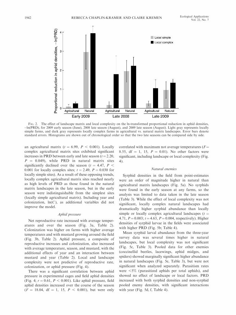
landscape and season (Table 1, Fig. 2). Specifically, in

the late season (August), the effect of local complexity in

the natural matrix landscape was not significant, but

locally complex sites had six times the PRD of locally

simple sites in the agricultural matrix landscape (t ¼2.48, P ¼ 0.031). Similarly, there was no significant

advantage of having a natural matrix at locally complex

sites, but natural matrix landscapes showed a more than

sixfold pest control advantage over agricultural matrix

landscapes at locally simple sites (t¼ 2.57, P¼ 0.026). In

contrast, local factors were not significant in the early

season (June). Landscape matrix type alone impacted

early-season PRD, with sites in a natural matrix

exhibiting orders of magnitude higher PRD of sites in

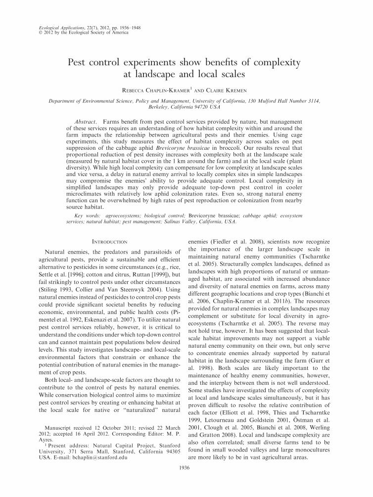
TABLE 1. Generalized linear mixed-effects model (GLMM) for fixed effects of landscape matrix, local complexity, and season onproportional reduction in aphid densities,�ln(PRD), with site as a random effect.

Variable Coefficient SE F P

Intercept (agricultural-simple-early) �0.20 0.34 �0.57 0.57Landscape (natural) 3.36 0.43 42.16 ,0.001Local (complex) 0.65 0.26 6.26 0.041Season (late) 0.69 0.38 5.71 0.030Landscape 3 season �2.61 0.54 23.32 ,0.001

Notes: For this and all subsequent tables, coefficients and standard errors (SE) are presented for each variable that contributedto the best model (based on AICc), and the reference levels of categorical variables are presented parenthetically. P values are alsopresented for all variables and interactions for the best model [�ln(PRD) ; landscape 3 timeþ local].

October 2012 1941PEST CONTROL BENEFITS FROM COMPLEXITY

an agricultural matrix (t ¼ 6.99, P , 0.001). Locally

complex agricultural matrix sites exhibited significant

increases in PRD between early and late season (t¼2.20,

P ¼ 0.049), while PRD in natural matrix sites

significantly declined over the season (t ¼ 4.47, P ,

0.001 for locally complex sites; t ¼ 2.49, P ¼ 0.030 for

locally simple sites). As a result of these opposing trends,

locally complex agricultural matrix sites reached nearly

as high levels of PRD as those found in the natural

matrix landscapes in the late season, but in the early

season were indistinguishable from the simplest sites

(locally simple agricultural matrix). Including year and

colonization, ln(C ), as additional variables did not

improve the model.

Aphid pressure

Net reproductive rate increased with average temper-

atures and over the season (Fig. 3a, Table 2).

Colonization was higher on farms with higher average

temperatures and with mustard growing around the field

(Fig. 3b, Table 2). Aphid pressure, a composite of

reproductive increases and colonization, also increased

with average temperature, season, and mustard, with the

additional effects of year and an interaction between

mustard and year (Table 2). Local and landscape

complexity were not predictive of reproductive rate,

colonization, or aphid pressure (Fig. 4).

There was a significant correlation between aphid

pressure in experimental cages and field aphid densities

(Fig. 4; r ¼ 0.61, P , 0.001). Like aphid pressure, field

aphid densities increased over the course of the season

(F ¼ 18.04, df ¼ 1, 15, P , 0.001), but were only

correlated with maximum not average temperatures (F¼8.55, df ¼ 1, 15, P ¼ 0.01). No other factors were

significant, including landscape or local complexity (Fig.

4).

Natural enemies

Syrphid densities in the field from point-estimates

were an order of magnitude higher in natural than

agricultural matrix landscapes (Fig. 5a). No syrphids

were found in the early season at any farms, so the

analysis was limited to data taken in the late season

(Table 3). While the effect of local complexity was not

significant, locally complex natural landscapes had

dramatically higher syrphid abundance than locally

simple or locally complex agricultural landscapes (t ¼4.71, P¼ 0.003; t¼ 4.63, P¼ 0.004, respectively). Higher

densities of syrphid larvae in the fields were associated

with higher PRD (Fig. 5b; Table 4).

Mean syrphid larval abundance from the three-year

survey data was several times higher in natural

landscapes, but local complexity was not significant

(Fig. 5c, Table 3). Pooled data for other enemies

(coccinellid beetles, lacewings, aphid midges, and

spiders) showed marginally significant higher abundance

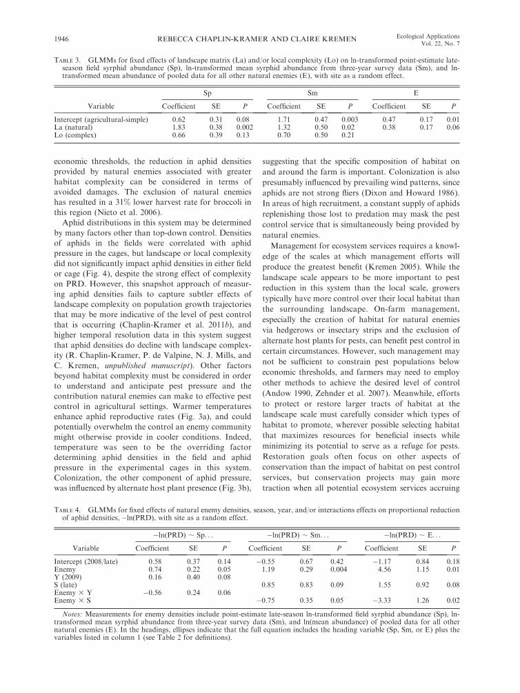
in natural landscapes (Fig. 5e, Table 3), but were not

significant when analyzed separately. Parasitism rates

were ,5% (parasitized aphids per total aphids), and

showed no effect of landscape or local factors. PRD

increased with both syrphid densities and non-syrphid

pooled enemy densities, with significant interactions

with year (Fig. 5d, f, Table 4).

FIG. 2. The effect of landscape matrix and local complexity on the ln-transformed proportional reduction in aphid densities,�ln(PRD), for 2009 early season (June), 2008 late season (August), and 2009 late season (August). Light gray represents locallysimple farms, and dark gray represents locally complex farms in agricultural vs. natural matrix landscapes. Error bars denotestandard errors. Histograms are shown out of chronological order so that the two late seasons can be compared side by side.

REBECCA CHAPLIN-KRAMER AND CLAIRE KREMEN1942 Ecological ApplicationsVol. 22, No. 7

Spatial autocorrelation

We found no significant spatial autocorrelationbetween sites for PRD or any of the measures of natural

enemy densities (Appendix C). That is, though allagricultural matrix sites were spatially clustered, the

clustering itself was not predictive of variation in thedata. The sites that were closest together were not the

most similar in terms of PRD or natural enemydensities. Average temperatures were also not autocor-

related. Minimum temperatures in early season 2009 didshow spatial autocorrelation (P , 0.001), but this effect

disappeared by the late season (Appendix C).

DISCUSSION

This study suggests that habitat complexity enhances

pest control services provided by natural enemies onfarms, and that complexity at the local scale (crop

diversity, floral resources) can substitute for that at thelandscape scale (natural habitat) or vice versa, late in theseason when pest populations are peaking. In the late

season, sites with high local complexity and low levels ofnatural habitat in the landscape matrix had proportional

reduction in aphid densities (PRD) equivalent to siteswith low local complexity and high levels of natural

habitat in the landscape matrix (Fig. 2). The PRD foundat these mixed-complexity sites was only slightly lower

than at the most complex sites (locally complex innatural matrix), but was substantially higher than the

simplest sites (locally simple in agricultural matrix). Thistrend was robust across years, though more pronounced

in 2008 than in 2009. The mixed-complexity sitesexhibited a proportional pest reduction an average of

six times greater than the simplest sites and notsignificantly different from the most complex sites. This

refutes our initial hypothesis that complexity at bothlandscape and local scales would enhance pest controlservices relative to complexity at only one scale, but

supports findings that local complexity provides greatervalue for natural enemy pest control in simpler

(agricultural) landscapes than in complex ones(Tscharntke et al. 2005, Haenke et al. 2009, O’Rourke

et al. 2011).The apparent substitutability of complexity across

scales in the late season was not evident in the earlyseason. The lower levels of PRD found in the early

season at the locally complex sites in agricultural matrixas compared to natural matrix indicate that the pest

control services provided by natural enemies may belagged at these sites. While PRD in the locally complex

agricultural landscapes subsequently ‘‘caught up’’ to thenatural landscapes by the late season, the low levels of

pest reduction at these sites in the early season suggeststhat the ability of enemies to constrain aphid popula-

tions may be seriously compromised. Aphid densities inthis system can increase by several orders of magnitudefrom early-season to the late-season aphid peak

(Chaplin-Kramer 2010). If enemies can better constrainaphids at the low densities that occur early in the season,

the subsequent aphid peak may be less pronounced.

However, a delay in enemy response to aphid arrival

may create a window of opportunity for rapid and

unchecked aphid population growth. Indeed, previous

work has demonstrated that predation during the early

stages of aphid establishment determines total popula-

tion and ultimately crop yields more so than predation

later in the season (Ostman et al. 2001).

In our study system, the locally complex agricultural

matrix sites may offer enough habitat at the farm level

to attract natural enemies but not enough within the

surrounding landscape to sustain permanent natural

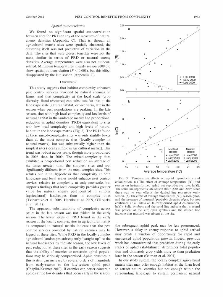
FIG. 3. Temperature effects on aphid reproduction andcolonization. (a) The effect of average temperature (8C) andseason on ln-transformed aphid net reproductive rate, ln(R).The solid line represents late season (both 2008 and 2009, sincethere was no year effect); the dashed line represents earlyseason. (b) The effect of average temperature (8C), season, year,and the presence of mustard (probably Brassica nigra, but notconfirmed at all sites) on ln-transformed aphid colonization,ln(C ). Solid symbols and the solid line indicate that mustardwas present at the site; open symbols and the dashed lineindicate that mustard was absent at the site.

October 2012 1943PEST CONTROL BENEFITS FROM COMPLEXITY

enemy populations. The three-year data, when examined

week-to-week instead of averaged over the growing

season, show that locally complex agricultural matrix

sites typically do not reach syrphid densities similar to

natural matrix sites until much later in the season, if at

all (Appendix D; also Chaplin-Kramer 2010). In

addition, though only five observations of natural

enemies (primarily lacewings and spiders) were recorded

in our point-estimates during the early season, all five

occurred at natural matrix sites. Enemies arriving on the

scene later in the season are likely drawn to the

substantial prey resource in the fields, but may just be

skimming off the top, rather than providing true top-

down control. The effective delivery of pest control

services may rely in large part on the presence of a

healthy natural enemy community on the farm early in

the season, such as might occur with nearby over-

wintering populations, when aphid populations are

small and not increasing as rapidly, and when natural

enemies have the best chance of preventing populations

from growing. In fact, other work in this system has

shown that early-season aphid colonization allows

natural enemies to establish sufficient population levels

to contain aphid population levels below economic

thresholds (Nieto et al. 2006). While PRD does not

correspond to the absolute densities that determine

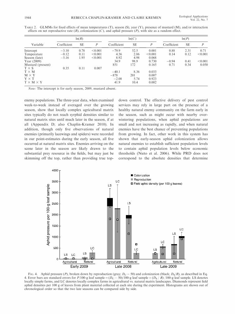
TABLE 2. GLMMs for fixed effects of mean temperatures (T), season (S), year (Y), presence of mustard (M), and/or interactioneffects on net reproductive rate (R), colonization (C ), and aphid pressure (P), with site as a random effect.

Variable

ln(R) ln(C ) ln(P)

Coefficient SE P Coefficient SE P Coefficient SE P

Intercept �3.10 0.78 ,0.001 �79.9 52.5 0.001 0.88 2.31 0.71Temperature �0.12 0.11 ,0.001 4.56 2.86 ,0.001 0.14 0.12 ,0.001Season (late) �5.16 1.95 ,0.001 8.92 4.98 0.068Year (2009) 34.9 98.9 0.730 �0.94 0.41 ,0.001Mustard (present) 851 172 0.165 0.71 0.34 0.050T 3 S 0.35 0.11 0.007T 3 M �40.1 8.36 0.033M 3 Y �878 201 0.007Y 3 T �2.08 5.74 0.923T 3 M 3 Y 41.9 10.4 0.002

Note: The intercept is for early season, 2009, mustard absent.

FIG. 4. Aphid pressure (P), broken down by reproduction (gray; DC� 50) and colonization (black; DS/R), as described in Eq.4. Error bars are standard errors for P/100-g leaf sample¼ (DC� 50)/100-g leaf sampleþ (DS / R) /100-g leaf sample. LS denoteslocally simple farms, and LC denotes locally complex farms in agricultural vs. natural matrix landscapes. Diamonds represent fieldaphid densities per 100 g of leaves from plant material collected at each site during the experiment. Histograms are shown out ofchronological order so that the two late seasons can be compared side by side.

REBECCA CHAPLIN-KRAMER AND CLAIRE KREMEN1944 Ecological ApplicationsVol. 22, No. 7

FIG. 5. (a, c, e) The effect of landscape matrix and local complexity on natural enemy densities, paired with (b, d, f ) the effectsof natural enemy densities on proportional reduction of aphid densities, PRD. (a) Point-estimate ln-transformed syrphid densitiesper 100-g leaf sample (mean 6 SE) collected at each site during the experiment, increasing in complexity from left to right: locallysimple agricultural matrix, locally complex agricultural matrix, locally simple natural matrix, locally complex natural matrix. (b)Natural log (ln) transformed PRD vs. point-estimate ln-transformed syrphid densities per 100-g leaf sample. Early season 2009 isnot shown, as no syrphids were detected using this method. (c) Three-year average ln-transformed syrphid densities per plant (fromdata collected 2006–2008) in habitats of increasing complexity left to right), with plant masses typically ranging from 100 to 1500 gover the growing season. (d) Natural log (ln) transformed PRD vs. three-year average ln-transformed syrphid densities per plant.(e) Three-year average ln-transformed pooled densities of other (non-syrphid) natural enemies per plant in habitats of increasingcomplexity (left to right). (f ) Natural log (ln) transformed PRD vs. three-year average ln-transformed pooled densities of other(non-syrphid) natural enemies per plant.

October 2012 1945PEST CONTROL BENEFITS FROM COMPLEXITY

economic thresholds, the reduction in aphid densities

provided by natural enemies associated with greater

habitat complexity can be considered in terms of

avoided damages. The exclusion of natural enemies

has resulted in a 31% lower harvest rate for broccoli in

this region (Nieto et al. 2006).

Aphid distributions in this system may be determined

by many factors other than top-down control. Densities

of aphids in the fields were correlated with aphid

pressure in the cages, but landscape or local complexity

did not significantly impact aphid densities in either field

or cage (Fig. 4), despite the strong effect of complexity

on PRD. However, this snapshot approach of measur-

ing aphid densities fails to capture subtler effects of

landscape complexity on population growth trajectories

that may be more indicative of the level of pest control

that is occurring (Chaplin-Kramer et al. 2011b), and

higher temporal resolution data in this system suggest

that aphid densities do decline with landscape complex-

ity (R. Chaplin-Kramer, P. de Valpine, N. J. Mills, and

C. Kremen, unpublished manuscript). Other factors

beyond habitat complexity must be considered in order

to understand and anticipate pest pressure and the

contribution natural enemies can make to effective pest

control in agricultural settings. Warmer temperatures

enhance aphid reproductive rates (Fig. 3a), and could

potentially overwhelm the control an enemy community

might otherwise provide in cooler conditions. Indeed,

temperature was seen to be the overriding factor

determining aphid densities in the field and aphid

pressure in the experimental cages in this system.

Colonization, the other component of aphid pressure,

was influenced by alternate host plant presence (Fig. 3b),

suggesting that the specific composition of habitat on

and around the farm is important. Colonization is also

presumably influenced by prevailing wind patterns, since

aphids are not strong fliers (Dixon and Howard 1986).

In areas of high recruitment, a constant supply of aphids

replenishing those lost to predation may mask the pest

control service that is simultaneously being provided by

natural enemies.

Management for ecosystem services requires a knowl-

edge of the scales at which management efforts will

produce the greatest benefit (Kremen 2005). While the

landscape scale appears to be more important to pest

reduction in this system than the local scale, growers

typically have more control over their local habitat than

the surrounding landscape. On-farm management,

especially the creation of habitat for natural enemies

via hedgerows or insectary strips and the exclusion of

alternate host plants for pests, can benefit pest control in

certain circumstances. However, such management may

not be sufficient to constrain pest populations below

economic thresholds, and farmers may need to employ

other methods to achieve the desired level of control

(Andow 1990, Zehnder et al. 2007). Meanwhile, efforts

to protect or restore larger tracts of habitat at the

landscape scale must carefully consider which types of

habitat to promote, wherever possible selecting habitat

that maximizes resources for beneficial insects while

minimizing its potential to serve as a refuge for pests.

Restoration goals often focus on other aspects of

conservation than the impact of habitat on pest control

services, but conservation projects may gain more

traction when all potential ecosystem services accruing

TABLE 3. GLMMs for fixed effects of landscape matrix (La) and/or local complexity (Lo) on ln-transformed point-estimate late-season field syrphid abundance (Sp), ln-transformed mean syrphid abundance from three-year survey data (Sm), and ln-transformed mean abundance of pooled data for all other natural enemies (E), with site as a random effect.

Variable

Sp Sm E

Coefficient SE P Coefficient SE P Coefficient SE P

Intercept (agricultural-simple) 0.62 0.31 0.08 1.71 0.47 0.003 0.47 0.17 0.01La (natural) 1.83 0.38 0.002 1.32 0.50 0.02 0.38 0.17 0.06Lo (complex) 0.66 0.39 0.13 0.70 0.50 0.21

TABLE 4. GLMMs for fixed effects of natural enemy densities, season, year, and/or interactions effects on proportional reductionof aphid densities,�ln(PRD), with site as a random effect.

Variable

�ln(PRD) ; Sp. . . �ln(PRD) ; Sm. . . �ln(PRD) ; E. . .

Coefficient SE P Coefficient SE P Coefficient SE P

Intercept (2008/late) 0.58 0.37 0.14 �0.55 0.67 0.42 �1.17 0.84 0.18Enemy 0.74 0.22 0.05 1.19 0.29 0.004 4.56 1.15 0.01Y (2009) 0.16 0.40 0.08S (late) 0.85 0.83 0.09 1.55 0.92 0.08Enemy 3 Y �0.56 0.24 0.06Enemy 3 S �0.75 0.35 0.05 �3.33 1.26 0.02

Notes: Measurements for enemy densities include point-estimate late-season ln-transformed field syrphid abundance (Sp), ln-transformed mean syrphid abundance from three-year survey data (Sm), and ln(mean abundance) of pooled data for all othernatural enemies (E). In the headings, ellipses indicate that the full equation includes the heading variable (Sp, Sm, or E) plus thevariables listed in column 1 (see Table 2 for definitions).

REBECCA CHAPLIN-KRAMER AND CLAIRE KREMEN1946 Ecological ApplicationsVol. 22, No. 7

from their implementation are considered (Nelson et al.

2009).

The important message for growers and land manag-

ers is that habitat complexity improves pest control

services at both local and landscape scales. However,

pest control services, as defined here, are not the same as

pest control. Certain habitats around farm sites may

promote pest population growth by influencing micro-

climate or providing resources to pests. Pest infestations

on diverse farms and/or in natural landscapes may still

occur without indicating a failure of complexity to

enhance natural enemy suppression of pests; to the

contrary, the pest problem could be much worse without

it. In many cases, considering other variables contrib-

uting to pest distributions in addition to top-down

factors will be necessary in order to achieve effective

natural pest control.

ACKNOWLEDGMENTS

We are grateful to Earthbound Farms, Route 1 Organics,Pinnacle Organics, Tanimura and Antle, Crown Packing,Swanton Berry Farm, ALBA farms, and the UCSC andUSDA experimental farms for their participation in thisproject, and Bill Chaney and Hugh Smith for their invaluableadvice. Shalene Jha, Nick Mills, Perry de Valpine, and twoanonymous reviewers provided helpful comments on themanuscript. We thank the Environmental Systems ResearchInstitute for their gift of ArcGIS software to the BerkeleyNatural History Museums, and we benefited from the supportand services of UC–Berkeley’s Geospatial Innovation Facility(gif.berkeley.edu). Financial support came from the EnvironFoundation, the Organic Farming Research Foundation, theUSDA’s Western Sustainable Agriculture Research and Edu-cation program, and the University of California–Berkeley; R.Chaplin-Kramer was supported by a National Science Foun-dation graduate fellowship.

LITERATURE CITED

Andow, D. A. 1990. Population dynamics of an insectherbivore in simple and diverse habitats. Ecology 71:1006–1017.

Bianchi, F. J. J. A., C. J. H. Booij, and T. Tscharntke. 2006.Sustainable pest regulation in agricultural landscapes: areview on landscape composition, biodiversity and naturalpest control. Proceedings of the Royal Society B 273:1715–1727.

Bianchi, F. J. J. A., P. W. Goedhart, and J. M. Baveco. 2008.Enhanced pest control in cabbage crops near forest in TheNetherlands. Landscape Ecology 23:595–602.

Chaplin-Kramer, R. 2010. The landscape ecology of pestcontrol services: cabbage aphid-syrphid trophic dynamicson California’s Central Coast. Dissertation. University ofCalifornia, Berkeley, California, USA.

Chaplin-Kramer, R., D. Kliebenstein, A. Chiem, E. Morrill, N.Mills, and C. Kremen. 2011a. Chemically-mediated tritrophicinteractions: opposing effects of glucosinolates on a specialistherbivore and its predators. Journal of Applied Ecology48:880–887.

Chaplin-Kramer, R., M. E. O’Rourke, E. J. Blitzer, and C.Kremen. 2011b. A meta-analysis of crop pest and naturalenemy response to landscape complexity. Ecology Letters14:922–932.

Clough, Y., A. Kruess, D. Kleijn, and T. Tscharntke. 2005.Spider diversity in cereal fields: comparing factors at local,landscape and regional scales. Journal of Biogeography32:2007–2014.

Collier, T., and R. Van Steenwyk. 2004. A critical evaluation ofaugmentative biological control. Biological Control 31:245–256.

den Belder, E., J. Elderson, W. Van Den Brink, and G.Schelling. 2002. Effect of woodlots on thrips density in leekfields: a landscape analysis. Agriculture, Ecosystems andEnvironment 91:139–145.

Dixon, A. F. G. 1977. Aphid ecology: life cycles, polymor-phism, and population regulation. Annual Review ofEcology and Systematics 8:329–353.

Dixon, A. F. G., and M. T. Howard. 1986. Dispersal in aphids,a problem in resource allocation. Pages 145–151 in W.Danthanarayana, editor. Insect flight dispersal and migra-tion. Springer, New York, New York, USA.

Elliott, N. C., R. W. Kieckhefer, J. H. Lee, and B. W. French.1998. Influence of within-field and landscape factors on aphidpredator populations in wheat. Landscape Ecology 14:239–252.

Eskenazi, B., A. R. Marks, A. Bradman, K. Harley, D. B. Barr,C. Johnson, N. Morga, and N. P. Jewell. 2007. Organophos-phate pesticide exposure and neurodevelopment in youngMexican-American children. Environmental Health Perspec-tives 115:792–798.

Fiedler, A. K., D. A. Landis, and S. D. Wratten. 2008.Maximizing ecosystem services from conservation biologicalcontrol: the role of habitat management. Biological Control45:254–271.

Gardiner, M. M., D. A. Landis, C. Gratton, C. D. DiFonzo,M. O’Neal, J. M. Chacon, M. T. Wayo, N. P. Schmidt, E. E.Mueller, and G. E. Heimpel. 2009. Landscape diversityenhances biological control of an introduced crop pest in thenorth-central USA. Ecological Applications 19:143–154.

Gueorguieva, R., and J. H. Krystal. 2004. Move over ANOVA:progress in analyzing repeated-measures data and itsreflection in papers published in the archives of generalpsychiatry. Archives of General Psychiatry 61:310–317.

Gurr, G. M., H. F. van Emden, and S. Wratten. 1998. Habitatmanipulation and natural enemy efficiency: implications forcontrol of pests. Pages 155–183 in P. Barbosa, editor.Conservation biological control. Academic Press, San Diego,California, USA.

Haenke, S., B. Scheid, M. Schaefer, T. Tscharntke, and C.Thies. 2009. Increasing syrphid fly diversity and density insown flower strips within simple vs. complex landscapes.Journal of Applied Ecology 46:1106–1114.

Hughes, R. D. 1963. Population dynamics of the cabbage aphidBrevicoryne brassicae (L.). Journal of Animal Ecology32:393–424.

Kremen, C. 2005. Managing ecosystem services: what do weneed to know about their ecology? Ecology Letters 8:468–479.

Kremen, C., N. M. Williams, R. L. Bugg, J. P. Fay, and R. W.Thorp. 2004. The area requirements of an ecosystem service:crop pollination by native bee communities in California.Ecology Letters 7:1109–1119.

Landis, D. A., S. D. Wratten, and G. M. Gurr. 2000. Habitatmanagement to conserve natural enemies of arthropod pestsin agriculture. Annual Review of Entomology 45:175–201.

Letourneau, D. K., and S. G. Bothwell. 2008. Comparison oforganic and conventional farms: challenging ecologists tomake biodiversity functional. Frontiers in Ecology and theEnvironment 6:430–438.

Letourneau, D. K., and B. Goldstein. 2001. Pest damage andarthropod community structure in organic vs. conventionaltomato production in California. Journal of Applied Ecology38:557–570.

Lichstein, J. W., T. R. Simons, S. A. Shriner, and K. E.Franzreb. 2002. Spatial autocorrelation and autoregressivemodels in ecology. Ecological Monographs 72:445–463.

Nelson, E., et al. 2009. Modeling multiple ecosystem services,biodiversity conservation, commodity production, and trade-

October 2012 1947PEST CONTROL BENEFITS FROM COMPLEXITY

offs at landscape scales. Frontiers in Ecology and theEnvironment 7:4–11.

Nieto, D. J., C. Shennan, W. H. Settle, R. O. Malley, S. Bros,and J. Y. Honda. 2006. How natural enemies and cabbageaphid (Brevicoryne brassicae L.) population dynamics affectorganic broccoli harvest. Environmental Entomology 35:94–101.

O’Rourke, M. E., K. Rienzo-Stack, and A. G. Power. 2011. Amulti-scale, landscape approach to predicting insect popula-tions in agroecosystems. Ecological Applications 21:1782–1791.

Ostman, O., B. Ekbom, and J. Bengtsson. 2001. Landscapeheterogeneity and farming practice influence biologicalcontrol. Basic and Applied Ecology 2:365–371.

Pimentel, D., H. Acquay, M. Biltonen, P. Rice, M. Silva, J.Nelson, V. Lipner, A. Horowitz, and M. D. Amore. 1992.Environmental and economic costs of pesticide use. BioSci-ence 42:750–760.

Prado, E., and W. Tjallingii. 2007. Behavioral evidence for localreduction of aphid-induced resistance. Journal of InsectScience 7:48.

Ruttan, V. W. 1999. The transition to agricultural sustainabil-ity. Proceedings of the National Academy of Sciences USA96:5960–5967.

Settle, W. H., H. Ariawan, E. T. Astuti, W. Cahyana, A. L.Hakim, D. Hindayana, A. S. Lestari, Pajarningsih, andSartanto. 1996. Managing tropical rice pests through

conservation of generalist natural enemies and alternativeprey. Ecology 77:1975–1988.

Stiling, P. 1993. Why do natural enemies fail in classicalbiological control programs? American Entomologist 39:31–37.

Thies, C., and T. Tscharntke. 1999. Landscape structure andbiological control in agroecosystems. Science 285:893–895.

Tscharntke, T., A. M. Klein, A. Kruess, I. Steffan-Dewenter,and C. Thies. 2005. Landscape perspectives on agriculturalintensification and biodiversity—ecosystem service manage-ment. Ecology Letters 8:857–874.

UC IPM. 2008. UC IPM pest management guidelines: tomato.UC ANR Publication 3470. http://www.ipm.ucdavis.edu/PMG/r783900111.html#REFERENCE

van Emden, H. 1963. A field technique for comparing theintensity of mortality factors acting on the cabbage aphid,Brevicoryne brassicae (L.) (Hem: Aphididae), in differentareas of a crop. Entomologia Experimentalis et Applicata6:53–62.

Werling, B. P., and C. Gratton. 2008. Influence of field marginsand landscape context on ground beetle diversity inWisconsin (USA) potato fields. Agriculture, Ecosystemsand Environment 128:104–108.

Zehnder, G., G. M. Gurr, S. Kuhne, M. R. Wade, S. D.Wratten, and E. Wyss. 2007. Arthropod pest management inorganic crops. Annual Review of Entomology 52:57–80.

SUPPLEMENTAL MATERIAL

Appendix A

A photograph showing the design of experimental cages (Ecological Archives A022-104-A1).

Appendix B

Effects of year, season, landscape complexity, and local complexity on maximum, mean, and minimum temperatures (EcologicalArchives A022-104-A2).

Appendix C

Moran’s index to test for spatial autocorrelation of sites for variables that responded significantly to landscape complexity(Ecological Archives A022-104-A3).

Appendix D

Average weekly syrphid larvae densities from 2006 to 2008 (Ecological Archives A022-104-A4).

REBECCA CHAPLIN-KRAMER AND CLAIRE KREMEN1948 Ecological ApplicationsVol. 22, No. 7