190
MathCode C++ Peter Fritzson MathCode C++ Release 1.4 July 2009
| Date post: | 27-Jul-2018 |
| Category: |
Documents |
| Upload: | trinhthuan |
| View: | 221 times |
| Download: | 0 times |

MathCode C++
Peter Fritzson
MathCode C++ Release 1.4
July 2009

MathCode is a trademark of MathCore Engineering AB.
Mathematica is a trademark of Wolfram Research Inc.
Matlab is a trademark of MathWorks Inc.
Windows95/98/NT/XP, Visual C++, MS-DOS, Developer Studio and MFC are trademarks of Microsoft corporation.
UNIX is a trademark of The Open Group.
Solaris is a trademark of Sun Microsystems Inc.
Other trademarks belong to their respective owners.
For further information, visit http://www.mathcore.com or email [email protected]
For support, email [email protected]
Copyright © 1998-2009 MathCore Engineering AB
All rights reserved. Reproduction or use of editorial or pictorial content in any manner is prohib-ited without explicit permission provided in writing. No patent liability is assumed with respect to the use of the information contained herein. While every precaution has been taken in the prepa-ration of this book, the publisher assumes no responsibility for errors or omissions. Neither is any liability assumed for damages resulting from the use of the information contained herein.
First edition, 2006
Preface
Mathematica is a comprehensive numeric and symbolic programming system with applica-tions in a wide range of areas. The MathCode code generation system presented in this book adds very high performance, connectivity to external applications and easy-to-use ma-trix arithmetic to this system. The combined Mathematica & MathCode system becomes a very powerful environment that supports both design, prototyping, programming and docu-mentation.
MathCode makes it possible to develop prototypes in the interactive Mathematicaenvironment which can be automatically translated to fast production code in C++ or Fortran90 and, if necessary, linked to external applications. Generated code is typically about 1000 times faster than basic Mathematica code, and it is often close to 100 times faster than code generated by the standard Mathematica Compile. Both stand-alone code and connected code can be produced. Connectivity from Mathematica to C, C++, Fortran77 or Fortran90 code is obtained by automatically generating MathLink code for calling generated code and external applications.
Callbacks from external applications to Mathematica can be generated automatically. Generation of stand-alone external code is supported. Symbolic Mathematica code can be translated provided that the final result of symbolic operations are arithmetic expressions.
To summarize, MathCode opens up completely new possibilities for cost-effective development of high-performance computational applications in the highly productive Mathematica environment.
Several people have contributed to particular subject matters within this book and MathCode. Johan Gunnarsson contributed to the general design in a number of places, most of the chapter on array slice operations as well as their implementation in Mathematica, parts of the high-level code transformations, and several notebook examples. Vadim Engelson implemented parts of the low-level code generator and helped with the external functions and trouble shooting chapter, as well as contributed to the MathCode array package and the implementation of external functions and callbacks. Pontus Lidman made most of the index to this book, most of the installation instructions, and helped with editing and minor corrections. Mats Jirstrand gave useful comments regarding the manuscript.
Yelena Turetskaya checked the most recent version of this book. Many other people have read the manuscript and given valuable comments. Thank you!
The MathCode system is inspired by the code-generation facilities in an earlier research prototype called ObjectMath, intended for object-oriented mathematical modeling and efficient code generation. This prototype was developed between 1990-96 at the Programming Environments Laboratory, Department of Computer and Information Science, Linköping University, with contributions from myself, Dag Fritzson, Niclas Andersson, Vadim Engelson, Johan Herber, Patrik Hägglund, Lars Viklund, Rickard Westman, and Lars Willför. Vadim Engelson has maintained and further developed the system, including the most recent version. The development of ObjectMath was strongly influenced by the fruitful cooperation with SKF, where the system was used for applications in bearing modeling and simulation.
Linköping, Sweden, 2004 Peter Fritzson

How to Read this Book
This section gives a short reader’s guide to the contents of this book. Before starting to read, note that installation instructions for MathCode are distributed together wth installation me-dia, See distribution CD and read the instructions before you start software installation. MathCode FAQ (frequently asked questions) as well as latest software updates are availi-able at www. mathcore.com
Chapter 1 gives a quick introduction to the basic facilities in MathCode, including a small “hands-on” example for the reader to try out. This introduction is enough to be able to use MathCode on simple applications.
Chapter 2 provides more comprehensive examples of translation. This includes both symbolically expanded code and numeric code, how to organize your code into packages to be translated by MathCode, as well as performance measurements of compiled code and comparison with Matlab. After reading chapter 1 and looking at these examples you should be able to use MathCode on medium-sized applications, even though it is advisable to read appropriate additional chapters for more complete information.
Chapter 3 covers the convenient array, vector, and matrix operations made available in Mathematica by MathCode. This chapter should be read by anyone interested in array and matrix operations.
Chapter 4 explains the notions of type system and static/dynamic typing. The need for typing and some of the design decisions in MathCode are motivated. Reading this chapter is not necessary in order to use MathCode but gives useful background information.
Additional information concerning declarations of constants, variables, arrays, and functions is given in Chapter 5, which is more detailed than the quick overview in Chapter 1.
Chapter 6 presents an overview of data structure allocation and declaration, with special emphasis on arrays. Related array issues, such as array indexing, are also covered.
Chapter 7 gives a comprehensive description of commands and options for code generation, compilation, linking with compiled object modules and/or external libraries, and building executables.
Chapter 8 presents the MathCode call interface to external code written in languages such as C, C++, Fortran77 and Fortran90, as well as the callback mechanism to

Mathematica from code written in these languages.(Mathcode C++ only)Chapter 9 presents system information, MathCode distribution structure and installation
instructions.Chapter 10 explains the MathCode translation structure and gives hints on
troubleshooting. The typed subset of Mathematica which can be compiled by MathCode is defined in
Appendix A. Use this appendix as a short reference guide.

7
Contents
1 Quick Tour of MathCode 17
1.1 Introduction . . . . . . . . . . . . . . . . . . . . . . . . . . . . . . . . . . . . . . . . . 171.2 Short Example . . . . . . . . . . . . . . . . . . . . . . . . . . . . . . . . . . . . . . . 171.3 Using the MathCode System . . . . . . . . . . . . . . . . . . . . . . . . . . . . . 20
1.3.1 Code Generating Phase . . . . . . . . . . . . . . . . . . . . . . . . . . . 211.3.2 Building Phase . . . . . . . . . . . . . . . . . . . . . . . . . . . . . . . . . 211.3.3 Executing Phase . . . . . . . . . . . . . . . . . . . . . . . . . . . . . . . . 21
1.4 MathCode Type System . . . . . . . . . . . . . . . . . . . . . . . . . . . . . . . . 211.4.1 Dual Type System . . . . . . . . . . . . . . . . . . . . . . . . . . . . . . . 221.4.2 Basic Types . . . . . . . . . . . . . . . . . . . . . . . . . . . . . . . . . . . 221.4.3 Declarations . . . . . . . . . . . . . . . . . . . . . . . . . . . . . . . . . . . 231.4.4 Function Signatures . . . . . . . . . . . . . . . . . . . . . . . . . . . . . . 231.4.5 Arrays and Lists . . . . . . . . . . . . . . . . . . . . . . . . . . . . . . . . 25
Basic Array Static Type Definition . . . . . . . . . . . . . . . . . . 25Examples . . . . . . . . . . . . . . . . . . . . . . . . . . . . . . . . . . . . . 25Unspecified Dimension Sizes . . . . . . . . . . . . . . . . . . . . . . . 26Named Dimension Placeholders . . . . . . . . . . . . . . . . . . . . . 26Array Sizes in Function Signatures . . . . . . . . . . . . . . . . . . 26Dimension Sizes of Array Parameters . . . . . . . . . . . . . . . . . 27Initialization of Arrays in Declarations . . . . . . . . . . . . . . . 27
1.5 Compilation to C++ code . . . . . . . . . . . . . . . . . . . . . . . . . . . . . . . 271.5.1 Calling the Code Generator . . . . . . . . . . . . . . . . . . . . . . . . 28
CompilePackage . . . . . . . . . . . . . . . . . . . . . . . . . . . . . . . . 28SetCompilationOptions . . . . . . . . . . . . . . . . . . . . . . . . . . . 28
8
Compiling Different Items . . . . . . . . . . . . . . . . . . . . . . . . . 291.5.2 Building . . . . . . . . . . . . . . . . . . . . . . . . . . . . . . . . . . . . . . 30
MakeBinary . . . . . . . . . . . . . . . . . . . . . . . . . . . . . . . . . . . . 30BuildCode . . . . . . . . . . . . . . . . . . . . . . . . . . . . . . . . . . . . . 30
1.5.3 Installing . . . . . . . . . . . . . . . . . . . . . . . . . . . . . . . . . . . . . . 30InstallCode . . . . . . . . . . . . . . . . . . . . . . . . . . . . . . . . . . . . 30
1.5.4 Executing . . . . . . . . . . . . . . . . . . . . . . . . . . . . . . . . . . . . . 311.5.5 Uninstalling . . . . . . . . . . . . . . . . . . . . . . . . . . . . . . . . . . . . 31
1.6 Matrix Operations . . . . . . . . . . . . . . . . . . . . . . . . . . . . . . . . . . . . . 311.7 Implementing Missing Mathematica Functions . . . . . . . . . . . . . . . . 32
1.7.1 Callbacks to Mathematica . . . . . . . . . . . . . . . . . . . . . . . . . 331.7.2 An Example system.nb Notebook . . . . . . . . . . . . . . . . . . . . 33
Initialization Needed to use MathCode . . . . . . . . . . . . . . . . 33Package Header . . . . . . . . . . . . . . . . . . . . . . . . . . . . . . . . . 33Public Exported Global Symbols . . . . . . . . . . . . . . . . . . . . 33Private Implementation Section . . . . . . . . . . . . . . . . . . . . . 34Compiling . . . . . . . . . . . . . . . . . . . . . . . . . . . . . . . . . . . . . 34Building . . . . . . . . . . . . . . . . . . . . . . . . . . . . . . . . . . . . . . 35Install and Test . . . . . . . . . . . . . . . . . . . . . . . . . . . . . . . . . 35
1.8 Interfacing With External Libraries . . . . . . . . . . . . . . . . . . . . . . . . 351.8.1 Linking with External Libraries . . . . . . . . . . . . . . . . . . . . . 35
1.9 MathCode Limitations . . . . . . . . . . . . . . . . . . . . . . . . . . . . . . . . . . 36
2 Getting Started by Examples 37
2.1 Compilation and Code Generation . . . . . . . . . . . . . . . . . . . . . . . . . 382.2 Two Modes of Code Generation . . . . . . . . . . . . . . . . . . . . . . . . . . . 382.3 The SinSurface Application Example . . . . . . . . . . . . . . . . . . . . . . . 40
2.3.1 Introduction . . . . . . . . . . . . . . . . . . . . . . . . . . . . . . . . . . . . 402.3.2 Initialization . . . . . . . . . . . . . . . . . . . . . . . . . . . . . . . . . . . 40
Check Current Directory . . . . . . . . . . . . . . . . . . . . . . . . . . 402.3.3 Start of the SinSurface Package . . . . . . . . . . . . . . . . . . . . . 41
Exported Symbols . . . . . . . . . . . . . . . . . . . . . . . . . . . . . . . 41
9
Setting Compilation Options . . . . . . . . . . . . . . . . . . . . . . . 422.3.4 The Body of the SinSurface Package . . . . . . . . . . . . . . . . . 422.3.5 Functions and Declarations to be Translated to C++ . . . . . . 42
Global Variables . . . . . . . . . . . . . . . . . . . . . . . . . . . . . . . . 42sin, cos . . . . . . . . . . . . . . . . . . . . . . . . . . . . . . . . . . . . . . . 42arcTan . . . . . . . . . . . . . . . . . . . . . . . . . . . . . . . . . . . . . . . 43sinFun2 . . . . . . . . . . . . . . . . . . . . . . . . . . . . . . . . . . . . . . . 43calcPlot . . . . . . . . . . . . . . . . . . . . . . . . . . . . . . . . . . . . . . . 44End of SinSurface Package . . . . . . . . . . . . . . . . . . . . . . . . 44
2.3.6 Execution . . . . . . . . . . . . . . . . . . . . . . . . . . . . . . . . . . . . . 44Mathematica Evaluation . . . . . . . . . . . . . . . . . . . . . . . . . . 44Using Mathematica Standard Compile[] . . . . . . . . . . . . . . . 45
2.3.7 Using the MathCode Code Generator . . . . . . . . . . . . . . . . . 45The Generated C++ Code . . . . . . . . . . . . . . . . . . . . . . . . . 46Compiling and Linking the C++ Code . . . . . . . . . . . . . . . . 50Installing and Connecting to Mathematica . . . . . . . . . . . . . 50Execution of generated C++ Code . . . . . . . . . . . . . . . . . . . 51
2.3.8 Performance Comparison . . . . . . . . . . . . . . . . . . . . . . . . . . 512.4 The Gauss Application Example . . . . . . . . . . . . . . . . . . . . . . . . . . 53
2.4.1 The Gauss Package . . . . . . . . . . . . . . . . . . . . . . . . . . . . . . 53Initialization of the Package . . . . . . . . . . . . . . . . . . . . . . . 53Start the Package . . . . . . . . . . . . . . . . . . . . . . . . . . . . . . . . 53Define Exported Symbols . . . . . . . . . . . . . . . . . . . . . . . . . 53Define the Functions and Variables . . . . . . . . . . . . . . . . . . 53GaussSolveArrayslice . . . . . . . . . . . . . . . . . . . . . . . . . . . . 54GaussSolveForLoops . . . . . . . . . . . . . . . . . . . . . . . . . . . . . 56The Compiled GaussSolveForLoops function, using Compile[]
58End of the Gauss Package . . . . . . . . . . . . . . . . . . . . . . . . . 60
2.4.2 Executing the Interpreted Version in Mathematica . . . . . . . 60Run GaussSolveArrayslice . . . . . . . . . . . . . . . . . . . . . . . . . 60Run the For-loop Version . . . . . . . . . . . . . . . . . . . . . . . . . 60

10
2.4.3 Generation of C++ code . . . . . . . . . . . . . . . . . . . . . . . . . . . 60The Produced C++ Code for Gauss . . . . . . . . . . . . . . . . . . . 61
2.4.4 Building the Executable . . . . . . . . . . . . . . . . . . . . . . . . . . . 682.4.5 Installing Compiled Code . . . . . . . . . . . . . . . . . . . . . . . . . . 682.4.6 Prepare for Execution . . . . . . . . . . . . . . . . . . . . . . . . . . . . . 682.4.7 External Execution . . . . . . . . . . . . . . . . . . . . . . . . . . . . . . . 68
External Execution of Array Slice Version . . . . . . . . . . . . . 68External Array Slice Version, MathLink in each Iteration . . 69External Execution of For-Loop Version . . . . . . . . . . . . . . . 69External For-loop Version, MathLink in each Iteration . . . . 69External Array Slice Version with InlineFlag and No Range 69External For-Loop Version with InlineFlag and No Range . . 70Internal Execution of LinearSolve as a Comparison . . . . . . . 70Internal execution of Compiled version . . . . . . . . . . . . . . . . 70
2.4.8 Cleanup . . . . . . . . . . . . . . . . . . . . . . . . . . . . . . . . . . . . . . . 70
3 Matrix and Vector Operations 73
3.1 Examples of Array Operations . . . . . . . . . . . . . . . . . . . . . . . . . . . . 733.2 Index Range Notation . . . . . . . . . . . . . . . . . . . . . . . . . . . . . . . . . . 74
3.2.1 Omitting End of Index Range . . . . . . . . . . . . . . . . . . . . . . . 743.2.2 Omitting Start of Index Range . . . . . . . . . . . . . . . . . . . . . . 753.2.3 Omitting Both Start and End of a Range . . . . . . . . . . . . . . . 75
3.3 Vectors Versus Rows and Columns . . . . . . . . . . . . . . . . . . . . . . . . 763.3.1 One-dimensional Vectors . . . . . . . . . . . . . . . . . . . . . . . . . . 763.3.2 Row Vectors . . . . . . . . . . . . . . . . . . . . . . . . . . . . . . . . . . . 763.3.3 Column Vectors . . . . . . . . . . . . . . . . . . . . . . . . . . . . . . . . . 76
3.4 Extracting or Assigning Vectors From Vectors . . . . . . . . . . . . . . . . 773.5 Extracting Vectors From Matrices . . . . . . . . . . . . . . . . . . . . . . . . . 78
3.5.1 Extracting One-dimensional Vectors . . . . . . . . . . . . . . . . . . 783.5.2 Extracting Vectors as Submatrices of Shape 1×n or n×1 . . . 78
3.6 Assigning Vectors to Rows or Columns of Matrices . . . . . . . . . . . . 793.7 Extracting and Assigning Arbitrary Submatrices . . . . . . . . . . . . . . 80
11
3.8 Promotion of Scalars to Vectors or Matrices . . . . . . . . . . . . . . . . . 813.9 An Example Matrix Function . . . . . . . . . . . . . . . . . . . . . . . . . . . . 823.10 Current Limitations . . . . . . . . . . . . . . . . . . . . . . . . . . . . . . . . . . . 82
4 Rationale for Type Declarations in Mathematica 83
4.1 Why Type Declarations? . . . . . . . . . . . . . . . . . . . . . . . . . . . . . . . . 834.2 Types for Code Generation . . . . . . . . . . . . . . . . . . . . . . . . . . . . . . 844.3 The Need for Type Checking . . . . . . . . . . . . . . . . . . . . . . . . . . . . 844.4 Types for Object Oriented Simulation Modeling . . . . . . . . . . . . . . 854.5 Introducing Declarations in Mathematica . . . . . . . . . . . . . . . . . . . 854.6 Declarations in Mathematica Packages . . . . . . . . . . . . . . . . . . . . . 864.7 Basic Types . . . . . . . . . . . . . . . . . . . . . . . . . . . . . . . . . . . . . . . . . 864.8 Dual Type System . . . . . . . . . . . . . . . . . . . . . . . . . . . . . . . . . . . . 874.9 Typed Function Declarations . . . . . . . . . . . . . . . . . . . . . . . . . . . . 87
4.9.1 Type Arguments to the Mathematica Compile Function . . . 894.10 Typed Declarations . . . . . . . . . . . . . . . . . . . . . . . . . . . . . . . . . . . . 89
5 More on Typing and Declarations 91
5.1 Basic Types . . . . . . . . . . . . . . . . . . . . . . . . . . . . . . . . . . . . . . . . . 915.2 Declarations . . . . . . . . . . . . . . . . . . . . . . . . . . . . . . . . . . . . . . . . . 92
5.2.1 Variable Declarations . . . . . . . . . . . . . . . . . . . . . . . . . . . . 925.2.2 Constant Declarations . . . . . . . . . . . . . . . . . . . . . . . . . . . . 93
5.3 Type Constructors and Data Constructors . . . . . . . . . . . . . . . . . . . 945.3.1 List Structures and Array Types . . . . . . . . . . . . . . . . . . . . . 945.3.2 Array Type Constructors . . . . . . . . . . . . . . . . . . . . . . . . . . 945.3.3 Data Constructors . . . . . . . . . . . . . . . . . . . . . . . . . . . . . . . 95
5.4 Array Variable Declarations . . . . . . . . . . . . . . . . . . . . . . . . . . . . . 955.4.1 Declaring Multiple Array Variables . . . . . . . . . . . . . . . . . . 95
5.5 Functions . . . . . . . . . . . . . . . . . . . . . . . . . . . . . . . . . . . . . . . . . . . 965.5.1 Functions with No Input Parameters . . . . . . . . . . . . . . . . . . 965.5.2 Functions with Multiple Return Values . . . . . . . . . . . . . . . 97
12
5.5.3 Functions Returning Arrays . . . . . . . . . . . . . . . . . . . . . . . . 975.5.4 Functions with No Return Value . . . . . . . . . . . . . . . . . . . . . 975.5.5 Functions with Local Variables . . . . . . . . . . . . . . . . . . . . . 985.5.6 Structure of a Small Example Package with Typed Functions 995.5.7 External Functions . . . . . . . . . . . . . . . . . . . . . . . . . . . . . . 100
6 Data Allocation and Initialization 101
6.1 When Should Allocation and Initialization be Performed? . . . . . . 1026.1.1 Initialization of Global Variables . . . . . . . . . . . . . . . . . . . 102
Local Variables . . . . . . . . . . . . . . . . . . . . . . . . . . . . . . . . 1036.1.2 Execution Parameters . . . . . . . . . . . . . . . . . . . . . . . . . . . . 103
6.2 Array Allocation and Initialization . . . . . . . . . . . . . . . . . . . . . . . . 1036.2.1 Array Usage and Representation in Mathematica . . . . . . . . 1046.2.2 Array Initialization by Promoted Scalar Values . . . . . . . . . 104
Initialization of Runtime Sized Arrays . . . . . . . . . . . . . . . 105Allocation Without Initialization . . . . . . . . . . . . . . . . . . . 105General Initializers . . . . . . . . . . . . . . . . . . . . . . . . . . . . . 106Unspecified Dimension Sizes . . . . . . . . . . . . . . . . . . . . . . 107
6.2.3 Summary of Array Dimension Specification . . . . . . . . . . . 108Array Dimensions for Function Parameters and Results . . . 108Array Dimensions for Declared Variables . . . . . . . . . . . . . 108
6.3 Array Index Bounds . . . . . . . . . . . . . . . . . . . . . . . . . . . . . . . . . . 1096.3.1 Array Index Lower Bounds . . . . . . . . . . . . . . . . . . . . . . . . 1096.3.2 Dimension Sizes and Upper Index Bounds . . . . . . . . . . . . 1106.3.3 Declaring Local Arrays with Variable Dimension Sizes . . . 110
Negative Indices . . . . . . . . . . . . . . . . . . . . . . . . . . . . . . . 1116.4 Array Constructor Functions . . . . . . . . . . . . . . . . . . . . . . . . . . . . 112
6.4.1 Array Dimension Size Functions . . . . . . . . . . . . . . . . . . . 113
7 Compilation and Code Generation 115
7.1 Overall System Structure . . . . . . . . . . . . . . . . . . . . . . . . . . . . . . . 116
13
7.2 Compilation and Code Generation Aspects . . . . . . . . . . . . . . . . . 1167.2.1 Target Code Type . . . . . . . . . . . . . . . . . . . . . . . . . . . . . . 1167.2.2 Evaluation of Symbolic Operations . . . . . . . . . . . . . . . . . 1177.2.3 Integration . . . . . . . . . . . . . . . . . . . . . . . . . . . . . . . . . . . 117
7.3 Invoking the Code Generator . . . . . . . . . . . . . . . . . . . . . . . . . . . 1187.3.1 CompilePackage[]—the Primary Code Generation Function 118
CompilePackage[packagename] . . . . . . . . . . . . . . . . . . . . 118Different Items to be Compiled . . . . . . . . . . . . . . . . . . . . 119
7.3.2 Optional Parameters to Control Code Generation . . . . . . . 119SetCompilationOptions . . . . . . . . . . . . . . . . . . . . . . . . . . 119Priority of Parameter Settings . . . . . . . . . . . . . . . . . . . . . 120Option EvaluateFunctions . . . . . . . . . . . . . . . . . . . . . . . . 120Option UnCompiledFunctions . . . . . . . . . . . . . . . . . . . . . 120Option DisabledMathLinkFunctions . . . . . . . . . . . . . . . . . 120Option CallBackFunctions . . . . . . . . . . . . . . . . . . . . . . . . 121Option MainFileAndFunction . . . . . . . . . . . . . . . . . . . . . . 121Option ExternalLanguage . . . . . . . . . . . . . . . . . . . . . . . . 121Option NeedsExternalLibrary . . . . . . . . . . . . . . . . . . . . . 121Option NeedsExternalObjectModule . . . . . . . . . . . . . . . . . 122Option InlineFlag . . . . . . . . . . . . . . . . . . . . . . . . . . . . . . 122Option RangeCheckFlag . . . . . . . . . . . . . . . . . . . . . . . . . 122Option MacroRules . . . . . . . . . . . . . . . . . . . . . . . . . . . . . 122Option DebugFlag . . . . . . . . . . . . . . . . . . . . . . . . . . . . . . 123Option Language . . . . . . . . . . . . . . . . . . . . . . . . . . . . . . . 123Option Compiler . . . . . . . . . . . . . . . . . . . . . . . . . . . . . . . 123Option CompilerOptions . . . . . . . . . . . . . . . . . . . . . . . . . 124Option LinkerOptions . . . . . . . . . . . . . . . . . . . . . . . . . . . 124Option MathCodeMakeFile . . . . . . . . . . . . . . . . . . . . . . . 124
7.4 Standard Layout of a Package to be Compiled . . . . . . . . . . . . . . . 1257.5 Code Generation of Symbolically Evaluated Expressions . . . . . . . 126
Common Subexpression Elimination . . . . . . . . . . . . . . . . 126A Short Example . . . . . . . . . . . . . . . . . . . . . . . . . . . . . . . 126
14
7.6 Building Executables . . . . . . . . . . . . . . . . . . . . . . . . . . . . . . . . . . 1277.6.1 MakeBinary["packagename"] . . . . . . . . . . . . . . . . . . . . . . 128
Setting Compilation Options for the C++ Compiler . . . . . . 128Controlling Type of Binary Executable . . . . . . . . . . . . . . . 128Linking with External Object Code . . . . . . . . . . . . . . . . . . 129
7.6.2 BuildCode["packagename"] . . . . . . . . . . . . . . . . . . . . . . . 1307.7 Integration . . . . . . . . . . . . . . . . . . . . . . . . . . . . . . . . . . . . . . . . . 130
7.7.1 Calling Compiled Generated Code via MathLink . . . . . . . . 130Code Storage Places . . . . . . . . . . . . . . . . . . . . . . . . . . . . . 132
7.7.2 Integration of External Libraries and Software Modules . . 1327.7.3 Callbacks to Mathematica . . . . . . . . . . . . . . . . . . . . . . . . 132
Errors in Callbacks . . . . . . . . . . . . . . . . . . . . . . . . . . . . . . 133Placement of Generated Callback Stub Functions . . . . . . . 134
7.8 Providing Missing Mathematica Functions . . . . . . . . . . . . . . . . . . 1347.8.1 The system Package . . . . . . . . . . . . . . . . . . . . . . . . . . . . . 135
7.9 Code Compilation from Command Shell . . . . . . . . . . . . . . . . . . . 1357.9.1 Command Shell Compilation in Windows using make . . . . 1367.9.2 Command Shell Compilation in Windows using nmake . . . 1367.9.3 Command Shell Compilation in UNIX . . . . . . . . . . . . . . . 136
8 Interfacing to External Libraries 137
8.1 External Variables . . . . . . . . . . . . . . . . . . . . . . . . . . . . . . . . . . . . 1378.2 External Functions . . . . . . . . . . . . . . . . . . . . . . . . . . . . . . . . . . . 137
8.2.1 Data Transfer at Function Call . . . . . . . . . . . . . . . . . . . . . 1388.2.2 Mapping External Function Interfaces to Mathematica . . . 1398.2.3 ExternalFunction and ExternalProcedure Declarations . . . . 1398.2.4 Specification of External Function Language . . . . . . . . . . 1408.2.5 Examples . . . . . . . . . . . . . . . . . . . . . . . . . . . . . . . . . . . . . 141
External Input Parameters, no External Function Value . . . 141External Input Parameters, External Function Value . . . . . 141Default External Output Parameters, no Value . . . . . . . . . 142
8.2.6 Examples of Fortran and C functions . . . . . . . . . . . . . . . . 142
15
Named External Output Parameters, External Procedure . . 142Arbitrary Placement of External Output Parameters . . . . . 143External InOut/Reference Parameters, External Procedure 144
8.2.7 Calling External Fortran Library Functions . . . . . . . . . . . 1458.2.8 Passing Array Parameters to External Functions . . . . . . . . 146
Passing Array Parameters to External C++ Functions . . . . 146Passing Array Parameters to External Fortran77 Functions 147
8.3 Linking with External Object Code . . . . . . . . . . . . . . . . . . . . . . . 1508.4 Summary of Interfacing External Code . . . . . . . . . . . . . . . . . . . . 151
9 System and Installation Information 153
9.1 Files in the MathCode Distribution . . . . . . . . . . . . . . . . . . . . . . . 1539.2 System-specific installation information . . . . . . . . . . . . . . . . . . . 1549.3 Supported C++ Compilers . . . . . . . . . . . . . . . . . . . . . . . . . . . . . . 1549.4 ReadMe Information and Release Notes . . . . . . . . . . . . . . . . . . . 154
10 Trouble Shooting 155
10.1 Code Generation Phases . . . . . . . . . . . . . . . . . . . . . . . . . . . . . . . 15610.2 Error Categories . . . . . . . . . . . . . . . . . . . . . . . . . . . . . . . . . . . . . 156
10.2.1 Packaging Errors - Missing Functions . . . . . . . . . . . . . . . 15710.2.2 Syntactic Errors . . . . . . . . . . . . . . . . . . . . . . . . . . . . . . . 15710.2.3 Semantic Errors . . . . . . . . . . . . . . . . . . . . . . . . . . . . . . . . 15810.2.4 Errors During C++ Compilation and Linking . . . . . . . . . . 15910.2.5 Internal Code Generator Errors . . . . . . . . . . . . . . . . . . . . 15910.2.6 Long Compilation Times . . . . . . . . . . . . . . . . . . . . . . . . . 15910.2.7 Internal Errors During Execution of Generated Code . . . . 160
10.3 Appendix . . . . . . . . . . . . . . . . . . . . . . . . . . . . . . . . . . . . . . . . . . 160
A The Compilable Mathematica Subset 161
A.1 Operations not in the Compilable Subset . . . . . . . . . . . . . . . . . . . . 161A.2 Predefined Functions and Operators . . . . . . . . . . . . . . . . . . . . . . . 163
16
A.2.1 Statements and Value Expressions . . . . . . . . . . . . . . . . . . . 164A.2.2 Function Call . . . . . . . . . . . . . . . . . . . . . . . . . . . . . . . . . . . 164A.2.3 Function Definition . . . . . . . . . . . . . . . . . . . . . . . . . . . . . . 165A.2.4 Scope Constructs . . . . . . . . . . . . . . . . . . . . . . . . . . . . . . . . 165A.2.5 Control Statements . . . . . . . . . . . . . . . . . . . . . . . . . . . . . . . 166A.2.6 Mapping Operations . . . . . . . . . . . . . . . . . . . . . . . . . . . . . . 167A.2.7 Iterator Expressions . . . . . . . . . . . . . . . . . . . . . . . . . . . . . . 167A.2.8 Input/Output Operations . . . . . . . . . . . . . . . . . . . . . . . . . . . 168A.2.9 Standard Arithmetic and Logic Expressions . . . . . . . . . . . . 169A.2.10 Named Constants . . . . . . . . . . . . . . . . . . . . . . . . . . . . . . . . 173A.2.11 Assignment Expressions . . . . . . . . . . . . . . . . . . . . . . . . . . . 173A.2.12 Array Data Constructors . . . . . . . . . . . . . . . . . . . . . . . . . . . 174A.2.13 Array Data Manipulation . . . . . . . . . . . . . . . . . . . . . . . . . . 174A.2.14 Statisics and sorting functions . . . . . . . . . . . . . . . . . . . . . . 175A.2.15 Array Dimension Functions . . . . . . . . . . . . . . . . . . . . . . . . 176A.2.16 Array Indexing . . . . . . . . . . . . . . . . . . . . . . . . . . . . . . . . . 176A.2.17 Array Section Operations . . . . . . . . . . . . . . . . . . . . . . . . . . 177A.2.18 Other Expressions . . . . . . . . . . . . . . . . . . . . . . . . . . . . . . . 177
List . . . . . . . . . . . . . . . . . . . . . . . . . . . . . . . . . . . . . . . . . . 178Apply . . . . . . . . . . . . . . . . . . . . . . . . . . . . . . . . . . . . . . . . 178
A.2.19 Operators Which May Have Side-effects . . . . . . . . . . . . . . . 179A.3 Predefined Types . . . . . . . . . . . . . . . . . . . . . . . . . . . . . . . . . . . . . 179
A.3.1 Basic Types . . . . . . . . . . . . . . . . . . . . . . . . . . . . . . . . . . . . 180A.3.2 Array Type Constructors . . . . . . . . . . . . . . . . . . . . . . . . . . 180
A.4 Predefined Constants . . . . . . . . . . . . . . . . . . . . . . . . . . . . . . . . . . . 180
1.1 Introduction 17
Chapter 1 Quick Tour of MathCode
1.1 IntroductionMathCode is a Mathematica application package which includes the following:
• Translation of a subset of Mathematica to efficient C++ code• Type annotations compatible with standard Mathematica• Availability of Matlab-like matrix operations on array sections both in Mathematica and
in compiled code
• Transparent calling of compiled executable code via MathLink or stand-alone execution• Transparent calling of external library functions in C, C++, or Fortran77• Transparent callbacks from external executables to Mathematica functions
The performance of compiled generated C++ code is often approximately 1000 times better than standard interpreted Mathematica, and often 100 times better than code compiled using the internal Mathematica compiler.
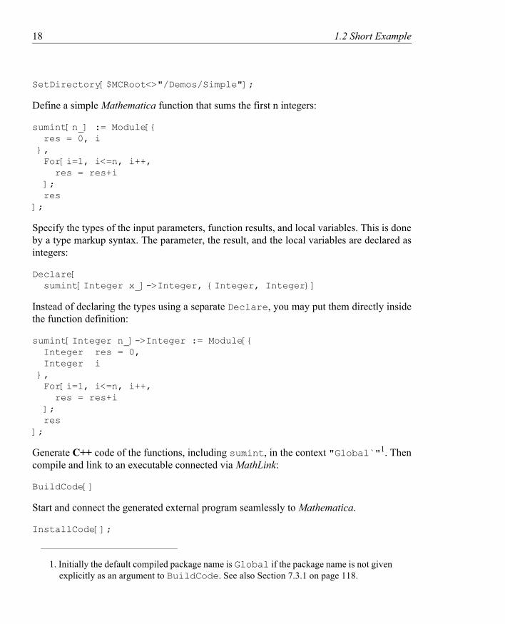
1.2 Short ExampleThe following short example shows one way of using the MathCode system. It is recom-mended that you try it yourself! You must have a C++ compiler installed on your system in order for the generated code to be executable.
The following command will load MathCode:
Needs["MathCode`"]
You might want to set the working directory to a subdirectory such as ".../Demos/Simple"under the MathCode root directory. Otherwise all files produced by MathCode will be writ-ten to the current directory.
18 1.2 Short Example
SetDirectory[$MCRoot<>"/Demos/Simple"];
Define a simple Mathematica function that sums the first n integers:
sumint[n_] := Module[{ res = 0, i }, For[i=1, i<=n, i++, res = res+i ]; res];
Specify the types of the input parameters, function results, and local variables. This is done by a type markup syntax. The parameter, the result, and the local variables are declared as integers:
Declare[ sumint[Integer x_]->Integer, {Integer, Integer}]
Instead of declaring the types using a separate Declare, you may put them directly inside the function definition:
sumint[Integer n_]->Integer := Module[{ Integer res = 0, Integer i }, For[i=1, i<=n, i++, res = res+i ]; res];
Generate C++ code of the functions, including sumint, in the context "Global`"1. Then compile and link to an executable connected via MathLink:
BuildCode[]
Start and connect the generated external program seamlessly to Mathematica.
InstallCode[];
1. Initially the default compiled package name is Global if the package name is not given explicitly as an argument to BuildCode. See also Section 7.3.1 on page 118.

1.2 Short Example 19
The external variant of sumint can now be called transparently in the same way as a func-tion inside Mathematica:
sumint[10000]
The result is:
50005000
Give the command to look at the generated C++ source file:
!!Global.cc
The generated source code, including an empty package initialization function:
#include "Global.h"#include <math.h>int Global_sumint( const int &n){ int res = 0; int i; i = 1; while (i <= n) { res = res+i; i = i+1; } return res;}
void Global_GlobalInit (){; }
Uninstall the external code and clean up the directory:
UnInstallCode[];
CleanMathCodeFiles[];Remove["Global`"];
20 1.3 Using the MathCode System
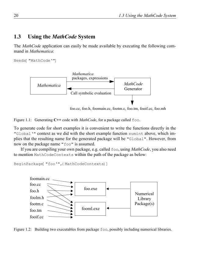
1.3 Using the MathCode SystemThe MathCode application can easily be made available by executing the following com-mand in Mathematica:
Needs["MathCode‘"]
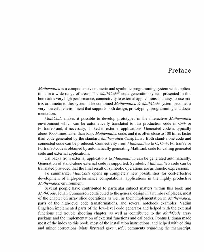
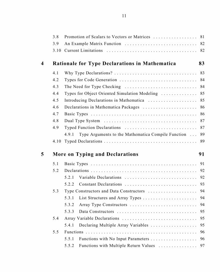
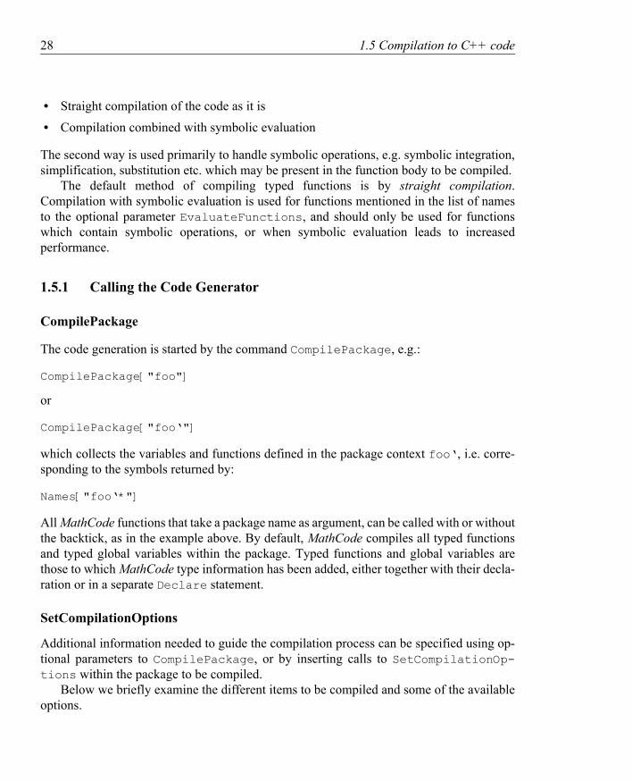
Mathematica MathCodeGenerator
Mathematicapackages, expressions
Call symbolic evaluation
foo.cc, foo.h, foomain.cc, footm.c, foo.tm, fooif.cc, foo.mh
Figure 1.1: Generating C++ code with MathCode, for a package called foo.
To generate code for short examples it is convenient to write the functions directly in the "Global‘" context as we did with the short example function sumint above, which im-plies that the resulting name for the generated package will be "Global". However, from now on the package name "foo" is assumed.
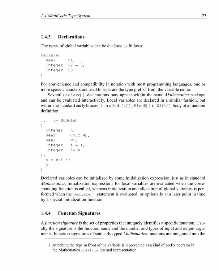
If you are compiling your own package, e.g. called foo, using MathCode, you also need to mention MathCodeContexts within the path of the package as below:
BeginPackage["foo‘",{MathCodeContexts}]
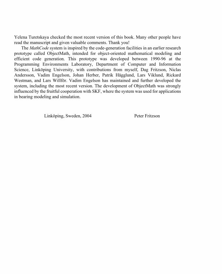
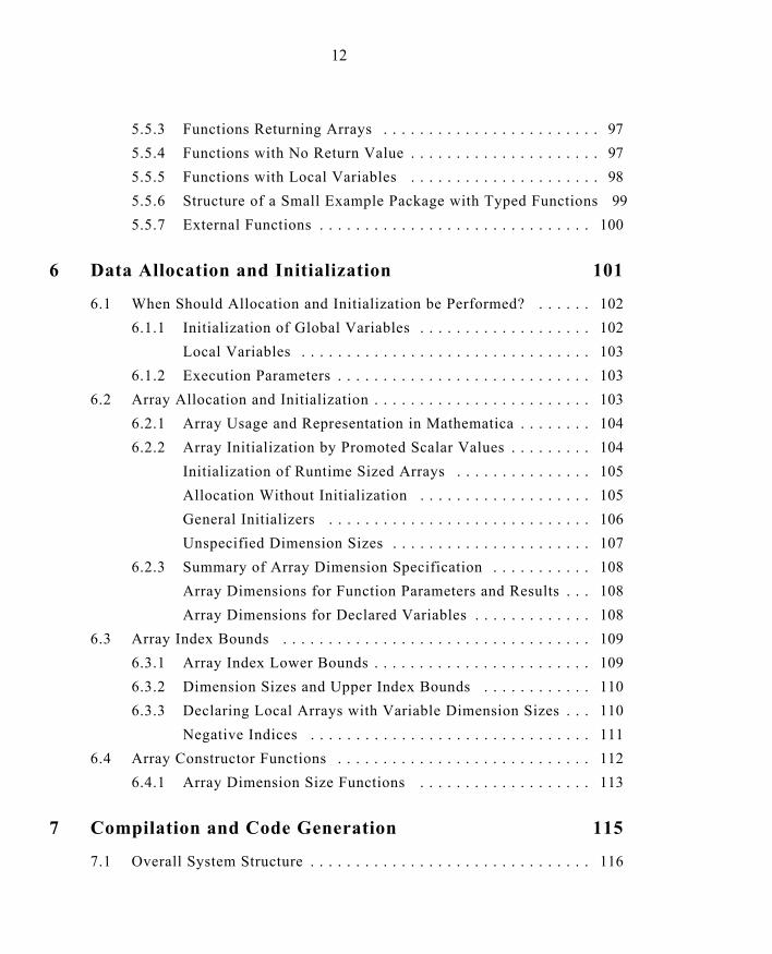
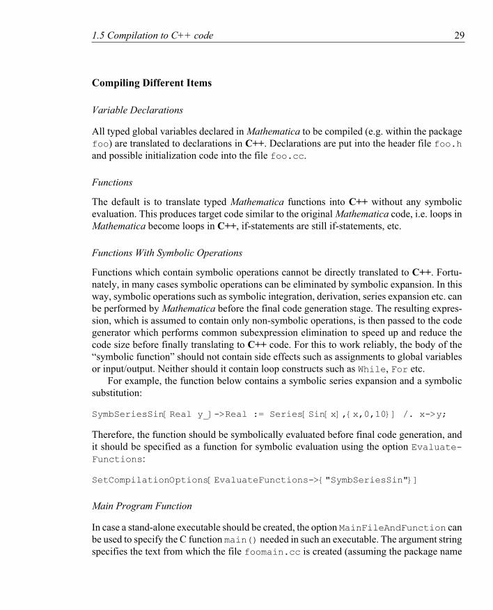
foo.exeNumerical
Package(s)fooml.exe
foo.ccfoo.h
foomain.cc
footm.cfoo.tm
Library
fooif.cc
foolm.h
Figure 1.2: Building two executables from package foo, possibly including numerical libraries.

1.4 MathCode Type System 21
1.3.1 Code Generating Phase
The MathCode code generator translates a Mathematica package, here called foo, to a cor-responding C++ source file, here called foo.cc. Additional files which are automatically produced are: the header file foo.h, the MathCode header file foo.mh, the MathLink re-lated files footm.c, foo.tm, and fooif.cc. These files enable transparent calling of the C++ versions of functions in foo from Mathematica, and foomain.cc which contains the function main needed when building a stand-alone executable for foo (Figure 1.3)
1.3.2 Building Phase
The generated file foo.cc created from the package foo together with the header file foo.h and additional files are compiled and linked into an executable: either foo.exe or fooml.exe. Numerical libraries may be included in the linking process by specifying in-clusion of external libraries (Figure 1.2).
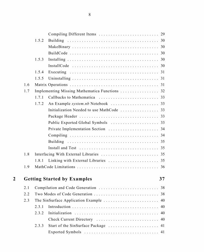
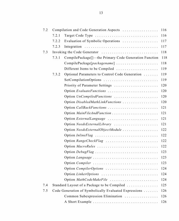
1.3.3 Executing Phase
The produced executable foo.exe1 can be used for stand-alone execution, whereas fooml.exe is used when transparent calling from Mathematica via MathLink of the com-piled C++ functions in fooml.exe is desired.
foo.exe
MathematicaNeeds["foo‘"]
fooml.exeMathLink
Figure 1.3: Executing compiled code. The executable foo.exe is used for stand-alone execution, whereas functions in fooml.exe are called interactively from Mathematica via MathLink.
1.4 MathCode Type SystemThe MathCode type system allows the user to associate static type information with Math-
1. The .exe extension is also used under Unix systems such as Solaris, Linux, etc.

22 1.4 MathCode Type System
ematica variables and functions. This information is needed in order to generate efficient code in strongly typed languages such as C++. Future versions of MathCode may support inference of some type information, but the current version requires specification of types for all variables and functions to be translated to C++.
1.4.1 Dual Type System
Standard Mathematica is dynamically typed; thus types may change during execution. For example a variable x may first be a symbol, next change into an expression and finally change into a real floating-point number during evaluation. In order to constrain dynamical-ly changing types at run-time, Mathematica provides pattern-matching constructs. For ex-ample: to only allow certain dynamic types of arguments when a function foo is called:
foo[x_Real, y_Integer] := ...
The function foo above can only be called with the first argument being a floating-point val-ue and the second an integer value. It cannot be called, for example, for variables which are still symbols, in which case the full expression is returned in unevaluated form.
On the other hand, in a static type system, one would like to express that a variable always has the static type Real even though it can be represented by a symbol, expression,or floating-point value. This is especially relevant for compiling to statically typed languages and for static type checking. Another need for static types is for user-defined types; for example a variable could have a static type Voltage even though it has a real value and would have matched the head Real in Mathematica.
Thus, to handle both needs we must a dual type system where we can express both dynamic and static types. We describe below how to declare static types as an extension of the existing dynamic type system in Mathematica.
1.4.2 Basic Types
The following basic types are supported by the current version of MathCode:
Integer, Real, Complex
The Real type corresponds to IEEE double precision floating point types in generated code. Support for the following additional basic types is not yet implemented (except for a rudi-mentary support for String and Boolean, as specified in Appendix A):
Boolean, String
1.4 MathCode Type System 23
1.4.3 Declarations
The types of global variables can be declared as follows:
Declare[ Real r1, Integer i2 = 3, Integer i3]
For convenience and compatibility in notation with most programming languages, one or more space characters are used to separate the type prefix1 from the variable name.
Several Declare[] declarations may appear within the same Mathematica packageand can be evaluated interactively. Local variables are declared in a similar fashion, but within the standard curly braces {} in a Module[], Block[] or With[] body of a function definition:
... := Module[{ Integer n, Real {y,z,w}, Real w2, Integer i = 1, Integer j= 0}, y = x+i+j; y]
Declared variables can be initialized by some initialization expression, just as in standard Mathematica. Initialization expressions for local variables are evaluated when the corre-sponding function is called, whereas initialization and allocation of global variables is per-formed when the Declare[] statement is evaluated, or optionally at a later point in time by a special initialization function.
1.4.4 Function Signatures
A function signature is the set of properties that uniquely identifies a specific function. Usu-ally the signature is the function name and the number and types of input and output argu-ments. Function signatures of statically typed Mathematica functions are integrated into the
1. Attaching the type in front of the variable is represented as a kind of prefix operator in the Mathematica FullForm internal representation.

24 1.4 MathCode Type System
function definitions, or can be provided in a separate Declare statement. The integration of function signatures into function definitions has been made possible by an extension of the standard := and -> operators. This does not change the behavior or performance of the Mathematica functions, when executed interpretively within Mathematica, and is thus com-pletely backwards compatible. The syntax has the following structure:
func[type1 x1, ..., typen xn]-> ftype := ...
Both static types and “dynamic types” can be specified, as in:
func[statictype x1_dynamictype1,...]->ftype := ...
The static type is only needed for code generation and does not influence the interpreted function definition within Mathematica, whereas the dynamic type is the traditional Mathe-matica pattern construct. For example, the function vfunc below will only match Realnumber arguments during execution in Mathematica:
vfunc[Voltage x1_Real,...]->Voltage := ...
Multiple function results are allowed and specified as such:
func[...]->{ftype1,...,ftypen} := ...
An example with one function result:
mytan[Real x_]->Real := Sin[x]/Cos[x];
An example with two results:
sinandcos[Real x_]->{Real,Real} := {Sin[x],Cos[x]};
When adding static type information to existing untyped Mathematica code, it may be more convenient to use the Declare method, as below, where the type information is provided separately:
Declare[mytan[Real x_]->Real];
mytan[x_]:=Sin[x]/Cos[x];
Apart from the function signatures, the types for the local variables are also needed in order to have full type information for a function. The keyword Declare[] can be used to specify both function signatures and types for local variables. The example below with a Declarestatement combined with a function declaration, e.g.:

1.4 MathCode Type System 25
Declare[myfunc[Integer x_, Real y_]->Real, {Real, Integer}]
myfunc[x_,y_] := Module[{myreal, myint}, ...
gives the same result as:
myfunc[Integer x_, Real y_]->Real := Module[{ Real myreal, Integer myint}, ...
1.4.5 Arrays and Lists
A key data structure in Mathematica is the list structure. Nested list structures are commonly used to represent matrices and other arrays. For example, a nested list {{2.1,3.1},{2.2,3.2}} is a two by two array of real numbers. The type of such (nest-ed) list structures can be specified by array type declarations, as long as they have a matrix-like shape and are homogenous, i.e. all elements have the same type.
It is interesting to note that Mathematica internally implements lists as arrays. This has the advantage of providing constant time indexing operations.
Basic Array Static Type Definition
Array types are represented by a type name parameterized by one or more dimension size specifiers:
type[size1,...,sizen]
Global array variables can be declared as below:
Declare[ type[size1,...,sizen] arr]
Examples
A type for a three dimensional array of real numbers:
Real[3,6,4]
Such an array could be declared as follows:
Declare[ Real[3,6,4] arr]
26 1.4 MathCode Type System
The sizes of array dimensions can be specified by values of integer variables, e.g. n and mbelow:
Integer[n,m]
Unspecified Dimension Sizes
Typically, the sizes of arrays passed as function parameters or returned from a function are not known until the function is executed. Such unspecified array-dimension sizes are indi-cated by the underscore (_) unnamed dimension placeholder or (ident_) named dimension placeholder. The actual values of dimension sizes may, however, be accessed later at runt-ime. This new use of underscore is only valid within array type specifiers, as shown below:
type[_,_]
Named Dimension Placeholders
Named dimension placeholders like n_ make it possible to express that the sizes of several dimensions are equal, as with square matrices. Such dimension placeholder names are local to the function where the type is used.
type[n_,n_]
This will give rise to a local variable n, which is initialized to the size of the array dimension as defined by the first occurrence of n. This variable can, for example, be used to declare local arrays of the same size.
Array Sizes in Function Signatures
Named dimension placeholders make it possible to express array-dimension size constraints in function signatures. For example, the following function signature is used for a matrix multiplication function, which multiplies two matrix parameters amat and bmat.
MatrixMult[Real[n_,k_] amat_, Real[k_,m_] bmat_] -> Real[n,m] := ...
This means that the dimension size parameters n, k, m are set to the dimension sizes of the input array arguments, and can be used in the function body or to specify output matrix type.No actual check is performed to verify that the second dimension of amat is equal to the first dimension of bmat
1.5 Compilation to C++ code 27
Dimension Sizes of Array Parameters
Finding the dimension sizes at run time, e.g. for a function array parameter mat, can be done simply by placing named dimension size placeholders in the input array type specifying those sizes. The placeholder variables can later be used for declaring the local array local-mat:
func[Real[n_,m_] mat_]->Real := Module[{ Real[n,m] localmat}, ...]
The sizes given for the output type are currently for documentation purposes only; no actual checking is performed.
Initialization of Arrays in Declarations
Matrices can be initialized by a constant matrix, or elementwise by a scalar. Elementwise initialization of a matrix by a scalar constant (general expressions currently not allowed) can be done, for example, as below for locally or globally declared variables:
Real[2,3] mat = 5.0
which gives mat the following contents:
{{5.,5.,5.}, {5.,5.,5.}}
Initialization by a constant matrix can be done as follows:
Real[3,3] mat2 = { {1., 2., 3.}, {2., 3., 4.}, {3., 4., 5.} }
1.5 Compilation to C++ codeMathCode provides facilities to compile statically typed Mathematica functions and vari-ables to C++ code. Functions always reside in some package (or to be more precise, always in some context). If no package has been specified by the user, the default package Globalis usually used. The compiler is invoked by calling CompilePackage. There are essentially two ways to compile functions:
28 1.5 Compilation to C++ code
• Straight compilation of the code as it is• Compilation combined with symbolic evaluation
The second way is used primarily to handle symbolic operations, e.g. symbolic integration, simplification, substitution etc. which may be present in the function body to be compiled.
The default method of compiling typed functions is by straight compilation. Compilation with symbolic evaluation is used for functions mentioned in the list of names to the optional parameter EvaluateFunctions, and should only be used for functions which contain symbolic operations, or when symbolic evaluation leads to increased performance.
1.5.1 Calling the Code Generator
CompilePackage
The code generation is started by the command CompilePackage, e.g.:
CompilePackage["foo"]
or
CompilePackage["foo‘"]
which collects the variables and functions defined in the package context foo‘, i.e. corre-sponding to the symbols returned by:
Names["foo‘*"]
All MathCode functions that take a package name as argument, can be called with or without the backtick, as in the example above. By default, MathCode compiles all typed functions and typed global variables within the package. Typed functions and global variables are those to which MathCode type information has been added, either together with their decla-ration or in a separate Declare statement.
SetCompilationOptions
Additional information needed to guide the compilation process can be specified using op-tional parameters to CompilePackage, or by inserting calls to SetCompilationOp-tions within the package to be compiled.
Below we briefly examine the different items to be compiled and some of the available options.
1.5 Compilation to C++ code 29
Compiling Different Items
Variable Declarations
All typed global variables declared in Mathematica to be compiled (e.g. within the package foo) are translated to declarations in C++. Declarations are put into the header file foo.hand possible initialization code into the file foo.cc.
Functions
The default is to translate typed Mathematica functions into C++ without any symbolic evaluation. This produces target code similar to the original Mathematica code, i.e. loops in Mathematica become loops in C++, if-statements are still if-statements, etc.
Functions With Symbolic Operations
Functions which contain symbolic operations cannot be directly translated to C++. Fortu-nately, in many cases symbolic operations can be eliminated by symbolic expansion. In this way, symbolic operations such as symbolic integration, derivation, series expansion etc. can be performed by Mathematica before the final code generation stage. The resulting expres-sion, which is assumed to contain only non-symbolic operations, is then passed to the code generator which performs common subexpression elimination to speed up and reduce the code size before finally translating to C++ code. For this to work reliably, the body of the “symbolic function” should not contain side effects such as assignments to global variables or input/output. Neither should it contain loop constructs such as While, For etc.
For example, the function below contains a symbolic series expansion and a symbolic substitution:
SymbSeriesSin[Real y_]->Real := Series[Sin[x],{x,0,10}] /. x->y;
Therefore, the function should be symbolically evaluated before final code generation, andit should be specified as a function for symbolic evaluation using the option Evaluate-Functions:
SetCompilationOptions[EvaluateFunctions->{"SymbSeriesSin"}]
Main Program Function
In case a stand-alone executable should be created, the option MainFileAndFunction can be used to specify the C function main() needed in such an executable. The argument string specifies the text from which the file foomain.cc is created (assuming the package name

30 1.5 Compilation to C++ code
is foo). In the example below the function f is called and the result is printed by the pro-gram.
SetCompilationOptions[MainFileAndFunction-> "int main(){return 0;}"]
1.5.2 Building
The building process compiles all produced C++ files and links them into an executable.
MakeBinary
MakeBinary["foo"]
The call MakeBinary["foo"] builds all the files for either the stand-alone version of the application (e.g. foo.exe), or for the interactively callable MathLink version (e.g. fooml.exe).
BuildCode
BuildCode["foo"]
The call BuildCode["foo"] calls CompilePackage["foo"] and then MakeBinary["foo"]. For example, a call to BuildCode["foo"] will make a complete code generation, compilation and linking of the Mathematica package “foo”. As mentioned earlier, the backtick is allowed as used in package context specifications in Mathematica:
BuildCode["foo`"]
1.5.3 Installing
For compiled functions to be directly callable from within Mathematica, the code must be installed.
InstallCode
The call:
InstallCode["foo"]
or, equivalently,

1.6 Matrix Operations 31
InstallCode["foo`"]
installs the binary fooml.exe into Mathematica. It first saves (in the Mathematica work-space, to be restored if uninstalled) the original interpreted functions and then creates func-tion definition stubs out of the compiled package in Mathematica. This enables the calling of compiled functions from within Mathematica via MathLink.
1.5.4 Executing
Functions in the compiled and installed package can be executed by standard function calls just like functions in any standard Mathematica package. If stand-alone execution is desired, simply run the created stand-alone executable (which does not have an ml suffix in its name).
1.5.5 Uninstalling
When the compiled code is no longer to be accessible and the MathLink connection is to be closed down, UninstallCode should be called:
UninstallCode["foo"]
This will restore the original interpreted version of the package, (called foo in the exam-ple).
1.6 Matrix OperationsIn many engineering applications, matrices and matrix manipulation are very common. The availability of an easy-to-use and short-handed notation for manipulating matrices is impor-tant for these application domains. Thus, we have extended the Part ([[ ]]) operation in Mathematica to fulfill this objective.
The current basic set of matrix operations consists of operations on array sections. The syntax is inspired by the syntax used by Matlab and Fortran 90, and is supported by the MathCode code generator for up to 4-dimensional arrays and within Mathematica for an arbitrary number of dimensions.
As an example, create a small matrix A containing indexed symbols of the form a[i,j]:
A=Table[a[i,j],{i,4},{j,5}]; A//MatrixForm
{ {a[1,1], a[1,2], a[1,3], a[1,4], a[1,5]}, {a[2,1], a[2,2], a[2,3], a[2,4], a[2,5]}, {a[3,1], a[3,2], a[3,3], a[3,4], a[3,5]},

32 1.7 Implementing Missing Mathematica Functions
{a[4,1], a[4,2], a[4,3], a[4,4], a[4,5]} }
Below we extract row 2 and 3, using the Matlab-style notation A[[2|3,_]]. Compared to the standard Matlab syntax A(2:3,:) we have made a Mathematica
compatible version by replacing colon as a binary range operator with vertical bar (|), and replacing colon as a placeholder for the whole range of a dimension with underscore (_).
A[[2|3,_]] // MatrixForm
{ {a[2,1], a[2,2], a[2,3], a[2,4], a[2,5]}, {a[3,1], a[3,2], a[3,3], a[3,4], a[3,5]} }
Extract all but the first two columns, using A[[_, 3|_]] which corresponds to standard Matlab syntax A(:,3:). The notation 3|_ here means the range from the 3rd to the last col-umn.
A[[_,3|_]]//MatrixForm
{{a[1,3], a[1,4], a[1,5]}, {a[2,3], a[2,4], a[2,5]}, {a[3,3], a[3,4], a[3,5]}, {a[4,3], a[4,4], a[4,5]} }
Assign values to a submatrix of A:
A[[2|3,2|3]] = {{1,2}, {3,4}};
A // MatrixForm
{ {a[1,1], a[1,2], a[1,3], a[1,4], a[1,5]}, {a[2,1], 1, 2, a[2,4], a[2,5]}, {a[3,1], 3, 4, a[3,4], a[3,5]}, {a[4,1], a[4,2], a[4,3], a[4,4], a[4,5]} }
1.7 Implementing Missing Mathematica FunctionsThe MathCode system directly supports translation of a set of basic Mathematica
functions and operations, as defined in Appendix A. There are still quite a number of standard Mathematica functions not yet included in this set.There are basically three ways to solve this problem: • Callback. Standard Mathematica functions can be made callable from external code, by
providing callback declarations. This is easy, but often gives slow execution due to
1.7 Implementing Missing Mathematica Functions 33
MathLink overhead and interpreted evaluation.• Re-implementation. Standard functions can be re-implemented by hand, or by using
available external implementations e.g. from a library. This process is simplified by the availability of the system package described in Section 1.7.2 below.
• User-defined macros. Functions can be defined by macros/replacement rules passed in the option MacroRules to CompilePackage. See “Option MacroRules” on page 122.
1.7.1 Callbacks to Mathematica
Mathematica functions can be called from outside Mathematica if they are made back call-able by adding the function to the list for the CallBackFunctions compilation option. For example, to be able call RotateLeft in Mathematica from generated code, execute:
SetCompilationOptions[CallBackFunctions->{RotateLeft}]
1.7.2 An Example system.nb Notebook
This particular notebook system.nb contains an example system package (note lower-case!) with an alternative implementation of the standard function RotateLeft, which ear-lier was not in the standard subset supported by the MathCode translator.
Initialization Needed to use MathCode
Needs["MathCode‘"]
Package Header
BeginPackage["system‘",{MathCodeContexts}]
Public Exported Global Symbols
Begin["system‘"];Off[General::shdw]
Introduce symbols that should be exported outside the package (there exist some other sym-bols in this package as well).system`RotateRight;

34 1.7 Implementing Missing Mathematica Functions
End Public Section
On[General::shdw] (* avoid shadowing messages from Mathematica *)End[];
Private Implementation Section
Begin["‘Private‘"];
Define implementations of the functions and variables.
RotateRight
Definition of RotateRight for integer vectors:RotateRight[ Integer[_] a_]->Integer[_] := Module[{ Integer m=Dimensions[a][[1]] }, Module[{ Integer[m] res }, res[[2|m]]=a[[1|m-1]]; res[[1]]=a[[m]]; res]];
End of Private Section
End[];
End of Package
EndPackage[];
Compiling
Compile the system package into C++ code:
CompilePackage["system"];
1.8 Interfacing With External Libraries 35
Building
Compile the C++ files to binaries and possibly link into an executable:
MakeBinary["system"];
Install and Test
InstallCode["system"];
RotateRight test example.
RotateRight[{1,2,3,4}]=={4, 1, 2, 3}]True
Note that the MathCode compiled version of system`RotateRight is executed (via MathLink) because it is earlier in the context path than the Mathematica built-in function RotateRight.
1.8 Interfacing With External LibrariesMathCode provides a mechanism for interface and call functions in external libraries and object modules which have been implemented in languages like Fortran, C, or C++.
Such functions need to be declared either ExternalFunction or ExternalProcedure, as in the Fortran subroutine fooext below, which has two input parameters and two output parameters. It has no function value and therefore is declared as ExternalProcedure instead of the more common ExternalFunction:
fooext[Real x_,Integer y_]->{Real, Real}:= ExternalProcedure[x, y, Output u1, Output u2, ExternalLanguage->"Fortran"];
1.8.1 Linking with External Libraries
The object code of external libraries needs to be linked with the generated code to make ex-ternal functions callable. Additional parameters can be supplied to MakeBinary for this purpose:
MakeBinary[NeedsExternalLibrary->{"extlib1", "extlib2"}, NeedsExternalObjectModule->{"file3"} ]
36 1.9 MathCode Limitations
Note that the object module named file3 in the above example would correspond e.g. to the object module named file3.obj under Windows95, or file3.o under Unix.
Alternatively, and usually more conveniently, options like NeedsExternalLibraryor NeedsExternalModule can be set by inserting calls to SetCompilationOptionsinto the package which needs to call the external functions, like in the package foo below:
BeginPackage["foo‘"]....SetCompilationOptions[ NeedsExternalLibrary ->{"extlib1", "extlib2"}, NeedsExternalObjectModule ->{"file3"}]...Begin["‘Private‘"]...End[]EndPackage[]
1.9 MathCode LimitationsThe main limitation of MathCode is of course that it cannot compile the full Mathematicalanguage. The compilable subset is defined in Appendix A. This subset will grow in future releases of MathCode, but will never include the full Mathematica language since that would entail a complete reimplementation of most of Mathematica.

1.9 MathCode Limitations 37
Chapter 2 Getting Started by Examples
The purpose of this chapter is to walk through some aspects of the MathCode system by showing complete application examples in order to help the user become acquainted with some of the type and code generation facilities. Recall that a very simple example of the use of MathCode has already been presented in Section 1.2 at the beginning of Chapter 1. The two examples in this chapter are slightly more advanced, showing the use of packages, sym-bolic expansion and array slices.
The following applications will be presented below:
• SinSurface, which computes and plots a Sin-like surface function on a 2D grid, using symbolic series expansion to create the symbolic expression which is the body of the surface function.
• Gauss, which solves a linear equation system by a textbook Gauss elimination algorithm, programmed using both for-loops and Matlab-like array slice matrix operations.
Additional examples can be found in the Demos directory of the MathCode distribution.The performance of the generated code is measured for the presented applications. The
performance figures shown have been obtained for Mathematica 5.0 for Windows. You should re-run these examples to obtain the correct performance figures for your platform; when running MathCode compiled applications it is particularly the speedup figures which vary between platforms.
The below descriptions of the SinSurface and Gauss applications are valid for execution under Sun Solaris on Sun Sparc workstations, Linux, and Windows95/98/NT/2000/XP/..., which are the currently supported platforms for code generation at the time of writing.
Other facilities, such as type declarations and array slice operations, work on all Mathematica supported platforms.
In order to run the system, there must be a valid Mathematica license on your computer. Also, you must have installed the MathCode system. See installation description in Chapter 9.
38 2.1 Compilation and Code Generation
2.1 Compilation and Code GenerationAs briefly mentioned in the introductory overview chapter, there are several options con-cerning the compilation and code-generation facilities provided by MathCode for translation of typed Mathematica code:
• Target code. Specifies which type of code should be produced. Currently, only C++ or Fortran90 code generation is supported, depending on whether MathCode C++ or MathCode F90 is installed on your computer.
• Execution integration. The compiled code can either be directly callable from within Mathematica, or simply be placed in an external file.
• Symbolic expansion. The Mathematica code may contain symbolic operations which should be evaluated and expanded in conjunction with code generation.
These options are explained in more detail in Chapter 7 which covers code generation. In this chapter we present a few small application examples which illustrate some of these as-pects.
To use typed declarations and code-generation facilities for functions and data structures in your own package, you always need to refer to the MathCode application by evaluating a Needs statement:
Needs["MathCode‘"]
In order to invoke code-generation functions from within your package, you also need to in-clude the MathCode contexts in the search path of your package, as below:
BeginPackage["myPackage‘",{MathCodeContexts,...}]
2.2 Two Modes of Code GenerationThe first example application is a rather contrived small Mathematica program called Sin-Surface, which is designed to illustrate the two basic modes of the code generator: compila-tion without symbolic evaluation, which is default, and compilation preceded by symbolic expansion, which is indicated by setting the option EvaluateFunctions (see Section 2.3.5).
• Standard code generation. This is the default for generating procedural code from a typed Mathematica function. The function body is translated, e.g. to C++, as it is, without applying any symbolic transformations. Such a function may only contain non-symbolic operations, typically numeric computations over arrays and scalars. When translating to external code, e.g. in C++, emitted code will be rather close to the original
2.2 Two Modes of Code Generation 39
Mathematica code in structure.• Code generation preceded by symbolic evaluation. This is used to generate code from a
function that may contain symbolic operations, e.g. series expansion, symbolic integration, symbolic derivation, etc. It is not useful to perform such symbolic operations in languages like C++ or Fortran90, so they are therefore performed in Mathematica before the final translation.
The symbolic operations result in expressions that should contain only non-symbolic, typically numeric operations. This is typically the case since Mathematicaalways evaluates as far as possible. Thus, the function body is expanded (and simplified) into a usually huge symbolic expression before being transformed into C++ code, for example. The result is rather unrecognizable compared to the original Mathematicafunction since both symbolic expansion and optimizations such as common subexpression elimination have been performed.
The following two sections present the actual application examples.
40 2.3 The SinSurface Application Example
2.3 The SinSurface Application ExampleBelow we describe the SinSurface program example. It is structured as a standard Mathe-matica package within a notebook file SinSurface.nb. The actual computation is per-formed by the functions calcPlot, sinFun2 and their help functions.
The two functions calcPlot and sinFun2 in the SinSurface package will be translated to C++ together with the declaration of the global array xyMatrix.• The array xyMatrix represents a 21x21 grid on which the numeric function sinFun2
will be computed.• The function calcPlot accepts four arguments which are coordinates that describe a
square in the x-y plane, and one counter (iter) to make the function repeat the computation as many times as necessary for measuring execution time. For each point on a 21x21 grid in that square, the numeric function sinFun2 is called to compute a value that is stored as a matrix element in the matrix representing the grid.
• The function sinFun2 computes essentially the same values as Sin[x+y], but in a more complicated manner. This function uses a rather large expression obtained through conversion of the arguments into polar coordinates (through arcTan) and then uses series expansion of both Sin and Cos in 10 terms. The resulting large symbolic expression (more than a page) becomes the body of sinFun2, and is then used as input to CompilePackage[] with the EvaluateFunction option (see Section 7.5) to generate efficient C++ code.
2.3.1 Introduction
The SinSurface example application computes a function (here sinFun2) over a 2-D grid. The function values are first stored in the matrix xyMatrix before being plotted. The exe-cution of compiled C++ code for the function sinFun2 is approximately 1000 times faster than evaluating the same function interpretively within Mathematica.
To run this example, start Mathematica, open the notebook file “SinSurface.nb”, and either evaluate it cell by cell or all at once.
2.3.2 Initialization
Check Current Directory
Check the current directory, since a number of files will be placed there during the code-generation process. This particular example shows directories from a computer with the Windows platform.

2.3 The SinSurface Application Example 41
Directory[]
"C:\MathCode\Demos\SinSurface\"
You might want to place the directory somewhere where all generated files are put, e.g. the directory below, or another location.
SetDirectory["C:\MathCode\Demos\SinSurface\"]"C:\MathCode\Demos\SinSurface\"
2.3.3 Start of the SinSurface Package
First give a Needs statement, to make sure that the MathCode application is loaded:
Needs["MathCode‘"]
The SinSurface package starts in the usual way by a BeginPackage declaration which references other packages. The MathCodeContexts variable is needed in order to call the code-generation related functions.
BeginPackage["SinSurface‘", {MathCodeContexts}]; Clear["SinSurface‘*"];
Exported Symbols
Define possibly exported symbols. Even though it is not necessary here, we enclose these names within a Begin["SinSurface‘"] ... End[] type of “context bracket”, since this can be put into a cell in the notebook and conveniently re-evaluated (only this cell!) if new names are added to the list below.
Begin["SinSurface‘"] xyMatrix; calcPlot; sinFun1; sinFun2; arcTan; sin; cos; plot; cplus; plotfile;End[]
42 2.3 The SinSurface Application Example
Setting Compilation Options
This defines how the functions and variables in the SinSurface package should be compiled to C++. By default, all typed variables and functions are compiled. However, the compila-tion process can be controlled in a more detailed manner by giving compilation options to CompilePackage or via SetCompilationOptions. For example, in this package the function sinFun2 should be symbolically evaluated before being translated to code since it contains symbolic operations; the functions sin, cos, and arcTan should not be compiled at all since they are expanded within the body of sinFun2. The remaining typed function, calcPlot, will be compiled in the normal way.
SetCompilationOptions[ EvaluateFunctions->{sinFun2}, UnCompiledFunctions->{sin,cos,arcTan}, MainFileAndFunction->""]
2.3.4 The Body of the SinSurface Package
Begin with the implementation section of the SinSurface package, where functions are de-fined. This is usually private to avoid accidental name shadowing due to identical local vari-ables in several packages.
Begin["SinSurface‘Private‘"];
2.3.5 Functions and Declarations to be Translated to C++
Global Variables
Declare public global variables and private package-global variables:
Declare[ Real[21,21] xyMatrix ];
sin, cos
Taylor-expanded sin and cos functions called by sinFun2. In the normal order of eval-uation of function Sin[ ] the actual parameter is replaced, Sin[ ] is evaluated and series expansion is performed. To reorder this sequence of operations, z must be substituted with x after the series expansion.
2.3 The SinSurface Application Example 43
sin[Real x_ ]->Real := Normal[Series[Sin[z], {z,0,10}]] /. z -> x ;cos[Real x_ ]->Real := Normal[Series[Cos[z], {z,0,10}]] /. z -> x ;
arcTan
Conversion of grid point to an angle, called by sinFun2.
arcTan[Real x_, Real y_]->Real := ( If[x < 0, Pi, 0] + If[ x == 0, Sign[y]*Pi/2, ArcTan[y/x] ] );
sinFun2
The function sinFun2 is the function to be computed and plotted, called by calcPlot. It provides a more complicated and computationally heavier way (series expansion) to calcu-late approximately the same result as Sin[x+y]. This gives an example of a combination of symbolic and numeric operations as well as a rather standard mix of arithmetic opera-tions. The expanded symbolic expression which comprises the body of SinFun2 is between 1 and 2 pages long when printed.
Note that the types of local variables to sinFun2 need not be declared since setting theEvaluateFunctions option will make the whole function body symbolically expanded before translation to C++ code.
Note also that in order for a function to be symbolically expanded before final code generation it should be without side effects, e.g. no assignment to global variables or input/output. This is because the relative order between these actions when executing the code often changes when the symbolic expression is created and later rearranged and optimized by the code generator.
sinFun2[Real x_, Real y_]->Real := Block[ { Real {r,xx,yy} }, r = Sqrt[x^2+y^2]; xx = r*cos[arcTan[x,y]]; yy = r*sin[arcTan[x,y]]; sin[xx+yy] ];
44 2.3 The SinSurface Application Example
calcPlot
The function calcPlot calculates data for a plot of sinFun2 over a 21x21 grid, which is returned as a 21×21 array.
calcPlot[Real xmin_, Real xmax_, Real ymin_, Real ymax_, Integer iter_] -> Real[21,21] := Module[{ Integer n = 20, Real {x,y}, Integer {i,j,count} }, For[count=1,count<=iter,count=count+1, For[i=1, i<=(n+1), i=i+1, For[j=1, j<=(n+1), j=j+1,
x = xmin+(xmax-xmin)*(i-1)/n; y = ymin+(ymax-ymin)*(j-1)/n; xyMatrix[[i,j]] = sinFun2[x,y]
] ] ]; xyMatrix ];
End of SinSurface Package
End[];EndPackage[];
2.3.6 Execution
We first execute the application interpretively within Mathematica, and then compile the key function and execute the application again. Next we compile the application to C++, build an executable, and call the same functions from Mathematica via MathLink.
Mathematica Evaluation
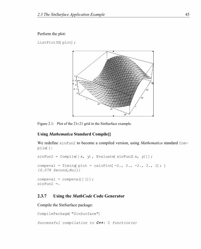
Let Mathematica calculate a plot.
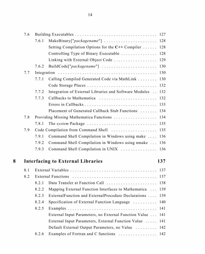
meval = Timing[plot = calcPlot[-2., 2., -2., 2., 1] ][[1]]0.672 Second
2.3 The SinSurface Application Example 45
Perform the plot:
ListPlot3D[plot];
Figure 2.1: Plot of the 21×21 grid in the SinSurface example.
Using Mathematica Standard Compile[]
We redefine sinFun2 to become a compiled version, using Mathematica standard Com-pile[]:
sinFun2 = Compile[{x, y}, Evaluate[sinFun2[x, y]]];
compeval = Timing[plot = calcPlot[-2., 2., -2., 2., 1]; ]{0.078 Second,Null}
compeval = compeval[[1]]; sinFun2 =.
2.3.7 Using the MathCode Code Generator
Compile the SinSurface package:
CompilePackage["SinSurface"]
Successful compilation to C++: 2 function(s)

46 2.3 The SinSurface Application Example
The Generated C++ Code
The generated C++ code from the SinSurface program follows below. Notice that the package name becomes a prefix of the name of the generated C++ function. Thus the Math-ematica function SinSurface‘sinFun2 becomes SinSurface_sinFun2 in C++.
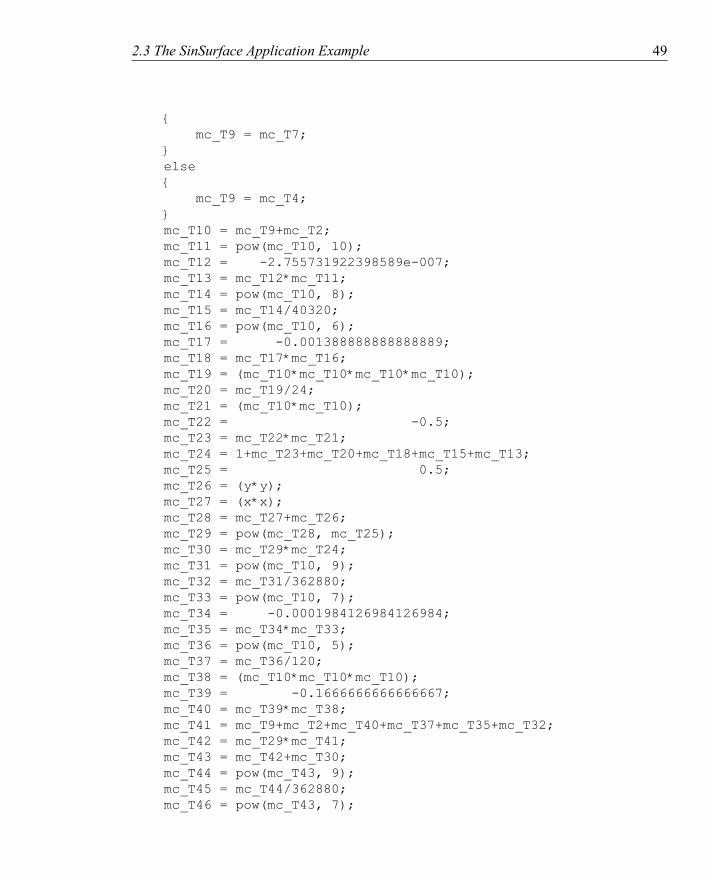
The generated code from SinSurface‘sinFun2 is produced from a large expression by the EvaluateFunctions option. Therefore, common subexpression elimination is performed by the code generator, producing many temporary variables and subexpressions which can be seen in the body of the C++ function SinSurface_sinFun2.
By contrast, the C++ code in the body of function SinSurface_calcPlot produced from the Mathematica function SinSurface‘calcPlot, without being specified by the EvaluateFunctions option, follows the structure of the original code quite closely.
We give a command to type out the text of the generated C++ file:
!!SinSurface.cc
The generated SinSurface.cc file is included below. Note that the exact appearance of this file is very dependent on the exact MathCode version and may differ slightly on your system.#include "SinSurface.h"
#include "SinSurface.icc"
#include <math.h>doubleNN SinSurface_TcalcPlot ( const double &xmin, const double &xmax, const double &ymin, const double &ymax, const int &iter){ int n = 20; double x; double y; int i; int j; int count; count = 1; while (count <= iter) { i = 1; while (i <= n+1) { j = 1; while (j <= n+1) {

2.3 The SinSurface Application Example 47
x = xmin+(((xmax+-xmin)*(i+-1))/n); y = ymin+(((ymax+-ymin)*(j+-1))/n); SinSurface_TxyMatrix(i, j) = SinSurface_TsinFun2 (x, y); j = j+1; } i = i+1; } count = count+1; } return SinSurface_TxyMatrix;}
void SinSurface_TSinSurfaceInit (){; }
double SinSurface_TsinFun2 ( const double &x, const double &y){ int mc_T1; double mc_T2; double mc_T3; double mc_T4; int mc_T5; double mc_T6; double mc_T7; int mc_T8; double mc_T9; double mc_T10; double mc_T11; double mc_T12; double mc_T13; double mc_T14; double mc_T15; double mc_T16; double mc_T17; double mc_T18; double mc_T19; double mc_T20; double mc_T21; double mc_T22; double mc_T23; double mc_T24;

48 2.3 The SinSurface Application Example
double mc_T25; double mc_T26; double mc_T27; double mc_T28; double mc_T29; double mc_T30; double mc_T31; double mc_T32; double mc_T33; double mc_T34; double mc_T35; double mc_T36; double mc_T37; double mc_T38; double mc_T39; double mc_T40; double mc_T41; double mc_T42; double mc_T43; double mc_T44; double mc_T45; double mc_T46; double mc_T47; double mc_T48; double mc_T49; double mc_T50; double mc_T51; double mc_T52; mc_T1 = x < 0; if (mc_T1) { mc_T2 = 3.14159265358979323846; } else { mc_T2 = 0; } mc_T3 = y/x; mc_T4 = atan(mc_T3); mc_T5 = sign (y); mc_T6 = 3.14159265358979323846*mc_T5; mc_T7 = mc_T6/2; mc_T8 = x == 0; if (mc_T8)
2.3 The SinSurface Application Example 49
{ mc_T9 = mc_T7; } else { mc_T9 = mc_T4; } mc_T10 = mc_T9+mc_T2; mc_T11 = pow(mc_T10, 10); mc_T12 = -2.755731922398589e-007; mc_T13 = mc_T12*mc_T11; mc_T14 = pow(mc_T10, 8); mc_T15 = mc_T14/40320; mc_T16 = pow(mc_T10, 6); mc_T17 = -0.001388888888888889; mc_T18 = mc_T17*mc_T16; mc_T19 = (mc_T10*mc_T10*mc_T10*mc_T10); mc_T20 = mc_T19/24; mc_T21 = (mc_T10*mc_T10); mc_T22 = -0.5; mc_T23 = mc_T22*mc_T21; mc_T24 = 1+mc_T23+mc_T20+mc_T18+mc_T15+mc_T13; mc_T25 = 0.5; mc_T26 = (y*y); mc_T27 = (x*x); mc_T28 = mc_T27+mc_T26; mc_T29 = pow(mc_T28, mc_T25); mc_T30 = mc_T29*mc_T24; mc_T31 = pow(mc_T10, 9); mc_T32 = mc_T31/362880; mc_T33 = pow(mc_T10, 7); mc_T34 = -0.0001984126984126984; mc_T35 = mc_T34*mc_T33; mc_T36 = pow(mc_T10, 5); mc_T37 = mc_T36/120; mc_T38 = (mc_T10*mc_T10*mc_T10); mc_T39 = -0.1666666666666667; mc_T40 = mc_T39*mc_T38; mc_T41 = mc_T9+mc_T2+mc_T40+mc_T37+mc_T35+mc_T32; mc_T42 = mc_T29*mc_T41; mc_T43 = mc_T42+mc_T30; mc_T44 = pow(mc_T43, 9); mc_T45 = mc_T44/362880; mc_T46 = pow(mc_T43, 7);

50 2.3 The SinSurface Application Example
mc_T47 = mc_T34*mc_T46; mc_T48 = pow(mc_T43, 5); mc_T49 = mc_T48/120; mc_T50 = (mc_T43*mc_T43*mc_T43); mc_T51 = mc_T39*mc_T50; mc_T52 = mc_T42+mc_T30+mc_T51+mc_T49+mc_T47+mc_T45; return mc_T52;}
doubleNN SinSurface_TxyMatrix(21, 21);
Compiling and Linking the C++ Code
The command MakeBinary compiles the generated C++ code using a C++ compiler (e.g. MicroSoft Visual C++ for Windows platforms or gcc for UNIX or Linux). The object code is by default linked into the executable: SinSurfaceml.exe for calling the compiled code via MathLink.
MakeBinary[];
If any problems are encountered during code compilation, the warning and error messages are shown in the notebook. Otherwise no messages are shown. When MakeBinary is called without arguments, the call applies to the current package.
Installing and Connecting to Mathematica
The command InstallCode installs and connects the external process containing the com-piled and linked SinSurface code.
InstallCode["SinSurface"]
Define an elapsed time-measurement function called AbsTime with a resolution of 1 sec-ond:
SetAttributes[AbsTime,HoldFirst];
AbsTime[x_] := Module[{ start,res }, start = AbsoluteTime[]; res=x; {(AbsoluteTime[]-start) Second,res}];
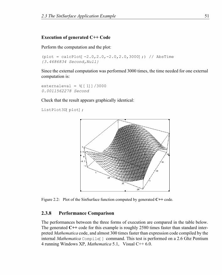
2.3 The SinSurface Application Example 51
Execution of generated C++ Code
Perform the computation and the plot:
(plot = calcPlot[-2.0,2.0,-2.0,2.0,3000];) // AbsTime{3.4686834 Second,Null}
Since the external computation was performed 3000 times, the time needed for one external computation is:
externaleval = %[[1]]/30000.0011562278 Second
Check that the result appears graphically identical:
ListPlot3D[plot];
Figure 2.2: Plot of the SinSurface function computed by generated C++ code.
2.3.8 Performance Comparison
The performances between the three forms of execution are compared in the table below. The generated C++ code for this example is roughly 2580 times faster than standard inter-preted Mathematica code, and almost 300 times faster than expression code compiled by the internal Mathematica Compile[] command. This test is performed on a 2.6 Ghz Pentium 4 running Windows XP, Mathematica 5.1, Visual C++ 6.0.

52 2.3 The SinSurface Application Example
Execution form Time consumed RelativeStandard Mathematica 0.235 203.247.Compile[] 0.063 54.4875External C++ via MathLink 0.0011562278 1.00

2.4 The Gauss Application Example 53
2.4 The Gauss Application ExampleThe Gauss application example uses a textbook Gauss elimination algorithm to solve a lin-ear equation system. Two versions of the Gauss elimination algorithm are presented:
• GaussSolveArrayslice. This algorithm is largely coded using the Matlab-like array slice operations.
• GaussSolveForLoops. This algorithm is coded using traditional for-loops.
Both versions of the algorithm are compiled to C++ code. The performance is measuredboth with and without MathLink overhead.
2.4.1 The Gauss Package
Initialization of the Package
Needs["MathCode`"]
You might want to check which directory you are in and set where you want to be, since some files are generated during the compilation process. You can use the $MCRoot variable that points to the root directory of your MathCode installation.
SetDirectory[$MCRoot<>"/Demos/Gauss"]
Start the Package
BeginPackage["Gauss‘",{MathCodeContexts}];
Define Exported Symbols
Begin["Gauss‘"] GaussSolveArrayslice; GaussSolveForLoops;End[]
Define the Functions and Variables
Begin the “private” implementation section:
Begin["‘Private‘"];

54 2.4 The Gauss Application Example
GaussSolveArrayslice
The GaussSolveArrayslice function
GaussSolveArrayslice[ Real[n_,n_] ain_, Real[n_,m_] bin_ , Integer iterations_]-> Real[n,m] := Module[{ Real[n] dumc, Real[n,n] a, Real[n,m] b, Integer[n] {ipiv, indxr, indxc}, Integer {i,k,l,irow,icol}, Real {pivinv, amax, tmp}, Integer {beficol, afticol, count} }, For[count=1,count<=iterations,count=count+1,( a=ain; b=bin; For [k=1,k<=n, k=k+1, ipiv[[k]]=0 ]; For [i=1,i<=n, i=i+1, (* Algorithm first finds absolutely largest matrix element *) amax=0.0; For [k=1,k<=n, k=k+1, If [ ipiv[[k]]==0 , For [l=1,l<=n, l=l+1, If [ ipiv[[l]]==0 , If [ Abs[a[[k,l]]] > amax, amax= Abs[a[[k,l]]]; irow=k; icol=l ]]]]];
ipiv[[icol]]=ipiv[[icol]]+1; If[ipiv[[icol]]>1, Print["*** Gauss2 input data error ***"]; Break]; If[ irow!=icol , For [k=1,k<=n, k=k+1,

2.4 The Gauss Application Example 55
tmp=a[[irow,k]] ; a[[irow,k]]=a[[icol,k]]; a[[icol,k]]=tmp]; For [k=1,k<=m, k=k+1, tmp=b[[irow,k]] ; b[[irow,k]]=b[[icol,k]]; b[[icol,k]]=tmp] ]; indxr[[i]]=irow; indxc[[i]]=icol; If [ a[[icol,icol]]==0, Print["*** Gauss2 input data error 2 ***"]; Break]; pivinv=1.0 / a[[icol,icol]]; a[[icol,icol]]=1.0;
a[[icol,_]]=a[[icol,_]]*pivinv; b[[icol,_]]=b[[icol,_]]*pivinv; dumc=a[[_,icol]]; For [k=1,k<=n, k=k+1, a[[k,icol]]=0];
a[[icol,icol]]= pivinv;
For [k=1,k<=n, k=k+1, If[ k != icol, a[[k,_]]= a[[k,_]]- dumc[[k]]*a[[icol,_]]; b[[k,_]]= b[[k,_]]- dumc[[k]]*b[[icol,_]] ] ] ];
For [l=n,l>=1, l=l-1, For [k=1,k<=n, k=k+1, tmp= a[[k,indxr[[l]]]]; a[[k,indxr[[l]]]]=a[[k,indxc[[l]]]]; a[[k,indxc[[l]]]]=tmp ]] )]; b];
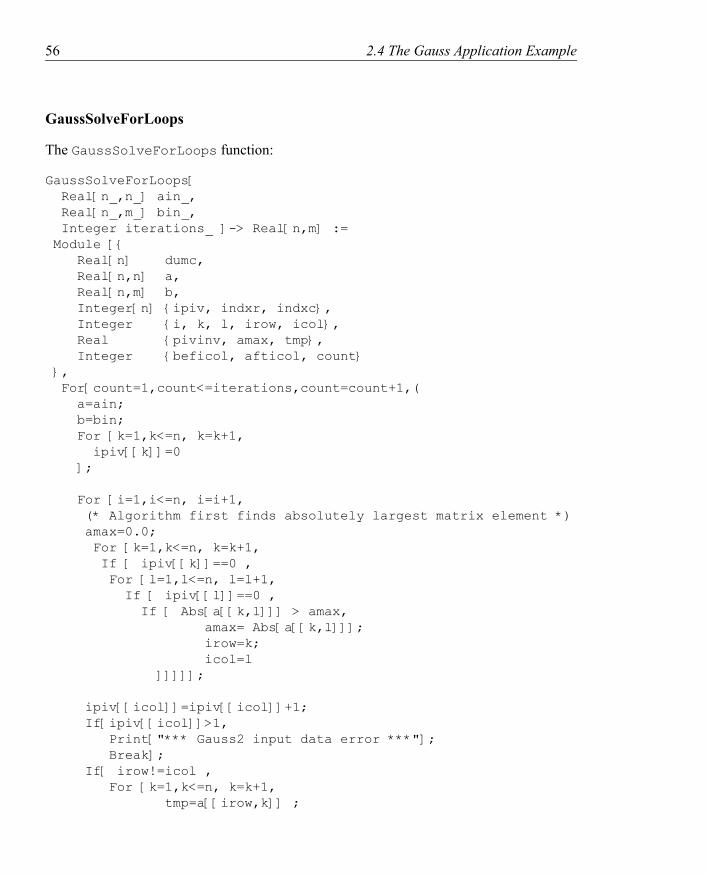
56 2.4 The Gauss Application Example
GaussSolveForLoops
The GaussSolveForLoops function:
GaussSolveForLoops[ Real[n_,n_] ain_, Real[n_,m_] bin_, Integer iterations_ ]-> Real[n,m] := Module [{ Real[n] dumc, Real[n,n] a, Real[n,m] b, Integer[n] {ipiv, indxr, indxc}, Integer {i, k, l, irow, icol}, Real {pivinv, amax, tmp}, Integer {beficol, afticol, count} }, For[count=1,count<=iterations,count=count+1,( a=ain; b=bin; For [k=1,k<=n, k=k+1, ipiv[[k]]=0 ]; For [i=1,i<=n, i=i+1, (* Algorithm first finds absolutely largest matrix element *) amax=0.0; For [k=1,k<=n, k=k+1, If [ ipiv[[k]]==0 , For [l=1,l<=n, l=l+1, If [ ipiv[[l]]==0 , If [ Abs[a[[k,l]]] > amax, amax= Abs[a[[k,l]]]; irow=k; icol=l ]]]]];
ipiv[[icol]]=ipiv[[icol]]+1; If[ipiv[[icol]]>1, Print["*** Gauss2 input data error ***"]; Break]; If[ irow!=icol , For [k=1,k<=n, k=k+1, tmp=a[[irow,k]] ;

2.4 The Gauss Application Example 57
a[[irow,k]]=a[[icol,k]]; a[[icol,k]]=tmp]; For [k=1,k<=m, k=k+1, tmp=b[[irow,k]] ; b[[irow,k]]=b[[icol,k]]; b[[icol,k]]=tmp] ]; indxr[[i]]=irow; indxc[[i]]=icol; If [ a[[icol,icol]]==0, Print["*** Gauss2 input data error 2 ***"]; Break]; pivinv=1.0 / a[[icol,icol]]; a[[icol,icol]]=1.0;
For [k=1,k<=n, k=k+1, a[[icol,k]]=a[[icol,k]]*pivinv]; For [k=1,k<=m, k=k+1, b[[icol,k]]=b[[icol,k]]*pivinv]; For [k=1,k<=n, k=k+1, dumc[[k]]=a[[k,icol]];a[[k,icol]]=0];
a[[icol,icol]]= pivinv;
For [k=1,k<=n, k=k+1, If [ k != icol, For [l=1,l<=n, l=l+1, a[[k,l]]= a[[k,l]]- dumc[[k]]* a[[icol,l]]]; For [l=1,l<=m, l=l+1, b[[k,l]]= b[[k,l]]- dumc[[k]]* b[[icol,l]]] ]] ];
For [l=n,l>=1, l=l-1, For [k=1,k<=n, k=k+1, tmp= a[[k,indxr[[l]]]]; a[[k,indxr[[l]]]]=a[[k,indxc[[l]]]]; a[[k,indxc[[l]]]]=tmp ]] )]; b];

58 2.4 The Gauss Application Example
The Compiled GaussSolveForLoops function, using Compile[] GaussSolveForLoopsC=Compile[{{ain,_Real,2},{bin,_Real,2},{iterations,_Integer}},Module[{n=Dimensions[ain][[1]],m=Dimensions[bin][[2]],dumc=Table[0.0,{n}],a=Table[0.0,{n},{n}],b=Table[0.0,{n},{m}],ipiv=Table[0,{n}], indxr=Table[0,{n}], indxc=Table[0,{n}], i=0, k=0, l=0, irow=0, icol=0, pivinv=0.0, amax=0.0, tmp=0.0, beficol=0, afticol=0, count=0 },For[count=1,count<=iterations,count=count+1,( a=ain; (* The arguments are always generated as const references and therefore cannot be changed.Actuall we get waste of space and time here when they are copied. *) b=bin; For [k=1,k<=n, k=k+1,ipiv[[k]]=0]; For [i=1,i<=n, i=i+1, (* Algorithm first finds absolutely largest matrix element *) amax=0.0; For [k=1,k<=n, k=k+1, If [ ipiv[[k]]==0 , For [l=1,l<=n, l=l+1, If [ ipiv[[l]]==0 , If [ Abs[a[[k,l]]] > amax, amax= Abs[a[[k,l]]];
irow=k; icol=l ]]]]];
ipiv[[icol]]=ipiv[[icol]]+1; If[ipiv[[icol]]>1, Print["*** Gauss2 input data error ***"]; Break]; If[ irow!=icol ,

2.4 The Gauss Application Example 59
For [k=1,k<=n, k=k+1, tmp=a[[irow,k]] ; a[[irow,k]]=a[[icol,k]]; a[[icol,k]]=tmp]; For [k=1,k<=m, k=k+1, tmp=b[[irow,k]] ; b[[irow,k]]=b[[icol,k]]; b[[icol,k]]=tmp] ]; indxr[[i]]=irow; indxc[[i]]=icol; If [ a[[icol,icol]]==0, Print["*** Gauss2 input data error 2 ***"]; Break]; pivinv=1.0 / a[[icol,icol]]; a[[icol,icol]]=1.0; For [k=1,k<=n, k=k+1, a[[icol,k]]=a[[icol,k]]*pivinv]; For [k=1,k<=m, k=k+1, b[[icol,k]]=b[[icol,k]]*pivinv]; For [k=1,k<=n, k=k+1, dumc[[k]]=a[[k,icol]];a[[k,icol]]=0]; a[[icol,icol]]= pivinv;
For [k=1,k<=n, k=k+1, If [ k != icol, For [l=1,l<=n, l=l+1, a[[k,l]]= a[[k,l]]- dumc[[k]]* a[[icol,l]]];
For [l=1,l<=m, l=l+1, b[[k,l]]= b[[k,l]]- dumc[[k]]* b[[icol,l]]] ]] ];For [l=n,l>=1, l=l-1, For [k=1,k<=n, k=k+1, tmp= a[[k,indxr[[l]]]]; a[[k,indxr[[l]]]]=a[[k,indxc[[l]]]]; a[[k,indxc[[l]]]]=tmp ]])]; b]];

60 2.4 The Gauss Application Example
End of the Gauss Package
End of the package:
End[];EndPackage[];
2.4.2 Executing the Interpreted Version in Mathematica
First we need to create two arrays to be used as input for the solver.
a=Table[Random[],{10},{10}];b=Table[Random[],{10},{2}];
Run GaussSolveArrayslice
The loop time may be too short for reliable measurements. It is only 3- 4 seconds combined with a resolution of 1 second. The relevant factor for a 1.5 GHz computer is 10.
factor=10; loops=1*factor;
Call the solver:s=(c=GaussSolveArrayslice[a,b,loops];)//Timing;meval=s[[1]];Print["TIMING FOR NON-COMPILED VERSION=",meval];
TIMING FOR NON-COMPILED VERSION= 0.1734 Second
Run the For-loop Version
Execute the version with for-loops:
s=(c=GaussSolveForLoops[a,b,loops];)//Timing;mevalFor=s[[1]];Print["TIMING FOR NON-COMPILED VERSION (FOR-LOOPS)=",mevalFor];
TIMING FOR NON-COMPILED VERSION (FOR-LOOPS)= 0.1078 Second
2.4.3 Generation of C++ code
The command CompilePackage translates the package to C++ code:

2.4 The Gauss Application Example 61
CompilePackage["Gauss"]Successful compilation to C++: 2 function(s)
The Produced C++ Code for Gauss
To save space, we only show the C++ code of the translated GaussSolveArrayslicefunction (which in fact also contains a few for-loops). The actual code generated on your system may differ slightly, as it is very dependent on the exact version of MathCode used.#include "Gauss.h"#include "Gauss.icc"#include <math.h>
void Gauss_TGaussInit (){;}
doubleNN Gauss_TGaussSolveArraySlice ( const doubleNN &ain, const doubleNN &bin , const int &iterations){ int n = ain.dimension(1); int m = bin.dimension(2); doubleN dumc(n); doubleNN a(n, n); doubleNN b(n, m); intN ipiv(n); intN indxr(n); intN indxc(n); int i; int k; int l; int irow; int icol; double pivinv; double amax; double tmp; int beficol; int afticol; int count; count = 1; while (count <= iterations) { a = ain; b = bin; k = 1;
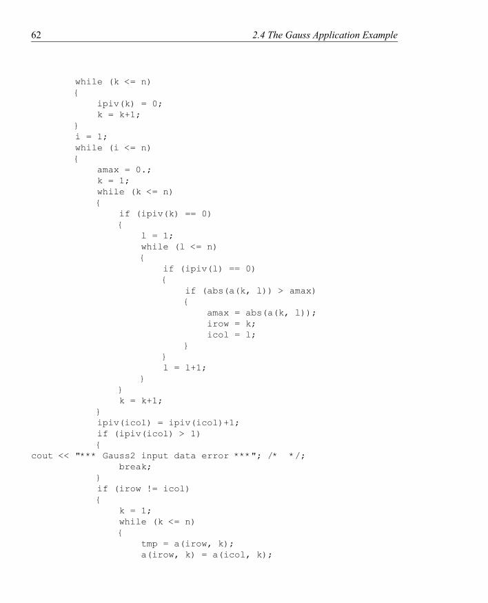
62 2.4 The Gauss Application Example
while (k <= n) { ipiv(k) = 0; k = k+1; } i = 1; while (i <= n) { amax = 0.; k = 1; while (k <= n) { if (ipiv(k) == 0) { l = 1; while (l <= n) { if (ipiv(l) == 0) { if (abs(a(k, l)) > amax) { amax = abs(a(k, l)); irow = k; icol = l; } } l = l+1; } } k = k+1; } ipiv(icol) = ipiv(icol)+1; if (ipiv(icol) > 1) {cout << "*** Gauss2 input data error ***"; /* */; break; } if (irow != icol) { k = 1; while (k <= n) { tmp = a(irow, k); a(irow, k) = a(icol, k);

2.4 The Gauss Application Example 63
a(icol, k) = tmp; k = k+1; } k = 1; while (k <= m) { tmp = b(irow, k); b(irow, k) = b(icol, k); b(icol, k) = tmp; k = k+1; } } indxr(i) = irow; indxc(i) = icol; if (a(icol, icol) == 0) { cout << "*** Gauss2 input data error 2 ***"; cout << "\n"; break; } pivinv = 1./a(icol, icol); a(icol, icol) = 1.; a.Set(icol, All,a(icol, All)*pivinv); b.Set(icol, All,b(icol, All)*pivinv); dumc = a(All, icol); k = 1; while (k <= n) { a(k, icol) = 0; k = k+1; } a(icol, icol) = pivinv; k = 1; while (k <= n) { if (k != icol) { a.Set(k, All,a(k, All)+-(dumc(k)*a(icol, All))); b.Set(k, All,b(k, All)+-(dumc(k)*b(icol, All))); } k = k+1; }
64 2.4 The Gauss Application Example
i = i+1; } l = n; while (l >= 1) { k = 1; while (k <= n) { tmp = a(k, indxr(l)); a(k, indxr(l)) = a(k, indxc(l)); a(k, indxc(l)) = tmp; k = k+1; } l = l+-1; } count = count+1; } return b;}doubleNN Gauss_TGaussSolveForLoops ( const doubleNN &ain, const doubleNN &bin, const int &iterations){ int n = ain.dimension(1); int m = bin.dimension(2); doubleN dumc(n); doubleNN a(n, n); doubleNN b(n, m); intN ipiv(n); intN indxr(n); intN indxc(n); int i; int k; int l; int irow; int icol; double pivinv; double amax; double tmp; int beficol; int afticol; int count; count = 1; while (count <= iterations)
2.4 The Gauss Application Example 65
{ a = ain; b = bin; k = 1; while (k <= n) { ipiv(k) = 0; k = k+1; } i = 1; while (i <= n) { amax = 0.; k = 1; while (k <= n) { if (ipiv(k) == 0) { l = 1; while (l <= n) { if (ipiv(l) == 0) { if (abs(a(k, l)) > amax) { amax = abs(a(k, l)); irow = k; icol = l; } } l = l+1; } } k = k+1; } ipiv(icol) = ipiv(icol)+1; if (ipiv(icol) > 1) {cout << "*** Gauss2 input data error ***"; /* */; break; } if (irow != icol) { k = 1;

66 2.4 The Gauss Application Example
while (k <= n) { tmp = a(irow, k); a(irow, k) = a(icol, k); a(icol, k) = tmp; k = k+1; } k = 1; while (k <= m) { tmp = b(irow, k); b(irow, k) = b(icol, k); b(icol, k) = tmp; k = k+1; } } indxr(i) = irow; indxc(i) = icol; if (a(icol, icol) == 0) { cout << "*** Gauss2 input data error 2 ***"; cout << "\n"; break; } pivinv = 1./a(icol, icol); a(icol, icol) = 1.; k = 1; while (k <= n) { a(icol, k) = a(icol, k)*pivinv; k = k+1; } k = 1; while (k <= m) { b(icol, k) = b(icol, k)*pivinv; k = k+1; } k = 1; while (k <= n) { dumc(k) = a(k, icol); a(k, icol) = 0; k = k+1;

2.4 The Gauss Application Example 67
} a(icol, icol) = pivinv; k = 1; while (k <= n) { if (k != icol) { l = 1; while (l <= n) { a(k, l) = a(k, l)+-(dumc(k)*a(icol, l)); l = l+1; } l = 1; while (l <= m) { b(k, l) = b(k, l)+-(dumc(k)*b(icol, l)); l = l+1; } } k = k+1; } i = i+1; } l = n; while (l >= 1) { k = 1; while (k <= n) { tmp = a(k, indxr(l)); a(k, indxr(l)) = a(k, indxc(l)); a(k, indxc(l)) = tmp; k = k+1; } l = l+-1; } count = count+1; } return b;}

68 2.4 The Gauss Application Example
2.4.4 Building the Executable
Call MakeBinary to compile the generated C++ code and build the executable(s).
MakeBinary[]
Here, no package is given to MakeBinary. This means that the current package should be used.
2.4.5 Installing Compiled Code
Interpreted versions are removed, and compiled ones are used instead by using the In-stallCode function:
InstallCode["Gauss"];
2.4.6 Prepare for Execution
Define a time measurement function, AbsTime:
SetAttributes[AbsTime,HoldFirst];AbsTime[x_] := Module[{start,res},
start = AbsoluteTime[];res=x;{(AbsoluteTime[]-start) Second,res}
];
2.4.7 External Execution
External Execution of Array Slice Version
Call the version of GaussSolve which contains array slice operations. Repeat the solution process several thousand times in order to get a measurable time. The external compiled GaussSolveArrayslice function is called via MathLink, in the same way an internal Mathematica function is called. Recall that we defined test matrices a and b earlier. The same matrices will be used for this test.
loops=8000 * factor;externaleval=((cc=GaussSolveArrayslice[a,b,loops]; ) //AbsTime)[[1]]/loops0.000253510758 Second

2.4 The Gauss Application Example 69
External Array Slice Version, MathLink in each Iteration
Call the GaussSolve externally-compiled code via MathLink as before, but perform the so-lution process only once per call. This causes the MathLink communication overhead to dominate (almost by a factor of 80) over the time needed to perform the actual solution pro-cess.
loops=100*factor;externalevalPass=((Do[cc=GaussSolveArrayslice[aa,bb,1],{loops}];) //AbsTime)[[1]]/loops0.000013124328 Second
External Execution of For-Loop Version
The for-loop version of GaussSolve is executed externally several thousand times, which is sufficient to get an execution time long enough for reliable measurements. The compiled code is slightly faster than the array slice version, since the generated code avoids some overhead in creating array objects. On the other hand, the array slice code is almost as fastand is more concise and convenient to write and understand.
loops=8000* factor;externalevalFor=((cc=GaussSolveForLoops[aa,bb,loops]; ) //AbsTime)[[1]]/loops0.000013437156 Second
External For-loop Version, MathLink in each Iteration
As before with the array slice version, if a call via MathLink is performed in each iteration, the MathLink communication overhead will dominate over the actual computation time.
loops=100;externalevalPassFor= ((Do[cc=GaussSolveForLoops[aa,bb,1],{loops}];) //AbsTime)[[1]]/loops0.0012497360 Second
External Array Slice Version with InlineFlag and No Range
If setting InlineFlag->True in the compilation options, certain array access functions and array slice operators will be inlined in the generated code. Setting InlineFlag->Truealso changes the default value of RangeCheckFlag to False so no range checking is per-formed in the generated code. These flags are described in section 7.3.2 on page 119.
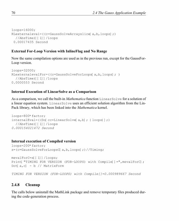
70 2.4 The Gauss Application Example
loops=16000;RLexternaleval=((c=GaussSolveArrayslice[a,b,loops];) //AbsTime)[[1]]/loops 0.00017435 Second
External For-Loop Version with InlineFlag and No Range
Now the same compilation options are used as in the previous run, except for the GaussFor-Loop version.
loops=32000;RLexternalevalFor=((c=GaussSolveForLoops[a,b,loops]; ) //AbsTime)[[1]]/loops0.0000553 Second
Internal Execution of LinearSolve as a Comparison
As a comparison, we call the built-in Mathematica function LinearSolve for a solution of a linear equation system. LinearSolve uses an efficient solution algorithm from the Lin-Pack library, which has been linked into the Mathematica kernel.
loops=800*factor;internalEval=((Do[cc=LinearSolve[a,b]; {loops}];) //AbsTime)[[1]]/loops0.000154021472 Second
Internal execution of Compiled versionloops=200*factor;s=(c=GaussSolveForLoopsC[a,b,loops];)//Timing;
mevalForC=s[[1]]/loops;Print["TIMING FOR VERSION (FOR-LOOPS) with Compile[]=",mevalForC];Dot[a,c] - b // MatrixForm
TIMING FOR VERSION (FOR-LOOPS) with Compile[]=0.000989667 Second
2.4.8 Cleanup
The calls below uninstall the MathLink package and remove temporary files produced dur-ing the code-generation process.

2.4 The Gauss Application Example 71
UninstallCode["Gauss"]CleanMathCodeFiles[]
CleanMathCodeFiles can also be given an argument to specify which package to cleanup. The default is to clean up the last package compiled, which is used above.

72 2.4 The Gauss Application Example

3.1 Examples of Array Operations 73
Chapter 3 Matrix and Vector Operations
In many engineering applications, matrices and matrix manipulation operations are very common. The availability of an easy-to-use and short-handed notation for manipulating ma-trices is important for these application domains. Thus, we have extended the Part ([[ ]]) operation in Mathematica to fulfill this objective.
The basic set of matrix operations in typed Mathematica presented in this chapter is currently limited to operations on array sections. Declaration of array variables is described in Chapter 5 and dynamic array allocation and initialization in Chapter 6.
The syntax is inspired by the syntax used by Matlab, Fortran90 and Modelica. This syntax is supported by the MathCode code generator for up to 4-dimensional arrays and within Mathematica for an arbitrary number of dimensions.
Only operations on homogenous arrays, i.e. where all elements have the same type, are supported by the code generator. Also, arrays must have a matrix-like shape, i.e. there must be the same number of elements in each row or column of a matrix. This constraint applies to generated code, but not necessarily within Mathematica.
3.1 Examples of Array OperationsBefore going into detail about the index notation, the differences between vectors and ma-trices, and operations on those, we show below a few array-slice operations to give you an intuitive understanding of the process. First create a small matrix A with symbolic compo-nents of the form a[i,j]:
A=Table[a[i,j], {i,4},{j,5}]
Result:
{{a[1,1], a[1,2], a[1,3], a[1,4], a[1,5]}, {a[2,1], a[2,2], a[2,3], a[2,4], a[2,5]}, {a[3,1], a[3,2], a[3,3], a[3,4], a[3,5]}, {a[4,1], a[4,2], a[4,3], a[4,4], a[4,5]}}

74 3.2 Index Range Notation
Extract row 2 and 3:
A[[2|3,_]]
{{a[2,1], a[2,2], a[2,3], a[2,4], a[2,5]}, {a[3,1], a[3,2], a[3,3], a[3,4], a[3,5]}}
Extract all but the first two columns, i.e. from the 3rd to the last column:
A[[_, 3|_]]
{{a[1,3], a[1,4], a[1,5]}, {a[2,3], a[2,4], a[2,5]}, {a[3,3], a[3,4], a[3,5]}, {a[4,3], a[4,4], a[4,5]}}
3.2 Index Range NotationWhen manipulating sections of arrays, it is important to have a concise and readable notation for index ranges. Such a notation is currently missing from standard Mathematica. There is a standard colon (:) notation used both by Matlab and Fortran90, which unfortunately was not possible to employ directly in Mathematica due to parsing problems. Instead we chose the vertical bar (|) which has a graphical layout similar to that of a colon and parses without problems in Mathematica. For example, an index range from 2 to n is expressed as follows in Matlab and Fortran90:
2:n
and in our Mathematica notation as:
2|n
3.2.1 Omitting End of Index Range
There are index-range colon expressions in Matlab and Fortran90 without a right-hand side, which implies that the largest value implied by the context should be used. For example:
2:

3.2 Index Range Notation 75
The 2: in Matlab or Fortran90 means the same as 2:n if there are at most n elements in the matrix dimension where this range is used, since n is then the largest value implied by con-text.
In Mathematica the vertical bar is always a binary operator, which means that a placeholder must be provided for the missing right-hand side. We use underscore (_) as this placeholder, since that notation is already used for placeholders in Mathematica patterns. Thus the Matlab and Fortran90 example 2: is represented by the following Mathematicasyntax:
2|_
3.2.2 Omitting Start of Index Range
Alternatively, the left-hand side of the colon can be omitted in Matlab and Fortran90, for example:
:n-1
This means that the lowest index value should be used, which is always 1 in Matlab and Fortran90, as well as in Mathematica. The Mathematica counterpart then becomes:
1|n-1
3.2.3 Omitting Both Start and End of a Range
It is possible to omit both the start and the end of an index range, which in Matlab and Fortran90 becomes a single colon and is equivalent to 1:n for a dimension of size n:
:
In Mathematica this can be represented by:
1|_
This is a very common special case denoting the whole range of a matrix dimension. There-fore we also provide the compact notation of a single underscore (_) to represent the whole range of a dimension:
_
76 3.3 Vectors Versus Rows and Columns
3.3 Vectors Versus Rows and ColumnsIn Matlab all arrays including rows or columns of matrices are 2-dimensional matrices, whereas in Mathematica and Fortran90 either 1-dimensional vectors or 2-dimensional row vectors or column vectors are possible.
3.3.1 One-dimensional Vectors
One-dimensional vector variables are type declared using one index dimension, e.g.:
Declare[ Real[5] x;]
A one-dimensional vector (i.e. a 1×5 array value with symbolic components might appear as follows in Mathematica:
{x[1], x[2], x[3], x[4], x[5]}
3.3.2 Row Vectors
A row vector extracted from a matrix is always a two-dimensional (e.g. 1×n) array in Mat-lab, whereas in Mathematica and Fortran90 it can be either a two-dimensional or a one-di-mensional entity. Most operations in Mathematica and Fortran90 accept either representa-tion by performing automatic type conversion to the appropriate vector type, but certain op-erations such as dot product can be sensitive to the type of vector. An extracted Mathematicarow-vector with symbolic components can appear as follows:
{ {a[2,1], a[2,2], a[2,3], a[2,4], a[2,5]} }
or with numeric components:
{ {1.1, 3.5, 2.3, 5., 6.2} }
The corresponding type is:
Real[1,5]
Thus, a more appropriate term for row vector would be row matrix, since it really is a matrix.
3.3.3 Column Vectors
Analogous to the case for row vectors, a column vector extracted from a matrix is always a
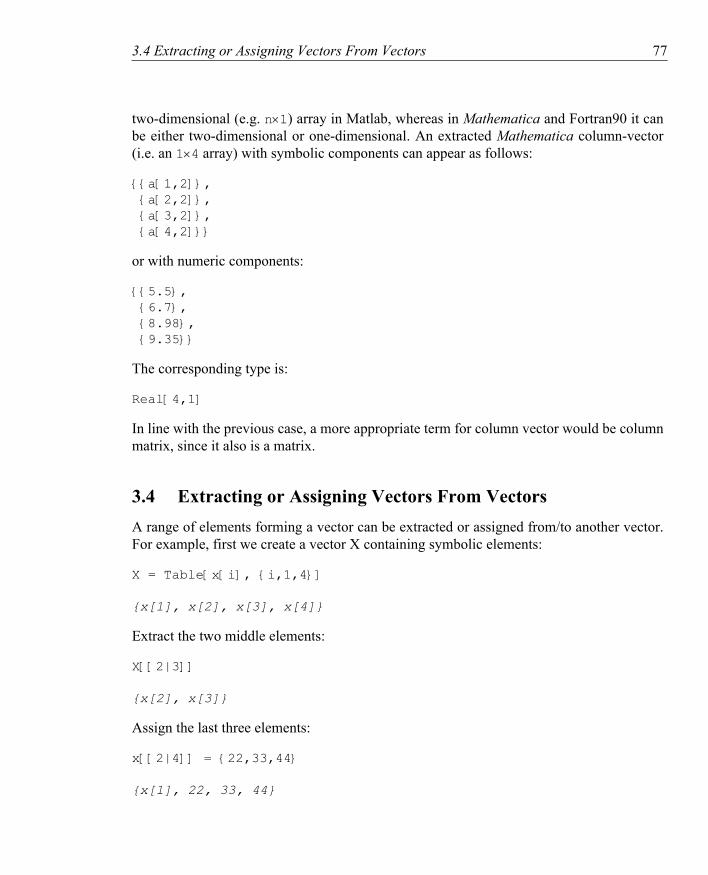
3.4 Extracting or Assigning Vectors From Vectors 77
two-dimensional (e.g. n×1) array in Matlab, whereas in Mathematica and Fortran90 it can be either two-dimensional or one-dimensional. An extracted Mathematica column-vector (i.e. an 1×4 array) with symbolic components can appear as follows:
{{a[1,2]}, {a[2,2]}, {a[3,2]}, {a[4,2]}}
or with numeric components:
{{5.5}, {6.7}, {8.98}, {9.35}}
The corresponding type is:
Real[4,1]
In line with the previous case, a more appropriate term for column vector would be column matrix, since it also is a matrix.
3.4 Extracting or Assigning Vectors From VectorsA range of elements forming a vector can be extracted or assigned from/to another vector. For example, first we create a vector X containing symbolic elements:
X = Table[x[i], {i,1,4}]
{x[1], x[2], x[3], x[4]}
Extract the two middle elements:
X[[2|3]]
{x[2], x[3]}
Assign the last three elements:
x[[2|4]] = {22,33,44}
{x[1], 22, 33, 44}

78 3.5 Extracting Vectors From Matrices
3.5 Extracting Vectors From MatricesEither one-dimensional vectors or two-dimensional row- or column vectors can be extracted from rows and columns of matrices. However, in almost all cases the one-dimensional ver-sion is desired when programming in Mathematica or Fortran90. This results in slightly more efficient code and allows for indexing the vector using one index instead of two.
3.5.1 Extracting One-dimensional Vectors
Extraction operators using a single number or expression, e.g. 2 below, will always produce 1-dimensional vectors. For example:
Extraction of a row as a 1-dimensional vector:
A[[2,_]]
{a[2,1],a[2,2],a[2,3],a[2,4],a[2,5]}
Extraction of a column as a 1-dimensional vector:
A[[_,2]]
{a[1,2],a[2,2],a[3,2],a[4,2]}
3.5.2 Extracting Vectors as Submatrices of Shape 1×n or n×1The index-range notations {i2} and i1|i2 always produce vectors as two-dimensional submatrices, whereas just i2 results in one-dimensional vectors as presented in Section 3.5.1. For example:
Extraction of a column as a column-vector, i.e. as an n×1 submatrix:
A[[_,{2}]]
{{a[1,2]}, {a[2,2]}, {a[3,2]}, {a[4,2]}}
The n1|n2 syntax always gives a submatrix. Here it is used to extract a column-vector which is an n x 1 submatrix as in the previous example:
A[[_,4|4]]

3.6 Assigning Vectors to Rows or Columns of Matrices 79
{{a[1,4]}, {a[2,4]}, {a[3,4]}, {a[4,4]}}
Extraction of a row as a 1xn submatrix:
A[[{2},_]]
{ {a[2,1],a[2,2],a[2,3],a[2,4],a[2,5]} }
The notation {2} is equivalent to 2|2.
3.6 Assigning Vectors to Rows or Columns of Matrices
The examples in this section assume that A is re-initialized as shown in section 3.1 before execution of each example.
The following sets the contents of a row to the contents of a vector. For example, setting row 2 to another value:
A[[2,_]] = {11, 22, 33, 44, 55}
{{a[1,1], a[1,2], a[1,3], a[1,4], a[1,5]}, {11, 22, 33, 44, 55 }, {a[3,1], a[3,2], a[3,3], a[3,4], a[3,5]}, {a[4,1], a[4,2], a[4,3], a[4,4], a[4,5]}}
Due to the list representation of arrays in Mathematica, it is possible to get identical results by only giving a row dimension, e.g.:
A[[2]] = {11, 22, 33, 44, 55}
A column can be assigned the value of a one-dimensional vector:
A[[_,3]] = {11, 22, 33, 44}
Result:
{{a[1,1], a[1,2], 11, a[1,4], a[1,5]}, {a[2,1], a[2,2], 22, a[2,4], a[2,5]}, {a[3,1], a[3,2], 33, a[3,4], a[3,5]}, {a[4,1], a[4,2], 44, a[4,4], a[4,5]}}

80 3.7 Extracting and Assigning Arbitrary Submatrices
Row- and column vectors or two-dimensional shapes 1×n or n×1 can also be assigned to rows or columns of a matrix. However, be sure to also specify such shapes on the left-hand side. For example, assigning a 1×n row vector:
A[[_,2|2]] = {{11, 22, 33, 44, 55}}
Assigning an n×1 column vector:
A[[_,3|3]] = {{11}, {22}, {33}, {44}}
3.7 Extracting and Assigning Arbitrary SubmatricesArbitrary submatrices can be extracted or assigned by using complete range specifications. For example:
Extracting a 2 × 2 submatrix from A:
A[[2|3, 2|3]]
Result:
{{a[2,2], a[2,3]}, {a[3,2], a[3,3]}}
Assigning values to a submatrix of A:
A[[2|3, 2|3]] = {{1, 2}, {3, 4}};
Result:
A // MatrixForm1
{ {a[1,1], a[1,2], a[1,3], a[1,4], a[1,5]}, {a[2,1], 1, 2, a[2,4], a[2,5]}, {a[3,1], 3, 4, a[3,4], a[3,5]}, {a[4,1], a[4,2], a[4,3], a[4,4], a[4,5]} }
1. Actually, a matrix formatted using MatrixForm in a real notebook looks nicer than what is shown in this text.

3.8 Promotion of Scalars to Vectors or Matrices 81
3.8 Promotion of Scalars to Vectors or MatricesThe standard Mathematica assignment operation will allow the assigning of a scalar value to a matrix variable even though it has been declared and initialized as a matrix:
A = 5
A has now been converted to a scalar integer variable with the value 5:
A
5
Such assignments will give rise to a type error in generated C++ code. However, it is possi-ble to perform elementwise initialization of arrays by scalar values both in Mathematica and in generated code by specifying the dimensions in the left-hand side. Then the scalar value will automatically be promoted to constant array of compatible shape when performing the assignment.
For example, the two last columns (from 4 to the end) of A should be set to zero. The scalar 0 in the example below can be regarded as being promoted to a 4×2 constant array of zeroes before performing the actual assignment.
A[[_, 4|_]] = 0;
A // MatrixForm
{{a[1, 1], a[1, 2], a[1, 3], 0, 0 }, {a[2, 1], 1 , 2 , 0, 0 }, {a[3, 1], 3 , 4 , 0, 0 }, {a[4, 1], a[4, 2], a[4, 3], 0, 0 }}
It is possible to set all elements of the array to the same scalar value:
A[[_,_]] = 555;
A // MatrixForm
{{555, 555, 555, 555, 555 }, {555, 555, 555, 555, 555 }, {555, 555, 555, 555, 555 }, {555, 555, 555, 555, 555 }}

82 3.9 An Example Matrix Function
3.9 An Example Matrix FunctionThis example function, called matrixtestfunc, is completely meaningless from a com-putational point of view, but still illustrates how matrices can be declared as formal param-eters and local arrays, returned as function values, and operated on by a number of assign-ment and value-extraction array section operations. The local variables a, b, c and d are sim-ply initialized to integer constants. The syntax used for declaring arrays is explained in more detail in Chapter 5.
matrixtestfunc[Real[n_,n_] ain_]->Real[n,n] := Module[{ Real[n,n] y; Integer {a=2,b=3,c=2,d=4}; }, y[[_,2]]=ain[[_,2]]; y[[_,a|_]]=ain[[_,a|_]]; y[[_,c|d]]=ain[[_,c|d]]; y[[a,_]]=ain[[a,_]]; y[[a|_,_]]=ain[[a|_,_]]; y[[a|b,_]]=ain[[a|b,_]]; y[[a|_,c|_]]=ain[[a|_,c|_]]; y[[a|_,c|d]]=ain[[a|_,c|d]]; y[[a|b,c|_]]=ain[[a|b,c|_]]; y[[a|b,c|d]]=ain[[a|b,c|d]]; y[[_,b]]=ain[[_,b]]; y[[a,_]]=ain[[a,_]]; y];
3.10 Current LimitationsThe current MathCode code generator is limited to array section operations on up to 4-di-mensional homogenous arrays. Also, it is currently not possible to specify a different stride (i.e. step size) than the default 1, as can be done in both Matlab and Fortran90.

4.1 Why Type Declarations? 83
Chapter 4 Rationale for Type Declarations in Mathematica
Previously, in Chapter 1, we presented some examples of static type declarations in Mathe-matica code needed to use the MathCode code generator. In this chapter, the type declara-tion notation, or “type system”, is motivated and presented in broader perspective—a type system can be used for more purposes than just to provide the necessary typing needed for a code generator.
The main reason to introduce static typing in Mathematica is to be able to generate efficient code in languages such as C++ and Fortran90.
The static type system presented here is designed to be well integrated into Mathematica. The syntax is Mathematica compatible, which makes it possible to use the type extensions in ordinary Mathematica code.
The type declarations are treated as code annotations within Mathematica, i.e. loosely associated additional information. Thus, they have no effect on execution and symbolic transformations within Mathematica apart from introducing the names of declared types and variables in the current Mathematica context. The only exceptions are typed array variable declarations with or without initialization parts, where the declared variable is allocated automatically to the specified dimensions and size.
Certain advanced features of the type system such as class declarations, records, etc.,which sometimes are briefly hinted at in the text, are not implemented in the current version of MathCode, but are planned to become available in a future version.
4.1 Why Type Declarations?There are several reasons why a static type system is a useful extension to Mathematica:
• Precise static type information is needed for generation of efficient executable code.• A type checker is useful for finding errors during software development in Mathematica.• Object-oriented typing is useful to handle complexity when building large applications
84 4.2 Types for Code Generation
and equation-based simulation models.
Additional requirements of a type system are:
• Ease of use. The type system should be easy to understand and use.• Readability and standardization. The type notation should be readable and conform to
common program language standards, as well as to relevant Mathematica conventions.• Compatibility. Typed Mathematica code should be able to be executed together with
untyped code. Adding type information should be a pure extension—existing code should, for the most part, not need to be changed.
We discuss below the motivation behind a static type system in more detail.
4.2 Types for Code GenerationPrecise static type information is needed for translating Mathematica into efficient code in strongly typed languages such as C++, Fortran90 and Java. It is also needed for more effi-cient internal compilation of Mathematica to efficient code as evidenced by the type infor-mation parameters to the standard Mathematica Compile function.
Experience from research on code generation to C++ and Fortran90 from the ObjectMath1 extension to Mathematica made it clear that precise static type information could not always be automatically deduced from dynamically typed Mathematica code,especially when list structures (arrays) were involved. Therefore explicit declaration of static type information was introduced. However, in many cases it is possible to automatically derive static type information through type inference.
Precise static typing is especially important to provide consistent handling of arraysbetween Mathematica, C++, Fortran90, Java, etc., including compatibility with array representations used in common numerical subroutine libraries.
4.3 The Need for Type Checking Debugging Mathematica programs can be hard. Simple spelling errors and other mistakes may cause pattern matching to fail, which causes huge unevaluated expressions to be re-turned to the user. It is usually not so easy to realize where the source of the error is located. Partial dynamic type checking of function parameters can be turned on, but will only be able to catch errors for the particular test cases which are used during debugging and testing.
A static type checker can be of great help in finding simple mistakes such as spelling
1. Article in IEEE Software, July 1995.
4.4 Types for Object Oriented Simulation Modeling 85
errors of variables or function names, wrong number of arguments to functions, mismatch of actual argument types and formal parameter types, etc. Concerning parameter types, most built-in Mathematica functions have numeric parameters which will be assigned the type Real in the static type system. The static type Real is, of course, an approximation, since there are several numeric forms in Mathematica such as infinite precision numbers and fractions. However, the approximation to Real fits well with code generation to staticallytyped languages such as C++ or Fortran90 as well as being a reasonable static type approximation for execution within Mathematica, since the exact numeric type may change dynamically during execution.
A relevant question is whether the static type system would be able to detect enough errors, since most functions in Mathematica are numeric anyway, and declaring the type Real for function parameters and results will not add considerable information. There are however many functions which accept parameters that are vectors and arrays of different forms and for which precise type information is quite useful for type checking. Other functions accept parameters which are records represented as tagged tuples. Additionally, checking the number of function parameters and whether a function or variable has been declared would catch many common mistakes by Mathematica programmers.
4.4 Types for Object Oriented Simulation ModelingSimulation models are usually constructed to simulate a model of aspects of the external world. This is precisely where object orientation is most useful. For example, typical me-chanical systems consist of a number of mechanical components which can be described by classes containing equations that describe motion, forces, material properties, etc. Simula-tion models of mechanical and other systems can be put together by connecting such objects from class libraries.
For example, a car contains connected objects such as a motor, transmission, wheels, etc. Inheritance provides reuse of equations and function definitions when inheriting from general classes to more application-specific instances. Thus, object-oriented type and class mechanisms provide structuring and reuse when building mathematical simulation models of physical systems. A future extension of the MathCode system will provide object-oriented typing for simulation applications.
4.5 Introducing Declarations in MathematicaWhen introducing declarations and static typing as an extension of Mathematica, some key-words and names need to be reserved. The chosen keywords should be intuitive and easy to understand, correspond to common practice in other programming languages, and prefera-bly not be used for other purposes within Mathematica.

86 4.6 Declarations in Mathematica Packages
The same requirements hold for the syntax of typed definitions. This syntax should be readable, easy to use, compatible with Mathematica syntax, and correspond to common programming language conventions.
4.6 Declarations in Mathematica PackagesThe notion of declaration is already present in standard Mathematica, although it is not very pronounced. A Mathematica package can be regarded as a sequence of untyped variable and function declarations. For example:
BeginPackage["ExamplePackage`"]
varname1; varname2=35;
func1[a_,b_] := ...; func2[x_,y_] := ...;
EndPackage[]
The untyped “declarations” of variables varname1 and varname2 introduce these names into the name context of the package. The “declaration” of varname2 also initializes the variable. The “declarations” of functions func1 and func2 define these functions.
4.7 Basic TypesThe basic type names Real, Integer, Complex, Symbol, String etc. are already defined by Mathematica to be used in patterns and as head tags of basic objects. However, since the meanings of these words are essentially the same when used in a static type system, there should not be a problem with continuing to use these type names. To choose other names would be confusing to the user.
We introduce the type name Boolean as the type for values True or False, and Nullto indicate the empty type or absence of type, e.g. for a procedure that does not return any data value.
The type name AnyType indicates that an object may have any type, which is useful to describe the type of certain objects, e.g. the element type of an array that may contain a mixture of objects such as real numbers, integers, strings etc. See section 5.1 that explains which basic types are actually implemented in MathCode C++

4.8 Dual Type System 87
4.8 Dual Type SystemAre Mathematica patterns the same as types? One might be tempted to answer yes to this question since both notions describe sets of objects which fulfill a pattern or type constraint. There are however certain differences between patterns and types, as evident in languages such as C++ or Fortran90:
• A pattern language is designed to express structural properties to be dynamically tested during execution, whereas a static type system describes properties to be checked statically before execution starts. This tends to influence the pattern or type notation.
• Certain aspects of the static type system, e.g. user-defined type names, record types, arrays, classes, etc. do not fit well into the Mathematica pattern language.
• Static type information can be approximate when used for type checking. For example, our Real type is an annotation that tells the system that a certain object (e.g. a function call) has a potential numeric non-integer (Real or Rational) value if all arguments to such an object are numeric and not symbolic.
• Precise static type information is needed for generation of efficient code in staticallycompiled languages. Sometimes this information must be provided by the user to obtain the precise intended meaning for generated code.
Mathematica patterns is in fact a mechanism to describe dynamic types — i.e. types that can change during execution. For example a variable x may be a symbol, then change into an expression and finally change into a real floating-point number during evaluation.
On the other hand, in a static type system, one would like to express that a variable always has the static type Real even though it is sometimes represented by a symbol, sometimes by an expression and sometimes by a floating-point value. This is especially needed for compiling to statically typed languages and for static type checking. Another use for static types is in user-defined types; for example a variable could have a static type Voltage even though it has a real value and would have matched the head Real in Mathematica.
Hence, we need static typing. Combined with the Mathematica patterns, MathCode thus provides a dual type system, fulfilling both requirements.
4.9 Typed Function DeclarationsConsider the following four variants of the same untyped function f2 in Mathematica, for which the second and third rules are attempts to include some dynamic type information; the variable x could be a symbol, an expression, a floating-point number etc.:

88 4.9 Typed Function Declarations
f2[x_] := x+2;
f2[x:_Integer] := x+2;
f2[x:(_ | _Integer)] := x+2;
f2 = Function[{x}, x+2];
The first definition of f2 works for both symbolic and numeric arguments, which is often what the user intends, e.g. when producing symbolic expressions that will eventually be computed numerically. If an _Integer pattern is provided as a parameter “type” in the sec-ond definition, the function will unfortunately no longer work for symbolic arguments such as names of variables with potential integer values. The third definition can both handle symbolic arguments and provide some type information, but may collide with some uses of Alternative (|) and still does not specify a function-return type. The fourth version does not include any type information at all, analogous to the first version.
Therefore, for reasons mentioned in the previous section, we provide static argument types and the function type in a function signature integrated into the function head. Type prefixes are separated from formal parameter names by one or more spaces, which are represented by a special kind of prefix operator in the Mathematica FullFormrepresentation1. An arrow in the signature indicates mapping from input argument types to output result types. Some examples are shown below.
sin2[Real x_] -> Real := Sin[x]+2.0;
myprint[Real x_] -> Null := Print[x];
myrandom[] -> Real := Random[]; myfunc[Integer x_, Real y_] -> Real := x+y*y;
sincos3[Real x_, Real y_] -> Integer := Floor[Sin[x]+Cos[y]+myfunc[x,y]];
Notice that the:= must be on the same line as the function head. Otherwise the Mathematicaparser will read the first line separately and the type information will not become associated with the declared function. The following is not allowed:
sincos3[Real x_, Real y_]->Integer
1. The exact form of this FullForm prefix operator will change in future MathCode releas-es. Users should not make themselves dependent on the current FullForm representation of the prefix operator.

4.10 Typed Declarations 89
:= Floor[Sin[x]+Cos[y]+myfunc[x,y]];
Below is the FullForm of the first definition (sin2). As shown, the arrow from the func-tion prototype to the result type becomes a Rule[] node.
SetDelayed[ Rule[sin2[Real[Pattern[x,Blank[]]]],Real],Plus[Sin[x],2.]]
Since Rule[] nodes are essentially never used as function names in normal Mathematicacode (they are expressions, not names), the:= operator (SetDelayed) can for Rule[]nodes be redefined to perform the special action of storing type information in a symbol ta-ble, as well as defining an untyped sin2 function as usual. This stored type information is then used for type checking and code generation. The untyped sin2 function can be execut-ed interpretively within Mathematica, which gives full compatibility with interpreted Math-ematica code.
4.9.1 Type Arguments to the Mathematica Compile Function
The example below illustrates the rather drastic changes that would need to be made to a typical user-defined function such as sincos3, in order to use the standard MathematicaCompile function. This violates our requirements of compatibility and co-existence with interpreted Mathematica code and makes the function definition much less readable. There-fore this notation is not a viable option for typed Mathematica function definitions.
sincos3 = Compile[{{x, _Real}, {y, _Real}}, Floor[Sin[x]+Cos[y]+myfunc[x,y]], {{myfunc[__], _Integer}}]
4.10 Typed DeclarationsThere are several kinds of declarations where static type information can be supplied. For example, the type signatures of functions and the types of global variables need to be de-clared. We introduce the Declare[] declarator for declaring global variables, as shown in the example package below. Declared variables may be initialized, as in the variable varname2 below:
BeginPackage["TypedExamplePackage`"]
Declare[ Real varname1; Integer varname2 = 35;

90 4.10 Typed Declarations
];
myfunc[Real x_, Real y_]->Real := x+y*y;
sincos[Real x_, Real y_]->Real := Sin[x]+Cos[y]+myfunc[x,y]; EndPackage[]
Declare can also be used to declare function signatures, i.e. provide separate static type information for previously untyped Mathematica functions:
BeginPackage["TypedExamplePackage`"]
Declare[ Real varname1; Integer varname2 = 35; myfunc[Real x_, Real y_]->Real; sincos[Real x_,Real y_]->Real];
myfunc[x_,y_] := x+y*y;
sincos[x_,y_] := Sin[x]+Cos[y]+myfunc[x,y]; EndPackage[]

5.1 Basic Types 91
Chapter 5 More on Typing and Declarations
As previously mentioned, the typed extension to Mathematica provides language extensions for declaring static types of Mathematica variables, arrays and functions. It also augments the pattern facilities for functions already present in Mathematica. This static typing scheme is general enough to provide a consistent, strong typing of the compilable Mathematica sub-set, described in more detail in Appendix A. This is the basic subset of Mathematica handled by the code generator. This subset is extensible via definitions provided by the systempackage (see Section 7.8 on page 134).
5.1 Basic TypesAs mentioned in the previous chapter, the basic type names Real, Integer, Complex, Symbol, String, etc. are already defined by Mathematica to be used in patterns and as head tags of basic objects. We continue to use some of these type names in the static type system.
• Real—In generated code the Real type is represented by the IEEE double precision floating point type (double). When executing within Mathematica the Real type has a wider range, including infinite precision rational numbers.
• Integer—In generated code the Integer type is represented by a standard integer type,int. When executing within Mathematica, integers with unlimited numbers of digits are supported. This may lead to differences in numerical results.
• Null—This represents the absence of a typed value, e.g. for functions which do not return any value. In standard Mathematica Null is used in several circumstances to indicate the absence of an item, e.g. a non-existent value, a missing expression or statement, etc. Such a null type is called void in C or C++.
• Complex - In generated code the Complex type is represented as class lm_complex, which stores two IEEE double-precision floating-point (double) values for real and imaginary components
92 5.2 Declarations
All other types are not part of the compilable subset
5.2 DeclarationsThere are several kinds of declarations where type information can be supplied, including declarations of constants, variables, and user-defined types.
5.2.1 Variable Declarations
The types of variables need to be declared for reasons previously mentioned, although type inferencing techniques can be introduced to deduce the types of some, but not all, variables.
Earlier we introduced the Declare[] declarator for declaring global variables, as shown in the example Mathematica package below. Declared variables may be initialized, as for the variable i2 below.
Declare[ Real r1, Integer i2 = 35];
The Declare[] declarator is not needed for declarations of local variables in Module[], Block[] or With[] bodies of typed functions, as in the contrived example below. This ex-ample also shows the syntax of simultaneous declaration of several variables (here: y,z,w) with the same type. Note that the variable y is returned as the value of the function f by be-ing the last expression (which thus must be without the ending semicolon) at the end of the function body.
f[Real x_]->Real := Module[{ Integer n, Real {y,z,w}, Integer i = 1, Integer j = 0}, y = x+i+j; y];
The following example shows how both function signatures and global variables can be de-clared separately using Declare:

5.2 Declarations 93
Declare[ mytan[Real x_]->Real, Real[3,3] myarr]
mytan[x_]:=Sin[x]/Cos[x];
You might ask how typed local variable declarations can work, since such declarations are not allowed by Mathematica for Module[] or Block[] sections within ordinary untyped functions. The reason that these declarations work is that the MathCode type analyzer during the analysis of typed function declarations removes and stores elsewhere all type informa-tion from local variable declarations and simultaneously produces an ordinary untyped ver-sion of the function that can execute as usual within Mathematica. This is done just once during declaration elaboration, before the function is called, so that the Mathematica code is not slowed down by any additional type checking at run-time.
5.2.2 Constant Declarations
Named compile-time constants are available in several languages such as C, C++, Fortran, etc. When translating from Mathematica to those languages, it is useful to be able to gener-ate declarations of such symbolic constants since this guarantees that generated code and hand-written code referring to such a constant references exactly the same constant value. Symbolic constants are also quite useful when specifying the dimension sizes in declarations of fixed sized arrays. Currently the constants used in symbolically evaluated functions are replaced by their values. All declared constants are represented as global variables in the generated code and are initialized by corresponding constant expressions.
The constant declaration sets the Constant attribute for the constant name in Mathematica, which is relevant for symbolic derivatives, as well as setting the attribute Protected which prevents accidental assignment of a new value to the constant. Some examples are shown below.
Declare[ Constant one = 1, Constant age = 5.5, Constant Integer vsize = 100, Constant Real Pi, Constant Real[10] constvec = {1,2,3,4,5,6,7,8,9,10}];
As can be seen from the examples, a constant may or may not be initialized, and can have an associated optional type. If no type is specified, the type is inferred from the type of the initialization expression, if possible. If no value is supplied, the constant is either used only

94 5.3 Type Constructors and Data Constructors
for symbolic computations where the value is not needed, or the value has already been pre-defined as in the case of Pi.
5.3 Type Constructors and Data ConstructorsA type constructor is a function that can create types and may have types or other entities as arguments. Essentially any type name can be used as a type constructor.
For example, Real is a 0-ary (i.e. nullary—no arguments) type constructor that creates the Real type. By contrast, a data constructor is a function or tag that creates and marks a data value.
5.3.1 List Structures and Array Types
Arrays in the compilable Mathematica subset are homogenous, ordered collections of ele-ments, all belonging to a common base type (e.g Real, Integer). In standard Mathemati-ca, arrays are known as list structures. However, these are internally implemented as dynam-ically extensible arrays.
Arrays can be declared as one-dimensional, two-dimensional or multi-dimensional. If the Mathematica program is going to be translated to Fortran90, there is a limitation of 7dimensions. For translation to C++ there is currently a limitation of 4 dimensions.
Arrays can be passed as arguments to Mathematica functions and returned as function values.
5.3.2 Array Type Constructors
Compared to the previous example where Real was a nullary type constructor, in Re-al[10] the name Real is a unary (one argument) type constructor that creates the type: ar-ray of ten real numbers. In Integer[5,5], the name Integer is a binary (two argument)type constructor that creates the type: square 5 by 5 matrices of integers. Thus, the element type with one or more arguments is used as a type constructor for arrays of one or more di-mensions. Some examples:
Real[3] (* A type for one-dimensional arrays of 3 real numbers *)Real[5,4,10] (* A three-dimensional real array type *)Integer[4,4] (* A type for 4x4 arrays of integers *)Integer[_,_] (* A type for 2-dim arrays of integers with unspecified number of rows/columns *)Complex[2,2] (*A type for 2x2 array of Complex numbers *)

5.4 Array Variable Declarations 95
The symbols m and n in the array type below can be named integer constants or global vari-ables assigned only once, in which case they are sometimes referred to as execution param-eters (see page 103), or local variables which have been initialized to the dimension sizes of the array:
Integer[m,n]
5.3.3 Data Constructors
In contrast to type constructors, data constructors are functions or tags which build or mark data values. For example, the tag Complex in Mathematica is a data constructor that builds and tags complex numbers.
The basic type names Real, Integer, Symbol, String might also be regarded astypes of basic data constructors, since Head[3.2353] returns Real, and Head[55]returns Integer, Head["a string"] returns String and Head[MyX] returns Symbol.
Complex is a data constructor as well. Complex[2.0, 3.0] creates a complex number. An expression 2.0 + i 3.0 when evaluate returns this complex number.
5.4 Array Variable DeclarationsBelow is an example of declaring global array variables, enclosed within the Declare[]declarator needed to specify global variables:
Declare[ Real[10] x, Integer[n,m] y]
Local array variables in functions are declared within the list of local variables in a Module[], Block[] or With[]:
Module[{ Real[10] x, Integer[n,m] y }, ...]
5.4.1 Declaring Multiple Array Variables
The syntax for declaring multiple array variables of the same type is the same as that for de-
96 5.5 Functions
claring several scalar variables of the same type, as in the declaration of the scalar variables x, y, z and the array variables xvec, yvec, zvec below:
Real {x, y, z }Real[2] {xvec, yvec, zvec }
Initialization parts are possible in both cases:
Real {x=value1, y=value2, z=35.4 }Real[2] {xvec={1.,1.}, yvec={3.,4.}, zvec={10.,5.5} }
5.5 FunctionsFunctions can be declared with zero or more argument types and a return type which might be Null to indicate the absence of a return value. The first example shows a function Dou-bleSix which accepts one integer parameter and returns a real result:
DoubleSix[Integer x_]->Real := 6.0+x+x;
Static type signatures of functions can also be specified in a separate Declare statement as shown below:
Declare[Doublesix[Integer x_]->Real ];
DoubleSix[x_] := 6.0+x+x;
Both static and dynamic types1 (e.g. see Section 4.8 on page 87) can be specified as below:
Declare[Doublesix[Integer x_]->Real ];
DoubleSix[x_Integer] := 6.0+x+x;
5.5.1 Functions with No Input Parameters
Functions without input parameters are specified with an empty [] representing the empty list of input parameter types, e.g.:
Six[]->Real := 6.0
1. The “dynamic type” is an ordinary Mathematica pattern like _Integer or _Real that is used for ordinary dynamic pattern matching.
5.5 Functions 97
5.5.2 Functions with Multiple Return Values
An example of a function with multiple return values is shown below. This function accepts one real parameter value and returns two real values. When translating to C++ or Fortran90, multiple return values are handled by adding additional output parameters in the code of the translated functions.
SinCos[Real x_]->{Real, Real} := { Sin[x], Cos[x] };
Functions with multiple return values should be called on the right-hand side of an assign-ment statement with several variables on the left-hand side, e.g.:
{y,z} = SinCos[5.5];
Note that from a typing point of view this is different than a function returning an array of two elements, which can be declared as follows:
SinCos2Vec[Real x_]->Real[2] := { Sin[x], Cos[x] };
and called as below:
y2vec = SinCos2Vec[5.5];
5.5.3 Functions Returning Arrays
Arrays can be passed as parameters to functions, as in the function AddThree below:
AddThree[Real[3] vec_]->Real := vec[[1]]+vec[[2]]+vec[[3]];
and arrays can be returned as function values:
OneTwoThree[]->Real[3] := { 1., 2., 3. };
5.5.4 Functions with No Return Value
Some functions (usually called procedures) do not return any values. They simply perform computations and side effects, such as assigning values to global variables or performing in-put/output.
The function AssignIntvar below is an imperative function (really a procedure) that does not return anything (just Null) but has a side effect of changing the declared global integer variable Intvar:
AssignIntvar[Integer x_]->Null := ( Intvar = x+5; );

98 5.5 Functions
An example of a function lacking both input parameters and result value:
AssignIntvar[]->Null := ( Intvar = 5; );
Such a null type is called void in C or C++. In standard Mathematica Null is used in several circumstances to indicate the absence of an item, e.g. a non-existent value, a missing expression or statement, etc.
5.5.5 Functions with Local Variables
The type information for local variables uses the same syntax as that of globally declared variables but with the keyword Declare[] omitted. For example the function body creates
foo[Real x_]->Real := Module[{ Integer n, Real w2, Integer i = 1}, ...
]
the local variables n, w2, and i with the types Integer, Real, and Integer respectively.The Declare[] command can be used to separately specify the types for the local
variables in combination with function signatures as follows:
Declare[function signature, {local variable types}]
The list of local variable types must be given immediately after the corresponding function signature. Several function signatures can be given in a Declare[] statement combined with local variable type specifications. If the function body consists of several nested blocks the types for the local variables are assumed to match the topmost block.
The previous example appears as follows when local variable type specifications are separated from the function itself as in the Declare[] statement below:
Declare[ foo[Real x_]->Real, {Integer, Real, Integer}]
foo[x_] := Module[{ n, w2, i = 1}, ...]
5.5 Functions 99
5.5.6 Structure of a Small Example Package with Typed Functions
The following small package example shows the recommended structure of a typical pack-age using constructs in typed Mathematica. More complete package examples have already been presented in Chapter 2.
There are two sections containing names here. The first contains publicly visible names that can be referenced outside the package. The second contains global names that shouldonly be visible within the package. There are several reasons to have these as separate sections. For example, if the package is stored in a notebook, you can have each of these sections in a separate cell. It is then easy to add a new public or private global name just by adding it to the appropriate list and re-evaluating the corresponding cell. It is also beneficial to have a private global name list for documentation purposes and to make it easier to move names between the public and private global name lists as needed.
Needs["MathCode‘"]
BeginPackage["TypedExamplePackage‘"]
(* Interface section with exported, publicly visible names *)Begin["TypedExamplePackage‘"] r1; extfunc;End[]
(* Private global names, only visible within the package *)Begin["TypedExamplePackage‘Private‘"] i2; b3; sincos;End[]
(* Implementation section *)Begin["TypedExamplePackage‘Private‘"]
(* Global variables *)Declare[ Real r1, Integer i2 = 35, Boolean b3 = False];
(* Typed function definitions *)
extfunc[Real x_, Real y_]->Real := x+y*y;

100 5.5 Functions
sincos[Real x_, Real y_]->Real := Sin[x]+Cos[y]+extfunc[x,y];
(* End of implementation section *) End[]
(* End of Package *)EndPackage[];
5.5.7 External Functions
The MathCode system makes it possible to call translated Mathematica functions from with-in Mathematica or from generated code. However, there is also a need to directly call exter-nal functions which may be available in external libraries or object code modules and which are often implemented in languages such as Fortran, C, or C++.
External functions to be called from a Mathematica package or from generated code need to be declared in the package using the ExternalFunction[] or ExternalProcedure[] declaration, which has the following general form, i.e. it looks like an ordinary typed Mathematica function definition where the body is replaced by ExternalFunction/ExternalProcedure[] with possible optional parameters, as below:
extfuncname[type1 arg1_,type2 arg2_,...]->{ftype1,...} := ExternalFunction[];
For detailed information on how to declare and call external functions, see Chapter 8..
Demos
MathCode provides a mechanism to interface and call functions in both external libraries and object modules which have been implemented in languages like Fortran, C, or C++.
Such functions need to be declared either ExternalFunction or ExternalProcedure, as in the Fortran subroutine fooext below, which has two input parameters and two output parameters. It has no function value and is therefore declared as ExternalProcedure instead of the more common ExternalFunction:
fooext[Real x_,Integer y_]->{Real, Real}:= ExternalProcedure[x, y, Output u1, Output u2, ExternalLanguage->"Fortran"];

5.5 Functions 101
Chapter 6 Data Allocation and Initialization
The standard Mathematica semantics of variable declarations separates the declaration of the variable, i.e. the introduction of the name of the variable, from the allocation/initializa-tion of a value for that variable. This makes sense, since many computations in Mathematicaare symbolic and thus involve symbolic names rather than (numerical) values.
Thus the separation of type declaration and memory allocation for a variable means that allocation is specified by a separate explicit allocation/initialization part. This is different from languages with implicit allocation. Complete separation goes even further—declaration of the type for a variable is completely separated from allocation and initialization which can occur later, even in a separate part of the program.
Below we compare Mathematica with possible target languages for generated code.
• Mathematica. Declaration of type is separate from allocation/initialization. Allocation and initialization are explicitly specified in an initialization part. Allocation and initialization are coupled, i.e. always occur together. The initialization part of declarations is optional. Complete separation of type declaration and allocation is possible by leaving out the initialization part.
• C++. Declaration of variables with simple types (Real, Integer,...) implicitly allocates memory. Regarding the declaration of variables with structured types (arrays, records), both explicit and implicit models are possible. Declarations can either cause implicit allocation or require separate explicit allocation depending on how constructor functions are defined and used. The MathCode array library used by the MathCode code generator supports implicit allocation in conjunction with variable declaration. The initialization part is optional. Complete separation of type declaration and allocation is possible in C++ via pointer variables.
Implicit allocation of declared variables is a safer programming practice and usually gives better performance of the compiled code than complete separation of declaration and allo-cation. Therefore, Mathematica variable declarations with or without the initialization part are compiled to variable declarations with implicit allocation whenever possible.

102 6.1 When Should Allocation and Initialization be Performed?
6.1 When Should Allocation and Initialization be Performed?The rules for variable allocation and initialization are specific for each programming lan-guage. Here we are primarily interested in the comparison between transparent allocation/initialization behavior in typed Mathematica and generated code behavior in C++, i.e. ini-tialization code should execute in essentially the same way.
For typical computing applications there is often a set of global variables which, in a sense, are execution parameters for the whole application and thus should obtain their values quite early. We need a way to structure the computation so that these execution parameters obtain their values before the actual computation occurs and before the allocation of non-constant sized data structures.
6.1.1 Initialization of Global Variables
There are three cases of declarations of global variables to consider:
• Global variables with statically known size. Examples are scalar variables or array variables with constant dimension sizes, e.g. in a declaration such as:
Declare[Real[3,3] xmat = initializer]Such variables can be allocated and initialized statically before execution. This is usually done by explicitly called constructor functions in C++. For typed Mathematica, allocation is performed when the declaration statement is first encountered and evaluated.
However, if the initializer contains a non-constant expression that refers to some variables whose values are not yet defined, the initialization should be done later when these variables have received their values, e.g. as in the Electrons example in the next paragraph. This should be done via a user-specified call to the function packagenameInit[]. This function is generated automatically when CompilePackage is called. For example, for a package mypack this function would be called mypackInit[].
• Global array variables for which the allocated sizes are not fixed until runtime and forwhich dependency on the values of one or more integer variables is possible. Such integer variables are sometimes called execution parameters since they may parameterize array allocation for the whole computation.
An example of this is the simulation of an atom, for which the value n of the number of electrons needs to be read in before descriptive array variables like Electrons in the following declaration are allocated:
Declare[ Real[n] Electrons = initializer]The desired behavior is to allocate such array variables after the relevant execution

6.2 Array Allocation and Initialization 103
parameters have received their values but before the array variables are first used. Therefore the system generates a function called packagenameInit[] in each
compiled package. This function allocates and initializes global variables declared in that package. For Mathematica code intended to be translated to stand-alone code, a call to this allocation/initialization function should be inserted explicitly by the user at the appropriate point in the code, usually quite early in the computation. This function is automatically called to perform initialization at the start of a C++ computation when the application is installed by InstallCode[] from the Mathematica environment.
• Global variables with unknown sizes and explicit initialization code. Allocation occurs when the relevant explicit allocation/initialization user-written code is executed. Such allocations and initializations which are part of the declaration initializer are performed when the package specific packagenameInit[] function is called.
Local Variables
Declared local variables are allocated and possibly initialized when the function body is en-tered and these declarations are elaborated. This is done both for Mathematica and for target languages like C++ and Fortran90. Thus, such variables pose no special problems.
6.1.2 Execution Parameters
For typical applications such as simulations and numerical experiments there are certain glo-bal or class variables that might be called execution parameters since they, in a sense, are parameters for each execution of the whole application.
These variables should be assigned values only once, quite early during execution, before the allocation of all “static” variable-sized data structures and before execution of non-constant initializers. An example is the parameter n, which determines the size of allocated arrays for the atom simulation mentioned in Section 6.1.1.
6.2 Array Allocation and InitializationA declared array usually needs to be allocated and initialized in order to be used for further numeric or symbolic computations. Mathematica always initializes arrays when they are al-located, whereas languages like C++ and Fortran90 allow the (sometimes error prone) prac-tice of allocating without initialization.
There are two situations in which an array variable does not need to be allocated; the first is when it is a formal parameter to a function and thus already has been allocated. The second case is when declaring an un-allocated array variable which eventually obtains its allocated value by assigning the results from some function that returns array values.

104 6.2 Array Allocation and Initialization
6.2.1 Array Usage and Representation in Mathematica
In Mathematica several options are available for creating and storing arrays, e.g., homoge-nous list structures. It is necessary to have several variants of array storage and representa-tion due to different needs in different situations. For example, there might be a need to work either symbolically or numerically, to evaluate as soon as possible, or to defer evaluation. Additional aspects concern storage allocation and initialization at array allocation time. The four most important aspects are:
• Symbolic or numeric array elements• Immediate or deferred evaluation• Storage allocation and representation• Initialization
By comparison, languages like Fortran90 and C++ always perform numeric computation, have immediate evaluation, usually allocate storage immediately, and may or may not ini-tialize data at array creation.
6.2.2 Array Initialization by Promoted Scalar Values
It is often the case that a numeric array needs to be allocated and each element initialized to zero. This can be expressed rather clumsily by explicit initialization to a constant array value as in the declaration below:
Real[3,3] mat = {{0.,0.,0.}, {0.,0.,0.}, {0.,0.,0.}}
A more elegant way to express this is to introduce promotion of scalar values like 0.0 to ar-ray values of appropriate size and dimension. This is possible since the element type, size and dimension information is available within the declaration. Such promotion is already standard in Mathematica for arithmetic expressions consisting of mixed scalars and arrays, since arithmetic operations have the Listable attribute. Thus, the following concise and readable notation is supported in typed Mathematica:
Real[3,3] mat = 0.0
What actually happens is that the system replaces 0.0 by the call Table[0.0,{3},{3}]which allocates the desired zero-initialized array. The above example will give the array variable mat the following initial value:
{{0.,0.,0.}, {0.,0.,0.}, {0.,0.,0.}}
6.2 Array Allocation and Initialization 105
A declaration and initialization of such a global variable can be expressed as follows:
Declare[ Real[3,3] mat = 0.0];
Remember that the Declare[] declarator is only used for the declaration of global vari-ables—not for local variables.
Initialization of Runtime Sized Arrays
It is common that the sizes of array dimensions are not known until runtime. Essentially all code in general numerical libraries is written in that way. The variable names n and m are used instead of constants for array dimension sizes in the example below:
Real[n,m] mat = 0.0
In this case, the symbolic names n and m will still be part of the type specification of mat, and the values of n and m will be used when creating an array of appropriate size.
Dimension size variables like n and m can be any local variable, function parameter or global variable, all of which must be of type integer. Good programming practice is to regard these variables as single assignment, i.e. they should be assigned the dimension sizes just once and not changed afterwards to avoid making the values of dimension size variables inconsistent with the actual dimension sizes of the array. If n and m have not been assigned integer values, a run-time error will occur in Mathematica.
Also regard the declaration of a square matrix below:
Real[n,n] squaremat = 0.0
This declaration expresses two type constraints. The first is that both dimension sizes are equal, i.e. a square matrix. The second constraint is that the sizes of both dimensions are equal to the value of the integer variable n at the point in time when the array is allocated and initialized—and hopefully also afterwards.
Allocation Without Initialization
Type declaration of an array together with allocation without requiring initialization can be specified for an array variable by simply leaving out the initialization part. When executing in typed Mathematica the array variable is in effect initialized to an array of unspecified con-tent—often an array filled with an unspecified internal value (e.g. -999), in order to catch possible access-before-definition errors.
Generated code in C++ and Fortran90 becomes slightly faster when using this
106 6.2 Array Allocation and Initialization
alternative since initialization to zero is not required. The first example below shows allocation of a fixed-sized array without explicit initialization:
Real[3,3] mat
The second version declares and allocates an array for which the sizes of the dimensions are determined by two variables n and m, whose values are not known until runtime:
Real[n,m] mat
General Initializers
Explicit initialization of array elements to an arbitrary value or expression, e.g. the value 150 below, is also possible, using one of Mathematica’s array data constructors Array or Ta-ble, or any other Mathematica function that returns an array with the appropriate dimen-sions and sizes. For example:
Real[3,3] mat = Array[150.&,{3,3}]
or
Real[3,3] mat = Table[150.,{3},{3}]
which both initializes mat to the same array value:
{{150.,150.,150.}, {150.,150.,150.}, {150.,150.,150.}}
The Array form is more general than Table, but slower when running interpretively in Mathematica (by more than a factor of ten) for large arrays, since Array computes a sup-plied function (in the above example the constant anonymous function 150.&) for each el-ement, whereas Table just computes an expression for each array element.
Two examples of allocation and initialization of matrices with special structure are the calls to IdentityMatrix and DiagonalMatrix below, where n is a global or local integer variable.
Real[n,n] mati = IdentityMatrix[n]
Real[n,n] matd = DiagonalMatrix[Range[n]]

6.2 Array Allocation and Initialization 107
Unspecified Dimension Sizes
It is also possible to declare the type of arrays for which dimension sizes are not known even when the declaration is elaborated. In such cases, the size indicator of each dimension is re-placed by an underscore (_) placeholder, as in the example below:
Real[_,_] mat
Since the dimension sizes are not known in the type, no implicit allocation of the array vari-able is possible. Initialization by promoting scalar values to such an array is also not possi-ble. However, initialization by an array value with well-defined dimension sizes like Array[150.&,{3,3}] is of course possible.
This kind of declaration is seldom needed in new code apart from the common case of adding static array types to variables in previously untyped Mathematica code. One possible use for this kind of declaration is, however, to declare an array variable which (later) is assigned an array value of unknown size returned by a function:
Real[_,_] mat = FuncUnknownSizedArr[]
Either an underscore (_) or a symbolic name followed by underscore (n_) can be used when denoting an unknown size of a single dimension.
Named size placeholders like n_ have an advantage in that some type constraints can be expressed in a general way. For example, the fact that both dimensions of square matrices are always equal can be expressed without limiting the square matrix type to any specific size variable or constant:
Real[n_,n_] squaremat
The scope of named dimension-size placeholders (like n_, k_, m_) is limited to the body of the function in which they are declared as formal parameters. This is convenient for express-ing size constraints on array parameters and function results. For example, the matrix mul-tiplication function signature below expresses that multiplication of an n × k matrix by a k × m matrix gives an n × m matrix as a result.
MatMult[Real[n_,k_] amat_, Real[k_,m_] bmat_]->Real[n,m] := ...
Note that a placeholder variable that occurs more than once is initialized according to the first occurrence, and that no equality checking for the different occurrences is currently per-formed.

108 6.2 Array Allocation and Initialization
6.2.3 Summary of Array Dimension Specification
In the two subsequent sections we summarize the different forms of specifying dimension information in array types. There are two main cases to consider:
• Arrays which are passed as function parameters or returned as function values, where the actual array value has been previously allocated.
• Declaration of array variables, usually specifying both the type and the allocation of the declared array.
Array Dimensions for Function Parameters and Results
There are five forms allowed for specifying array dimension sizes in array types for function arguments and results: • Integer constant dimension sizes, e.g. Real[3,4].• Symbolic constant dimension sizes, e.g. Real[three,four].• Unknown dimension sizes with unnamed placeholders, e.g. Real[_,_].• Unknown dimension sizes with named placeholders, e.g. Real[n_,m_].• Unknown dimension sizes with variables as dimension sizes, e.g. Real[n,m].
The dimension sizes can be constant, in which case the size information is part of the type. Alternatively, the sizes are unknown and thus fixed later at runtime when the array is allo-cated. Such unknown dimension sizes are specified through named (e.g. n_) or unnamed (_) placeholders.
All array values which are passed as arguments at function calls have already been allocated at runtime. Thus their sizes are already determined. These sizes may, however, be different for different calls. Therefore specification of conflicting dimension sizes through integer variables in array types of function parameters or results is not allowed, though it is allowed for ordinary declared variables. Only constants and named or unnamed placeholders are allowed.
Array Dimensions for Declared Variables
Below are the five different kinds of forms for expressing array dimension information in variable declarations. The example shows a global variable declaration using the De-clare[] declarator, which can also be used for local declarations in functions.
The fifth case is where sizes are specified through integer variables. This is needed to handle declaration and allocation of arrays for which the sizes are not determined untilruntime.
6.3 Array Index Bounds 109
• Integer constant dimension sizes, e.g., for an example array arr:
Declare[Real[3,4] arr];
• Symbolic constant dimension sizes, e.g.,
Declare[Real[three,four] arr];
• Unknown dimension sizes with unnamed placeholders, e.g.,
Declare[Real[_,_] arr];
• Unknown dimension sizes with named placeholders, e.g.,
Declare[Real[k_,m_] arr];
• Unknown dimension sizes which are specified by integer variables such as function parameters, and local or global variables that are visible from the declaration, e.g.,
Declare[Real[n,m] arr];
Note that Declare is not needed for local variables.Such integer variables, e.g., n, m, are assumed to be assigned once, i.e. their values
are not changed after the initial assignment so that the declared sizes of allocated arrays are kept consistent with the values of those variables. This single-assignment property is not checked by the current version of the system, however. You, the user, are therefore responsible for maintaining such consistency.
6.3 Array Index BoundsObtaining and using array index bounds and dimension sizes is important in general array-based programming. Below we examine how to obtain and use index bounds in Mathemat-ica and briefly discuss these issues for the target languages of the code generator.
6.3.1 Array Index Lower Bounds
In Mathematica the lower bound for array indexing is always 1, which is compatible with traditional mathematical indexing and enumeration notation. The lower bound for indexing in a numeric array processing language such as Fortran90 is also 1.
Unfortunately the C language and languages derived from C, e.g. C++ and Java, use zero as the lower bound for indexing of the built-in array type, which is incompatible with Mathematica. There is, however, no standard object-based array type defined for C++ — only the old C array construct which is too static and inconvenient to be used for serious numerical computing. The efficient MathCode array library in C++ is, however, designed

110 6.3 Array Index Bounds
with a lower index bound of 1 in order to be compatible with both Mathematica and with standard Fortran subroutine libraries. However, when generating Fortran90 code the MathCode array library is not needed since the array functions are built into the language.
Thus, we have the following situation:
• Mathematica—lower index bound is 1.• MathCode array library in C++ — lower index bound is 1.• Fortran90—lower index bound is 1.• Matlab —lower index bound is 1.• Java—lower index bound is 0. All index expressions must be converted by adding "1"
to these expressions in generated code. An alternative would be a special MathCodearray library in Java, designed to have a lower index bound of 1.
6.3.2 Dimension Sizes and Upper Index Bounds
The actual sizes of the dimensions of variable-sized arrays can be obtained through a call to the standard Mathematica function Dimensions, by passing the array as an argument and returning one or more results depending on the dimensions of the array. The size of a dimen-sion is the same as the upper index bound of the corresponding dimension for a Mathematicaarray. The following example shows how to obtain the dimension sizes for a two-dimension-al array mat:
dim1 = Dimensions[mat][[1]]dim2 = Dimensions[mat][[2]]
6.3.3 Declaring Local Arrays with Variable Dimension Sizes
There is a special problem in obtaining and using array parameter dimension sizes which are needed to declare and allocate local arrays of compatible sizes (this is necessary when im-plementing general size-independent algorithms for arrays).
The problem stems from the fact that the Mathematica Module[] construct initializes all local variables at the same time. Therefore, it is not intrinsically possible to obtain the dimension sizes from the first variables in the list in order to declare and initialize array variables later in the list. The following example shows how a typed Mathematica function can be written, within which values of n and m must be available for declaration of the two local arrays ipiv and Rx:
foo[Real[n_,k_] ain_, Real[k_,m_] bin_]->Real[n,m]:=Module[{

6.3 Array Index Bounds 111
Integer[n] ipiv, Real[m,m] Rx }, ...]
The example below shows the solution to this problem used by the MathCode compiler, by using a double Module[] structure. The variables n and m are initialized to appropriate di-mension sizes in the outer Module, and are subsequently used for declaring and allocating variables in the inner Module. The above code fragment is thus expanded internally to:
foo[Real[n_,k_] ain_, Real[k_,m_] bin_]->Real[n,m]:=Module[{ Integer n= Dimensions[ain][[1]], Integer m= Dimensions[bin][[2]]}, Module[{ Integer[n] ipiv, Real[m,m] Rx}, ...]]
Negative Indices
In Mathematica negative indices may occur, which is not allowed in Fortran90 or C++. The use of negative indices in Mathematica indicates access relative to the end of an array. Code generation for such expressions is supported in certain cases:
• In array ranges, negative indices are fully supported by MathCode as in Mathematica. Example:
a[[-2|n]]
• In array indexing which gives scalar values, negative index values (e.g. negative n) are not supported. Example, where n is negative:
a[[n]]
The reason for this discrepancy is performance. The necessary checking introduced by sup-porting negative indices produces an overhead which is prohibitive (a factor 2 to 3) in the case of extracting single matrix elements, but negligible when extracting submatrices.
If a variable index is used, as in a[[x]], and x is negative, a range check error will be triggered if range checking is turned on using RangeCheckFlag. If range checking is
112 6.4 Array Constructor Functions
turned off the result is unpredictable.The correct way to specify variable indices relative to the end of an array is to use
FromEnd[]. The following example will retrieve the element of x at position i counted from the end:
x[[FromEnd[i]]]
The FromEnd construct above is internally expanded to something which is equivalent to:
x[[Dimensions[x][[1]]+1-i]]
The variable i should be positive in the above example.
6.4 Array Constructor FunctionsThere are two general data constructor functions for creating arrays in Mathematica, Arrayand Table. There are also a few more specialized array constructors.
• Array[elemfunc,{dim1,dim2,...}]. The Array function creates an array object of the specified dimensions, calling the user-supplied elemfunc function on the indices of each array element in order to initialize each element. If elemfunc is an undefined function symbol, e.g. f, symbolic array elements like f[1,3] etc. are left in unevaluated form. In the current MathCode version elemfunc is restricted to constant functions. One common special case for elemfunc is 0.0&, which means that each element is initialized with the real constant 0.0.
• Table[expr,{dim1},{dim2},...]. The Table function creates an array object of the specified dimensions, initializing each array element by evaluating the expression expr. A more general form is, for example, Table[expr,{i, imin, imax, istep}, {j, jmin, jmax, jstep},...], in which expr often contains the iterator variables iand j. The special case Table[0.0,{dim1},{dim2}] creates arrays approximately 10 times faster than the corresponding Array call when executed interpretively in Mathematica.
• IdentityMatrix[n]. This creates a 2D n x n Integer identity matrix of integers, with integer constants 1 along the diagonal and zeros elsewhere.
• DiagonalMatrix[vec]. This creates a 2D matrix with elements from the vector vecalong the diagonal.
• Range[]. The Range function occurs in three forms. Range[n] creates a vector of integer values in the range 1..n, e.g. Range[2] gives {1,2}. Range[start,end] creates an array (real or integer depending on the start value) of elements starting at start with stride 1, e.g. Range[2.5,4.5] gives {2.5, 3.5, 4.5}. The three-parameter version

6.4 Array Constructor Functions 113
Range[start,end,stride] also specifies the stride when generating the range, e.g. Range[2.5, 10, 2] gives {2.5, 4.5, 6.5, 8.5}.
6.4.1 Array Dimension Size Functions
Sizes of array dimensions are obtained by calling the Dimensions function in Mathemati-ca, which returns a short array of integers giving the sizes of each array. The Length func-tion in Mathematica returns the number of rows when applied to a matrix. Since arrays are statically typed in C++ and Fortran90, calls like TensorRank, Depth etc. become compile-time constants in generated code. Using Dimensions[] in Mathematica is usually the most efficient choice, except for 1-dimensional arrays, where Length[] is slightly more effi-cient.• Size of dimension i for an array arr. The size of dimension i of an array arr is usually
expressed as Dimensions[arr][[dim]] in Mathematica. An alternative way is to use Length, where, for example, Length[arr] gives the size of dimension 1 and Length[arr[[1]]] gives the size of dimension 2 for a matrix. Thus, Length[Array[0&,{4,3}]] gives 4.For example, obtaining the size of the second dimension is compiled to a C++ call
arr.dimension(2) in MathCode C++.• TensorRank[arr]. This is equivalent to Length[Dimensions[arr]] and returns
the number of dimensions of a homogenous array object. Remember that homogenous array objects, i.e. array objects where all elements have the same type, may be compiled to C++ or Fortran90.
• Depth[arr]. This is essentially TensorRank[arr]+1 for homogenous array objects, i.e. the function gives the number of dimensions+1.
• VectorQ[arr]. Gives True for 1-dimensional arrays.• MatrixQ[arr]. Gives True for 2-dimensional arrays.

114 6.4 Array Constructor Functions
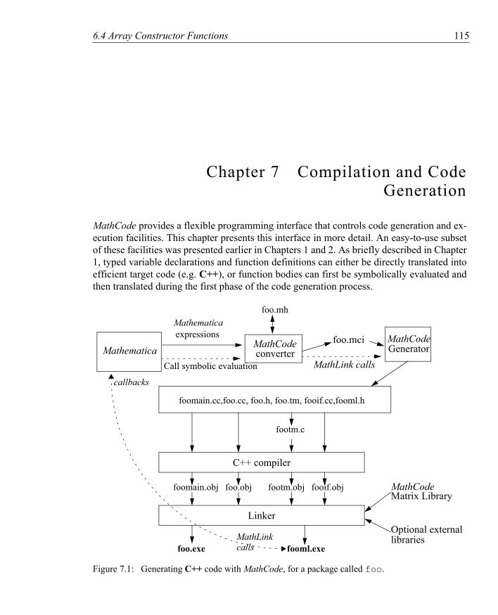
6.4 Array Constructor Functions 115
Chapter 7 Compilation and Code Generation
MathCode provides a flexible programming interface that controls code generation and ex-ecution facilities. This chapter presents this interface in more detail. An easy-to-use subset of these facilities was presented earlier in Chapters 1 and 2. As briefly described in Chapter 1, typed variable declarations and function definitions can either be directly translated into efficient target code (e.g. C++), or function bodies can first be symbolically evaluated and then translated during the first phase of the code generation process.
MathematicaMathCodeGenerator
Mathematicaexpressions
Call symbolic evaluation
foomain.cc,foo.cc, foo.h, foo.tm, fooif.cc,fooml.h
MathCodeconverter
foo.mci
MathLink calls
footm.c
foo.mh
fooif.objfootm.objfoo.objfoomain.obj
fooml.exefoo.exe
C++ compiler
Linker
Matrix LibraryMathCode
Optional externallibraries
callbacks
MathLinkcalls
Figure 7.1: Generating C++ code with MathCode, for a package called foo.
116 7.1 Overall System Structure
7.1 Overall System Structure
Compilation and code generation in the MathCode context can be described from the per-spective of a number of largely orthogonal dimensions. For example, to which type of target code should the Mathematica code be translated? What is the compilation scope, i.e. which parts of the Mathematica program should be translated? Should the Mathematica code be symbolically evaluated as the first step of code generation or not? Should the compiled code be integrated, i.e. be set up to be transparently callable from Mathematica, or should it just be placed in an external file? Others issues concern how to invoke the code generator.
The typical case of generating C++ code from a Mathematica package (e.g. called foo), is depicted in Figure 7.1. Some parts of the MathCode code generator run within Mathematica (MathCode converter), but most of it resides in a separate process called via MathLink (MathCode generator). This is invisible to the user, for whom the code generator appears to be an ordinary Mathematica package.
Partially translated Mathematica expressions analyzed by the MathCode converter are written to the intermediate form in the file foo.mci which is sent over to the external process, MathCode generator. Sometimes the MathCode generator needs to call back to Mathematica to perform symbolic evaluation of expressions. In this case the result of the symbolic evaluation is sent to the MathCode generator via Mathlink calls.
The package foo is translated to C++ code in the file foo.cc, together with the header files foo.h and foolm.h. The latter file contains declarations for MathLink communication. A MathLink template file foo.tm, together with MathLink interfacing code in files fooif.cc are also produced. The mprep tool from the standard Mathematicadistribution is used by MathCode to generate the file footm.c from foo.tm. A main program file foomain.cc is produced for the case when the user wants to build a stand-alone executable from the generated code. The MathCode header file foo.mh is a Mathematica package file which lists all functions generated by MathCode from the package foo and as well as types referenced by those function signatures. The compilation options used when the foo package was compiled to C++ are also stored in the file foo.mh. The information in the MathCode header file is used by InstallCode, and in situations when code is generated for packages using typed functions from other packages.
7.2 Compilation and Code Generation AspectsThere are four main aspects of code generation in MathCode which are largely orthogonal, i.e. they describe independent properties that can be combined in almost any way.
7.2.1 Target Code Type
The target code option specifies which type of code should be produced by the code gener-

7.2 Compilation and Code Generation Aspects 117
ator. The only available choices at this time are C++ and Fortran90, but other options such as Java, or Mathematica byte code might become available in the future.
The code generator produces efficient code in C++ that is often 1000 times faster than inter-preted Mathematica code, or 100 times faster than internally compiled code. Mathematicavector and matrix operations for tensors up to 4 dimensions are translated to C++ code with calls to the highly efficient MathCode C++ array library. The array storage format is directly compatible with well-known Fortran routine libraries such as BLAS, LinPack etc. by using column-major1 storage layout.
7.2.2 Evaluation of Symbolic Operations
Many Mathematica operations are symbolic in nature, i.e. they produce symbolic Mathe-matica expressions. Examples are symbolic integration and differentiation, simplification, substitution of expressions, etc. Such symbolic operations are not useful to translate to strongly typed languages, e.g. C++ or Fortran90, since this would entail reimplementation of a large part of the functionality of a computer algebra system, and would probably not give better performance than the original system.
However, most symbolic operations eventually produce symbolic expressions which are (numerically) computable when symbolic variable names are replaced by data values. This makes it useful to perform all symbolic operations before generating the target code, since the result of the symbolic operations in most cases will be executable expressions without symbolic operations. It is of course also possible to partially evaluate expressions with a mixture of symbolic and numeric operations before passing those on to the code generator.
The code generator is informed about which functions should be symbolically evaluated/expanded in conjunction with code generation by setting the EvaluateFunctions option, see Section 7.3.2 on page 119.
7.2.3 Integration
The integration property determines whether the compiled code will be integrated for direct execution with Mathematica, or whether the generated code should simply be stored in an external file. Such integrated functions are callable in exactly the same way as internal in-terpreted Mathematica functions.
There are several aspects of code integration:
• Compiled code integration. Compiled function definitions can be integrated to be directly callable from Mathematica. Alternatively, they are simply linked into an
1. Future versions of MathCode may provide a choice of row-major or column-major.
118 7.3 Invoking the Code Generator
executable for stand-alone execution.• External code integration. Function definitions in external libraries or software modules
can be integrated to be callable from Mathematica and/or from generated code. • Callbacks. Some Mathematica functions cannot be translated to external code. Such
function calls can be evaluated by callbacks to Mathematica.
7.3 Invoking the Code GeneratorThe code generation facilities can be invoked by calling a number of Mathematica func-tions, defined in the Mathematica package MathCode. Some of these functions are actually just stubs which call corresponding routines in the MathCode code generator process via MathLink. Below we describe the available code generation functions. Note that in all Math-Code functions taking a package argument, the package name can be given with or without backtick (‘).
7.3.1 CompilePackage[]—the Primary Code Generation Function
The function CompilePackage controls the compilation of entire Mathematica packages which contain typed and/or untyped function definitions, variable declarations etc. Howev-er, only typed definitions are compiled. Untyped definitions will be ignored.
CompilePackage[packagename]
This function generates code for a Mathematica package. For example:
CompilePackage["mypackage"]
It can also be called with the customary backtick:
CompilePackage["mypackage‘"]
Note! The package name "mypackage‘" (or "mypackage") refers to the context name rather than the package itself. CompilePackage["mypackage‘"] searches typed vari-ables and function in the context "mypackage‘". CompilePackage["Global‘"] is therefore generating code for all types of variables and functions belonging to the default context "Global‘".
If no package name is provided as an argument to CompilePackage (or toBuildCode, MakeBinary), the most recent package name used in calls to these functions is used as default. The initial default is "Global’". For example:

7.3 Invoking the Code Generator 119
CompilePackage[]
Different Items to be Compiled
CompilePackage compiles the different items in the package as follows:
• Variable declarationsAll typed global variables declared in a Mathematica package to be compiled (e.g. package foo) are translated to declarations in C++. Declarations are put into the header file foo.h and possible initialization code into the file foo.cc.
• FunctionsThe default is to translate typed Mathematica functions into C++ without any symbolic evaluation. This produces target code similar to the original Mathematica code, i.e. loops in Mathematica become loops in C++ etc.
• Functions with symbolic operationsFunctions which contain symbolic operations such as symbolic integration, substitution etc. should be symbolically expanded (see Section 7.5) before final code generation. Those functions should be indicated using the option EvaluateFunctions described in Section 7.3.2 below.
• Main program functionIn the case that a stand-alone executable is to be created, the option MainFileAndFunction described on page 121 can be used to specify the C/C++ function main() needed in such an executable.
7.3.2 Optional Parameters to Control Code Generation
There are several optional parameters to CompilePackage that provide more detailed con-trol over the code generation process. However, instead of passing such parameters to Com-pilePackage it is usually more convenient to set these options via calls to SetCompila-tionOptions which are placed at the beginning of the package to be compiled.
SetCompilationOptions
Additional information needed to guide the compilation process can be specified using op-tional parameters to CompilePackage and/or MakeBinary, or by inserting calls to Set-CompilationOptions within the package to be compiled. Section 7.4 on page 125 shows the recommended placement of such calls.

120 7.3 Invoking the Code Generator
Below we briefly examine the available options.
Priority of Parameter Settings
Options passed directly to CompilePackage and MakeBinary have the highest priority, i.e. they override the settings made via SetCompilationOptions. If a compilation option is cleared, any existing individual attribute settings will apply.
Option EvaluateFunctions
As mentioned above, CompilePackage automatically compiles all typed functions and variables in the package. The default assumption is that those functions should be compiled without symbolic evaluation using CompileFunction.
However, side-effect free function bodies which contain symbolic operations (see Section 7.5 on page 126) should be compiled using CompileEvaluateFunction instead of CompileFunction. The set of functions which should be compiled in this way can be specified using the EvaluateFunctions option. For example:
CompilePackage["mypackage",EvaluateFunctions->{func1,func2}]
or defining SetCompilationOptions in the package context:
mypackage‘SetCompilationOptions[EvaluateFunctions->{func1,func2}]
Option UnCompiledFunctions
This option prevents some typed functions in the package from being compiled. This might be the case for functions which are only meant to be expanded within the body of another symbolically evaluated function. For example:
SetCompilationOptions[UnCompiledFunctions->{sin,cos,arcTan}]
See Section 2.3.5 on page 42 for an example where this option is used.
Option DisabledMathLinkFunctions
This option (used in very rare cases) prevents some typed functions of the package from be-ing called via MathLink. By default all functions in the package given as argument to Make-Binary can be called by MathLink from the Mathematica environment. This option might be useful in the case that the installed MathLink function confuses Mathematica, or if its call template is generated with errors. This is primarily intended as a temporary workaround in case of errors. Example:

7.3 Invoking the Code Generator 121
SetCompilationOptions[DisabledMathLinkFunctions->{foo1,foo2}]
Option CallBackFunctions
This option specifies that certain functions will be available for callback to Mathematicafrom C++. Thus a callback stub function will be produced in the generated code. See Section 7.7.3 on page 132 for more information. An example call:
SetCompilationOptions[CallBackFunctions->{BesselJ, RiemannSiegelZeta,...}]
Option MainFileAndFunction
In the case that a stand-alone executable is to be created, the option MainFileAndFunc-tion can be used to specify the C function main() needed in such an executable. The ar-gument string specifies the text of the main() function in the file foomain.cc. (see sec-tion 7.6.1 regarding the StandAloneExecutable option).For example:
SetCompilationOptions[ MainFileAndFunction->"int main(){return 0;}"]
or
CompilePackage["foo", MainFileAndFunction->"int main(){return 0;}"]
Option ExternalLanguage
This option gives information about the default external language for external function dec-larations within a module. See Section 8.2.4 on page 140. This is an option to SetCompi-lationOptions, ExternalProcedure, and ExternalFunction. Two examples:
SetCompilationOptions[ExternalLanguage->"Fortran"]
... := ExternalFunction[...,ExternalLanguage->"Fortran"]
Option NeedsExternalLibrary
This option informs about the need for external libraries where called external functions may be defined. This is an option to SetCompilationOptions and MakeBinary.
MakeBinary[NeedsExternalLibrary->{"extlib1", "extlib2"}, NeedsExternalObjectModule->{"file3"} ]
122 7.3 Invoking the Code Generator
Option NeedsExternalObjectModule
This option informs about the need for external modules where called external functions may be defined. This is an option to SetCompilationOptions and MakeBinary.
MakeBinary[NeedsExternalObjectModule->{"file3"} ]
Note that an object module fee.obj produced by MathCode corresponding to a package fee that is used (by e.g. calling Needs["fee"]) within another package foo, is automat-ically linked into the binaries for foo by MakeBinaries["foo"], if fee.obj is in the current directory. The option NeedsExternalObjectModule is not needed in that case.
Option InlineFlag
This option causes array access functions, array slice operations and array indexing func-tions to be inlined in the resulting C++ code, which can speed up execution by 20-30% for indexing intensive applications. This option is turned off by default. Turning it on also changes the default setting of RangeCheckFlag to off for maximum performance. If a val-ue for RangeCheckFlag is given explicitly, that value is of course used. C++ compilation usually becomes several times slower (e.g. 1 minute instead of 15 seconds) when Inline-Flag is turned on, due to the use of larger header files. Example:
SetCompilationOptions[InlineFlag->True]
Option RangeCheckFlag
This option controls whether or not range (bounds) checking is performed for every array access. It is very useful during development, as erroneous accesses cause unpredictable re-sults if it is turned off. For maximum performance in the finished application, it should be turned off. The default value for this flag is True if InlineFlag is False, and False if InlineFlag is True. Basically, the use for this flag is to test inlined code with range checking turned on. Example:
SetCompilationOptions[RangeCheckFlag->True]
Option MacroRules
This option specifies a set of rules that are applied to the right-hand side of every function before compilation. Example:
SetCompilationOptions[MacroRules->{Sin[x_]/Cos[x_]->Tan[x_]}]
The above basically causes the following Mathematica replacement rule to be applied to ev-

7.3 Invoking the Code Generator 123
ery function body to yield the code to compile:
funcbody //. {Sin[x_]/Cos[x_]->Tan[x_]}
Option DebugFlag
The option DebugFlag (value True or False) controls whether or not a debugging trace of the code converter is printed. This flag is mainly intended for internal use by the Math-Code developers.
SetCompilationOptions[DebugFlag->True]
Option Language
The Language option (currently only C++ and Fortran90 is supported) controls which tar-get language MathCode will generate code for. MathCode will use the default compiler for the specified language, which is chosen at the installation of MathCode. In order to use a certain language, you need a MathCode license for that language. Examples of selecting the language:
CompilePackage[Language->"C++"]CompilePackage[Language->"C++"]
The system can reject the request if generating code in the chosen language is not permitted by the license check.
Option Compiler
The Compiler option makes it possible to select which compiler should be used to compile generated code in a given target language. The option value should be one of the symbolic names (strings) of compilers defined during MathCode installation and stored in the Math-CodeConfig.m configuration file. The Compiler option to MakeBinary overrides the default compiler specified for the selected language. Example:
MakeBinary[Compiler->"g++"]
As usual, BuildCode[] can be given both CompilePackage[] and MakeBinary[] op-tions. The following example will generate C++ code and use the "CC" compiler to compile this code, overriding any default specification:
BuildCode[Language->"C++", Compiler->"CC"]
124 7.3 Invoking the Code Generator
Option CompilerOptions
CompilerOptions is an option to MakeBinary[]. CompilerOptions->"opts" adds the string "opts" to the set of options given to the C++ compiler. The default value of this option is "". The makefile variable CCOPT in the makefile is assigned the string "opts". The fileMathCodeConfig.m contains a string with the name of the makefile used by MathCodeto produce executable binaries. See also Section 7.6.1 about MakeBinary for further infor-mation. Example:
SetCompilationOptions[CompilerOptions->"-g -w"]
or
MakeBinary["Foo", CompilerOptions->"-g -w"]
This assigns the string "-g -w" as the value of the makefile variable CCOPT, which subse-qently can be used within compilation commands, linking commands, or in the definition of additional makefile variables such as the variable INC below:
INC = $(CCOPT) -I$(LM)/include -I$(LM)/icc -DNOPAR
Option LinkerOptions
LinkerOptions is an option to MakeBinary[]. LinkerOptions->"opts" adds the string "opts" to the set of options given to the linker. The default value of this option is "". The makefile variable LINKOPT in the actual makefile is assigned the string "opts". See also Section 7.6.1 about MakeBinary for further information. An example:
SetCompilationOptions[LinkerOptions->"-lm"]
The option -lm requests linking with libm.a library on Unix systems and for GCC compilers
Option MathCodeMakeFile
MathCodeMakeFile is an option to MakeBinary[] that makes it possible to replace the standard makefile with a user specified one. MathCodeMakeFile->"filename" specifies the makefile template to be used for building the executables. The file MakefileCon-fig.m contains a string with the name of the makefile used by MathCode to produce bina-ries.
MakeBinary["Foo",MathCodeMakeFile->"/home/putte/mymake.mak"]

7.4 Standard Layout of a Package to be Compiled 125
This command results in the use of the makefile mymake.mak instead of the default make-file.
7.4 Standard Layout of a Package to be CompiledBefore going into more detail about code generation we present the layout of a typical Math-ematica package (named by the dummy name foo) to be compiled by MathCode. All ex-ample packages in Chapter 2 have this structure.
The call to SetCompilationOptions regarding functions is best placed after the sections for public names and package global names since those names need to be declared first, as in the example package foo below. The information about external libraries, on the other hand, can be specified in the same place or closer to the beginning of the package. Note that the object module for fee1.obj is automatically passed to the linker if the package fee1 has been compiled before.
The typical recommended package layout is as follows:
Needs["MathCode‘"]
BeginPackage["foo‘",{MathCodeContexts,"fee1‘",...}]...
(* Possible need for external libraries or object code *)SetCompilationOptions[NeedsExternalLibrary->{"extlib1","extlib2"}, NeedsExternalObjectModule->{"extmodule1"} ]
(* Public, exported names *)...
(* Private, package-global names *)...
(* Possible setting of compilation options for certain functions*)SetCompilationOptions[EvaluateFunctions->{func1,func2}];...
(* Private implementation section *)Begin["‘foo‘Private"]...
End[];EndPackage[];

126 7.5 Code Generation of Symbolically Evaluated Expressions
7.5 Code Generation of Symbolically Evaluated ExpressionsThe following example illustrates code generation for (usually very large) symbolic expres-sions that are created by Mathematica during symbolic evaluation when calling Com-pilePackage with the EvaluateFunctions option. Common subexpression elimina-tion is performed on such code in order to break it into pieces and to make it execute more efficiently.
Common Subexpression Elimination
The code generator takes advantage of the fact that pure (i.e. side-effect free) functions like sin, cos, and tan are devoid of side-effects in order to eliminate common subexpressions that the C++ compiler sometimes cannot optimize since it normally cannot assume that all li-brary functions are side effect free. Note that it is necessary to eliminate all common subex-pressions (even if the compiler can handle the ones involving only arithmetic operators) so that we do not miss any opportunities for further optimizations. Temporary variables which hold the results of subexpressions are also introduced. Thus the code generator must derive the type of each subexpression, including the types of intermediate arrays.
Even without the common subexpression elimination, some partitioning of the symbolic expressions would be necessary since the expressions may otherwise become so large that the target language compiler cannot handle them—many compilers have a built-in hard limit on the size of expressions.
A Short Example
As an example, consider the following Mathematica function. func[Real a_] -> Real :=
Cos[a+5] * Sin[a]*Sin[a+5] + Sin[a]*Cos[a]*Cos[a]*(a+5); The code generator invoked by
CompilePackage[EvaluateFunctions->{func}].
The following C++ code is generated:
double Global_Tfunc ( const double &a){ double mc_T1; double mc_T2; double mc_T3; double mc_T4; double mc_T5;

7.6 Building Executables 127
double mc_T6; double mc_T7; double mc_T8; double mc_T9; mc_T1 = 5+a; mc_T2 = sin(mc_T1); mc_T3 = sin(a); mc_T4 = cos(mc_T1); mc_T5 = mc_T4*mc_T3*mc_T2; mc_T6 = cos(a); mc_T7 = (mc_T6*mc_T6); mc_T8 = mc_T1*mc_T7*mc_T3; mc_T9 = mc_T8+mc_T5; return mc_T9;}
The only common subexpressions in this example are 5+a (stored in mc_T1 and used three times) and Sin[a] (stored in mc_T3 and used twice). For complicated expressions in re-alistic applications, the common subexpression elimination often reduces the size of the generated code by a factor of ten or more.
Different numerical programs can be generated from the same Mathematica program depending on how much information is supplied before generating and compiling the code. If Mathematica variables are declared as constants and initialized to constant numerical values before such code generation, symbolic simplification usually results in a more efficient but less general program. This can be viewed as a form of partial evaluation of the program.
7.6 Building ExecutablesThe building process compiles all produced C++ files and links them into one (or two) ex-ecutables. An overview is presented in figure 7.2
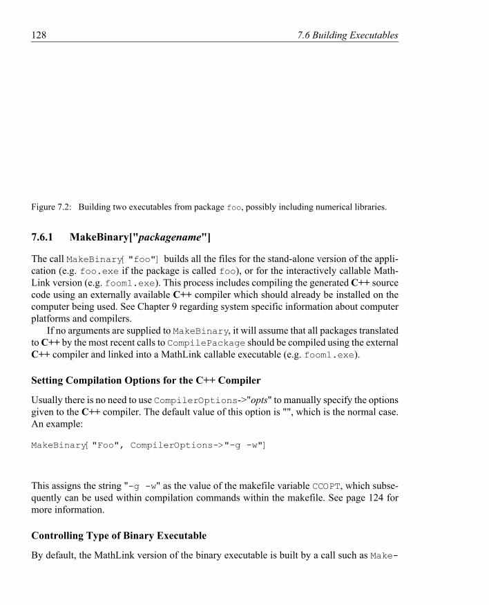
128 7.6 Building Executables
foo.exeNumerical
Package(s)fooml.exe
foo.ccfoo.hfoomain.ccfootm.cfoo.tm
Library
fooif.cc
Figure 7.2: Building two executables from package foo, possibly including numerical libraries.
7.6.1 MakeBinary["packagename"]
The call MakeBinary["foo"] builds all the files for the stand-alone version of the appli-cation (e.g. foo.exe if the package is called foo), or for the interactively callable Math-Link version (e.g. fooml.exe). This process includes compiling the generated C++ source code using an externally available C++ compiler which should already be installed on the computer being used. See Chapter 9 regarding system specific information about computer platforms and compilers.
If no arguments are supplied to MakeBinary, it will assume that all packages translated to C++ by the most recent calls to CompilePackage should be compiled using the external C++ compiler and linked into a MathLink callable executable (e.g. fooml.exe).
Setting Compilation Options for the C++ Compiler
Usually there is no need to use CompilerOptions->"opts" to manually specify the options given to the C++ compiler. The default value of this option is "", which is the normal case.An example:
MakeBinary["Foo", CompilerOptions->"-g -w"]
This assigns the string "-g -w" as the value of the makefile variable CCOPT, which subse-quently can be used within compilation commands within the makefile. See page 124 for more information.
Controlling Type of Binary Executable
By default, the MathLink version of the binary executable is built by a call such as Make-
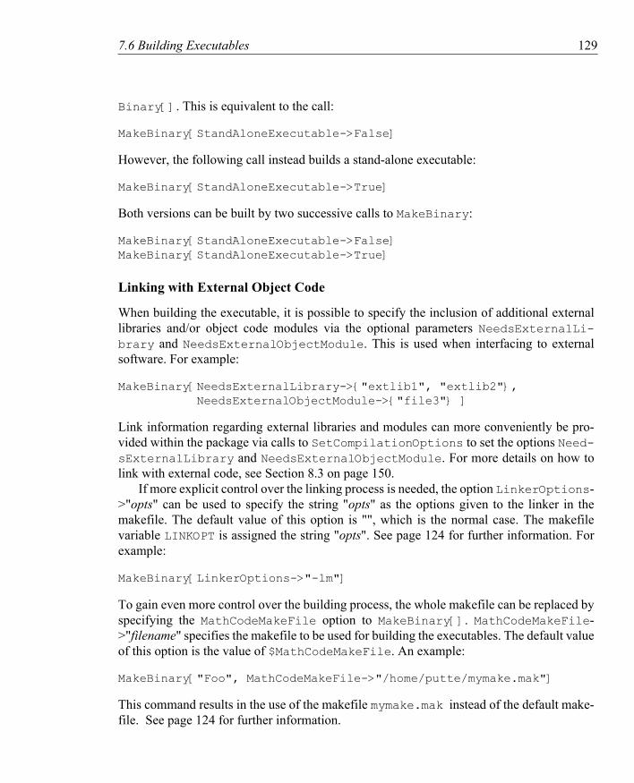
7.6 Building Executables 129
Binary[]. This is equivalent to the call:
MakeBinary[StandAloneExecutable->False]
However, the following call instead builds a stand-alone executable:
MakeBinary[StandAloneExecutable->True]
Both versions can be built by two successive calls to MakeBinary:
MakeBinary[StandAloneExecutable->False]MakeBinary[StandAloneExecutable->True]
Linking with External Object Code
When building the executable, it is possible to specify the inclusion of additional external libraries and/or object code modules via the optional parameters NeedsExternalLi-brary and NeedsExternalObjectModule. This is used when interfacing to external software. For example:
MakeBinary[NeedsExternalLibrary->{"extlib1", "extlib2"}, NeedsExternalObjectModule->{"file3"} ]
Link information regarding external libraries and modules can more conveniently be pro-vided within the package via calls to SetCompilationOptions to set the options Need-sExternalLibrary and NeedsExternalObjectModule. For more details on how to link with external code, see Section 8.3 on page 150.
If more explicit control over the linking process is needed, the option LinkerOptions->"opts" can be used to specify the string "opts" as the options given to the linker in the makefile. The default value of this option is "", which is the normal case. The makefile variable LINKOPT is assigned the string "opts". See page 124 for further information. For example:
MakeBinary[LinkerOptions->"-lm"]
To gain even more control over the building process, the whole makefile can be replaced by specifying the MathCodeMakeFile option to MakeBinary[]. MathCodeMakeFile->"filename" specifies the makefile to be used for building the executables. The default value of this option is the value of $MathCodeMakeFile. An example:
MakeBinary["Foo", MathCodeMakeFile->"/home/putte/mymake.mak"]
This command results in the use of the makefile mymake.mak instead of the default make-file. See page 124 for further information.

130 7.7 Integration
7.6.2 BuildCode["packagename"]
The call BuildCode["foo"] calls CompilePackage["foo"] and then MakeBina-ry["foo"], i.e. a call to BuildCode["foo"] will make a complete code generation, compilation and linking of the Mathematica package "foo‘".
BuildCode["foo"]
7.7 IntegrationAs already mentioned, the integration property determines if compiled or external code will be integrated for direct execution with Mathematica. Such integrated functions are callable in exactly the same way as internal interpreted Mathematica functions.
7.7.1 Calling Compiled Generated Code via MathLink
Integrated functions are compiled and linked into an executable, e.g. as fooml.exe in Figure 7.3 below, which is connected to Mathematica via MathLink.
Generated code to be executed stand-alone, i.e. in a non-integrated fashion, is linked into a stand-alone executable, for example foo.exe in Figure 7.3.
foo.exe
MathematicaNeeds["foo‘"]
fooml.exeMathLink
Figure 7.3: Integrating generated code from the package foo with Mathematica. Functions in fooml.exe can be called interactively from Mathematica via MathLink. The binary file foo.exe can be used for non-integrated stand-alone execution.
The following MathCode functions control the integration of compiled code with Mathe-matica. It is possible to switch back and forth between executing the compiled versions of Mathematica functions and the original interpreted versions by successively calling Acti-vateCode[] and DeactivateCode[]. This is useful for testing purposes and perfor-

7.7 Integration 131
mance comparisons. The names of both interpreted and compiled functions are always kept within the original context.
Only the functions within the package specified as an argument to MakeBinary or BuildCode will be made callable via MathLink. If multiple compiled packages are linked together, functions in other packages are currently not made automatically available via MathLink. The workaround is to insert stub functions into the main package whose only purpose is to call those functions you want to access interactively.
• InstallCode[]. Installs compiled code for possible execution from within Mathematica through stub functions for calls via MathLink. MathLink stub1 functions to generated code are stored under ExternalDownValues. Each interpreted function definition in the relevant package is moved from DownValues[funcname] to SourceDownValues[funcname]. Then an ActivateCode[], see below, is performed. Thus, InstallCode[] performs the following actions:– Reads the MathCode header file corresponding to the package, to find the list of
functions for which there is external code generated and compiled.– Saves interpreted function definitions for the relevant functions under
SourceDownValues, and clears DownValues for these functions.– Performs Mathematica Install[] if the generated code is callable via MathLink,
and saves the stub functions under ExternalDownValues[]. – Saves the MathLink descriptor to the open MathLink connection, so that it can be
closed later by UninstallCode[]. In the case of compiled bytecode this is not necessary.
• ActivateCode[]. When the compiled code is activated, the interpreted function definitions are removed and saved under SourceDownValues[funcname] for each function. Instead the compiled function definitions are activated for possible execution by setting DownValues[f] to ExternalDownValues[f].
• DeactivateCode[]. Deactivates previously installed and activated compiled code, by restoring the interpreted function versions if available, i.e. resetting DownValues to SourceDownValues.
• UninstallCode[]. First perform a DeactivateCode[]. Then close possible open MathLink connections and remove MathLink stub functions.
1. A stub function is an interface function that performs no action of its own apart from possibly re-ordering/re-packaging the function arguments before passing them on to the function that performs the actual work.
132 7.7 Integration
Code Storage Places
Where is compiled Mathematica code stored? We have already seen (Figure 7.1) that gen-erated code in languages like C++ or Fortran90 is placed in external files, which are then further compiled and linked into a binary executable file.
However, internal storage places within Mathematica are needed both for storing the original interpreted definitions of compiled Mathematica functions, the stub functions needed for possible communication with compiled code via MathLink, and compiled bytecode in case Mathematica functions are compiled to bytecode. Information about these storage places is not necessary to know in order to use MathCode, but might be of some help for the advanced Mathematica programmer.
The following code storage places are employed by MathCode within Mathematica:
• DownValues. The currently active definition rules for a Mathematica function f are obtained through DownValues[f], or assigned by DownValues[f]=...
• SourceDownValues. The standard interpreted Mathematica source versions of the functions are saved here when the interpreted versions are replaced by stub functions or compiled versions.
• ExternalDownValues. Function definitions which are ExternalCall expressions calling external executable code via MathLink. ExternalCall is a built-in Mathematica function used to call external MathLink objects.
7.7.2 Integration of External Libraries and Software Modules
The integration of external software means that external code, available in libraries or object modules and originally implemented in languages like Fortran, C, C++, is integrated with the Mathematica execution environment so that functions in the external code can be trans-parently called from within Mathematica. Such code is typically implemented manually and has not been generated by the MathCode code generator. See Section 8.4 on page 151 for a description of how to integrate external code. See Section 7.7.1 regarding interactive calling via MathLink for functions in other modules than the main module.
7.7.3 Callbacks to Mathematica
The ability to perform callbacks to Mathematica functions from external code is especially valuable for compiled code that is set up for execution external to Mathematica for efficien-cy or other reasons, but which may contain calls to internal Mathematica functions that can-not be made available externally, or would be very impractical to re-implement externally. Examples of such functions are some of the special mathematical functions available within Mathematica, e.g. BesselJ, RiemannSiegelZeta, HyperGeometric1F1, etc. Other
7.7 Integration 133
examples are Mathematica graphics functions such as Plot3D, which, however, have very special parameter structures since iterators can be provided as arguments and thus should be called via some intermediate Mathematica function. A common use of these functions is to call Mathematica graphics from external programs.
The type information needed by the code generator to be able to generate callback stub functions in C++ is precisely the type signatures that are specified for all typed Mathematicafunctions. The interface information is the same—the only difference is that calls are made in the opposite direction.
Unfortunately, built-in Mathematica functions, as well as most user-defined functionsnot aimed for compilation, lack this type information, which therefore has to be provided by calling Declare for such functions. For example, the signature of BesselJ might be specified as follows:
Declare[BesselJ[Integer n_, Real z_]->Real ]
The code generator must also be informed that a function is callable from C++ as a callback. This is done by SetCompilationOptions (see page 119) which can be called within the package to set the option CallBackFunctions for one or more functions. For example:
SetCompilationOptions[ CallBackFunctions->{BesselJ,RiemannSiegelZeta} ]
Below is the function interface prototype of the generated stub function in C/C++ for BesselJ:
double BesselJ(int n, double z);
Example call in C/C++:
z1 = BesselJ(2, 3.54)
Errors in Callbacks
If there is a risk that errors may occur within the callback function, or that non-numeric C++-incompatible results may be returned, it may be advisable for the user to define his or her own callback function which calls the desired function and performs extra error check-ing. Otherwise, if an appropriate value is not returned by the callback via Mathlink, the Mathlink connection will enter an inconsistent state which makes it unusable. For example:
MyBesselJ[Integer n_, Real z_]->Real := Module[{result,...}, ... (parameter error checking code) ...

134 7.8 Providing Missing Mathematica Functions
result = BesselJ[n,z]; ... (result error checking code) ... result];
Placement of Generated Callback Stub Functions
The generated C++ callback stub functions are normally placed in the generated code file corresponding to the Mathematica package context of the function symbol.
For example, the C++ stub function for foo‘MyBesselJ will be placed in the file foo.cc when the package foo is compiled if foo‘MyBesselJ has been specified in the list associated with the CallBackFunctions compilation option as described on page 121.
Generated callback stub functions of Mathematica system functions, most of which originally reside in the System package, are either placed in the file system.cc or in an application file such as foo.cc, according to where calls like SetCompilationOptions[ CallBackFunctions -> {func1, func2,...}] are placed:• In system.cc. This is the case if the function symbol has the system context mark,
e.g. system‘BesselJ, which occurs if the callback settings are done in the systempackage.
• In an application file. This placement is useful when it is undesirable to change the system file, for example when dealing with rarely used callbacks only called within a specific application package. By setting the option CallBackFunctions for that package, either via SetCompilationOptions or via the actual call to CompilePackage, generated callback stubs will be placed in the produced C++ application file regardless of the context marks of the callback function symbols.
7.8 Providing Missing Mathematica FunctionsThe MathCode translator directly supports a set of basic Mathematica functions and opera-tions, as defined in Appendix A. There are still a number of standard Mathematica functions not yet included in this set. Basically three ways of providing implementations of missing standard functions exist:
• Callback. Standard Mathematica functions can be made callable from external code, by providing callback declarations (see section 7.7.3). This is easy, but usually gives low performance because of the MathLink communication overhead and interpreted evaluation within Mathematica.
• Re-implementation. Standard functions can be re-implemented by hand, semi-
7.9 Code Compilation from Command Shell 135
automatically by generating an external interpolating function version of the Mathematica function in question, or by using available external implementations e.g. from a library. This process is simplified by the availability of the system package described below.
• User-defined macros. Functions can be defined by macros/replacement rules passed as an option to CompilePackage, see Option MacroRules on page 122.
7.8.1 The system Package
The user can supply his or her own implementations of missing functions by providing al-ternative Mathematica function implementations in the system package. It is intentionally named system (lower-case!) to mimic the Mathematica System context which contains most standard functions. The system package is by default translated and, if needed, in-cluded in built executables.
The available array slice operators in MathCode simplify re-implementation of certain list-operations, which are not directly supported by MathCode but are indirectly supported as array slice operators.
The object module system.obj (system.o under Unix) is included by default when linking executables if the compiled package uses a Mathematica function not in the compilable subset of MathCode but implemented in the system package. However, the intention is to use the system for such standard functions which have already been implemented and tested. This is to avoid unnecessary recompilation of already implemented functions while the user is developing implementations of additional functions. At delivery, the MathCode system contains a system package and a system object module containing a number of Mathematica functions which have been re-implemented in this way.
The header file system.h is automatically included, if needed, in produced C++ code so that system functions can be called from generated code. Additionally, the code generator performs the special action of creating MathCode header files when compiling system. This file, which is always loaded when MathCode is started, is called system.mh, and contains only typed Mathematica external declarations of the compiled functions.
An example of a system package is provided as a system.nb notebook file. It currently resides in "MathCode/lib/stdpackages/src/". See UsingSystem.nb demo which explains how functions from System.nb should be used. The contents of this file depend on MathCode version, used language (C++ or Fortran) and attached libraries.
7.9 Code Compilation from Command ShellInstead of using MakeBinary[] call every time, you can also use the standard command shell for compilations.
136 7.9 Code Compilation from Command Shell
7.9.1 Command Shell Compilation in Windows using make
MakeBinary creates the command script named packagename.cmd. The shell command:
make -f packagename.cmd
invokes the make utility, which in turn invokes the C++ compiler and linker.
7.9.2 Command Shell Compilation in Windows using nmake
The shell command:
nmake @packagename.cmd
invokes the nmake utility, which in turn invokes the C++ compiler and linker. Either the stand-alone or the MathLink version of the executable file is created depending on the set-ting of the option StandAloneExecutable. System requirements are described in the MathCode distribution.
7.9.3 Command Shell Compilation in UNIX
MakeBinary creates the make file packagename.unx. The UNIX command
make -f packagename.unx
invokes the make utility, which in turn invokes the C++ compiler and linker. Either the stand-alone or the MathLink version of the executable file is created depending on the set-ting of the StandAloneExecutable option. UNIX system requirements are described in the MathCode distribution.
137
Chapter 8 Interfacing to External Libraries
The MathCode system makes it possible to call functions in generated code from within Mathematica or from generated code. However, there is also a need to directly call external functions which may be available in external libraries and have often been implemented in languages such as Fortran, C, or C++. Interfacing to external code is useful in many situa-tions, for example the following:• Interfacing to Fortran numeric libraries, e.g. LinPack, IMSL, BLAS, etc.• Integrating with simulation applications, robotics etc.• Interfacing to graphics libraries such as OpenGL.
External functions reside in executable form within some external process, and can be called from within Mathematica via Mathlink, or directly from within generated code that has been translated, compiled, and loaded into the external process.
8.1 External VariablesAn external variable denotes a data structure, e.g. a matrix, that is declared to be created only outside the Mathematica workspace, for example within an external process into which translated C++ code is downloaded. External functions which reside within this external ad-dress space can operate directly on these external data structures. This makes sense for large data structures such as million element arrays, which can be created and operated on much more efficiently in the external representation than within Mathematica.
However, external variables cannot be accessed interactively via MathLink from within Mathematica, except indirectly through possible user-defined access functions.
8.2 External FunctionsThe most important aspect of external functions is the interfacing problem—how to transfer parameters at function call and obtain results at function return.

138
Mathematica function parameters are essentially always input parameters. This is standard among functional programming languages. Arguments are usually evaluated before being passed to the called function, i.e. call by value. This excludes Mathematicafunctions with non-standard evaluation order, which are not considered here. Mathematicafunctions may return multiple results as a “function value” consisting of a set of results, which is also the case for most other functional languages.
By contrast, common imperative languages such as C, C++, Fortran, etc. allow function parameters to return results by passing arguments by reference. Such parameters can be used as Output or InOut parameters. In the InOut case, a value is first passed in via the parameter, and a result is later returned out via the same parameter.
Thus, we need a mechanism to call external functions from Mathematica, allowing Input, Output and InOut parameters, while preserving the nice functional style of Mathematica function invocation. Even though there are special cases where call by reference can be emulated in Mathematica, we want to avoid such solutions since they are non-functional in style and generally unapplicable.
8.2.1 Data Transfer at Function Call
The most important property to specify is how data is transferred into or out of the external function via function values and/or parameters.
From a data flow point of view, there are three kinds of external function parameters:
• Input. Data flows into the external function parameter at function call.• Output. Data flows out from the external function parameter when the function returns.• InOut. Data flows into the parameter at call time, and then out from the parameter at
function return time.
Input is default, and therefore usually not specified in external declarations. Other relevant properties of the external function interface are:
• Function value. The external function may or may not return a value — i.e. it is either a function or a procedure.
• Inputs only. The external function has Input parameters only.• Inputs; Outputs. There are Input parameters followed by some Output parameters at the
end of the parameter list.• Mixed. Mixed Input, Output or InOut parameters occur at arbitrary positions in the
parameter list.
139
8.2.2 Mapping External Function Interfaces to Mathematica
An InOut parameter is expected to contain some input data at function call time, and to re-turn an output result when the function returns. Each external InOut parameter gives rise to one Mathematica input parameter and one output function result. InOut parameters are ref-erence parameters in languages like C, C++ and Fortran.
The following simple rules state how external function interfaces are mapped into typed Mathematica function interfaces:
• External function Input or InOut parameters are transferred to the parameter list of the corresponding Mathematica function.
• Each external Output or InOut parameter gives rise to a corresponding result in the Mathematica function result list. Note that external Output parameters are not transferred to the Mathematica version of the function parameter list.
• If there is an external function value, it appears first in the Mathematica function result list, or as the only result if there is just one function result.
These rules have the following consequences regarding function values.
• If there is just one external function result and no Output or InOut parameters, this value is returned as a function value also by the Mathematica function.
• If there are two or more Mathematica function results, this corresponds to an external function with one function value and one or more Output/InOut parameters, or an external procedure or subroutine, i.e. a function with no function value (e.g. voidfunctions in C/C++), with two or more Output parameters and no result.
8.2.3 ExternalFunction and ExternalProcedure Declarations
External functions which are to be called from Mathematica need to be made visible via an ExternalFunction or ExternalProcedure declaration. This is like a normal function declaration, except that the body is replaced by ExternalFunction[] or External-Procedure[] with optional parameters to be described in subsequent sections. The decla-ration has the following general structure, where ExternalFunction should be replaced by ExternalProcedure when the external function is a subroutine or a function with no value (e.g. void in C):
extfunction[type1 arg1_, type2 arg2_,...]->{ftype1,...} := ExternalFunction[];
Note that this declaration does not create a function definition for extfunction with the body ExternalFunction[], as would be the normal behavior of the Mathematica := op-
140
erator. Its primary purpose is to declare necessary type and interface information, which is stored elsewhere when the declaration is evaluated, and may give rise to a MathLink stub function when the package is compiled. The symbol extfunction is created, and tempo-rarily defined as a function that simply returns an error message, until the external function has actually been installed and connected via MathLink.
The package that contains such external declarations needs to be compiled by CompilePackage and installed, before it is possible to call the external functions from within Mathematica.
The information in these external declarations is used in different ways by the MathCodesystem, depending on where the call to the external function occurs:
• Call from C++. The call occurs from within a function body in generated C++ code. MathCode will emit a function interface prototype at the beginning of the generated fileand translate each call to the external function appropriately.
• Call via MathLink. The call occurs in Mathematica and is connected to the external function via MathLink. MathCode will emit a MathLink template, possibly generate code as needed to handle Output/result parameters, and perform other actions needed to automatically create a MathLink executable.
8.2.4 Specification of External Function Language
The MathCode system sometimes needs information about the implementation language of external library functions, especially if they are not written in the current target language emitted by the code generator (here C++), which is the assumed default implementation lan-guage for external code. The language can be specified via the optional ExternalLan-guage parameter to ExternalFunction or ExternalProcedure, placed at the end of the external parameter list if present:
... := ExternalFunction[...,ExternalLanguage->"Fortran"]
... := ExternalProcedure[...,ExternalLanguage->"C++"]
... := ExternalProcedure[...,ExternalLanguage->"C"]The currently supported values of the ExternalLanguage option are "Fortran", "C"
and "C++" (default). The "C++" option can be used for external C code, except when passing arrays which are represented by the addresses of their storage areas and for which dimension size information should be passed as extra parameters instead of being part of the array object.
141
8.2.5 Examples
The different properties of external functions have to be mapped onto a Mathematica func-tion interface restricted to Input parameters and one or more results. In the following we present a number of examples of external functions, where most combinations of relevant properties can be found.
External Input Parameters, no External Function Value
In this case all parameters to the external function are Input parameters. There is no returned function value from the external function, which therefore is declared as an external proce-dure.
The following is an example declaration of such an external function interface in typed Mathematica. Since there is no return type (Null) the external function has type void:
foo[Real x_, Integer y_]->Null := ExternalProcedure[];
Function interface prototype in C++:
void foo(const double & x, const int & y);
Call in Mathematica:
foo[2.4, 3];
Translated call in C++:
foo(2.4, 3);
External Input Parameters, External Function Value
As in the previous case, all parameters to the external function are Input parameters. One function value is returned. This case of external functions directly corresponds to the stan-dard style of functions in Mathematica.
Since there is only one function value, it is by default assumed to be returned as a function value (instead of possibly an Output parameter) by both the external and the Mathematica version. An example:
foo[Real x_, Integer y_]->Real := ExternalFunction[];
External function interface prototype, e.g. in C++:
double foo(const double & x, const int & y);

142
Example call in Mathematica:
z = foo[2.4, 3];
Translated call in C++:
z = foo(2.4, 3);
Default External Output Parameters, no Value
In this case the external procedure returns results through Output parameters, but has no function value. These Output parameters occur at the end of the external function parameter list.
In this example, we do not specify any names of Output parameters in the external declaration. The two results will correspond to two Output reference parameters automatically placed at the end of the parameter list, with default names mc_O1 andmc_O2.
foo[Real x_, Real y_]->{Real, Integer} := ExternalProcedure[];
Generated function interface prototype in C++:
void foo(const double &x, const int &y, double &mc_O1, int &mc_O2);
Example call in Mathematica:
{z1,i2} = foo[2.4, 3];
Translated call in C++:
foo(2.4, 3, z1, i2);
8.2.6 Examples of Fortran and C functions
Named External Output Parameters, External Procedure
In the previous case the MathCode system produced default names mc_O1 and mc_O2 for the Output parameters. The user can also explicitly specify the names and placement of the Output parameters as below. However, in the example below this is not really necessary since the actual names in an external function interface prototype in C are not important for making a correct function call—only the types and placement of parameters really matter.
143
foo[Real x_,Integer y_]->{Real, Integer}:= ExternalProcedure[x, y, Output u1, Output u2];
The following function interface prototype is generated for the external C function:
void foo_(double x, int y, double *u1, int *u2);
If the external language had been Fortran771, this prototype would have been generated:
void foo_(double *x, int *y, double *u1, int *u2);
The call in Mathematica appears as before:
{z1,i2} = foo[2.4, 3];
The translated call in generated C++ code is, of course, done from C++. Hence a prototype for an interface function in C++ must also be generated, which for the above example ap-pears as follows:
void foo(double x, int y, double & u1, int & u2);
The call as translated into C++:
foo(2.4, 3, z1, i2);
Arbitrary Placement of External Output Parameters
The Output parameters in the external function might be placed in a different order than at the end of the parameter list. For example:
foo[Real x_,Integer y_]->{Real, Integer}:= ExternalProcedure[x, Output u1, y, Output u2, ExternalLanguage->"C"];
Function interface prototype in C:
void foo_(double x, double *u1, int y, int *u2);
This is what the prototype would have looked like if ExternalLanguage->"Fortran"had been specified:
1. The link symbol conventions may vary between Fortran compilers. For example, when linking to object code compiled by Digital Fortran under Windows95/NT the synthetic name for the Fortran prototype will be the function name in capital letters (e.g. FOO) in-stead of the function name with a trailing underscore (e.g. foo_). Check README for more information about which compilers are supported in your MathCode installation.

144
void foo_(double *x, double *u1, int *y, int *u2);
Example call in Mathematica:
{z1,i2} = foo[2.4, 3];
The function prototype used for the C++ interface function appears as follows:
void foo(double x, double & u1, int y, int & u2);
Translated call in C++:
foo(2.4, z1, 3, i2);
External InOut/Reference Parameters, External Procedure
There might also be InOut parameters in the external function parameter list. An InOut pa-rameter is expected to contain some input data and a function call time, as well as to return an output result when the function returns. Each external InOut parameter gives rise to one Mathematica Input parameter and one Output function result. InOut parameters are refer-ence parameters in languages like C, C++ and Fortran.
If the parameter u1 in the previous example were an InOut parameter, the type signatures, function interface prototypes, and calls would appear as follows:
foo[ Real x_, Real u1_, Integer y_] -> {Real, Integer} := ExternalProcedure[ x, InOut u1, y, Output u2, ExternalLanguage->"Fortran"];
Function prototype in C for the external Fortran function:
void foo_(double *x, double *u1, int *y, int *u2);
This is what the function prototype would look like if the external language were C instead of Fortran:
void foo_(double x, double *u1, int y, int *u2);
Example calls in Mathematica:
{z1,i2} = foo[536.8, z1, 33];
145
{z3,i4} = foo[2.4, 5.55, 3];
Translated calls in C++:
foo(536.8, z1, 33, i2);
z3 = 5.55;foo(2.4, z3, 3, i4);
A simpler example of an external C++ function foo2 with an InOut reference parameter x2:
foo2[Real x2_,]->Real:= ExternalProcedure[InOut x2];
Example call in Mathematica:
x2 = foo2[x2];
Translated call in C++:
foo2(x2);
8.2.7 Calling External Fortran Library Functions
It is especially important to remember to specify the implementation language when calling functions in external Fortran libraries since Fortran uses reference parameters and Mathe-matica, C, and C++ mostly use call by value parameters, at least for scalar variables.
The solution used by the MathCode translator is to create a wrapper routine and always pass addresses of variables, and to create temporary variables when passing values of constants or expressions. For example, assume that there is a call to the Fortran subroutine FOO, which appears in Mathematica as in previous examples:
{z1,z2} = foo[2.4, 3];
As usual, the external function interface must be specified by the user:
foo[Real x_, Integer y_]->{Real, Real} := ExternalProcedure[ x, y, Output u1, Output u2, ExternalLanguage->"Fortran"];
To make the call possible in the generated C++ code, the following function interface is gen-erated by MathCode to provide a wrapper routine in C++.
146
extern "C" { void foo_(int* x, int* y, double* u1, double* u2);}
C++ stub function:
void foo(double &x, int &y, double &u1_OUT, double &u2_OUT) { foo_(&x, &y, &u1_OUT, &u2_OUT);};
A call to the C wrapper for the Fortran subroutine would need two temporaries because of the call by reference. However, the C/C++ compiler is able to create these automatically (but usually produces a warning), which makes it possible for MathCode to emit the following call:
foo(2.4, 3, z1, z2);
8.2.8 Passing Array Parameters to External Functions
Passing multi-dimensional array parameters to external functions poses special problems since the array representation may vary between different languages, and may not even be standardized within a single language, as in the case of C++.
A common problem in several languages, including C and Fortran77, is that thedimension sizes of array data structures are not part of the data structures themselves. Such information is instead stored in separate variables and passed as extra integer parameters at function calls.
We examine solutions for the three external languages C++, Fortran77 and C. This requires specifying the external language via the ExternalLanguage optional parameter.
Passing Array Parameters to External C++ Functions
The representation of multi-dimensional arrays is not yet standardized in C++. Therefore we assume that the external C++ code uses the MathCode array package, which also makes it compatible with code produced by the MathCode code generator. This is useful when inter-facing hand-implemented C++ functions based on the MathCode array library to Mathemat-ica code or generated code. In the example below the specification ExternalLanguage->"C++" is not necessary since it is assumed to be default if nothing is specified.
foo[ Real[n_] x_, Real[n_,m_] y_, Integer i_] -> {Real[n], Real[_]} :=

147
ExternalProcedure[ExternalLanguage->"C++"];
The function interface prototype is presented below as it appears in automatically generated C++ code which uses the MathCode array library, including the default Output parameters mc_O1 and mc_O2 which return the two results from the Mathematica stub function.
void foo ( const doubleN &x, const doubleNN &y, const int &i, doubleN &mc_O1, doubleN &mc_O2)
An example call in Mathematica, where both z1 and z2 are one-dimensional arrays:
{z1,z2} = foo[{2.4, 3.5}, {{5.55},{3.44}}, 3];
A translated call in C++ below, assuming that tmpvec1 contains the vector {2.4, 3.5}and tmpmat2 contains the array {{5.55}, {3.44}}. The dimension sizes of these arrays are embedded in the array data structures passed, and need not be passed as separate param-eters.
foo(tmpvec1, tmpmat2, 3, z1, z2);
Passing Array Parameters to External Fortran77 Functions
Most available standard numerical libraries are implemented in Fortran77, which is a subset of Fortran90. Also, the representation of multi-dimensional arrays is standardized in Fortranand corresponds to the column-major array storage layout already provided by the C++ MathCode array library, which makes calling Fortran functions very efficient.
In Fortran77 the dimension sizes can be passed as integer parameters, which can then be used to declare array parameters and local arrays with the right dimensions within the Fortran subroutine. However, these additional integer parameters have to be specified in the external parameter list, as in the example below. All array parameters are passed as addresses of the corresponding array storage areas, (not the address of the array descriptors used in the MathCode array library), since all parameters are passed by reference in Fortran.
It is important to know the types, ranks, and roles (Input, Output, or InOut) of the parameters to the Fortran code. Remember that a Fortran InOut parameter is a parameter with two roles: it receives some input when the subroutine is called, and it passes a result back.
For instance:
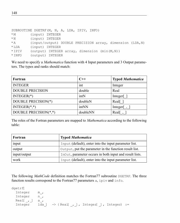
148
SUBROUTINE DGETRF(M, N, A, LDA, IPIV, INFO)*M (input) INTEGER*N (input) INTEGER*A (input/output) DOUBLE PRECISION array, dimension (LDA,N)*LDA (input) INTEGER*IPIV (output) INTEGER array, dimension (min(M,N))*INFO (output) INTEGER
We need to specify a Mathematica function with 4 Input parameters and 3 Output parame-ters. The types and ranks should match:
Fortran C++ Typed MathematicaINTEGER int IntegerDOUBLE PRECISION double RealINTEGER(*) intN Integer[_]DOUBLE PRECISION(*) doubleN Real[_]INTEGER(*,*) intNN Integer[_,_]DOUBLE PRECISION(*,*) doubleNN Real[_,_]
The roles of the Fortran parameters are mapped to Mathematica according to the following table:
Fortran Typed Mathematicainput Input (default), enter into the input parameter list. output Output, put the parameter in the function result list.input/output InOut, parameter occurs in both input and result lists.work Input (default), enter into the input parameter list.
The following MathCode definition matches the Fortran77 subroutine DGETRF. The three function results correspond to the Fortran77 parameters a, ipiv and info.
dgetrf[ Integer m_, Integer n_, Real[_,_] a_, Integer lda_] -> {Real[_,_], Integer[_], Integer} :=

149
ExternalProcedure[ m, n, InOut a, lda, Output ipiv, Output info, ExternalLanguage->"Fortran"];
There are three lists where parameters can occur: the input parameter list in the Mathematicafunction signature, the list of function result types, and the ExternalProcedure specifi-cation of order and roles of corresponding Fortran77 parameters.
From such an external definition, stub functions are automatically generated. Below is the automatically generated C function prototype dgetrf_ used for linking with Fortran77:
extern "C" { void dgetrf_( /* Input INTEGER */ int *m, /* Input INTEGER */ int *n, /* InOut DOUBLE PRECISION (#,#) */ double *a, /* Input INTEGER */ int *lda, /* Output INTEGER(#) */ int *ipiv, /* Output INTEGER */ int *info );}
Here is the automatically generated C++ stub function used for interfacing with Mathemat-ica via Mathlink and for calls from generated C++ code:
void dgetrf( int &m, int &n, doubleNN &a, int &lda, doubleNN &a_OUT, intN &ipiv_OUT, int &info_OUT) { a_OUT=a; dgetrf_( /* Input */ &m, /* Input */ &n, /* InOut */ a_OUT.data(), /* Input */ &lda, /* Output */ ipiv_OUT.data(), /* Output */ &info_OUT );}

150
From Mathematica the function dgetrf can be called as usual, with 4 Input parameters and 3 Output results.
8.3 Linking with External Object CodeWhen building the executable from generated and external code, it is possible to specify the inclusion of additional external libraries and/or object code modules via the optional param-eters NeedsExternalLibrary and NeedsExternalObjectModule. For example:
MakeBinary[NeedsExternalLibrary->{"extlib1", "extlib2"}, NeedsExternalObjectModule->{"file3"} ]
Note that the object module name file3 in the above example would correspond e.g. to the object module named foo3.obj under Windows, or foo3.o under Unix. If full path names are not specified within the file names, placement in the current directory is assumed.
For NeedsExternalObjectModule names the suffix .obj (under Windows) will be added automatically (in UNIX .o) if it is absent. A long pathname prefix may be added in the filename if the object file does not reside in the current directory. If the object file is absent and a source file with the same name and with suffix .cpp, .cc or .c is present in the same directory, the C++ compiler with default flags is automatically invoked for this file. If you wish to avoid this, you have to store an up-to-date .obj file.
For NeedsExternalLibrary names the suffix .lib (under Windows) will be added automatically (in UNIX .a) if it is absent.
The directory path can, if necessary, be written with backward (\) slashes under Windows (forward slashes under UNIX). Forward slashes under Windows are not allowed because the Mathematica built-in function DirectoryName[] does not handle this correctly.
However, instead of using special extra parameters to MakeBinary, it is usually more convenient to indicate which external libraries and/or object modules might be needed within each package being compiled. This is done by calling SetCompilationOptionsin the package, which makes it unnecessary to pass such information to MakeBinary when linking that package.
The calls to SetCompilationOptions should be placed somewhere after BeginPackage since the value of the built-in Mathematica variable $Context (set by BeginPackage) is used by MathCode to obtain the name of the current package needing the external code. For example:
(* Package foo *)BeginPackage["foo‘"]....SetCompilationOptions[

151
NeedsExternalLibrary->{"extlib1", "extlib2"}, NeedsExternalObjectModule->{"file3"}]...Begin["‘Private‘"];...End[];EndPackage[];
8.4 Summary of Interfacing External CodeIn order to integrate functions in external libraries and object modules (in the following ex-amples named extlib1, extlib2, file3,...) to be callable from within Mathematica or from generated code, perform the following steps:
• Write external function interface specifications (see Section 8.2) for those external functions which should be callable. Place these external function interface specifications into an ordinary Mathematica package (below called mypackage) in the same way you would define ordinary Mathematica functions. It is possible to mix ordinary function definitions and interface specifications within the same package, if so desired.
• Call CompilePackage (see Section 7.3 on page 118) as usual, to compile the package containing the external function interfaces, e.g.:
CompilePackage["mypackage"]
• Call MakeBinary (see Section 7.6) to build the desired executable. The names of external libraries and/or object modules must be provided as optional parameters NeedsExternalLibrary and/or NeedsExternalObjectModule to MakeBinary, e.g.:
MakeBinary[NeedsExternalLibrary->{ "extlib1", "extlib2" }, NeedsExternalObjectModule->{ "file3" } ]
or as a call to SetCompilationOptions placed within the package mypackage, which is usually more convenient (file3 below corresponds to file3.obj under Windows or file3.o under Unix. You need not specify the extension .o or .obj, but you may include a long pathname prefix in the filename if the object file does not reside in the current directory):
SetCompilationOptions[ NeedsExternalLibrary->{"extlib1","extlib2"}, NeedsExternalObjectModule->{"file3"} ]

152
• Finally, if integration with Mathematica is desired, install the compiled package mypackage using InstallCode (see Section 7.7). See also Section 7.7.1 regarding interactive call via MathLink for functions in other modules than the current module.

9.1 Files in the MathCode Distribution 153
Chapter 9 System and Installation Information
MathCode is currently available for three platforms: Windows, Solaris, and Linux. Gener-ated C++ code produced by MathCode is quite portable, and has been successfully used on several platforms, including those mentioned above.
9.1 Files in the MathCode DistributionThe following files and directories should appear within the Mathcode directory after instal-lation:
File or directory ExplanationDemos A directory of notebook files of runnable demo examples.System A directory of system executable files, both Mathematica.m files
and binary files. The binary files are platform dependent.lib A directory of system libraries necessary for compilation and link-
ing generated code.lib/lightmat A directory containing the C++ array operations library.lib/lightmat/include C++ header files needed when using the MathCode array library.lib/lightmat/obj Platform-dependent object code of the MathCode array library.lib/stdpackages Pre-compiled packages containing re-implementations of standard
Mathematica functions absent in the MathCode library or the stan-dard C++ library.
lib/stdpackages/src Notebook and C++ source code of the system and other packages.Doc This directory contains the PDF version of the MathCode manual.Doc/ReleaseNotes.nb Release notes with additional information since this manual was
printed.
154 9.2 System-specific installation information
9.2 System-specific installation informationSpecific information on the installation procedure for each platform is distributed separately with MathCode. See special leaflets and the distribution CD, as well as electronically avail-able information.
9.3 Supported C++ CompilersFor the most up-to-date specific information regarding this matter, see your MathCode dis-tribution. It should be mentioned that for the common Windows platforms the MicroSoft Vi-sual C++ compiler is supported, as well as the free Gnu C++ compiler, which is also distrib-uted together with MathCode. Thus, it is not necessary to buy a C++ compiler in order to use MathCode. Information regarding support of other C++ compilers is available in the MathCode distribution.
9.4 ReadMe Information and Release NotesReadMe information and release notes on changes and additions to MathCode since this manual was printed are available in the notebook ReleaseNotes.nb.

9.4 ReadMe Information and Release Notes 155
Chapter 10 Trouble Shooting
When using MathCode to compile a typed Mathematica package, you will occasionally en-counter errors in your package, or you might have used commands and constructs not sup-ported by MathCode.
mypack.nb mypack.m
mypack.err
mypackml.exe
Phase 1
Phase 2
C++
Linker
compiler
mypack.mci
mypack.obj
mypack.cc
Figure 10.1: Phases of generating C++ code for a Mathematica package mypack and compiling into binary code. Object file and executable file extensions are shown according to Windows conventions.
When the compiler finds errors and/or constructs that it cannot understand, certain error messages are reported immediately, whereas other error messages are written out into spe-

156 10.1 Code Generation Phases
cial.err and.clog files. For example, if you compile a package called mypack, and the compilation terminates for some reason, you can look for error messages in both files my-pack.err and mypack.clog.
Before going into more detail about different categories of errors and how to find and correct them, it is useful to gain some insight into the different translation phases of the code generator and their relation to different classes of errors.
10.1 Code Generation PhasesThe process of compiling typed Mathematica packages to C++ code and executable binary code consists of several phases, depicted in Figure 10.1. This figure shows an example pack-age mypack translated to be executed via a MathLink connection.
The first phase performs a preliminary analysis and transforms some Mathematicaconstructs into combinations of simpler constructs. This phase currently performs almost no type checking, so most type errors will be passed on and reported in the next phase. The emitted MathCode intermediate code file mypack.mci is in many cases quite close to the original Mathematica package.
The second phase performs the bulk of the code generation to C++. Type checking needed for code generation is also performed. However, not all static type errors will be detected here—some will be passed on and detected by the C++ compiler. The emitted code will be stored in mypack.cc. Syntax errors in the intermediate file mypack.mci are reported in the file mypack.err.
Finally, the C++ compiler will compile mypack.cc into object code, which is linked into a binary executable together with possible external library files and object modules.Compilation errors are collected in mypack.clog
It is helpful to perform more error checking in earlier phases to be able to report errors in a form more closely related to the original Mathematica program. Still, most error messages are rather easy to understand since both the intermediate file mypack.mci and the C++ file mypack.cc are quite recognizable in terms of the original source code.
10.2 Error CategoriesDifferent categories of errors can be detected by MathCode, such as errors in the syntactic form of expressions (syntax errors), undeclared functions/variables and type inconsistencies (semantic errors), and missing object code modules when linking object code into a binary executable.
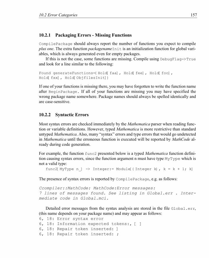
10.2 Error Categories 157
10.2.1 Packaging Errors - Missing Functions
CompilePackage should always report the number of functions you expect to compileplus one. The extra function packagenameInit is an initialization function for global vari-ables, which is always generated even for empty packages.
If this is not the case, some functions are missing. Compile using DebugFlag->Trueand look for a line similar to the following:
Found generateFunctions={Hold[faa], Hold[fee], Hold[foo], Hold[fxx], Hold[ObjfilesInit]}
If one of your functions is missing there, you may have forgotten to write the function name after BeginPackage. If all of your functions are missing you may have specified the wrong package name somewhere. Package names should always be spelled identically and are case-sensitive.
10.2.2 Syntactic Errors
Most syntax errors are checked immediately by the Mathematica parser when reading func-tion or variable definitions. However, typed Mathematica is more restrictive than standard untyped Mathematica. Also, many “syntax” errors and type errors that would go undetected in Mathematica until the erroneous function is executed will be reported by MathCode al-ready during code generation.
For example, the function func2 presented below is a typed Mathematica function defini-tion causing syntax errors, since the function argument n must have type MyType which is not a valid type:
func2[MyType n_] -> Integer:= Module[{Integer k}, k = k + 1; k] The presence of syntax errors is reported by CompilePackage, e.g. as follows:
Ccompiler::MathCode: MathCode:Error messages: 7 lines of messages found. See listing in Global.err . Inter-mediate code in Global.mci.
Detailed error messages from the syntax analysis are stored in the file Global.err,(this name depends on your package name) and may appear as follows:6, 18: Error syntax error 6, 18: Information expected tokens:, [ ] 6, 18: Repair token inserted: ] 6, 18: Repair token inserted: ;
158 10.2 Error Categories
6, 19: Error syntax error 6, 19: Information expected tokens: ; [ := 6, 22: Information restart point Note that the line number (6) and character number within the line (18) are given with respect to the file Global.mci. This intermediate file is the result of transformations of functions in packages submitted for compilation. These transformations are usually local with respect to the original code. Therefore, the meaning of these somewhat cryptic messages can easily be found by inspecting Global.mci at the indicated line number and character positions.
10.2.3 Semantic ErrorsIf there are semantic errors during code generation, e.g. type inconsistencies and references to undeclared variables or undeclared functions within a function, this will cause an error message from CompilePackage.If a function is defined as func3[Real n_] -> Integer := Module[{Integer[3] k}, k = p; k]
then the messages produced are: Ccompiler::MathCode: MathCode:Error messages: 7 lines of messages found. See listing in Global.erf. Intermediate code in Global.mci. These errors may cause Fortran90 compiler messages. 0, 0: Note In function Global`func3: 0, 0: Error Incompatible types in return statement : 0, 0: Error Assigned to "Output (return) parameter no. 1" 0, 0: Error Of type Integer 0, 0: Error Assigned from k 0, 0: Error Of type Array [ 3 ] of Integer 0, 0: Error Un-defined symbol: p
The type inconsistency occurs between the returned expression and the return type of the function. The variable p is used but it is never defined.

10.2 Error Categories 159
10.2.4 Errors During C++ Compilation and Linking
Sometimes errors occur during the compilation and linking of generated C++ code, which is performed by MakeBinary[]. These messages are presented to the user in the following form:
Ccompiler::error: Executable file is not produced due to an error.The following command returned an error: nmake @Global.cmd > Global.clog. See file Global.clog for more details.
Messages from compiler appear, for example, if the C++ compiler recognizes syntactic or semantic error in the generated code, and can be considered as internal errors of MathCode since the system should have performed more complete error checking before emitting erroneous C++ code.
Errors may also be reported from the linking phase if, for example, the user forgot to specify external libraries or object modules needed to link called external functions.
10.2.5 Internal Code Generator Errors
Occasionally internal errors in the MathCode code generator may occur, e.g., the executable om.exe crashes or stops waiting for a message. In this case you should interrupt evaluation, e.g. via the menu command Kernel/Quit Kernel (this stops all processes linked with Math-link), and inspect the files Global.cc and Global.err for error messages.
Such situations can be caused by errors in your Mathematica functions, but can be considered internal errors of MathCode since the system should have detected and reported such errors without crashing.
10.2.6 Long Compilation Times
In certain situations, using MathCode to compile Mathematica functions with very large bodies containing numerous array slice operations, e.g. on the order of many thousands of lines, may incur unacceptably long times for code generation. A temporary pragmatic fix for this problem is to divide the large function into several smaller functions and call these func-tions from the original function.

160 10.3 Appendix
10.2.7 Internal Errors During Execution of Generated Code
Occasionally internal errors occur in the generated code. This happens when, for instance, an array index in an operation is out of bounds and the MathCode array library is used with array-bounds checking turned on.
In the stand-alone mode the application issues the message to the “standard error” output unit (i.e. shown in the terminal window, like xterm in Unix or Command Prompt window in Windows) including the line number (in the MathCode library source code) where the error occurs.
In MathLink mode the "LinkConnect ... is dead" message appears.In the Unix version (both stand-alone and MathLink versions) the application also
dumps core where the call stack can be analyzed by running gdb, dbx or any other appropriate debugger.
In the Unix version (MathLink mode) a debugging tool (for example, gdb) can also be attached to the running process after it has been installed by InstallCode. By this means the code can be debugged in its dynamic behavior (note that this may require considerable computer memory and processor time resources).
In the Windows version (both stand-alone and MathLink mode), if the application is compiled with /Zi /DEBUG flags (which can easily be turned on by modifying the System/compwin.mak file), then the application suggests that the user “Start Debugger” (the complete Microsoft Visual C++ must be installed on this computer), where the call stack can be analyzed and erroneous variables can be identified. The Debugger can be started from the code in any place in your program if you call the DebugBreak() function. You may need to add #include "windows.h" in order to access it.
In the Windows version (MathLink mode), if the application is compiled with /Zi /DEBUG flags
MakeBinary[CompilerOptions->"/Zi",LinkerOptions->"/DEBUG"]It is possible to use the Tools/Debug Process option in Microsoft Visual Studio
environment. After the process is installed by InstallCode[], it can be debugged. In Globaltm.c file it is convenient to set up the break within _MLDoCallPacket() function and then follow C++ interface functions and your generated Fortran90 function step by step.
If the answer is never returned to Mathematica from a MathLink-mode call, you may suspect an infinite loop in your generated code. If disk access is heavy, you may suspect infinite recursive calls in your generated code.
When modifying and searching for the cause of an error in the generated code it is typically more convenient to use stand-alone mode. Debugging under Unix is generally easier. You should also consider command line compilation under Windows and Unix as described in Section 7.9 on page 135.
10.3 Appendix

10.3 Appendix 161
Appendix A The Compilable Mathematica Subset
This chapter of MathCode User Guide describes the MathCode C++ release 1.4.2, July 2009.
Note that the Compilable Subset varies from one release to another. Please read the Release Notes attached to your MathCode installation for the most actual information
The MathCode system provides facilities to translate a subset of the Mathematica language to compiled programs in strongly typed languages such as C++ or Fortran90. This subset includes most elementary functions and operators that compute numeric values, but ex-cludes symbolic and computer algebra-related functions that compute symbolic expressions.
However, it is possible to evaluate a symbolic expression (which may contain operations such as simplification, symbolic differentiation, substitution etc.) and generate executable numeric code from the symbolic expression resulting from this evaluation, provided that the resulting expression(s) only contain operators and functions in the compilable Mathematicasubset described here.
The arithmetic model used in the compilable Mathematica subset is specified by the IEEE Standard for Binary Floating Point Arithmetic, IEEE Standard 754.
A.1 Operations not in the Compilable SubsetThe following is a short list of those Mathematica operations and functions not in the com-pilable subset. Since the primary reason to generate compiled code is to get high perfor-mance of numeric computing code, the operations in the compilable subset are oriented to-wards efficient computing on numbers and arrays.
• Pattern matching is not supported, except for the simple case of function argument patterns like arg1_Integer or arg2_Real, which are handled by the static type system of the target language. However, overloading of functions is not supported by

162 10.3 Appendix
the current version of the code generator, e.g., there may not be two functions with the same name and arguments, one having Integer typed arguments and the other having Real typed arguments.
• When a function is declared, its arguments must be specified as single-variable names, separated with commas. As an example, node patterns like Name[a_,b_] below are not permitted.
foo [Real[2] a_, Real c_]->Real[2] := ... correct fie [Real[2] Name[a_,b_], Real c_]->Real[2]:= ... incorrect
• Arbitrary precision numbers and arithmetic are not supported. Numbers and arithmetic operations are converted to either IEEE double precision floating-point arithmetic or 32-bit (or better) integer arithmetic.
• Symbolic operations that give symbolic expressions as results are not included. However, such operations can be compiled if they are expanded to expressions in the compilable subset before code generation. Such expansion can handle many common cases of symbolic operations.
• Negative array indexing, relative to the end of arrays, is not in the compilable subset, apart from the special cases of negative constant indices, e.g., as in arr[[-3]], array ranges such as arr[[1|-n]], and submatrix extraction, as described on page 111. To index from the end of an array, FromEnd should be used with a positive argument.
• String operations are not included. except for assignment to scalar variables and argument passing.
• Input/Output operations are not included, apart from a simple Print operation.• Certain list (i.e. array) operations, specifically those that change the size of arrays or are
very inefficient, are not included in the set of functions mentioned in this appendix. Such functions can be added by the user e.g. in the system module.
• The Return[] function is not included. Therefore loop constructs like For, Whilecannot be used as expressions returning values.
• Some procedural style statements cannot be used within a CompoundExpression used in value context within arithmetic expressions. For instance, a=a+(While[i<10,i=i+1];5) cannot be translated. The expression a=a+(c=3;5), however, can be translated to C++. More details on nested constructs are given below.
• There are also a number of built-in standard Mathematica functions with numeric arguments and results which are not availiable outside Mathematica, but which can be considered to belong to the compilable subset in the sense that callback stub functions

10.3 Appendix 163
(via MathLink) for these Mathematica functions can be generated.
A.2 Predefined Functions and OperatorsExpression operators listed in this section are predefined by the code generator and will be translated correctly from Mathematica into the target language (e.g. C++ or Fortran90) with-out any additional type declarations.
Almost all operators belong to the compilable expression subset, e.g., all value-returning operators and predefined or user-defined functions without side effects (i.e. functions that do not change global variables or perform input/output).
The reason for imposing the condition of calls to side-effect free functions is that expressions can be re-ordered and common subexpressions removed in the generated code, in order to make execution more efficient. Another order in assigning and referencing global variables or performing input/output usually results in different, often unintended, program behavior. However, some restricted cases of side-effects can be re-ordered without changing the meaning of the program. One such case is when the elements of an array are assigned once, independently of each other, and are not used in the same expression. Such restricted side-effects are allowed for functions in the compilable expression subset. The code generator does not check the condition of side-effect freeness—this is the user’s responsibility.
All operators and functions in the compilable expression subset also belong to the compilable subset, which contains control expressions (If, While, For, etc.), assignment statements and functions with side effects. All real and integer constants naturally belong to the compilable expression subset, except for the special case of arbitrary-precision values. Some operators and functions can be applied to arrays or return arrays as values.
The current version of the compilable subset is oriented toward operations on real numbers and integers, and arrays containing such numbers. The basic mathematical functions usually found in C/C++ or Fortran are provided. In Mathematica there are also a number of special mathematical functions such as BesselJ[], Gamma[], etc. If the user has access to an implementation of such a function in C/C++ or Fortran, or a linkable object code library containing this function, it can be declared as an external function and thus automatically included in the compilable subset. Alternatively, such functions can be approximated by externally compiled interpolating functions or declared as callbacks,which makes the code generator produce stub functions, e.g in C/C++, that perform callback to Mathematica.
Since efficient computation based on mathematical models has been the main application of MathCode so far, the compilable Mathematica subset does not include string operations, file input, formatted file output and certain mapping and list operations.

164 10.3 Appendix
A.2.1 Statements and Value Expressions
In standard Mathematica, all predefined and user-defined functions can appear as an argu-ment of another function. Accuracy of such constructs is tested during code interpretation.
In procedural languages, such as C++ and Fortran, procedural statements cannot be used within expressions. Also, the type of allowed expressions is restricted.
In order to compile Mathematica code to procedural language, some restrictions in using statements and expressions are introduced.
In the descriptions below “stmt” means that corresponding Mathematica expressions are used as statements. In the compiled subset they do not return values, their returned values cannot be used, and they cannot be applied where values are expected. In the compiled set there is no Null value.
In descriptions below “expr” means that corresponding Mathematica expressions are used as values (l-value or r-value). These expressions must return some value when evaluated. This value cannot be Null. The word “exprs” means one or more expressions separated by a comma.
Some Mathematica constructs - Set, If, Which, CompoundExpression - can appear both as statements and as values. Some specific restrictions on their use are described below.
A.2.2 Function CallSpec syntax Operator Arg type(s) Result type(s)
funcname[exprs] ... ...
All user-defined functions which have been type declared according to the typing rules for typed Mathematica belong to the compilable subset. The same is true for functions that are declared as ExternalFunction or ExternalProcedure, and exist in a library or an ob-ject code file that can be linked together with the generated code in C++ or Fortran90. Com-pilable subset functions may only contain operations that belong to the compilable subset, or may contain non-subset operations inside bodies of functions compiled with the Evalu-ateFunction option, which will expand into compilable subset operations.
Functions with multiple return arguments can be compiled if they are type declared. Such a function can only be used on the right-hand side of an assignment statement in which the left-hand side has to be a list of variables. Thus, a call that returns multiple values can look like this:
{a, b, c} = F[x+y, 3.4];
Calls to functions with no return arguments and functions with more than one return argu-ments are to be considered statements (stmt).

10.3 Appendix 165
Calls to functions returning one argument are considered to be expressions (expr).
A.2.3 Function Definition
A function returning values can be defined as follows:
function_name[arg_type1 arg1, ..., arg_typen argn]->result_types := expr
function_name [arg_type1 arg1, ..., arg_typen argn]-> result_types := Module[variables, expr]
function_name [arg_type1 arg1, ..., arg_typen argn]-> result_types := Module[variables, stmt1;stmt2;...;expr]
A function that does not return values can be defined as follows:
function_name[arg_type1 arg1, ..., arg_typen argn]->Null := stmt
function_name[arg_type1 arg1, ..., arg_typen argn]->Null := Module[variables, stmt;]
function_name[arg_type1 arg1, ..., arg_typen argn]->Null := Module[variables, stmt1; stmt2;...;stmtn;]
Block or With can be used instead of Module.
In addition, functions can be defined as interpolating functions by using the Mathematica function FunctionInterpolation. Code generation is limited to interpolation function objects of one or two variables. Below is an example of a definition of an interpolation func-tion.
intpolmyFunc=FunctionInterpolation[myFunc[t],{t,lower,upper}];
A.2.4 Scope ConstructsSpec syntax Operator Arg type(s) Result type(s)
Module[variables,body] special none/(fnbody) Block[variables, body] special none/(fnbody) With[variables,body] special none/(fnbody)
A value can be returned from one of the above scope constructs when it occurs as a function body or when it is used in a value context within an expression. The body is restricted as

166 10.3 Appendix
follows:• If a function does not return any value, the body is a statement. If it is a
CompoundExpression statement, then all (possibly nested) elements in CompoundExpression must be statements.
In the following example two nesting levels of CompoundExpression are demonstrated:
foo[Real a_]->Null := Module[{ Real t}, (t=a+1;t=t+1);(t=t+2;t=t+3)]
• If a function returns one or more values, the body is an expression. If it is a CompoundExpression construct, then the last (possibly nested) element in the CompoundExpression must be an expression. All other components must be statements.
In the following example two nesting levels of CompoundExpression are demonstrated; note that t+4 is an expression.
foo[Real a_]->Real := Module[{ Real t}, (t=a+1;t=t+1);(t=t+2;t=t+3;t+4)]
A.2.5 Control Statements
The control statements can appear wherever a statement is allowed, in which case they do not return any value. Spec syntax Operator Arg type(s) Result type(s)s1; s2;... CompoundExpression [stmts] statements none
For [start-stmt, boolean-test-expr, incr-stmt, body-stmt] special none While [boolean-test-expr, body-stmt] special none If [boolean-test-expr, true-stmt, false-stmt] special none Which [boolean-test-expr1, stmt1 boolean-test-expr2, stmt2,...] special none Break [] - none Do [expr, iterators] special none
The CompoundExpression (a sequence of expressions separated by semicolons) Which and If can also appear as an arithmetic expression. See “Arithmetic expression” for details.

10.3 Appendix 167
A.2.6 Mapping Operations
Map expressions can be compiled in the following cases:
var=Map[f,expr]var=Map[f,expr,{n}]
The result must be directly assigned to a variable as shown. The function f can be:
• A function symbol of the compilable subset• An anonymous function, also called pure function in Mathematica• A user defined typed function for which code has been generated
n must be an integer constant. The var=Map[...] statement will be converted to a corre-sponding assignment statement with a call to Table on the right-hand side.
A.2.7 Iterator Expressions
Computing operations in Mathematica such as Do, Sum, Product and Table use iterators. Additionally there are a number of plotting functions such as Plot, ContourPlot, Den-sityPlot, Plot3D and ParametricPlot, which also use iterators but with some limita-tions in form and usually constructing sets of real values for the purpose of plotting. These plotting functions are not part of the compilable subset.
An iterator can take on one of the following forms:Form Explanation{imax} iterate imax times {i,imax} i goes from 1 to imax in steps of 1 {i,imin,imax} i goes from imin to imax in steps of 1 {i,imin,imax,di} i goes from imin to imax in steps of di {i,imin,imax},{j,jmin,jmax} Two iterators: i controls the outer iteration loop,
j controls the inner loop
Iterators in Mathematica can use either integer or real values for the iteration variables in the iteration. The compilable subset of iteration functions is limited to integer iteration vari-ables. The iteration variables in Mathematica are declared in a local scope consisting of the body (the expr below) of the iteration function. Thus, translated code in C++ needs to de-clare those iteration variables in a way that does not clash with other local variables. Typi-cally, these iteration constructs will be translated to (nested) for loops in the target lan-guage.
Iteration functions in Mathematica may or may not return a value. The functions Sum,

168 10.3 Appendix
Product, Table and Range always return a value from the iteration. Loop-terminating constructs like Return, Break, Continue, or Throw can be used inside Do. However, Doin Mathematica does not return a value except in the case of an explicit Return of a value.
The compilable subset currently does not support return of a value from a Do loop. Another constraint of the compilable subset is that the constructs Sum, Product and Tablemay currently only occur on the right-hand side of an assignment statement. Concerning Table, see also Section A.2.12.
Spec syntax Operator Arg type(s) Result type(s)Do[expr,iter1,iter2,...] special noneSum[expr,iter1,iter2,...] Real,Integer,Complex Real, Integer,ComplexProduct[expr,iter1,iter2,...] Real,Integer,Complex Real, Integer,ComplexTable[expr,iter1,iter2,...] Real,Integer,Complex Array
A.2.8 Input/Output Operations
Operator Arg type(s) Result type(s)Print[exprs] Real, Integer, Array, String,Com-
plexnone
Export[filename,expr,format]Export[filename,expr]
filename is a String ("file.fmt")expr is an Array (1D or 2D) of Real, Integer ,Complexformat is a String ("CSV" or "List")
String
var=Import[filename,format]var=Import[filename]
filename is a String ("file.fmt")format is a String ("CSV" or "List")
Array (1D or 2D) of Real Integer or Complex
(Export and Import are new in MathCode 1.4)
When Print[] is performed the output is placed on the standard output stream of the external process where the generated code is executing. For some operating environments (e.g. with MathLink) this stream is not available.
In Export[] and Import[] the format is determined by the argument format which can be "CSV" or "List". If it is missing, then the format is determined by the suffix of the filename (".CSV" or ".csv")
The Import[] can be used within the assignment statement only. If this is the last
10.3 Appendix 169
statement of the function, it is recommended to write foo[]:=(var=Import[...];var). The type of variable var should match the type of the values saved in the file.
In contrast to Mathematica behavior, if var is a 2D array, but the file contains just 1D data, the 1-column 2D array is created (such as {{1},{2},{3}}.
Only rectangular 2D arrays are supported. If var has a Complex base type, then Complex, Real and Integer data are accepted for Import operation.
No other Export/Import formats are supported, and no format-specific options are supported.
Import of Complex numbers ("CSV" or "List") is not really supported in Mathematica. It requires conversion of strings to expressions (ToExpression[]); this is not needed for MathCode.
The recommended ways to perform other formatted input/output from generated code are via callback functions or external functions.
A.2.9 Standard Arithmetic and Logic Expressions
Spec syntax Operator Arg type(s) Result type(s)== Equal[e1,e2] Real,Integer,Array,
ComplexBoolean
!= Unequal[e1,e2] Real,Integer,Array, Complex
Boolean
> Greater[e1,e2] Real, Integer, Complex Boolean< Less[e1,e2] Real, Integer, Complex Boolean>= GreaterEqual[e1,e2] Real, Integer, Complex Boolean<= LessEqual[e1,e2] Real, Integer, Complex Boolean
Inequality[exprs...] special Boolean! Not[e] Boolean Boolean|| Or[exprs...] Boolean Boolean&& And[exprs...] Boolean Boolean+ Plus[exprs...] Real,Integer,Array,
ComplexReal,Integer,Array, Complex
- Subtract[e1,e2] Real,Integer,Array, Complex
Real,Integer,Array, Complex
- Minus[exprs...] Real,Integer,Array, Complex
Real,Integer,Array, Complex

170 10.3 Appendix
* Times[e1,e2] Real,Integer,Array, Complex
Real,Integer,Array, Complex
/ Divide[e1,e2] Real,Integer,Array, Complex
Real, Array, Complex
Mod[e1,e2] Real,Integer,Array, Complex
Real, Array, Complex
Rational[e1,e2] Real,Integer Real^ Power[e1,e2] Real,Integer,Array,
ComplexReal,Integer,Array, Complex
Abs[e] Real,Integer,Array, Complex
Real,Integer,Array, Complex
If[boolean-test-expr,true-expr,false-expr]
1st arg Boolean;Real,Integer,Array, Complex
Real,Integer,Array, Complex
Sign[e] Real,Integer,Complex Integer,ComplexFloor[e] Real,Array, Complex Integer,ComplexCeiling[e] Real,Array, Complex Integer,ComplexRounde[e] Real,Array, Complex Integer,ComplexSqrt[e] Real,Integer,Array,
ComplexReal, Array, Complex
Exp[e] Real,Integer,Array, Complex
Real, Array, Complex
Log[e] Real,Integer,Array, Complex
Real, Array, Complex
Sin[e] Real,Integer,Array, Complex
Real, Array, Complex
Cos[e] Real,Integer,Array, Complex
Real, Array, Complex
Tan[e] Real,Integer,Array, Complex
Real, Array, Complex
Cot[e] Real,Integer,Array, Complex
Real, Array, Complex
Sec[e] Real,Integer,Array, Complex
Real, Array, Complex
Spec syntax Operator Arg type(s) Result type(s)

10.3 Appendix 171
Csc[e] Real,Integer,Array, Complex
Real, Array, Complex
ArcSin[e] Real,Integer,Array, Complex
Real, Array, Complex
ArcCos[e] Real,Integer,Array, Complex
Real, Array, Complex
ArcTan[e] Real,Integer,Array, Complex
Real, Array, Complex
ArcTan[e1,e2] Real,Integer,Array, Complex
Real, Array, Complex
ArcSinh[e] Real,Integer,Array, Complex
Real, Array, Complex
ArcCosh[e] Real,Integer,Array, Complex
Real, Array, Complex
ArcTanh[e] Real,Integer,Array, Complex
Real, Array, Complex
ArcCoth[e] Real,Integer,Array, Complex
Real, Array, Complex
IntegerPart[e] Real,Integer,Array, Complex
Integer, Array, Complex
FractionalPart[e] Real,Integer,Array, Complex
Real,Integer,Array, Complex
Quotient[e1,e2] Real,Integer,Array Integer,ArrayMax[m,n] Real,Integer Real,IntegerMin[m,n] Real,Integer Real,IntegerMax[e] Array of Real RealMax[e] Array of Integer IntegerMin[e] Array of Real RealMin[e] Array of Integer IntegerOuter[e1,e2] 1D-Array,1D-Array ArrayCross[e1,e2,...,en] Arrays ArrayTranspose[e] 2D-Array 2D-Array
e1 . e2 ... Dot[e1,e2,...] Array Real,Integer,Array
Spec syntax Operator Arg type(s) Result type(s)
172 10.3 Appendix
For functions with two arguments, the following rule applies: one argument can be Array and another argument can be either scalar (of the same type as the base type of the array) or Array of the same dimension. This does not apply to == and !=.
Those functions that return an integer value converted from real: Sign, Floor,Ceiling and Round, give an undefined value or an exception (depending on the underlying target language, e.g. C++) when trying to fit too large a number into an integer.
The following functions are implemented according to Mathematica semantics1:
• IntegerPart returns (int)x for Reals and int(Re(x)+ i int(Im(x)) for Complexes
• FractionalPart returns x-IntegerPart(x)
• Quotient[m,n] returns Floor(m/n) for Reals. It is not defined for Complexes
• Floor(x) for Complexes is Floor (Re(x) + i Floor(Im(x) ) ) • Mod[m,n] returns m%n if m and n have the same sign and m%n+n if they have opposite
signs. If m or n is a Real then m-n*floor(m/n) is returned. If there is a Complexargument passed to these functions they return a Complex result
• The Rational function is part of the compilable subset. It is treated exactly like Divide and converted to Divide during code generation.
• The special purpose Cross function computes the cross product of n-1 vectors of length n and returns a vector of length n. For example, Cross[{2,3,4},{5,6,7}] returns the vector {-3,6,-3} which is orthogonal to the two argument vectors. The function Cross is implemented for n= 3, 4, 5 according to the generalized Mathematicadefinition.
The CompoundExpression construct when used as a value within another statement or expression (but not as a function definition) has the following limitation: the statements (stmt1,..., stmtn) allowed within CompoundExpression are assignments (Set), Print or Put only.2 Assignment to list cannot be used there. For instance:
CompoundExpres-sion[ stmt1, ...,stmtn ,expr]
statements expr
1. Read Release Notes for more information 2. Read Release Notes for more information
Spec syntax Operator Arg type(s) Result type(s)
10.3 Appendix 173
a=b+(While[i<10,i=i+1] ; c); (* not allowed *)
a=Foo[{d,f}={3,5} ; c ]; (* not allowed *)
a=b+(Print[x];c); (* allowed *)
foo[Real a_]->Real=(i=i-1;(While[i<10,i=i+1] ; c)) // allowed
A.2.10 Named ConstantsSpec syntax Operator Arg type(s) Result type(s)
True - Boolean False - Boolean E - Real Pi - RealI - Complex
Variables of type Boolean are not supported in the compilable subset. If boolean values are assigned to integer variables, False becomes 0, True becomes non-zero. Named constants are expressions (expr).
A.2.11 Assignment ExpressionsSpec syntax Operator Arg type(s) Result type(s)var := e SetDelayed[var,e] all types value var = expr Set[var,expr] all types value {vars} = funcall Set[List[vars],funcall] - none {vars} = expr Set[List[vars],expr] - none
The supported main assignment functions, Set and SetDelayed, have return types. There-fore these can be used both as statements and as expressions.
The arguments (left- and right-hand side of the assignment) must be of compatible types. Left- and right-hand side arguments are compatible if they can be made into the same
type by performing standard type promotion (e.g. promoting integer to real, or a scalar or lower-dimensional array to a higher-dimensional array), provided that this promotion does not change the type of the left-hand side. If it does, then the assignment is illegal. This means that an expression of a real type cannot be assigned to a variable of integer type without using explicit conversion of the right-hand side (e.g. using Floor[]).
In the case of simultaneous assignment to a list of variables {vars}, funcall must be a call to a function returning a list of the same length as the list on the left-hand side of the assignment. Also, the vars list on the left-hand side may only contain variables.

174 10.3 Appendix
A.2.12 Array Data ConstructorsSpec syntax Operator Arg type(s) Result type(s)
Array[exprfunc,{dim1,dim2,...}] exprfunc constant Array Table[expr,{dim1},{dim2},...] Array Table[expr,{i,imin,imax,istep},{j,jmin,jmax,jstep},...] Array IdentityMatrix[n] Integer Array (2D) DiagonalMatrix[vec] Array (1D) Array (2D) Range[n] Real or Integer Array (1D) Range[start, end] Real or Integer Array (1D) Range[start, end, step] Real or Integer Array (1D)
See also section A.2.7 concerning iterator expressions. The following limitations currently apply to compilation of Array, Table, IdentityMatrix and DiagonalMatrix calls: the exprfunc used by Array may only be a constant function; local iteration variables used in iterators to Table are automatically created but are always of type Integer; calls to Array, Table, IdentityMatrix and DiagonalMatrix may only occur on the right- hand side of an assignment statement, for example:
arrvariable = Table[3.1+i+j, {i,5}, {j,1,10,2}]
A.2.13 Array Data Manipulation
(new in MathCode 1.4)Operator Arg type(s) Result type(s)
Append[ar2,ar1] The rank of ar2 is one Same as ar2 higher than the rank of ar1 ar1 is Real, Integer, Complex, or 1D,2D,3D array of them
Prepend[ar2,ar1] same as Append[]
Drop[ar,idx] ar is Real, Integer, Same as ar Complex, or array of them; idx is Integer
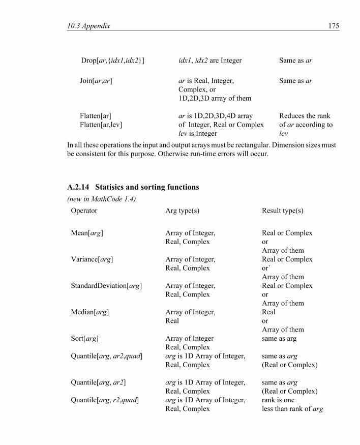
10.3 Appendix 175
Drop[ar,{idx1,idx2}] idx1, idx2 are Integer Same as ar
Join[ar,ar] ar is Real, Integer, Same as ar Complex, or 1D,2D,3D array of them
Flatten[ar] ar is 1D,2D,3D,4D array Reduces the rank Flatten[ar,lev] of Integer, Real or Complex of ar according to
lev is Integer levIn all these operations the input and output arrays must be rectangular. Dimension sizes must be consistent for this purpose. Otherwise run-time errors will occur.
A.2.14 Statisics and sorting functions(new in MathCode 1.4)
Operator Arg type(s) Result type(s)
Mean[arg] Array of Integer, Real or Complex Real, Complex or
Array of them Variance[arg] Array of Integer, Real or Complex
Real, Complex or´ Array of them
StandardDeviation[arg] Array of Integer, Real or Complex Real, Complex or
Array of them Median[arg] Array of Integer, Real
Real or Array of them
Sort[arg] Array of Integer same as arg Real, Complex
Quantile[arg, ar2,quad] arg is 1D Array of Integer, same as arg Real, Complex (Real or Complex)
Quantile[arg, ar2] arg is 1D Array of Integer, same as arg
Real, Complex (Real or Complex) Quantile[arg, r2,quad] arg is 1D Array of Integer, rank is one
Real, Complex less than rank of arg

176 10.3 Appendix
(Real or Complex) Quantile[arg, r2] arg is 1D Array of Integer, rank is one
Real, Complex less than rank of arg (Real or Complex)
All statistics functions (except Quantile) operate on rectangular numerical 1D, 2D, 3D and 4D arrays with Integer, Real and Complex base types. Arrays with Real and Complex types are returned.The command Median[] does not work with Complex numbers in Mathematica.The operations Mean[], Variance[], StandardDeviation[] and Median[] reduce the rank of array by one; e.g. if an array of type Real[2,3,4] is given as an argument, then Real[3,4] is returned.In the case of Quantile[] certain rules apply. The argument arg should be a 1D array of Integer , Real or Complex. The argument ar2 should be 1D array of Reals. The argument r2 should be a Real. The argument quad is a quadruple {{Real,Real}, {Real,Real}}. If ar2 is used, the command performs the same rank reduction as in above commands. If r2 is used then the result has the same type as arg. The base type of the result is propagated from Integer to Real, i.e. Integers are never retuned from this function.
A.2.15 Array Dimension FunctionsSpec syntax Operator Arg type(s) Result type(s)
Dimensions[arr][[i]] Array Integer Dimensions[arr] Array Array of Integers Length[arr] Array Integer
A.2.16 Array IndexingSpec syntax Operator Arg type(s) Result type(s)arr[[ind]] Part[arr,ind] Integer Integer,Real,Array
Extract[a1,a2] Array of Integer constants Array of Element Type
Extract[a,i] takes an array of rank 1,2,3, or 4 as the first argument and a vector of inte-gers as the second argument. It returns the base element of the first array. If the size of the vector i is not equal to the rank of a then a runtime error may occur.
The Part construct can be used in both the left and right parts of an assignment. The number of indices should be less than or equal to the rank of the array. For instance, these operations are allowed:

10.3 Appendix 177
Declare[Real[3,3,3,3] a4;Real[3,3,3] a3;Real[3,3] a2;Real[3] a1;Real x;...
]
a3[1]=a2; a3[2,1]=a1; a3[3,1,2]=5.5;a2[1]=a1; a2[2,2]=7.7;a4[2,3,1,2] = 6.6;
x=Extract[a4,{2,3,1,2}]
a4[1,2,3]=a1;a4[1,2]=a2;a4[1]=a3;
This operation is not permitted:
a1=Extract[a4,{2,3,1}] (* Wrong rank. May cause run time error *)
A.2.17 Array Section OperationsSpec syntax Operator Arg type(s) Result type(s)arr[[_]] Part[arr,...] special Array arr[[n1|_]] Part[arr,...] special Array arr[[n1|n2]] Part[arr,...] special Array
These are extensions to standard Mathematica. See Chapter 3 for more information. These operations are currently supported for up to four dimensions by the code generator and for arbitrary dimensions within Mathematica and can be used on both the left- and right-handsides of assignment statements.
A.2.18 Other ExpressionsSpec syntax Operator Arg type(s) Result type(s){e1, e2,...} List[expressions] all types Array
Apply[f, args]

178 10.3 Appendix
List
List is partially implemented when appearing within expressions, for instance when used as an actual parameter to a function. The arguments of List can be:
• Real expressions (creates an Array of Real)• Integer expressions (creates an Array of Integer)• Arrays of Real (creates a 2-, 3-, 4-dimensional Array of Real). Can be nested.• Arrays of Integer (creates a 2-, 3-, 4-dimensional Array of Integer). Can be nested.
List is also implemented when it appears on the left-hand side of an assignment. In this case Part is applied to the right-hand side, and all types should match1:
{a,b,{c,d}}=x (* is the same as a=x[[1]];b=x[[2]];c=x[[3,1]];d=x[[3,2]]; *)
A runtime error may occur if a matrix appears to be non-rectangular.These special cases are implemented:
variable={expr1,...,exprn}
{var1,...,varn}=expression
{var1,...,varn}={expr1,...,exprn}
Apply
The following cases of Apply are implemented:
• Plus, Power and Times applied to an expression with assignment to a typed variable:
var=Apply[Plus,expression] var = Plus @@ expression var=Apply[Power,expression] var = Power @@ expression var=Apply[Times,expression] var = Times @@ expression
• Apply of typed functions, for example
var=Apply[function,expression] function @@ expression
The number of arguments to the function must match the length of the expression.
1. Read Release Notes for more information

10.3 Appendix 179
• Apply of anonymous (pure) functions, for example
var=Apply[Sin[#1+#2]&,expression] Sin[#1+#2]& @@ expression
The code Apply[foo,expr], equivalent to foo @@ expr, will be converted to foo[expr[[1]],expr[[2]],...]. Therefore the behavior will be different from that of Mathematica (and hence probably unexpected) if the number of parameters is not the same as the length of the expression expr.
It is the user’s responsibility to ensure that the number of arguments to the pure function is the same as the length of the expression. The number of arguments is taken as the maximum slot number (for Function[body]) or the length of the variable list (for Function[{vars...}, body]).
The expression given to Apply may be computed many times which may be a performance issue. If the expression is large, it is better to assign the expression to a temporary variable before using Apply.
No level specification is supported for Apply.
A.2.19 Operators Which May Have Side-effectsSpec syntax Operator Arg type(s) Result type(s)var := e SetDelayed[var,e] all types none var = expr Set[var,expr] all types none {vars}=funcall Set[List[vars],funcall] special none
For[start,test,incr,body] special none While[test,body] special none Do[expr,{iter1...},{iter2...}..] special none If[test,true-expr,false-expr] special none/expr If[test,true-expr] special none/expr Which[test1,val1,test2,val2,...] special none Break[] - none
e1; e2; .. CompoundExpression[exprs] special type of last expression Module[variables,body] special none/function value Block[variables, body] special none/function value With[variables,body] special none/function value
A.3 Predefined TypesAs already mentioned, there are a number of predefined basic types included in the com-pilable subset of Mathematica. There is also a set of predefined types, primarily array types, which are included for convenience.
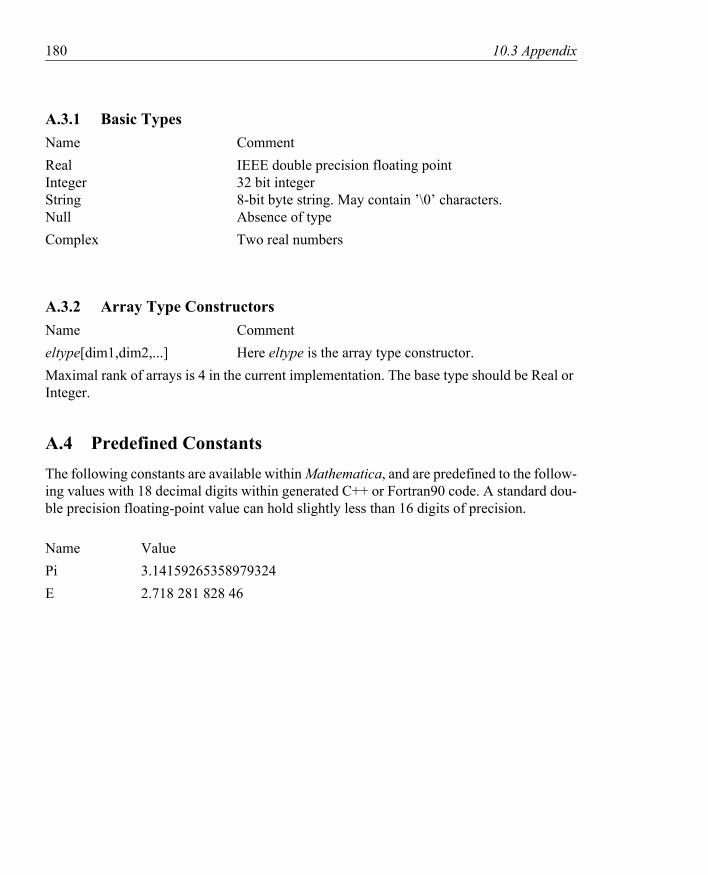
180 10.3 Appendix
A.3.1 Basic TypesName CommentReal IEEE double precision floating point Integer 32 bit integer String 8-bit byte string. May contain ’\0’ characters. Null Absence of typeComplex Two real numbers
A.3.2 Array Type ConstructorsName Commenteltype[dim1,dim2,...] Here eltype is the array type constructor.Maximal rank of arrays is 4 in the current implementation. The base type should be Real or Integer.
A.4 Predefined ConstantsThe following constants are available within Mathematica, and are predefined to the follow-ing values with 18 decimal digits within generated C++ or Fortran90 code. A standard dou-ble precision floating-point value can hold slightly less than 16 digits of precision.
Name ValuePi 3.14159265358979324E 2.718 281 828 46
181
Symbols# (Slot for pure function) 179$Context 150$MathCodeMakeFile 124$MCRoot 53& (pure function) 179. 171: 74= (Set) 173, 179> 169@@ (Apply) 178 176_ 74, 177{ } 177| 74, 177
AAbs 170ActivateCode 130, 131allocation
without initialization 105Append 174Apply 178argument passing
by reference 138array 112, 174
allocation 103initialization 103runtime sized 105slice operations 73type constructor 94
array indiceslower bounds 109negative indices 111upper bounds 110
assignment expressions 173
Bbasic types 91BLAS 137Block 165, 179Break 166, 179BuildCode 130
CC 140, 142C++ 140call by value 138CallBackFunctions 121, 133callbacks
stub functions 134CCOPT 124Ceiling 172CleanMathCodeFiles 71code generation
preceded by symbolic evaluation 39
standard 38column matrix 77column vectors 76Command Shell 136compilable expression subset 163compilable subset 161CompilePackage 118, 151Compiler 123CompilerOptions 124compile-time constants 93CompoundExpression 166, 172, 179Constant 93Constant Declarations 93constants
compile-time 93named 93, 173
182
constructorarray types 94data 95type 94
control statements 166
Ddata constructor 95data flow 138DeactivateCode 130, 131DebugFlag 123declaration of several variables 92declarations 85
constant 93functions 87, 96multiple variables 92separate 92, 98variable 92
Declare 23, 92, 93, 96, 98declared separately 92Depth 113DiagonalMatrix 106, 112, 174dimension size placeholders 107Dimensions 176DisabledMathLinkFunctions 121Divide 170, 172Do 166, 168, 179Dot 171DownValues 131, 132Drop 174, 175dual type system 22
EE 173Equal 169
error categories 156errors
categories 156semantic 158syntax 157
EvaluateFunctions 120execution parameters 103Export 168expressions
assignment 173external
function value 139functions 137object code 150programs 133variables 137
ExternalCall 132ExternalDownValues 131, 132ExternalFunction 139ExternalLanguage 121, 140ExternalProcedure 139Extract 176
FFalse 173Flatten 175Floor 172For 166, 179Fortran 140, 142, 143Fortran77 147FractionalPart 172function
declaration 87functions 96
external 137multiple return values 97

183
no input parameters 96no return value 97predefined 163
GGaussSolveForLoops 56GaussSolveMatlab 54Global 20, 118global variables 102Greater 169GreaterEqual 169
IIdentityMatrix 106, 112, 174IEEE Standard 754 161If 166, 170, 179Import 168IMSL 137index range notation 74Inequality 169InlineFlag 122Input/Output 162Install 131InstallCode 50, 131Integer 180IntegerPart 172integration 130
compiled code 117external code 118
intermediate form 116iterator expressions 167
JJoin 175
LLanguage 123Length 113, 176Less 169linker 136LinkerOptions 124LINKOPT 124, 129LinPack 137List 178list structures 94Listable 104lists as arrays 94local variables 103
MMacroRules 122main() 121MainFileAndFunction 121MakeBinaries 122MakeBinary 50, 128, 151Map 167MathCode 17MathCodeConfig.m 123Mathematica graphics 133MathLink 18, 21, 116, 120, 128, 130MatrixQ 113Max 171Mean 175Median 175Mod 172Module 165, 179mprep 116
NNamed 93
184
NeedsExternalLibrary 121, 129, 150NeedsExternalObjectModule 121,
122, 129, 150Null 91, 180
OOpenGL 137operators
predefined 163OuterProduct 171overloading 161
Ppackages
system 135parameter passing
reference 144value 145
Part 73, 176, 177partial evaluation 127pattern matching 161patterns 87performance
SinSurface 51Pi 173Plus 169Prepend 174Print 168Product 168Protected 93
QQuantile 175, 176Quotient 171, 172
RRange 112, 174RangeCheckFlag 122Rational 170, 172Real 91, 180reference parameters 144, 145Return 162Round 172row matrix 76row vectors 76
Sscope constructs 165semantic errors 158separately 98Set 173, 179SetCompilationOptions 119, 150, 151SetDelayed 173, 179Sign 170, 172single-assignment 109SinSurface 41Sort 175SourceDownValues 131, 132StandAloneExecutable 129, 136StandardDeviation 175static typing 85String 180stub function 131subexpression elimination 126Sum 168syntax errors 157system package 135
TTable 112, 174

185
target code type 116TensorRank 113True 173type 22
basic 91constructor 94static 85
UUnCompiledFunctions 120UninstallCode 71, 131
Vvalue parameters 145variables
declaration 92external 137global 102local 103
Variance 175Vector 73VectorQ 113Vectors 76vectors
column 76one dimensional 76row 76
WWhich 166, 179While 166, 179With 165, 179

186

187

188

189

190


