ORI GIN AL PA PER

PGA distributions and seismic hazard evaluationsin three cities in Taiwan

Jui-Pin Wang • Su-Chin Chang • Yih-Min Wu • Yun Xu

Received: 20 October 2011 / Accepted: 11 July 2012 / Published online: 3 August 2012� Springer Science+Business Media B.V. 2012

Abstract This study first presents the series of peak ground acceleration (PGA) in the

three major cities in Taiwan. The PGAs are back-calculated from an earthquake catalog

with the use of ground motion models. The maximums of the 84th percentile (mean ? one

standard deviation) PGA since 1900 are 1.03, 0.36, and 0.10 g, in Taipei, Taichung, and

Kaohsiung, respectively. Statistical goodness-of-fit testing shows that the series of PGA

follow a double-lognormal distribution. Using the verified probability distribution, a

probabilistic analysis was developed in this paper, and used to evaluate probability-based

seismic hazard. Accordingly, given a PGA equal to 0.5 g, the annual exceedance proba-

bilities are 0.56, 0.46, and 0.23 % in Taipei, Taichung, and Kaohsiung, respectively; for

PGA equal to 1.0 g, the probabilities become 0.18, 0.14, and 0.09 %. As a result, this

analysis indicates the city in South Taiwan is associated with relatively lower seismic

hazard, compared with those in Central and North Taiwan.

Keywords Probability-based seismic hazard � Double-lognormal distribution � Three

major cities in Taiwan

Electronic supplementary material The online version of this article (doi:10.1007/s11069-012-0298-y)contains supplementary material, which is available to authorized users.

J.-P. Wang (&) � Y. XuDepartment of Civil and Environmental Engineering, The Hong Kong University of Science andTechnology, Kowloon, Hong Konge-mail: jpwang@ust.hk

S.-C. ChangDepartment of Earth Sciences, The University of Hong Kong, Pokfulam, Hong Kong

Y.-M. WuDepartment of Geosciences, National Taiwan University, Taipei, Taiwan

123

Nat Hazards (2012) 64:1373–1390DOI 10.1007/s11069-012-0298-y

1 Introduction

Taiwan is located in the western portion of the circum-Pacific seismic belt, and the area is one

of the most seismically active regions in the world. Thus, the Taiwan Island has a high rate of

crustal deformation, and has been repeatedly struck by catastrophic earthquakes. The Chi-Chi

earthquake in 1999 was the recent catastrophic event that caused thousands of casualties and

countless loss in economy. Local researchers have spent lots of efforts on a variety of

earthquake-related studies, in a hope to develop local earthquake-resistant designs, and to

mitigate potential earthquake hazards in Taiwan. The Central Geological Survey, Taiwan,

has launched the investigation into active faults on the island, and the results have been

published with periodical updates (Lin et al. 2008, 2009). Other studies, including the

probabilistic seismic hazard analysis (PSHA) (Cheng et al. 2007) and earthquake early

warning (Wu and Kanamori 2005a, b), have also been conducted for the region of Taiwan.

Earthquakes are believed to be unpredictable, or the predictions of the exact time,

location, and size of next catastrophic earthquakes are impossible (Geller et al. 1997).

However, the community agrees that seismic hazard analysis is a logical and practical

approach (Geller et al. 1997), and can be used for developing the earthquake-resistant

designs of engineered structures. PSHA, developed in the late 1960s (Cornell 1968), is one

of the methods with a few case studies being performed for some regions in the past decade

(e.g., Cheng et al. 2007; Sokolov et al. 2009). Its growing popularity is also reflected by the

fact that a couple technical guidelines have used it for developing the earthquake-resistant

designs of critical structures (U.S. NRC 2007; IAEA 2002). Although PSHA has become

the standard procedure in a site-specific design, the legitimacy in its framework has been

under debate (Krinitzsky 1993a, b; Bommer 2002, 2003; Castanos and Lomnitz 2002). On

the other hand, a few other probability-based approaches have been also developed for

evaluating earthquake potentials (Jafari 2010; Wang et al. 2011).

This study aims to evaluate the seismic hazard in Taiwan by a new probabilistic pro-

cedure statistically analyzing the distribution of peak ground motions (PGA) in the past

110 years. The seismic hazards in three major cities in the North (Taipei), Central (Tai-

chung), and South (Kaohsiung) Taiwan are evaluated by the approach, through a reliable

earthquake catalog since 1900 and local ground motion models reported in the literature.

2 Distributions of semi-observed ground motion

2.1 Semi-observed ground motion

During an earthquake, the ground motion at a site can be measured by modern instru-

mentation. But unlike an earthquake catalog, there is yet a ground motion catalog available

for a given location. Since earthquake-induced ground motion at the site of interest can be

estimated by an attenuation relationship, a series of site-specific ground motions can be

established from an earthquake catalog along with suitable ground motion models. Since

they are not directly measured or observed, we consider them the semi-observed ground

motions in this study.

2.2 Ground motion models

A ground motion model provides a predictive relationship between an earthquake and its

ground motion at a site (Kramer 1996). Its general expression is as follows:

1374 Nat Hazards (2012) 64:1373–1390

123

ln Y ¼ f ðh1; . . .; hnÞ ¼ f ðXÞ; 4rln Y ¼ r� ð1Þ

where Y denotes ground motion; h1; . . .; hn denote earthquake variables, for example,

magnitude, distance; X denotes the set of earthquake variables h1; . . .; hn; f denotes a

predictive function. The model uncertainty rln Yð Þ is prescribed by a constant r� during its

development. It is worth noting that the logarithm of ground motion (ln Y) follows a

normal distribution, with its mean lln Yð Þ and standard deviation rln Yð Þ equal to f Xð Þ and

r�, respectively (Kramer 1996). As a result, the relationship between Z (standard normal

variate), Y, f Xð Þ, and r� is as follows (Ang and Tang 2007):

Z ¼ ln Y � lln Y

rln Y

) ln Y ¼ Z � rln Y þ lln Y

) ln Y ¼ Z � r� þ f Xð Þ) Y ¼ exp Z � r� þ f Xð Þð Þ

ð2Þ

Since ln Y follows a normal distribution, its 50th and 84th percentiles are corresponding

to Z equal to 0 and 1, respectively. With 0 and 1 being substituted into Eq. 2, the 50th and

84th percentiles of Y for a given f Xð Þ and r� become:

Y50 ¼ exp f Xð Þð Þ ð3Þ

Y84 ¼ exp r� þ f Xð Þð Þ ð4Þ

2.3 Magnitude and distance thresholds

Similar to PSHA, magnitude and distance thresholds are the two parameters associated

with the following analytical procedure. The earthquakes with a small magnitude or large

source-to-site distance are unlikely to cause structural damage, and those will be not

considered in seismic hazard assessments. In this study, a ‘‘featured’’ earthquake is defined

as one with large magnitude and small source-to-site distance, potentially resulting in a

destructive ground motion at a site of interest. In the following analyses, six sets of

magnitude and distance thresholds (M0, R0) were used, which are (5.5 Mw, 100 km),

(5.5 Mw, 150 km), (5.5 Mw, 200 km), (6.0 Mw, 150 km), (6.0 Mw, 200 km), and (6.5 Mw,

250 km). It should be noted that the thresholds are in accord with the evaluation of

earthquake potentials in the city of Tehran, Iran (Jafari 2010).

2.4 Inputs: earthquake catalog, ground motion model, etc

The earthquake catalog used in analyzing the distribution of annual maximum earthquake

magnitudes around Taiwan (Wang et al. 2011) was adopted in this study. Figure 1 shows

the spatial distribution of more than 50,000 earthquakes since 1900. The catalog was

declustered, and the earthquakes were recorded in local magnitude ML. The ground motion

models used in the recent PSHA studies for Taiwan were also used (Cheng et al. 2007).

Table 1 summarizes the four ground motion models for PGA estimation, and each of them

was used with an equal weight to consider the (epistemic) uncertainty. Because the

magnitudes in ground motion models and the earthquake catalog are different, an empirical

relationship is needed for the conversion between moment magnitude Mw and local

magnitude ML as follows (Wu et al. 2001):

Nat Hazards (2012) 64:1373–1390 1375

123

ML ¼ 4:533� lnðMwÞ � 2:091 ð5Þ

2.5 The 50th PGA in the three major cities in Taiwan

As an example, Fig. 2 shows the distributions of the 50th PGAs near Taipei, calculated

from the 128 featured earthquakes given the threshold equal to (6.0 Mw, 200 km). The

mean, coefficient of variation (COV), and maximum of the 50th PGA are 22.4 gal, 235 %,

and 579 gal, respectively. The maximum is associated with the earthquake in 1909 with its

magnitude and source-to-site distance of 7.9 Mw and 5.5 km, respectively.

Figure 3 shows the statistics of the 50th PGAs near the three cities under the six

thresholds. It was found that the mean and COV show a negative correlation. In contrast, a

positive correlation was observed between earthquake rate and COV. The possible cause

for the positive correlation observed is suggested as follows. That is, the higher likelihood

of extreme occurrences is expected given more events. With an extreme PGA, the variation

of back-calculated PGA will increase significantly. On the other hand, the negative cor-

relation between PGA’s mean and COV is expected owing to the definition of COV beingstandard deviation=mean.

In addition, the numbers of featured earthquakes and the mean values of the 50th PGA

in Taipei and Taichung are found comparable, and both are higher than those of Ka-

ohsiung. The higher rate in Taipei and Taichung results from their location being closer to

the subduction zone located in the eastern offshore, where a high concentration of earth-

quakes is observed in Fig. 1. In contrast, the city in the south is subject to a relatively lower

earthquake threat in terms of earthquake frequency. It was also found that except for

Kaohsiung, the maximum PGA is independent of the six thresholds. With the threshold

(6.0 Mw, 250 km) being used in Kaohsiung, the maximum is 53 gal associated with

120 121 122 123

22

23

24

25

120 121 122 123

22

23

24

25

Kaohsiung

Taichung

Taipei

Lat

itu

de

(°N

)

Longitude (°E)

Fig. 1 Spatial distribution of theseismicity around Taiwan since1900 (Wang et al. 2011)

1376 Nat Hazards (2012) 64:1373–1390

123

magnitude and distance of 9.3 Mw and 228 km, respectively. For others, the maximum

becomes 51 gal associated with magnitude and distance of 7.4 Mw and 75 km,

respectively.

120 121 122 123

22

23

24

25

26 solid circle => events less than 200 km near Taipei

Kaohsiung

Taichung

(a) Spatial distribution

Taipei

Latit

ude

(0 N)

Longitude (0E)

0 20 40 60 80 100 120 140

0

100

200

300

400

500

600

Sample Size = 128Mean = 22.4 galCOV = 235 %Maximum = 579 gal

(b) Temporal distribution

gal

The sequence of 50th PGA

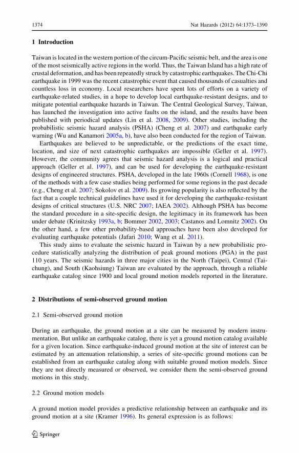
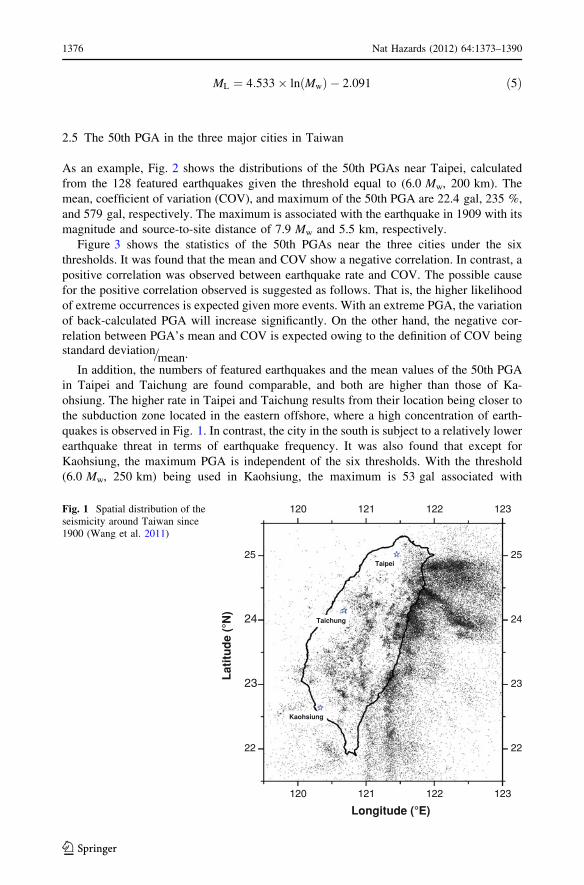
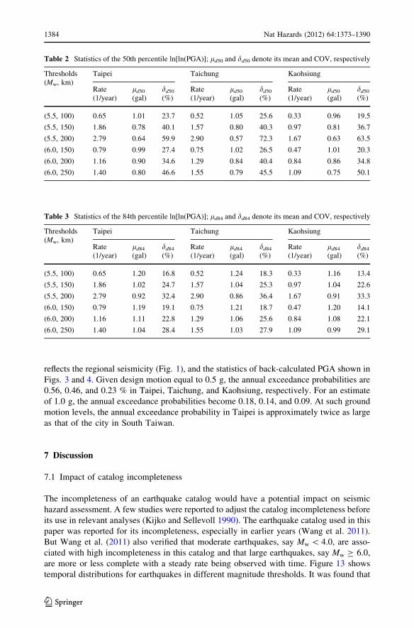
Fig. 2 128 back-calculatedPGAs near Taipei since 1900with the threshold of (6.0 Mw,200 km): a spatial distributionand b the magnitudes of groundmotions

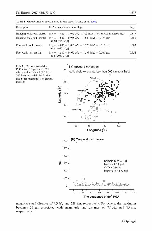
Table 1 Ground motion models used in this study (Cheng et al. 2007)

Description PGA attenuation relationship rlny

Hanging wall, rock, crustal ln y = -3.25 ? 1.075 Mw-1.723 ln[R ? 0.156 exp (0.62391 Mw)] 0.577

Hanging wall, soil, crustal ln y = -2.80 ? 0.955 Mw - 1.583 ln[R ? 0.176 exp(0.603285 Mw)]

0.555

Foot wall, rock, crustal ln y = -3.05 ? 1.085 Mw - 1.773 ln[R ? 0.216 exp(0.611957 Mw)]

0.583

Foot wall, soil, crustal ln y = -2.85 ? 0.975 Mw - 1.593 ln[R ? 0.206 exp(0.612053 Mw)]

0.554

Nat Hazards (2012) 64:1373–1390 1377

123

2.6 The 84th PGA in the three major cities in Taiwan

The results shown in Fig. 3 are associated with the 50th PGA without considering the (ale-

atory) uncertainty r� of ground motion models. Using Eq. 4, Fig. 4 shows the statistics of the

84th PGA for the three cities. The means and maximums are increased due to the ‘‘plus one

r�,’’ with an approximately 70 % increase in mean and maximum being observed. However,

the COVs of the 84th PGA remain a comparable level as the 50th percentile.

3 Probability distribution

3.1 Variable transformation

In Fig. 2b, the distribution of the 50th PGAs is highly asymmetrical. The widely used

normal distribution is judged to be improper in modeling such an asymmetrical variable. In

order to find a suitable probability model, other asymmetrical models, such as lognormal

distribution, can be tested in a trial-and-error basis, or using variable transformation.

Figure 5 shows that the series of (single-) logarithm and double-logarithm of PGAs in

Fig. 2b demonstrating an increased level of symmetry in the transformed variables,

especially for ln[ln(PGA)]. In other words, the normal distribution could become suitable

in modeling the transformed variables.

(5.5, 100) (5.5, 150) (5.5, 200) (6, 150) (6, 200) (6, 250)0

100

200

300

(5.5, 100) (5.5, 150) (5.5, 200) (6, 150) (6, 200) (6, 250)

10

15

20

25

30

(5.5, 100) (5.5, 150) (5.5, 200) (6, 150) (6, 200) (6, 250)

50

100

150

200

250

Num

ber

of E

arth

quak

es Taipei Taichung Kaohsiung

Max

. of P

GA

(gal

)

Max

. of P

GA

(gal

)M

e an

o f P

GA

(gal

)

CO

V o

f PG

A (%

)

(5.5, 100) (5.5, 150) (5.5, 200) (6, 150) (6, 200) (6, 250)

150

200

550

600

Threshold Set Threshold Set

50

51

52

53

Fig. 3 Statistics of the 50th PGA in the three major cities in Taiwan, given six different magnitude anddistance thresholds

1378 Nat Hazards (2012) 64:1373–1390

123

3.2 Statistical goodness-of-fit testing

The Kolmogorov–Smirnov (K–S) test is one of the statistical approaches in goodness-of-fit

testing (Ang and Tang 2007; Wang et al. 2011). Its essential is to compare the maximum

difference between observational and theoretical cumulative probabilities. When the

maximum difference is less than a critical value conditional to sample size and significance

level in testing, the model is considered appropriate in simulating the variable from a

statistical perspective. The mapping of observational cumulative probability Sn(x) in the

K–S test is as follows (Ang and Tang 2007; Wang et al. 2011):

Sn xð Þ ¼0 x\x1

k=n xk � x\xkþ1

1 x� xn

8<

:ð6Þ

where xk denotes the k-th observation in an ascending order.

3.3 Appropriateness of double-lognormal distribution

Because the series of ln[ln(PGA)] were found symmetrical (Fig. 5b), the K–S test with 5 %

level of significance was carried out in examining whether this transformed variable fol-

lows a normal distribution or the original variable follows a double-lognormal distribution.

(5.5, 100) (5.5, 150) (5.5, 200) (6, 150) (6, 200) (6, 250)

0

100

200

300

(5.5, 100) (5.5, 150) (5.5, 200) (6, 150) (6, 200) (6, 250)

15

20

25

30

35

40

45

50

55

(5.5, 100) (5.5, 150) (5.5, 200) (6, 150) (6, 200) (6, 250)

50

100

150

200

250(c) (d)

(b)(a)

No.

Obs

erva

tions

Taipei Taichung Kaohsiung

Max

.(ga

l)

Max

.(ga

l)M

ean

(gal

)

CO

V

(5.5, 100) (5.5, 150) (5.5, 200) (6, 150) (6, 200) (6, 250)

300

350

400

450

1000

1050

1100

Thresholds Thresholds

89

90

91

92

93

Fig. 4 Statistics of the 84th percentile PGA in the three major cities in Taiwan, with respect to six differentmagnitude and distance thresholds

Nat Hazards (2012) 64:1373–1390 1379

123

Figure 6 shows the maximum differences and critical values in different conditions for the

50th PGA. With the maximum difference less than the critical value, it indicates that the

double-lognormal distribution is suitable in modeling PGA under the 18 conditions (three

different cities and six different thresholds). Repeating the analysis for the 84th PGA, the

results of testing are shown in Fig. 7. Similarly, the double-lognormal distribution was

found appropriate, except for one scenario that the threshold (5.5 Mw, 150 km) was used in

Taichung.

4 PGA exceedance probability by double-lognormal distribution

4.1 Seismic hazard

In earthquake engineering, seismic hazard, estimated by PSHA for example, is an estimate

indicating a ground motion with its exceedance probability being identified (Cornell 1968;

0 20 40 60 80 100 120 140

1

2

3

4

5

6

7

Sample Size = 128Mean = 2.58 galCOV = 33 %Maximum = 6.36 gal

(a) Logarithm of 50th PGA, lnPGA50

gal

The sequence of lnPGA50

0 20 40 60 80 100 120 1400.0

0.4

0.8

1.2

1.6

2.0

2.4 (b) Double logarithm of 50th PGA, ln(lnPGA

50)

Sample Size = 128Mean = 0.90 galCOV = 28 %Maximum = 1.85 gal

gal

The sequence of ln(lnPGA50

)

Fig. 5 Distributions oftransformed PGA in Taipei:a logarithm of 50th PGA andb double-logarithm of 50th PGA

1380 Nat Hazards (2012) 64:1373–1390

123

Kramer 1996). Therefore, it is not an indication in physical damages caused by earth-

quakes, such as casualty, economic loss. For instance, PGA at 10 % exceedance proba-

bility within 50 years at Western and Eastern United States is around 0.6 g and less than

0.1 g, respectively (USGS 2008). Accordingly, site-specific earthquake-resistant designs

intend to compensate different levels of seismic hazard, ensuring the same safety margin

regardless of the location of a site.

4.2 At-least-one-event probability

The proposed approach with the use of the verified double-lognormal distribution was used

to estimate the relationship between a given motion y* and its probability, or simply being

referred to as seismic hazard. In this study, the probability is the at-least-one-event like-

lihood, which is the probability indicating at least one PGA greater than a given PGA. The

use of at-least-one-event probability is useful, considering the fact that a design is subject

to failure as long as it experiences one motion exceeding its design motion. With the

deterministic analysis used in failure assessment, the at-least-one-event probability can be

related to the failure probability for an earthquake-resistant design. Take slope stability, for

example, given a factor of safety equal to 1.0 with the use of y* and its exceedance

probability PrðY [ y�Þ equal to p*, the failure probability of the slope must be equal to p*,

since any ground motion greater than y* will result in a factor of safety less than 1.0, which

dictates the scenario of failure.

4.3 Exceedance probability by double-lognormal distribution

With a random variable Y (PGA in this study) being verified to follow a double-lognormal

distribution, the exceedance probability for a given y* can be derived as follows:

T1 T2 T3 T4 T5 T6 C1 C2 C3 C4 C5 C6 K1 K2 K3 K4 K5 K6

0.05

0.10

0.15

0.20

K-S test on ln(lnPGA50

)

Max

imum

Diff

eren

ce &

Cri

tical

Val

ue Critical Value Maximum Difference

Fig. 6 K–S tests on the double-lognormal distribution in simulating the 50th PGA given 18 conditions,where T, C, and K denote Taipei, Taichung, and Kaohsiung, respectively, and 1–6 denote threshold sets(5.5 Mw, 100 km), (5.5 Mw, 150 km), (5.5 Mw, 200 km), (6.0 Mw, 150 km), (6.0 Mw, 200 km), and(6.0 Mw, 250 km), respectively

Nat Hazards (2012) 64:1373–1390 1381

123

Pr Y [ y�jld; rdð Þ ¼ Pr lnðln YÞ[ ln ðln y�Þð Þjld; rdð Þ¼ 1� Pr lnðln YÞ� ln lnðy�Þð Þjld; rdð Þ

¼ 1� Uln lnðy�Þð Þ � ld

rd

� � ð7Þ

where ld and rd denote the mean and standard deviation (S.D.) of ln[ln(Y)], respectively; Udenotes the cumulative probability function of a standard normal variate. Equation 7 governs

the exceedance probability in a single earthquake condition. Provided the variable is inde-

pendently and identically distributed, the at-least-one-event exceedance probability becomes

100 % minus the probability of not a single PGA exceeding y* in a multiple earthquake

condition. Extended from Eq. 7, the exceedance probability for such a condition becomes:

Pr Y [ y�jld; rd; nð Þ ¼ 1� PrðY � y�jld; rdÞð Þn ð8Þ

where n denotes the number of earthquake occurrences, and

Pr Y � y�jld; rdð Þ ¼ Uln lnðy�Þð Þ � ld

rd

� �

ð9Þ

Equation 8 governs the exceedance probability in a n-earthquake condition. Owing to

the random nature of earthquake occurrences in time, it is very unlikely that the same

number of earthquakes recurs periodically. Therefore, the occurrence number (N) should

be considered a random variable as well for better estimation in seismic hazard. With a

Poisson distribution being recommended to simulate such a variable (Ang and Tang 2007;

Jafari 2010), the probability density function for a given occurrence (n) with a mean rate

equal to v is as follows (Ang and Tang 2007):

P N ¼ njvð Þ ¼ vn � e�v

n!ð10Þ

T1 T2 T3 T4 T5 T6 C1 C2 C3 C4 C5 C6 K1 K2 K3 K4 K5 K6

0.05

0.10

0.15

0.20

K-S Test on ln(lnPGA84

)

Max

imum

Diff

eren

ce &

Cri

tical

Val

ue Critical Value Maximum Difference

Fig. 7 K–S tests on the double-lognormal distribution in simulating the 84th PGA given 18 conditions

1382 Nat Hazards (2012) 64:1373–1390

123

Combining Eqs. 8 and 10, the exceedance probability becomes:

PrðY [ y�jld; rd; vÞ

¼ 1�X1

n¼0

mn � e�m

n!� PrðY � y�jld; rdÞn

¼ 1� e�m1þ m� PrðY � y�jld; rdÞ

1!þ

þ � � � þ m1 � PðY � y�jld; rdÞ1

1!

2

664

3

775

ð11Þ

The term in the bracket is the Taylor expansion of em�PrðY � y�jld ;rdÞ, so Eq. 11 becomes:

PrðY [ y�jld; rd; vÞ ¼ 1� e�mev�PrðY � y�jld ;rdÞ

¼ 1� ev� PrðY � y�jld ;rdÞ�1ð Þ ð12Þ

5 Results: seismic hazard assessments

With the use of Eqs. 8 and 12, this section shows the seismic hazard estimated by the new

approach for the three cities in Taiwan. From the earthquake catalog, the parameters, ld,

rd, and v, are calculated and summarized in Tables 2 and 3. Figures 8, 9, 10 show the

annual hazard curves for following situations: (1) Y50 is used and N is considered a

constant, (2) Y50 is used and N is considered a random variable, (3) Y84 is used and N is

considered a constant, and (4) Y84 is used and N is considered a random variable, where Y50

and Y84 present the 50th and 84th percentiles of PGA, and N denotes the variable of

earthquake occurrence in time. In each situation, six hazard curves are presented given

respective magnitude and distance thresholds adopted. The respective hazard curves are

different, but high seismic hazards are in general governed by those using the magnitude

threshold of 6.0 Mw. The results also show that the hazard curves for Kaohsiung are highly

conditional to thresholds in contrast to the other two cities.

Figure 11 shows the highest hazard curves under the four situations. The differences in

seismic hazard between the two methods (Eqs. 8, 12) are negligible, indicating the variable

type of occurrence number N having little impact on hazard curves. On the other hand, the

use of the 84th PGA leads to high seismic hazard as expected, although the difference

becomes less significant as a larger PGA is interested.

6 Best estimate seismic hazard

It has been shown that the hazard curves, especially for Kaohsiung, are affected by two

factors: (1) magnitude thresholds and (2) Y50 or Y84 used in the analysis. In other words, the

factors could dominate the level of seismic hazard, and how to determine the best factor

would play a critical role in this analysis. Given the best factor that cannot be determined in

a justifiable manner, we propose the best estimate hazard to be the envelope of those

analyses using possible thresholds, in a conservative perspective to resolve the uncertainty

in determining the best factors during analysis. Accordingly, Fig. 12 shows the best esti-

mate curves for the three cities by enveloping the 24 possible scenarios. The estimations

show a high seismic risk in Taipei, followed by the cities of Taichung and Kaohsiung. This

Nat Hazards (2012) 64:1373–1390 1383

123

reflects the regional seismicity (Fig. 1), and the statistics of back-calculated PGA shown in

Figs. 3 and 4. Given design motion equal to 0.5 g, the annual exceedance probabilities are

0.56, 0.46, and 0.23 % in Taipei, Taichung, and Kaohsiung, respectively. For an estimate

of 1.0 g, the annual exceedance probabilities become 0.18, 0.14, and 0.09. At such ground

motion levels, the annual exceedance probability in Taipei is approximately twice as large

as that of the city in South Taiwan.

7 Discussion

7.1 Impact of catalog incompleteness

The incompleteness of an earthquake catalog would have a potential impact on seismic

hazard assessment. A few studies were reported to adjust the catalog incompleteness before

its use in relevant analyses (Kijko and Sellevoll 1990). The earthquake catalog used in this

paper was reported for its incompleteness, especially in earlier years (Wang et al. 2011).

But Wang et al. (2011) also verified that moderate earthquakes, say Mw \ 4.0, are asso-

ciated with high incompleteness in this catalog and that large earthquakes, say Mw C 6.0,

are more or less complete with a steady rate being observed with time. Figure 13 shows

temporal distributions for earthquakes in different magnitude thresholds. It was found that

Table 2 Statistics of the 50th percentile ln[ln(PGA)]; ld50 and dd50 denote its mean and COV, respectively

Thresholds(Mw, km)

Taipei Taichung Kaohsiung

Rate(1/year)

ld50

(gal)dd50

(%)Rate(1/year)

ld50

(gal)dd50

(%)Rate(1/year)

ld50

(gal)dd50

(%)

(5.5, 100) 0.65 1.01 23.7 0.52 1.05 25.6 0.33 0.96 19.5

(5.5, 150) 1.86 0.78 40.1 1.57 0.80 40.3 0.97 0.81 36.7

(5.5, 200) 2.79 0.64 59.9 2.90 0.57 72.3 1.67 0.63 63.5

(6.0, 150) 0.79 0.99 27.4 0.75 1.02 26.5 0.47 1.01 20.3

(6.0, 200) 1.16 0.90 34.6 1.29 0.84 40.4 0.84 0.86 34.8

(6.0, 250) 1.40 0.80 46.6 1.55 0.79 45.5 1.09 0.75 50.1

Table 3 Statistics of the 84th percentile ln[ln(PGA)]; ld84 and dd84 denote its mean and COV, respectively

Thresholds(Mw, km)

Taipei Taichung Kaohsiung

Rate(1/year)

ld84

(gal)dd84

(%)Rate(1/year)

ld84

(gal)dd84

(%)Rate(1/year)

ld84

(gal)dd84

(%)

(5.5, 100) 0.65 1.20 16.8 0.52 1.24 18.3 0.33 1.16 13.4

(5.5, 150) 1.86 1.02 24.7 1.57 1.04 25.3 0.97 1.04 22.6

(5.5, 200) 2.79 0.92 32.4 2.90 0.86 36.4 1.67 0.91 33.3

(6.0, 150) 0.79 1.19 19.1 0.75 1.21 18.7 0.47 1.20 14.1

(6.0, 200) 1.16 1.11 22.8 1.29 1.06 25.6 0.84 1.08 22.1

(6.0, 250) 1.40 1.04 28.4 1.55 1.03 27.9 1.09 0.99 29.1

1384 Nat Hazards (2012) 64:1373–1390

123

the distribution of large earthquakes does not increase with time (Figs. 13c, d). The var-

iation is mainly associated with the random nature in earthquake occurrences.

Therefore, the impact of incompleteness on seismic hazard can be minimized in the new

approach. Although the catalog inherits some degree of incompleteness for magnitude

between 5.5 and 6.0 (Fig. 13b), their contribution to the best estimate hazard curve is

negligible, since the envelope is mainly governed by those curves using Mw C6.0 earth-

quakes, especially in high PGA ranges as shown in Figs. 8, 9 and 10.

7.2 Validation of results: empirical control

Klugel (2008) conducted a comprehensive review regarding existing seismic hazard

analyses, and suggested that a reliable estimate of seismic hazard can somehow be vali-

dated by empirical controls given in some evidences such as historic seismicity. As

mentioned, the maximums of the 84th PGA are 1.03 g (Taipei), 0.36 g (Taichung), and

0.10 g (Kaohsiung) in the past 110 years, and these PGAs are estimated with the annual

exceedance probability equal to 0.9 % (=1/110), the reciprocal of the duration in the

earthquake catalog. Through Fig. 12, the approach estimates the exceedance probabilities

for these maximums around 0.13, 0.7, and 3 %, in Taipei, Taichung, and Kaohsiung,

respectively, which are not significantly deviated from the empirical control (=0.9 %).

1x10-4

1x10-3

1x10-2

1x10-1

1x100 0.0 0.2 0.4 0.6 0.8 1.0 1.2 0.0 0.2 0.4 0.6 0.8 1.0 1.2

1x10-4

1x10-3

1x10-2

1x10-1

1x100

0.0 0.2 0.4 0.6 0.8 1.0 1.21x10-4

1x10-3

1x10-2

1x10-1

1x100

0.0 0.2 0.4 0.6 0.8 1.0 1.21x10-4

1x10-3

1x10-2

1x10-1

1x100

(d) 84th percentile PGA; N as random variable

(c) 84th percentile PGA; N as constant

(b) 50th percentile PGA; N as random variable

(a) 50th percentile PGA; N as constant

(5.5 Mw, 100 km) (5.5 M

w, 150 km) (5.5 M

w, 200 km)

(6.0 Mw, 150 km) (6.0 M

w, 200 km) (6.0 M

w, 250 km)

An

nu

al E

xcee

dan

ce P

b.

PGA (g) PGA (g)

Fig. 8 Relationships between annual exceedance probability and PGA in 24 different conditions for Taipei

Nat Hazards (2012) 64:1373–1390 1385

123

7.3 Limitation and recommendation

For statistical analyses, more samples can support a statistical relationship with more

confidence, and the relationship can be less affected by a new sample which happens to be

an outlier. Under the circumstance, the new approach is recommended for being used in

actively seismic regions, such as Taiwan and Japan, where adequate earthquake obser-

vations are available.

Although the double-lognormal distribution in simulating PGA back-calculated from

the earthquake catalog was verified to be appropriate, it must be noted that the verification

is associated with the study region. When the approach is used in other regions, such as

Japan, the assumption should better be verified beforehand. If the double-lognormal dis-

tribution in simulating PGA is still appropriate, the approach can be followed for seismic

hazard assessments; otherwise, a new, proper probability distribution needs to be cali-

brated, and the probabilistic framework needs modification by replacing the double-normal

distribution with the new model.

It is worth noting that the local ground motion models used in seismic hazard studies for

Taiwan are conditional to magnitude and distance only. But it is believed that the depth of

hypocenters can have an impact on resultant seismic hazard owing to different paths during

wave propagation. As a result, this study can be further extended with the use of local,

1x10-4

1x10-3

1x10-2

1x10-1

1x1000.0 0.2 0.4 0.6 0.8 1.0 1.2 0.0 0.2 0.4 0.6 0.8 1.0 1.2

1x10-4

1x10-3

1x10-2

1x10-1

1x100

0.0 0.2 0.4 0.6 0.8 1.0 1.21x10-4

1x10-3

1x10-2

1x10-1

1x100

0.0 0.2 0.4 0.6 0.8 1.0 1.21x10-4

1x10-3

1x10-2

1x10-1

1x100

(d) 84th percentile PGA; N as random variable

(c) 84th percentile PGA; N as constant

(b) 50th percentile PGA; N as random variable

(a) 50th percentile PGA; N as constant

(5.5 Mw, 100 km) (5.5 M

w, 150 km) (5.5 M

w, 200 km)

(6.0 Mw, 150 km) (6.0 M

w, 200 km) (6.0 M

w, 250 km)

An

nu

al E

xcee

dan

ce P

b.

PGA (g) PGA (g)

Fig. 9 Relationships between annual exceedance probability and PGA in 24 different conditions forTaichung

1386 Nat Hazards (2012) 64:1373–1390

123

reliable ground motion models capable of accounting for hypocenter depth in ground

motion attenuation.

8 Conclusions

The series of PGA back-calculated from the earthquake catalog around three cities in

Taiwan were presented in this paper. Since 1900, the maximums of the 84th PGA are

1.03, 0.36, and 0.10 g in Taipei, Taichung, and Kaohsiung, respectively. By statistical

goodness-of-fit testing, the 50th and 84th PGAs in the three cities in Taiwan were found

to follow a double-lognormal distribution. Given the verified probability distribution, a

probabilistic procedure was developed to estimate the exceedance probability for a given

PGA. In use of the method, the annual exceedance probabilities are 0.56, 0.46, and

0.23 % in Taipei, Taichung, and Kaohsiung, respectively, given PGA equal to 0.5 g; for

PGA equal to 1.0 g, annual exceedance probabilities are 0.18, 0.14, and 0.09 %. This

study shows that the seismic hazard in South Taiwan is relatively low compared to North

and Central Taiwan.

1x10-7

1x10-5

1x10-3

1x10-1

0.0 0.2 0.4 0.6 0.8 1.0 1.2 0.0 0.2 0.4 0.6 0.8 1.0 1.2

1x10-7

1x10-5

1x10-3

1x10-1

0.0 0.2 0.4 0.6 0.8 1.0 1.21x10-7

1x10-5

1x10-3

1x10-1

0.0 0.2 0.4 0.6 0.8 1.0 1.21x10-7

1x10-5

1x10-3

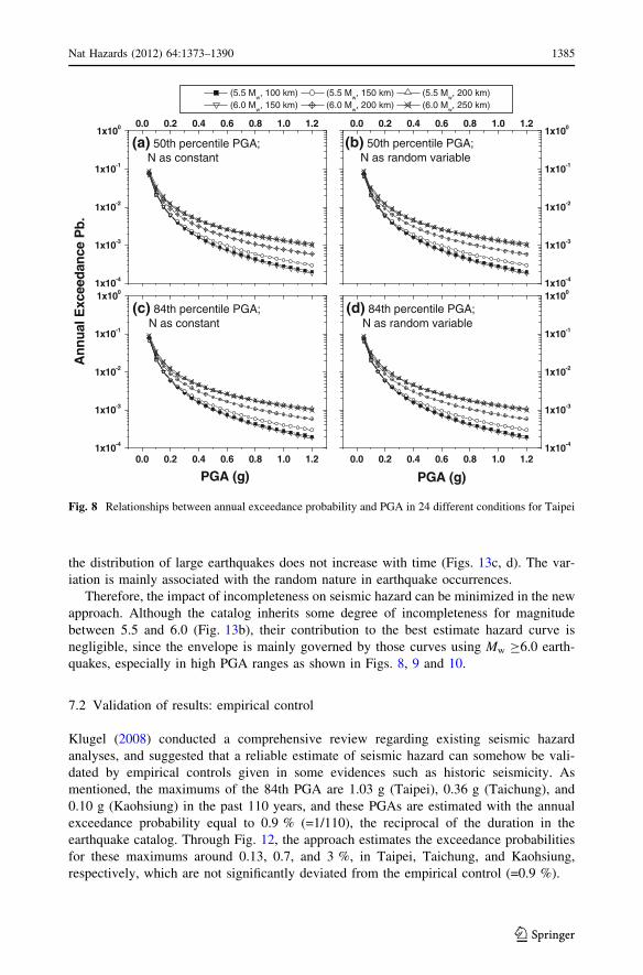
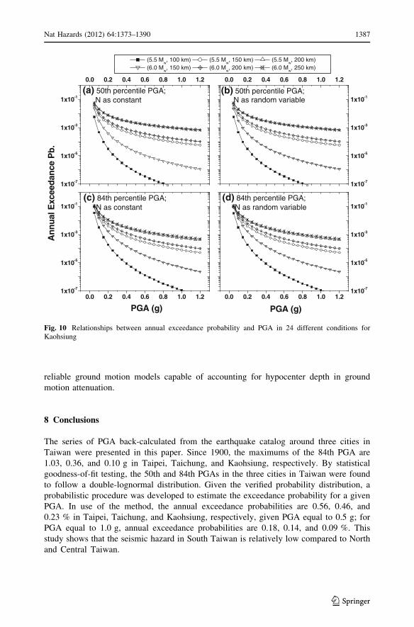
1x10-1 (d) 84th percentile PGA; N as random variable

(c) 84th percentile PGA; N as constant

(b) 50th percentile PGA; N as random variable

(a) 50th percentile PGA; N as constant

(5.5 Mw, 100 km) (5.5 M

w, 150 km) (5.5 M

w, 200 km)

(6.0 Mw, 150 km) (6.0 M

w, 200 km) (6.0 M

w, 250 km)

An

nu

al E

xcee

dan

ce P

b.

PGA (g) PGA (g)

Fig. 10 Relationships between annual exceedance probability and PGA in 24 different conditions forKaohsiung

Nat Hazards (2012) 64:1373–1390 1387

123

0.0 0.2 0.4 0.6 0.8 1.0 1.2

1x10-3

1x10-2

1x10-1

0.0 0.2 0.4 0.6 0.8 1.0 1.2

1x10-3

1x10-2

1x10-1

0.0 0.2 0.4 0.6 0.8 1.0 1.2

1x10-3

1x10-2

1x10-1

PGA (g)

(c) Kaohsiung

(b) Taichung

(a) Taipei

An

nu

alE

xcee

dan

ceP

rob

ailit

y

PGA50

; N as constant PGA50

; N as R.V.PGA

84; N as constant PGA

84; N as R.V.

Fig. 11 Highest seismic hazardcurves among those using sixdifferent thresholds (shown inFigs. 8, 9, 10)

0.0 0.2 0.4 0.6 0.8 1.0 1.2

1x10-3

1x10-2

1x10-1

An

nu

al E

xcee

dan

ce P

b.

PGA (g)

Taipei Taichung Kaohsiung

Fig. 12 Best estimate seismichazard for the three cities inTaiwan; the curves are developedby enveloping 24 analyses indifferent conditions (shown inFigs. 8, 9, 10)

1388 Nat Hazards (2012) 64:1373–1390

123

Acknowledgments The authors thank the Central Weather Bureau (CWB) Taiwan for providing theearthquake data. We also appreciate the valuable comments from anonymous reviewers.

References

Ang AH, Tang WH (2007) Probability concepts in engineering: emphasis on applications to civil andenvironmental engineering, 2nd edn. Wiley, New Jersey, pp 96–99 (112, 293-295)

Bommer JJ (2002) Deterministic versus probabilistic seismic hazard assessment: an exaggerated andobstructive dichotomy. J Earthq Eng 6(Special Issue 1):43–73

Bommer JJ (2003) Uncertainty about uncertainty in seismic hazard analysis. Eng Geol 70(1–2):165–168Castanos H, Lomnitz C (2002) PSHA: is it science? Eng Geol 66(3–4):315–317Cheng CT, Chiou SJ, Lee CT, Tsai YB (2007) Study on probabilistic seismic hazard maps of Taiwan after

Chi–Chi earthquake. J Eng Geol 2(1):19–28Cornell CA (1968) Engineering seismic risk analysis. Bull Seismol Soc Am 58(5):1583–1606Geller RJ, Jackson DD, Kagan YY, Mulargia F (1997) Earthquakes cannot be predicted. Science

275(5306):1616IAEA (2002) Evaluation of seismic hazards for nuclear power plants. Safety Guide NS-G-3.3, International

Atomic Energy Agency, ViennaJafari MA (2010) Statistical prediction of the next great earthquake around Tehran. Iran J Geodyn

49(1):14–18Kijko A, Sellevoll MA (1990) Estimation of earthquake hazard parameters for incomplete and uncertain

data files. Nat Hazards 3(1):1–13

1900 1920 1940 1960 1980 2000 2020

0

20

40

60

80

single year earthquake no. 5-yr moving average

(d) MW >= 6.5 (c) M

W >= 6.0

(b) MW >= 5.5 (a) M

W >= 5.0

0

5

10

15

20

25

30

0

2

4

6

8

10

12

No.

Ear

thqu

akes

No.

Ear

thq

uake

s

1900 1920 1940 1960 1980 2000

1900 1920 1940 1960 1980 2000 1900 1920 1940 1960 1980 2000

0

2

4

6

Year Year

Fig. 13 Temporal distribution of earthquakes: a Mw C 5.0, b Mw C 5.5, c Mw C 6.0, and d Mw C 6.5

Nat Hazards (2012) 64:1373–1390 1389

123

Klugel JU (2008) Seismic hazard analysis—Quo vadis? Earth Sci Rev 88(1–2):1–32Kramer SL (1996) Geotechnical Earthquake Engineering. Prentice Hall, New Jersey, pp 86–88 117-130Krinitzsky EL (1993a) Earthquake probability in engineering-part 1: the use and misuse of expert opinion:

the third Richard H. Jahns distinguished lecture in engineering geology. Eng Geol 33(3):219–231Krinitzsky EL (1993b) Earthquake probability in engineering-part 2: earthquake recurrence and limitations

of Guterberg-Richter b-values for the engineering of critical structures: the third Richard H. Jahnsdistinguished lecture in engineering geology. Eng Geol 36(1–2):1–52

Lin CW, Chen WS, Liu, YC, Chen PT (2009) Active faults of eastern and southern Taiwan. SpecialPublication of Central Geological Survey 23:178 (In Chinese with English Abstract)

Lin CW, Lu ST, Shih, TS, Lin WH, Liu YC, Chen PT (2008) Active faults of central Taiwan. SpecialPublication of Central Geological Survey 21:148 (In Chinese with English Abstract)

Sokolov VY, Wenzel F, Mohindra R (2009) Probabilistic seismic hazard assessment for Romania andsensitivity analysis: a case of joint consideration of intermediate-depth (Vrancea) and shallow (crustal)seismicity. Soil Dyn Earthq Eng 29(2):364–381

U.S. NRC (2007) Regulatory guide 1.208: A performance-based approach to define the site-specificearthquake ground motion. United States Nuclear Regulatory Commission, Washington

USGS (2008) National seismic hazard maps. United States Geological Survey, Virginia. http://earthquake.usgs.gov/hazards/

Wang JP, Chan CH, Wu YM (2011) The distribution of annual maximum earthquake magnitude aroundTaiwan and its application in the estimation of catastrophic earthquake recurrence probability. NatHazards 59(1):553–570

Wu YM, Kanamori H (2005a) Experiment on an onsite early warning method for the Taiwan early system.Bull Seismol Soc Am 95(1):347–354

Wu YM, Kanamori H (2005b) Rapid assessment of damaging potential of earthquakes in Taiwan from thebeginning of P waves. Bull Seismol Soc Am 95(3):1181–1185

Wu YM, Shin TC, Chang CH (2001) Near real-time mapping of peak ground acceleration and peak groundvelocity following a strong earthquake. Bull Seismol Soc Am 91(5):1218–1228

1390 Nat Hazards (2012) 64:1373–1390

123