213
| Date post: | 15-Apr-2017 |
| Category: |
Documents |
| Upload: | richard-buz |
| View: | 18 times |
| Download: | 1 times |

INFORMATION THEORETIC LIMITS ON
COMMUNICATION OVER MULTIPATH FADING
CHANNELS
by
Richard Buz
A thesis submitted to the Department of Electrical
Engineering in conformity with the requirements
for the degree of Doctor of Philosophy
Queen's University
Kingston, Ontario, Canada
June 1994
Copyright c Richard Buz, 1994

Abstract
While a considerable amount of research into the design of channel codes for use in
fading environments continues to be performed, it is done so without knowledge of
the magnitude of the potential gain yet to be achieved. Due to this circumstance, it is
uncertain as to whether the best known codes are actually any good when compared
to the class of all codes. In an attempt to remedy this situation, ultimate limits
on the rate of reliable communication over multipath fading channels are presented
here. These limits are based on the information theoretic notions of channel capacity
and average mutual information, and provide a benchmark against which to measure
the merit of any channel coding scheme. An idealized channel model is considered
�rst, and through comparison with known results for additive noise channels, the
loss due to amplitude fading is determined. Channels with continuous-valued input
alphabets are considered as well as those based on practical signal constellations.
Information theoretic limits are determined when subject to both average and peak
power constraints, the latter being more relevant to mobile communication. While
multiple antennae are commonly used to combat channel loss, the e�ect of this space
diversity is viewed here from an information theoretic perspective, and the resulting
gain in the rate of reliable data transmission is ascertained. The magnitude of the
potential gain over uncoded modulation achievable through the use of signal shaping
and channel coding is stated.
In conjunction with the in uence of amplitude fading, the performance of any prac-
ticable communication strategy is also a�ected by imperfect channel state estimation
as well as time dispersion of the transmitted signal. Each of these considerations is
addressed separately, through augmentation of the idealized channel model, in order
ii

to ascertain their e�ect on the maximum rate of reliable data transmission. The re-
quirement of channel estimation is demonstrated through calculation of information
theoretic limits for channels in which the state of the fading process is unknown.
Similar results are also obtained for the case of perfect coherent detection with no
knowledge of the fading amplitude. Through comparison with results obtained for the
ideal channel, the losses incurred due to the limitation of practical channel estimation
schemes is determined. The particular methods of channel estimation considered are
pilot tone extraction, di�erentially coherent detection, and the use of a pilot sym-
bol. The e�ect of time dispersion is examined through calculation of the capacity
of a frequency-selective fading channel represented by the two-path Rayleigh model.
An inherent time diversity e�ect is demonstrated, which manifests itself in certain
instances of frequency-selective fading.
iii

Acknowledgements
Most people that I meet are under the impression that a Ph.D. is some type of
honor bestowed upon people with superior intellect. I always tell them that the
process of obtaining a doctorate has little to do with intelligence and is more like a
test of endurance. Although I believe this somewhat facetious statement re ects one
important requirement, there were other equally vital contributing factors involved
in the realization of this thesis.
I am indebted to Dr. Peter McLane for inspiring my interest in communications
and for providing the opportunity to accomplish this project. I appreciate the con�-
dence that he showed in my abilities and the patience he exhibited in waiting for me
to get things done.
Funding of this research was provided in part by both the Natural Sciences and
Engineering Research Council of Canada and the Canadian Institute for Telecom-
munications Research. The Telecommunications Research Institute of Ontario also
contributed �nancial support as well as the use of computer facilities. I would like to
express my gratitude to these organizations for their assistance.
I would like to thank Dr. Norman Beaulieu and Dr. Lorne Campbell for repeat-
edly sharing their insight with me whenever I would drop by unannounced with a
mathematical problem.
I can never thank my parents enough. They exhibited the value of hard work to
me and always encouraged me to set my goals high. It was a comfort to know that
they were always there for me, willing to help whenever I needed them.
Finally, it was William Shakespeare, who through his play \King Lear", instilled
the belief in my mind that it's better to go mad than to give up.
iv

Summary of Notation
Abbreviations
AMI average mutual information
AMPM amplitude modulation / phase modulation
AWGN additive white Gaussian noise
BCM block coded modulation
bps bits per second
CSI channel state information
CR cross constellation
dB decibel
DPSK di�erential phase shift keying
Hz hertz
kbps kilobits per second
kHz kilohertz
LOS line-of-sight
MHz megahertz
mph miles per hour
MSAT mobile satellite
MTCM multiple trellis coded modulation
NASA National Aeronautics and Space Administration
PAR peak-to-average power ratio
pdf probability density function
pmf probability mass function
PSK phase shift keying
v

QAM quadrature amplitude modulation
QPSK quaternary phase shift keying
SNR signal-to-noise power ratio
TCM trellis coded modulation
Symbols and Functions
A signal amplitude
ai weighting coeÆcient
a(t) envelope of transmitted signal
BD Doppler spread of channel
(B)ij entry in covariance matrix
B covariance matrix
C channel capacity
Cxy correlation between random variables x and y
CE Euler's constant
d Euclidean distance
Eb average received energy per bit
Es average received symbol energy
EX average power of a random variable X
E f�g operator denoting statistical expectation
Ei(�) exponential integral function
erf(�) error function
erfc(�) complimentary error function
FW water pouring band
fc carrier frequency
fD Doppler frequency
G(f) inverse of channel SNR function
GF (�) Galois �eld
g(t) baseband pulse
vi

H(f) channel transfer function
H(�) entropy of a random variable
H(�j�) conditional entropy
h(t) channel impulse response
I(�; �) average mutual information
I0(�) modi�ed Bessel function of �rst kind and zero order
IW water pouring band for parallel channels
=f�g imaginary part of enclosed complex number
J(�) Jacobian of coordinate transformation
J0(�) Bessel function of �rst kind and zero order
j square root of -1
K0 threshold for water pouring
L level of diversity
Lf�g Laplace transform operator
M size of signal set
m Nakagami channel parameter
mX mean value of a random variable X
N random noise variable
N0 noise power spectral density
NB length of a block of channel symbols
N(f) general noise power spectral density
n(t) random noise process
P average transmitted power
Pb bit error probability
Ps peak power of constellation
Pr(e) probability of detection error
PX entropy power of a random variable X
p(�) probability density function
p(�j�) conditional probability density function
R random fading amplitude variable
R0 computational cuto� rate
vii
Rc rate of transmission
Rh(�) multipath intensity pro�le of channel
Rx(�) auto-correlation function of a random process x(t)
<f�g real part of enclosed complex-valued expression
ri(t) attenuation along ith propagation path
SX support set of a random variable X
Sh(�) Doppler power spectrum of channel
SX(f) power spectral density of signal x(t)
s(t) transmitted bandpass signal
T duration of channel symbol
T transpose of matrix
Tm multipath spread of channel
Ts duration of signal
u(t) complex envelope of transmitted signal
v velocity of mobile unit
W bandwidth of transmit spectrum
Wp bandwidth of pilot tone extraction �lter
X channel input alphabet
x di�erentially encoded channel symbol
xp pilot symbol
Y channel output alphabet
y(t) baseband signal at receiver
yi(t) signal received by ith antenna
�(�) gamma function or generalized factorial
power ratio
R Rician channel parameter
�J discrepancy in Jensen's inequality
(�f)H coherence bandwidth of channel
(�t)h coherence time of channel
Æ(�) Dirac delta function
�A angle of asymmetry
viii

�(t) phase of transmitted signal
� carrier wavelength
� correlation coeÆcient
�2X variance of a random variable X
�i(t) delay along ith propagation path
� random fading variable
~� estimate of fading variable at receiver
�(t) random fading process
� random fading phase variable
�i(t) phase shift along ith propagation path
'i(t) function from an orthonormal set
angle of incidence
(�) Euler's psi function
second moment of Nakagami fading variable
! radian frequency
d�e smallest integer greater than the enclosed value
ix

Contents
Abstract ii
Acknowledgements iv
Summary of Notation v
List of Tables xiv
List of Figures xvi
1 Introduction 1
1.1 Lessons Learned from the AWGN Channel . . . . . . . . . . . . . . . 2
1.2 State of the Art Coding for Fading Channels . . . . . . . . . . . . . . 5
1.3 Known Applications of Information Theory to Fading Channels . . . 10
1.4 Contributions of Thesis . . . . . . . . . . . . . . . . . . . . . . . . . . 11
1.5 Presentation Outline . . . . . . . . . . . . . . . . . . . . . . . . . . . 12
2 Multipath Fading Channel Models 14
2.1 The Physical Channel . . . . . . . . . . . . . . . . . . . . . . . . . . 14
2.2 Amplitude Fading Models . . . . . . . . . . . . . . . . . . . . . . . . 20
2.2.1 Rayleigh Fading . . . . . . . . . . . . . . . . . . . . . . . . . . 21
2.2.2 Rician Fading . . . . . . . . . . . . . . . . . . . . . . . . . . . 22
2.2.3 Shadowed Rician Fading . . . . . . . . . . . . . . . . . . . . . 22
2.2.4 Nakagami Fading . . . . . . . . . . . . . . . . . . . . . . . . . 23
2.3 E�ects of Frequency Dispersion . . . . . . . . . . . . . . . . . . . . . 24
2.3.1 Symbol Interleaving . . . . . . . . . . . . . . . . . . . . . . . . 24
x

2.3.2 Diversity Combining . . . . . . . . . . . . . . . . . . . . . . . 25
2.3.3 Channel State Estimation . . . . . . . . . . . . . . . . . . . . 27
2.4 Frequency-Selective Fading Channels . . . . . . . . . . . . . . . . . . 29
2.4.1 Linear Filter Model . . . . . . . . . . . . . . . . . . . . . . . . 29
2.4.2 Three-Path Model . . . . . . . . . . . . . . . . . . . . . . . . 30
2.4.3 Two-Path Rayleigh Model . . . . . . . . . . . . . . . . . . . . 33
3 Information Theoretic Bounds for Ideal Fading Channels 35
3.1 Information Theoretic Concepts . . . . . . . . . . . . . . . . . . . . . 36
3.2 Channels with Discrete-Valued Input . . . . . . . . . . . . . . . . . . 44
3.2.1 Standard Signal Constellations . . . . . . . . . . . . . . . . . 47
3.2.2 Asymmetric PSK Constellations . . . . . . . . . . . . . . . . . 53
3.3 Capacity of Ideal Fading Channels . . . . . . . . . . . . . . . . . . . 56
3.4 Peak Power Considerations . . . . . . . . . . . . . . . . . . . . . . . . 65
3.4.1 Peak Power Results for Discrete-Valued Input . . . . . . . . . 65
3.4.2 Channel Capacity with a Peak Power Constraint . . . . . . . . 72
3.5 Channels with Space Diversity . . . . . . . . . . . . . . . . . . . . . . 76
3.5.1 E�ect of Diversity on Discrete-Input Channels . . . . . . . . . 79
3.5.2 Capacity of Fading Channels with Space Diversity . . . . . . . 87
3.6 Potential Coding Gain for Fading Channels . . . . . . . . . . . . . . . 94
4 E�ects of Non-Ideal Channel State Information 100
4.1 Requirement of Channel State Estimation . . . . . . . . . . . . . . . 101
4.1.1 Channels with Discrete-Valued Input and No CSI . . . . . . . 101
4.1.2 Channel with Continuous-Valued Input and No CSI . . . . . . 104
4.2 Channels with Phase-Only Information . . . . . . . . . . . . . . . . . 109
4.2.1 Phase-Only Channels with Discrete-Valued Input . . . . . . . 111
4.2.2 Phase-Only Channels with Continuous-Valued Input . . . . . 120
4.3 Realistic Channel Estimation Methods . . . . . . . . . . . . . . . . . 122
4.3.1 Channel Estimation Via Pilot Tone Extraction . . . . . . . . . 126
4.3.2 Channel Estimation Via Di�erentially Coherent Detection . . 133
4.3.3 Channel Estimation Via Pilot Symbol Transmission . . . . . . 140
xi

5 Information Theoretic Bounds for Frequency-Selective Fading Chan-
nels 146
5.1 Representation of Waveform Channels . . . . . . . . . . . . . . . . . 147
5.1.1 Time-Invariant Filter Channels . . . . . . . . . . . . . . . . . 150
5.2 Capacity of the Two-Path Rayleigh Channel . . . . . . . . . . . . . . 152
5.2.1 Properties of the Two-Path Model . . . . . . . . . . . . . . . 154
5.2.2 Capacity and Equalization . . . . . . . . . . . . . . . . . . . . 156
5.3 Time Diversity E�ect . . . . . . . . . . . . . . . . . . . . . . . . . . . 156
5.3.1 Channels with Discrete-Valued Input . . . . . . . . . . . . . . 158
5.3.2 Channels with Continuous-Valued Input . . . . . . . . . . . . 164
6 Conclusion 168
6.1 Summary of Presentation . . . . . . . . . . . . . . . . . . . . . . . . . 168
6.2 Conclusions . . . . . . . . . . . . . . . . . . . . . . . . . . . . . . . . 170
6.3 Suggestions for Further Research . . . . . . . . . . . . . . . . . . . . 172
Bibliography 174
A Comment on Results Obtained Through Computer Simulation 180
B Calculation of Channel Capacity for Speci�c Fading Distributions 181
B.1 Capacity of a Rayleigh Fading Channel . . . . . . . . . . . . . . . . . 181
B.2 Capacity of a Nakagami Fading Channel . . . . . . . . . . . . . . . . 182
C Calculation of Asymptotic Loss Due to Speci�c Fading Distributions184
C.1 Asymptotic Loss Due to Rayleigh Fading . . . . . . . . . . . . . . . . 184
C.2 Asymptotic Loss Due to Nakagami Fading . . . . . . . . . . . . . . . 185
D Calculation of Error Probability for Uncoded Modulation in Ideal
Rayleigh Fading 187
D.1 Symbol Error Probability for Uncoded QAM . . . . . . . . . . . . . . 187
D.2 Bit Error Probability for Uncoded QPSK . . . . . . . . . . . . . . . . 190
E Derivation of a PDF Related to the Two-Path Rayleigh Channel 192
xii

Vita 194
xiii

List of Tables
3.1 Minimum SNR Required for Various Rates of AMI on an AWGN Chan-
nel: PSK Constellations . . . . . . . . . . . . . . . . . . . . . . . . . 45
3.2 Minimum SNR Required for Various Rates of AMI on an AWGN Chan-
nel: QAM Constellations . . . . . . . . . . . . . . . . . . . . . . . . . 45
3.3 Minimum SNR Required for Various Rates of AMI on an Ideal Rayleigh
Fading Channel: PSK Constellations . . . . . . . . . . . . . . . . . . 51
3.4 Minimum SNR Required for Various Rates of AMI on an Ideal Rayleigh
Fading Channel: QAM Constellations . . . . . . . . . . . . . . . . . . 51
3.5 Loss of SNR Due to Rayleigh Fading: PSK Constellations . . . . . . 52
3.6 Loss of SNR Due to Rayleigh Fading: QAM Constellations . . . . . . 52
3.7 Average Power Gain Due to Increase in Space Diversity of Rayleigh
Fading Channel . . . . . . . . . . . . . . . . . . . . . . . . . . . . . . 81
3.8 Average Power Loss Due to Space Correlation of the Fading Process . 84
4.1 Loss of SNR Due to Phase-Only Information: PSK Constellations . . 114
4.2 Loss of SNR Due to Phase-Only Information: QAM Constellations . . 116
4.3 Loss of SNR Due to Phase-Only Information: Hybrid AMPM Constel-
lations . . . . . . . . . . . . . . . . . . . . . . . . . . . . . . . . . . . 118
4.4 Loss of SNR Due to Non-Ideal CSI: Pilot Tone Estimation with PSK
Constellations . . . . . . . . . . . . . . . . . . . . . . . . . . . . . . . 133
4.5 Loss of SNR Due to Non-Ideal CSI: Pilot Tone Estimation with QAM
Constellations . . . . . . . . . . . . . . . . . . . . . . . . . . . . . . . 134
4.6 Loss of SNR Due to Non-Ideal CSI: Di�erentially Coherent Detection
with PSK Constellations . . . . . . . . . . . . . . . . . . . . . . . . . 139
xiv

4.7 Loss of SNR Due to Non-Ideal CSI: Pilot Symbol Transmission . . . . 145
5.1 Gain Due to Time Diversity E�ect on the Two-Path Rayleigh Channel 163
xv
List of Figures
2.1 Multipath Fading Environment . . . . . . . . . . . . . . . . . . . . . 16
2.2 Channel Transfer Function of the Three-Path Model . . . . . . . . . . 32
3.1 AMI of an AWGN Channel: PSK Constellations . . . . . . . . . . . . 42
3.2 AMI of an AWGN Channel: QAM Constellations . . . . . . . . . . . 43
3.3 AMI of an Ideal Rayleigh Fading Channel: PSK Constellations . . . . 49
3.4 AMI of an Ideal Rayleigh Fading Channel: QAM Constellations . . . 50
3.5 AMI of an Ideal Rayleigh Fading Channel: Asymmetric PSK Constel-
lations . . . . . . . . . . . . . . . . . . . . . . . . . . . . . . . . . . . 55
3.6 Capacity of an Ideal Rayleigh Fading Channel . . . . . . . . . . . . . 59
3.7 Capacity of an Ideal Rician Fading Channel . . . . . . . . . . . . . . 61
3.8 Capacity of an Ideal Shadowed Rician Fading Channel . . . . . . . . 63
3.9 Capacity of an Ideal Nakagami Fading Channel . . . . . . . . . . . . 64
3.10 AMI of an Ideal Rayleigh Fading Channel in Terms of Peak Power:
QAM Constellations . . . . . . . . . . . . . . . . . . . . . . . . . . . 67
3.11 Hybrid AMPM Constellations . . . . . . . . . . . . . . . . . . . . . . 69
3.12 AMI of an Ideal Rayleigh Fading Channel in Terms of Average Power:
Hybrid AMPM Constellations . . . . . . . . . . . . . . . . . . . . . . 70
3.13 AMI of an Ideal Rayleigh Fading Channel in Terms of Peak Power:
Hybrid AMPM Constellations . . . . . . . . . . . . . . . . . . . . . . 71
3.14 Bounds on the Capacity of an Ideal Rayleigh Fading Channel with a
Peak Power Constraint . . . . . . . . . . . . . . . . . . . . . . . . . . 77
3.15 AMI of an Ideal Rayleigh Fading Channel with Space Diversity: 8-PSK 82
3.16 AMI of an Ideal Rayleigh Fading Channel with Space Diversity: 16-QAM 83
xvi
3.17 AMI of an Ideal Rayleigh Fading Channel with Diversity=2 and Space
Correlated Fading: 8-PSK . . . . . . . . . . . . . . . . . . . . . . . . 85
3.18 AMI of an Ideal Rayleigh Fading Channel with Diversity=2 and Space
Correlated Fading: 16-QAM . . . . . . . . . . . . . . . . . . . . . . . 86
3.19 Capacity of an Ideal Rayleigh Fading Channel with Space Diversity . 91
3.20 Capacity of Dual Diversity Rayleigh Channel with Space Correlated
Fading . . . . . . . . . . . . . . . . . . . . . . . . . . . . . . . . . . . 93
3.21 Probability of Symbol Error for Uncoded QAM in Rayleigh Fading . 96
3.22 Bit Error Probability in Rayleigh Fading for Various Coded Modulation
Schemes with Rate 2 bits/T . . . . . . . . . . . . . . . . . . . . . . . 97
3.23 Bit Error Probability in Rayleigh Fading for Turbo Codes . . . . . . 99
4.1 AMI of a Rician Fading Channel with No CSI: 8-PSK . . . . . . . . . 105
4.2 AMI of a Rician Fading Channel with No CSI: 16-QAM . . . . . . . . 106
4.3 Upper Bounds on the AMI of a Rician Fading Channel with No CSI:
Gaussian Distributed Input . . . . . . . . . . . . . . . . . . . . . . . 110
4.4 AMI of a Phase-Only Rayleigh Fading Channel: PSK Constellations . 115
4.5 AMI of a Phase-Only Rayleigh Fading Channel: QAM Constellations 117
4.6 AMI of a Phase-Only Rayleigh Fading Channel: Hybrid AMPM Con-
stellations . . . . . . . . . . . . . . . . . . . . . . . . . . . . . . . . . 119
4.7 Bounds on AMI for a Phase-Only Rayleigh Channel with Continuous-
Valued Input . . . . . . . . . . . . . . . . . . . . . . . . . . . . . . . 123
4.8 AMI of Rayleigh Fading Channel with CSI Provided Via Pilot Tone
Extraction: 8-PSK . . . . . . . . . . . . . . . . . . . . . . . . . . . . 129
4.9 AMI of Rayleigh Fading Channel with CSI Provided Via Pilot Tone
Extraction: 16-PSK . . . . . . . . . . . . . . . . . . . . . . . . . . . . 130
4.10 AMI of Rayleigh Fading Channel with CSI Provided Via Pilot Tone
Extraction: 16-QAM . . . . . . . . . . . . . . . . . . . . . . . . . . . 131
4.11 AMI of Rayleigh Fading Channel with CSI Provided Via Pilot Tone
Extraction: 32-CR . . . . . . . . . . . . . . . . . . . . . . . . . . . . 132
4.12 AMI of Rayleigh Fading Channel with CSI Provided Via Di�erentially
Coherent Detection: 8-PSK . . . . . . . . . . . . . . . . . . . . . . . 137
xvii

4.13 AMI of Rayleigh Fading Channel with CSI Provided Via Di�erentially
Coherent Detection: 16-PSK . . . . . . . . . . . . . . . . . . . . . . . 138
4.14 AMI of Rayleigh Fading Channel with CSI Provided Via Pilot Symbol
Transmission: 8-PSK . . . . . . . . . . . . . . . . . . . . . . . . . . . 143
4.15 AMI of Rayleigh Fading Channel with CSI Provided Via Pilot Symbol
Transmission: 16-QAM . . . . . . . . . . . . . . . . . . . . . . . . . . 144
5.1 AMI for Two-Path Rayleigh Fading Channel with Time Diversity Ef-
fect: 8-PSK . . . . . . . . . . . . . . . . . . . . . . . . . . . . . . . . 161
5.2 AMI for Two-Path Rayleigh Fading Channel with Time Diversity Ef-
fect: 16-QAM . . . . . . . . . . . . . . . . . . . . . . . . . . . . . . . 162
5.3 Capacity of Two-Path Rayleigh Fading Channel with Time Diversity
E�ect . . . . . . . . . . . . . . . . . . . . . . . . . . . . . . . . . . . 167
xviii

Chapter 1
Introduction
At the present time it's becoming rare to �nd any communications related publication
that does not make reference to the \wireless revolution". This revolution has wit-
nessed the realization of a number of mobile communication systems; some examples
of which are mobile satellite, cellular telephone, and personal communication services.
What these schemes have in common is that the transmission medium for commu-
nication is accurately modelled as a multipath fading channel. Due to a continuing
dramatic increase in the use of these systems, as well as the need for standardiza-
tion of the methods used, a considerable amount of research has been directed at the
development of eÆcient strategies for transmitting data over fading channels.
Prior to the wireless revolution, a signi�cant amount of research was focussed on
achieving reliable communication over telephone lines. These telephone line chan-
nels are well-modelled by the sequential combination of a linear �lter followed by
an additive noise process. The noise is usually described as being a spectrally- at
Gaussian random process, and the transmission medium is referred to as an additive
white Gaussian noise (AWGN) channel. The limits of communication over AWGN
channels were determined �rst, and it was not until four decades later that research
in equalization and channel coding allowed these limits to be approached.
The techniques developed for communication over AWGN channels have been
applied to fading channels; however, performance of these techniques in fading is
signi�cantly inferior to additive noise channel results. Much of the research currently
being performed deals with the modi�cation of known channel coding techniques for
1

use over fading channels. So far some great improvements have been made, but
data rates achievable in fading are still quite modest in comparison to telephone
line channels. Due to the extreme di�erence in reliability between fading and noise
channels, one cannot help asking certain fundamental questions. Must performance in
fading be so inferior to the results obtained for the additive noise channel? Although
a new code may result in an improvement over all other known codes, does this mean
that the new one is actually a good code? Until the limits of communication over
multipath fading channels are determined, these questions cannot be answered.
1.1 Lessons Learned from the AWGN Channel
Prior to 1948, most engineers believed that the noise present on a communication
channel placed a limit on the reliability of transmitting data. No matter what solu-
tions were used to combat the noise, most concurred that this perceived limit could
not be surpassed. These engineers learned that this was not the case after the appear-
ance of Claude Shannon's seminal work [1], which gave birth to the �eld of information
theory. Using Hartley's quantitative measure of information [2] and ideas from sta-
tistical mechanics, Shannon developed a number of momentous results. One of these
results, known as the channel coding theorem, states that under certain conditions
there is no �xed limit on the reliability of communication. Given a particular channel
model, there exists a maximum rate of transmission called the capacity of the chan-
nel. The channel coding theorem states that as long as the transmission rate does
not exceed the channel capacity, there exists some coding scheme which can be used
to achieve an arbitrary degree of reliability. For an ideal AWGN channel bandlimited
to W Hz, and a signal-to-noise power ratio denoted by SNR, the capacity measured
in bits per second is given by the formula [1]
C =W log2 (1 + SNR) bps: (1.1)
When using uncoded QAM signal sets to transmit data over a high-SNR AWGN
channel, a symbol error rate of the order of 10�5�10�6 is achieved at a SNR which is
9 dB greater than that given by the capacity formula [3]. An alternate interpretation
of this result is that there is an additional 3 bps/Hz to be gained in the data rate
2
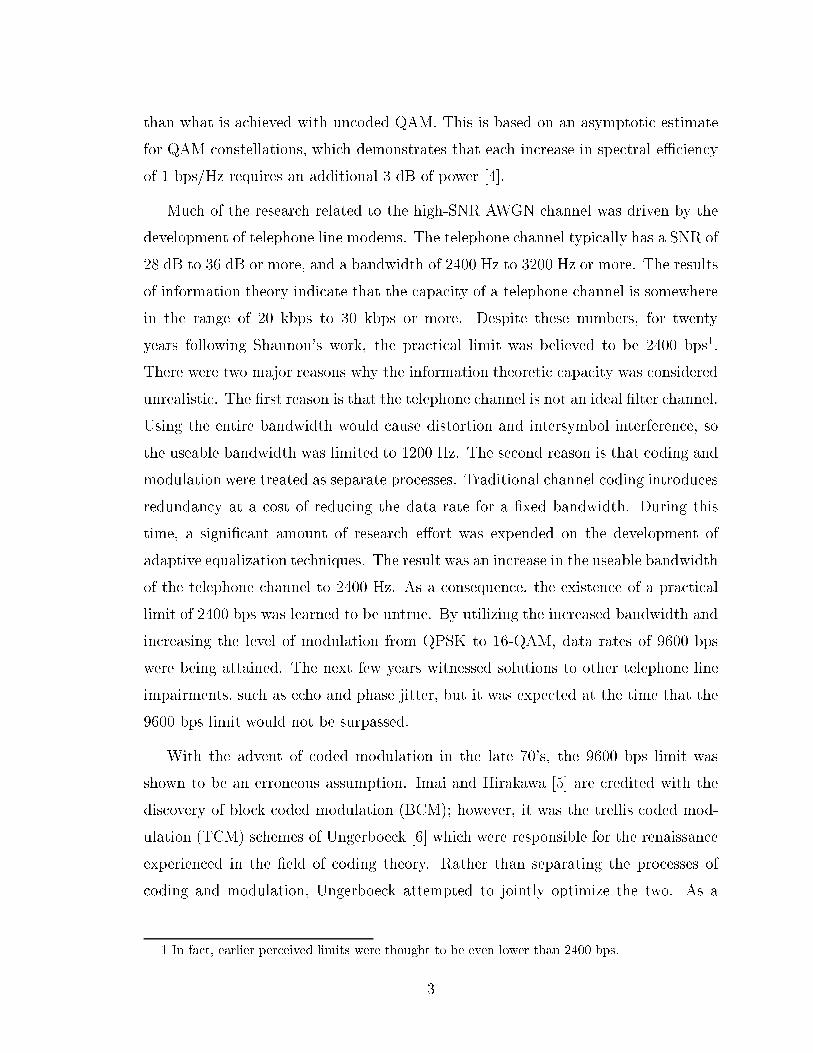
than what is achieved with uncoded QAM. This is based on an asymptotic estimate
for QAM constellations, which demonstrates that each increase in spectral eÆciency
of 1 bps/Hz requires an additional 3 dB of power [4].
Much of the research related to the high-SNR AWGN channel was driven by the
development of telephone line modems. The telephone channel typically has a SNR of
28 dB to 36 dB or more, and a bandwidth of 2400 Hz to 3200 Hz or more. The results
of information theory indicate that the capacity of a telephone channel is somewhere
in the range of 20 kbps to 30 kbps or more. Despite these numbers, for twenty
years following Shannon's work, the practical limit was believed to be 2400 bps1.
There were two major reasons why the information theoretic capacity was considered
unrealistic. The �rst reason is that the telephone channel is not an ideal �lter channel.
Using the entire bandwidth would cause distortion and intersymbol interference, so
the useable bandwidth was limited to 1200 Hz. The second reason is that coding and
modulation were treated as separate processes. Traditional channel coding introduces
redundancy at a cost of reducing the data rate for a �xed bandwidth. During this
time, a signi�cant amount of research e�ort was expended on the development of
adaptive equalization techniques. The result was an increase in the useable bandwidth
of the telephone channel to 2400 Hz. As a consequence, the existence of a practical
limit of 2400 bps was learned to be untrue. By utilizing the increased bandwidth and
increasing the level of modulation from QPSK to 16-QAM, data rates of 9600 bps
were being attained. The next few years witnessed solutions to other telephone line
impairments, such as echo and phase jitter, but it was expected at the time that the
9600 bps limit would not be surpassed.
With the advent of coded modulation in the late 70's, the 9600 bps limit was
shown to be an erroneous assumption. Imai and Hirakawa [5] are credited with the
discovery of block coded modulation (BCM); however, it was the trellis coded mod-
ulation (TCM) schemes of Ungerboeck [6] which were responsible for the renaissance
experienced in the �eld of coding theory. Rather than separating the processes of
coding and modulation, Ungerboeck attempted to jointly optimize the two. As a
1 In fact, earlier perceived limits were thought to be even lower than 2400 bps.
3

result, simple practical codes were discovered which e�ected gains of 3-4 dB with-
out a reduction in data rate, while up to 6 dB of gain was reached by using more
complex codes. With regard to coded modulation, redundancy is added to the data
by expanding the size of the required signal set. Channel symbols are then assigned
to code sequences in a manner that ensures that the gain in distance between signal
sequences is greater than the power loss incurred due to signal set expansion2. One
method of accomplishing this is Ungerboeck's technique of mapping by set partition-
ing. Modi�ed versions of Ungerboeck's codes were included in modem standards in
the mid 1980's for data rates of up to 14.4 kbps [7].
Although Calderbank and Sloane [8] are credited with introducing the language of
lattices and cosets to coded modulation, it was Forney's comprehensive work on coset
codes [9] that placed coded modulation on a �rm mathematical basis, and allowed
a more profound understanding of the subtleties of code structure. One of Forney's
observations was that the total gain obtained could be separated into two relatively
independent terms. The �rst term is called the shaping gain, and has an ultimate limit
of 1.53 dB. Shaping gain is obtained when spherical multi-dimensional constellations
are utilized rather than cubic ones. The second term is referred to as the coding gain.
With respect to the 9 dB di�erence between the error performance of QAM and the
capacity of a high-SNR AWGN channel, since shaping can theoretically be used to
reduce the gap by about 1.5 dB, the remaining 7.5 dB represents the limit for the
maximum coding gain to be achieved. Forney also observed that after the �rst 5-6 dB
of coding gain is acquired, it is easier to obtain the next 1 dB by shaping rather than
by using a more complex code [10]. The combination of these realizable gains places
practical results at less than 3 dB from the theoretical limit. At present, standards
are being determined for modems to transmit data over telephone channels at rates
of 19.2 kbps or higher. By incorporating precoding, channel coding, and shaping in
modem design, the Codex corporation claims to have achieved reliable transmission
at a rate of 24 kbps [11]. Many of the facts contained in this section have been taken
from [11], which contains a more detailed history of telephone line modems.
Another recently published paper [12], although not related to coded modulation,
2 This power loss refers to the increase in average power required to maintain the minimumdistance between channel symbols when increasing the size of the constellation.
4

presents a traditional coding scheme which yields a bit error probability of 10�5 at
only 0.7 dB from the theoretical capacity of the channel. This scheme uses a parallel
concatenation of two 16-state recursive systematic convolutional codes. An iterative
decoding algorithm is utilized, where performance improves in relation to the number
of iterations carried out.
It seems that even though approaching channel capacity was once considered an
impractical goal, knowledge of this limit must have left the impression on some that
there was always more to be gained. With each increase obtained in the data rate,
the theoretical channel capacity has always been a constant goal to strive for.
1.2 State of the Art Coding for Fading Channels
At present, the reliable high data rate communications available on telephone line
channels cannot be achieved over multipath fading channels. There are a number of
factors which contribute to this limitation. One reason is that there are more potential
sources of signal degradation associated with fading environments. For example,
multipath fading and Doppler spread can have deleterious e�ects on communication.
Another reason is that most error correcting codes have been designed to correct
random errors, whereas on a fading channel, errors tend to occur in bursts. These
error bursts arise during deep fades, which cause the signal to become more susceptible
to noise. Another important consideration for many systems used in fading is the
presence of non-linear distortion. Satellite transponders, as well as most cost eÆcient
ampli�ers, are usually operated in a mode that causes them to have a non-linear
characteristic. In this case, constant envelope signalling methods such as PSK or
continuous phase modulation must be used in order to avoid the e�ects of distortion
and bandwidth expansion caused by non-linearities. In terrestrial microwave systems,
the availability of power permits the use of linear ampli�ers, which in turn allows the
use of higher levels of QAM. It is easier to increase the bandwidth eÆciency of linear
channels, since high level QAM outperforms high level PSK modulation with regard
to average signal power.
In order to increase power eÆciency, traditional coding could be used by trading
5

o� bandwidth or data rate. This is obviously diÆcult for satellite communication
systems, which are already constrained to have a lower data rate due to the use of
constant envelope modulation. At present, however, traditional coding techniques
are the only ones which have actually been used over fading channels. The most
popular coding methods adopted for satellite and deep space communications are
convolutional codes and Reed Solomon codes [13]. The standard convolutional codes
used are of rate 12or 2
3, and usually have 64 or 128 encoder states. The standard Reed
Solomon code used by NASA is a (255, 233) code over GF (28) [14]. Reed Solomon
codes are designed to correct burst errors, while convolutional codes are used to
combat random errors. Sometimes the two techniques are concatenated so that data
is protected from both types of error distribution. The constant envelope modulation
generally used in fading is QPSK. Due to the diÆculty in achieving accurate coherent
transmission over mobile fading channels, di�erential encoding is often used in the
transmitter along with di�erentially coherent detection in the receiver. In this case,
the modulation method is referred to as di�erential phase shift keying (DPSK).
It seems that the satellite channel would be a prime area of application for band-
width eÆcient trellis coded modulation. In fact, this is where most of the initial
research was done in the application of coded modulation to fading channels. In par-
ticular, the mobile satellite (MSAT) systems developed in Canada [15] and the United
States [16] were the �rst particular projects which prompted work in this area. Initial
research was aimed at achieving high quality voice transmission over fading channels.
Telephone line quality digital voice transmission requires an average bit error rate of
10�3. In [15], the study used a rate of 1200 symbols per second to obtain a bit rate
of 2400 bps. The MSAT channel was originally proposed to be bandlimited to about
5 kHz, and data rates of 4800 to 9600 bps were of interest in [16]. In both cases, a
maximum spectral eÆciency of 2 bits/T was considered3. Due to the non-linearity
of the satellite channel, constant envelope QPSK and 8-PSK symbol sets were used.
Computer simulations as well as upper bounds on error probability were presented
to indicate code performance. These results included practical considerations such as
3 The parameter T represents the duration of a channel symbol. The spectral eÆciency in unitsof bps/Hz may be determined through multiplication by the number of channel symbols transmittedper Hz of bandwidth.
6

�nite symbol interleaving, di�erential encoding, and the e�ects of non-ideal channel
state information. While still signi�cantly inferior to AWGN channel results, the use
of TCM resulted in tremendous gains over uncoded schemes for use in fading, with
no reduction in data rate. For the AWGN channel, codes are designed to maximize
the minimum Euclidean distance between symbol sequences. When fading channels
are considered, however, it was discovered that codes with parallel trellis transitions
are inferior to those without, even when the minimum Euclidean distance is greater.
For those codes without parallel transitions, Ungerboeck's 8-PSK codes [6] proved
to be superior. Some small additional gains were obtained in [16] by introducing
asymmetry into the PSK constellations used in order to increase the minimum Eu-
clidean distance between code sequences. For the Canadian MSAT system, despite
the promising performance of TCM, a traditional convolutional code used in com-
bination with QPSK modulation was �nally accepted in the standard. In order to
compensate for the loss in data rate due to coding, the bandwidth was increased to
7500 Hz.
In [17], Divsalar and Simon set out performance criteria for the design of TCM
for fading channels. This was done through examination of an expression which
is an upper bound on the probability of bit error. For high values of SNR, the
most important factor in code design is the minimum time diversity between code
sequences. Time diversity refers to the number of signalling intervals in which symbols
di�er between code sequences. For large values of SNR, the bit error probability
decreases in proportion to (SNR)�L, where L is the minimum time diversity between
all code sequences. This explains why Ungerboeck codes with parallel transitions are
not good for use over fading channels. A diversity of 1 symbol would result in an
inverse linear decrease in error probability with respect to SNR. The second design
criterion is to maximize the minimum product distance between sequences. The
product distance is the product of the non-zero squared Euclidean distances between
corresponding symbols in a pair of code sequences. Bit error probability has an inverse
dependence on the product distance. The third criterion is to maximize the minimum
Euclidean distance between code sequences, which is the most important criterion for
the AWGN channel. The minimum Euclidean distance has a more signi�cant e�ect on
7

error performance when there is a line-of-sight path from transmitter to receiver, or
when the fading process does not appear completely independent between symbols at
the receiver. It is interesting to note that when using traditional coding, maximizing
Hamming distance also maximizes diversity between code sequences. Unfortunately,
this is not the case with coded modulation, which uses a Euclidean distance metric.
Multidimensional QAM constellations were �rst used in trellis codes for the tele-
phone channel [18]. The analog using PSK signal sets was called multiple trellis coded
modulation (MTCM) in [19]. Also presented in [20], MTCM was shown to attain a
greater time diversity than conventional TCM for the same amount of decoding com-
plexity. For example, Ungerboeck's 4-state 8-PSK code has a diversity of 1 symbol
due to the parallel transition in the trellis, but by using a 2� 8-PSK signal set with
the same trellis, the diversity is increased to 2 symbols. Another practical advantage
of MTCM is that codes can be made completely rotationally invariant, whereas this
is not possible with conventional TCM using PSK signal sets [7]. Also, higher data
rates are possible with MTCM when compared to conventional TCM schemes which
use the same constituent PSK constellation.
While signi�cant improvements have been made on the reliability of communica-
tion over fading channels, many of the coding techniques used are just extensions of
Ungerboeck's TCM. Other recently discovered codes indicate that TCM may not be
the most promising method for use in fading. Over a fading channel, time correlation
of the fading process is detrimental to code performance [17]. In order to combat this,
symbol interleaving is usually performed after coding and prior to modulation. By
deinterleaving sequences in the receiver, the fading appears independent from symbol
to symbol and the errors appear more random. Zehavi [21] used the fact that bit in-
terleaving is more e�ective than symbol interleaving to show that conventional TCM
may not be the best approach for fading channels. He used a good convolutional
encoder followed by individual bit interleavers and a signal mapper. A suboptimum
decoding technique was used in the receiver instead of maximum likelihood decod-
ing. Computer simulations can be used to show that over a Rayleigh fading channel,
Ungerboeck's 8-state 8-PSK code achieves a bit error probability of 10�6 at an aver-
age bit SNR of approximately 23.9 dB, while Zehavi's suboptimum code attains the
8

same performance at a SNR of approximately 16.8 dB. This is the best trellis code
result known to date for a rate of 2 bits/T and a complexity of 8 encoder states.
Another area of practical interest in the �eld of coded modulation, that has been
receiving much attention lately, is the design of multi-level codes [5]. The interest
in this code structure is due to the fact that a multi-level code can be detected by
a suboptimum staged decoding procedure, which trades a small loss in performance
with a large reduction in decoding complexity. This is accomplished by partitioning
the code into a chain of subcodes, then sequentially decoding each of these simple
subcodes subject to the decoding decision made for the previous subcode in the chain.
One such scheme, presented by Lin [22], transmits approximately 2 bits/T by using
8-PSK modulation combined with two levels of Reed Solomon codes. Over a Rayleigh
fading channel, this code attains a bit error rate of 10�6 at an average bit SNR of
approximately 12 dB. This appears to be the best known BCM performance to date
for transmission at a rate of 2 bits/T over a Rayleigh channel.
A very recent publication contains a channel coding scheme based on the com-
bination of binary error correcting turbo-codes with higher levels of PSK and QAM
modulation [23]. In addition to being simpler to implement than TCM, these codes
are claimed to outperform trellis codes over both AWGN and Rayleigh fading chan-
nels. A bit error rate of 10�5 is realized at a bit SNR of 6.5 dB for a spectral eÆciency
of 2 bits/T using a 16-QAM constellation. For the same error rate at a spectral ef-
�ciency of 3 bits/T with 16-QAM, the required SNR is 9.6 dB. In order to attain a
rate of 4 bits/T , a 64-QAM signal set is used. A SNR of 11.7 dB is required to attain
a bit error rate of 10�5 with this code. These are the best known results to date for
transmission over a Rayleigh fading channel.
Most of the coding schemes presented have a maximum rate of 2 bits/T . With
the constant demand for larger data rates, new research is turning toward higher
levels of modulation for use in fading. In particular, the use of 16-QAM and 16-PSK
signal sets are being studied to �nd the most promising scheme for transmitting data
at a rate of 3 bits/T [23, 24]. Naturally, this rate will also soon be inadequate and
higher levels of modulation will eventually be investigated. See [25] for an up to date
overview of the use of coded modulation in fading, as well as a list of references.
9

1.3 Known Applications of Information Theory to
Fading Channels
A surprisingly small amount of work has been performed in order to determine in-
formation theoretic limits on communication over multipath fading channels. One
of the earliest known results is due to Kennedy [26], and can also be found stated
in [27]. Kennedy considered orthogonal signalling over a channel with no bandwidth
constraint. It was discovered that the unlimited diversity diminishes the e�ect of
fading to the point where the capacity of a fading channel is the same as that of an
AWGN channel.
The capacity of a bandlimited discrete-time fading channel was considered by both
Ericson [28] and Lee [29]. In both cases, it was assumed that fading is independent
with respect to discrete-time signalling intervals, and also that the state of the fading
process is known at the receiver. The �nal result was a form similar to that of an ideal
AWGN channel, except that the SNR is dependent upon the particular value of the
fading process, and the expression obtained must be averaged over fading statistics.
An explicit expression for the capacity of a Rayleigh fading channel was presented
in [29].
The computational cuto� rate has been considered for channels based on discrete-
valued constellations. Although the cuto� rate is not an ultimate limit, it is considered
to be a practical limit for many known coding techniques, and usually re ects the
general behavior of the channel capacity. In [30], the cuto� rate of the channel was
obtained under the assumption of independent fading and knowledge of the channel
state at the receiver. The e�ects of time-correlation of the fading process on the cuto�
rate were examined in [31].
The capacity of fading channels subject to a �nite decoding delay constraint was
considered in [32]. It was stated that for stringent constraints on decoding delay, the
Shannon capacity did not exist. It was suggested that an appropriate information
theoretic performance measure is given by the capacity versus outage probability
characteristics. References to other works related to multipath fading channels are
also stated in [32]
10

1.4 Contributions of Thesis
The following list is a synopsis of the signi�cant contributions presented in this thesis.
1. The capacity of an ideal fading channel is determined. An explicit expression is
derived for the case of Rayleigh fading as well as certain instances of Nakagami
fading.
2. Limits on reliable transmission are determined for ideal fading channels when
standard signal constellations are used. Results are also presented for certain
special constellations.
3. A benchmark is obtained for measuring code performance over fading channels,
and the potential gains available through channel coding and signal shaping are
stated.
4. Information theoretic limits are determined for the case of when a peak power
constraint is placed on the signal.
5. Potential gains available through the use of space diversity are stated from an
information theoretic perspective.
6. In addition to the loss experienced due to amplitude fading, the loss due to
non-ideal channel state information is ascertained. In particular, these losses
are determined for systems in which practical channel estimation schemes are
utilized.
7. The capacity of a frequency-selective fading channel represented by the two-path
Rayleigh model is determined.
8. A time diversity e�ect occurs for certain instances of frequency-selective fading,
and the resulting gains are quanti�ed here in terms of information theoretic
measures.
11

1.5 Presentation Outline
Most scienti�c work begins with the derivation of a model of the phenomenon being
studied. Mathematical models of multipath fading channels are presented in Chapter
2. The general model is based upon an interpretation of the physical e�ects of the
channel on a transmitted signal. Simplifying assumptions are applied to obtain a
static amplitude fading model which isolates the e�ects of fading. The models become
more complex as the e�ects of both frequency and time dispersion on the signal are
introduced.
In Chapter 3, fundamental concepts of information theory are stated, then used to
determine the limits of communication over ideal fading channels. The cases of inter-
est are categorized as to whether the channel input is discrete-valued or continuous-
valued. Communication rates possible with discrete-valued signal sets are ascertained
�rst. In order to determine the loss due to fading, these bounds are compared with
those obtained for the AWGN channel. While results of this type are usually presented
only in terms of average symbol energy, both average and peak power constraints are
considered. The interest in peak power results is due to the physical limit on the
peak transmitter power available in mobile communications. Channel capacity is also
investigated for a number of amplitude fading models when a continuous-valued input
is subject to either a peak or average power constraint. In practical mobile systems,
antenna diversity is commonly used to reduce the possibility of channel loss. The
e�ect of this space diversity on communication rate is examined from an informa-
tion theoretic viewpoint. The investigation of ideal fading channels is summarized by
inspecting the gains possible through the use of signal shaping and channel coding.
The e�ect of non-ideal channel state information on the rate of reliable trans-
mission is considered in Chapter 4. In order to justify the requirement of channel
state estimation, information theoretic limits are calculated for channels where the
state of the fading process is not known at all at the receiver. A speci�c model for
non-ideal channel state information, which has appeared in channel coding literature,
is the case of perfect coherent detection with no knowledge of the fading amplitude.
Based on this assumption, average mutual information is determined for the case of
discrete-valued constellations, while an upper bound on this quantity is calculated
12
for channels with a continuous-valued input. The remainder of the chapter exam-
ines channels for which fading information is provided by some realistic estimation
method. The estimation schemes considered are the use of a pilot tone, di�erentially
coherent detection, and the use of a pilot symbol. Relevant parameters are derived
for each of these estimation techniques in order to determine the maximum rate of
reliable data transmission for such communication systems.
Determining ultimate limits on the rate of reliable transmission over channels
subject to frequency-selective fading is the focus of Chapter 5. Since the response
of a frequency-selective fading channel shapes the spectrum of the transmitted sig-
nal, a continuous waveform channel must be considered rather than the discrete-time
channel model used in previous chapters. Due to this eventuality, the presentation
begins with a discussion of waveform channels in general, which leads to the state-
ment of an appropriate de�nition of average mutual information and capacity. The
particular frequency-selective fading model examined is that of the two-path Rayleigh
channel. Certain characteristics of the response of the two-path channel are stated,
which can be used to simplify the calculation of channel capacity. The capacity of
a frequency-selective fading channel subject to certain practical design constraints is
then determined. For certain instances of frequency-selective fading, a time diversity
e�ect occurs at the channel output. By capitalizing on this diversity e�ect, an im-
provement in the reliability of data transmission may be realized. The magnitude of
this potential gain is quanti�ed here by determining the average mutual information
for discrete-valued signal sets, as well as the capacity for channels with a continuous-
valued input. Results are presented for di�erent values of power distribution between
the individual beams of the channel model.
Chapter 6 contains a compendium of the principal results presented in the the-
sis. Suggestions for further research are listed, as well as a number of miscellaneous
questions which remain unanswered.
13

Chapter 2
Multipath Fading Channel Models
When transmitting information over a multipath fading channel, the signal undergoes
amplitude fading, dispersion in both time and frequency, as well as corruption by ad-
ditive noise. Describing this channel mathematically can result in some quite complex
equations which can make any further analysis of a communication system improb-
able. In order to avoid such a situation, engineers often make assumptions in order
to simplify the mathematical model. The result is a representation that accurately
re ects the relevant e�ects of the channel on signals, but also allows further analysis
of the system to be tractable. A given fading channel is characterized not only by
its physical layout, but also by communication parameters such as carrier frequency,
signalling rate, and velocity of the mobile unit. Depending on the particular commu-
nication scenario, di�erent sets of simplifying assumptions are possible, resulting in
a number of di�erent potential models for a given physical channel. In this chapter,
the most common fading channel models that have been used in the development of
modern communication systems are described, as well as the simplifying assumptions
on which the models are based.
2.1 The Physical Channel
A general fading model is derived here based upon an interpretation of the physical
e�ects of the channel on a transmitted signal. A more detailed discussion of this
model is given by Kennedy in [26, pp. 9-67] and by Proakis in [33, pp. 455-463]. The
14

general form of a bandpass signal with carrier frequency fc is
s(t) = a(t) cos(2�fct+ �(t)) (2.1)
where transmitted information is carried in the amplitude a(t), the phase �(t), or
both. It is assumed that the signal bandwidth is much smaller than the carrier
frequency. Equivalently, the signal may be expressed in the form
s(t) = <fu(t) exp(j2�fct)g (2.2)
where <f�g is an operator denoting the real part of the enclosed complex-valued
expression, and u(t) is the complex envelope or baseband equivalent of s(t). Suppose
s(t) is transmitted through a typical mobile communication channel as shown in
Figure 2.1. The signal at the mobile receiver will be composed of a number of re ected
signals, as well as a possible line-of-sight (LOS) signal. Along the ith path, the signal
will experience an attenuation ri(t) and a delay �i(t), both of which vary with time
due to movement of the mobile unit. Thus, the received multipath signal can be
expressed as a summation of the received signals over all propagation paths, and
takes the form Xi
ri(t)s(t� �i(t)): (2.3)
Substituting equation (2.2) into the summation given in (2.3) results in the expression
<("X
i
ri(t) exp(�j2�fc�i(t))u(t� �i(t))
#exp(j2�fct)
): (2.4)
In addition to the multipath e�ects, the signal is also corrupted by an additive white
Gaussian noise process with a complex envelope n(t). From the expression in (2.4),
the equivalent low pass received signal is
y(t) =Xi
ri(t) exp(�j2�fc�i(t))u(t� �i(t)) + n(t): (2.5)
The �rst term on the right hand side of equation (2.5) is just a discrete convolution
of the baseband signal u(t) with the time-varying channel impulse response
h(� ; t) =Xi
ri(t) exp(�j2�fc�i(t))Æ(� � �i(t)): (2.6)
15
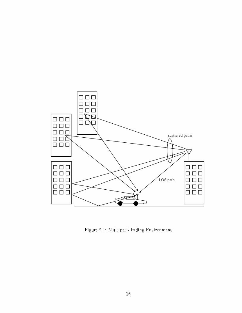
LOS path
scattered paths
Figure 2.1: Multipath Fading Environment
16

With regard to the impulse response h(� ; t), convolution is performed with respect
to the variable � , while dependence upon the variable t illustrates the time-varying
nature of the channel.
The fading exhibited by the multipath channel can be understood much more
clearly by considering the e�ects on an unmodulated carrier. This is accomplished
by setting u(t) = 1 for all values of t in equation (2.5), so that the received signal can
be expressed as
y(t) =Xi
ri(t) exp(j�i(t)) + n(t) (2.7)
where �i(t) = �2�fc�i(t). In this case, the received signal is just the sum of a number
of two-dimensional vectors, or phasors, having length ri(t) and phase �i(t) along
the ith path. The change in the attenuation ri(t) is not very signi�cant over short
periods of time; however, the phase �i(t) will change by 2� radians whenever the delay
�i(t) changes by f�1c , which is usually a very small number. It is assumed that the
attenuation and delay associated with di�erent paths are independent of each other.
The number of paths can usually be assumed to be large, so by applying the central
limit theorem, this sum of independent and identically distributed random processes
looks like a complex-valued Gaussian random process. This example illustrates the
reason why amplitude fading occurs. Since the received signal consists of the sum of a
large number of time-varying vectors, sometimes they add constructively causing an
increase in signal level, and sometimes they add destructively causing the amplitude
of the received signal to be very small. Since the attenuation factors ri(t) do not
change much over short periods of time, this fading phenomenon is mainly due to the
time variation of the phases �i(t).
In order to illustrate the dispersive e�ects of the channel, the auto-correlation
of the channel impulse response h(� ; t) shown in (2.6) is examined. The response
is modelled as a complex-valued Gaussian random process, so the auto-correlation
function is
Rh(�1; �2; t1; t2) =1
2E fh(�1; t1)h�(�2; t2)g : (2.8)
It is assumed that the random process is wide sense stationary so that the auto-
correlation depends only on the time di�erence �t = t2 � t1. It is also assumed
that the scattering is uncorrelated, which means that the attenuation and phase
17
shifts associated with di�erent path delays are uncorrelated. This means that the
expression in (2.8) will equal zero unless �1 = �2. Incorporating these assumptions
into equation (2.8) results in the auto-correlation function being expressed in the form
Rh(� ; �t), where the parameter � is equal to both �1 and �2. By letting �t = 0, the
multipath intensity pro�le Rh(�) is obtained. This is the average power output of the
channel as a function of the delay � . Let Tm be the range of � over which Rh(�) is
essentially non-zero. The parameter Tm is called the multipath spread of the channel,
and is the average length of time over which the energy of a very narrow pulse, or
impulse, is dispersed. If Tm happens to be larger than the signalling interval T , then
the energy of the transmitted symbol will be dispersed over other signalling intervals
causing intersymbol interference to appear in the received waveform.
An alternate approach to investigating the e�ects of time dispersion is to �nd the
auto-correlation of the channel transfer function H(f ; t), which is just the Fourier
transform of h(� ; t) taken with respect to the variable � . By using the same assump-
tions that were used to simplify equation (2.8), the auto-correlation function obtained
is
RH(f1; f2; t1; t2) =1
2E fH(f1; t1)H
�(f2; t2)g (2.9)
or equivalently RH(�f ; �t), where �f = f2� f1 is the di�erence in frequency. Once
again by letting �t = 0, the resulting auto-correlation function is denoted as RH(�f).
De�ne (�f)H to be the range of frequencies over which RH(�f) is essentially non-
zero. This is called the coherence bandwidth of the channel, and can be estimated as
(�f)H � T�1m . Depending on the frequency spectrum of the signal, the channel can
be classi�ed as belonging to one of two categories. If (�f)H is large in comparison
with the bandwidth of the transmitted signal, then the spectrum of the signal is not
a�ected. In this case the channel is called at fading or frequency non-selective. If
(�f)H is small in comparison to the bandwidth of the transmitted signal, then the
spectrum of the signal will be altered by the channel transfer function, resulting in a
distortion of the waveform. The received signal may exhibit the e�ects of intersymbol
interference due to this distortion. In this case, the channel is called frequency-
selective.
Since the mobile unit is usually in motion, the lengths of the propagation paths
18

are constantly changing, and this results in frequency dispersion of the transmitted
signal. Taking the Fourier transform of the auto-correlation function Rh(� ; �t) with
respect to �t and integrating over � , the power spectral density function obtained is
Sh(fD) =Z 1
�1
Z 1
�1Rh(� ; �t) exp(�j2�fD�t)d�td�: (2.10)
This is called the Doppler power spectrum of the channel, and the parameter fD is
called the Doppler frequency. Thus, the time variation of the channel results in a
Doppler spreading of the signal spectrum as well as a possible spectral shift. Let BD
be the set of fD over which Sh(fD) is essentially non-zero. This number is called
the Doppler spread of the channel, and indicates the range of frequency over which
the energy in a transmitted signal may be dispersed. The coherence time of the
channel is de�ned as (�t)h � B�1D , and measures the length of time over which the
fading process is considered to be correlated. A channel with a large BD has a small
coherence time and is called fast fading, since the channel response varies quickly
with time. A slow fading channel will have a large coherence time and experience
fades of longer duration.
For a signal with wavelength � which arrives at an angle with respect to the
direction of a vehicle travelling at a velocity v, the Doppler frequency is
fD =v
�cos : (2.11)
Frequency dispersion is detrimental to practical communication systems, so in anal-
ysis, the largest possible Doppler frequency is often used to represent the worst case.
The maximum Doppler frequency is simply
fDmax =����v����� : (2.12)
This model of a multipath fading channel is based on a physical interpretation
of the transmission medium, and while very general, can usually be simpli�ed when
analyzing a particular communication system. This requires additional assumptions
which depend on the particular system. A number of speci�c amplitude fading models
are presented next for non-dispersive channels, and can be augmented to include the
e�ects of both frequency and time dispersion.
19

2.2 Amplitude Fading Models
In order to focus on amplitude fading, non-dispersive channels are considered here.
Although no channel will be completely free of dispersion, sometimes the amount is
so small and the e�ects so negligible that the assumption of no dispersion is valid.
When no time dispersion is present, the channel will be at fading and the received
signal will not be distorted. When frequency dispersion is relatively insigni�cant, the
channel is described as slow fading, because variation of the fading process is limited
by the Doppler power spectrum. Since the random fading process �(t) changes very
slowly, it can be represented as a random variable � over any given signalling interval.
Using this assumption with a particular value � of the fading variable �1, the received
signal over a short period of time can be expressed in the form
y(t) = �u(t) + n(t): (2.13)
As was indicated in the previous section, the e�ect of fading is modelled as a complex-
valued Gaussian variate � with mean m� and variance �2�. The probability density
function (pdf) for this distribution is
p�(�) =1
2��2�exp
�j� �m�j2
2�2�
!: (2.14)
Due to the slow variation of the channel, it is sometimes assumed that the phase
can be tracked perfectly in the receiver after fading occurs. Since � is a complex-
valued Gaussian random variable, the phase � = arg � will be modelled as a uniform
random variable � with pdf
p�(�) =
8><>:
12�
�� < � � �
0 otherwise: (2.15)
The statistical distribution of the envelope r, which is the magnitude of �, takes
on di�erent forms depending on the particular fading scenario. In some cases it is
desirable to focus on the fading amplitude separately from the phase, since processes
in the receiver such as equalization or diversity combining operate on the complex
1 Random variables are indicated by uppercase symbols, whereas a particular value of the randomvariable is represented by the corresponding lower case symbol. The same convention is used herefor random processes.
20

envelope of the received signal after fading e�ects on the phase have been corrected.
Various statistical models for amplitude fading are described next.
2.2.1 Rayleigh Fading
In urban areas, a mobile unit is usually surrounded by many large buildings as well
as other vehicles. In this case it is unlikely that a LOS path exists, and the received
signal consists only of scattered components. With no LOS path, the complex-valued
Gaussian fading variable will have a zero mean. Let r = j�j be the envelope of thefading variable. By setting m� = 0 and performing a change of variables in equation
(2.14), the pdf of the random envelope R is derived to be
pR(r) =r
�2�exp
� r2
2�2�
!for r � 0 (2.16)
where it is understood here, and throughout the thesis, that any pdf such as pR(r)
which is de�ned for r � 0 takes on a value of zero for r < 0. This is called the Rayleigh
distribution, and usually represents the most severe case of amplitude fading. When
performing analysis, it is sometimes convenient to set EfR2g = 1 so that the average
power attenuation is unity. This is possible since the actual average loss due to long
term fading and free-space attenuation can be factored out, and the performance
of a communication system can be studied in the context of a short term fading
environment [34, pp. 169-171]. Usually messages are short in comparison to variations
in long term fading, so it is the short term models that are of interest. To set the
average power attenuation to unity, let �2� = 12in the pdf given by equation (2.16).
The resulting form of the Rayleigh density is
pR(r) = 2r exp��r2
�for r � 0: (2.17)
Since Rayleigh fading usually represents the worst case of fading, it has been used
as a basis for a number of fading channel studies [21, 35]. Also, the Rayleigh pdf
is simpler to manipulate mathematically than those describing other fading models,
which makes it favorable for use in analysis.
21

2.2.2 Rician Fading
In residential and rural areas, the lack of large surrounding structures allows for a
LOS component to exist in the received signal. In this case, the complex-valued
Gaussian fading process no longer has a zero mean. Let � = jm�j, where m� is the
mean value of �. By letting r = j�j and performing a change of variables in equation
(2.14), the envelope of the fading variable R will have the probability density
pR(r) =r
�2�exp
�r
2 + �2
2�2�
!I0
r�
�2�
!for r � 0 (2.18)
where I0(�) is the modi�ed Bessel function of the �rst kind and of zero order [16]. In
this case, the fading envelope is said to have a Rician distribution. The ratio of the
power in the LOS component to that in the scattered components is called the Rician
channel parameter, and is determined by the relation
R =�2
2�2�: (2.19)
When R = 0 there is no power in the LOS component, and the model reduces to
that of a Rayleigh channel. When R = 1, all the power is in the LOS component
and no scattered components exist, so the model looks like a simple AWGN channel.
In order to set EfR2g = 1, as was done for the Rayleigh channel, it is required that
�2 + 2�2� = 1. This is obtained by setting �2 = R1+ R
and 2�2� = 11+ R
in equation
(2.18). The resulting form of the Rician pdf is
pR(r) = 2r(1+ R) exp��r2(1 + R)� R
�I0
�2rq R(1 + R)
�for r � 0: (2.20)
The Rician fading model has been used in studies of mobile satellite communication
in the United States [16].
2.2.3 Shadowed Rician Fading
In some cases the LOS component of the received signal is not constant, but is prone
to shadowing e�ects from foliage, buildings, or uneven terrain. In this case, the
magnitude of the LOS component is assumed to be a random variable Z, described
by a lognormal distribution with pdf
pZ(�) =1
�q2��2Z
exp
�(ln � �mZ)
2
2�2Z
!for � > 0: (2.21)
22

Conditioned on the �xed value of Z = �, the fading amplitude will have a Rician
density as shown in equation (2.18). To incorporate the e�ects of shadowing, it is
required that the Rician pdf be averaged over the distribution of Z. The resulting
pdf for this channel can be expressed in the form
pR(r) =r
�2�
1q2��2Z
Z 1
0
1
�exp
�(ln � �mZ)
2
2�2Z� (r2 + �2)
2�2�
!I0
r�
�2�
!d� for r � 0
(2.22)
which is obtained by averaging equation (2.18) over the pdf given in (2.21). Loo has
shown that this model �ts the experimental data measured for the Canadian land
mobile satellite channel. In [36] he presents values for �2Z , mZ , and �2� which were
obtained from experimental measurements, and that correspond to di�erent degrees
of shadowing.
2.2.4 Nakagami Fading
The Nakagami fading model, described by the Nakagami-m distribution, is an approx-
imation that links two di�erent fading distributions. The �rst is the Rician fading
model, which is also known as the Nakagami-n distribution, and spans the range from
Rayleigh fading to the AWGN channel. It was stated that the Rician distribution de-
scribes the envelope of a complex-valued Gaussian random variable with components
that are uncorrelated and have equal variance as well as non-zero mean values. This
is a chi distribution with two degrees of freedom [37]. The other distribution that is
included in the Nakagami model is known as the Nakagami-q distribution, and spans
the range from one-sided Gaussian fading to Rayleigh fading. The q-distribution de-
scribes the envelope of a complex-valued Gaussian random variable with uncorrelated
components that have unequal variance and a mean value of zero. The q-distribution
describes fading that is even more severe than the Rayleigh channel. The Nakagami
model approximates both of these distributions with the pdf
pR(r) =2mmr2m�1
�(m)mexp
��mr2�
for r � 0 (2.23)
where m is the Nakagami channel parameter, is equal to the second moment of
R, and �(�) is the well known gamma function or generalized factorial. Crepeau [38]
23

describes the Nakagami distribution as a central chi distribution generalized to a non-
integral number of degrees of freedom. When m = 12the model describes one-sided
Gaussian fading, which is the case where only one faded component of the complex-
valued signal is available at the output of the channel. When m = 1 the Rayleigh
model is obtained, and when m = 1 the channel is non-fading. Unfortunately,
this model is not as intuitive on a physical basis as the Rician model and has no
accompanying phase distribution. However, this model is gaining popularity, since
in many cases it matches measured data better than the Rician model [39, 40]. The
pdf for the Nakagami model is also easier to use in mathematical analysis than the
Rician pdf. To set the average power attenuation to unity in this model, let = 1,
which results in the modi�ed pdf
pR(r) =2mmr2m�1
�(m)exp
��mr2
�for r � 0: (2.24)
2.3 E�ects of Frequency Dispersion
The amplitude fading models presented in the previous section remain valid for a at
fading channel even if the amount of frequency dispersion due to the channel increases.
For the digital cellular phone system proposed in North America, carrier frequencies
will be in the 900 MHz frequency band. If vehicle speeds from 0 to 100 mph are
considered, then from equation (2.12), resulting Doppler frequencies can range from
approximately 0 to 130 Hz. This is still very small compared to the signal bandwidth
of 30 kHz. So for most cases of interest, the fading amplitude will remain essentially
constant over a symbol interval. The e�ects of frequency dispersion in uence the
practical design of a communication system, which in turn a�ects the models that
are used to describe the channel. The practical considerations examined here are
symbol interleaving, diversity combining, and channel state estimation.
2.3.1 Symbol Interleaving
When a fade of long duration occurs during transmission, a sequence of symbols
are made susceptible to additive noise, resulting in a corresponding long burst of
errors. In order to break up bursts of errors, interleaving is often used. Interleaving
24
can be performed either on channel symbols or on individual bits. Although bit
interleaving is more e�ective in making bit errors appear random, symbol interleaving
is more popular since it can make the channel appear e�ectively memoryless. The
performance of receivers, such as those that use the Viterbi algorithm, is improved
when the fading channel appears memoryless. Analysis is also simpli�ed, since a
joint probability density describing the channel could be factored into a product of
the marginal densities.
The simplest way to understand the e�ect of interleaving is to examine the opera-
tion of a block interleaver. In the transmitter, a block interleaver reads symbols into
a two-dimensional array by rows, and then transmits the symbols by columns. In the
receiver, a deinterleaver is used to put the symbols back in sequence. If a fade of long
duration were to occur, then the deinterleaved sequence would experience random
symbol errors rather than a long burst of errors. In reality, interleaving introduces
a delay which increases the time required for transmission. In some cases, such as
digital voice transmission, this delay must be kept minimal. The size of the inter-
leaver required is related to the coherence time of the channel. The column length of
a block interleaver should in fact be large enough so that the transmission time for a
column of symbols is at least one signalling interval longer than the coherence time
of the channel.
In [41], a convolutional interleaver is used in the study of mobile satellite channels.
A convolutional interleaver uses less memory elements than a block interleaver, but
the symbols are not equally separated. Wei [42] proposes that the interleaver be
matched to the coding scheme so that interleaving is more e�ective in a practical
communication system. This means that the same performance could be achieved
with a shorter interleaving delay. When performing analysis, it is common to assume
symbol interleaving is ideally in�nite. This assumption allows a memoryless channel
model to be used.
2.3.2 Diversity Combining
When a mobile unit comes to a stop, the time variation of the channel ceases. If
this should happen during the occurrence of a deep fade, then the channel would
25

e�ectively be lost until the mobile unit started moving again. In order to compensate
for such an occurrence, diversity is commonly used. Diversity may be obtained by
repeating transmission, as in the case of time diversity, or by transmitting on di�erent
carriers, as in the case of frequency diversity. These types of diversity, however, do
not provide any bene�t when the mobile unit stops during the occurrence of a deep
fade. The bene�cial form to use in order to reduce the possibility of channel loss
is space diversity, which means that L di�erent antennae are used to receive the
signal. This method is also more eÆcient, since the same throughput and bandwidth
is used as a non-diversity system. If two antennae are separated by a distance d, then
the correlation coeÆcient between the Gaussian fading processes received by the two
antennae is given by [34]
�� = J0
2�d
�
!(2.25)
where J0(�) is a Bessel function of the �rst kind and of zero order, and � is the wave-
length of the signal. By spacing the antennae so that the minimum separation is 0:5�,
the fading processes received on any pair of antennae will be essentially uncorrelated2.
If one antenna were to receive a severely faded signal, it would be less likely that all
L would also be experiencing a deep fade at the same time. Thus, the probability
of losing the channel when the mobile unit is stationary is signi�cantly reduced. For
a 900 MHz carrier, � is approximately 13 inches. So a case of practical interest for
the digital cellular phone system would be the use of two antennae separated by a
distance of approximately 6-7 inches.
After adjusting the received signals over each antenna so that they are cophased,
the receiver combines them to obtain
y(t) =LXi=1
aiyi(t) (2.26)
where the ai are weighting factors, and yi(t) is the complex envelope of the received
signal for the ith antenna. Maximal-ratio combining sets the ai so that the carrier-to-
noise ratio is maximized. This is achieved when ai =rini, where ri is the envelope of
2 When results are obtained for systems with antenna diversity, the correlation coeÆcient usuallyappears in the form j��j2. Although �� 6= 0 when d = 0:5�, the value of j��j2 is suÆciently negligibleat this point, and the fading processes are considered to be essentially uncorrelated from a practicalviewpoint.
26

the fading process experienced by the ith antenna, and ni is the additive noise which
corrupts the signal received by the ith antenna. Although this technique is optimum,
it requires additional complexity in order to estimate the weighting factors ai, as the
ri cannot be directly obtained at the receiver. Equal-gain (i.e. constant ai) combining
is slightly worse in performance, but can be implemented with an inexpensive phase-
locked summing circuit [43]. After adjusting the phases for each antenna, the receiver
simply adds together the complex envelopes of the received signals. In this case, ai = 1
for all i in equation (2.26). Selective diversity combining is the simplest technique to
implement, but has the worst performance. This technique merely selects the best
signal from all L antennae. With regard to equation (2.26), if the jth path has the
strongest carrier-to-noise ratio, then aj = 1, and ai = 0 for all the other paths.
2.3.3 Channel State Estimation
In order to transmit information reliably over a fading channel when using uncoded
modulation or a technique such as TCM, some information must be obtained about
the fading variable �. In coding research, it is usually assumed that some information
about � is given without any mention of how this information is obtained. Divsalar
and Simon [16] assumed two di�erent cases for channel state information (CSI). In the
case of ideal CSI, the receiver is assumed to know the fading variable completely. For
a slow fading channel, it is reasonable to assume that a fairly good channel estimate
can be obtained. The other extreme case was termed no CSI. This means that there
is no information about the fading envelope, but it is assumed that the phase of the
fading process can be tracked. In this case, knowledge of the phase constitutes the
CSI.
If the fading is modelled as a complex-valued Gaussian random process, then
the actual fading variable � and the estimate ~� can be modelled as being jointly
Gaussian. It is assumed that the mean value of these variables are equal, and that
the correlation coeÆcient � is dependent upon the particular estimation scheme used.
The auto-correlation of the fading process is given by [34]
R�(�) = �2�J0 (2�fD�) (2.27)
27

where fD is the Doppler frequency. Any channel estimation scheme that involves a
time delay between the occurrence of � and the availability of ~� will yield a correlation
coeÆcient that is dependent upon the amount of frequency dispersion.
One practical channel estimation scheme involves the transmission of a pilot tone
along with the data signal. Since this tone is always known, the fading variable can
be determined by observing the amplitude and phase of the tone at the receiver.
The spectrum of the data signal should contain a spectral null in order to facilitate
extraction of the tone. The channel estimator consists of a bandpass pilot extraction
�lter in the receiver with bandwidth Wp. The bandwidth must be large enough to
pass the fading process without distortion, so it is assumed that Wp � 2BD. In [35],
it is stated that the squared magnitude of the correlation coeÆcient is
j�j2 = 1
1 +�1+
�(WpT )
��EsN0
��1 (2.28)
where is the ratio of the energy in the pilot tone to that in the data signal, T is the
duration of a signalling interval, and �Es represents the total average received symbol
energy in both the data and the pilot tone. By examining this expression, it is evident
that the quality of the channel estimate is dependent upon the SNR as well as the
Doppler spread.
Di�erential phase shift keying is a desirable type of modulation in environments
where phase estimation is diÆcult. If channel symbols xi are modelled as complex
numbers with unit magnitude, the di�erential encoding process can be described by
the complex multiplication xi = xi�1xi, where xi is the di�erentially encoded channel
symbol transmitted at time i. Transmission of the phase di�erences results in the
received symbol
yi = �ixi + ni = �ixi�1xi + ni: (2.29)
A noisy estimate of �xi�1 may be obtained by using ~�i = �i�1xi�1 + ni�1, which
is simply the channel symbol received during the previous signalling interval. The
resulting correlation coeÆcient has squared magnitude [35]
j�j2 = J20 (2�fDT )
1 +�
�EsN0
��1 : (2.30)
28
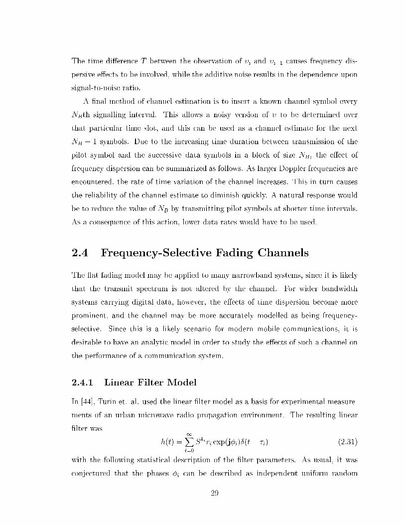
The time di�erence T between the observation of �i and �i�1 causes frequency dis-
persive e�ects to be involved, while the additive noise results in the dependence upon
signal-to-noise ratio.
A �nal method of channel estimation is to insert a known channel symbol every
NBth signalling interval. This allows a noisy version of � to be determined over
that particular time slot, and this can be used as a channel estimate for the next
NB � 1 symbols. Due to the increasing time duration between transmission of the
pilot symbol and the successive data symbols in a block of size NB, the e�ect of
frequency dispersion can be summarized as follows. As larger Doppler frequencies are
encountered, the rate of time variation of the channel increases. This in turn causes
the reliability of the channel estimate to diminish quickly. A natural response would
be to reduce the value of NB by transmitting pilot symbols at shorter time intervals.
As a consequence of this action, lower data rates would have to be used.
2.4 Frequency-Selective Fading Channels
The at fading model may be applied to many narrowband systems, since it is likely
that the transmit spectrum is not altered by the channel. For wider bandwidth
systems carrying digital data, however, the e�ects of time dispersion become more
prominent, and the channel may be more accurately modelled as being frequency-
selective. Since this is a likely scenario for modern mobile communications, it is
desirable to have an analytic model in order to study the e�ects of such a channel on
the performance of a communication system.
2.4.1 Linear Filter Model
In [44], Turin et. al. used the linear �lter model as a basis for experimental measure-
ments of an urban microwave radio propagation environment. The resulting linear
�lter was
h(t) =1Xi=0
Skiri exp(j�i)Æ(t� �i) (2.31)
with the following statistical description of the �lter parameters. As usual, it was
conjectured that the phases �i can be described as independent uniform random
29
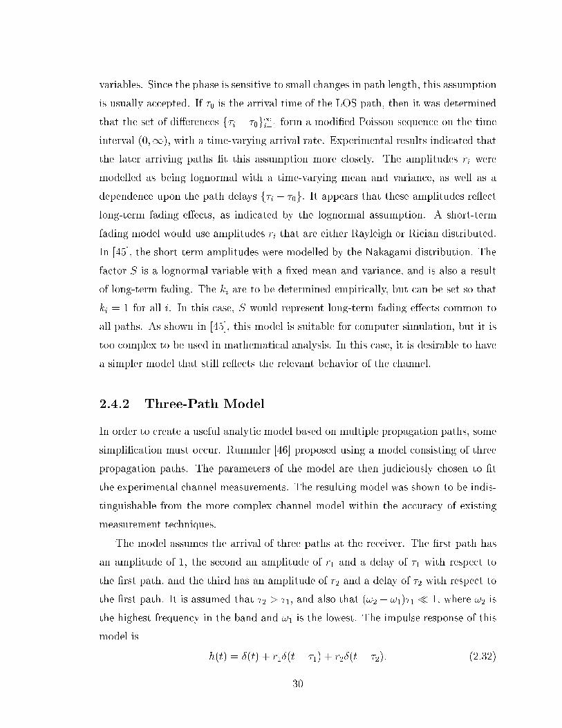
variables. Since the phase is sensitive to small changes in path length, this assumption
is usually accepted. If �0 is the arrival time of the LOS path, then it was determined
that the set of di�erences f�i � �0g1i=1 form a modi�ed Poisson sequence on the time
interval (0;1), with a time-varying arrival rate. Experimental results indicated that
the later arriving paths �t this assumption more closely. The amplitudes ri were
modelled as being lognormal with a time-varying mean and variance, as well as a
dependence upon the path delays f�i � �0g. It appears that these amplitudes re ect
long-term fading e�ects, as indicated by the lognormal assumption. A short-term
fading model would use amplitudes ri that are either Rayleigh or Rician distributed.
In [45], the short-term amplitudes were modelled by the Nakagami distribution. The
factor S is a lognormal variable with a �xed mean and variance, and is also a result
of long-term fading. The ki are to be determined empirically, but can be set so that
ki = 1 for all i. In this case, S would represent long-term fading e�ects common to
all paths. As shown in [45], this model is suitable for computer simulation, but it is
too complex to be used in mathematical analysis. In this case, it is desirable to have
a simpler model that still re ects the relevant behavior of the channel.
2.4.2 Three-Path Model
In order to create a useful analytic model based on multiple propagation paths, some
simpli�cation must occur. Rummler [46] proposed using a model consisting of three
propagation paths. The parameters of the model are then judiciously chosen to �t
the experimental channel measurements. The resulting model was shown to be indis-
tinguishable from the more complex channel model within the accuracy of existing
measurement techniques.
The model assumes the arrival of three paths at the receiver. The �rst path has
an amplitude of 1, the second an amplitude of r1 and a delay of �1 with respect to
the �rst path, and the third has an amplitude of r2 and a delay of �2 with respect to
the �rst path. It is assumed that �2 > �1, and also that (!2 � !1)�1 � 1, where !2 is
the highest frequency in the band and !1 is the lowest. The impulse response of this
model is
h(t) = Æ(t) + r1Æ(t� �1) + r2Æ(t� �2): (2.32)
30

By applying the Fourier transform to h(t), the transfer function of the channel is
determined to be
H(!) = 1 + r1 exp(�j!�1) + r2 exp(�j!�2): (2.33)
The vector that results from summing the �rst two components of H(!) will have
amplitude a and phase �. Since the value of �1 is assumed to be very small, the term
!�1 can be considered to be essentially constant for all ! in the frequency band, which
allows the value of � to be treated as being constant. If !0 is the radian frequency
at which H(!) takes on its minimum value, then this will occur when the third term
in (2.33) opposes the sum of the �rst two, or in other words when � = !0�2 � �. By
setting r2 = ab, the transfer characteristic becomes
H(!) = a exp(�j(!0�2 � �)) + ab exp(�j!�2): (2.34)
Finally, by rotating H(!) through an angle � = !0�2 � � and setting �2 = � , the
transfer function is expressed in the form
H(!) = a [1� b exp (�j (! � !0) �)] : (2.35)
A plot of H(!) taken from [46] is shown in Figure 2.2. The parameter a is called
the scale parameter, and sets the overall gain of H(!). The variable b is called the
shape parameter, and controls the shape of H(!) as well as the depth of the notches.
In Figure 2.2, the notch depth is 20 log�1+b1�b�. The spacing between the minima of
H(!) is ��1, where � is the delay di�erence of the channel. By changing the various
parameters of H(!), one can see that notches can be included at a number of fre-
quencies within the transmit spectrum. For notches located out of band, a variety
of slopes can be obtained. It was stated in [46] that the path parameters overspecify
the channel. That is, within the accuracy of available measurement techniques, the
parameters are not unique for a given transfer characteristic. In order to specify a
unique model, it is required that one of the parameters a, b, �, or � , be �xed. Although
�xing the delay di�erence � does not intuitively seem reasonable, doing so results in
the most e�ective model. The value of � can be set to Tm, the multipath spread of
the channel. The remaining parameters must be given a statistical characterization.
31

35
30
25
20
15
-20l
og|H
(f)|
-50 0 50 100 150 200 250
f - fo (MHz)
Figure 2.2: Channel Transfer Function of the Three-Path Model
32

In [46], the model was used to describe a microwave radio channel. The scale pa-
rameter a was modelled as being lognormal conditioned on b, which indicates that
long-term fading e�ects are included. The shape parameter was given a distribution
of the form (1� b)2:3, and !0 was distributed uniformly at two levels. Unfortunately,
statistics that would describe a mobile fading channel have not been determined using
this model. However, by using this model as a basis and making some assumptions
based on an interpretation of the physical e�ects of Rayleigh fading, a simple model
for a frequency-selective mobile channel is obtained.
2.4.3 Two-Path Rayleigh Model
The two-path Rayleigh model is used to model frequency-selective e�ects on mobile
channels [47, 48]. Justi�cation for the use of this model is based on the close �t of the
simple three-path model to fading channels, as well as the lack of a LOS component in
many mobile channels. The two-path model can be derived similarly to the three-path
model by removing the LOS path. This results in the channel impulse response
h(t) = �1Æ(t� �1) + �2Æ(t� �2) (2.36)
where �1 and �2 are modelled as independent complex-valued Gaussian fading vari-
ables with zero mean. It may be assumed that the variances of the random variables
�1 and �2 are �2�1
= 12(1+ )
and �2�2=
2(1+ ), respectively. This ensures that the sum
of the two fading processes has a unity gain. The delays are set so that �1 = 0 and
�2 = � , where once again � is the delay di�erence of the channel.
When a channel is at fading, the e�ect of fading on the signal can be resolved
into a scaling of the amplitude of the transmitted symbol in addition to a phase
rotation. In this case, analysis can be performed in terms of the channel symbols and
without regard to the baseband pulse used. When the channel is frequency-selective,
intersymbol interference occurs in the received signal and the baseband pulse can no
longer be ignored. In this case the baseband signal is expressed in the form
u(t) =Xi
xig(t� iT ) (2.37)
where xi is the channel symbol transmitted during the ith signalling interval, and g(t)
33

is the baseband pulse used. The shape and duration of g(t) has a signi�cant e�ect on
communication over frequency-selective fading channels.
A number of models have been presented, which are used to represent the e�ect
that mobile communication channels have on signals. These models can also be
used as a basis for determining the limits that multipath fading channels impose on
communication.
34

Chapter 3
Information Theoretic Bounds for Ideal
Fading Channels
In this chapter, results from the �eld of information theory are utilized in order to
determine the fundamental limits of communication over multipath fading channels.
Channel capacity and average mutual information are two upper bounds on trans-
mission rate which are used to determine the losses incurred due to fading. In order
to isolate the e�ects of fading from other factors, such as time dispersion and Doppler
spread, an idealized channel model is used. This idealized model is the same one that
is generally used in channel coding research. The limits obtained here can also be
used as a benchmark for code performance. This eliminates the necessity of having to
use the performance of other known codes, or the AWGN channel performance of the
code in question, as a basis for judging its merit. Constraints on both average and
peak power are considered. Physical restrictions on the size of mobile transmitters
place a limit on the peak power available, and it is this constraint which is presumably
more relevant to mobile communications. Also related to peak power performance is
the peak-to-average power ratio of the constellation. This number gives an indication
of the e�ect of signal dependent perturbations, such as non-linear distortion, on the
performance of the system. In order to reduce the possibility of channel loss, multiple
antennae are often used in mobile systems. The e�ect of this space diversity on com-
munication rate is examined from an information theoretic viewpoint. Finally, the
gains possible through the use of shaping and channel coding are determined through
comparison of channel capacity with the performance of uncoded modulation.
35

3.1 Information Theoretic Concepts
Average mutual information and channel capacity are two information theoretic
bounds on the maximum communication rate over a channel. The rate is a max-
imum in the sense that if it is exceeded, then the probability of a detection error
occurring in the receiver cannot be made arbitrarily small. Some of the key de�-
nitions required from the �eld of information theory are stated here along with the
channel coding theorem. More detail can be found in texts by Gallager [27] or Cover
and Thomas [49].
In order to simplify notation, the probability density function of a random variable
X will be denoted by p(x) rather than using a form such as pX(x). The symbol x
serves here both as a label for the random variable X, as well as an argument for
the pdf. The pdf's p(x) and p(y) are not to be considered the same unless indicated.
This notation is assumed from now on for all probability densities and probability
mass functions. In addition, although the following de�nitions are stated in terms
of probability density functions, the obvious extensions to discrete distributions and
probability mass functions will be assumed to be understood.
A mathematical de�nition of a general communication channel is required in order
to interpret information theoretic results in a communications context.
De�nition 3.1 A communication channel is de�ned to consist of an input alphabet
X , an output alphabet Y, and a transition probability assignment p(yjx). The input
and output alphabets can be either discrete-valued or continuous-valued.
A case of practical interest is when X is a discrete-valued alphabet, such as a signal
constellation, and Y is continuous-valued, representing the set of all possible corrupted
channel outputs. The transition probabilities p(yjx) will depend on the channel model
used. For the fading channel models presented in the previous chapter, additional
information is available at the output of the channel in the form of the estimate ~�
of the fading variable �. Since it is desirable to use this additional information in
determining which symbol was transmitted, the transition probabilities for fading
channels will be of the form p(yjx; ~�).The entropy of a random variable X can be interpreted as a measure of the
36

uncertainty in determining the value of X, or equivalently, as the average amount of
information it contains.
De�nition 3.2 If the random variable X has a pdf p(x), then the entropy H(X) is
de�ned as
H(X) = �Ep(x) flog p(x)g (3.1)
where Ep(x) denotes expectation taken over p(x).
This de�nition assumes that both the pdf p(x) as well as the average value of log p(x)
exist, which is likely for cases of practical interest. For a discrete-valued random
variable, the entropy is always positive and absolute. For a continuous-valued random
variable, however, the entropy is taken relative to the coordinate system used and may
take on negative values. When X is a continuous-valued random variable, H(X) is
sometimes referred to as di�erential entropy. Usually the logarithm used is assumed
to have base 2, which causes the entropy to be measured in units of bits. Entropy
can also be de�ned for a set of random variables.
De�nition 3.3 If a set of random variables X = (X1; : : : ; Xn) are speci�ed by a
joint pdf p(x1; : : : ; xn), then the joint entropy of the set is de�ned as
H(X) = �Ep(x1;:::;xn) flog p(x1; : : : ; xn)g (3.2)
where Ep(x1;:::;xn) denotes expectation taken over p(x1; : : : ; xn).
Sometimes knowledge of one random variable a�ects the uncertainty associated
with another random variable. In this case, the entropy can be conditioned on the
known variable.
De�nition 3.4 If random variables X and Y have a joint pdf p(x; y), then the con-
ditional entropy of X given knowledge of Y is de�ned as
H(XjY ) = �Ep(x;y) flog p(xjy)g (3.3)
where Ep(x;y) denotes expectation taken over p(x; y).
37

Conditioning can only reduce entropy, and H(XjY ) is always less than or equal to
H(X) [49, p. 27]. The case where equality holds is when the random variables are
statistically independent. Conditional entropy can also be expanded to sets of random
variables, resulting in a conditional joint entropy. For example, the joint entropy of
the set X = (X1; : : : ; Xn) given knowledge of the set Y = (Y1; : : : ; Ym) is
H(XjY ) = �Ep(x1;:::;xn;y1;:::;ym) flog p(x1; : : : ; xnjy1; : : : ; ym)g (3.4)
where Ep(x1;:::;xn;y1;:::;ym) denotes expectation taken over the joint probability density
function p(x1; : : : ; xn; y1; : : : ; ym).
Average mutual information is a measure of the amount of information that two
random variables have in common.
De�nition 3.5 Suppose X and Y have a joint pdf p(x; y) and marginal pdf's p(x)
and p(y), respectively. The average mutual information (AMI) between X and Y is
de�ned as
I(X;Y ) = Ep(x;y)
(log
p(x; y)
p(x)p(y)
!)(3.5)
where Ep(x;y) denotes expectation taken over p(x; y).
By using Bayes' theorem and properties of the logarithm, equation (3.5) can be
rewritten in the form
I(X;Y ) = H(X)�H(XjY ): (3.6)
The conditional entropy H(XjY ) is commonly referred to as the equivocation of the
channel when X and Y represent the channel input and output, respectively. Average
mutual information can also be interpreted as the average reduction in uncertainty
of X given knowledge of the value of Y .
In the context of a communication system, the random channel output y is a
corrupted version of the transmitted symbol x, and must be used to determine the
value of x that was transmitted. For example, if the constellation X consists of 8
equally likely symbols, then the entropy H(X) of the input can be calculated to be
equal to log2 8 = 3 bits. If y is a good estimate of x, then the 3 bits of uncertainty
can essentially be eliminated. In other words, knowing the value of the variable Y
gives a good estimate of the variable X, and on average 3 bits/T can be transmitted
38

over the channel with a small probability of error. If y is not such a good estimate of
x, then knowledge of the value of Y does not reduce the uncertainty in the value of
X to such a great degree. In this case, less than 3 bits must be transmitted every T
seconds when using the constellation along with some coding scheme, otherwise the
number of errors occurring in the receiver cannot be controlled.
Notice from equation (3.5) that average mutual information is symmetric with
respect to the arguments. That is, I(X;Y ) = I(Y ;X), and knowledge of the random
variable X reduces the uncertainty in Y by the same amount as knowledge of Y re-
duces the uncertainty in X. This symmetry results in an alternate form for expressing
average mutual information as a di�erence of entropies, and is given by the expression
I(X;Y ) = H(Y )�H(Y jX): (3.7)
Another fact of signi�cance is that for continuous-valued random variables, even
though the individual entropies may take on negative values, the average mutual
information is always positive and does not depend on the particular coordinate sys-
tem used [1].
Rather than being limited to single random variables, average mutual information
can also be de�ned between sets of random variables. For instance, the AMI between
the sets of random variables X = (X1; : : : ; Xn) and Y = (Y1; : : : ; Ym) is de�ned by
the equation
I(X;Y ) = Ep(x1;:::;xn;y1;:::;ym)
(log
p(x1; : : : ; xn; y1; : : : ; ym)
p(x1; : : : ; xn)p(y1; : : : ; ym)
!)(3.8)
which is just an extension of equation (3.5). Also, the AMI between two sets of random
variables can be conditioned on another set of known random variables. For example,
the conditional average mutual information between the sets of random variables
X = (X1; : : : ; Xn) and Y = (Y1; : : : ; Ym) given knowledge of the set Z = (Z1; : : : ; Zl)
is
I(X;Y jZ) = E
(log
p(x1; : : : ; xn; y1; : : : ; ymjz1; : : : ; zl)
p(x1; : : : ; xnjz1; : : : ; zl)p(y1; : : : ; ymjz1; : : : ; zl)
!)(3.9)
where expectation is taken over the joint pdf p(x1; : : : ; xn; y1; : : : ; ym; z1; : : : ; zl).
Channel capacity is the ultimate limit for reliable transmission of data over a given
communication channel.
39

De�nition 3.6 The capacity C of a communication channel is de�ned as
C = maxp(x)
I(X;Y ) (3.10)
where maximization is taken over all possible distributions of the input alphabet.
Given a constraint on average transmitted power of the form EfjXj2g � Es, the
capacity of an AWGN channel is given by the well known equation [49, p. 242]
C = log2
�1 +
EsN0
�bits=T (3.11)
where N0 is the average power of the additive noise, and T is the time required
to transmit a channel symbol. The transmission medium here is represented as a
discrete-time channel, and the unit of bits/T is equivalent to bps/Hz1. If the channel
is ideal and has a bandwidth of W Hz, then the capacity can also be expressed in the
form
C = W log2
�1 +
EsN0
�bps: (3.12)
The capacity of the AWGN channel is achieved by using a continuous-valued input
alphabet that has a Gaussian distribution with zero mean and variance �2X = Es2.
This can be proven using the well-known result that given a constraint on average
power, a Gaussian distribution maximizes entropy [49, p. 234].
The importance of average mutual information and channel capacity can be sum-
marized by the channel coding theorem. This theorem states that as long as the
communication rate Rc is less than the channel capacity C, the probability of detec-
tion error Pr(e) can be made arbitrarily small by using long enough code sequences.
This can be stated more rigorously as follows.
Theorem 3.1 For every � > 0 and rate Rc < C, there exists a code consisting of
d2NBRce codewords of length NB, such that Pr(e) < �. Conversely, if there exists a
code consisting of d2NBRce codewords of length NB that results in Pr(e) ! 0, then
Rc < C.
1 Equivalence of the units of bits/T and bps/Hz is based on the assumption that no more thanW symbols per second can be transmitted in a bandwidth of W Hz [11].
40

For a proof of the theorem see [49, pp. 199-202]. If Rc < I(X;Y ) then Rc < C, so
for schemes using practical constellations with a given input probability assignment
p(x), the maximum communication rate can always be bounded from above by the
resulting average mutual information, and the channel coding theorem applies.
Ungerboeck [6] calculated AMI curves for the AWGN channel using practical
PSK and QAM constellations. For the AWGN channel, the received symbol can be
represented in the form y = x + n, where x is the transmitted symbol, and n is
the additive noise. The random noise variable N has a complex-valued Gaussian
distribution with zero mean and variance �2N . It is assumed that the symbol x comes
from a M -point constellation and has a uniform discrete probability mass function
(pmf) given by p(xi) =1M
for i = 1; : : : ;M . Given knowledge of the value X = xi,
the conditional pdf of the received symbol Y can be determined by performing a
translation of the noise variable N . The resulting pdf is
p(yjxi) = 1
2��2Nexp
�jy � xij2
2�2N
!: (3.13)
Given p(yjxi) and p(xi), the joint density p(xi; y) can be determined from the law of
total probability. The pdf's and pmf obtained can then be used in equation (3.5) to
obtain an expression for average mutual information in the form
I(X;Y ) = log2M � 1
M
MXi=1
Ep(n)
8<:log2
24 MXj=1
exp
�jxi � xj + nj2 � jnj2
2�2N
!359=; : (3.14)
Since a base 2 logarithm is used, the average mutual information has units of bits/T .
In equation (3.14), Ep(n) f�g denotes expectation taken over the pdf p(n) of the noise
variable N . This expression can be evaluated by means of a computer simulation.
What is meant by computer simulation is an evaluation of the statistical expectation
through Monte Carlo averaging of the enclosed expression. The reliability of those
results presented in the thesis which were obtained through computer simulation is
discussed in Appendix A.
Ungerboeck's AMI curves are shown in Figures 3.1 and 3.2 for PSK and QAM
constellations, respectively, along with the capacity curve for the AWGN channel.
The standard constellations considered in the thesis are the same as those used
in [6]. The term QAM is used here as a general label for the AMPM constellations
41
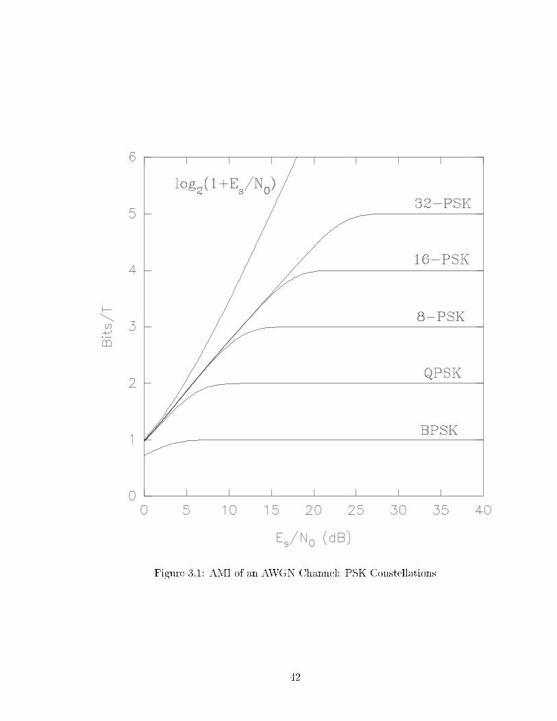
Figure 3.1: AMI of an AWGN Channel: PSK Constellations
42
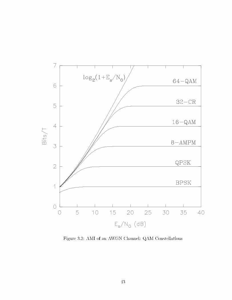
Figure 3.2: AMI of an AWGN Channel: QAM Constellations
43

considered in [6], which includes both square and cross-constellations, as well as the
8-AMPM signal set. Ungerboeck interpreted the AMI curves by observing that 2
bits/T can be transmitted with uncoded QPSK, obtaining an error probability of
10�5 when the SNR is 12.9 dB. However, by using an 8-PSK signal set, error-free
transmission of 2 bits/T is theoretically possible at a SNR of 5.8 dB. In addition, only
1 dB of further improvement can be obtained by reaching capacity. This is the basis
of Ungerboeck's heuristic design rule for trellis coding, which states that twice the
number of signal points as required for uncoded modulation can be used to obtain
most of the coding gain. The minimum values of SNR required to attain various
rates of AMI over an AWGN channel using standard PSK and QAM constellations
are contained in Tables 3.1 and 3.2, respectively. These results are used to determine
the losses incurred due to multipath fading.
3.2 Channels with Discrete-Valued Input
The same bounds used for the AWGN channel are implemented here in order to
determine the limits on reliable communication over fading channels when a discrete-
valued signal set is used. In this chapter, the fading channel is assumed to be ideal
in the sense characterized by the following de�nition.
De�nition 3.7 An ideal fading channel is one in which: i) The fading variables �
are known at the receiver. ii) The fading variables � are independent with respect to
time. iii) The transmitted pulse is not distorted or dispersed in time. iv) The fading
variables � remain essentially constant over an entire symbol interval.
An ideal fading channel satis�es those assumptions which are usually made in coding
research in order to simplify analysis. The �rst assumption is that the channel state
information is ideal. The second assumption indicates that ideally in�nite interleaving
is possible, which results in a memoryless channel model. The third assumption
means that the channel is at fading, and the �nal assumption indicates that the
channel is slow fading compared to the symbol rate. When this idealized model
is used, the in uence of time dispersion and Doppler spread are non-existent, and
this enables one to focus on the e�ects of amplitude fading alone. In general, if
44

Number of Signal Points
4 8 16 32
4.5 - - - 20.5 dB
4 - - - 17.4 dB
3.5 - - 14.6 dB 14.5 dB
AMI 3 - - 11.5 dB 11.5 dB
(Bits/T ) 2.5 - 8.8 dB 8.6 dB 8.6 dB
2 - 5.8 dB 5.8 dB 5.8 dB
1.5 3.4 dB 3.0 dB 3.0 dB 3.0 dB
1 0.2 dB 0.1 dB 0.1 dB 0.1 dB
Table 3.1: Minimum SNR Required for Various Rates of AMI on an AWGN Channel:
PSK Constellations
Number of Signal Points
4 8 16 32 64
5.5 - - - - 18.2 dB
5 - - - - 16.1 dB
4.5 - - - 14.8 dB 14.4 dB
4 - - - 12.7 dB 12.6 dB
AMI 3.5 - - 11.6 dB 10.8 dB 10.8 dB
(Bits/T ) 3 - - 9.3 dB 9.0 dB 9.0 dB
2.5 - 7.9 dB 7.2 dB 7.1 dB 7.1 dB
2 - 5.3 dB 5.1 dB 5.0 dB 5.0 dB
1.5 3.4 dB 2.9 dB 2.8 dB 2.7 dB 2.7 dB
1 0.2 dB 0.1 dB 0.1 dB 0.0 dB 0.0 dB
Table 3.2: Minimum SNR Required for Various Rates of AMI on an AWGN Channel:
QAM Constellations
45

any of these assumptions are not satis�ed, then it becomes more diÆcult to achieve
reliable communication over the channel. This is the reason that this fading model is
considered to be ideal.
The average mutual information for an ideal fading channel is derived here for
the case of when the input alphabet is a discrete-valued signal set and the output is
continuous-valued. Suppose there are M points in the discrete-valued signal constel-
lation with a priori probability p(xi). The entropy of the channel input is determined
from the expression
H(X) = �MXi=1
p(xi) log p(xi): (3.15)
At the output of the channel, both of the values y = �x+n and � are obtained. The
a posteriori probability that the particular value of X = xi was transmitted, given
knowledge of the variables Y and �, is determined by the pmf
p(xijy; �) = p(yjxi; �)p(xi)p(yj�) : (3.16)
The conditional entropy of the channel input given knowledge of the channel output
Y and the fading variable � is
H(XjY;�) =MXi=1
ZSY
ZS�p(y; xi; �) log
"p(yjxi; �)p(xi)
p(yj�)
#d�dy (3.17)
where SY and S� are the respective support sets for the variables Y and �. The
average mutual information can now be determined from the di�erence of entropies
I(X;Y j�) = H(X)�H(XjY;�): (3.18)
By factoring the joint pdf into p(y; xi; �) = p(yjxi; �)p(xi)p(�) and using the fact that
p(yj�) =PMj=1 p(yjxj; �)p(xj), the conditional entropy of the channel input given
knowledge of the channel output and fading variable can be expressed in the form
H(XjY;�) =MXi=1
ZSY
ZS�p(yjxi; �)p(xi)p(�) log
"p(yjxi; �)p(xi)PMj=1 p(yjxj; �)p(xj)
#d�dy: (3.19)
Assuming that the constellation has an equiprobable a priori distribution, the discrete
pmf of the input is p(xi) =1M
for i = 1; : : : ;M . Using this in equation (3.15) results
46

in H(X) = logM . Given knowledge of the variables X and �, the channel output
will have a statistical distribution described by the pdf
p(yjxi; �) = 1
2��2Nexp
�jy � �xij2
2�2N
!(3.20)
which is obtained from the pdf of the additive noise through translation of the variable
n. By substituting the required density and mass functions into equation (3.19), the
conditional entropy takes the form
H(XjY;�) = (3.21)
1
M
MXi=1
ZSY
ZS�p(yjxi; �)p(�) log
24 MXj=1
exp
�jy � �xjj2 � jy � �xij2
2�2N
!35 d�dy:
After making the substitution y = �xi + n into equation (3.21), averaging can be
performed over p(n) rather than p(yjxi; �). Using this fact, the average mutual infor-mation in bits/T can be expressed as
I(X;Y j�) = log2M � 1
M
MXi=1
Ep(n)p(�)
8<:log2
24 MXj=1
exp
�j�(xi � xj) + nj2 � jnj2
2�2N
!359=;
(3.22)
where Ep(n)p(�) denotes expectation taken over p(n)p(�). This statistical expectation
can be evaluated by means of computer simulation.
3.2.1 Standard Signal Constellations
The AMI is determined here for an ideal Rayleigh fading channel when standard
signal constellations are used as input to the channel. The average received symbol
energy is de�ned as �Es = Efj�Xj2g. When considering a signal constellation X , the
energy and power of a symbol x are usually assumed to both equal jxj2, and the terms
energy and power can then be interchanged. This may be based on the underlying
assumption that a matched �lter is used in the receiver, and that the pulse used to
transmit the symbol is assumed to be scaled so that the energy has a value of 1.
In order to evaluate equation (3.22), it is assumed that Efj�j2g = 1 and that the
constellation has been normalized so that EfjXj2g = 1. The SNR is then determined
by the value of �2N .
47

Figure 3.3 contains the AMI curves for when standard PSK constellations are
used as input to the channel, while Figure 3.4 illustrates the case for when QAM
constellations are used. In Rayleigh fading, the AMI curves do not rise as quickly
to a �nal value of log2M as in the AWGN case. Also, even when the average SNR
is as large as 40 dB, the average mutual information is still a little less than the �nal
value of log2M . This is re ected in the error performance of uncoded modulation.
In the case of an AWGN channel, bit error curves have a quickly decreasing waterfall
characteristic. Over fading channels, however, the error curves are almost linear and
decrease very slowly in comparison to noise channels. In [30] and [31], similar results
are presented in terms of the computational cuto� rate R0 of the channel. The cuto�
rate is a limit derived for the speci�c technique of sequential decoding, and must not
be surpassed in order to ensure that the average computational load remains �nite.
Since other known decoding techniques also become impractical at rates above R0, it
has been touted for some time as being a practical limit on the rate of reliable data
transmission. Due to the transitory nature of the term `practical' when applied to
communications technology, it is preferable to determine the ultimate limit without
regard to any speci�c decoding technique.
The minimum values of average SNR required to attain various rates of AMI are
shown in Table 3.3 for PSK signal sets and in Table 3.4 for QAM. When using coded
modulation, less than log2M bits/T are transmitted with a constellation consisting
ofM symbols, so it is of interest to look at the loss due to fading for lower data rates.
Table 3.5 compares the loss in SNR due to multipath fading when PSK constellations
are used as input to the channel. Similar results for QAM constellations are shown
in Table 3.6. This loss is the di�erence in SNR where theoretically error-free trans-
mission is possible at the given data rate. For example, the AMI curve for 16-QAM
indicates that error free transmission at a rate of 3 bits/T is possible for an average
SNR greater than or equal to 12.3 dB, whereas a SNR of 9.3 dB is required on the
AWGN channel. Thus, when using a 16-QAM constellation, the loss due to fading at
a rate of 3 bits/T is 3.0 dB.
In order to interpret the results presented, �rst consider constellations which are
equal in size and have comparable values of AMI. When considering transmission over
48

Figure 3.3: AMI of an Ideal Rayleigh Fading Channel: PSK Constellations
49

Figure 3.4: AMI of an Ideal Rayleigh Fading Channel: QAM Constellations
50

Number of Signal Points
4 8 16 32
4.5 - - - 24.6 dB
4 - - - 20.3 dB
3.5 - - 18.6 dB 17.0 dB
AMI 3 - - 14.4 dB 14.0 dB
(Bits/T ) 2.5 - 12.7 dB 11.1 dB 11.0 dB
2 - 8.4 dB 8.0 dB 8.0 dB
1.5 6.7 dB 4.9 dB 4.9 dB 4.9 dB
1 1.8 dB 1.4 dB 1.4 dB 1.4 dB
Table 3.3: Minimum SNR Required for Various Rates of AMI on an Ideal Rayleigh
Fading Channel: PSK Constellations
Number of Signal Points
4 8 16 32 64
5.5 - - - - 23.4 dB
5 - - - - 19.7 dB
4.5 - - - 19.8 dB 17.2 dB
4 - - - 16.1 dB 15.0 dB
AMI 3.5 - - 16.2 dB 13.4 dB 13.0 dB
(Bits/T ) 3 - - 12.3 dB 11.1 dB 11.0 dB
2.5 - 12.1 dB 9.5 dB 9.0 dB 8.9 dB
2 - 7.9 dB 6.9 dB 6.7 dB 6.7 dB
1.5 6.7 dB 4.6 dB 4.3 dB 4.2 dB 4.2 dB
1 1.8 dB 1.3 dB 1.2 dB 1.1 dB 1.1 dB
Table 3.4: Minimum SNR Required for Various Rates of AMI on an Ideal Rayleigh
Fading Channel: QAM Constellations
51

Number of Signal Points
4 8 16 32
4.5 - - - 4.1 dB
4 - - - 2.9 dB
3.5 - - 4.0 dB 2.5 dB
AMI 3 - - 2.9 dB 2.5 dB
(Bits/T ) 2.5 - 3.9 dB 2.5 dB 2.4 dB
2 - 2.6 dB 2.2 dB 2.2 dB
1.5 3.3 dB 1.9 dB 1.9 dB 1.9 dB
1 1.6 dB 1.3 dB 1.3 dB 1.3 dB
Table 3.5: Loss of SNR Due to Rayleigh Fading: PSK Constellations
Number of Signal Points
4 8 16 32 64
5.5 - - - - 5.2 dB
5 - - - - 3.6 dB
4.5 - - - 5.0 dB 2.8 dB
4 - - - 3.4 dB 2.4 dB
AMI 3.5 - - 4.6 dB 2.6 dB 2.2 dB
(Bits/T ) 3 - - 3.0 dB 2.1 dB 2.0 dB
2.5 - 4.2 dB 2.3 dB 1.9 dB 1.8 dB
2 - 2.6 dB 1.8 dB 1.7 dB 1.7 dB
1.5 3.3 dB 1.7 dB 1.5 dB 1.5 dB 1.5 dB
1 1.6 dB 1.2 dB 1.1 dB 1.1 dB 1.1 dB
Table 3.6: Loss of SNR Due to Rayleigh Fading: QAM Constellations
52

an AWGN channel, the use of QAM constellations results in a lower average SNR
requirement compared to PSK constellations for a given value of AMI. An example of
this is illustrated by comparing 16-PSK versus 16-QAM for an AMI rate of 3 bits/T ,
where 16-QAM is 2.2 dB better. The loss due to fading is generally greater for QAM
constellations, in fact it is always greater for higher values of AMI. However, even
with the fading loss included, QAM remains the superior choice. At an AMI rate of
4 bits/T , the 32-CR signal set loses 3.4 dB due to fading while 32-PSK only loses 2.9
dB. However, the SNR values required to attain an AMI of 4 bits/T are 16.1 dB and
20.3 dB for 32-CR and 32-PSK, respectively.
Additional insight may be gained by examining the fading loss experienced at
di�erent values of AMI when a 2k-point constellation is used. For 2k-point PSK
constellations, the fading loss seems to converge to approximately 4.1 dB, 2.9 dB, and
2.5 dB for AMI values of k�0:5, k�1, and k�2, respectively. For the same respective
values of AMI, the losses for a 2k-point QAM constellation appear to converge to
values of 5.2 dB, 3.6 dB, and 2.4 dB. A fading loss value of 2.5 dB is signi�cant, and
in the next section it is shown that this is the asymptotic loss in channel capacity due
to Rayleigh fading. An AMI value of k � 2 with a 2k-point signal set corresponds to
constellation expansion by a factor of 4. While Ungerboeck showed that most of the
gain available when transmitting over an AWGN channel is achieved by doubling the
size of the required constellation, expansion by a factor of 4 is required to minimize
the theoretical loss due to Rayleigh fading. From a practical standpoint, a doubling
of the size of the signal set is still adequate for PSK constellations, since increasing
the expansion factor from 2 to 4 only results in an additional 0.4 dB saving. On the
other hand when QAM constellations are used, increasing the expansion factor from
2 to 4 results in an additional gain of approximately 1.2 dB.
3.2.2 Asymmetric PSK Constellations
Asymmetric PSK constellations have been considered for use in trellis coded modula-
tion [16]. A symmetric constellation consists of M points that have equal magnitude
and are spaced at equal intervals of 2�M
radians apart on a circle. An asymmetric
PSK constellation consists of M points that have equal magnitude, but which are
53

alternately spaced on a circle by intervals of �A and 2�M� �A radians. The angle �A
can take on any value between 0 and 2�M
radians. In order to bene�t from the asym-
metry introduced into the signal set, the trellis code design procedure is followed as
with standard constellations, but the angle �A is left as a variable. Once the code
is designed by standard procedure, the minimum distance between code sequences
can be expressed in terms of �A. This expression for minimum distance can then
be maximized with respect to �A in order to optimize the code for an AWGN chan-
nel. In Rayleigh fading, the asymmetry would likely be used to optimize the product
distance, which has a more dramatic e�ect on code performance than the minimum
Euclidean distance. Due to these potential gains, it is of interest to determine the
e�ect that asymmetry of the input has on the average mutual information of the
channel.
Figure 3.5 shows the AMI curves for the ideal Rayleigh fading channel when
asymmetric QPSK and 8-PSK constellations are used as input. A symmetric 8-PSK
constellation is obtained by setting the angle �A to 45o. When transmitting at a rate
of 2 bits/T with 8-PSK, setting �A to 30o results in a 0.6 dB loss compared to the AMI
curve obtained for the symmetric constellation. By further reducing �A to a value
of 15o, the loss increases to 2.5 dB. A symmetric QPSK constellation is obtained by
setting the angle �A to 90o. When transmitting data at a rate of 1 bit/T with QPSK,
a 0.6 dB loss compared to the symmetric case is observed when �A is set to 60o. This
loss increases to 2.9 dB when �A is further reduced to 30o. Therefore, while the use of
asymmetric constellations improves the performance of some known code structures,
the results here indicate that there is more to be gained by using symmetric PSK
constellations for coded modulation.
For the results presented in this section, two observations may be made regarding
how the choice of signal constellation a�ects AMI. The �rst is that the number of
distinct signal points determines the maximum value of AMI. For aM -point constella-
tion this is obviously log2M . The second observation is that the minimum Euclidean
distance between signal points determines how quickly the maximum value of AMI is
reached with respect to SNR. For asymmetric PSK signal sets, the maximum value of
AMI remains the same, but as the minimum distance between signal points decreases,
54

Figure 3.5: AMI of an Ideal Rayleigh Fading Channel: Asymmetric PSK Constella-
tions
55

so does the rate at which the AMI approaches the maximum value. Based on these
observations, it is evident that the average mutual information of a channel speci�ed
by an equiprobable PSK input alphabet is actually the channel capacity. However,
this is not necessarily the case with an arbitrary discrete-valued input alphabet.
3.3 Capacity of Ideal Fading Channels
In [1], Shannon obtained an expression for the capacity of an AWGN channel when
a constraint is placed on the average power of the channel input. A similar result
is obtained here for the case of an ideal fading channel. As in the AWGN case,
it is assumed that the channel has continuous-valued input and output alphabets.
Since all of the random variables involved are continuous-valued, the average mutual
information de�ned in equation (3.5) is expressed in the form
I(X;Y j�) =ZSY
ZSX
ZS�p(y; x; �) log
"p(yjx; �)p(yj�)
#d�dxdy: (3.23)
By using properties of the logarithm, the average mutual information can be rewritten
as a di�erence of entropies, and expressed in the form
I(X;Y j�) = H(Y j�)�H(Y jX;�): (3.24)
Since y = �x + n, the entropy of Y given knowledge of X and � is the same as the
entropy H(N) of the noise variable N . Using this result in equation (3.24) yields the
modi�ed expression
I(X;Y j�) = H(Y j�)�H(N): (3.25)
A result that is well known in information theory is that if a complex-valued Gaussian
variable has a variance of �2, then it has an entropy of log(2�e�2) [49, p. 225]. This
fact can be used to determine the entropy of the additive noise variable to be
H(N) = log(2�e�2N ): (3.26)
In order to obtain an expression for H(Y j�), it is necessary to �nd the pdf p(yj�).This can be accomplished by starting with the channel input x, which for the moment
56

will be assumed to have a Gaussian distribution given by the pdf
p(x) =1
2��2Xexp
� jxj
2
2�2X
!: (3.27)
Let a new random variable Z be de�ned as the product �X. The conditional pdf of
Z given knowledge of the value of � is
p(zj�) = 1
2� j�j2 �2Xexp
� jzj22 j�j2 �2X
!(3.28)
which is obtained from p(x) by scaling the random variable X. Since the channel
output is y = z + n, the conditional pdf of Y given knowledge of � and N is
p(yj�; n) = 1
2� j�j2 �2Xexp
� jy � nj22 j�j2 �2X
!(3.29)
and is obtained by performing a translation on the random variable Z. Finally, the
conditional probability of the channel output Y given knowledge of the fading variable
� is determined by evaluating the expressionRSNp(yj�; n)p(n)dn, which in this case
takes the form
p(yj�) =ZSN
1
2� j�j2 �2Xexp
� jy � nj22 j�j2 �2X
!1
2��2Nexp
� jnj
2
2�2N
!dn: (3.30)
This is just a convolution of two exponential functions. Using Fourier transform
relations [50], it can be shown that
ZSN
1
2��21exp
�jy � nj2
2�21
!1
2��22exp
�jnj
2
2�22
!dn =
1
2�(�21 + �22)exp
� jyj22(�21 + �22)
!:
(3.31)
By setting �21 = j�j2�2X and �22 = �2N in equation (3.31), the desired pdf is determined
to be
p(yj�) = 1
2��j�j2 �2X + �2N
� exp0@� jyj2
2�j�j2 �2X + �2N
�1A : (3.32)
Since p(yj�) is a Gaussian pdf with variance j�j2�2X+�2N , the entropy can immediately
be written as
H(Y j�) = Ep(�)nlog
h2�e
�j�j2�2X + �2N
�io: (3.33)
Finally, the average mutual information expressed in units of bits/T can be deter-
mined from the di�erence of entropies in equation (3.25) to be
I(X;Y j�) = Ep(�)
(log2
1 + j�j2 �
2X
�2N
!): (3.34)
57

This looks similar to the expression for the capacity of an AWGN channel with an
average power constraint. The di�erence is that the SNR is scaled by j�j2, and the
expression is averaged over the pdf of the fading variable. Given this result, the
following theorem may be stated.
Theorem 3.2 The capacity of an ideal fading channel with an average input power
constraint of E fjXj2g � 2�2X is C = Ep(�)
�log2
�1 + j�j2 �2X
�2N
��bits/T , and is
achieved with an input that has a zero mean Gaussian distribution with variance
�2X .
Proof: Scaling a variable will also cause the variance or power to be scaled, so by
�xing the value of the fading variable to be � = � and assuming the average input
power to be Es = 2�2X , the received signal power will be 2j�j2�2X regardless of the
probability distribution of the input. Since a Gaussian input maximizes the average
mutual information subject to an average power constraint, using the result obtained
for the AWGN channel yields the inequality
I(X;Y j� = �) � log
1 + j�j2 �
2X
�2N
!: (3.35)
Suppose the fading variable has a pdf given by p(�). Since p(�) � 0 for all values of
�, then
p(�)I(X;Y j� = �) � p(�) log
1 + j�j2 �
2X
�2N
!(3.36)
and ZS�p(�)I(X;Y j� = �)d� �
ZS�p(�) log
1 + j�j2 �
2X
�2N
!d�: (3.37)
This means that
I(X;Y j�) � Ep(�)
(log
1 + j�j2 �
2X
�2N
!): (3.38)
Therefore, by choosing the logarithm in this expression to have base 2, the capacity
expressed in units of bits/T is C = Ep(�)
�log2
�1 + j�j2 �2X
�2N
��, and is achieved with
a Gaussian distributed input. 2
The capacity of a Rayleigh fading channel is shown in Figure 3.6 along with the
capacity of an AWGN channel. The capacity of an ideal Rayleigh channel can be
58

Figure 3.6: Capacity of an Ideal Rayleigh Fading Channel
59

expressed in the form
C = � (log2 e) exp
0@" �Es
N0
#�11AEi0@�
"�EsN0
#�11A bits=T (3.39)
where Ei(�) is the exponential integral function. The derivation of this expression is
shown in Appendix B.1. As the SNR increases, the separation between the capacity
curves for the Rayleigh fading and AWGN channels increases until it appears to
reach a �xed value where the curves seem to be parallel. This �xed di�erence in
SNR between the curves can be interpreted as the maximum loss in capacity due to
amplitude fading. Let CN = log(1+SNRN) be the capacity of an AWGN channel and
let CF = Ep(�)flog(1+j�j2SNRF )g be the capacity of a fading channel. To ensure thatEp(�)fj�j2SNRFg = SNRF , it is assumed that Efj�j2g = 1. For small values of SNR,
it is easy to see that CN � CF . Suppose that for large values of SNR the two capacities
are equal, and estimate this by setting log(SNRN ) � Ep(�)flog(j�j2SNRF )g. This
expression can be rearranged into the form
SNRF
SNRN
= exp��Ep(�)fln j�j2g
�: (3.40)
This is the asymptotic loss in SNR due to amplitude fading, and can be expressed
in decibels as 10 log10(SNRFSNRN
). For a Rayleigh fading channel, the asymptotic loss is
shown in Appendix C.1 to be eCE (2.51 dB), where CE is Euler's constant.
Channel capacity can also be calculated for the other amplitude fading models
discussed in the previous chapter. Due to the complexity of the Rician and shadowed
Rician probability densities, an explicit expression for channel capacity is diÆcult to
obtain for these models. For the results presented here, averaging over the fading
distribution was accomplished by means of computer simulation. Capacity curves for
the Rician fading channel model are shown in Figure 3.7. When the Rician channel
parameter takes on a value of R = 5 dB, the asymptotic loss due to fading is 1.14 dB,
while for R = 10 dB the loss is 0.42 dB. The capacity of an ideal shadowed Rician
fading channel is illustrated in Figure 3.8. The asymptotic loss due to fading is 1.04
dB, 1.29 dB, and 2.51 dB for light, average, and heavy shadowing, respectively. The
heavily shadowed channel appears to be equivalent to the Rayleigh channel in terms
of capacity, while the lightly shadowed channel is almost indistinguishable from the
60

Figure 3.7: Capacity of an Ideal Rician Fading Channel
61

Rician channel with R = 5 dB. The results for the Nakagami fading model are shown
in Figure 3.9. For integer values of m, the capacity of the Nakagami fading channel
can be expressed in the form
C = (log2 e)(�m)m
�(m)
"�EsN0
#�m d
ds
!m�1 �es
sEi(�s)
�bits=T (3.41)
where s = m�
�EsN0
��1. The derivation of this expression is shown in Appendix B.2.
The asymptotic loss due to Nakagami fading is calculated in Appendix C.2 to be
me� (m), where (�) is Euler's psi function. It should be noted that this expression
is valid for all values of m > 0 and is not restricted to integer values of m. The
asymptotic loss due to Nakagami fading is 1.17 dB for m = 2, 1.60 dB for m = 1:5,
and 5.52 dB for m = 0:5. The case where m = 0:5 is for single-sided Gaussian
fading. This case has been proposed for some indoor wireless environments where
fading is even more severe than the Rayleigh case. For mobile communications, and
the work that follows, the Rayleigh channel serves to model the most severe loss due
to multipath fading.
In [29], the expression for the capacity of an ideal Rayleigh fading channel stated
in (3.39) was presented. However, rather than evaluating the capacity expression,
an estimate was used instead. Although the estimate asymptotically approaches the
capacity for high values of SNR, it is always less than the true channel capacity. Based
on the estimate, it was stated that the loss due to amplitude fading is greater for lower
values of SNR, which is not true. In addition, this paper illustrates a misguided view
toward channel capacity in the presence of fading that seems to be prevalent. Results
are often taken for the case of the AWGN channel with the SNR being treated as a
random variable. By averaging over the statistics of the random SNR, an `average
capacity' is obtained. Capacity should be viewed as an upper limit on an average
quantity, not vice versa. In this case it is fortunate that when the fading variable is
known at the receiver, the end results are the same.
62

Figure 3.8: Capacity of an Ideal Shadowed Rician Fading Channel
63

Figure 3.9: Capacity of an Ideal Nakagami Fading Channel
64

3.4 Peak Power Considerations
The results obtained thus far have been presented in terms of average received symbol
energy. For a mobile fading channel it may be more relevant to determine the results
in terms of peak power. The main reason for this is due to the compact size of
mobile transmitters. This implies that the batteries used will also be limited in size,
which in turn restricts the peak power available. Another reason for interest in both
peak and average power results is due to the non-linearities introduced by ampli�ers.
These non-linearities cause the signal to experience amplitude and phase distortion,
which results in an intermodulation of the signal spectrum. When using a constant
envelope signalling method, such as in the case of PSK modulation, the e�ect of the
non-linearity manifests itself as a scaling of the amplitude combined with a constant
phase shift and can easily be compensated for by the receiver. Multilevel QAM used
over a non-linear channel su�ers a performance loss due to the number of di�erent
amplitude levels and resulting distortion.
The peak-to-average power ratio (PAR) of a signal constellation can be used as
a crude measure of the sensitivity of the signal set to non-linearities present in the
channel. The PAR is the ratio of the peak power value used in the constellation to
the average power of all the signal points. The extreme values of PAR are exhibited
by PSK type constellations with a PAR of 1, to say, a Gaussian distributed input
where the PAR is in�nite. To achieve a greater spectral eÆciency and minimize the
e�ect of non-linear distortion, large constellations which maintain an ample distance
between signal points and have small values of PAR are desired. With regard to
average mutual information, smaller values of PAR translate into a decrease in the
di�erence between peak and average power results.
3.4.1 Peak Power Results for Discrete-Valued Input
The average mutual information of an ideal Rayleigh fading channel with discrete-
valued input and continuous-valued output is presented here in terms of peak power.
If a constellation has a peak power value given by Ps, then the average received peak
power at the receiver is �Ps = Ep(�)fj�j2Psg, which takes into account the e�ect of
65

fading on power level. For the purpose of analysis, it is assumed that the fading has
a unity gain so that �Ps = Ps. Therefore, the quantity �Ps will simply be referred to as
peak power. The ratio of the peak and average power is given by PAR = PsEs.
The AMI curves speci�ed with respect to average symbol energy can be used to
present the results in terms of peak power, since 10 log10�
�PsN0
�can be factored into the
sum 10 log10(PAR) + 10 log10�
�EsN0
�, which amounts to translating the average energy
curves away from the origin by a value of 10 log10 (PAR). Since the PAR is 1 for PSK
constellations, the average mutual information curves presented in terms of�EsN0
remain
the same when presented in terms of�PsN0. The AMI curves shown in Figure 3.10 are for
the case of when equiprobable QAM constellations are used as input to the channel.
The 8 and 16-point QAM constellations both have a PAR of 1.8, which results in a
2.6 dB shift between the average and peak power results. The 32-CR constellation
has a PAR of 1.7, which is smaller than that of 16-QAM since the signal set is more
circular in shape. The most noticeable result is for 64-QAM with a PAR of 2.33,
which translates into a 3.68 dB di�erence between peak and average results. With
any square QAM constellation, the PAR asymptotically approaches a value of 3 as
the size of the signal set grows [51]. Thus, the maximum di�erence between peak and
average power results will be 4.77 dB for QAM.
Due to the di�erent slopes of the AMI curves associated with particular signal sets,
there exist crossover points where one constellation is better for lower values of AMI
while the other is superior above the crossover point. As an illustration of this point,
consider the standard 16-point constellations. When signalling at a rate that is close
to 4 bits/T , 16-QAM is still superior to 16-PSK with respect to peak power. However,
for an AMI of 3 bits/T , the PSK constellation has a 0.5 dB advantage over QAM
with respect to peak power. This gain increases to 1.4 dB when an AMI of 2 bits/T
is considered. The crossover point for the 32-point constellations is at approximately
2.7 bits/T , where PSK is better for the lower data rates. The fact that 32-CR is
more circular in shape than standard QAM causes the crossover point to occur at
a lower value of AMI. It is interesting to note that using a 32-CR constellation to
transmit 3 bits/T is more promising with respect to both peak and average power
when compared to the standard 16-point signal sets. Increasing past 32 signal points
66

Figure 3.10: AMI of an Ideal Rayleigh Fading Channel in Terms of Peak Power: QAM
Constellations
67
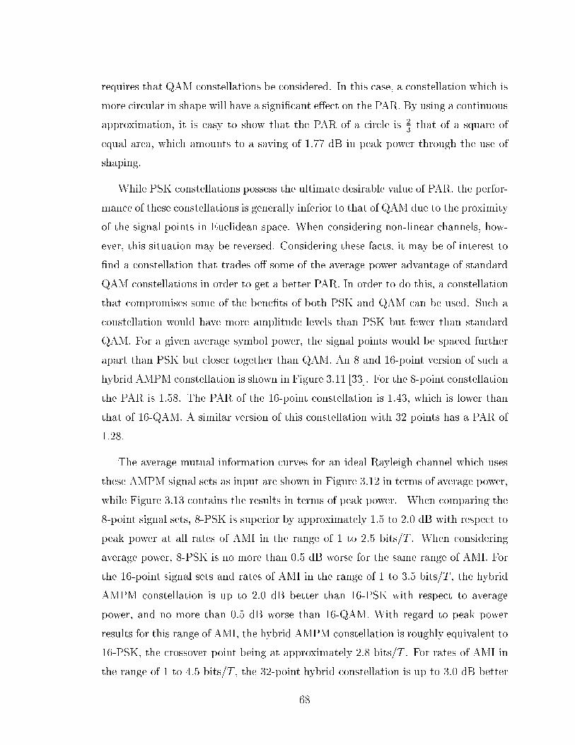
requires that QAM constellations be considered. In this case, a constellation which is
more circular in shape will have a signi�cant e�ect on the PAR. By using a continuous
approximation, it is easy to show that the PAR of a circle is 23that of a square of
equal area, which amounts to a saving of 1.77 dB in peak power through the use of
shaping.
While PSK constellations possess the ultimate desirable value of PAR, the perfor-
mance of these constellations is generally inferior to that of QAM due to the proximity
of the signal points in Euclidean space. When considering non-linear channels, how-
ever, this situation may be reversed. Considering these facts, it may be of interest to
�nd a constellation that trades o� some of the average power advantage of standard
QAM constellations in order to get a better PAR. In order to do this, a constellation
that compromises some of the bene�ts of both PSK and QAM can be used. Such a
constellation would have more amplitude levels than PSK but fewer than standard
QAM. For a given average symbol power, the signal points would be spaced further
apart than PSK but closer together than QAM. An 8 and 16-point version of such a
hybrid AMPM constellation is shown in Figure 3.11 [33]. For the 8-point constellation
the PAR is 1.58. The PAR of the 16-point constellation is 1.43, which is lower than
that of 16-QAM. A similar version of this constellation with 32 points has a PAR of
1.28.
The average mutual information curves for an ideal Rayleigh channel which uses
these AMPM signal sets as input are shown in Figure 3.12 in terms of average power,
while Figure 3.13 contains the results in terms of peak power. When comparing the
8-point signal sets, 8-PSK is superior by approximately 1.5 to 2.0 dB with respect to
peak power at all rates of AMI in the range of 1 to 2.5 bits/T . When considering
average power, 8-PSK is no more than 0.5 dB worse for the same range of AMI. For
the 16-point signal sets and rates of AMI in the range of 1 to 3.5 bits/T , the hybrid
AMPM constellation is up to 2.0 dB better than 16-PSK with respect to average
power, and no more than 0.5 dB worse than 16-QAM. With regard to peak power
results for this range of AMI, the hybrid AMPM constellation is roughly equivalent to
16-PSK, the crossover point being at approximately 2.8 bits/T . For rates of AMI in
the range of 1 to 4.5 bits/T , the 32-point hybrid constellation is up to 3.0 dB better
68
d1
d2
d1
d2
Figure 3.11: Hybrid AMPM Constellations
69

Figure 3.12: AMI of an Ideal Rayleigh Fading Channel in Terms of Average Power:
Hybrid AMPM Constellations
70

Figure 3.13: AMI of an Ideal Rayleigh Fading Channel in Terms of Peak Power:
Hybrid AMPM Constellations
71
than 32-PSK with respect to average symbol energy, and up to 1.9 dB better with
respect to peak power at higher values of AMI. The peak power crossover point with
32-PSK is at approximately 2.5 bits/T . When compared with the 32-CR constellation
for the same rates of AMI, the hybrid constellation is no more than 1.8 dB worse with
respect to average energy, and less than 0.6 dB inferior with respect to peak power.
The peak power crossover point with 32-CR is at about 2.9 bits/T , where the hybrid
constellation is up to 1 dB better at low values of AMI. Considering these results, the
hybrid AMPM signal sets are an attractive alternative to the standard constellations
for use over fading channels. By adjusting the number of amplitude levels and the
spacing between them, these constellations can be tailored to provide the desired level
of performance.
3.4.2 Channel Capacity with a Peak Power Constraint
The problem of determining the absolute limit on the rate of communication over an
ideal fading channel with a peak power constraint is diÆcult to solve. In order to
calculate the capacity, one may try to use the average mutual information expression
given in equation (3.25). Since H(N) does not depend on the probability distribution
of the input, it is only necessary to choose p(x) to maximize H(Y j�) subject to a
peak power constraint. Unfortunately, this does not work out as nice mathematically
as in the case of when an average power constraint is imposed. An alternate approach
is to calculate upper and lower bounds on the channel capacity. In order to do this,
results which were stated in [1] are utilized.
The average power of a random variable X is de�ned to be EX = E fjXj2g.Shannon de�nes the entropy power PX of a random variable X to be the power of
a Gaussian random variable with entropy H(X). If X actually happens to be a
Gaussian random variable, then EX = PX . Using the fact that H(X) = ln�ePXwhen X is Gaussian, the entropy power of X can be expressed in the form
PX =1
�eH(X)�1: (3.42)
For a �xed value of average power, a Gaussian distributed random variable maximizes
entropy. So in general for any random variable X, EX � PX , where equality holds
72

only if X is Gaussian. The results required in order to calculate bounds on channel
capacity are stated here.
Theorem 3.3 Let Z and N be two independent random variables with average power
EZ and EN , respectively. Assume that at least one of the variables has a zero mean.
If Y = Z + N , then the entropy power of the variable Y can be bounded from above
by
PY � EZ + EN (3.43)
where equality holds only if Z and N are both Gaussian. This inequality will be
referred to as the entropy power bound.
Proof: Since Z and N are independent, the variance of Y will equal the sum of the
variances of Z and N . Therefore, EY � EZ + EN where equality holds when either
Z or N have a zero mean. Since the entropy power PY is less than or equal to the
average power EY , equation (3.43) follows. Also, PY = EY when Y is Gaussian,
which means that Z and N must also be Gaussian for equality in (3.43) to hold. 2
Theorem 3.4 Let Z and N be two independent random variables with entropy power
PZ and PN , respectively. If Y = Z + N , then the entropy power of the variable Y
can be bounded from below by
PY � PZ + PN (3.44)
where equality holds only if Z and N are both Gaussian. This inequality will be
referred to as the entropy power inequality.
Proof: The proof of this theorem is quite involved. Shannon used variational methods
in [1] to show that for given values of PZ and PN , the entropy power has a stationary
point when Z and N are both Gaussian. Shannon's approach, however, did not
account for the possibility that other distributions might yield an equal or lower
value of PY . The �rst rigorous proof of this theorem is credited to Stam [52], and an
improved version is due to Blachman [53]. 2
Over a fading channel, the received symbol Y is the sum of two independent
random variables, the �rst being the product �X of the fading process and channel
symbol, and the second being the noise process N . Suppose for the moment that the
73
value of the fading variable is �xed at � = �. Since � is assumed to be known at the
receiver, the entropy power of Y conditioned on � can be expressed as
PY j� =1
�eH(Y j�=�)�1: (3.45)
From equation (3.43), this entropy power can be bounded by PY j� � EZj�+EN where
the random variable Z is equal to the product �X. The equality in this expression is
met for a �xed value of � when Y is Gaussian with variance 12(EZj� + EN). This is
possible only when, for a �xed value of �, both Z and N are Gaussian with variances
of 12EZj� and 1
2EN , respectively. Using this inequality, the entropy can be bounded
from above by
H(Y j� = �) � lnh�e(EZj� + EN)
i: (3.46)
Using the fact that I(X;Y j� = �) = H(Y j� = �) � H(N) and H(N) = ln�eEN ,
the average mutual information is bounded from above by
I(X;Y j� = �) � ln
1 +
EZj�EN
!: (3.47)
Given a peak power constraint on the input, the upper bound on AMI can be ex-
pressed as
I(X;Y j� = �) � ln
1 +
PZj�EN
!(3.48)
where PZj� is the peak power of Z for a �xed value of �. This inequality is obtained
from the fact that average power is always less than or equal to peak power, and from
the monotonicity of the logarithm. By setting PZj� = j�j2Ps, where Ps is the peakpower of the channel input x, and representing the average noise power by EN = N0,
the upper bound to capacity is obtained by averaging equation (3.48) over the pdf
p(�). The resulting upper bound on channel capacity with a peak power constraint
is
CU = Ep(�)
�log2
�1 + j�j2 Ps
N0
��bits=T: (3.49)
This expression is very similar to that for the channel capacity given an average power
constraint. If the peak power of the input is �xed at Ps, then the average power will
be less than or equal to Ps, and the capacity will be less than that obtained with a
Gaussian input that has a variance of 12Ps. Using the results in Appendix B.1, the
74

upper bound on capacity for an ideal Rayleigh channel with a peak power constraint
is
CU = � (log2 e) exp
0@" �Ps
N0
#�11AEi0@�
"�PsN0
#�11A bits=T: (3.50)
A lower bound on channel capacity may be obtained through use of the entropy
power inequality PY j� � PZj� + PN . By substituting in the appropriate expressions
for entropy power, the inequality becomes
1
�eH(Y j�=�)�1 � 1
�eH(Zj�=�)�1 +
1
�eH(N)�1: (3.51)
This inequality can be rearranged into the form
H(Y j� = �) � ln�eH(Zj�=�) + eH(N)
�: (3.52)
In order to get a tight bound, it is desirable to choose the input distribution so that
H(Zj� = �) is maximized. Given a peak power constraint of jXj2 � Ps, the entropy
H(Zj� = �) is maximized by choosing the input to be uniformly distributed on a
circle of radiuspPs. This is accomplished by setting p(zj�) = 1
�j�j2Ps for jzj � j�jpPs,which results in the entropy H(Zj� = �) = ln�j�j2Ps. By substituting this into
equation (3.52) along with the entropy expression for the noise variable N , the lower
bound on the entropy of Y conditioned on a �xed value of � becomes
H(Y j� = �) � ln��j�j2Ps + �eEN
�: (3.53)
Using this result, the lower bound on average mutual information for a �xed value of
� is
I(X;Y j� = �) � ln�1 + j�j2 Ps
eEN
�: (3.54)
By averaging this inequality over the fading variable and converting the logarithm to
base 2, the resulting lower bound takes on the form
CL = Ep(�)
�log2
�1 + j�j2 Ps
eN0
��bits=T: (3.55)
By making use of the results in Appendix B.1, the lower bound on capacity for an
ideal Rayleigh channel with a constraint on peak power is determined to be
CL = � (log2 e) exp
0@" �Ps
eN0
#�11AEi0@�
"�PseN0
#�11A bits=T: (3.56)
75

The upper and lower bounds obtained here for the ideal Rayleigh fading channel
are plotted in Figure 3.14. The capacity of an ideal Rayleigh fading channel subject to
a peak input power constraint is located somewhere in between these two curves. For
large values of SNR, the power gap between the two bounds is a factor of e, which is
equivalent to approximately 4.34 dB. In terms of achievable data rate, this discrepancy
is no more than 1.44 bits/T . If one could obtain an average mutual information curve
for a speci�c input distribution, then the resulting AMI curve could be used to replace
the lower bound obtained here and reduce the gap between the limits on capacity.
3.5 Channels with Space Diversity
Diversity combining is often used in mobile communication systems in order to reduce
the possibility of outage or loss of channel. This is usually accomplished by means of
space diversity, where L antennae are used to receive a given transmitted signal. If
one of the antennae should experience a deep fade in signal level, then the likelihood
that all of them are also experiencing a deep fade at the same time will diminish as
L increases. The focus of this section is the e�ect of space diversity on the capacity
and average mutual information of a multipath fading channel.
It is assumed that when a symbol x is transmitted, the L symbols yk = �kx + nk
for k = 1; : : : ; L are received over parallel channels. Since these parallel channels are
considered to be ideal, it is also assumed that the receiver has knowledge of the fading
variables �k for k = 1; : : : ; L. In the case of maximal-ratio combining, estimates of
the fading variables are actually used in calculating the weighting coeÆcients. Given
knowledge of the additional received symbols over other antennae, the entropy of the
random variable X should decrease, resulting in a proportional increase in average
mutual information. The form of the average mutual information that is of interest
here is
I(X;YLj�L) = E
(log
p(x; y1; : : : ; yLj�1; : : : ; �L)p(x)p(y1; : : : ; yLj�1; : : : ; �L)
)(3.57)
where YL is used to denote the set of random variables (Y1; : : : ; YL) representing
the received symbols, �L denotes the set of random fading variables (�1; : : : ;�L),
and expectation is taken over the joint pdf p(x; y1; : : : ; yL; �1; : : : ; �L). A collection of
76

Figure 3.14: Bounds on the Capacity of an Ideal Rayleigh Fading Channel with a
Peak Power Constraint
77
symbols such as YL = (Y1; : : : ; YL) will be viewed here either as an ordered L-tuple of
symbols or as a 1� L matrix. This is often done in linear algebra, and the intended
interpretation will be de�ned by the context in which the symbol is used. The average
mutual information can also be expressed as the di�erence of entropies
I(X;YLj�L) = H(YLj�L)�H(YLjX;�L): (3.58)
By factoring the conditional pdf speci�ed in equation (3.4) into product form and
using properties of the logarithm, a joint entropy can be expressed as a sum. Doing
so for the entropies in equation (3.58) results in the expression
I(X;YLj�L) =LXk=1
H(YkjYk�1;�k)�LXk=1
H(YkjYk�1; X;�k) (3.59)
which can also be written as
I(X;YLj�L) =LXk=1
I(Yk;XjYk�1;�k): (3.60)
In these expressions, Yk represents the subset of k symbols (Y1; : : : ; Yk), and �k
represents the subset of k fading variables (�1; : : : ;�k). Finally, equation (3.60) can
be written in the form
I(X;YLj�L) = I(Y1;Xj�1) +LXk=2
I(Yk;XjYk�1;�k): (3.61)
Since average mutual information is always greater than or equal to zero, and the
AMI due to a single diversity channel is given by the term I(Y1;Xj�1), the in-
crease in average mutual information due to diversity is given by the expressionPLk=2 I(X;YkjYk�1; �k).
In order to compare the results for di�erent levels of diversity, it is necessary to
de�ne an average received signal-to-noise ratio. This is de�ned here as the sum of the
average SNR observed on each antenna. For the kth antenna, the average received
signal power is de�ned to be �Esk = Efj�kj2jXj2g, or equivalently �Esk = 2�2�kEs. The
average received noise power is assumed to be the same for all antennae, since any
di�erence can always be absorbed into the fading variable �k. For additive white
Gaussian noise, the received noise power is simply N0 = 2�2N . By taking the ratio
of these two power terms, the average SNR for the kth antenna is determined to be
78
�EskN0
=�2�k
Es
�2N
. In order to compare the fading levels experienced by each antenna, it
is assumed that �2�k = ak�2� for k = 1; : : : ; L. Using this assumption, the average
received SNR is expressed as
�EsN0
=LXk=1
ak�2�Es�2N
: (3.62)
The only case investigated here is for when all ak are equal to 1. If a mobile unit is
constantly in motion, then on average it is reasonable to assume that the channels
associated with the individual antennae are equally good. In this case, the average
received SNR is�EsN0
=L�2�Es�2N
: (3.63)
3.5.1 E�ect of Diversity on Discrete-Input Channels
The e�ect of diversity on the average mutual information of a multipath fading chan-
nel is examined here for the case of when a discrete-valued signal constellation is used
as an input alphabet. The average mutual information can be written as a di�erence
of entropies in the form
I(X;YLj�L) = H(X)�H(XjYL;�L): (3.64)
Suppose the constellation has a uniform a priori distribution over M points. The pmf
which describes this is p(xi) =1M
for i = 1; : : : ;M , and the entropy of the signal set is
H(X) = logM . The conditional entropy H(XjYL;�L) in the expression is obtained
by averaging the logarithm of the conditional pmf p(xijy1; : : : ; yL; �1; : : : ; �L) over
the joint pdf p(xi; y1; : : : ; yL; �1; : : : ; �L). By using Bayes' theorem and the law of
total probability, the conditional pmf of X given Y1; : : : ; YL and �1; : : : ;�L can be
expressed as
p(xijy1; : : : ; yL; �1; : : : ; �L) = p(y1; : : : ; yLjxi; �1; : : : ; �L)p(xi)PMj=1 p(y1; : : : ; yLjxj; �1; : : : ; �L)p(xj)
: (3.65)
After substituting in the pmf for X and factoring the joint density in this expression,
the resulting form of the pmf is
p(xijy1; : : : ; yL; �1; : : : ; �L) =QLk=1 p(ykjyk�1; : : : ; y1; xi; �1; : : : ; �L)PM
j=1
QLl=1 p(yljyl�1; : : : ; y1; xj; �1; : : : ; �L)
: (3.66)
79
If the symbols x and �k are known at the receiver, then the symbol yk = �kx+nk will
not depend on any of the other received symbols or fading variables obtained from
the other antennae. The pmf in equation (3.66) can therefore be simpli�ed to
p(xijy1; : : : ; yL; �1; : : : ; �L) =QLk=1 p(ykjxi; �k)PM
j=1
QLl=1 p(yljxj; �l)
: (3.67)
The constituent pdf's in this expression can be derived from the pdf of the additive
white Gaussian noise as was done in equation (3.20), and take the form
p(ykjxi; �k) = 1
2��2Nexp
�jyk � �kxij2
2�2N
!: (3.68)
By substituting these pdf's into equation (3.67) and simplifying, the resulting prob-
ability mass function is
p(xijy1; : : : ; yL; �1; : : : ; �L) =exp
��1
2
�PLk=1
jyk��kxij2�2N
��PMj=1 exp
��1
2
�PLl=1
jyl��lxj j2�2N
�� : (3.69)
The conditional entropy of X given YL and �L is then determined to be
H(XjYL;�L) =1
M
MXi=1
E
8<:log
24 MXj=1
exp
�
LXk=1
jyk � �kxjj2 � jyk � �kxij22�2N
!359=;(3.70)
where expectation is taken over the joint pdf p(y1; : : : ; yL; �1; : : : ; �Ljxi). Since the
received symbol on each antenna is yk = �kx+nk for k = 1; : : : ; L, by substituting this
into equation (3.70), averaging can be performed over the distribution of the noise
variables Nk rather than the conditional distribution of the Yk given knowledge of X
and the �k. By using this fact, the resulting form of the average mutual information
in bits/T is
I(X;YLj�L) = log2M� 1
M
MXi=1
E
8<:log2
24 MXj=1
exp
�
LXk=1
j�k(xi � xj) + nkj2 � jnkj22�2N
!359=;
(3.71)
where expectation is taken over p(n1) : : : p(nL)p(�1; : : : ; �L).
In order to ascertain the e�ects of space diversity on the AMI of channels with
discrete-valued input, the expression in equation (3.71) was evaluated by computer
simulation for the case of an ideal Rayleigh fading channel. The input alphabets
80

Diversity=2 Diversity=3
8-PSK 16-QAM 8-PSK 16-QAM
3.5 - 2.5 dB - 0.8 dB
3 - 1.6 dB - 0.5 dB
AMI 2.5 2.2 dB 1.2 dB 0.6 dB 0.3 dB
(Bits/T ) 2 1.4 dB 0.9 dB 0.4 dB 0.3 dB
1.5 0.9 dB 0.7 dB 0.3 dB 0.3 dB
1 0.6 dB 0.6 dB 0.2 dB 0.1 dB
Table 3.7: Average Power Gain Due to Increase in Space Diversity of Rayleigh Fading
Channel
considered were 8-PSK and 16-QAM constellations. To ensure that the average SNR
is equal for all antennae and that the fading has a unity gain, it is assumed that all the
noise variables Nk have variance �2N and that the variances �2�k of the fading variables
�k all have a value of 12L. By ensuring that E fjXj2g = 1, the SNR is completely
speci�ed by the value of �2N .
The �rst case considered is that of uncorrelated fading between individual anten-
nae. Figure 3.15 shows the AMI curves for when 8-PSK is used over an ideal Rayleigh
channel with a space diversity of 1, 2, and 3. Figure 3.16 shows the curves for the
case of when a 16-QAM constellation is used. The average power gains due to an
increase in the level of space diversity are shown in Table 3.7 for various rates of AMI.
These gains counteract a signi�cant portion of the loss due to fading experienced on
single diversity channels. By comparing Table 3.5 with the results in Table 3.7, one
can see that the loss due to fading for 8-PSK at the indicated rates of AMI is in the
range of 1.3 to 3.9 dB for a single diversity channel, from 0.7 to 1.7 dB for a dual
diversity channel, and roughly 0.5 to 1.1 dB for a diversity of three antennae. The
ranges of loss due to fading for 16-QAM are observed by comparing the results in
Table 3.6 with those in Table 3.7, and are determined to be 1.1 to 4.6 dB, 0.5 to 2.1
dB, and 0.4 to 1.3 dB for a diversity of one, two, and three antennae, respectively.
The gains available in going from 2 to 3 antennae are less than those obtained when
increasing from 1 to 2 antennae. For example, at an AMI rate of 2 bits/T with an
81

Figure 3.15: AMI of an Ideal Rayleigh Fading Channel with Space Diversity: 8-PSK
82

Figure 3.16: AMI of an Ideal Rayleigh Fading Channel with Space Diversity: 16-QAM
83
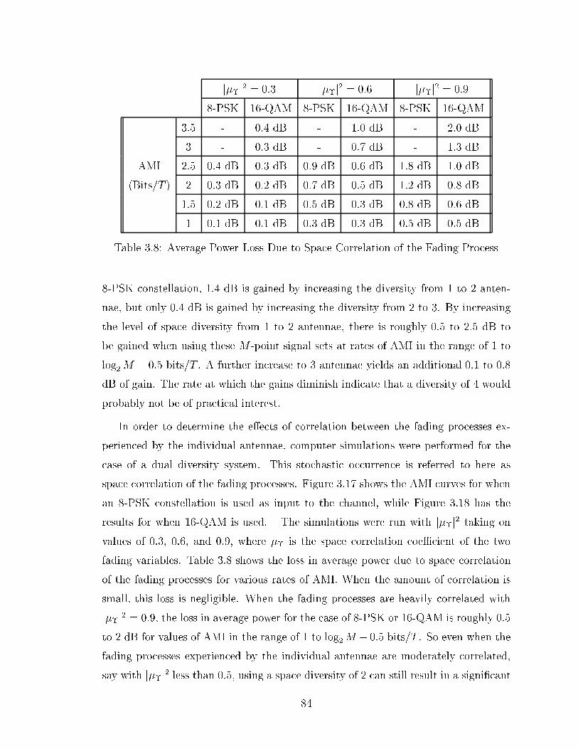
j��j2 = 0:3 j��j2 = 0:6 j��j2 = 0:9
8-PSK 16-QAM 8-PSK 16-QAM 8-PSK 16-QAM
3.5 - 0.4 dB - 1.0 dB - 2.0 dB
3 - 0.3 dB - 0.7 dB - 1.3 dB
AMI 2.5 0.4 dB 0.3 dB 0.9 dB 0.6 dB 1.8 dB 1.0 dB
(Bits/T ) 2 0.3 dB 0.2 dB 0.7 dB 0.5 dB 1.2 dB 0.8 dB
1.5 0.2 dB 0.1 dB 0.5 dB 0.3 dB 0.8 dB 0.6 dB
1 0.1 dB 0.1 dB 0.3 dB 0.3 dB 0.5 dB 0.5 dB
Table 3.8: Average Power Loss Due to Space Correlation of the Fading Process
8-PSK constellation, 1.4 dB is gained by increasing the diversity from 1 to 2 anten-
nae, but only 0.4 dB is gained by increasing the diversity from 2 to 3. By increasing
the level of space diversity from 1 to 2 antennae, there is roughly 0.5 to 2.5 dB to
be gained when using these M -point signal sets at rates of AMI in the range of 1 to
log2M � 0:5 bits/T . A further increase to 3 antennae yields an additional 0.1 to 0.8
dB of gain. The rate at which the gains diminish indicate that a diversity of 4 would
probably not be of practical interest.
In order to determine the e�ects of correlation between the fading processes ex-
perienced by the individual antennae, computer simulations were performed for the
case of a dual diversity system. This stochastic occurrence is referred to here as
space correlation of the fading processes. Figure 3.17 shows the AMI curves for when
an 8-PSK constellation is used as input to the channel, while Figure 3.18 has the
results for when 16-QAM is used. The simulations were run with j��j2 taking on
values of 0.3, 0.6, and 0.9, where �� is the space correlation coeÆcient of the two
fading variables. Table 3.8 shows the loss in average power due to space correlation
of the fading processes for various rates of AMI. When the amount of correlation is
small, this loss is negligible. When the fading processes are heavily correlated with
j��j2 = 0:9, the loss in average power for the case of 8-PSK or 16-QAM is roughly 0.5
to 2 dB for values of AMI in the range of 1 to log2M � 0:5 bits/T . So even when the
fading processes experienced by the individual antennae are moderately correlated,
say with j��j2 less than 0.5, using a space diversity of 2 can still result in a signi�cant
84

Figure 3.17: AMI of an Ideal Rayleigh Fading Channel with Diversity=2 and Space
Correlated Fading: 8-PSK
85

Figure 3.18: AMI of an Ideal Rayleigh Fading Channel with Diversity=2 and Space
Correlated Fading: 16-QAM
86

increase in the average mutual information when discrete-valued signal sets are used
for transmission over an ideal Rayleigh fading channel.
3.5.2 Capacity of Fading Channels with Space Diversity
The e�ect of space diversity is examined here for channels with a continuous-valued
input alphabet. The set of received symbols yL = (y1; : : : ; yL) can be expressed as
a vector equation yL = x�L + nL, where the scalar x is the transmitted symbol,
�L = (�1; : : : ; �L) is a vector of the fading variables associated with each antenna,
and nL = (n1; : : : ; nL) is a vector of the noise variables associated with each antenna.
The average mutual information between the transmitted symbol X and the vector of
received symbols YL, given knowledge of the �L, can be expressed as the di�erence
of entropies
I(X;YLj�L) = H(YLj�L)�H(YLjX;�L): (3.72)
The �rst term considered in this expression is the conditional entropy H(YLjX;�L).
If the variables X and �L are known, then the joint entropy of YL conditioned on
these variables is the same as the joint entropy of the vector of noise variables NL.
The general form of a L-dimensional complex-valued Gaussian density, which is used
here to describe the additive noise vector, is
p(nL) =1
(2�)L detBNexp
��1
2n�LB
�1N nTL
�(3.73)
where BN is a L � L covariance matrix with entries (BN)ij = 12EfNiN
�j g. Since
the noise variables are assumed to be independent, BN is a diagonal matrix with
the non-zero entries being equal to (BN )ii = �2N . By computing the value of the
entropy H(NL) = �Ep(nL)flog p(nL)g, the entropy of YL conditioned on X and �L
is determined to be
H(YLjX;�L) = logh(2�e)L detBN
i: (3.74)
As in the case of a single random variable, given a constraint on the second order
moments of a set of L complex-valued random variables, the entropy is maximized
by a L-dimensional complex-valued Gaussian distribution. In order to calculate the
value of the entropy H(YLj�L), it is �rst necessary to determine the pdf p(yLj�L).
87
This is accomplished by starting with the pdf of the additive noise vector given in
equation (3.73). Since yk = �kx + nk for k = 1; : : : ; L, the conditional pdf of Y L
given knowledge of �L and X is
p(yLj�L; x) = 1
(2�)L detBNexp
��1
2(yL � x�L)
�B�1N (yL � x�L)
T�
(3.75)
which is obtained from p(nL) by performing a vector translation. For the moment, it
is assumed that the input alphabet has a Gaussian distribution. The desired pdf can
then be obtained by evaluating the integral
p(yLj�L) =ZSXp(yLj�L; x)p(x)dx: (3.76)
By substituting in the expressions for the required probability densities, this integral
can be written explicitly as
p(yLj�L) = AZSX
exp
�1
2
"1
�2X+ ��LB
�1N �
TL
#jxj2
!exp
�<nxy�LB
�1N �
TL
o�dx
(3.77)
where A = 1(2�)L+1�2
XdetBN
exp��1
2y�LB
�1N yTL
�. Transforming the variable x into polar
coordinates, where � = jxj and � = arg x, equation (3.77) can be expressed in the
form
p(yLj�L) = AZ 1
0� exp
�1
2
"1
�2X+ ��LB
�1N �
TL
#�2!
(3.78)
�Z 2�
0exp
��<
ny�LB
�1N �
TL
ocos � � �=
ny�LB
�1N �
TL
osin �
�d�d�
where <f�g and =f�g denote the real and imaginary parts of the enclosed complex-
valued expression, respectively. By making use of relation 3.937 2. taken from [54],
the integral with respect to � can easily be solved as
Z 2�
0exp
��<
ny�LB
�1N �
TL
ocos � � �=
ny�LB
�1N �
TL
osin �
�d� = 2�I0
����y�LB�1N �
TL
��� �� :(3.79)
By changing the variable � topu in equation (3.78), and using the result in equation
(3.79), the pdf can be expressed in the form
p(yLj�L) = �AZ 1
0exp
�1
2
"1
�2X+ �
�LB
�1N �
TL
#u
!I0����y�LB�1
N �TL
���pu� du: (3.80)
88

By viewing this integral as the Laplace transform of I0����y�LB�1
N �TL
���pu�, it is evalu-ated to be [55, p. 197 (14)]
p(yLj�L) = 2��2XA1 + �2X�
�LB
�1N �
TL
exp
0B@ �2X
���y�LB�1N �
TL
���22�1 + �2X �
�LB
�1N �
TL
�1CA : (3.81)
By substituting in the value of A and simplifying, the desired pdf is determined to
be
p(yLj�L) = 1
(2�)L detBY j�exp
��1
2y�LB
�1Y j�y
TL
�(3.82)
which is a Gaussian distribution. The covariance matrix BY j� consists of the entries
(BY j�)ij = �i��j�
2X for i 6= j, and (BY j�)ii = j�ij2�2X +�2N along the diagonal. The de-
terminant of this matrix is detBY j� = (1+�2X ��LB
�1N �
TL ) detBN . Since the resulting
distribution is Gaussian, the entropy of Y L conditioned on �L can be immediately
written as
H(YLj�L) = Ep(�L)
nlog
h(2�e)L detBN
�1 + �2X�
�LB
�1N �
TL
�io: (3.83)
By substituting the entropies obtained into equation (3.72), the average mutual in-
formation is determined to be
I(X;YLj�L) = Ep(�L)
nlog
�1 + �2X�
�LB
�1N �
TL
�o: (3.84)
Recalling the results for the single diversity channel, the pdf p(ykj�k) will be Gaussianonly if p(x) is. If this is not the case, then the marginal densities p(ykj�k) as well asthe joint density will not be Gaussian. Since this is the distribution that maximizes
H(YLj�L) subject to a constraint on the second order moments, capacity is achieved
for an ideal fading channel with space diversity by a Gaussian distributed input.
Thus, equation (3.84) speci�es the capacity of the channel. Assuming that the average
received SNR is the same for each antenna, the capacity can be written in bits/T as
C = Ep(�L)
(log2
1 +
�2X�2N
LXk=1
j�kj2!)
: (3.85)
Averaging over p(�L) in this capacity expression can be explicitly evaluated for the
case of Rayleigh fading. Since the fading variables in this expression occur separately
as terms in a summation, a new random amplitude fading variable R can be de�ned
89

where R2 =PLk=1 j�kj2. The capacity can then be expressed as an average over the
pdf of R, as given by the equation
C = Ep(r)
(log2
1 + r2
�2X�2N
!): (3.86)
This expression is the same as that derived for the case of a single antenna. Since
the �k are independent Gaussian variables with zero mean, the pdf of the variable R
is a central chi distribution with 2L degrees of freedom. By constraining the second
moment of the variable so that E fR2g = 1, this pdf can be written in the form
p(r) =2LLr2L�1
�(L)exp
��Lr2
�for r � 0 (3.87)
which is the same as the Nakagami pdf in equation (2.23) with m = L and = 1.
Therefore, an ideal Rayleigh fading channel with space diversity is equivalent to an
ideal Nakagami fading channel. Using the results of Appendix B.2, equation (3.86)
is evaluated to be
C = (log2 e)(�L)L�(L)
"�EsN0
#�L d
ds
!L�1 �es
sEi(�s)
�bits=T (3.88)
where s = L�
�EsN0
��1. For a dual diversity channel, the closed form expression for
capacity is
C = (log2 e)
241 +
0@2
"�EsN0
#�1� 1
1A exp
0@2
"�EsN0
#�11AEi0@�2
"�EsN0
#�11A35 bits=T:
(3.89)
For a diversity of three antennae, the capacity is expressed in the form
C = �1
2(log2 e)
hs� 3 + (s2 � 2s+ 2) exp (s)Ei (�s)
ibits=T (3.90)
where the parameter s is equal to 3�
�EsN0
��1. Finally, for the case L = 4, the channel
capacity is determined to be
C =1
6(log2 e)
hs2 � 4s+ 11 +
�s3 � 3s2 + 6s� 6
�exp (s)Ei (�s)
ibits=T (3.91)
where s = 4�
�EsN0
��1.
These results are plotted in Figure 3.19 along with the capacity for the AWGN
channel. Also included is the capacity of the Rayleigh channel with no space diversity.
90

Figure 3.19: Capacity of an Ideal Rayleigh Fading Channel with Space Diversity
91

By using the results presented in Appendix C, the asymptotic power loss due to
amplitude fading compared to the AWGN channel is determined to be Le� (L), and
the gain achieved through the use of space diversity is eCE�Le� (L). A dual diversity
system results in a 1.33 dB asymptotic gain, and is no more than 1.17 dB from the
AWGN channel results. For a system which uses three antennae, the asymptotic
diversity gain is 1.74 dB, and the channel capacity is 0.76 dB from the AWGN results.
For the case of four antennae, the asymptotic diversity gain is 1.94 dB, and the
distance from the AWGN channel capacity is 0.56 dB. As L ! 1, the e�ect of
amplitude fading diminishes to the point where capacity is the same as that of an
AWGN channel.
The expression for channel capacity given by equation (3.85) was also evaluated
by means of computer simulation for the case of a dual diversity channel with space
correlated fading. The results obtained for di�erent levels of correlation are shown in
Figure 3.20. These results once again indicate that even when the fading processes
experienced by the individual antennae are moderately correlated, the resulting loss
is small. When the space correlation coeÆcient is set so that j��j2 = 0:3, the loss
compared to the uncorrelated case is 0.2 dB. For a value of j��j2 = 0:6 the loss is
approximately 0.6 dB, and when j��j2 = 0:9 the loss is roughly 1.0 dB.
A result was presented in [34] which was intended to represent the capacity of
an ideal Rayleigh fading channel with space diversity. Although the end results are
similar to those derived here, the formulation of the problem was di�erent. The ex-
pression used for capacity was that of a AWGN channel. The SNR was modelled
as being a random variable based on maximal ratio combining, with statistics de-
termined by the level of diversity. The pdf describing the SNR was a chi-squared
distribution essentially equivalent to the pdf shown in equation (3.87). Although no
explicit expression for the channel capacity was given, the necessary averaging was
performed through computer simulation, and the curves presented were equivalent to
those derived here.
Examination of the results shown in this section indicate that a signi�cant gain in
capacity is obtained by using a dual diversity system. From a practical standpoint,
however, it is not likely that the small additional potential gains associated with
92

Figure 3.20: Capacity of Dual Diversity Rayleigh Channel with Space Correlated
Fading
93

higher levels of diversity would warrant the increase in complexity and cost. The
actual number of antennae used in any system will likely be governed by the desired
outage probability.
3.6 Potential Coding Gain for Fading Channels
Up to this point, the limits on reliable communication have been determined for
a number of ideal fading channel models. In this section, these limits are used to
determine the magnitude of the coding gain that can be expected over a fading
channel. The expression for the capacity of an ideal fading channel is
C = Ep(�)nlog2
�1 + j�j2SNR
�obits=T: (3.92)
At high values of SNR, the channel coding theorem states that an arbitrarily small
probability of error can be realized as long as the data rate Rc in bits/T satis�es the
relation
Rc < Ep(�)nlog2
�j�j2SNR
�o: (3.93)
Since a rate ofRc bits/T requires a constellation of size 2Rc, a signal-to-noise ratio nor-
malized with respect to the constellation size can be de�ned as SNRnorm = 2�RcSNR.
By using this de�nition, equation (3.93) can be rearranged into the form
SNRnorm > 2�Ep(�)flog2(j�j2)g: (3.94)
This result indicates that an arbitrarily small probability of error can be attained as
long as the normalized SNR is greater than the asymptotic fading loss of the channel.
Since the fading process is assumed to have a unity gain, for the ideal Rayleigh channel
this means that SNRnorm > eCE , which is equivalent to 2.51 dB.
This capacity bound can be compared to the symbol error probability of uncoded
QAM in order to determine the potential coding gain available. The probability of
symbol error is closely estimated by the expression
Pr(e) = 1� 2p1 + � �1
�1� 2
�arctan
�q1 + � �1
��(3.95)
where � = 32SNRnorm. This expression is derived in Appendix D.1 and is actually
an upper bound, but becomes more accurate as the size of the signal set grows.
94
The symbol error probability for uncoded QAM is compared to the capacity bound
in Figure 3.21. Due to the almost inverse linear nature of this error probability, the
distance with respect to SNR between the error probability curve and channel capacity
increases dramatically as Pr(e) gets smaller. The ultimate shape gain for the AWGN
channel is approximately 1.53 dB, and is obtained by using a Gaussian distributed
input rather than a square constellation of equal average energy. Since the average
received symbol energy is Efj�Xj2g = 2�2�Es, amplitude fading has no e�ect on
shape gain, so it is the same for a fading channel as it is for the AWGN channel. If the
1.53 dB of shape gain is subtracted from the di�erence between the channel capacity
and the error probability curve for QAM, the remainder represents the potential
coding gain over uncoded QAM. At a symbol error rate of 10�3, the potential coding
gain is about 23.3 dB. For small values of Pr(e) this increases dramatically; roughly
10 dB for every decrease in error probability by a power of 10. At a symbol error
rate of 10�6 the potential gain is approximately 53.3 dB, and increases to 73.3 dB for
Pr(e) = 10�8.
The potential coding gain for fading channels is extremely large compared to the
AWGN channel. In general, much of this gain is realized by known bandwidth eÆcient
coding techniques, but the performance of these known codes is still signi�cantly far
from capacity. It may be of interest to see where the best known codes stand against
capacity results. Since most research has focussed on achieving spectral eÆciencies
of 2 bits/T using an 8-PSK constellation, these results are examined here. The AMI
curve for 8-PSK in Rayleigh fading indicates that 2 bits/T can be achieved with an
arbitrarily small probability of error for an average bit SNR greater than 5.4 dB.
The bit SNR is 3 dB less than the symbol SNR for a rate of 2 bits/symbol. This
bound on AMI is compared to the bit error performance of a number of coding
schemes in Figure 3.22. The schemes considered are Ungerboeck's 8-state 8-PSK
trellis code [6], Zehavi's suboptimal 8-state 8-PSK code [21], and Lin's multi-level
block coded scheme [22]. Also included is the bit error probability of uncoded QPSK
modulation with Gray coding. In Appendix D.2 this is shown to be given by the
95
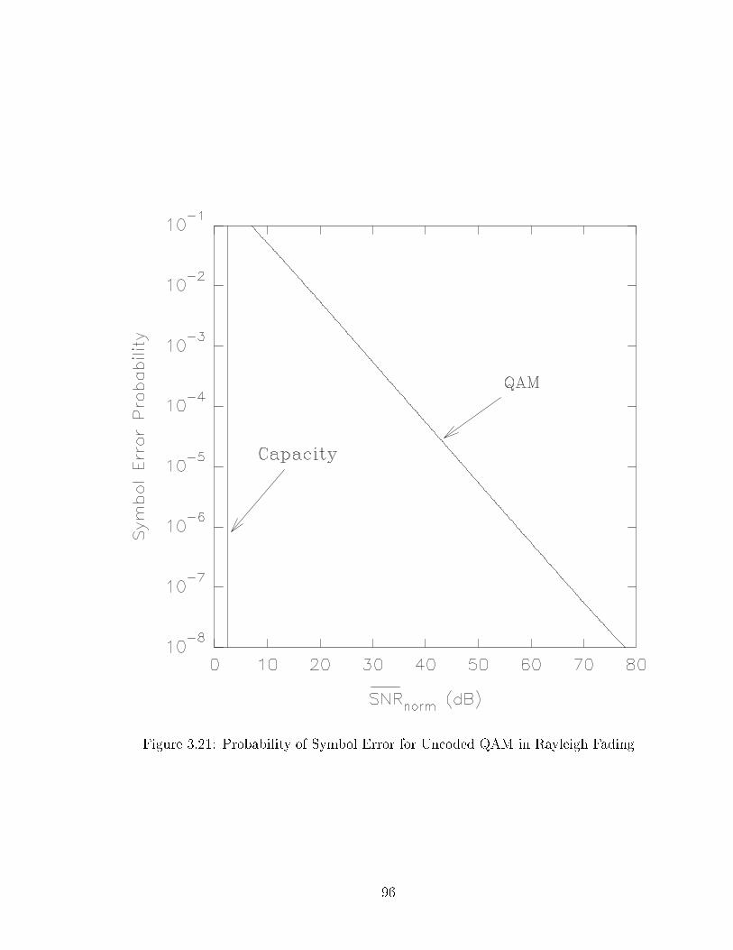
Figure 3.21: Probability of Symbol Error for Uncoded QAM in Rayleigh Fading
96

Figure 3.22: Bit Error Probability in Rayleigh Fading for Various Coded Modulation
Schemes with Rate 2 bits/T
97

expression
Pb =1
2
26641� 1r
1 +h�EbN0
i�13775 (3.96)
where�EbN0
is the average SNR per bit. At a bit error rate of 10�6, the distance
between the AMI curve for 8-PSK and the bit error curve corresponding to QPSK is
roughly 48.6 dB. Ungerboeck's code reduces this distance to 18.5 dB. Zehavi's code
is approximately 11.4 dB away from capacity at this error rate, and Lin's code is
approximately 6.6 dB away. Even the best known result leaves 6.6 dB of potential
gain, which is signi�cant. In general, there is much more to be gained at higher
spectral eÆciencies when larger signal constellations are considered.
Figure 3.23 contains the bit error probability curves for the recently published
turbo codes designed for use in Rayleigh fading [23]. The curve labelled TC1 is for
the code which transmits 2 bits/T using a 16-QAM constellation. The corresponding
capacity curve for 16-QAM at this rate is labelled C1. For a bit error probability
of 10�5, the turbo code is 4.4 dB from capacity. The bit error curve labelled TC2
is for the turbo code which transmits 3 bits/T using a 16-QAM constellation. The
corresponding capacity curve for this rate using 16-QAM is labelled C2. This code
attains a bit error probability of 10�5 at a SNR which is 5.1 dB from capacity. The
�nal error curve labelled TC3 is for the code which transmits 4 bits/T using 64-QAM.
The corresponding capacity curve for a rate of 4 bits/T using 64-QAM is labelled C3.
For a bit error rate of 10�5, this code is also 5.1 dB from capacity. These are the best
known coding results to date.
98

Figure 3.23: Bit Error Probability in Rayleigh Fading for Turbo Codes
99

Chapter 4
E�ects of Non-Ideal Channel State
Information
Having determined the achievable rates of data transmission over ideal fading chan-
nels, the next logical step is to consider practical limitations to this idealization and
the resulting consequence to reliable communication. In the previous chapter, a fad-
ing channel was de�ned to be ideal if it satis�ed four conditions. In this chapter it
is assumed that the fading channel model still satis�es all of these conditions except
for the postulate concerning channel state information. This means that the value
of the fading variable � is no longer assumed to be available at the receiver. This
assumption of non-ideal channel state information (CSI) re ects the reality of hav-
ing to estimate information about the fading process using some practical scheme
at the receiver. Rather than determining the fading variable � exactly, an estimate
is obtained. The requirement of a channel state estimate is demonstrated through
calculation of average mutual information for discrete-valued constellations, as well
as an upper bound on this quantity for continuous-valued input alphabets. These
numbers turn out to be quite small when no information is available about the fading
process and most of the received energy is due to scattered signal components. The
�rst instance of non-ideal CSI investigated is for the case of perfect phase information
with no amplitude information. This model is based upon the assumption of perfect
coherent detection with no attempt made to determine the fading level. The AMI for
standard constellations is obtained and compared to the ideal channel results in order
to determine the amount of loss which results when the fading amplitude is ignored.
100

Bounds on average mutual information are also calculated for the phase information
case when a continuous-valued input is used. In order to investigate the e�ects of
practical channel estimation schemes, the true value of � and the channel estimate
are modelled as jointly Gaussian random variables. The variance of the estimate, as
well as the correlation coeÆcient between the true and estimated values, are depen-
dent upon the particular method used. The schemes considered here are the use of a
pilot tone, di�erentially coherent detection, and the use of a pilot symbol. The loss
incurred due to the limitations of these estimation techniques is ascertained through
calculation of AMI for channels using standard constellations.
4.1 Requirement of Channel State Estimation
In this section, the need for channel state estimation is exhibited through calculation
of information theoretic quantities. It has been demonstrated that reduced knowledge
of the fading variable � results in a performance loss of certain types of coded and
uncoded modulation [16]. It is conceivable, however, that a scheme may exist which
achieves reliable communication at an arbitrary rate when no CSI is used in detection.
4.1.1 Channels with Discrete-Valued Input and No CSI
Consider the AMI when a discrete-valued constellation is used as input to a fading
channel, and where the value of the fading variable � is unknown at the receiver.
The AMI between the input X and the output Y can be expressed as a di�erence
of entropies by the equation I(X;Y ) = H(X) � H(XjY ), where H(X) = logM for
an equiprobable input distribution. In order to determine the entropy H(XjY ), thepmf p(xijy) is required. This probability mass function can be obtained by starting
with the pdf of the fading variable �. A Rayleigh fading channel is considered �rst,
which means that � will be a zero mean complex-valued Gaussian random variable
with pdf
p(�) =1
2��2�exp
� j�j
2
2�2�
!: (4.1)
101

If a new variable Z is de�ned as being equal to the product �X, then the pdf of Z
given knowledge of the value of X can be determined from equation (4.1) to be
p(zjxi) = 1
2�jxij2�2�exp
� jzj22jxij2�2�
!: (4.2)
This is obtained by scaling the random variable � by the complex number xi. Since
the channel output can be written as the sum y = z + n, the pdf of the variable Y
given knowledge of X and N is
p(yjxi; n) = 1
2�jxij2�2�exp
� jy � nj22jxij2�2�
!(4.3)
which is obtained from equation (4.2) by performing a translation on the variable z.
The complex-valued noise variable N is described by a zero mean Gaussian distri-
bution with variance �2N . As was shown in the previous chapter, evaluation of the
integralRSNp(yjxi; n)p(n)dn is simply a convolution of the two density functions. In
this case, application of equation (3.31) results in the conditional pdf
p(yjxi) = 1
2�(�2�jxij2 + �2N)exp
� jyj22(�2�jxij2 + �2N )
!: (4.4)
Using Bayes' theorem in conjunction with the law of total probability, and the as-
sumption that p(xi) =1M
for i = 1; : : : ;M , one may write the desired pmf in the
form
p(xijy) = p(yjxi)PMj=1 p(yjxj)
: (4.5)
The entropy H(XjY ) = �Ep(xi;y) flog p(xijy)g can then be determined from the ex-
pression
H(XjY ) = Ep(xi;y)
(log
"PMj=1 p(yjxj)p(yjxi)
#): (4.6)
By substituting the pdf given by (4.4) into equation (4.6) and simplifying, this be-
comes
H(XjY ) = (4.7)
1M
PMi=1
RSYp(yjxi) log
�PMj=1
�2�jxij2+�2N�2�jxjj2+�2N
exp�� jyj2�2�(jxij2�jxj j2)
2(�2�jxij2+�2N )(�2�jxj j2+�2N )
��dy:
Averaging over p(yjxi) in this expression can be replaced by expectation taken over
p(�)p(n). This is accomplished by setting y = �xi+n in equation (4.7), which results
102

in the conditional entropy being expressed as
H(XjY ) = 1
M
MXi=1
E
8<:log
24 MXj=1
�2�jxij2 + �2N�2�jxjj2 + �2N
exp
� j�xi + nj2�2�(jxij2 � jxjj2)2(�2�jxij2 + �2N)(�
2�jxjj2 + �2N)
!359=; :
(4.8)
The form of this entropy expression lends insight into the general magnitude of
the achievable rates of AMI for Rayleigh fading channels with discrete-valued input
and no information about the fading variable. For the ideal fading channel, this
entropy is a function of the Euclidean distances between signal points. With no CSI
available at the receiver, the entropy depends upon the di�erence of the magnitudes of
the various symbols. For constant envelope modulation, such as in the case of PSK,
the symbol magnitudes are all equal. In this case the equivocation of the channel
is H(XjY ) = logM , which is the same as the entropy H(X) of the input, and the
resulting AMI of the channel is I(X;Y ) = 0. Therefore, observation of the channel
output without any CSI does not reduce the average uncertainty of which PSK symbol
is transmitted, and on average, no information is transmitted over the channel.
The AMI was also determined through computer simulation for the case of when
certain multi-level constellations are used as input to the channel. Even at an average
received SNR of 40 dB, the AMI achievable using 16-QAM is approximately 0.29
bits/T , while a rate of 0.32 bits/T is attained by using a 32-CR constellation.
Examination of equation (4.8) reveals that the use of multi-level signal sets cannot
improve the AMI to a very large degree. For a �xed value of X = xi, consider the
term log2
�PMj=1 exp
�� j�(xi�xj)+nj2�jnj2
2�2N
��, which comes from the expression given in
equation (3.22) for the equivocation of an ideal fading channel. For large values of
SNR, all the exponential terms tend to zero except for the one in which xj = xi,
which has a value of 1. Therefore, the logarithm approaches a value of zero, which in
turn causes the equivocation of the channel to vanish. The corresponding expression
for a channel with no CSI is log2
�PMj=1
�2�jxij2+�2N�2�jxj j2+�2N
exp�� j�xi+nj2�2N (jxij2�jxj j2)
2(�2�jxij2+�2N )(�2�jxj j2+�2N )
��. In
this case, not only the term in which xj = xi will yield a value of 1, but so will any
other term involving a signal point with the same magnitude as xi. For those signal
points which have a di�erent magnitude than that of xi, the resulting term in the
summation over j will approach a value of approximately jxij2jxj j2 exp
�1� jxij2
jxj j2�for large
values of SNR. Subject to an average power constraint of the form 1M
PMi=1 jxij2 = 1,
103

one can see that the equivocation of a Rayleigh fading channel with no CSI cannot
be made arbitrarily small. As the size of the constellation is made larger, the signal
points become increasingly crowded together. This causes larger numbers of channel
symbols to have relatively equivalent magnitudes.
Due to the low potential data rates for a Rayleigh channel with no CSI, it is of
interest to determine similar results for the case of when a LOS component exists
in the received signal. If the pdf shown in equation (4.1) is given a non-zero mean
m�, then by following the same procedure shown for the Rayleigh case, the AMI of
a Rician channel expressed in units of bits/T is determined to be
I(X;Y ) = log2M� (4.9)
1M
PMi=1E
�log
�PMj=1
�2�jxij2+�2N�2�jxj j2+�2N
exp��1
2
�j�xi�m�xj+nj2�2�jxjj2+�2N
� j(��m�)xi+nj2�2�jxij2+�2N
����:
For a non-zero mean m�, there is a dependence upon the weighted distance between
discrete channel symbols. As the Rician channel parameter R spans the range from
0 to1, the AMI curves span the range delimited by the Rayleigh and AWGN results.
The expression for AMI in equation (4.9) was evaluated by computer simulation
for di�erent values of R. The resulting AMI curves for when an 8-PSK signal set is
used as input to the channel are shown in Figure 4.1. Similar results for 16-QAM are
shown in Figure 4.2. In order to interpret these results, one may view the receiver as
using the LOS component of the signal for synchronization, but completely ignoring
the e�ect of the scattered multipath components. When R = 5 dB, up to 1.9 bits/T
can be transmitted using an 8-PSK constellation, while a maximum rate of 2.4 bits/T
occurs for the case of 16-QAM. A Rician channel parameter of R = 10 dB allows
maximum rates of 2.7 bits/T and 3.4 bits/T to be attained using 8-PSK and 16-QAM
signal sets, respectively.
4.1.2 Channel with Continuous-Valued Input and No CSI
An upper bound on average mutual information may also be calculated in order to
determine the achievable rate of communication without CSI. An upper bound to the
AMI I(X;Y ) = H(Y )�H(Y jX) is determined here for a Rayleigh fading channel with
a continuous-valued input. The �rst step in accomplishing this is to bound the term
104
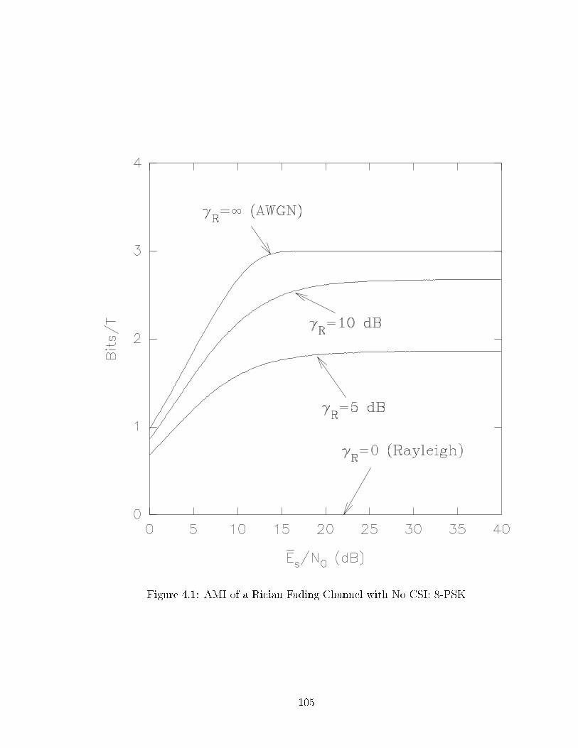
Figure 4.1: AMI of a Rician Fading Channel with No CSI: 8-PSK
105

Figure 4.2: AMI of a Rician Fading Channel with No CSI: 16-QAM
106

H(Y ) from above. The entropy power bound was presented in the previous chapter,
and stated that the entropy power of a sum of two independent random variables is
less than or equal to the sum of the average power of the individual variables. Since
the channel output symbol can be expressed as Y = Z +N , where EfjZj2g = 2�2�Es
and EfjN j2g = 2�2N , the entropy power bound can be used here to write
PY =1
�eH(Y )�1 � 2�2�Es + 2�2N : (4.10)
This expression can also be stated in the form
H(Y ) � lnh2�e
��2�Es + �2N
�i: (4.11)
In order for the equality in (4.11) to hold, there must exist a random variable X
with pdf p(x) and second moment 12Es such that the product Z = �X is a Gaussian
variable. The existence of such a distribution for X has not been determined here.
In order to determine an upper bound on �H(Y jX), or equivalently a lower bound
to H(Y jX), the entropy power inequality will be invoked. For a conditional entropy
it is obvious that
H(Y jX) � Ep(x)nlnheH(ZjX=x) + eH(N)
io: (4.12)
This is true because the entropy power inequality can be applied when X is �xed,
and the averaging necessary to obtain H(Y jX) does not a�ect the inequality. In [53],
a relation referred to as \the log cosh inequality" can be used to further show that
H(Y jX) � Ep(x)nlnheH(ZjX=x) + eH(N)
io� ln
heH(ZjX) + eH(N)
i: (4.13)
As stated previously, the entropy of the additive Gaussian noise is H(N) = ln 2�e�2N .
By examining the pdf given by equation (4.2), one can see that p(zjx) is Gaussian,so the conditional entropy of Z given knowledge of X can be written as
H(ZjX) = Ep(x)nln�2�e�2�jxj2
�o= ln
�2�e�2�
�+ Ep(x)
nln jxj2
o: (4.14)
Since the natural logarithm is a concave function, one can apply Jensen's inequal-
ity [49, p. 25] to obtain the relation
Ep(x)nln jxj2
o� ln
hEp(x)
njxj2
oi(4.15)
107

where equality holds only when jxj2 is constant for all values of x. This inequality
can also be expressed in the form
Ep(x)nln jxj2
o= lnEs ��J (4.16)
where �J is a non-negative constant which is independent of the energy in the signal.
To show that this is true, one need only scale the variable x used in equation (4.15).
The scale factor then manifests itself as an identical additive constant on both sides
of the inequality. By subtracting this additive term from both sides, one obtains
the original inequality. Substituting the relation given by (4.16) into equation (4.14)
results in the entropy expression
H(ZjX) = ln�2�e1��J�2�Es
�: (4.17)
The lower bound on the conditional entropy of Y given knowledge of X is obtained
by substituting the required entropies into (4.13). This results in the relation
H(Y jX) � lnh2�e
�e��J�2�Es + �2N
�i: (4.18)
By substituting the bounds shown in (4.11) and (4.18) into the di�erence of entropies
expression, the resulting upper bound on AMI is determined to be
IU = log2
24 1 +
�EsN0
1 + exp (��J)�EsN0
35 bits=T (4.19)
where�EsN0
=�2�Es�2N
. For large values of SNR, IU � �J log2 e. Therefore, no matter how
much energy is used, the capacity cannot exceed a certain constant value.
Unfortunately, the entropy power relations result in very weak bounds for certain
distributions. Therefore, the expression in (4.19) cannot be used to obtain a good
bound on capacity. It is possible, however, to calculate the value of �J for certain
speci�c distributions which result in a small limiting value of AMI. When p(x) is
Gaussian, the number �J is equal to Euler's constant, which results in the AMI
being bounded to less than 0.83 bits/T . When X has a uniform distribution over a
circle centered at the origin, this constant equals �J = 1 � ln 2, which bounds the
AMI to less than 0.44 bits/T .
108

If the Gaussian fading variable is assumed to have a non-zero mean m�, and the
upper bound in equation (4.19) is rederived, then this bound as applied to the Rician
fading channel takes the form
IU = log2
24 1 +
�EsN0
1 + exp(��J )1+ R
�EsN0
35 bits=T: (4.20)
This upper limit on AMI is plotted in Figure 4.3 for various values of the Rician
channel parameter R. The value of �J used is that derived for a Gaussian distributed
input. As R !1, this bound becomes increasingly precise. For large values of SNR,
this bound will be approximately IU � (log2 e)�J + log2(1 + R). When a Gaussian
distributed input is used, the AMI is less than 2.9 bits/T for R = 5 dB and less than
4.3 bits/T for R = 10 dB.
As an illustration of how the bound in equation (4.19) can be made arbitrarily
poor, consider the following case [56]. De�ne the random variable � to equal jXj2. Thediscrepancy in Jensen's inequality can be represented in this case by the expression
�J = lnhEp(�) f�g
i� Ep(�) fln �g : (4.21)
Now if � has a lognormal distribution described by the pdf
p(�) =1q
2��2��exp
�(ln � �m�)
2
2�2�
!for � > 0 (4.22)
then Ep(�) f�g = exp�m� +
�2�2
�and Ep(�) fln �g = m�. In this case, the expression
in (4.21) evaluates to �J =�2�2, which can be made arbitrarily large by choosing �2� to
be arbitrarily large. Any power constraint can be applied independently by choosing
an appropriate value for m�. For example, to set E f�g = 1, choose m� = ��2�2.
Thus, even though this result indicates that capacity is limited to being less than
some constant value, the bound is extremely weak in some cases.
4.2 Channels with Phase-Only Information
The results of the previous section show that for a Rayleigh fading channel with no
CSI available at the receiver, most of the information in the signal amplitude and
109

Figure 4.3: Upper Bounds on the AMI of a Rician Fading Channel with No CSI:
Gaussian Distributed Input
110

all the information in the phase is lost. In this section it is assumed that the phase
of the fading process is known at the receiver, but that the amplitude is not. This
model will be referred to as a channel with phase-only information or a phase-only
channel. A somewhat practical realization of this model would be a coherent receiver
that can track the variations of the phase of the fading process. Since no e�ort is
made to determine the fading amplitude, the implementation of such a receiver would
be less complex, and this would likely result in the system being less expensive. The
phase-only information assumption was referred to as a channel with no CSI in the
work of Simon and Divsalar [16]. Information theoretic bounds on communication
rate are determined �rst for channels using discrete-valued input, then for channels
with continuous-valued input.
4.2.1 Phase-Only Channels with Discrete-Valued Input
The AMI of a fading channel with discrete-valued input and phase-only information is
determined here by evaluating the familiar di�erence of entropies expression, which in
this case is written I(X;Y j�) = H(X)�H(XjY;�). As usual, an equiprobable input
distribution is assumed over a M -point constellation, which results in the entropy of
the channel input beingH(X) = logM . In order to determine the entropyH(XjY;�),an expression for the pmf p(xijy; �) must be found. This probability mass function is
obtained here by �rst �nding the pdf p(yjxi; �), then applying Bayes' theorem. The
pdf of the additive noise variable N will be used here as a point of departure in the
derivation of p(yjxi; �). Starting with the probability density function
p(n) =1
2��2Nexp
� jnj
2
2�2N
!(4.23)
and setting y = �xi + n, the conditional pdf of Y given knowledge of � and X can
be determined by performing a translation on n. The resulting pdf is
p(yjxi; �) = 1
2��2Nexp
�jy � �xij2
2�2N
!: (4.24)
Knowledge of the fading variable � means knowledge of both the magnitude variable
R and the phase variable �. By setting � = rej� in equation (4.24), the pdf can be
111

assumed to be conditioned on both R and �, which results in the density function
being expressed as
p(yjxi; r; �) = 1
2��2Nexp
�jy � rej�xij2
2�2N
!: (4.25)
This can also be written in the form
p(yjxi; r; �) = 1
2��2Nexp
� jyj
2
2�2N
!exp
�jxij
2
2�2Nr2!exp
0@<
nye�j�x�i
o�2N
r
1A : (4.26)
The motivation for writing the pdf in this fashion is the desire for evaluating the
integral p(yjxi; �) =Rp(yjxi; r; �)p(r)dr, which eliminates the dependence on the
fading amplitude. Under the assumption of Rayleigh fading, the statistics of the
amplitude R are described by the pdf
p(r) =r
�2�exp
� r2
2�2�
!for r � 0: (4.27)
The desired probability density function can be placed in the form
p(yjxi; �) = (4.28)
12��2
��2N
exp�� jyj2
2�2N
� R10 r exp
���jxij22�2
N
+ 12�2
�
�r2�exp
�<fye�j�x�ig
�2N
r�dr:
In order to simplify notation in the evaluation of the integral in this expression,
the following substitutions are made. Let the �rst variable be �i =�2�jxij2+�2N
2�2��2N
and
de�ne the second variable to be �i =jyj2+jxij2�jy�ej�xij2
2�2N
. The subscripts on �i and �i
are used to indicate the dependence of these parameters upon a particular channel
symbol xi. Ignoring this dependence for the moment, the integral in equation (4.28)
can be expressed as Z 1
0r exp
���r2 + �r
�dr: (4.29)
By completing the square and factoring, this integral becomes
exp
�2
4�
! Z 1
0r exp
0@��
r � �
2�
!21A dr: (4.30)
Making the substitution t = r � �2�
breaks this into the sum
exp
�2
4�
!Z 1
� �2�
t exp���t2
�dt+
�
2�exp
�2
4�
!Z 1
� �2�
exp���t2
�dt: (4.31)
112

The �rst integral in this expression is evaluated to equal 12�, while the second can
be placed in a more familiar form. By letting s =p2�t, the second integral in this
expression can be written
�p2�
(2�)3=2
Z 1
� �p2�
1p2�
exp
�s
2
2
!ds: (4.32)
This integral represents the area under a Gaussian pdf with zero mean and unit
variance taken over the interval�� �p
2�;1
�. This fact allows the expression in (4.32)
to be written in the form
�p2�
(2�)3=2
"1
2+Z �p
2�
0
1p2�
exp
�s
2
2
!ds
#: (4.33)
Making the �nal substitution of variables u = sp2results in
�
2
r�
�exp
�2
4�
!"1 +
Z �
2p�
0
2p�exp
��u2
�du
#: (4.34)
The remaining integral is erf�
�2p�
�, where erf(�) is the well-known error function.
Referring back to the integral in equation(4.28), it is evaluated to be
1
2�
"1 +
�
2
r�
�exp
�2
4�
!"1 + erf
�
2p�
!##: (4.35)
Therefore, the conditional pdf of Y given knowledge of X and � is
p(yjxi; �) = 1
2�(�2�jxij2 + �2N )exp
� jyj
2
2�2N
!"1 +
�i2
s�
�iexp
�2i4�i
!"1 + erf
�i
2p�i
!##:
(4.36)
Using this density function along with Bayes' theorem and the law of total probability,
one may obtain the pmf p(xijy; �) = p(yjxi;�)PM
j=1p(yjxj ;�)
. This can then be used to evaluate
the conditional entropy
H(XjY;�) = (4.37)
1M
PMi=1
RRp(yjxi; �)p(�)log
2664PM
j=1
(�2�jxij2+�2N )
�1+
�j2
q��j
exp
��2j
4�j
�h1+erf
��j
2p�j
�i�
(�2�jxj j2+�2N )
�1+
�i2
p��i
exp
��2i
4�i
�h1+erf
��i
2p�i
�i�3775d�dy:
By making the substitution y = rej�xi+n in this expression, averaging over the joint
density p(yjxi; �)p(�) can be replaced by expectation taken over the joint pdf p(�)p(n)
113

Number of Signal Points
4 8 16 32
4.5 - - - 0.0 dB
4 - - - 0.1 dB
3.5 - - 0.1 dB 0.1 dB
AMI 3 - - 0.1 dB 0.2 dB
(Bits/T ) 2.5 - 0.3 dB 0.2 dB 0.2 dB
2 - 0.3 dB 0.3 dB 0.3 dB
1.5 0.5 dB 0.5 dB 0.4 dB 0.4 dB
1 0.7 dB 0.6 dB 0.6 dB 0.6 dB
Table 4.1: Loss of SNR Due to Phase-Only Information: PSK Constellations
of the fading variable and the additive noise variable. The AMI for a discrete-valued
input channel with phase-only information can then be expressed in units of bits/T
as
I(X;Y j�) = log2M� (4.38)
1M
PMi=1Ep(�)p(n)
8>><>>:log2
2664PM
j=1
(�2�jxij2+�2N )
�1+
�j2
q��j
exp
��2j
4�j
�h1+erf
��j
2p�j
�i�
(�2�jxj j2+�2N )
�1+
�i2
p��i
exp
��2i
4�i
�h1+erf
��i
2p�i
�i�37759>>=>>;
where averaging over p(�)p(n) can be easily accomplished by computer simulation.
Since �4�
gets very large for small values of SNR, the term exp��2j4�2j
� �2i4�2i
�should be
factored out in equation (4.38) in order to prevent numerical over ow during computer
simulation.
The expression for AMI in equation (4.38) was evaluated for three types of sig-
nal constellation. The results for PSK constellations are shown in Figure 4.4. The
curves for the case of phase-only information appear to be identical to those for the
ideal channel. Table 4.1 contains the loss in average SNR for various rates of AMI.
In general, the loss for PSK constellations is roughly 0.6 dB at a rate of 1 bit/T
and decreases for higher rates of AMI. At small values of SNR, the unknown fading
amplitude acts in conjunction with the additive noise to degrade performance. This
causes the AMI to be slightly lower than that achieved over the ideal channel, but
114

Figure 4.4: AMI of a Phase-Only Rayleigh Fading Channel: PSK Constellations
115

Number of Signal Points
16 32 64
5.5 - - 13.6 dB
5 - - 9.0 dB
4.5 - 7.2 dB 6.7 dB
4 - 5.1 dB 5.2 dB
AMI 3.5 5.7 dB 3.9 dB 3.9 dB
(Bits/T ) 3 3.1 dB 2.9 dB 3.0 dB
2.5 2.0 dB 2.0 dB 2.2 dB
2 1.5 dB 1.4 dB 1.6 dB
1.5 1.0 dB 1.0 dB 1.1 dB
1 0.8 dB 0.8 dB 0.9 dB
Table 4.2: Loss of SNR Due to Phase-Only Information: QAM Constellations
this e�ect vanishes with increasing SNR.
The standard QAM constellations are the second category of signal set considered.
The AMI curves are shown in Figure 4.5 for various sizes of signal constellation. In
this case there is a dramatic di�erence compared to the ideal fading channel. The
loss in SNR due to lack of knowledge of the fading amplitude is stated in Table 4.2
for various rates of AMI. In general, the loss at 1 bit/T is approximately 1 dB and
increases for higher rates of AMI. The losses at a rate of log2M � 1 bits/T for a
M -point constellation are 5.7 dB, 5.1 dB, and 9.0 dB for M equal to 16, 32, and 64,
respectively. Another noticeable e�ect is that the AMI curves tend to a maximum
value which is less than log2M . This maximum value is in fact approximately equal
to the entropy of the phase of the discrete-valued constellation. For the 16-QAM
signal set, there are 12 di�erent phase values, 8 of which occur with a probability of
0.0625 and 4 of which occur with a probability of 0.125. The entropy of the phase is
easily calculated to be 3.5 bits/T . This can be compared to the AMI of the channel
for a SNR of 40 dB, which equals 3.73 bits/T . Similarly, the entropy of the phase of
the 32-CR and 64-QAM signal sets is 4.75 bits/T and 5.5 bits/T , respectively. The
respective values of AMI for these constellations at a SNR of 40 dB is 4.84 bits/T and
116

Figure 4.5: AMI of a Phase-Only Rayleigh Fading Channel: QAM Constellations
117

Number of Signal Points
8 16 32
4.5 - - 3.2 dB
4 - - 2.8 dB
3.5 - 2.4 dB 2.3 dB
AMI 3 - 2.1 dB 1.7 dB
(Bits/T ) 2.5 1.6 dB 1.7 dB 1.2 dB
2 1.4 dB 1.3 dB 0.8 dB
1.5 1.1 dB 0.9 dB 0.7 dB
1 0.9 dB 0.8 dB 0.67 dB
Table 4.3: Loss of SNR Due to Phase-Only Information: Hybrid AMPM Constella-
tions
5.57 bits/T for 32-CR and 64-QAM. Using these constellations to transmit log2M
bits/T over a channel with phase-only information should result in a noticeable error
oor in performance.
Due to the large losses incurred for high values of AMI when using QAM constel-
lations, it is of interest to determine the achievable rates when the hybrid AMPM
signal sets introduced in section 3.4.1 are used as input to the channel. The AMI
curves for channels using these constellations are shown in Figure 4.6. The loss in
SNR for various �xed values of AMI are shown in Table 4.3. For the 8-point constel-
lations, when the losses due to lack of knowledge of the fading variable are considered,
8-PSK is superior by roughly 0.2 to 0.8 dB for values of AMI in the range of 1 to
2.5 bits/T . The 16-point constellations are more or less equivalent. For rates of AMI
in the range of 1 to 3.5 bits/T , 16-PSK is no more than 0.4 dB better. For the case
of 32 signal points, the two types of constellation are essentially indistinguishable for
rates of AMI in the range of 1 to 4.5 bits/T , with the PSK constellation being no
more than 0.1 dB better.
In practice, it is unlikely that the phase of a 32-PSK constellation could be tracked
e�ectively by a coherent receiver. So for any practical system which attempts to track
the phase but ignores the amplitude of the fading process, the spectral eÆciency will
118

Figure 4.6: AMI of a Phase-Only Rayleigh Fading Channel: Hybrid AMPM Constel-
lations
119

likely be limited to less than 4 bps/Hz. To surpass this rate, it appears that an e�ort
must be made to determine the amplitude of the fading process as well as the phase.
4.2.2 Phase-Only Channels with Continuous-Valued Input
The focus now turns to phase-only information channels with a continuous-valued
input. Since channel capacity is not easily calculated, an upper bound on AMI will
be used instead. By writing the average mutual information of the channel in the
form I(X;Y j�) = H(Y j�) �H(Y jX;�), an upper bound is obtained by separately
bounding each of the entropies in this expression then adding the results. When the
channel output symbol is expressed as the sum y = rej�x + n, the entropy power
bound can be used to limit the entropy power of Y to being less than the sum of
the average power of each term. Notice that EfjRej�Xj2g = 2�2�Es regardless of the
value of �. Using this along with EfjN j2g = 2�2N , which is the average power of the
additive noise, the entropy power bound may be written as
H(Y j�) � lnh2�e
��2�Es + �2N
�i: (4.39)
To obtain a lower bound on H(Y jX;�), the entropy power inequality will be usedin the form
H(Y jX;�) � lnheH(ZjX;�) + eH(N)
i: (4.40)
Since H(N) is known to be ln 2�e�2N , only H(ZjX;�) needs to be determined, where
the variable Z is de�ned to be equal to the product �X. In order to calculate this
entropy, the following result will be used. If � is a complex-valued random variable
and X = x is a constant, then the entropy power of the product �X is [49, p. 233]
H(�X) = H(�) + log jxj2: (4.41)
This is easily proven by examining the expression for entropy and using a change of
variables. With knowledge of this result one can write H(ZjX;�) = H(�XjX;�),and this yields the form
H(ZjX;�) = H(�j�) + Ep(x)nlog jxj2
o: (4.42)
120

If X happens to be a random variable, then equation (4.41) is also averaged over p(x),
which yields the result in equation (4.42). By using Jensen's inequality as was done
in the previous section, one can make the substitution Ep(x) flog jxj2g = log e��JEs,
where �J is the magnitude of the discrepancy in the inequality. Since the fading
variable is � = Rej�, then if the phase � is known at the receiver, all of the uncertainty
is in the fading amplitude R. Therefore, the substitution H(�j�) = H(R) can be
made, where the entropy H(R) is that of a Rayleigh variable. Using the fundamental
de�nition of entropy, one can substitute in the pdf p(r) and calculate
H(R) = 1 + ln��p2+CE
2(4.43)
where CE is Euler's constant. An adjustment to this entropy must be made before
substituting it back into equation (4.42). As was stated earlier, the entropy of a
continuous-valued random variable is dependent upon the coordinate system used.
The expression in equation (4.42) is taken with respect to a Cartesian coordinate
system, whereas the entropy in (4.43) is evaluated in a polar coordinate system. By
using the de�nition of entropy and performing a change of variables, the entropyH(R)can be stated in rectangular coordinates by subtracting the term Ep(r;�)
nlogJ
�polrect
�ofrom the result in (4.43). In this expression, J
�polrect
�represents the Jacobian of the
transformation. In particular J�polrect
�= 1
rand Ep(r;�)
nlog 1
r
o= ln 1p
2��+ CE
2. So in
rectangular coordinates, the entropy of the fading amplitude R is H(�j�) = ln e�2�.
Referring back to equation (4.42), the entropy may be written
H(ZjX;�) = ln e1��J�2�Es: (4.44)
The lower bound on the entropy H(Y jX;�) can be determined from equation (4.40)
to be
H(Y jX;�) � ln
"2�e
e��J
2��2�Es + �2N
!#: (4.45)
Using this result, the upper bound on average mutual information can be written in
bits/T as
I(X;Y j�) � IU = log2
24 1 +
�EsN0
1 + exp(��J)2�
�EsN0
35 (4.46)
where�EsN0
=�2�Es�2N
.
121

This upper bound on AMI is plotted in Figure 4.7 for the case of a Gaussian
distributed input. Also shown is the capacity curve for the ideal Rayleigh fading
channel. The AMI for this continuous-valued input asymptotically approaches a
maximum value which is less than that achieved by some discrete-valued input chan-
nels. This result seems surprising at �rst, since for most practical channel models a
continuous-valued input can be used to attain higher values of AMI. However, upon
further examination of the situation, this result makes perfect sense. Consider the
upper bound in (4.46) as the signal-to-noise ratio gets large. This is estimated to be
log2 2�+�J log2 e. The second term of this sum was obtained for the case of no CSI,
and is an upper bound on the AMI when only the signal amplitude is considered. The
�rst term is the entropy of a uniformly distributed phase variable, and is therefore an
upper bound on the AMI transmitted through the phase of the signal. For the case
of a M -PSK constellation, by choosing M large enough and by using a suÆciently
high SNR, the equivocation of the channel can be made very small, which results in
the AMI approaching a value of log2M . For a continuous-valued phase distribution,
a maximum entropy of log2 2� bits/T is achieved by a uniform distribution. If the
equivocation of the channel is made very small, the maximum AMI in the phase can
be no greater than log2 2� bits/T .
4.3 Realistic Channel Estimation Methods
The remainder of this chapter will deal with fading channels in which the CSI is
provided at the receiver by some practical channel estimation method. The statistics
of the channel estimate are speci�ed by a model which was used in [35] for the purpose
of analyzing the performance of TCM. It is assumed that the fading variable � is a
complex-valued Gaussian random variable. Since the focus will be on a Rayleigh
fading channel, the pdf of � will be the same as that stated in equation (4.1). Let
~� be an estimate of � determined by some realistic channel estimation scheme. The
general form of the channel estimate for the methods considered here can be written
as ~� = ��� + n, where � is a complex-valued scale factor, n is additive noise, and ��
is the value taken on by the fading process at a time duration � prior to when ~� is
122

Figure 4.7: Bounds on AMI for a Phase-Only Rayleigh Channel with Continuous-
Valued Input
123

determined. As usual, the noise is assumed to be Gaussian with a zero mean. Due to
this form, it is reasonable to assume that ~� is also Gaussian with the same zero mean
value as �. If a LOS component exists in the signal, then ~� will have a non-zero
mean that is scaled by �. Based on these assumptions, the channel estimate ~� will
be assumed to be described by the pdf
p(~�) =1
2��2~�exp
�j
~�j22�2~�
!: (4.47)
It is also assumed that � and ~� are jointly Gaussian random variables. The joint pdf
describing this is
p(�; ~�) =1
(2�)2(1� j�j2)�2��2~�exp
� 1
2(1� j�j2)
" j�j2�2�
� 2<f���~��g���~�
+j~�j2�2~�
#!:
(4.48)
The parameter � is the correlation coeÆcient between � and ~�, and is de�ned as
� =C�~�
�2��2~�
, where C�~� = 12En�~��
o. If the value of the random variable ~� is known,
then the conditional pdf of � given ~� = ~� is
p(�j~�) = 1
2�(1� j�j2)�2�exp
0@� j� � ���~�
�~�j2
2(1� j�j2)�2�
1A (4.49)
which is obtained by dividing the joint pdf given in equation (4.48) by the pdf in
equation (4.47). This density function can be used to determine the pdf p(yjx; ~�),which in turn is used to calculate the AMI of the channel. If a new random variable
Z is de�ned to equal the product �X, then given knowledge of X and ~�, the pdf of
Z is
p(zjx; ~�) = 1
2�(1� j�j2)jxj2�2�exp
0@� jz � ���~�x
�~�j2
2(1� j�j2)jxj2�2�
1A (4.50)
which is obtained by scaling the variable �. Since the channel output symbol is
y = z + n, then also given knowledge of the value of N , the pdf of Y is
p(yjx; ~�; n) = 1
2�(1� j�j2)jxj2�2�exp
0@� jy �
���~�x�~�
� nj22(1� j�j2)jxj2�2�
1A : (4.51)
Evaluation of the integralRSNp(yjx; ~�; n)p(n)dn is once again a convolution between
two complex-valued Gaussian pdf's. When this is evaluated, the resulting pdf is
p(yjx; ~�) = 1
2�[(1� j�j2)jxj2�2� + �2N ]exp
0@� jy � ���~�x
�~�j2
2[(1� j�j2)jxj2�2� + �2N ]
1A : (4.52)
124

This probability density function can be used in the calculation of AMI for a chan-
nel with discrete-valued input. Assuming that the distribution of the input alpha-
bet is uniform with p(xi) = 1M
for i = 1; : : : ;M , then the entropy of the input
is simply H(X) = logM . The entropy of the input given knowledge of the out-
put and channel state estimate is H(XjY; ~�) = �E flog p(xijy; ~�)g, where the pmf
p(xijy; ~�) =PMj=1
p(yjxj ;~�)p(yjxi;~�) is obtained from p(yjxi; ~�) through application of Bayes'
theorem and the law of total probability. Substituting equation (4.52) into this en-
tropy expression results in
H(XjY; ~�) = (4.53)
1M
PMi=1
RS~�
RSYp(yjxi; ~�)p(~�) log
"PMj=1
[(1�j�j2)jxij2�2�+�2N ]
[(1�j�j2)jxj j2�2�+�2N ]exp
jy����~�xi
�~�j2
2[(1�j�j2)jxij2�2�+�2N ]
� jy����~�xj�~�
j2
2[(1�j�j2)jxj j2�2�+�2N ]
1A35 dyd~�:
By making the substitution y = �xi + n in equation (4.53), the integration can be
replaced by expectation taken over p(�; ~�)p(n), and can be accomplished by means
of computer simulation. By substituting the required entropies into the di�erence
equation I(X;Y j~�) = H(X)�H(XjY; ~�), the AMI of the channel can be written in
units of bits/T as
I(X;Y j~�) = log2M� (4.54)
1M
PMi=1E
(log2
"PMj=1
[(1�j�j2)jxij2�2�+�2N ]
[(1�j�j2)jxj j2�2�+�2N ]exp
j�xi+n����~�xi
�~�j2
2[(1�j�j2)jxij2�2�+�2N ]
� j�xi+n����~�xj�~�
j2
2[(1�j�j2)jxj j2�2�+�2N ]
1A359=; :
This is the general form of the AMI of a channel with CSI provided by a practical
channel estimation method. When considering a particular type of channel estimation
scheme, slight modi�cations to equation (4.54) may be required. Speci�c channel state
estimation techniques are considered next, where expressions are determined for the
parameters j�j2 and �2~�, as well as the required modi�cations to equation (4.54).
125
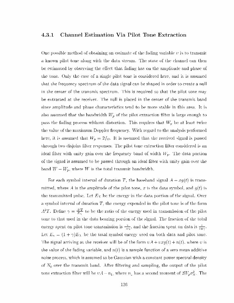
4.3.1 Channel Estimation Via Pilot Tone Extraction
One possible method of obtaining an estimate of the fading variable � is to transmit
a known pilot tone along with the data stream. The state of the channel can then
be estimated by observing the e�ect that fading has on the amplitude and phase of
the tone. Only the case of a single pilot tone is considered here, and it is assumed
that the frequency spectrum of the data signal can be shaped in order to create a null
in the center of the transmit spectrum. This is required so that the pilot tone may
be extracted at the receiver. The null is placed in the center of the transmit band
since amplitude and phase characteristics tend to be more stable in this area. It is
also assumed that the bandwidth Wp of the pilot extraction �lter is large enough to
pass the fading process without distortion. This requires that Wp be at least twice
the value of the maximum Doppler frequency. With regard to the analysis performed
here, it is assumed that Wp = 2fD. It is assumed that the received signal is passed
through two disjoint �lter responses. The pilot tone extraction �lter considered is an
ideal �lter with unity gain over the frequency band of width Wp. The data portion
of the signal is assumed to be passed through an ideal �lter with unity gain over the
band W �Wp, where W is the total transmit bandwidth.
For each symbol interval of duration T , the baseband signal A + xg(t) is trans-
mitted, where A is the amplitude of the pilot tone, x is the data symbol, and g(t) is
the transmitted pulse. Let EX be the energy in the data portion of the signal. Over
a symbol interval of duration T , the energy expended in the pilot tone is of the form
A2T . De�ne = A2TEX
to be the ratio of the energy used in transmission of the pilot
tone to that used in the data bearing portion of the signal. The fraction of the total
energy spent on pilot tone transmission is 1+
, and the fraction spent on data is 11+
.
Let Es = (1 + )EX be the total symbol energy used on both data and pilot tone.
The signal arriving at the receiver will be of the form �A+ �xg(t) + n(t), where � is
the value of the fading variable, and n(t) is a sample function of a zero mean additive
noise process, which is assumed to be Gaussian with a constant power spectral density
of N0 over the transmit band. After �ltering and sampling, the output of the pilot
tone extraction �lter will be �A+n1, where n1 has a second moment of 2Wp�2N . The
126

correlation coeÆcient � is calculated from the equation
� =En�~��
orE fj�j2gE
nj~�j2
o : (4.55)
Using ~� = �A + n1 as the channel estimate, it is easy to show En�~��
o= 2�2�A,
E fj�j2g = 2�2�, and Enj~�j2
o= 2�2�A
2+2Wp�2N . By substituting these results back
into equation (4.55), the squared norm of the correlation coeÆcient can be written
j�j2 = 1
1 +2Wp�2NA2
: (4.56)
Since A2 = 1+
EsT, equation (4.56) can also be expressed in the form
j�j2 = 1
1 + 1+ WpT
��EsN0
��1 (4.57)
where�EsN0
=�2�Es�2N
.
In order to determine the AMI of the channel, the variance of the estimate is also
required. The value of 12Enj~�j2
ohas already been determined, however, this is not
the same as �2~� as required by equation (4.54). The variances used in determining
AMI are required in units of watts/Hz, whereas the value of Enj~�j2
ois given in watts.
Thus, the quantity Enj~�j2
omust be normalized by the bandwidth of the transmit
spectrum. By observing this fact, the variance �2~� can be obtained by evaluating
�2~� =Enj~�j2
o2W
= �2�A2T +WpT�
2N : (4.58)
Using the relation A2 = 1+
EsT, this variance can also be written as
�2~� =
1 + �2�Es +WpT�
2N (4.59)
which is the form that is used here to evaluate equation (4.54). When determining
the correlation coeÆcient �, normalization of the variables is an unnecessary consid-
eration, since this coeÆcient is immune to scaling.
Before calculating the AMI for a given channel, one more consideration needs to
be addressed. Consider the term �x + n2, which is the received faded data symbol
plus additive noise. The noise term n2 is independent of n1, since the �lters are
127

assumed to be non-overlapping. Due to the fact that part of the whole bandwidth is
required for pilot tone extraction, the variance of the variable n2 is calculated to beW�Wp
W�2N = (1�WpT )�
2N . Therefore, for the case of pilot tone transmission, equation
(4.54) must be modi�ed by replacing �2N with (1�WpT )�2N . The AMI for a channel
with pilot tone estimation can now be calculated by using the parameters determined
here in the equation
I(X;Y j~�) = log2M� (4.60)
1M
PMi=1E
(log2
"PMj=1
[(1�j�j2)jxij2�2�+(1�WpT )�2N ]
[(1�j�j2)jxj j2�2�+(1�WpT )�2N ]exp
j�xi+n����~�xi
�~�j2
2[(1�j�j2)jxij2�2�+(1�WpT )�2N ]
� j�xi+n����~�xj�~�
j2
2[(1�j�j2)jxj j2�2�+(1�WpT )�2N ]
1A359=; :
A normalized fading bandwidth fDT taking on values of 0.01, 0.03, and 0.06 was
considered for the results presented here. Through computer simulation of equation
(4.60), it was shown that for a given fDT , the AMI was relatively insensitive over a
large range of values to variations in the power distribution parameter . In [35], it
was stated that an optimum value of exists for a given fDT when considering error
performance of TCM. It was suggested that setting to 0.1, 0.25, and 0.3 for fDT
taking on respective values of 0.01, 0.03, and 0.06, resulted in optimum performance.
Since the values of suggested are in the range in which the AMI is roughly equal to
the maximum value, they were used for the computer simulations performed in order
to obtain the results presented here.
The AMI curves for the case of 8-PSK are shown in Figure 4.8, while Figure 4.9
contains similar results for a 16-PSK constellation. Simulations were also performed
for 16-QAM and 32-CR constellations, and the results are shown in Figure 4.10 and
Figure 4.11, respectively. The AMI curves seem to exhibit the same behavior for
all constellations considered, and on observation of the results, two relationships are
evident. The �rst is the e�ect of SNR on the channel estimate. This is evident through
the decreasing gap, for increasing values of SNR, between the results for ideal CSI and
those obtained here for pilot tone extraction. As the SNR becomes greater, the CSI
approaches ideal and the AMI approaches a value of log2M . The second e�ect is that
of frequency dispersion, which manifests itself as an increasing discrepancy compared
128
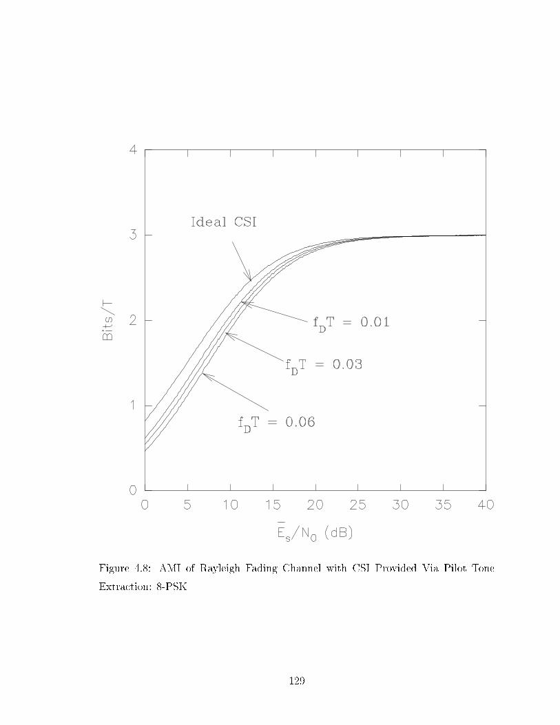
Figure 4.8: AMI of Rayleigh Fading Channel with CSI Provided Via Pilot Tone
Extraction: 8-PSK
129
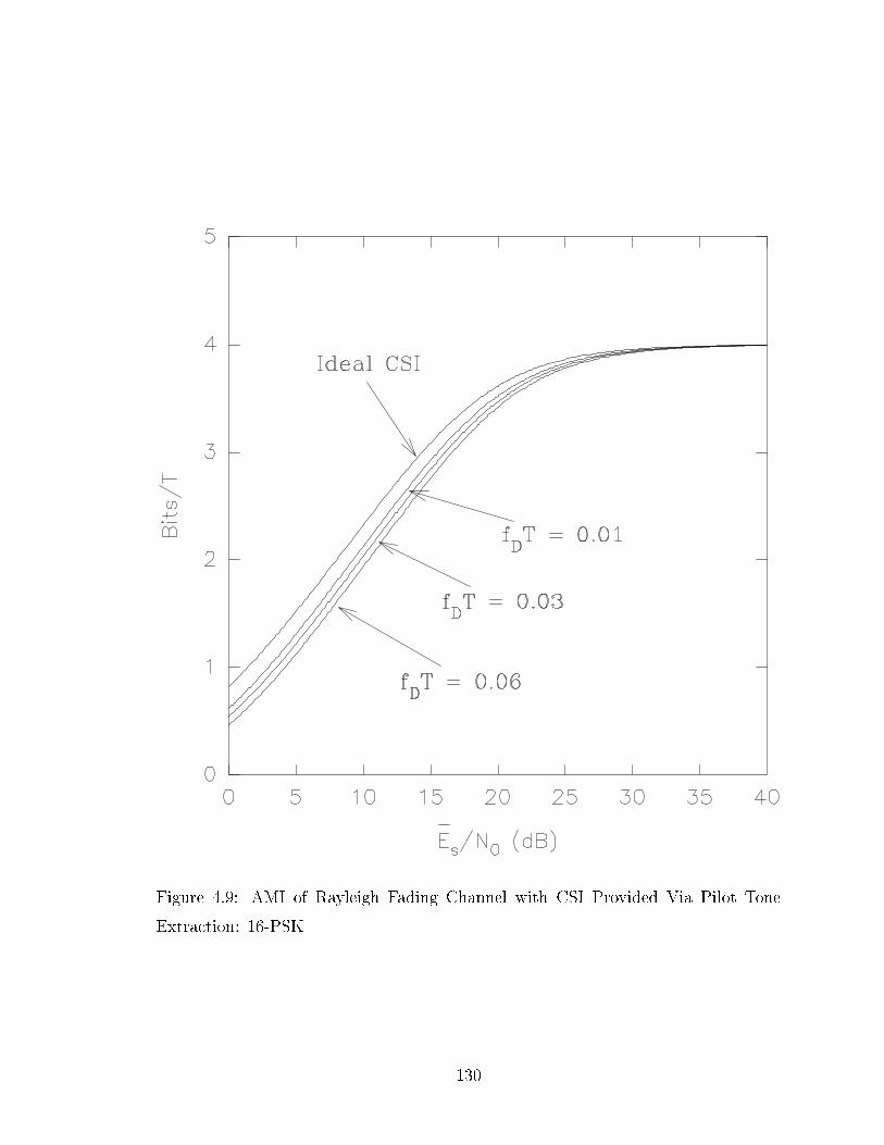
Figure 4.9: AMI of Rayleigh Fading Channel with CSI Provided Via Pilot Tone
Extraction: 16-PSK
130

Figure 4.10: AMI of Rayleigh Fading Channel with CSI Provided Via Pilot Tone
Extraction: 16-QAM
131
Figure 4.11: AMI of Rayleigh Fading Channel with CSI Provided Via Pilot Tone
Extraction: 32-CR
132

fDT = 0:01 fDT = 0:03 fDT = 0:06
8-PSK 16-PSK 8-PSK 16-PSK 8-PSK 16-PSK
3.5 - 1.1 dB - 1.7 dB - 2.2 dB
3 - 1.1 dB - 1.7 dB - 2.2 dB
AMI 2.5 1.2 dB 1.1 dB 1.8 dB 1.7 dB 2.2 dB 2.3 dB
(Bits/T ) 2 1.2 dB 1.2 dB 1.8 dB 1.8 dB 2.3 dB 2.4 dB
1.5 1.4 dB 1.3 dB 1.9 dB 1.9 dB 2.6 dB 2.4 dB
1 1.5 dB 1.5 dB 2.1 dB 2.1 dB 2.8 dB 2.8 dB
Table 4.4: Loss of SNR Due to Non-Ideal CSI: Pilot Tone Estimation with PSK
Constellations
to the ideal case corresponding to an increase in Doppler frequency. The magnitude
of the loss compared to a fading channel with ideal CSI is stated for various values of
AMI in Table 4.4 for the PSK constellations, and in Table 4.5 for the case of when
QAM signal sets are used. When a 2k-point signal set is considered for data rates in
the range of 1 to k � 0:5 bits/T , the loss for a normalized Doppler frequency of 0.01
is in the range of 1 to 1.5 dB. As the Doppler frequency increases to 0.03 so does the
loss, which takes on values in the range of 1.5 to 2 dB. For a fDT of 0.06, the loss
compared to the ideal case is in the range of 2 to 2.8 dB.
Although the results presented here indicate that pilot tone extraction is a promis-
ing method of channel state estimation, in practice it is not a very popular method
to use. One reason is due to the extra complexity necessary to transmit and extract
the pilot tone. Another reason is the requirement of shaping the spectrum in order to
create a null for the placement of the pilot tone. As a solution to this second problem,
a method which utilizes two pilot tones placed at the edges of the transmit band is
considered in [57] for use in mobile satellite communications.
4.3.2 Channel Estimation Via Di�erentially Coherent Detec-
tion
Di�erentially coherent detection combined with DPSK modulation is commonly used
in fading environments where time variation of the channel makes estimation of the
133

fDT = 0:01 fDT = 0:03 fDT = 0:06
16-QAM 32-CR 16-QAM 32-CR 16-QAM 32-CR
4.5 - 1.0 dB - 1.5 dB - 2.0 dB
4 - 1.0 dB - 1.5 dB - 2.0 dB
3.5 1.1 dB 1.1 dB 1.6 dB 1.6 dB 2.1 dB 2.1 dB
AMI 3 1.1 dB 1.1 dB 1.6 dB 1.6 dB 2.1 dB 2.1 dB
(Bits/T ) 2.5 1.1 dB 1.1 dB 1.7 dB 1.6 dB 2.1 dB 2.1 dB
2 1.2 dB 1.2 dB 1.8 dB 1.7 dB 2.2 dB 2.2 dB
1.5 1.2 dB 1.2 dB 1.8 dB 1.8 dB 2.3 dB 2.3 dB
1 1.4 dB 1.5 dB 2.0 dB 2.1 dB 2.6 dB 2.7 dB
Table 4.5: Loss of SNR Due to Non-Ideal CSI: Pilot Tone Estimation with QAM
Constellations
134

carrier phase diÆcult. This signalling method can also be viewed as a scheme which
provides information about the fading variable �. Only PSK constellations are dealt
with here, although di�erential encoding of the phase of multi-level constellations has
also been considered [58].
Let xi denote a symbol from a PSK constellation. It is assumed here that the
amplitude is normalized so that jxij = 1. The process of di�erentially encoding the
phase of the channel symbol can be interpreted as a multiplication of two complex
numbers. The di�erentially encoded symbol during the ith transmission interval is
xi = xi�1xi (4.61)
where xi is the PSK symbol to be transmitted during the ith signalling interval, and
xi�1 is the di�erentially encoded symbol transmitted during the previous interval.
During transmission, the symbol xi is a�ected by fading and further corrupted by
additive noise. The received channel symbol is
yi = �ixi + ni: (4.62)
Substituting equation (4.61) into equation (4.62) yields
yi = �ixi�1xi + ni: (4.63)
In this case, it is desired to estimate the quantity �ixi�1. On examination of equation
(4.62), it is observed that yi�1 can serve as a noisy estimate of �ixi�1. Therefore, the
channel state estimate for �ixi�1 is
~�i = �i�1xi�1 + ni�1: (4.64)
The variance of the estimate ~�i is given by 12Enj~�ij2
o, and can be shown to equal
�2~� = �2� + �2N : (4.65)
The quantity 12En�i
~��iois equal to R�(T )x
�i�1, where R�(T ) is the autocorrelation
function of the fading process evaluated for a time di�erence of the channel symbol
duration T . For land mobile radio, the autocorrelation function is modelled by the
equation [29]
R�(�) = �2�J0(2�fD�) (4.66)
135

where fD is the Doppler frequency, and J0(�) is a Bessel function of the �rst kind
and of zero order. Using this result in equation (4.55) allows one to calculate the
squared magnitude of the correlation coeÆcient between the fading variable � and
the estimate ~� to be
j�j2 = J20 (2�fDT )
1 +�
�EsN0
��1 (4.67)
where�EsN0
is de�ned here to equal�2��2N
.
The required parameters necessary to evaluate equation (4.54) have been deter-
mined. However, this expression for AMI can be somewhat simpli�ed. Since it is
assumed that PSK constellations are used, the magnitude jxij of the channel symbolsis the same for all points of the constellation for the system under consideration. It
is also assumed in this case that jxij = 1 for all i. Using this fact, the expression for
AMI can be simpli�ed to
I(X;Y j~�) = log2M� (4.68)
1
M
MXi=1
Ep(�;~�)p(n)
8<:log2
24 MXj=1
exp
0@ j�xi + n� ���~�xi
�~�j2 � j�xi + n� ���~�xj
�~�j2
2[(1� j�j2)�2� + �2N ]
1A359=; :
This expression for AMI was evaluated by means of computer simulation for two
levels of PSK constellation. Results for an 8-PSK signal set are shown in Figure 4.12,
while Figure 4.13 contains the curves for 16-PSK. Three di�erent values were con-
sidered for the normalized Doppler frequency fDT . These values are 0.01, 0.03, and
0.06. On examination of the AMI curves, it is evident at low values of SNR that
the loss is mostly due to the noise term added to the estimate. As the SNR gets
larger, the signi�cant e�ect is due to Doppler spread. As the Doppler frequency in-
creases, the maximum achievable AMI decreases noticeably from a value of log2M .
For normalized Doppler frequencies of 0.01, 0.03, and 0.06, the AMI curves for 8-PSK
reach maximum values of approximately 2.97, 2.80, and 2.36 bits/T , respectively.
The respective values of maximum AMI for the case of 16-PSK are 3.90, 3.38, and
2.35 bits/T . The loss in SNR required for error free transmission compared to the
ideal CSI case is shown in Table 4.6 for various rates of average mutual information.
Considering rates in the range of 1 to k � 0:5 bits/T using a 2k-point constellation,
and a Doppler frequency of fDT = 0:01, the loss is roughly 3.2 to 3.7 dB. When
136

Figure 4.12: AMI of Rayleigh Fading Channel with CSI Provided Via Di�erentially
Coherent Detection: 8-PSK
137

Figure 4.13: AMI of Rayleigh Fading Channel with CSI Provided Via Di�erentially
Coherent Detection: 16-PSK
138

fDT = 0:01 fDT = 0:03 fDT = 0:06
8-PSK 16-PSK 8-PSK 16-PSK 8-PSK 16-PSK
3.5 - 3.7 dB - - - -
3 - 3.3 dB - 6.0 dB - -
AMI 2.5 3.3 dB 3.2 dB 4.9 dB 4.3 dB - 16.2 dB
(Bits/T ) 2 3.2 dB 3.2 dB 3.8 dB 3.8 dB 6.4 dB 6.2 dB
1.5 3.4 dB 3.3 dB 3.6 dB 3.6 dB 4.7 dB 4.7 dB
1 3.7 dB 3.7 dB 3.8 dB 3.8 dB 4.3 dB 4.3 dB
Table 4.6: Loss of SNR Due to Non-Ideal CSI: Di�erentially Coherent Detection with
PSK Constellations
139

fDT = 0:03, the losses are in the range of 3.6 to 4.9 dB for 8-PSK, and from 3.6 to
6.0 dB for 16-PSK. For a normalized Doppler frequency of 0.06, the loss for 8-PSK is
roughly 4.3 to 6.4 dB, while the 16-PSK results show a loss in the range of 4.3 to 16.2
dB. Although the use of di�erential detection is much simpler to implement than the
use of a pilot tone, the performance of the resulting communication system is much
more sensitive to frequency dispersive e�ects.
4.3.3 Channel Estimation Via Pilot Symbol Transmission
As a �nal method of obtaining an estimate of the fading process of the channel, the
transmission of a pilot symbol along with the data is considered. This method is
simple in concept. For a block of NB signalling intervals, the �rst transmission is a
known pilot symbol xp. Since this symbol is known at the receiver, it allows a noisy
estimate of the fading variable � to be obtained during the �rst signalling interval of
the block. This estimate is then used to approximate the fading variable for the next
NB � 1 received channel symbols. The channel estimate for a block of size NB is
~� = �xp + n: (4.69)
A complication arises in analyzing this method of channel estimation, in that
the model parameters are dependent upon the time delay between when the pilot
symbol is transmitted and when the channel estimate is used. For the moment this
consideration will be ignored, and the correlation coeÆcient between the estimate
and the fading variable is determined as a function of the delay. Suppose the fading
estimate is used l symbol intervals after it is obtained. The term 12En�l
~��ois
calculated to be x�pR�(lT ), where R�(lT ) is the autocorrelation function of the fading
process evaluated for a time di�erence of lT . The Bessel function model stated in
equation (4.66) for the case of di�erential detection will be used again here. Assuming
the pilot symbol to have an amplitude A, the quantity 12Enj~�j2
ois determined to
be equal to �2�A2 + �2N . Using these facts in conjunction with equation (4.55), the
squared magnitude of the correlation coeÆcient between the channel estimate ~� and
140

the fading variable � at a time of lT symbol intervals later is determined to be
j�lj2 = J20 (2�lfDT )
1 +�2N
�2�A2
: (4.70)
Let EX be the average energy of those symbols carrying information. De�ne the
parameter = A2
(NB�1)EX to be the ratio of the energy used in the pilot symbol to
that used in the data portion of the transmission. If Es is the average energy per
symbol of a block of NB symbols, of which one is a pilot symbol and the other are
data symbols, it is a simple matter to show that
A2 = NB
1 + Es: (4.71)
By using this in equation (4.70), the squared norm of the correlation coeÆcient is
expressed as
j�lj2 = J20 (2�lfDT )
1 +�1+ NB
� ��EsN0
��1 (4.72)
where�EsN0
=�2�Es�2N
. The variance �2~� is simply equal to �2�A2 + �2N , as shown above.
Using the result in (4.71), and the assumption that the average symbol energy is
normalized so that Es = 1, this variance can be determined from the equation
�2~� =
NB
1 +
!�2� + �2N : (4.73)
All that needs to be dealt with is the time variation of the model. In order to do
this, the AMI will be considered as an average over long sequences of symbols. The
de�nition of average mutual information can be expressed as
I(X;Y j~�) = lim�!1
1
�NB[H(X�NB)�H(X�NB jY�NB ; ~��NB)] (4.74)
where, for example, X�NB represents a sequence of �NB symbols Xl. Under the
assumption of ideal interleaving, a memoryless channel model is obtained, and the
expression in (4.74) can be written
I(X;Y j~�) = lim�!1
1
�NB
24�NBXl=1
I(Xl;Ylj~�l)
35= lim
�!11
�NB
24�NBXl=1
H(Xl)��NBXl=1
H(XljYl; ~�l)
35 :
(4.75)
141

For a block of �NB symbols, the additive terms in equation (4.75) may be divided
into groups of size �. In e�ect, this can be viewed as an average over NB parallel
channels. One of these channels will be used for the transmission of the pilot symbol
xp. Since xp is known, the AMI over this particular channel is zero. For each of
the other parallel channels, the AMI between Xl and Yl conditioned on ~�l may be
determined, where the delay between the fading variable and the estimate is lT . This
allows the AMI to be expressed
I(X;Y j~�) = lim�!1
1
NB
"NXl=1
I(Xl;Ylj~�l)
#=
1
NB
NB�1Xl=1
hH(Xl)�H(XljYl; ~�l)
i: (4.76)
Assuming an equiprobable input distribution, and using the expression forH(XjY; ~�)stated in equation (4.53), the AMI for a channel in which the fading estimate is
obtained through pilot symbol transmission is determined to be
I(X;Y j~�) = NB � 1
NBlog2M� (4.77)
1NBM
PNB�1l=1
PMi=1E
(log2
"PMj=1
[(1�j�lj2)jxij2�2�+�2N ]
[(1�j�lj2)jxj j2�2�+�2N ]exp
j�xi+n��l��~�xi
�~�j2
2[(1�j�lj2)jxij2�2�+�2N ]
� j�xi+n��l��~�xj
�~�j2
2[(1�j�lj2)jxj j2�2�+�2N ]
1A359=; :
The expression for AMI in equation (4.77) was evaluated for a number of di�erent
cases. The constellations considered were 8-PSK and 16-QAM, and the AMI curves
for these signal sets are contained in Figure 4.14 and Figure 4.15, respectively. The
same values of normalized Doppler frequency were considered as for the previous
methods of channel estimation, namely fDT taking on values of 0.01, 0.03, and 0.06.
A block size of NB = 5 was chosen for analysis. This value was used in [59] in
combination with TCM for transmission over a Rician fading channel. An optimum
value of the parameter exists for a given value of NB. In general, as long as jxpj2is of the order of EX , the AMI is essentially near the maximum value. A slight
improvement occurs when jxpj2 = 2EX or more, and a value of = 0:5 was used in
the simulations performed because of this. If jxpj2 is made extremely large, then the
AMI will start to decrease due to the fact that most of the energy is being used to
transmit the pilot symbol rather than the data.
142

Figure 4.14: AMI of Rayleigh Fading Channel with CSI Provided Via Pilot Symbol
Transmission: 8-PSK
143

Figure 4.15: AMI of Rayleigh Fading Channel with CSI Provided Via Pilot Symbol
Transmission: 16-QAM
144

fDT = 0:01 fDT = 0:03 fDT = 0:06
8-PSK 16-QAM 8-PSK 16-QAM 8-PSK 16-QAM
2.5 - 7.2 dB - - - -
AMI 2 8.3 dB 5.5 dB - 11.5 dB - -
(Bits/T) 1.5 5.7 dB 4.8 dB 10.7 dB 7.1 dB - -
1 5.0 dB 4.5 dB 6.6 dB 5.7 dB 27.3 dB 10.3 dB
Table 4.7: Loss of SNR Due to Non-Ideal CSI: Pilot Symbol Transmission
The results for pilot symbol detection indicate that the losses are quite severe
compared to other estimation methods, and the e�ect of Doppler spread is clear. The
maximum achievable AMI tends to a value which is signi�cantly less than log2M
bits/T for a M -point constellation. For a normalized Doppler frequency fDT of 0.01,
the 8-PSK results tend to a value of 2.27 bits/T , while the 16-QAM curve levels
out at 2.99 bits/T . As the Doppler frequency increases to 0.03, the AMI is limited
to approximately 1.70 bits/T for 8-PSK, and 2.21 bits/T for 16-QAM. Maximum
values of 1 bit/T and 1.36 bits/T are reached for a normalized Doppler frequency of
0.06 using 8-PSK and 16-QAM, respectively. Table 4.7 contains the loss in required
SNR for error free transmission compared to the ideal CSI case when pilot symbol
transmission is used. These losses are quite large, and indicate the sensitivity of the
channel estimation method to Doppler e�ects. Additional simulations were performed
in order to determine the best value ofNB for a given value of fDT . When fDT = 0:01,
values of NB in the range of 5 to 8 yield comparable results. When fDT = 0:03, a
block length NB set to 4 yields the best result. For fDT = 0:06, a value of NB = 3
yields the best result. By choosing NB = 3 when fDT = 0:06, the maximum AMI
can be increased by approximately 0.3 bits/T compared to the results presented here
for NB = 5.
Pilot symbol transmission was considered in [59] and [60] for use in combination
with TCM. The results presented indicate that this method is promising when a
LOS component exists. Results presented here indicate that for a Rayleigh channel,
this method is only good for systems which experience small amounts of frequency
dispersion.
145

Chapter 5
Information Theoretic Bounds for
Frequency-Selective Fading Channels
When the e�ects of time dispersion on the performance of a communication system
become prominent, a fading channel is more accurately modelled as being frequency-
selective. In this chapter, the e�ect of time dispersion on the rate of reliable data
communication is investigated through calculation of information theoretic quantities
for frequency-selective fading channels. A signi�cant di�erence in comparison to the
at fading case is that rather than considering only channel symbols, the actual wave-
forms used for communication must be taken into account when performing analysis.
As a basis for the results presented here, a de�nition of average mutual information
and capacity for waveform channels is discussed �rst. The two-path Rayleigh fading
model is used here to account for the e�ect of time dispersion on communication.
Following an examination of the properties of the two-path model, the capacity of a
bandlimited frequency-selective Rayleigh fading channel is determined.
For certain cases of frequency-selective fading, the channel exhibits a time diversity
e�ect. Since the use of diversity usually in uences the performance of a communica-
tion system in a positive manner, the e�ect of this time diversity on the achievable
rate of reliable data transmission is determined for channels with discrete-valued in-
put. This is accomplished through calculation of the average mutual information of
the channel. Channels with continuous-valued input are also considered, and limits
on communication rate are likewise determined.
146

5.1 Representation of Waveform Channels
The channel models considered up to now have been discrete with respect to the
variable of time. For such channels, the statistical behavior of a random signal is de-
scribed by a joint probability distribution de�ned at speci�c instants of time, usually
at equally spaced intervals of the channel symbol duration T . When time dispersion
is present in a communication medium, the energy associated with any given trans-
mitted symbol is spread out over more than just the original pulse duration. Even
when the output of the channel is sampled at intervals of T seconds, the received
symbol is also dependent upon the behaviour of the transmitted signal between sam-
pling instants. Due to this eventuality, the waveforms chosen for communication play
an important role in determining the performance of the system. Thus, any analytic
model which is applied must be based on waveform channels which are continuous
with respect to time.
The �rst problem encountered for such a model is in de�ning the probability
of a continuous waveform. In order to completely describe the stochastic behavior
of a random process, a rule is required which allows the speci�cation of a joint pdf
describing the process observed at any given �nite set of times. An alternate solution,
which is more bene�cial analytically, is to represent signals by a series expansion of
a set of orthonormal waveforms. If a waveform can be completely speci�ed by such a
series, then the signal can be characterized by a joint pdf over the coeÆcients of the
expansion. For example, suppose that any given waveform x(t) from a particular set
X(t) de�ned over the time interval (0; Ts) can be uniquely represented in the form
x(t) =1Xi=1
xi'i(t) (5.1)
where the 'i(t) are a set of orthonormal functions, and the xi are coeÆcients of
the series expansion. Such a family of waveforms can be described for the �rst NB
values of xi by the joint pdf p(x1; : : : ; xNB). If this joint pdf were to completely specify
each waveform in the set, then the class of functions would be described as having NB
degrees of freedom. It is assumed that any sample function y(t) of the channel output
process Y (t) can also be uniquely expanded into a series of orthonormal functions
147

given by
y(t) =1Xi=1
yi'i(t) (5.2)
where the 'i(t) are a set of orthonormal functions which are not necessarily the same
as the set of 'i(t). If the statistics of the �rst NB coeÆcients of this expansion are
described by the joint pdf p(y1; : : : ; yNB), then one may de�ne the AMI between the
two continuous-time random processes X(t) and Y (t) to be
I(X(t);Y (t)) = limNB!1
�Ep(x1;:::;xNB ;y1;:::;yNB )
(log
p(x1; : : : ; xNB ; y1; : : : ; yNB)
p(x1; : : : ; xNB)p(y1; : : : ; yNB)
!):
(5.3)
Using this de�nition of AMI, the capacity of the channel per unit time can then be
de�ned as
C = limTs!1
1
Tssup I(X(t);Y (t)) (5.4)
where the supremum is taken over all possible sets of input waveforms which can be
described by the series expansion. If such a value of C exists, then the information
rate must be kept less than C in order to attain an arbitrary degree of reliability.
In addition, it is noted that examples of channels can be constructed for which such
a value of C exists, but for which arbitrarily low probability of transmission error
cannot be realized at rates below C [27].
Such a model for a continuous-time channel can easily be made mathematically
unstable with regard to convergence of series, uniqueness of the series expansion,
and modelling of the additive noise process. In order to circumvent these problems,
certain constraints are often imposed upon the system. Fortunately, the type of
restrictions imposed to stabilize the model are not arti�cial in nature, but re ect
practical constraints which are encountered in actual communication systems. The
usual constraints assumed to be placed on the system are a �nite limit on the value
of transmitted energy or average power, as well as limits on the time duration of the
signal and the bandwidth of the system.
In order to allow the expansion of a random process into a series of orthonormal
functions, any sample function x(t) of the process X(t) under consideration can usu-
ally be formulated in a manner that allows it to be categorized as being a L2 function.
148
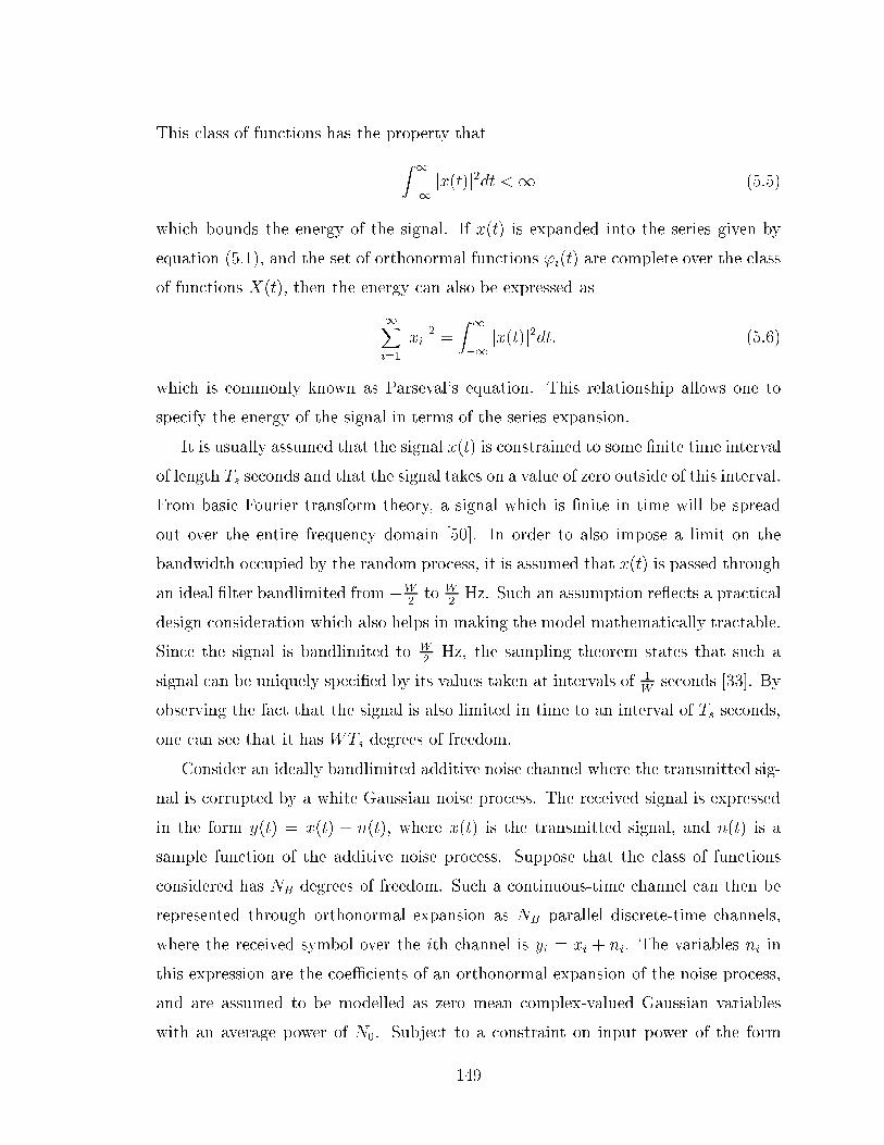
This class of functions has the property that
Z 1
�1jx(t)j2dt <1 (5.5)
which bounds the energy of the signal. If x(t) is expanded into the series given by
equation (5.1), and the set of orthonormal functions 'i(t) are complete over the class
of functions X(t), then the energy can also be expressed as
1Xi=1
jxij2 =Z 1
�1jx(t)j2dt: (5.6)
which is commonly known as Parseval's equation. This relationship allows one to
specify the energy of the signal in terms of the series expansion.
It is usually assumed that the signal x(t) is constrained to some �nite time interval
of length Ts seconds and that the signal takes on a value of zero outside of this interval.
From basic Fourier transform theory, a signal which is �nite in time will be spread
out over the entire frequency domain [50]. In order to also impose a limit on the
bandwidth occupied by the random process, it is assumed that x(t) is passed through
an ideal �lter bandlimited from �W2to W
2Hz. Such an assumption re ects a practical
design consideration which also helps in making the model mathematically tractable.
Since the signal is bandlimited to W2Hz, the sampling theorem states that such a
signal can be uniquely speci�ed by its values taken at intervals of 1W
seconds [33]. By
observing the fact that the signal is also limited in time to an interval of Ts seconds,
one can see that it has WTs degrees of freedom.
Consider an ideally bandlimited additive noise channel where the transmitted sig-
nal is corrupted by a white Gaussian noise process. The received signal is expressed
in the form y(t) = x(t) + n(t), where x(t) is the transmitted signal, and n(t) is a
sample function of the additive noise process. Suppose that the class of functions
considered has NB degrees of freedom. Such a continuous-time channel can then be
represented through orthonormal expansion as NB parallel discrete-time channels,
where the received symbol over the ith channel is yi = xi + ni. The variables ni in
this expression are the coeÆcients of an orthonormal expansion of the noise process,
and are assumed to be modelled as zero mean complex-valued Gaussian variables
with an average power of N0. Subject to a constraint on input power of the form
149

EnR Ts
0 jx(t)j2dto� PTs, the average power of the discrete-time symbols xi can be de-
rived from equation (5.6) to be PTsNB
, where it is assumed that the power is distributed
equally among the parallel channels. The capacity for each parallel channel is
Ci = log�1 +
PTsNBN0
�bps=Hz (5.7)
which is the classical result for a discrete-time AWGN channel. By adding the con-
tributions from each individual parallel channel, the total capacity per unit time of
the waveform channel is determined to be
C =NB
Tslog
�1 +
PTsNBN0
�bps: (5.8)
Since it is assumed that the signal is bandlimited to W2Hz and time limited to Ts
seconds, the class of signals has NB = WTs degrees of freedom, and equation (5.8)
becomes
C =W log�1 +
P
WN0
�bps (5.9)
which is the capacity of an ideal bandlimited AWGN channel.
For more on the modelling of waveform channels, see [27], which contains more
mathematical detail as well as references to works which deal with some of the prob-
lems encountered with this model.
5.1.1 Time-Invariant Filter Channels
While the assumption of an ideally at transfer characteristic for a channel re ects
the imposed bandwidth constraint, the response of any real channel will likely not
be at across all frequencies in the transmit bandwidth. A more accurate model of
a bandlimited channel would include an arbitrary transfer characteristic. In order to
accomplish this, the response of the channel can be modelled as a linear time-invariant
�lter. Based on this idea, the channel can be represented so that the output signal is
y(t) =Zx(�)h(t� �)d� + n(t) (5.10)
where x(t) is the transmitted signal, h(t) is the impulse response of the �lter describing
the channel, and n(t) is a sample function of the additive noise process. It is also
assumed that the input is limited in time to a duration of Ts seconds and has an
150
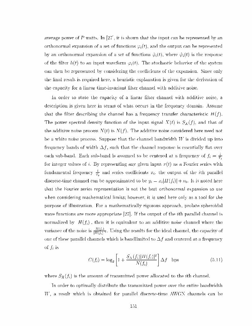
average power of P watts. In [27], it is shown that the input can be represented by an
orthonormal expansion of a set of functions 'i(t), and the output can be represented
by an orthonormal expansion of a set of functions 'i(t), where 'i(t) is the response
of the �lter h(t) to an input waveform 'i(t). The stochastic behavior of the system
can then be represented by considering the coeÆcients of the expansion. Since only
the �nal result is required here, a heuristic explanation is given for the derivation of
the capacity for a linear time-invariant �lter channel with additive noise.
In order to state the capacity of a linear �lter channel with additive noise, a
description is given here in terms of what occurs in the frequency domain. Assume
that the �lter describing the channel has a frequency transfer characteristic H(f).
The power spectral density function of the input signal X(t) is SX(f), and that of
the additive noise process N(t) is N(f). The additive noise considered here need not
be a white noise process. Suppose that the channel bandwidth W is divided up into
frequency bands of width �f , such that the channel response is essentially at over
each sub-band. Each sub-band is assumed to be centered at a frequency of fi =iTs
for integer values of i. By representing any given input x(t) as a Fourier series with
fundamental frequency 1Ts
and series coeÆcients xi, the output of the ith parallel
discrete-time channel can be approximated to be yi = xijH(fi)j+ni. It is noted here
that the Fourier series representation is not the best orthonormal expansion to use
when considering mathematical limits; however, it is used here only as a tool for the
purpose of illustration. For a mathematically rigorous approach, prolate spheroidal
wave functions are more appropriate [27]. If the output of the ith parallel channel is
normalized by jH(fi)j, then it is equivalent to an additive noise channel where the
variance of the noise is N(fi)jH(fi)j2 . Using the results for the ideal channel, the capacity of
one of these parallel channels which is bandlimited to �f and centered at a frequency
of fi is
C(fi) = log2
"1 +
SX(fi)jH(fi)j2N(fi)
#�f bps (5.11)
where SX(fi) is the amount of transmitted power allocated to the ith channel.
In order to optimally distribute the transmitted power over the entire bandwidth
W , a result which is obtained for parallel discrete-time AWGN channels can be
151

used [27, p. 343]. The optimal distribution of power over all bands is
SX(fi) =
8><>:K0 � N(fi)
jH(fi)j2 for i 2 IW0 for i =2 IW
(5.12)
where IW =ni j fi 2 W; N(fi)
jH(fi)j2 < K0
o, and K0 is chosen so that
Pi2IW SX(fi) = P .
By using this result along with equation (5.11), the capacity of a channel with an
arbitrary �lter response is approximated to be
C � Xi2IW
log
"K0jH(fi)j2N(fi)
#�f: (5.13)
By letting �f ! 0, this discrete approximation becomes continuous in the limit, and
the capacity of a �lter channel with noise is determined to be
C =Zf2FW
log
"K0jH(f)j2N(f)
#df (5.14)
where FW =nf 2 W j N(f)
jH(f)j2 < K0
o, and the level K0 is set so that the total trans-
mitted power is limited toRf2FW SX(f)df = P . The power spectral density of the
capacity achieving input is
SX(f) =
8><>:K0 � N(f)
jH(f)j2 for f 2 FW0 for f =2 FW
: (5.15)
This distribution of the input power is often given a \water-�lling" interpretation.
The meaning of this statement can be explained as follows. If the function N(f)jH(f)j2 is
considered to be the bottom of a vessel, and an amount P of water is poured into this
vessel, the liquid would naturally be distributed in a manner described by equation
(5.15). If it is assumed that jH(f)j = 1 over the band from �W2
to W2
and zero
elsewhere, and that the noise is white with a constant power spectral density of N0,
then application of equation (5.14) would yield the result shown in equation (5.9) for
the ideal �lter channel.
5.2 Capacity of the Two-Path Rayleigh Channel
It would be nice if the results obtained for the time-invariant �lter case could also be
used for time-varying channel responses. In [27], mathematical development of the
152

orthonormal expansion of functions does not depend on the time-invariance of the
�lters. In fact, time-varying �lters are used in the model in order to limit the time
duration of strictly bandlimited signals. In order to use these known results, a number
of assumptions are made here. Suppose that the time-varying �lter can be described
stochastically by some type of probability distribution p(h(t)). The term p(h(t)) is
used to denote the general statistics of the random process h(t). If it is possible for
this response to be determined, then a conditional AMI I(X(t);Y (t)jh(t)) can be
de�ned. Since h(t) is assumed to always be known, this AMI can be determined for
a �xed response of h(t), then averaged over the statistics describing h(t) in order to
determine the conditional AMI.
The two-path Rayleigh channel is described by the impulse response
h(t) = �1(t)Æ(t) + �2(t)Æ(t� �) (5.16)
and is completely speci�ed by �1(t), �2(t), and � . The usual complex-valued fading
variables are written here as random processes in order to illustrate the time-varying
nature of the channel. Since � is assumed to be �xed, the desired quantity to be
determined is I(X(t);Y (t)j�1(t);�2(t)). In order to achieve capacity, given the value
of �1(t) and �2(t) at any �xed time, the spectrum of the input should be that achieved
by the water pouring argument stated in the previous section. As time progresses and
�1(t) and �2(t) change, the spectrum should also be adjusted in order to maintain the
water pouring characteristic. Since no other spectrum results in a greater AMI, this
result yields the capacity of the channel. The assumption that �1(t) and �2(t) are
always known is equivalent to having ideal CSI. In a practical system, this assumption
may be realized by an equalizer which is able to track changes in the channel.
If the response of a time-varying channel is always known, then the capacity may
be determined. In order to obtain actual numbers, however, one must overcome the
diÆculty of averaging over the statistics of h(t). It would be nice if the problem could
be formulated in the same manner as was done for the time-invariant case, in which
random channel responses could be generated and the capacity could be determined
for each �xed response. The capacity could then be obtained from the average of
these results. It is reasonable to assume that h(t) is an ergodic random process and
that the time average is the same as the ensemble average taken with respect to
153

the variables �1 and �2. This could be used to verify the results mathematically.
Rather than attempting this diÆcult approach, a more practical argument is used
here. Another way of looking at this situation is by implementing the assumption of
perfect interleaving. Let the transmitted waveform be represented as
x(t) =Xi
xi(t) (5.17)
where the xi(t) are pulses which are transmitted every T seconds. These pulses
need not be �nite in duration, although this is necessarily the case for a real system.
It is reasonable to believe that if the xi(t) are L2 functions and overlap of these
functions does not cause the the signal to become unbounded, then the signal may
be represented in this manner. If ideal interleaving is used, then at the receiver
these pulses look as though they were a�ected by independent channel responses.
The main point here is that in order to perform averaging over the statistics of the
channel response, one may randomly generate values of �1 and �2 and perform a water
pouring of signal energy for each given channel. The average result of this random
water pouring yields the capacity of the channel.
5.2.1 Properties of the Two-Path Model
In order to apply the water pouring of signal energy to randomly generated channel
responses, there are certain obstacles to overcome. For each randomly generated
channel response, the band of frequencies FB over which the signal spectrum is non-
zero as well as the parameter K0 are variable. This makes it diÆcult to develop an
algorithm to evaluate the capacity through computer simulation.
Fortunately, the two-path model has a high degree of symmetry, and parameters
which are easily calculated from the given values of �1, �2, and � . It is assumed that
the additive noise is a white noise process with a constant power spectral density of
N0 over the bandwidth of interest. The channel SNR function is jH(f)j2N0
, and it is
the inverse of this quantity into which the signal energy is poured. For the two-path
Rayleigh channel, this is
G(f) =N0
�1 + �2 cos 2��f + �3 sin 2��f(5.18)
154

where �1 = j�1j2 + j�2j2, �2 = 2<f�1��2g, and �3 = �2=f�1��2g. The function G(f)is periodic with period ��1. By di�erentiating G(f) with respect to f , the critical
points are determined to occur at
fcrit =1
2��arctan
�3
�2+
i
2�(5.19)
where i is an integer. The value of �2 speci�es whether the value obtained with i = 0
results in a maximum or minimum value of G(f). If �2 is positive, then the maximum
points occur at values of fmax =1
2��arctan �3
�2+ i
�and the minimum points occur at
fmin = 12��
arctan �3�2
+ i�+ 1
2�. If �2 should happen to be negative, then the roles
of fmax and fmin stated here are reversed. The maximum value taken on by G(f) is
N0
j�1j2+j�2j2�2j�1jj�2j , and the minimum value is N0
j�1j2+j�2j2+2j�1jj�2j . This information about
G(f) can be used to create an algorithm to optimally distribute the signal spectrum
for a randomly generated G(f).
In order to perform a computer simulation, the total power of the signal is assumed
to be set to P = 1. The SNR is then determined by the value of the noise power
WN0, whereW2is the bandwidth of the channel. The channel responses are obtained
by randomly generating values of �1 and �2. The delay spread � is chosen to equal
some �xed value. The channel is strictly bandlimited from �W2
to W2
Hz. The
capacity achieving spectrum for a given channel response can be determined as follows.
Since the maximum value of N0
jH(f)j2 can be easily determined, the parameter K0 can
initially be set to this value. IfR W
2
�W2
K0� N0
jH(f)j2df is less than 1, then K0 is chosen to
equal 1W
�1 +
R W2
�W2
N0
jH(f)j2df�, and the set of frequencies FW is the entire bandwidth.
By applying equation (5.14), the capacity conditioned on �1 and �2 is determined
through numerical integration. If setting K0 to the maximum value of N0
jH(f)j2 results
inR W
2
�W2
K0 � N0
jH(f)j2df > 1, then the transmit spectrum must be broken up, and
FW is no longer a continuous set of frequencies. The �rst step is to determine the
location of the maximum points within the bandwidth, as well as the two maxima just
outside either band edge. A bisection algorithm can then be applied to the range of
frequencies between maxima. For each iteration, a new range of FW and value of K0
is determined, and the resulting total average power is reevaluated. This is continued
until the total transmit power is suÆciently close to 1. When this is accomplished, a
155

�nal value of K0 is determined as well as the set of frequencies FW . This is then used
to evaluate equation (5.14).
5.2.2 Capacity and Equalization
The random water pouring algorithm was performed for various values of delay spread
and power distribution between the individual paths of the model. In all cases, the
capacity was equivalent to that of an ideal Rayleigh fading channel. Only a minor
variation occurred at low values of SNR.
Such a consequence might have been guessed by applying Price's result. In [61],
he showed that the capacity of an arbitrary linear �lter channel with additive noise
is the same at high SNR as an ideal �lter channel. In addition, it was shown that
the capacity could be realized at high SNR by adaptive equalization as performed
through the use of precoding or decision feedback equalization. By extending these
results to the case of a fading channel, the capacity for any given �lter response is
determined to be the same as that of a channel with a at transfer characteristic. The
only di�erence is the varying level of attenuation of the equalized channel. Averaging
over randomly generated �lters yields the result for the at fading channel. As long
as variations in the channel can be tracked, use of decision feedback equalization or
precoding should place the capacity of a frequency-selective channel at no more that
2.51 dB from the capacity of an ideal AWGN channel, which is the loss due to fading
experienced by an ideal Rayleigh channel.
5.3 Time Diversity E�ect
One of the drawbacks of the waveform channel model used in the previous section
is that the channel output resulting from a given input of duration Ts is restricted
to be observed over essentially the same length of time. As a consequence of this
model characteristic, the e�ect of intersymbol interference between channel symbols
is essentially ignored. As was mentioned previously, a time diversity e�ect sometimes
manifests itself when time dispersion is present on the channel. In order to analyze
the e�ects of this time diversity, it is necessary to think in terms of discrete signalling
156
intervals. Partitioning the time continuum in this manner allows one to determine
the e�ect that a waveform transmitted during a given interval has on the waveform
observed during subsequent intervals at the receiver.
A particular class of signalling waveforms is investigated here in order to illustrate
the e�ect of this inherent time diversity on the rate of reliable data transmission. In
order to partition the continuous waveform into discrete signalling intervals, the �rst
assumption made is that channel symbols are transmitted at a rate of one symbol
every T seconds, and that received channel symbols are obtained by sampling the
output of the waveform channel at the same rate. This is a reasonable assumption to
make in that any practical system can be viewed at certain points as being discrete
in time. The joint probability distribution between the input and output symbol se-
quences, however, is still dependent upon the continuous-time waveform channel. The
second assumption made is that the signalling waveforms are restricted to the class
of Nyquist pulse waveforms. This means that every information bearing symbol is
transmitted over the waveform channel by means of a continuous-time pulse satisfying
Nyquist's criterion [33]. When a Nyquist pulse is transmitted over a non-distorting
channel with no intersymbol interference, and the received signal is properly synchro-
nized and sampled at a rate of 1Tsamples per second, then the in uence of the symbol
shows up in only one sample. This is due to the fact that a Nyquist pulse takes on
a value of zero at intervals which are integer multiples of T seconds from the time of
occurrence of the peak value.
Consider the consequence of transmitting such a waveform over the two-path
Rayleigh channel when the delay spread is an integer multiple of T seconds. Without
loss of generality, the impulse response for a multipath spread of T seconds is
h(t) = �1Æ(t) + �2Æ(t� T ): (5.20)
Since Nyquist signalling is assumed, each received channel symbol will be of the form
y = �1x + �2~x + n (5.21)
where �1x is a faded version of the information symbol, �2~x is an intersymbol inter-
ference term, and n is additive noise.
157

Any given transmitted symbol x will appear in exactly two received symbols. This
is modelled here by considering two received symbols y1 and y2, where
y1 = �11x + �12~x1 + n1 (5.22)
and
y2 = �21~x2 + �22x+ n2: (5.23)
With regard to y1, the symbol x is the intended information symbol, and in y2 it
appears as an intersymbol interference term. Under the given circumstances, it is of
interest to determine the average mutual information between the transmitted symbol
X and the received random variables Y1 and Y2. In addition, the ideal CSI assumption
is made here. In other words, the value of the fading variables �11, �12, �21, and �22
are all assumed to be known at the receiver. It is also assumed that the terms ~X1
and ~X2 are known at the receiver. Such an assumption can be justi�ed by imagining
the use of di�erential encoding in a manner similar to that performed in the case of
duobinary signalling. Based on all of the above conditions, it is desired to evaluate
the AMI expression of the form I(X;Y1; Y2j�11;�12;�21;�22; ~X1; ~X2).
5.3.1 Channels with Discrete-Valued Input
Examination of the inherent time diversity e�ect on frequency-selective fading chan-
nels is accomplished here through calculation of AMI for channels with discrete-valued
input. In this case, the AMI may be expressed as a di�erence of entropies in the form
I(X;Y1; Y2j�11;�12;�21;�22; ~X1; ~X2) = H(X)�H(XjY1; Y2;�11;�12;�21;�22; ~X1; ~X2)
(5.24)
where H(X) = logM for a M -point signal set with a uniform a priori probability
assignment. In order to determine the entropyH(XjY1; Y2;�11;�12;�21;�22; ~X1; ~X2),
the pmf p(xijy1; y2; �11; �12; �21; �22; ~x1; ~x2) must be determined. As a starting point,
this pmf can be expressed in terms of other more easily obtainable probability density
functions. By applying Bayes' theorem along with the law of total probability, the
desired pmf can be obtained from the expression
p(xijy1; y2; �11; �12; �21; �22; ~x1; ~x2) = p(y1; y2; �11; �12; �21; �22; ~x1; ~x2jxi)p(xi)PMj=1 p(y1; y2; �11; �12; �21; �22; ~x1; ~x2jxj)p(xj)
:
(5.25)
158

Since p(xi) =1M
for i = 1; : : : ;M , this term can be removed from both the numerator
and denominator of the expression. By further factoring the pdf's involved, one
obtains
p(xijy1; y2; �11; �12; �21; �22; ~x1; ~x2) = p(y1jxi; �11; �12; ~x1)p(y2jxi; �21; �22; ~x2)PMj=1 p(y1jxj; �11; �12; ~x1)p(y2jxj; �21; �22; ~x2)
:
(5.26)
Some of the conditioning variables were removed from the pdf's in this expression,
since the random variables described by the pdf's shown are independent of further
conditioning on these additional variables. By starting with the pdf of the additive
noise variable
p(n) =1
2��2Nexp
� jnj
2
2�2N
!(5.27)
and using equations (5.22) and (5.23), the pdf's
p(y1jxi; �11; �12; ~x1) = 1
2��2Nexp
�jy1 � �11xi � �12~x1j2
2�2N
!(5.28)
and
p(y2jxi; �21; �22; ~x2) = 1
2��2Nexp
�jy2 � �22xi � �21~x1j2
2�2N
!(5.29)
are obtained by performing a translation of the variable n. By substituting these
probability density functions into equation (5.26), the desired pmf is expressed in the
form
p(xijy1; y2; �11; �12; �21; �22; ~x1; ~x2) =exp
�� jy1��11xi��12~x1j2+jy2��22xi��21~x2j2
2�2N
�PMj=1 exp
�� jy1��11xj��12~x1j2+jy2��22xj��21~x2j2
2�2N
� :(5.30)
The entropy expression required to determine the AMI can be obtained by evaluating
H(XjY1; Y2;�11;�12;�21;�22; ~X1; ~X2) = �E fp(xijy1; y2; �11; �12; �21; �22; ~x1; ~x2)g, inwhich the expectation is taken with respect to the joint density of all the variables
involved. By using the pmf shown in equation (5.30), this is determined to be
H(XjY1; Y2;�11;�12;�21;�22; ~X1; ~X2) = (5.31)
1M
PMi=1E
�log
�PMj=1 exp
�jy1��11xi��12~x1j2�jy1��11xj��12~x1j2
2�2N
+ jy2��22xi��21~x2j2�jy2��22xj��21~x2j22�2
N
���
159

where the expectation operator shown in this expression is taken over the joint pdf
p(y1; y2; �11; �12; �21; �22; ~x1; ~x2jxi). The values for the received channel symbols y1
and y2 given by equations (5.22) and (5.23) can be substituted back into this entropy
expression. Doing so yields a conditional entropy which can be used in equation (5.24)
to obtain an expression for the average mutual information. The AMI between the
transmitted symbol x and the received symbols y1 and y2 is determined to be
I(X;Y1; Y2j�11;�12;�21;�22; ~X1; ~X2) = log2M� (5.32)
1M
PMi=1E
�log
�PMj=1 exp
�� 1
2�2N
[j�11(xi � xj) + n1j2 � jn1j2
+j�22(xi � xj) + n2j2 � jn2j2])]g :
The expectation operator in this expression is taken with respect to the joint pdf
p(�11)p(�22)p(n1)p(n2). In addition, this expression does not depend upon the vari-
ables �12, �21, ~x1, or ~x2. The fading variables �11 and �22 in this expression are
zero mean complex-valued Gaussian variables with variances of �2�11= 1
2(1+ )and
�2�22=
2(1+ ), respectively. The parameter is equal to the power ratio
�2�22�2�11
. If it is
assumed that E fjXj2g = 1, then the value chosen for �2N de�nes the signal-to-noise
ratio.
Computer simulations were performed in order to evaluate equation (5.32). The
case for when an 8-PSK constellation is used as input to the channel is shown in
Figure 5.1, while the results for 16-QAM are contained in Figure 5.2. When the
parameter is equal to 1, the results are equivalent to those obtained for an ideal
Rayleigh channel with dual antenna diversity. The potential gains due to this time
diversity are shown in Table 5.1 for di�erent rates of AMI and di�erent power distri-
butions between the individual beams of the two-path model. When = 1 and the
two signal paths are equal in strength, the gains are in the range of 0.6 to 2.5 dB for
AMI rates of 1 to log2M � 0:5 bits/T . When = 0:1 there is a 10 dB di�erence in
the received power distribution between the individual paths. For the same rates of
AMI, the gains in this case are in the range of 0.2 to 1.3 dB. When = 0:01 there is
a 20 dB di�erence between the individual paths, and the gains due to time diversity
are negligible at this point.
160

Figure 5.1: AMI for Two-Path Rayleigh Fading Channel with Time Diversity E�ect:
8-PSK
161
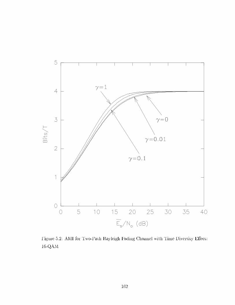
Figure 5.2: AMI for Two-Path Rayleigh Fading Channel with Time Diversity E�ect:
16-QAM
162

= 0:01 = 0:1 = 1
8-PSK 16-QAM 8-PSK 16-QAM 8-PSK 16-QAM
3.5 - 0.2 dB - 1.3 dB - 2.5 dB
3 - 0.1 dB - 0.8 dB - 1.6 dB
AMI 2.5 0.2 dB 0.1 dB 1.1 dB 0.5 dB 2.2 dB 1.2 dB
(Bits/T ) 2 0.1 dB 0.1 dB 0.6 dB 0.3 dB 1.4 dB 0.9 dB
1.5 0 dB 0.1 dB 0.4 dB 0.3 dB 0.9 dB 0.7 dB
1 0 dB 0.1 dB 0.2 dB 0.2 dB 0.6 dB 0.6 dB
Table 5.1: Gain Due to Time Diversity E�ect on the Two-Path Rayleigh Channel
163

5.3.2 Channels with Continuous-Valued Input
The gains which result from the time diversity e�ect are determined here for the case
of a channel with continuous-valued input. All of the assumptions stated for the
discrete-valued input case are assumed to be valid here. In order to determine the
capacity, the AMI will be expressed as a di�erence of entropies in the form
I(X;Y1; Y2j�11;�12;�21;�22; ~X1; ~X2) = H(Y1; Y2j�11;�12;�21;�22; ~X1; ~X2) (5.33)
�H(Y1; Y2jX;�11;�12;�21;�22; ~X1; ~X2):
The entropyH(Y1; Y2jX;�11;�12;�21;�22; ~X1; ~X2) can immediately be determined to
be equal to log(2�e�2N )2. By examining equation (5.22) and (5.23), one can see that
if the variables �11, �12, �21, �22, ~x1, and ~x2 are all known, the only uncertainty is due
to the noise variables n1 and n2. Since these variables are modelled as independent
Gaussian variates, each with entropy log(2�e�2N), the joint entropy is simply equal to
twice this value.
In order to determine the entropy H(Y1; Y2j�11;�12;�21;�22; ~X1; ~X2), certain re-
sults taken from Chapter 3 can be used after some simpli�cation. Once again by
examining the expressions shown in equation (5.22) and (5.23), it is obvious that the
additive terms �12~x1 and �21~x2 have no e�ect on the entropy of Y1 and Y2 conditioned
on knowledge of these variables. The problem may be restated in terms of determin-
ing the entropy H(Y1; Y2j�11;�22), where y1 = �11x + n1 and y2 = �22x + n2. If the
variable X is assumed to have a Gaussian distribution, then equation (3.82) may be
used to write
p(y1; y2j�11; �22) = 1
(2�)2 detBY j�exp
0B@�1
2[y�1 y
�2]B
�1Y j�
264 y1
y2
3751CA (5.34)
where BY j� is the covariance matrix of this joint Gaussian pdf. Since this pdf is
Gaussian, one may immediately write the entropy as
H(Y1; Y2j�11;�22) = Ep(�11)p(�22)nlog
h(2�e)2 detBY j�
io: (5.35)
In this case,
detBY j� = �2Nh�j�11j2 + j�22j2
��2X + �2N
i: (5.36)
164

Since the pdf yielding H(Y1; Y2j�11;�22) is Gaussian, this means that the entropy is
maximized and that the resulting AMI is actually an expression for the capacity of
the channel. This capacity is achieved with a Gaussian distributed input. Using the
information gathered here, the capacity is determined to be
C = Ep(�11)p(�22)
(log
"1 + (j�11j2 + j�22j2)�
2X
�2N
#): (5.37)
This capacity can also be expressed in the form
C = Ep(r)
(log
"1 + r2
�2X�2N
#)(5.38)
where r =qj�11j2 + j�22j2. The variances of the zero mean Gaussian fading variables
�11 and �22 are �2�11= 1
2(1+ )and �2�22
= 2(1+ )
, respectively. If = 1, then the
capacity is the same as that determined for the dual antenna diversity case for the
ideal Rayleigh channel. If 6= 1, then the probability distribution of R is described
by the pdf
p(r) =2(1 + )r
1�
"exp
��(1 + )r2
�� exp
�(1 + )
r2!#
for r � 0: (5.39)
Details of the derivation of this pdf can be found in Appendix E. In order to determine
an explicit expression for the channel capacity, one must evaluate the expression
Z 1
0
2(1 + )r
1�
"exp
��(1 + )r2
�� exp
�(1 + )
r2!#
ln
"1 + r2
�2X�2N
#dr: (5.40)
Making the substitution of variables t = 1+ r2�2X
�2N
allows this integral to be expressed
in the form
�2N (1 + )
�2X(1� )
"exp
(1 + )�2N
�2X
! Z 1
1exp
�(1 + )�2N
�2Xt
!ln tdt (5.41)
� exp�(1+ )�2
N
�2X
� R11 exp
�� (1+ )�2
N
�2X
t�ln tdt
�:
The remaining integrals may be viewed in terms of the exponential integral function.
Doing so results in the capacity being determined as
C =log2 e
1�
24 exp
0@1 +
"�EsN0
#�11AEi0@�1 +
"�EsN0
#�11A (5.42)
� exp�(1 + )
h�EsN0
i�1�Ei
��(1 + )
h�EsN0
i�1��bits=T
165
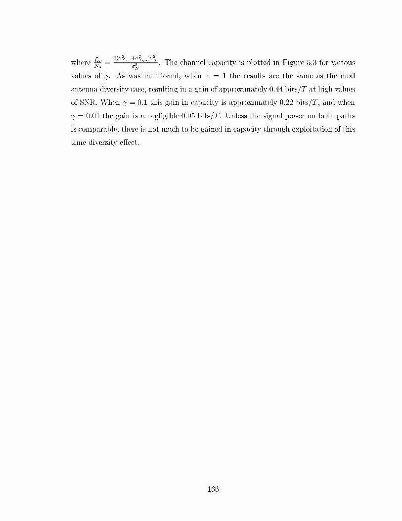
where�EsN0
=2(�2�11
+�2�22)�2X
�2N
. The channel capacity is plotted in Figure 5.3 for various
values of . As was mentioned, when = 1 the results are the same as the dual
antenna diversity case, resulting in a gain of approximately 0.44 bits/T at high values
of SNR. When = 0:1 this gain in capacity is approximately 0.22 bits/T , and when
= 0:01 the gain is a negligible 0.05 bits/T . Unless the signal power on both paths
is comparable, there is not much to be gained in capacity through exploitation of this
time diversity e�ect.
166

Figure 5.3: Capacity of Two-Path Rayleigh Fading Channel with Time Diversity
E�ect
167

Chapter 6
Conclusion
6.1 Summary of Presentation
The practical utility of information theoretic limits as applied to realizable commu-
nication systems is argued in Chapter 1 through an examination of the history of the
telephone line channel. It is pointed out that at one time the information theoretic
capacity of an AWGN channel was considered to be grossly optimistic and extremely
impractical. Today, realistic communication systems approach this theoretic result
to within 3 dB or less. It follows that similar calculations made for multipath fading
channels should also be viewed as reasonably realistic limits. If this is not the case for
any particular situation, then the problem can likely be identi�ed in terms of whether
the channel model used is appropriate. A summary of the state of the art in coding
for fading channels is also given.
Chapter 2 focuses on the fading channel models used in research. A generalized
model is presented �rst, which is based on a physical interpretation of what occurs
when a signal is transmitted over a multipath channel. In order to isolate the e�ects of
amplitude fading, an idealized model is used. Amplitude fading statistics are speci�ed
for a number of di�erent fading situations. The in uence of Doppler spread on various
practical aspects of the channel model is discussed. Time dispersive channels are also
considered, and the modelling of this characteristic is examined. A popular model
for a frequency-selective channel is presented, which due to its simplicity, allows
mathematical analysis to be tractable.
168

The third chapter is intended as a reference for further research dealing with the
design of codes for fading channels. Following a summary of some basic concepts
from the �eld of information theory, limits on the maximum rate of reliable data
transmission are determined for an ideal fading channel. This idealized model is
commonly used in coding research, and the results obtained can be used as an ultimate
benchmark against which to compare code performance. The results are established
in terms of both average and peak transmitted power. Various signal constellations
are considered in order to illustrate the possible trade o� between peak and average
power results. Gains available through the use of space diversity are determined in
terms of information theoretic quantities. The chapter concludes with a statement of
the potential coding gain available on the ideal Rayleigh channel, and a summary of
the best known coding techniques to date.
When the ideal fading channel model is used, it is assumed that the state of the
fading process is known at the receiver. In reality, some scheme must be used to
obtain an estimate of the channel characteristics. Chapter 4 deals with determining
the additional losses in information rate incurred due to the practical limitations of
realistic channel estimation schemes. The necessity of estimating the fading process
is examined �rst, and is accomplished through calculation of limits on the rate of
reliable data transmission when no CSI is available at the receiver. Following this,
information theoretic quantities are determined for a number of practical channel esti-
mation schemes. The particular estimation methods considered are perfect coherent
detection, pilot tone extraction, di�erentially coherent detection, and pilot symbol
transmission. The losses due to non-ideal CSI are determined through comparison
with the results obtained for the ideal channel.
The e�ect of time dispersion on the rate of reliable communication is investigated
in Chapter 5. Application of information theoretic concepts to waveform channels
is discussed �rst. These results are then extended to determine the capacity of a
frequency-selective fading channel speci�ed by the two-path Rayleigh model. A time
diversity e�ect occurs for certain instances of frequency-selective fading. The resulting
gain in the rate of reliable data transmission available through exploitation of this
inherent time diversity is determined for a certain class of waveform channels.
169

6.2 Conclusions
The following list is a synopsis of the principal results adduced in the thesis.
1. When designing coded modulation for an ideal Rayleigh fading channel, a sig-
nal set expansion of 2 is still suÆcient when considering PSK constellations.
For higher levels of QAM, however, an expansion factor of 4 may result in a
signi�cant gain.
2. The capacity of an ideal Rayleigh fading channel with an average power con-
straint is
C = �(log2 e) exp0@" �Es
N0
#�11AEi0@�
"�EsN0
#�11A bits=T: (6.1)
This indicates that the loss in SNR due to Rayleigh fading is no more than 2.51
dB, or equivalently, that the loss in capacity is no more than 0.84 bits/T .
3. For positive integer values of m, the capacity of an ideal Nakagami fading chan-
nel is
C = (log2 e)(�m)m
�(m)
"�EsN0
#�m d
ds
!m�1 �es
sEi (�s)
�bits=T: (6.2)
where s = m�
�EsN0
��1. For positive real values of m, the loss in SNR due to
Nakagami fading is no greater than me� (m), where (�) is Euler's psi function.
4. While PSK is superior with respect to peak power, and QAM is better with
respect to average power, hybrid AMPM constellations show promise in perfor-
mance with respect to both types of constraint.
5. Subject to a peak power constraint, the capacity of an ideal Rayleigh fading
channel is bounded from above by
C � �(log2 e) exp0@" �Ps
N0
#�11AEi0@�
"�PsN0
#�11A bits=T (6.3)
and from below by
C � �(log2 e) exp0@" �Ps
eN0
#�11AEi0@�
"�PseN0
#�11A bits=T: (6.4)
170

The discrepancy between these bounds at high values of SNR is 4.34 dB, or
equivalently, a factor of 1.44 bits/T .
6. The use of space diversity reclaims a signi�cant amount of the loss experienced
due to amplitude fading, even when the fading processes experienced by the
individual antennae are moderately correlated. Most of the gain is achieved by
using 2 or 3 antennae.
7. The capacity of an ideal Rayleigh fading channel with space diversity is the same
as that of an ideal Nakagami fading channel, where the Nakagami parameter
m is set to equal the number of antennae. For example, the capacity of a dual
diversity system is
C = (log2 e)
241 +
0@2
"�EsN0
#�1�11A exp
0@2
"�EsN0
#�11AEi0@�2
"�EsN0
#�11A35 bits=T:
(6.5)
8. The potential coding gain over uncoded QAM in Rayleigh fading increases by
10 dB for each reduction in error probability by a power of 10. For example,
the potential gain is 23.3 dB at a symbol error rate of 10�3, 53.3 dB at an error
rate of 10�6, and 73.3 dB for a symbol error probability of 10�8.
9. When no LOS component exists, the fading process must be estimated in order
to facilitate useable data rates. A Rician channel with R � 10 dB can support
practical data rates without CSI.
10. When the constellation under consideration is large, information transmitted
through the signal amplitude is essentially separable from that transmitted
through the phase. When only the phase of the fading process is determined
at the receiver, the information in the signal amplitude is essentially lost, and
only the information in the signal phase is transmitted reliably. For PSK con-
stellations, phase-only information is adequate.
11. When the phase of the fading process can be determined and the amplitude is
ignored, higher data rates are obtained with a discrete-valued input rather than
with a continuous-valued input.
171

12. Channel estimation by means of pilot tone extraction is essentially ideal for high
values of SNR.
13. Channel estimation by means of di�erentially coherent detection is sensitive to
Doppler spread. This sensitivity increases with larger PSK constellations. The
loss due to Doppler spread can be minimized by considering a constellation
expansion factor of 4 when designing coded modulation.
14. Although pilot symbol detection shows promise for use over channels in which a
LOS component exists, it is extremely sensitive to Doppler spread in Rayleigh
fading environments.
15. Subject to the assumption of being able to track changes in the channel, the
capacity of the two-path Rayleigh channel is the same as that of the ideal at
fading Rayleigh channel.
16. The inherent time diversity due to frequency-selective fading results in an in-
crease of the AMI and capacity of certain waveform channels. This gain can be
as great as that achieved by using dual antenna diversity.
6.3 Suggestions for Further Research
Presented here is a list of issues which merit further consideration.
1. Now that limits on the rate of reliable data transmission over fading channels
have been determined, the next obvious step is to apply these results to the
design of coded modulation for fading channels. Constellation expansion by
a factor of more than 2 shows promise for use in various fading situations.
Investigation of the design and performance of codes based on hybrid AMPM
signal sets for use over non-linear channels may be studied.
2. There is still plenty of work to be done on the modelling of fading channels.
For example, the mobile cellular channel is usually described by a patchwork
of known simple models. For mobile communication in urban areas, a Rayleigh
172

model is often used. However, once a mobile unit moves out of the city envi-
ronment, a Rician model is usually assumed. Changing models in this manner
completely alters the characteristics of the channel. It would be nice if a single
system could be based on a single channel model.
3. Better bounds are needed on information theoretic quantities such as AMI and
entropy. Those based on the notion of entropy power are good for probability
distributions that are close to being Gaussian, but become very weak in other
cases. A good bound for an arbitrary probability distribution is desirable.
4. For the case of non-ideal CSI, bounds on AMI were determined. For certain
input probability distributions, however, it was demonstrated that these bounds
become very weak, and consequently cannot be used as a basis for determining
the capacity of such channels. It is still of interest to determine the capacity of a
channel with non-ideal CSI, as well as the distribution of the capacity achieving
input.
173

Bibliography
[1] C. E. Shannon, \A Mathematical Theory of Communication", Bell Syst. Tech.
J., vol. 27, pp. 379-423 and 623-656, July and Oct. 1948.
[2] R. V. L. Hartley, \Transmission of Information", Bell Syst. Tech. J., vol. 7, pp.
535-563, July 1928.
[3] M.V. Eyubo�glu and G. D. Forney, Jr., \Trellis Precoding: Combined Coding,
Precoding and Shaping for Intersymbol Interference Channels", IEEE Trans.
Inform. Theory, vol. 38, pp. 301-314, March 1992.
[4] G. D. Forney, Jr., R. G. Gallager, G. R. Lang, F. M. Longsta� and S. U. Qureshi,
\EÆcient Modulation for Band-Limited Channels", IEEE J. Select. Areas Com-
mun., vol. SAC-2, pp. 632-647, Sept. 1984.
[5] H. Imai and S. Hirakawa, \A New Multilevel Coding Method Using Error-
Correcting Codes", IEEE Trans. Inform. Theory, vol. IT-23, pp. 371-377, May
1977.
[6] G. Ungerboeck, \Channel Coding with Multilevel/Phase Signals", IEEE Trans.
Inform. Theory, vol. IT-28, pp. 55-67, Jan. 1982.
[7] L. F. Wei, \Rotationally Invariant Convolutional Channel Coding with Ex-
panded Signal Space-Part II: Nonlinear Codes", IEEE J. Select. Areas Com-
mun., vol. SAC-2, pp. 672-686, Sept. 1984.
[8] A. R. Calderbank and N. J. A. Sloane, \New Trellis Codes Based on Lattices
and Cosets", IEEE Trans. Inform. Theory, vol. IT-33, pp. 177-195, March 1987.
174

[9] G. D. Forney, Jr., \Coset Codes-Part I: Introduction and Geometrical Classi�-
cation", IEEE Trans. Inform. Theory, vol. 34, pp. 1123-1151, Sept. 1988.
[10] G. D. Forney, Jr., \Trellis Shaping", IEEE Trans. Inform. Theory, vol. 38, pp.
281-300, March 1992.
[11] G. D. Forney, Jr. and M. V. Eyubo�glu, \Combined Equalization and Coding
Using Precoding", IEEE Communications Magazine, pp. 25-34, Dec. 1991.
[12] C. Berrou, A. Glavieux and P. Thitimajshima, \Near Shannon Limit Error-
Correcting Coding and Decoding: Turbo Codes(1)", Proc. ICC'93 Conf., vol.
2, pp. 1064-1070, Geneva, Switzerland, May 23-26, 1993.
[13] S. Lin and D. J. Costello, Jr., Error Control Coding: Fundamentals and Appli-
cations, Englewood Cli�s, N. J.: Prentice-Hall, 1983.
[14] S. Lin, \A Low-Complexity and High-Performance Concatenated Coding
Scheme for High-Speed Satellite Communications", NASA Tech. Report 93-001,
Feb. 1993.
[15] P. J. McLane, P. H. Wittke, P. K.-M. Ho and C. Loo, \PSK and DPSK Trellis
Codes for Fast Fading, Shadowed Mobile Satellite Communication Channels",
IEEE Trans. Commun., vol. 36, pp. 1242-1246, Nov. 1988.
[16] D. Divsalar and M. K. Simon, \Trellis Coded Modulation for 4800 to 9600 bps
Transmission Over a Fading Satellite Channel", IEEE J. Select. Areas Commun.,
vol. SAC-5, pp. 162-175, Feb. 1987.
[17] D. Divsalar and M. K. Simon, \The Design of Trellis Coded MPSK for Fading
Channels: Performance Criteria", IEEE Trans. Commun., vol. 36, pp. 1004-
1012, Sept. 1988.
[18] L. F. Wei, \Trellis-Coded Modulation with Multidimensional Constellations",
IEEE Trans. Inform. Theory, vol. IT-33, pp. 483-501, July 1987.
[19] D. Divsalar and M. K. Simon, \Multiple Trellis Coded Modulation (MTCM)",
IEEE Trans. Commun., vol. 36, pp. 410-419, April 1988.
175

[20] D. Divsalar and M. K. Simon, \The Design of Trellis Coded MPSK for Fading
Channels: Set Partitioning for Optimum Code Design", IEEE Trans. Commun.,
vol. 36, pp. 1013-1021, Sept. 1988.
[21] E. Zehavi, \8-PSK Trellis Codes for a Rayleigh Channel", IEEE Trans. Com-
mun., vol. 40, pp. 873-884, May 1992.
[22] S. Lin, \Multilevel Coded Modulation for the AWGN and Rayleigh Fading
Channels", Seminar given at Queen's University, May 28, 1993.
[23] S. Le Go�, A. Glavieux and C. Berrou, \Turbo-Codes and High Spectral EÆ-
ciency Modulation", Proc. ICC'94 Conf., vol. 2, pp. 645-649, New Orleans, LA,
May 1-5, 1994.
[24] J. Du and B. Vucetic, \Trellis Coded 16-QAM for Fading Channels", European
Trans. Commun. and Related Tech., vol. 4, pp. 335-341, May-June 1993.
[25] C.-E. W. Sundberg and N. Seshadri, \Coded Modulation for Fading Channels:
An Overview", European Trans. Commun. and Related Tech., vol. 4, pp. 309-
324, May-June 1993.
[26] R. S. Kennedy, Fading Dispersive Communication Channels, New York: Wiley,
1969.
[27] R. G. Gallager, Information Theory and Reliable Communication, New York:
Wiley, 1968.
[28] T. Ericson, \A Gaussian Channel with Slow Fading", IEEE Trans. Inform.
Theory, vol. 16, pp. 353-355, May 1970.
[29] W. C. Y. Lee, \Estimate of Channel Capacity in Rayleigh Fading Environment",
IEEE Trans. Veh. Technol., vol. 39, pp. 187-189, Aug. 1990.
[30] T. Matsumoto and F. Adachi, \Performance Limits of Coded Multilevel DPSK
in Cellular Mobile Radio", IEEE Trans. Veh. Technol., vol. 41, pp. 329-336,
Nov. 1992.
176

[31] K. Leeuwin-Boull�e and J. C. Bel�ore, \The Cuto� Rate of Time Correlated
Fading Channels", IEEE Trans. Inform. Theory, vol. 39, pp. 612-617, March
1993.
[32] L. H. Ozarow, S. Shamai and A. D. Wyner, \Information Theoretic Consid-
erations for Cellular Mobile Radio", IEEE Trans. Veh. Technol., vol. 43, pp.
359-378, May 1994.
[33] J. G. Proakis, Digital Communications, New York: McGraw-Hill, 1983.
[34] W. C. Y. Lee, Mobile Communications Engineering, New York: McGraw-Hill,
1982.
[35] J. K Cavers and P. Ho, \Analysis of the Error Performance of Trellis-Coded
Modulations in Rayleigh Fading Channels", IEEE Trans. Commun., vol. 40,
pp. 74-83, Jan. 1992.
[36] C. Loo, \A Statistical Model for a Land Mobile Satellite Link", IEEE Trans.
Veh. Technol., vol. VT-34, pp. 122-127, Aug. 1985.
[37] A. Papoulis, Probability, Random Variables, and Stochastic Processes, New
York: McGraw-Hill, 1965.
[38] P. J. Crepeau, \Uncoded and Coded Performance of MFSK and DPSK in Nak-
agami Fading Channels", IEEE Trans. Commun., vol. 40, pp. 487-493, March
1992.
[39] M. Nakagami, \The m-Distribution - A General Formula of Intensity Distribu-
tion of Rapid Fading", in Statistical Methods in Radio Wave Propagation, W.
C. Ho�man Ed., New York: Pergamon, 1960.
[40] H. Suzuki, \A Statistical Model for Urban Radio Propagation", IEEE Trans.
Commun., vol. COM-25, pp. 673-680, July 1977.
[41] A. Lee and P. J. McLane, \Convolutionally Interleaved PSK and DPSK Trellis
Codes for Shadowed Fast Fading Mobile Satellite Communication Channels",
IEEE Trans. Veh. Technol., vol. 39, pp. 37-47, Feb. 1990.
177

[42] L. F. Wei, \Coded M-DPSK with Built-In Time Diversity for Fading Channels",
IEEE Trans. Inform. Theory, vol. 39, pp. 1820-1839, Nov. 1993.
[43] W. C. Jakes, Jr., Microwave Mobile Communications, New York: Wiley, 1974.
[44] G. L. Turin, F. D. Clapp, T. L. Johnston, S. B. Fine and D. Lavry, \A Statistical
Model of Urban Multipath Propagation", IEEE Trans. Veh. Technol., vol. VT-
21, pp. 1-9, Feb. 1972.
[45] H. Hashemi, \Simulation of the Urban Radio Propagation Channel", IEEE
Trans. Veh. Technol., vol. VT-28, pp. 213-225, Aug. 1979.
[46] W. D. Rummler, \A New Selective Fading Model: Application to Propagation
Data", Bell Syst. Tech. J., vol. 58, pp. 1037-1071, May 1979.
[47] P. Balaban and J. Salz, \Optimum Diversity Combining and Equalization in
Digital Data Transmission with Applications to Cellular Mobile Radio-Part I:
Theoretical Considerations", IEEE Trans. Commun., vol. 40, pp. 885-894, May
1992.
[48] J. E. Mazo, \Exact Matched Filter Bound for Two-Beam Rayleigh Fading",
IEEE Trans. Commun., vol. 39, pp. 1027-1030, July 1991.
[49] T. M. Cover and J. A. Thomas, Elements of Information Theory, New York:
Wiley, 1991.
[50] A. Papoulis, The Fourier Integral and its Applications, New York: McGraw-Hill,
1962.
[51] G. D. Forney, Jr. and L. F. Wei, \Multidimensional Constellations-Part I: In-
troduction, Figures of Merit, and Generalized Cross Constellations", IEEE J.
Select. Areas Commun., vol. 7, pp. 877-892, Aug. 1989.
[52] A. J. Stam, \Some Inequalities Satis�ed by the Quantities of Information of
Fisher and Shannon", Information and Control, vol. 2, pp. 101-112, June 1959.
[53] N. M. Blachman, \The Convolution Inequality for Entropy Powers", IEEE
Trans. Inform. Theory, vol. IT-11, pp. 267-271, April 1965.
178
[54] I. S. Gradshteyn and I. M. Ryzhik, Table of Integrals, Series, and Products,
Fifth Edition, A. Je�rey Ed., San Diego: Academic Press Inc., 1994.
[55] A. Erd�elyi, W. Magnus, F. Oberhettinger and F. G. Tricomi, Tables of Integral
Transforms, vol. 1, New York: McGraw-Hill, 1954.
[56] L. L. Campbell, Personal Communication, July 19, 1994.
[57] M. K. Simon, \Dual-Pilot Tone Calibration Technique", IEEE Trans. Veh.
Technol., vol. VT-35, pp. 63-70, May 1986.
[58] D. Divsalar and M. K. Simon, \Maximum-Likelihood Di�erential Detection
of Uncoded and Trellis Coded Amplitude-Phase Modulation over AWGN and
Fading Channels - Metrics and Performance", Submitted for publication.
[59] M. L. Moher and J. H. Lodge, \TCMP - A Modulation and Coding Strategy
for Rician Fading Channels", IEEE J. Select. Areas Commun., vol. 7, pp. 1347-
1355, Dec. 1989.
[60] G. T. Irvine and P. J. McLane, \Symbol-Aided Plus Decision-Directed Recep-
tion for PSK/TCM Modulation on Shadowed Mobile Satellite Fading Channels",
IEEE J. Select. Areas Commun., vol. 10, pp. 1289-1299, Oct. 1992.
[61] R. Price, \Nonlinearly Feedback-Equalized PAM vs. Capacity for Noisy Filter
Channels", Proc. ICC'72 Conf., pp. 22.12-22.17, Philadelphia, PA, June 19-21,
1972.
[62] R. Buz, \Design and Performance Analysis of Multi-Dimensional Trellis Coded
Modulation", M.Sc. Thesis, Dept. of Elec. Eng., Queen's University, Kingston,
Ont., Canada, Feb. 1989.
179

Appendix A
Comment on Results Obtained Through
Computer Simulation
Throughout the thesis, it is stated that certain entropy expressions were evaluated
by computer simulation. What this means is that the entropy is presented as a
function of certain random variables, and the statistical expectation of the expression
is evaluated through Monte Carlo averaging. Pseudo-random number generators are
used to obtain the random variables. Expectation is usually taken with respect to
some type of Gaussian distribution. A uniform random variate generator based on the
linear congruential method is used to randomly generate numbers between 0 and 1.
These are then transformed into Gaussian variables by using the polar method. The
expression to be averaged is repeatedly evaluated for di�erent randomly generated
numbers, and the results are added together in an accumulator. The �nal average is
obtained by dividing the contents of the accumulator by the total number of trials.
For the majority of the results obtained, the number of trials performed for a
�xed value of SNR was in the range of 100,000 to 1,000,000. As expressions become
more complex and larger constellations are considered, the duration of a computer
simulation becomes prohibitively long. In some cases, only 20,000 trials were used
due to computer time constraints. Con�dence intervals could be determined by using
a method such as that shown in Appendix A of [62]. However, since the �nal result
for the cases considered is always a number between 0 and 14, the criterion that was
used in judging the quality of the simulation was convergence to at least the second
decimal place of the sample mean.
180

Appendix B
Calculation of Channel Capacity for
Speci�c Fading Distributions
Explicit expressions are derived here for the capacity of ideal Rayleigh and Nakagami
fading channels.
B.1 Capacity of a Rayleigh Fading Channel
The capacity of an ideal fading channel expressed in units of bits/T is given by the
expression
C = Ep(�)
(log2
1 + j�j2�
2X
�2N
!)
= (log2 e)Ep(�)
(ln
1 + j�j2�
2X
�2N
!): (B.1)
For a Rayleigh channel, the fading variable is described by the complex-valued Gaus-
sian pdf
p(�) =1
2��2�exp
� j�j
2
2�2�
!: (B.2)
The expression Ep(�)
�ln�1 + j�j2 �2X
�2N
��can be determined for the Rayleigh case by
evaluating the integral
ZS�
1
2��2�exp
� j�j
2
2�2�
!ln
1 + j�j2�
2X
�2N
!d�: (B.3)
181

By transforming to polar coordinates, where the particular value of the complex
fading variable is represented as � = r cos�+ jr sin�, this integral becomes
1
2��2�
Z 1
0
Z 2�
0r exp
� r2
2�2�
!ln
1 + r2
�2X�2N
!d�dr: (B.4)
After integrating over the phase variable �, the remaining integral is
1
�2�
Z 1
0r exp
� r2
2�2�
!ln
1 + r2
�2X�2N
!dr: (B.5)
Making the substitution t = 1 + r2�2X
�2N
places this integral in the form
�2N2�2��
2X
exp
�2N
2�2��2X
! Z 1
1exp
� �2N2�2��
2X
t
!ln tdt: (B.6)
Using the relation [54, p. 602, 4.331 2.]
Z 1
1e��x lnxdx = � 1
�Ei (��) for <f�g > 0 (B.7)
and the fact that�EsN0
=2�2��
2X
�2N
, the integral in (B.6) can be solved to obtain
Ep(�)
(ln
1 + j�j2�
2X
�2N
!)= � exp
0@" �Es
N0
#�11AEi0@�
"�EsN0
#�11A (B.8)
where Ei(�) is the exponential integral function de�ned by
Ei(x) = �Z 1
�x1
te�tdt for x < 0: (B.9)
Thus, the capacity of an ideal Rayleigh fading channel is given by the expression
C = � (log2 e) exp
0@" �Es
N0
#�11AEi0@�
"�EsN0
#�11A bits=T: (B.10)
B.2 Capacity of a Nakagami Fading Channel
Since Nakagami fading lacks an accompanying phase distribution, it may be assumed
to be uniform over the interval (��; �]. This is usually the case, since small changes
in the channel result in signi�cant variations of the phase. The phase distribution is
not important here anyway, since equation (B.1) only depends upon the magnitude
182

of the fading variable. For the Rayleigh fading case, averaging over the amplitude
distribution is given by equation (B.5). By substituting the Nakagami pdf for the
Rayleigh pdf in equation (B.5), one obtains the integral
2mm
�(m)m
Z 1
0r2m�1 exp
��mr2�ln
1 + r2
�2X�2N
!dr: (B.11)
Making the substitution t =�2X
�2N
r2 changes the form of the integral to
mm
�(m)
�2N�2X
!m Z 1
0tm�1 exp
�m�
2N
�2Xt
!ln(1 + t)dt: (B.12)
A solution for this integral has not been found for arbitrary values of m. However,
if m takes on positive integer values, then an explicit expression for channel capacity
may be obtained. By using the Laplace transform property [55]
Lntm�1f(t)
o= (�1)m�1
d
ds
!m�1F (s) (B.13)
where the functions f(t) and F (s) constitute a Laplace transform pair, and the inte-
gral relation [54, p. 603, 4.337 1.]
Z 1
0e��x ln (� + x) dx =
1
�
hln� � e��Ei (���)
ifor j arg�j < �;<f�g > 0
(B.14)
the capacity of an ideal Nakagami fading channel can be expressed in the form
C = (log2 e)(�m)m
�(m)
"�EsN0
#�m d
ds
!m�1 �es
sEi(�s)
�bits=T: (B.15)
In this equation, the parameter s is de�ned to be equal to m�
�EsN0
��1, where the SNR
relation�EsN0
=�2
X
�2N
is used. For m = 1, this expression yields the capacity of the
Rayleigh channel stated in equation (B.10).
183

Appendix C
Calculation of Asymptotic Loss Due to
Speci�c Fading Distributions
Explicit expressions are derived here for the asymptotic loss in SNR due to ideal
Rayleigh and Nakagami fading.
C.1 Asymptotic Loss Due to Rayleigh Fading
The asymptotic loss due to multipath fading is given by the expression
2�Ep(�)flog2 j�j2g: (C.1)
The base 2 logarithm used in the exponent can be factored to obtain
Ep(�)nlog2 j�j2
o= (log2 e)Ep(�)
nln j�j2
o: (C.2)
Averaging over the Rayleigh fading pdf can be accomplished by evaluating the integral
ZS�
1
2��2�exp
� j�j
2
2�2�
!ln j�j2d�: (C.3)
By transforming to polar coordinates, where � = r cos�+jr sin�, the integral becomes
1
2��2�
Z 1
0
Z 2�
0r exp
� r2
2�2�
!ln r2d�dr: (C.4)
Integrating over the phase variable � leaves
1
�2�
Z 1
0r exp
� r2
2�2�
!ln r2dr: (C.5)
184

Making the substitution t = r2 places the integral in the form
1
2�2�
Z 1
0exp
� t
2�2�
!ln tdt: (C.6)
The solution to this integral is obtained by using the relation [54, p. 602, 4.331 1.]
Z 1
0e��x lnxdx = � 1
�(CE + ln�) for <f�g > 0: (C.7)
The parameter CE is Euler's constant, which is de�ned as
CE = �Z 1
0e�t ln tdt � 0:57721566490 : : : (C.8)
By using the relation given in (C.7), the solution obtained for the expression in (C.6)
is
ln�2�2�
��CE: (C.9)
Since it is assumed that 2�2� = 1 so that the fading has a unity gain, then the desired
solution in this case is
Ep(�)nln j�j2
o= �CE (C.10)
and the asymptotic loss due to fading is
2(log2 e)CE = eCE (C.11)
which is equivalent to 2.51 dB.
C.2 Asymptotic Loss Due to Nakagami Fading
The asymptotic loss due to Nakagami fading can be obtained in the same manner
shown in Appendix C.1 for the Rayleigh channel. By using equation (C.5), and
replacing the Rayleigh pdf with the Nakagami pdf, one obtains
Ep(�)nln j�j2
o=
2mm
�(m)m
Z 1
0r2m�1 exp
��mr2�ln r2dr: (C.12)
After making the substitution t = r2, this expression takes the form
mm
�(m)m
Z 1
0tm�1 exp
��mt�ln tdt: (C.13)
185

The relation [54, p. 604, 4.352 1.]
Z 1
0x��1e��x lnxdx =
1
���(�) [ (�)� ln�] for <f�g > 0;<f�g > 0 (C.14)
can be used to evaluate the integral in equation (C.13). Assuming = 1 so that the
fading gain is set to unity, the solution is
Ep(�)nln j�j2
o= (m)� ln(m) (C.15)
where (�) is Euler's psi function, and is de�ned by the expression
(x) =d
dxln �(x): (C.16)
The function �(�) is known as the gamma function or generalized factorial. The
asymptotic loss due to Nakagami fading is
2log2 e[ln(m)� (m)] = me� (m): (C.17)
For the case m = 1, (1) = �CE, which gives the proper value for the Rayleigh
channel. It is important to note that equation (C.17) is not restricted to integer
values of m, but is valid for any m > 0.
186

Appendix D
Calculation of Error Probability for
Uncoded Modulation in Ideal Rayleigh
Fading
Expressions are derived here for the performance of uncoded modulation used over
an ideal Rayleigh fading channel. An approximation to the symbol error probability
is obtained for QAM constellations. An expression for the bit error probability of
uncoded QPSK is also determined.
D.1 Symbol Error Probability for Uncoded QAM
Suppose that the received channel symbol takes the form Y = �X +N , where X is
a point from a QAM constellation, � is a complex-valued Gaussian fading variable,
and N is a sample of a complex-valued zero mean AWGN process. If a particular
symbol X = xi is an interior point of the constellation where the minimum separation
between QAM symbols is a distance d, then the usual decision region for this point
will be a square of side length d centered on xi. When � = �, the e�ect of the
fading variable in the product �X is a scaling of the coordinates of xi by a factor
r = j�j, as well as a rotation of the point through an angle � = arg � about the origin.
If � is known to equal � at the receiver, then the e�ect of the phase rotation can
be compensated for. After adjusting the phase, the decision region for the symbol
X = xi is chosen as a square of side rd centered on rxi. Given the knowledge that
187
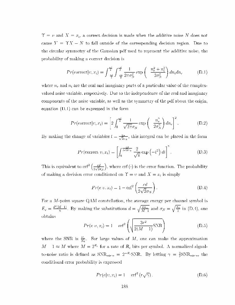
� = � and X = xi, a correct decision is made when the additive noise N does not
cause Y = �X + N to fall outside of the corresponding decision region. Due to
the circular symmetry of the Gaussian pdf used to represent the additive noise, the
probability of making a correct decision is
Pr(correctj�; xi) =Z rd
2
� rd2
Z rd2
� rd2
1
2��2Nexp
�n
2r + n2i2�2N
!dnidnr (D.1)
where nr and ni are the real and imaginary parts of a particular value of the complex-
valued noise variable, respectively. Due to the independence of the real and imaginary
components of the noise variable, as well as the symmetry of the pdf about the origin,
equation (D.1) can be expressed in the form
Pr(correctj�; xi) ="2Z rd
2
0
1p2��N
exp
� n2r2�2N
!dnr
#2: (D.2)
By making the change of variables t = nrp2�N
, this integral can be placed in the form
Pr(correctj�; xi) ="Z rd
2p2�N
0
2p�exp
��t2
�dt
#2: (D.3)
This is equivalent to erf2�
rd2p2�N
�, where erf (�) is the error function. The probability
of making a decision error conditioned on � = � and X = xi is simply
Pr(ej�; xi) = 1� erf2
rd
2p2�N
!: (D.4)
For a M -point square QAM constellation, the average energy per channel symbol is
Es =d2(M�1)
6. By making the substitutions d =
q6EsM�1 and �N =
qN0
2in (D.4), one
obtains
Pr(ej�; xi) = 1� erf2
0@vuut 3r2
2(M � 1)SNR
1A (D.5)
where the SNR is EsN0. For large values of M , one can make the approximation
M � 1 � M where M = 2Rc for a rate of Rc bits per symbol. A normalized signal-
to-noise ratio is de�ned as SNRnorm = 2�RcSNR. By letting = 32SNRnorm, the
conditional error probability is expressed
Pr(ej�; xi) = 1� erf2 (rp ) : (D.6)
188

Assuming the constellation points to be equiprobable, averaging over the pmf p(xi)
results in Pr(ej�) = Pr(ej�; xi). In order to remove the dependence upon �, equation
(D.6) must be averaged over the pdf p(�). Assuming a Rayleigh fading channel, this
is accomplished by evaluating the expression
Pr(e) = 1�Z 1
0
r
�2�exp
� r2
2�2�
!erf2 (r
p ) dr: (D.7)
The complementary error function is de�ned as erfc(�) = 1 � erf(�). This relation,
along with the change of variables s = rp , can be used to write equation (D.7) in
the form
Pr(e) = 1� 1
�2�
"Z 1
0s exp
� s2
2�2�
!ds�
Z 1
02s exp
� s2
2�2�
!erfc(s)ds (D.8)
+Z 1
0s exp
� s2
2�2�
!erfc2(s)ds
#:
Making the change of variables u = s2 for the �rst integral in this expression allows
it to be evaluated as
Z 1
0s exp
� s2
2�2�
!ds =
1
2
Z 1
0exp
� u
2�2�
!du = �2� : (D.9)
By using the integral relation [54, p. 678, 6.287 2.], the second integral is evaluated
to be
Z 1
02s exp
� s2
2�2�
!erfc(s)ds = 2�2�
241� 1q
(2�2� )�1 + 1
35 : (D.10)
The integral relation in [54, p. 941, 8.258 2.] can be used to solve the �nal integral
in the form
Z 1
0s exp
� s2
2�2�
!erfc2(s)ds = �2�
2641� 4
�
arctan�q
1 + (2�2� )�1�
q1 + (2�2� )
�1
375 : (D.11)
After substituting the solved integrals back into equation (D.8), the probability of
detection error is determined to be
Pr(e) = 1� 2p1 + � �1
�1� 2
�arctan
�q1 + � �1
��(D.12)
where � = 2�2� . In terms of the normalized SNR, � = 32SNRnorm where the average
received normalized signal-to-noise ratio isSNRnorm = 2�2�SNRnorm.
189

Due to the edge e�ects of the constellation, this is actually an upper bound on
symbol error probability. However, as the constellation gets larger, this expression
becomes increasingly accurate.
D.2 Bit Error Probability for Uncoded QPSK
Assume that X = xi is a QPSK symbol with coordinates (d; d). The decision region
for this symbol is the �rst quadrant of the Cartesian coordinate system in which it is
represented. The e�ect of a given value of the fading variable � = � is to scale the
coordinates by a factor r and rotate the point through an angle � about the origin. If
the fading variable � is known to equal � at the receiver, then the phase rotation can
be compensated for and the decision regions for all QPSK symbols remain the same.
The only di�erence is that the received symbol will be viewed as having coordinates
(rd; rd). Assuming a Gray mapping of the data bits, a single bit error occurs if the
received symbol falls into an adjacent quadrant, and two bit errors occur when the
received symbol falls into the diagonally opposite quadrant. In terms of the pdf p(n)
of the additive noise variable, this can be expressed as
Pr(bit errorj�; xi) =Z �rd
�1
Z 1
�rdp(n)dn+
Z 1
�rd
Z �rd
�1p(n)dn+ 2
Z �rd
�1
Z �rd
�1p(n)dn:
(D.13)
This can be simpli�ed into the form
Pr(bit errorj�; xi) = 2Z �rd
�1
Z 1
�11
2��2Nexp
�n
2r + n2i2�2N
!dnidnr (D.14)
where nr and ni are the real and imaginary parts of a particular value of the complex-
valued noise variable, respectively. The variable ni vanishes after integrating over the
interval (�1;1), and the remaining integral may be expressed in the form
Pr(bit errorj�; xi) = 1� erf
r
sd2
2�2N
!(D.15)
where erf (�) is the error function. The energy per data bit is Eb = d2 and the noise
power is N0 = 2�2N , so equation (D.15) may also be written in the form
Pr(bit errorj�; xi) = 1� erf
r
sEbN0
!: (D.16)
190

Assuming the QPSK symbols occur with equal probability, the symmetry of the
constellation and the Gray mapping ensure that Pr(bit errorj�) = Pr(bit errorj�; xi).For a Rayleigh fading channel, averaging over the fading variable � requires evaluation
of the expression
Pr(bit error) =Z 1
0
r
�2�exp
� r2
2�2�
!"1� erf
r
sEbN0
!#dr: (D.17)
Using the integral relation in [54, p. 678, 6.287 2.], equation (D.17) is evaluated to
be
Pr(bit error) = 1� 1r1�
��EbN0
��1 (D.18)
where�EbN0
=2�2�EbN0
. This expression yields the probability of bit error per QPSK
symbol. In order to represent the average probability of a data bit being in error,
equation (D.18) must be divided by the number of bits per symbol. After performing
this �nal step, the average bit error probability is determined to be
Pb =1
2
26641� 1r
1��
�EbN0
��13775 : (D.19)
191

Appendix E
Derivation of a PDF Related to the
Two-Path Rayleigh Channel
When considering the two-path Rayleigh channel with Nyquist pulse signalling, a
given transmitted symbol X = x will a�ect only two of the received channel sym-
bols when the delay between the two propagation paths is an integer multiple of the
signalling interval T . In one of these output symbols it appears as an additive term
�1x and in the second it appears in the form �2x, where �1 and �2 are independent
complex-valued Gaussian variables with zero mean. The sum of the squared magni-
tudes of these terms is (j�1j2 + j�2j2)jxj2, and it is of interest to �nd the pdf p(r) of
the random variable R, where R is de�ned by the expression
R =qj�1j2 + j�2j2: (E.1)
By de�ning R1 = j�1j and R2 = j�2j to be the magnitudes of the complex-valued
variables, one may state equation (E.1) in the form
R2 = R21 +R2
2 (E.2)
where
p(r1) =r1�2�1
exp
� r212�2�1
!for r1 � 0 (E.3)
and
p(r2) =r2�2�2
exp
� r222�2�2
!for r2 � 0: (E.4)
192

De�ne two new random variables Z1 and Z2 to be equal to R21 and R
22, respectively. By
performing the required transformation of variables, the probability density functions
given in equations (E.3) and (E.4) can be used to obtain
p(z1) =1
2�2�1
exp
� z12�2�1
!for z1 � 0 (E.5)
and
p(z2) =1
2�2�2
exp
� z22�2�2
!for z2 � 0: (E.6)
Let the random variable Y be de�ned to equal the sum Z1 + Z2. Given knowledge
that the value of Z1 is z1, the conditional pdf
p(yjz1) = 1
2�2�2
exp
�s� z1
2�2�2
!for y � z1 (E.7)
results from equation (E.6) by performing a translation of the variable z2. Through
evaluation of the expressionR y0 p(yjz1)p(z1)dz1, the pdf p(y) is obtained. Assuming
that �2�16= �2�2
, this is easily calculated to be
p(y) =1
2(�2�1� �2�2
)
"exp
� y
2�2�1
!� exp
� y
2�2�2
!#for y � 0: (E.8)
The desired pdf is for the random variable R, which is equal topY . By performing
the appropriate change of variables, one obtains
p(r) =r
(�2�1� �2�2
)
"exp
� r2
2�2�1
!� exp
� r2
2�2�2
!#for r � 0: (E.9)
In order to ensure that E fR2g = 1, the variances of the originating Gaussian dis-
tributions are set to �2�1= 1
2(1+ )and �2�2
= 2(1+ )
, where is the power ratio�2�2�2�1
.
Using this in equation (E.9) places the pdf in the form
p(r) =2(1 + )r
1�
"exp
��(1 + )r2
�� exp
�(1 + )
r2!#
for r � 0: (E.10)
When = 1, this pdf is indeterminate. However, by applying L'Hopital's rule,
one obtains the pdf of a chi distribution with four degrees of freedom. This is the
expected result which would have been obtained if it was assumed that �2�1= �2�2
at
the beginning of the derivation of p(r).
193

Vita
Personal Information
Name: Richard Buz
Date of birth: January 10, 1962
Birth place: Sudbury, Ontario, Canada
Education
1994 Ph.D. in Electrical Engineering (Present Program)
Queen's University, Kingston, Ontario, Canada
1989 M.Sc. in Electrical Engineering
Queen's University, Kingston, Ontario, Canada
1987 B.Sc.(Hons.) in Mathematics and Engineering
Queen's University, Kingston, Ontario, Canada
Awards
1987-88 Queen's Graduate Fellowship, Queen's University
1987 Paithouski Prize, Queen's University
194

Work Experience
1989-94 Computer System Manager
Telecommunications Research Institute of Ontario
1987-89 Teaching Assistant
Department of Electrical Engineering, Queen's University
Publications
� R. Buz, \Uniformity of Non-linear Trellis Codes", in Coded Modulation and
Bandwidth-EÆcient Transmission, edited by E. Biglieri and M. Luise, Amster-
dam: Elsevier, 1992.
� R. Buz, \Signal Mapping and Nonlinear Encoder for Uniform Trellis Codes",
Proc. Globecom'90 Conf., pp. 907.1.1-907.1.7, San Diego, CA, Dec. 2-5, 1990.
� L. Berg, R. Buz, P. J. McLane and M. Turgeon, \Design Procedure for Optimum
or Rotationally Invariant Trellis Codes", Proc. ICC'90 Conf., pp. 607-613,
Atlanta, GA, April 16-19, 1990.
� R. Buz and P. J. McLane, \Error Bounds for Multi-Dimensional TCM", Proc.
ICC'89 Conf., pp. 1360-1366, Boston, MA, June 11-14, 1989.
195


