Interferograms measured by a Fourier transformspectrometer (FTS) usually yield complex spectra be-cause of phase errors, which are due to the measure-ment setup. The phase of these complex spectraneeds to be corrected to separate the different radia-tion sources and to retrieve the scene spectrum. Inabsorption spectrometry, where the radiation fromthe scene is much stronger than the self-emission ofthe instrument, the phase error attributable to themeasurement simply equals the total phase of themeasured spectrum and can easily be corrected.1,2 Inemission spectrometry, however, the self-emission ofthe instrument may contribute significantly to thetotal measurement signal. In this case, the variousradiation contributions and their phase relations
have to be taken into account to separate the differ-ent sources. The self-emission of the beam splitter inthe interferometer, which shows a phase of approx.��2 relative to the scene, particularly needs to beconsidered. If the phase is not properly corrected, theradiometric accuracy of the calibrated spectra is se-riously degraded. Various phase correction methodsfor emission spectrometry have been proposed.3–5
These methods, however, are not applicable for theballoonborne Michelson Interferometer for PassiveAtmospheric Sounding (MIPAS-B2), therefore a newphase determination and correction method has beendeveloped. Section 2 gives an overview of the instru-ment. In Section 3 the interferometer is describedwith its different radiation sources and phase rela-tions. The resulting phase and the problem of phasecorrection is discussed in Section 4. The developedphase correction algorithm is then described in Sec-tions 5 and 6. Finally, an error analysis for this phasecorrection method is presented in Section 7.
2. Instrument Description
The balloonborne MIPAS-B2 is a cryogenic FTS,which is designed to measure concentration profilesof various trace gases in the stratosphere and uppertroposphere (see, e.g., Wetzel et al.,6 Stowasser et al.,7and the references cited therein) and is also used forvalidation of satellite measurements.8,9 The instru-ment measures the atmospheric self-emission in the
A. Kleinert ([email protected]) is with the Institut fürMeteorologie und Klimaforschung, Forschungszentrum Karlsruhe,Postfach 3640, 76021 Karlsruhe, Germany. When this work wasperformed O. Trieschmann ([email protected]) was also with theInstitut für Meteorologie und Klimaforschung. He is now with theEuropean Maritime Safety Agency, Av. Dom João II, Lote 1.06.2 5,1990 Lisbon, Portugal.
Received 30 May 2006; revised 15 December 2006; accepted 19December 2006; posted 19 December 2006 (Doc. ID 71535); pub-lished 3 April 2007.
thermal infrared (IR) spectral region (approximately4–14 �m) from a stratospheric balloon using the limbsounding technique with tangent altitudes up to40 km. A detailed description of the instrument isgiven by Friedl-Vallon et al.10 The optics of MIPAS-B2is made up of a telescope, a double-pendulum inter-ferometer, and a detector system that is housed in aliquid helium cooled cryostat. The optical path differ-ence is measured by a He–Ne reference laser, whichpasses through the interferometer parallel to the IRbeam. The maximum optical path difference ofMIPAS-B2 is �14.5 cm, corresponding to a spectralresolution of 0.0345 cm�1 (unapodized). To achieve ahigh detection sensitivity, the instrument is cooled toapproximately 215–220 K, which reduces its self-emission to the level of the radiation measured fromthe scene. The typical radiation power on the detec-tors is in the range of 10�9–10�6 W. In this experi-mental setup, the various sources that contribute tothe measured signal are of the same order of magni-tude. The total phase of the complex spectrum is thusdependent on the amplitudes of the individual radi-ation contributions. These different contributionshave to be taken into account for the phase correctionof the spectra in order not to deteriorate the radio-metric accuracy.
3. Interferometer
The principle of a Michelson interferometer is dis-played in Fig. 1. An incident collimated beam withthe intensity spectrum S��� (� � 1�� : wavenumber)is split up into two partial beams by the beam splitterBS. The partial beams are reflected back at the mir-rors (retroreflectors) R1 and R2 and are recombined atthe beam splitter. By varying the position of the mov-able retroreflector R2, an optical path difference (x)between the two partial beams of the interferometeris generated.11 Depending on the optical path differ-ence and the wavenumber of the incident radiation,constructive and destructive interferences occur inthe recombined beam, which is focused onto the IR
detector. The signal of the detector is called the in-terferogram IFG(x).
The beam-splitter unit consists of the beam-splitting layer itself, which is mounted on a sub-strate, and a compensation plate, which is made ofthe same material as the beam-splitter substrate tomaintain the symmetry of optical elements betweenboth optical arms.
The radiation, which is modulated by the inter-ferometer, originates from different sources. Thesesources are12:
1. The scene radiation emitted from atmosphericmatter together with the emission from the opticalcomponents of the instrument that are located be-tween the entrance door and the beam splitter (tele-scope and folding mirrors),
2. The emission of the optical components be-tween the beam splitter and the detector (the foldingmirrors and the window of the detector cryostat),which passes through the interferometer in the op-posite direction, and
3. The thermal radiation, that is emitted by thebeam splitter itself.
The radiation of source (1) exhibits the same numberof transmissions and reflections at the beam splitterwithin the optical path of both interferometer arms.Therefore this radiation will be referred to as thebalanced beam. For radiation source (2), the numberof reflections and transmissions is not the same in thetwo optical arms of the interferometer, leading to aso-called unbalanced beam. Beam splitter (3) is emit-ting differently into the two arms, and the number ofreflections and transmissions is different as well. Itcannot be described by one of the aforementionedbeams and is treated separately. A detailed analysisof the spectra generated by the three different portshas been performed by Thériault,13 Trieschmann andWeddigen,14 and Hase et al.15 In this section, thecontributions of the different beams to the IFG areprovided as a basis for later understanding of thephase problem of Fourier spectrometers.
Let S be the intensity of the incident radiation.This radiation is partly modulated in the interferom-eter, and the resulting IFG is composed of a constantradiation contribution and a contribution that varieswith the wave number � and the optical path differ-ence x. For the three radiation contributions we ob-tain:
The indices b, u, and bs stand for balanced beam,unbalanced beam, and beam-splitter emission, re-Fig. 1. Schematic of a FTS with the various radiation sources.
spectively. The indices 1 and 2 denote the amplitudesof the unmodulated and the modulated radiation.The IFG of the unbalanced beam shows a phase shiftof � with respect to the balanced beam; the beamsplitter emission is shifted by ��2. The additionalphase angles u and bs in the equations for the un-balanced beam and the beam-splitter emission, re-spectively, are attributable to the absorption of thebeam splitter.15,16 The magnitude of these phase an-gles has been estimated for the MIPAS-FT instru-ment by Hase et al.15 to be of the order of 10 to 50mrad. MIPAS-B2 uses the same type of beam split-ters with the same emissivity (typically between 0.05and 0.1 at its maximum), therefore this result can beassigned to MIPAS-B2 as well. Since these angles areclose to zero, they will be neglected in the following.The effect of neglecting these angles on the phaseaccuracy will be discussed in Subsection 7.D.
The total IFG is obtained from the sum of the par-tial IFGs, IFGb,u,bs, of the different sources. Further-more it is integrated over all wavenumbers. Theintegral can be written in a more convenient wayusing the following postulations: Sb,u���� � Sb,u���,and Sbs���� � �Sbs���. The unmodulated term of theIFG is eliminated instrumentally by means of high-pass filtering and will not be mentioned any further.Likewise, the index 2 is omitted. The IFG is thensummarized in a single equation
IFG�x� ����
�
�Sb��� � Su��� iSbs����ei2��xd�, (2)
which is equivalent to a complex Fourier transform.Vice versa, the spectrum is obtained as the Fourierbacktransform of the IFG(x):
S��� � FT��IFG�x�� � Sb��� � Su��� iSbs���. (3)
In the complex plane, the balanced radiation is realand positive, the unbalanced radiation is real andnegative, and the beam-splitter emission is purelyimaginary. The natural phase angle �n is determinedby the amplitudes of the three contributions:
tan��n� �Sbs
Sb � Su. (4)
With the cooled setup of the MIPAS-B2 interferom-eter, the radiation intensities �Sb � Su� and Sbs are ofthe same order of magnitude, especially in the longwavelength spectral range and for atmospheric mea-surements at high tangent altitudes of the limbsounding.
Figure 2 shows the real part �Sb � Su� and theimaginary part Sbs of a measured spectrum with ablackbody and deep space as source. (For the deep-space measurements, the instrument is looking 20°upward from the balloon altitude of 30 to 40 km.) The
imaginary part, which represents the beam-splitteremission, is the same for both spectra. The base lineof the deep-space spectrum is mainly determined bythe mirrors of the instrument and the window (ZnSe)of the detector cryostat. Below 820 cm�1, unbalancedradiation predominates, which is expressed by thenegative base line.
The intensity of the beam-splitter signal is onlyapproximately 10% of the blackbody signal, but it isof the same order of magnitude as the real part of thedeep-space spectrum. The intensity of the atmo-spheric spectra is typically between the blackbodyand the deep-space spectra shown here.
4. The Phase Components of a Spectrum
The symmetries given in the previous section, how-ever, are not necessarily valid in measured, sampledIFGs. In the measured IFG, a specific sampling pointis assumed as the point of zero optical path difference(ZOPD) between the two interferometer arms. Thispoint, however, is usually not identical with the realposition of the ZOPD in the continuous IFG. Further-more the real ZOPD is wavenumber dependent. Theshift between the assigned and the real ZOPD is de-fined as and changes with the wavenumber. Thisshift is caused by various reasons, which cannot beavoided in the experimental setup:
Y The position of the movable mirror is deter-mined with a reference laser, which passes the inter-ferometer in parallel to the IR beam. The time delayof the analog amplifiers of the IR signal varies withfrequency (and therefore with wavenumber) and isdifferent from the delay of the laser reference signal.This leads to a wavenumber dependent difference inthe optical path between the IR IFG and the refer-ence signal.
Y The beam splitter is built up of various dielec-tric layers. Thus the mean positions of the effectivebeam-splitting boundary layer vary with the wave-
Fig. 2. Real and imaginary parts of a phase corrected spectrumwith a blackbody and a deep space (looking 20° upward) as source.The imaginary part, which represents the beam-splitter emission,is the same in both cases.
number leading to a wavenumber-dependent ZOPDposition.
Y Dispersion of the substrate material of thebeam splitter and the compensation plate also leadsto optical path differences between both arms thatvary as a function of the wavenumber, if the thick-ness of both substrates is not perfectly identical. Asthe substrates are wedged, a slightly varying thick-ness has to be expected owing to the manufacturingprocess.
Y Another asymmetry occurs because of the dis-crete sampling of the IFG, since the location of theIFG point, which is considered to be the ZOPD, doesnot coincide with the real physical IFG origin atx � 0 (sampling error).
The first three effects cause a wavenumber-dependent position error 1 � 1���. They are depen-dent on the instrument, but rather constant withtime, as the optical and electric components are in-fluenced only by temperature fluctuations. The lasteffect causes a position error of 2 � const, which isthe same for all wavenumbers, but may vary frommeasurement to measurement.
The asymmetric, measured interferogram IFGm�x�is expressed mathematically by the distance fromthe real path-length difference x to the measuredpath difference x , where � 1��� 2. Hence themeasured spectra are expressed as
Sm��� ����
�
IFG �x 1��� 2�e�i2��xdx,
�ei 2�� 1���Ç
inst���
ei 2�� 2Ç
lin���
S���. (5)
The measured spectrum Sm��� is rotated in thecomplex plane by a measurement phase angle m���� inst��� lin��� with respect to the undisturbedspectrum S���. The phase of the first exponentialfunction on the right side of Eq. (5) is caused by theinstrument and is named the instrumental phaseinst��� � 2�� 1���. The second term is due only tothe sampling and increases linearly with the wave-number. It is referred to as the linear phase lin
� 2�� 2.
m��� � inst��� lin��� � 2��� 1��� 2�. (6)
The total phase tot���, which is directly obtainedfrom the phase angle of the complex spectral vectorSm��� now consists of the natural phase angle �n [seeEq. (4)] together with m. In Fig. 3, the spectral con-tributions with their phase angles in the complexplane are summarized in a vector diagram for a spe-cific wavenumber �0. Since the natural phase �n cor-relates with the line structure in the spectrum, thisphase effect is neither comparable with the instru-mental phase nor with the linear phase.
5. Phase Correction
In the true spectrum S���, the balanced port, whichcontains the desired atmospheric radiation, is realand positive. To obtain this spectrum, a phase cor-rection of the measured spectrum must be performedwhere the spectrum is rotated back in the complexplane by the measurement phase m���:
S��� � e�im���Sm���. (7)
A. Phase Correction Methods
In absorption spectrometry, where the radiation fromthe source is much stronger than the self-emission ofthe instrument and the beam splitter, the naturalphase angle �n is very close to zero, and the measure-ment phase m is equal to the total phase �tot, whichis then simply the phase of the spectral vector Sm���in the complex plane.1 Forman et al.2 introduced acorrection in the IFG domain. There, the Fourier-transformed phase function is convolved with the in-terferogram.
In the case of significant beam-splitter emission, itis of crucial importance to neatly separate the mea-surement phase m from the natural phase angle �n.Several methods that consider beam-splitter emis-sion are in use to determine the measurement phaseor perform the phase correction:
Y Revercomb et al.3 determined the self-emissionof the instrument by looking into a cold blackbody.This instrumental contribution, including the beam-splitter emission, is subtracted from each measure-ment before a phase correction is applied. However,for this very general and elegant method it is man-datory that the measurement phase m remain con-stant between two calibration measurements. Onlychanges in the sampling error 2 by an integer num-ber of sampling points can be eliminated. Continuouschanges of the measurement phase, e.g., because ofthermal warping of the interferometer, would lead toradiometric errors in the calibrated spectra.
Y The differential method proposed by Weddigenet al.12 and Blom et al.4 has been developed for theaircraft instrument MIPAS-FT. The method is based
Fig. 3. Phase relations for a specific wave number �0. The radi-ation contributions Sb, Su, and Sbs define the natural phase angle�n. Due to the measurement phase m, the balanced and unbal-anced radiation are rotated from the real axis into the complexplane.
on the amplitude of the difference of adjacent spec-tral points and can be applied only if the gradientsat the line wings are sufficiently strong, such thatthe difference vector dominates over the noise con-tribution. The balloonborne measurements do notalways provide sufficiently strong lines to allow aphase determination using this method with a sat-isfying accuracy.
Y A method developed by Johnson et al.5 is fo-cused on mostly one-sided IFGs. In the case of mostlyone-sided IFGs, phase errors lead to an asymmetry inthe spectral lines. This feature is used to correct forphase errors. A statistical criterion is applied to de-termine the phase that provides the best line shape.This method has the same problem as the above-mentioned differential method, in that the phase cor-rection becomes rather inaccurate in the case of weaklines with a poor signal-to-noise ratio.
These methods are not suited for the phase correc-tion of the spectra measured with MIPAS-B2. Themeasurement phase m of our spectra is not alwayssufficiently stable to allow the use of the method pre-sented by Revercomb et al. The other methods do notprovide satisfactory results in the case of low atmo-spheric radiances as they are measured from a bal-loon altitude of 30 to 40 km. Therefore a new phasecorrection method has been developed, which issuited for two-sided IFGs of atmospheric emissionspectra with low radiation intensities. The method iscapable of:
Y Correcting for continuous changes in the linearphase. (Only nonlinear phase contributions need tobe stable between two calibration sequences.)
Y Calculating the accuracy of the phase correc-tion for each individual IFG, providing a tool for thequality check of the data.
Y Phase correcting spectra with a weak signaland low signal-to-noise ratio.
The phase correction is separated into two steps: Ina first step, the instrumental phase is determinedfrom blackbody measurements (Subsection 5.B), there-after the linear phase is determined individually foreach IFG (Subsection 5.C and Section 6).
B. Instrumental Phase
The instrumental phase, which is governed by theinstrument properties and varies only slowly in time(see Section 4), is derived from blackbody measure-ments SBB���. The beam-splitter emission contributesusually with less than 10% to the blackbody spec-trum. Therefore the natural phase angle �n of theblackbody measurements is very small, and the as-sumption of m � �tot is justified. (A correction of theerror made by this assumption is described in Sub-section 6.B.) The measurement phase is calculatedusing
m��� � �tot,BB��� � arctan 2�Sm,BB����. (8)
The arctan 2 function represents an arctangent func-tion over all four quadrants with a value range from�� to �.
As the blackbody spectrum is a smooth functionwithout high-resolution features, the phase may beobtained from the low-resolution complex spectrum(resolution � 0.5 cm�1). Because of the low resolution,the noise is decreased substantially.
The measurement phase calculated from Eq. (8)comprises the instrumental phase as well as the lin-ear phase of the blackbody measurement. A straightline is fitted and subtracted from the phase m toobtain the instrumental phase inst, which then con-tains only the nonlinear contribution of the phase.Usually the instrumental phase barely varies fromone blackbody measurement to the next one (typi-cally a time interval of 30 to 60 min) and can beassumed constant for the time inbetween. Residualphase variations are considered within the error es-timation (Section 7). It should be emphasized that thesubtraction of the straight line not only comprises thesampling error but also any part of the instrumentalphase that is linear within the spectral channel (e.g.,a linear contribution owing to dispersion in the beamsplitter). Therefore this straight line does not neces-sarily pass through the origin. The instrumentalphase shall in the following be understood as thenonlinear part of the measurement phase.
C. Linear Phase
The linear phase is mainly attributable to the offsetbetween the digitized ZOPD and the real ZOPD, butalso a (thermally induced) misalignment of the inter-ferometer can introduce a linear phase. This phasecan change abruptly from one IFG to another, e.g.,after a reset of the electronics when the ZOPD isnewly defined. Thermal effects can induce a contin-uous variation of the linear phase on a time scale ofseveral minutes. For these reasons, the linear phasehas to be determined on a shorter time scale thanthe instrumental phase. If the phase is sufficientlystable (i.e., the changes are below �100 mrad), IFGsof the same scene (tangent altitude of the limb scan)and sweep direction may be coadded, and only onesingle linear phase has to be determined for the co-added IFG. Otherwise the linear phase has to bedetermined for each interferogram individually. Thephase stability can easily be controlled by calculatingthe total phase �tot because the natural phase �n isconstant for a constant target in the atmosphere.
The linear phase as a function of the wavenumber� can be parameterized by a slope a1 and a point a0� lin��0�. For �0 a wavenumber value in the middleof the spectral range is chosen to keep the error prop-agation effects small. The phase function attributableto the measurement is then written as
m��� � inst��� a0 a1�� � �0�, (9)
where inst��� is determined as described in Subsec-tion 5.B.
The parameters a0 and a1, which define the linearphase, are determined by the use of a statisticalmethod, which is described in the following.
6. Statistical Approach for Phase Correction
The idea underlying phase determination as a statis-tical variable is that no atmospheric lines may berecognizable in the imaginary part of the spectrum,which should contain only the continuous beam-splitter emission [see Eq. (3)] and noise, which isstatistically distributed. Thus the lines must bemapped completely in the real part of the spectrum.The phase is iteratively adjusted using statisticalquantities as correlation and variance in order tomeet this mapping criterion. Therefore this method iscalled a statistical approach. The assumption made isentirely true only if there is no gas in the instrument,which can cause absorption lines in the beam-spitterspectrum and emission lines in the unbalanced beam.This problem will be discussed in Subsection 7.D. Theassumption that no atmospheric lines may be recog-nizable in the imaginary part of the spectrum leads tothe following statements:
1. The correlation � between the real part and theimaginary part of the corrected spectrum S��� is sup-posed to disappear. The slowly varying filter func-tions of the optical and electric components affect allradiation contributions in the same way, thereforethese components of the spectrum are removed byhigh-pass filtering (HP). With a spectral resolution of0.0345 cm�1, a limit of 0.069 cm�1 for the high-passfilter has been proven to be reasonable. The correla-tion of the high-pass filtered spectrum is given as
��Re�SHP�, Im�SHP�� � i
�Re�SHP��i��· Im�SHP��i��� → � 0, (10)
where i is the index of the discrete sampling points.2. The imaginary part of the spectrum should not
contain any line features but only the broadbandbeam-splitter emission together with noise. Thismeans that the variance v over all points of the imag-inary part of the high-pass filtered spectrum shouldreach a minimum. This is achieved by setting the firstderivative of the variance to zero, while the secondderivative must be positive. The variance is generallydefined as v � i �yi � y��. As the mean of the high-pass filtered imaginary part is zero, the variance is inthis case given by
v�Im�SHP�� � i
�Im�SHP��i���2 → min, (11)
)dvd
� 0,d2v
d2 � 0. (12)
The linear phase
lin � a0 a1�̃ with �̃ � � � �0 (13)
is determined in an iterative process where the phaseis varied in small steps until the criteria of Eqs. (10)and (11) are fulfilled. In each iteration step the cor-relation is set to zero or the variance is minimized.Then a new iteration step is started. The phase ofthe nth iteration step is then iter,n � a0,n a1,n�̃, andthe linear phase lin is given by the sum over alliteration steps
lin � n�1
nmax
iter,n. (14)
The statistical phase determination process is ini-tialized by correcting the measured spectrum with aninitial phase start, which already contains the instru-mental phase as determined in Subsection 5.B. Thiscan be the phase calculated from the blackbody mea-surement which is closest in time:
Siter,0��� � e�istartSm���. (15)
The fully corrected spectrum is then obtained fromthe measured spectrum, the start phase, and the lin-ear phase
Scor��� � Siter,max��� � e�i�startlin�Sm���. (16)
A. Statistical Determination of the Linear Phase
The start spectrum is high-pass filtered, and the cor-relation and variance are calculated from this filteredspectrum using Eqs. (10) and (11). In the followingsteps, the �n 1�st iterated spectrum is obtainedfrom the nth spectrum by
Siter,n1HP��� � e�iiter,nSiter,n
HP��� (17)
with iter,n � a0,n a1,n�̃.Now appropriate values of a0,n and a1,n need to be
found to minimize the correlation or the variance ofthe iterated spectrum Siter,n1
HP���.As the iteration steps are small, the backward ro-
tation function of Eq. (17) can be developed into aTaylor series, which is truncated after the first-orderelement:
e�iiter,n � e�iiter,n�iter,n�0�e�iiter,n
�iter,n
iter,n�0 · · ·
� 1 � iiter,n. (18)
With this approximation, Eq. (17) is split into thereal and the imaginary parts as follows:
Siter,n1HP��� � Re�Siter,n
HP���� iter,n Im�Siter,nHP����
i�Im�Siter,nHP���� � iter,n Re�Siter,n
HP�����.(19)
1. CorrelationThe correlation according to Eq. (10) using Eq. (19)yields for one iteration step:
The correlation � rapidly converges toward zero fora0, but not necessarily for the slope a1, because posi-tive correlation values on one side of the spectralrange may be compensated by negative correlationvalues on the other side of the spectral range leadingto wrong results for the slope. Therefore the correla-tion is used to determine only a0, while a1 is set tozero. Equation (20) is then written as
� � i
�Re�Siter,nHP��i��Im�Siter,n
HP��i���c1
� a0,n i
�Re�Siter,nHP��i��2 � Im�Siter,n
HP��i��2�c2
� a0,n2
i�Re�Siter,n
HP��i��Im�Siter,nHP��i���
c1
:� 0.
(21)
Equation (21) delivers two solutions for a0,n. Of these,the solution with the smaller value is applied:
a0,n � min�12
c2
c1� 1 �1
2c2
c1�2 and a1,n � 0.
(22)
2. VarianceThe minimization of the variance is equivalent to themaximization of the probability that the values in thehigh-pass filtered imaginary part follow a Gaussiandistribution. This is expected, when the imaginarypart contains only noise. However, experience hasshown that some spectral lines tend to remain in theimaginary part because they are interpreted as noiseelements in the wings of the Gaussian distribution,and the iteration process converges only slowly to-ward zero. A better result is achieved, when minimiz-ing the fourth-order expression � � i�1
N �yi � y��4 (alsocalled kurtosis) instead of the variance v. The kurto-sis corresponds to a distribution that is flatter in thecenter and drops more rapidly at the wings than theGaussian distribution. Thus the minimization crite-ria are given by
d�
diter,n� 0, (23)
d2�
�diter,n�2 � 0, (24)
with
��Im�Siter,n1HP�� �
i�Im�Siter,n
HP��i�� a0,nRe�Siter,n
HP��i�� a1,n�̃iRe�Siter,n
HP��i���4. (25)
Here again the approximation from Eq. (19) has beenused.
The solution of Eq. (23) requires ����a0,n � ����a1,n � 0. Equation (25) is truncated after the qua-dratic terms of a0,n and a1,n, leaving only linear termsin the first derivative:
��
�a0,n� �
i�4 Im�Siter,n
HP��i��3Re�Siter,nHP��i���
c3
a0,n i
�12 Im�Siter,nHP��i��2Re�Siter,n
HP��i��2�c5
a1,n i
�12 �̃i Im�Siter,nHP��i��2Re�Siter,n
HP��i��2�c6
� 0, (26)
��
�a1,n� �
i�4 �̃i Im�Siter,n
HP��i��3Re�Siter,nHP��i���
c4
a0,n i
�12 �̃i Im�Siter,nHP��i��2Re�Siter,n
HP��i��2�c6
a1,n i
�12 �̃i2 Im�Siter,n
HP��i��2Re�Siter,nHP��i��2�
c7
� 0. (27)
The solutions for a0,n and a1,n are
a0,n �c4c6 � c3c7
c62 � c5c7
, a1,n �c3c6 � c4c5
c62 � c5c7
. (28)
As long as Eq. (25) is truncated after the quadraticterms of a0,n and a1,n, the second derivatives are al-ways positive, because they are composed of only qua-dratic expressions.
With the values a0,n and a1,n found in each iterationstep, an iterative phase iter,n is calculated, and thespectrum is backrotated by this phase [according toEq. (17)].
The best convergence is obtained if the first itera-tions are performed with the correlation criterion todetermine a0,n. For this criterion, convergence is typ-ically reached after two or three iterations. Then thevariance criterion is applied for the following itera-tions to determine a0,n and a1,n. The iteration processis terminated if either the modifications of the pa-rameters a0,n and a1,n are oscillating around zero or afreely selected maximum number of iteration stepshas been reached.
B. Correction of the Instrumental Phase by theBeam-Splitter Emission
As described in Subsection 5.B, the imaginary beam-splitter emission along with the natural phase angle�n were assumed to be zero for the determination ofthe instrumental phase from blackbody measure-ments. The intensity of the actual beam-splitteremission is typically between 5% and 10% of theblackbody radiation and leads to a small error in theinstrumental phase. Neglecting the beam-splitteremission also leads to a slightly wrong blackbodyintensity because instead of the real part, the mag-nitude of the spectrum is calculated. Therefore thecorrect instrumental phase is determined iteratively:In the first step, a preliminary instrumental phase�inst,pre is determined using Eq. (8). With this instru-mental phase, an atmospheric spectrum is phase cor-rected as described in Subsection 6.A. The imaginarypart, which is determined from this spectrum, repre-sents the beam-splitter emission and varies onlyslowly in time. Thus the assumption can be madethat the imaginary part is the same for the blackbodyand the adjacent atmospheric measurement. Withthe beam-splitter emission Sbs known, a new phasecan be determined for the blackbody spectrum:
m � arctan 2�Sm, BB���� � arcsin� Sbs����Sm,BB�����. (29)
This measurement phase m is applied for the def-inite phase correction of the blackbody measurement.Its nonlinear contributions are used as instrumentalphase inst for the statistical phase determination,which is now applied to all atmospheric measure-ments of the limb sequence.
As long as the beam-splitter emission does not ex-ceed 10% of the blackbody radiation, one iterationstep is sufficient to determine the instrumental phasewith a remaining error within noise level.
C. Results
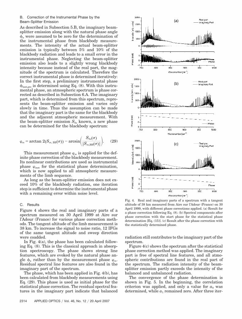
Figure 4 shows the real and imaginary parts of aspectrum measured on 30 April 1999 at Aire surl’Adour (France) for various phase correction meth-ods. The tangent altitude of the limb measurement is38 km. To increase the signal to noise ratio, 12 IFGsof the same tangent altitude and sweep directionwere coadded.
In Fig. 4(a), the phase has been calculated follow-ing Eq. (8). This is the classical approach in absorp-tion spectroscopy. The phase shows strong linefeatures, which are evoked by the natural phase an-gle �n rather than by the measurement phase m.Residual spectral line features are also found in theimaginary part of the spectrum.
The phase, which has been applied in Fig. 4(b), hasbeen calculated from blackbody measurements usingEq. (29). This phase is used as initial phase for thestatistical phase correction. The residual spectral fea-tures in the imaginary part indicate that balanced
radiation still contributes to the imaginary part of thespectrum.
Figure 4(c) shows the spectrum after the statisticalphase correction method was applied. The imaginarypart is free of spectral line features, and all atmo-spheric contributions are found in the real part ofthe spectrum. The radiation intensity of the beam-splitter emission partly exceeds the intensity of thebalanced and unbalanced radiation.
The convergence of the phase determination isshown in Fig. 5. In the beginning, the correlationcriterion was applied, and only a value for a0 wasdetermined, while a1 remained zero. After three iter-
Fig. 4. Real and imaginary parts of a spectrum with a tangentaltitude of 38 km measured from Aire sur l’Adour (France) on 30April 1999, with different phase corrections applied. (a) Result fora phase correction following Eq. (8). (b) Spectral components afterphase correction with the start phase for the statistical phasedetermination [Eq. (15)]. (c) Result after the phase correction withthe statistically determined phase.
ations, a0,n has become zero, and the phase determi-nation process switched to the variance criterion.Convergence was reached after approximately 13steps, where the iterative values of a0 and a1 rapidlydecreased by approximately 3 orders of magnitude. Inthe further iterations, a0 and a1 oscillate around zero.In the plot, only the absolute values are displayed toallow for a logarithmic scale.
7. Error Estimation
The error analysis for the phase determination is doneexemplarily for the long wavelength range �750–1000cm�1�. Owing to the relatively strong beam-splitteremission in this spectral region, this range is mostsensitive to phase errors. The errors that contributeto the correction of the instrumental phase and thelinear phase are analyzed separately.
A. Error of the Instrumental Phase
Three sources of uncertainties have to be considered:
Y Noise in the blackbody measurements.Y Time-dependent drift of the instrumental phase
between subsequent blackbody measurements.Y Inaccuracies in the determination of the beam-
splitter emission.
The error attributable to noise is calculated withthe standard error propagation formulas. Three in-dependent noise contributions have to be considered:noise in the real part of the blackbody spectrumRe�Sm,BB�, noise in the imaginary part of the black-body spectrum Im�Sm,BB�, and noise in the beam-splitter spectrum �Sbs�, which is the imaginary part ofan atmospheric spectrum. The noise amplitudes areconsidered the same in all three cases and are de-noted as �S. The phase error � is calculated as
��inst,noise�2 � � �inst
� Re�Sm,BB��S�2
� �inst
� Im�Sm,BB��S�2
� �inst
��Sbs��S�2
. (30)
The error attributable to the noise of the instrumen-tal phase inst is the same as for the phase m in Eq.(29) because the only difference between these twoterms is a straight line, which is noise free. BecauseSbs � 0.2|Sm,BB|, the approximation
arcsin� Sbs����Sm,BB������
Sbs����Sm,BB����
(31)
can be made for the error estimation. Using the re-lation Sm,BB
2 � Re�Sm,BB�2 Im�Sm,BB�2, the error isgiven as
��inst,noise� ��S
�Sm,BB��1 1 �4Sbs
�Sm,BB�Ç
�0.2
Re�Sm,BB��Sm,BB�Ç
�1
�Im�Sm,BB��Sm,BB�Ç
�1
� Sbs
Sm,BB�2
�0.2
��1�2
. (32)
The term in the squared brackets is smaller than 3,therefore the upper limit of the error in the instru-mental phase due to noise is given as
��inst,noise� � 3�S
�Sm,BB�. (33)
The spectral resolution of the blackbody spectrumand the beam-splitter spectrum has been reduced to1�15th of the full resolution to calculate the instru-mental phase (see also Subsection 5.B). Therefore thenoise �S is reduced by a factor of 15 compared to thefull resolution.
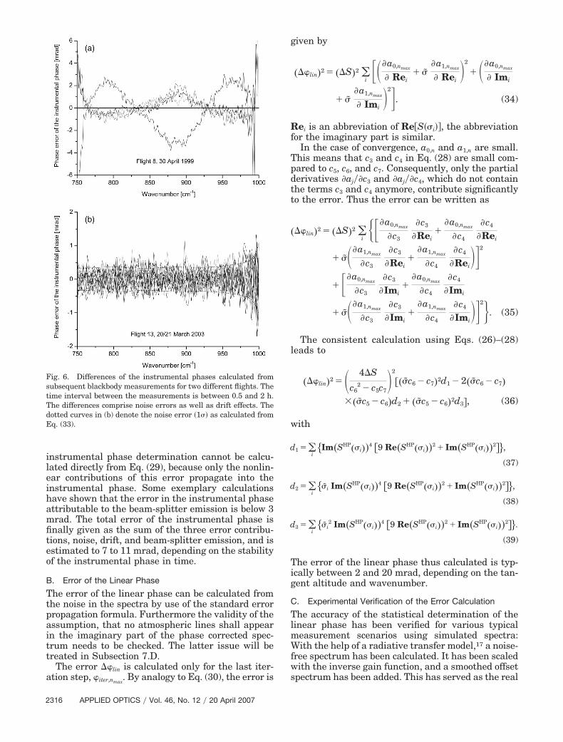
The error attributable to the drift of the instrumen-tal phase between subsequent blackbody measure-ments is given by the difference of the nonlinearcontributions of the blackbody phases. In some flightsthere are systematic differences between two subse-quent instrumental phase spectra, whereas in otherflights only noise is visible. Figure 6 shows the dif-ferences of subsequent instrumental phase spectrafor (a) flight 8 on 30 April 1999 and (b) flight 13 on20�21 March 2003. In flight 8, systematic deviationsof approximately 4 mrad are visible (in this flightthe beam-splitter unit showed a thermally inducedmechanical instability). In flight 13 the phase dif-ferences between the two blackbody measurementsdo not exceed the noise level. The dotted curvesindicate the noise error �1��, which is calculatedusing Eq. (33).
The beam-splitter emission Sbs is determined froman atmospheric spectrum using the statistical phasedetermination. Consequently, the error in the statis-tical phase determination as well as the drift effectsin time between the blackbody measurement and theatmospheric measurement have to be considered aserror sources for Sbs. The analysis of various balloonflights has shown that the accuracy of Sbs can beestimated to 5%. The impact of this error on the
Fig. 5. Evolution of the offset a0 (triangles) and the slope a1
(squares) during the iterations of the statistical phase determina-tion. The absolute values of a0 and a1 are displayed to allow for alogarithmic scale. At the third iteration step, a0 equals zero and istherefore not displayed in the logarithmic plot.
instrumental phase determination cannot be calcu-lated directly from Eq. (29), because only the nonlin-ear contributions of this error propagate into theinstrumental phase. Some exemplary calculationshave shown that the error in the instrumental phaseattributable to the beam-splitter emission is below 3mrad. The total error of the instrumental phase isfinally given as the sum of the three error contribu-tions, noise, drift, and beam-splitter emission, and isestimated to 7 to 11 mrad, depending on the stabilityof the instrumental phase in time.
B. Error of the Linear Phase
The error of the linear phase can be calculated fromthe noise in the spectra by use of the standard errorpropagation formula. Furthermore the validity of theassumption, that no atmospheric lines shall appearin the imaginary part of the phase corrected spec-trum needs to be checked. The latter issue will betreated in Subsection 7.D.
The error �lin is calculated only for the last iter-ation step, iter,nmax
. By analogy to Eq. (30), the error is
given by
��lin�2 � ��S�2 i���a0,nmax
� Rei �̃
�a1,nmax
� Rei�2
��a0,nmax
� Imi
�̃�a1,nmax
� Imi�2�. (34)
Rei is an abbreviation of Re�S��i��, the abbreviationfor the imaginary part is similar.
In the case of convergence, a0,n and a1,n are small.This means that c3 and c4 in Eq. (28) are small com-pared to c5, c6, and c7. Consequently, only the partialderivatives �aj��c3 and �aj��c4, which do not containthe terms c3 and c4 anymore, contribute significantlyto the error. Thus the error can be written as
��lin�2 � ��S�2 i���a0,nmax
�c3
�c3
�Rei
�a0,nmax
�c4
�c4
�Rei
�̃��a1,nmax
�c3
�c3
�Rei
�a1,nmax
�c4
�c4
�Rei��2
��a0,nmax
�c3
�c3
�Imi
�a0,nmax
�c4
�c4
�Imi
�̃��a1,nmax
�c3
�c3
�Imi
�a1,nmax
�c4
�c4
�Imi��2�. (35)
The consistent calculation using Eqs. (26)–(28)leads to
The error of the linear phase thus calculated is typ-ically between 2 and 20 mrad, depending on the tan-gent altitude and wavenumber.
C. Experimental Verification of the Error Calculation
The accuracy of the statistical determination of thelinear phase has been verified for various typicalmeasurement scenarios using simulated spectra:With the help of a radiative transfer model,17 a noise-free spectrum has been calculated. It has been scaledwith the inverse gain function, and a smoothed offsetspectrum has been added. This has served as the real
Fig. 6. Differences of the instrumental phases calculated fromsubsequent blackbody measurements for two different flights. Thetime interval between the measurements is between 0.5 and 2 h.The differences comprise noise errors as well as drift effects. Thedotted curves in (b) denote the noise error �1�� as calculated fromEq. (33).
part of the simulated, uncalibrated spectrum. A mea-sured and smoothed beam-splitter emission spec-trum has been used as the imaginary part. Thesimulated complex spectrum has been Fourier trans-formed into an IFG to which a random noise corre-sponding to the noise of the measurement has beenadded. In analogy to a Monte Carlo simulation, a dataset of 50 IFGs has been generated. These IFGs havethen been phase corrected with the statistical phasecorrection method described above. The error of thephase correction has been calculated according to Eq.(35). This error has then been compared to the resid-ual phase error of the simulated spectra of the MonteCarlo simulation. An example of this analysis isshown in Fig. 7. The simulated spectra correspond toa single deep-space spectrum as measured in midlati-tudes from a flight altitude of 38 km. The residualphase errors after phase correction show a statisticalbehavior, and the mean residual phase error (thickline) is close to zero. The standard deviation �1�� isgiven by the dashed black lines. The solid black linesshow the error of the linear phase as calculated usingerror propagation. The order of magnitude and theshape of the residual phase error are well represent-ed; however, the value of the residual error is under-estimated by a factor of 1.6 to 1.8. Since the errorpropagation calculation is based on a linear approx-imation, such a deviation is not too astonishing. Thesimulation has been performed for various situations,i.e., different atmospheric signals (high and low at-mosphere, arctic and midlatitude situations) and dif-ferent noise levels. In all cases, the ratio between thereal phase error and the calculated phase error hasbeen between 0.9 and 1.8, therefore the error calcu-lated from error propagation is multiplied by a factorof 2 to give a reasonable worst case estimation of theerror. Hence, the error of the statistical determina-tion of the linear phase is given as
��lin�2 � 2� 4�S
c62 � c5c7
�2
���̃c6 � c7�2d1 � 2��̃c6 � c7�
� ��̃c5 � c6�d2 ��̃c5 � c6�2d3�. (40)
With this estimation, the error of the linear phaseranges from 10 to 20 mrad, depending on the wave-number. For lower tangent altitudes, the uncertaintyis smaller because of the higher signal to noise ratio.For the lowermost tangent altitude, this error is be-low 5 mrad for a single spectrum. It decreases more orless linearly with the noise level, therefore the co-adding of the IFGs also reduces the error.
D. Validity of the Assumptions Made
The validity of the assumption that no atmosphericlines shall appear in the imaginary part of the phasecorrected spectrum needs to be evaluated with re-spect to beam-splitter absorption and with respect tospectral features attributable to emitting and absorb-ing gas in the instrument. Beam-splitter absorptionleads to additional phase angles u and bs (see Sec-tion 3). Some emitting and absorbing gas in the in-strument leads to the following effects:
Y The radiation emitted by the beam splitter ispartly absorbed by the gas between the beam splitterand the detector. Thus the beam splitter spectrumshows some absorption lines.
Y The thermal emission of the gas between thebeam splitter and the detector against the cold detec-tor leads to emission lines in the unbalanced beam.
Four combinations of beam-splitter absorption andgas in the instrument have to be considered in themeasured spectral interval:
1. There is no beam-splitter absorption, and theinstrument is free of any gases.
2. There is a significant beam-splitter absorption,and the instrument is free of any gases.
3. There is no beam-splitter absorption, and theinstrument contains some gases.
4. There is a significant beam-splitter absorption,and the instrument contains some gases.
In the first case, the assumption of no atmosphericlines in the imaginary part is correct since the phaserelation between the balanced port and the beam-splitter port is exactly ��2, and the relation betweenthe balanced and the unbalanced port is exactly �.Furthermore all atmospheric radiation comes fromoutside the instrument and belongs to the balancedport.
In the second case, the beam-splitter absorptionleads to additional phase angles u and bs. The effectof these angles is that a part of the beam-splitterradiation is mapped to the real part of the spectrumwhereas a part of the unbalanced radiation ismapped to the imaginary part of the spectrum. Sinceboth contributions are free of spectral lines, the imag-inary part is still free of line features. The part of thebeam-splitter emission, which is mapped to the real
Fig. 7. Error of the statistical phase determination as deter-mined by a Monte Carlo simulation with 50 spectra. The meanresidual phase error (thick solid line) is close to zero. The blackdashed lines show the standard deviation of the residual phaseerror �1��. The black straight lines show the error of the statis-tical phase determination �1�� as calculated from error propa-gation [Eq. (36)].
part of the spectrum, is removed during calibration,together with the other radiation contributions of theinstrument.
In the third case, the beam-splitter spectrum is zeroand thus cannot contain spectral features because ofinternal absorption. The additional phase angles u
and bs are also zero, therefore the radiation of theunbalanced beam is mapped entirely on the (nega-tive) real axis. The radiation of the balanced beam ismapped on the real axis anyhow. Consequently, theassumption is also fulfilled in this case.
In the last case, the beam-splitter spectrum showsabsorption lines and the unbalanced port containsemission lines of the internal gas. Since the addi-tional phase angles u and bs are different from zero,a part of the unbalanced port (containing spectrallines) is mapped to the imaginary part of the spec-trum. If beam-splitter absorption and line features inthe instrument occur in the same spectral range, thepresented method here may lead to noticeable phaseerrors. The magnitude of this error depends on theline intensities and the strength of the beam-splitterabsorption.
In the case of MIPAS-B2, some water vapor linesoriginating from gas in the instrument are found inthe spectral channel covering the range of 1557 to1774 cm�1. Within this channel, the beam-splitteremission is below 1%, and test calculations with sim-ulated spectra have shown that the line features inthe imaginary part are well below the noise level. Thephase error introduced by these lines is approxi-mately 1 mrad and thus below the statistical error ofthe linear phase.
E. Overall Phase Error
The overall phase error is given as the sum of theerror of the instrumental phase and of the linearphase. With the estimations given above, the overallerror is in the range of 9 to 31 mrad, depending on thestability of the instrumental phase, the intensity ofthe atmospheric signal, and the number of coaddi-tions.
F. Impact on the Calibrated Spectrum
In the case of a residual phase error that is not cor-rected a part of the balanced and unbalanced radiationis turned into the imaginary part of the spectrum, anda part of the beam-splitter emission shows up in thereal part
For small values of �, only the baseline of the spec-trum is affected by the beam-splitter emission, whilethe line intensities remain unchanged. The only im-pact on the line intensities originates from phaseerrors in the blackbody and deep-space spectra,which are used for calibration. This scaling error ofthe spectrum is below 0.1%. The error in the baselineattributable to an imperfect phase correction has
been estimated to less than 4 nW��cm2 sr cm�1�. Thisis of the order of the noise level of a single spectrum.10
Hence the error in the phase determination usuallyhas no significant impact anymore on the accuracy ofthe calibrated spectra.
8. Conclusions
A new method for the phase correction of interfero-grams in emission spectroscopy has been developed.The method presented of a statistical approach todetermine the measurement phase allows us to sep-arate the spectral components of balanced and un-balanced radiation from beam-splitter emission forindividual spectra, provided that the instrumentalradiation contains no high-resolution features in thespectral range where beam-splitter emission occurs.This method is suited for situations where phasedrifts occur (e.g., due to thermal drift) and providesgood results even in the case of low signal radiation.
In the MIPAS-B2 experiment, it has become pos-sible with this method to correct the measurementphase resulting from the optical components, theelectrical delay times of the amplifiers, and the dis-crete sampling. Meanwhile, the method describedhere has been applied to many flights performed withMIPAS-B2 under various conditions. It was also ap-plied to the airborne MIPAS-STR instrument on Geo-physica. The phase correction works properly in mostsituations and can be applied to all elevation angles.Only in situations with a very poor signal-to-noiseratio (e.g., extremely cold atmosphere), the methodmay be inadequate. Such a situation has occurredonly once in 15 balloon flights and has affected onlythe deep-space spectra. In this case, the phase stabil-ity has been proven to be good enough that the phaseof adjacent measurements with a stronger atmo-spheric signal could be used.
The method presented here has the advantage thatthe accuracy of the phase determination can easily becalculated for each individual spectrum, which en-sures a reliable and continuous data quality check.The phase correction approach together with the de-termination of its accuracy has been successfully val-idated with a Monte Carlo approach. The quality ofthe phase determination method is sufficient to re-duce the error in the calibrated spectrum attributableto residual phase errors to or below the level of thephoton noise. Thus the phase determination issue issolved for the MIPAS-B2 experiment.
The authors thank the members of the Institut fürMeteorologie und Klimaforschung and the team ofthe MIPAS-B2 experiment for the friendly atmo-sphere and stimulating discussions. This work wassupported by the Forschungszentrum Karlsruhe,Germany.
References1. L. Mertz, Transformations in Optics (Wiley, 1965).2. M. L. Forman, W. H. Steel, and G. Vanasse, “Correction of
Smith, and L. Sromovsky, “Radiometric calibration of IR Fou-rier transform spectrometers: solution to a problem with thehigh-resolution interferometer sounder,” Appl. Opt. 27, 3210–3218 (1988).
4. C. E. Blom, M. Höpfner, and Ch. Weddigen, “Correction ofphase anomalies of atmospheric emission spectra by thedouble-differencing method,” Appl. Opt. 35, 2649–2652 (1996).
5. D. G. Johnson, W. A. Traub, and K. W. Jucks, “Phase deter-mination from mostly one-sided interferograms,” Appl. Opt.35, 2955–2959 (1996).
6. G. Wetzel, H. Oelhaf, R. Ruhnke, F. Friedl-Vallon, A. Kleinert,W. Kouker, G. Maucher, Th. Reddmann, M. Seefeldner, M.Stowasser, O. Trieschmann, T. von Clarmann, and H. Fischer,“NOy partitioning and budget and its correlation with N2O inthe Arctic vortex and in summer midlatitudes in 1997,” J. Geo-phys. Res. 107, 4280–4290, 10.1029/2001JD000916 (2002).
7. M. Stowasser, H. Oelhaf, R. Ruhnke, A. Kleinert, G. Wetzel, F.Friedl-Vallon, W. Kouker, A. Lengel, G. Maucher, H. Nordm-eyer, Th. Reddmann, and H. Fischer, “The variation of short-lived NOy species around sunrise at midlatitudes as measuredby MIPAS-B and calculated by KASIMA,” Geophys. Res. Lett.30, 1432–1436 (2003).
8. G. Wetzel, H. Oelhaf, F. Friedl-Vallon, A. Kleinert, A. Lengel,G. Maucher, H. Nordmeyer, R. Ruhnke, H. Nakajima, Y.Sasano, T. Sugita, and T. Yokota, “Intercomparison and vali-dation of ILAS-II version 1.4 target parameters with MIPAS-Bmeasurements,” J. Geophys. Res. 111, 10.1029/2005JD006287(2006).
9. H. Oelhaf, F. Friedl-Vallon, A. Kleinert, A. Lengel, G.Maucher, H. Nordmeyer, G. Wetzel, G. Zhang, and H. Fischer,“ENVISAT validation with MIPAS-B,” in Proceedings of the En-visat Validation Workshop, ESA SP-531 H. Sawaya- Lacoste, ed.
(European Space Agency, 2003), http://envisat.esa.int/pub/ESA_DOC/envisat_val_1202/proceedings/ACV/balloon/02_oelhaf.pdf.
10. F. Friedl-Vallon, G. Maucher, A. Kleinert, A. Lengel, C. Keim,H. Oelhaf, H. Fischer, M. Seefeldner, and O. Trieschmann,“Design and characterization of the balloonborne Michelsoninterferometer for passive atmospheric sounding (MIPAS-B2),”Appl. Opt. 43, 3335–3355 (2004).
11. A. A. Michelson, Light Waves and Their Uses (University ofChicago Press, 1902).
12. Ch. Weddingen, C. E. Blom, and M. Höpfner, “Phase correctionfor the emission sounder MIPAS-FT,” Appl. Opt. 32, 4586–4589 (1993).
14. O. Trieschmann and Ch. Weddigen, “Thermal emission fromdielectric beam splitters in Michelson interferometers: A sche-matic analysis,” Appl. Opt. 39, 5834–5842 (2000).
15. F. Hase, O. Trieschmann, and Ch. Weddigen, “Response ofFourier-transform spectrometers to absorption and emissionin a homogeneous single-layer beam splitter,” Appl. Opt. 40,5078–5087 (2001).
16. B. Carli, L. Palchetti, and P. Raspollini, “Effect of beam-splitter emission in Fourier transform spectroscopy,” Appl.Opt. 38, 74757480 (1999).
17. G. P. Stiller, ed., with contributions from T. v. Clarmann, A.Dudhia, G. Echle, B. Funke, N. Glatthor, F. Hase, M. Höpfner,S. Kellmann, H. Kemnitzer, M. Kuntz, A. Linden, M. Linder,G. P. Stiller, and S. Zorn, “The Karlsruhe optimized and pre-cise radiative transfer algorithm (KOPRA),” WissenschaftlicheBerichte des Forschungszentrums Karlsruhe, FZKA 6487(Karlsruhe, 2000).