126
Phased Scheduling of Stream Programs Michal Karczmarek, William Thies and Saman Amarasinghe MIT LCS
| Date post: | 02-Jan-2016 |
| Category: |
Documents |
| Upload: | risa-guerrero |
| View: | 17 times |
| Download: | 0 times |

Phased Schedulingof Stream Programs
Michal Karczmarek, William Thies
and Saman Amarasinghe
MIT LCS
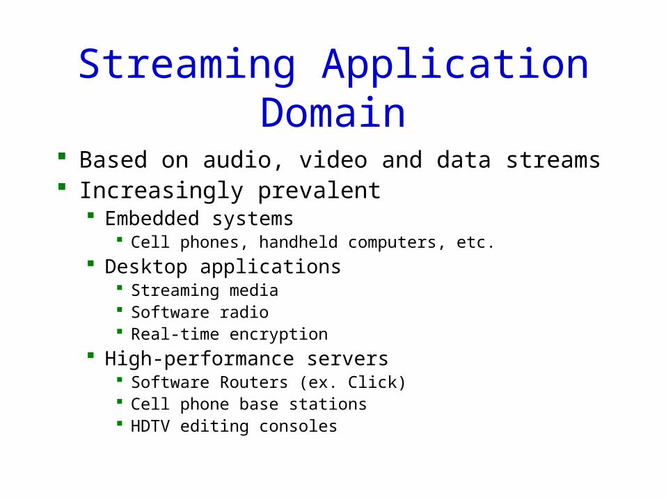
Streaming Application Domain
Based on audio, video and data streams Increasingly prevalent
Embedded systems Cell phones, handheld computers, etc.
Desktop applications Streaming media Software radio Real-time encryption
High-performance servers Software Routers (ex. Click) Cell phone base stations HDTV editing consoles

Properties of Stream Programs
A large (possibly infinite) amount of data Limited lifespan of each data item Little processing of each data item
A regular, static computation pattern Stream program structure is relatively constant A lot of opportunities for compiler
optimizations

StreamIt Language
Streaming Language from MIT LCS Similar to Synchronous Data Flow
(SDF) Provides hierarchy & structure Four Structures:
Filter Pipeline SplitJoin FeedbackLoop
All Structures have Single-Input Channel Single-Output Channel
Filters allow ‘peeking’ – looking at items which are not consumed
Splitter
LPF
CClip
ACorr
Sink
Joiner
Source
LPF
HPF
Compress
LPF
HPF
Compress
LPF
HPF
Compress
LPF
HPF
Compress

Our Contributions
New scheduling technique called Phased Scheduling
Small buffer sizes for hierarchical programs Fine grained control over schedule size vs buffer
size tradeoff Allows for separate compilation by always
avoiding deadlock Performs initialization for peeking Filters

Overview
General Stream Concepts StreamIt Details Program Steady State and Initialization Single Appearance and Pull Scheduling Phased Scheduling
Minimal Latency
Results Related Work and Conclusion

Stream Programs
Consist of Filters and Channels Filters perform computation Channels act as FIFO queues
for data between Filters
filter
filter
filter
filter

Filters
Execute a work function which: Consumes data from their input Produces data to their output
Filters consume and produce constant amount of data on every execution of the work function Rates are known at compilation time
Filter executions are atomic
filter

Stream Program Schedule
Describes the order in which filters are executed
Needs to manage grossly mismatched rates between filters
Manages data buffered up in channels between filters
Controls latency of data processing

Overview
General Stream Concepts StreamIt Details Program Steady State and Initialization Single Appearance and Pull Scheduling Phased Scheduling
Minimal Latency
Results Related Work and Conclusion

StreamIt - Filter
Performs the computation Consumes pop data items Produces push data items Inspects peek data items
peek, pop
push
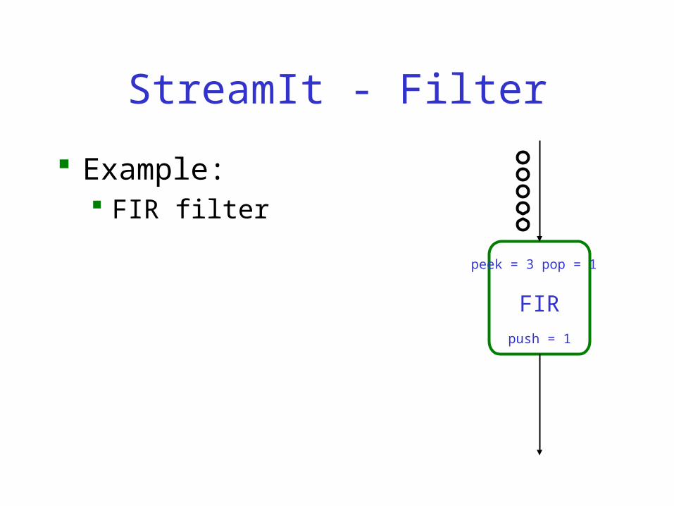
StreamIt - Filter
Example: FIR filter
peek = 3 pop = 1
FIR
push = 1

StreamIt - Filter
Example: FIR filter Inspects 3 data items
peek = 3 pop = 1
FIR
push = 1

StreamIt - Filter
Example: FIR filter Inspects 3 data items Consumes 1 data item
peek = 3 pop = 1
FIR
push = 1

StreamIt - Filter
Example: FIR filter Inspects 3 data items Consumes 1 data item Produces 1 data item
peek = 3 pop = 1
FIR
push = 1

StreamIt - Filter
Example: FIR filter Inspects 3 data items Consumes 1 data item Produces 1 data item
peek = 3 pop = 1
FIR
push = 1

StreamIt - Filter
Example: FIR filter Inspects 3 data items Consumes 1 data item Produces 1 data item And again…
peek = 3 pop = 1
FIR
push = 1

StreamIt - Filter
Example: FIR filter Inspects 3 data items Consumes 1 data item Produces 1 data item And again…
peek = 3 pop = 1
FIR
push = 1

StreamIt - Filter
Example: FIR filter Inspects 3 data items Consumes 1 data item Produces 1 data item And again…
peek = 3 pop = 1
FIR
push = 1

StreamIt - Filter
Example: FIR filter Inspects 3 data items Consumes 1 data item Produces 1 data item And again…
peek = 3 pop = 1
FIR
push = 1

StreamIt - Filter
Example: FIR filter Inspects 3 data items Consumes 1 data item Produces 1 data item And again…
peek = 3 pop = 1
FIR
push = 1
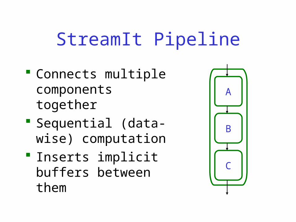
StreamIt Pipeline
Connects multiple components together
Sequential (data-wise) computation
Inserts implicit buffers between them
A
B
C

StreamIt SplitJoin
Also connects several components together
Parallel computation construct
Allows for computation of same data (DUPLICATE splitter) or different data (ROUND_ROBIN splitter)
BA
splitter
joiner

StreamIt FeedbackLoop
ONLY structure to allow data cycles
Needs initialization on feedbackPath
Amount of data on feedbackPath is delay
B L
splitter
joiner
delay

Overview
General Stream Concepts StreamIt Details Program Steady State and Initialization Single Appearance and Pull Scheduling Phased Scheduling
Minimal Latency
Results Related Work and Conclusion

Scheduling – Steady State
Every valid stream graph has a Steady State Steady State does not change amount of
data buffered between components Steady State can be executed repeatedly
forever without growing buffers

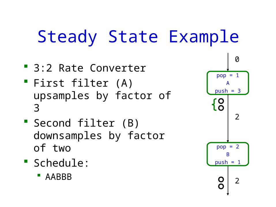
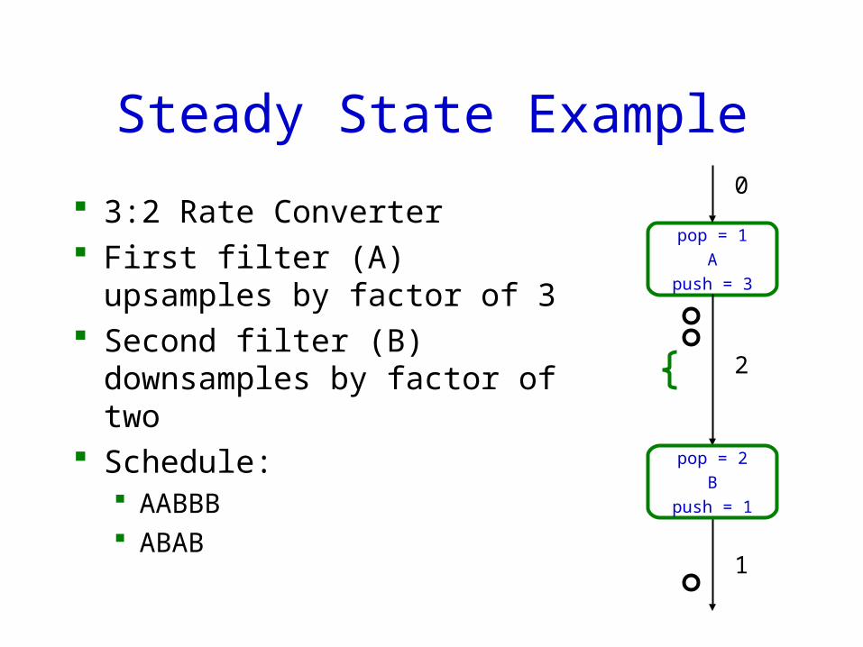
Steady State Example
3:2 Rate Converter First filter (A) upsamples by
factor of 3 Second filter (B)
downsamples by factor of 2
pop = 1
A
push = 3
pop = 2
B
push = 1

Steady State Example
A executes 2 times pushes 2 * 3 = 6 items
B executes 3 times pops 3 * 2 = 6 items
Number of data items stored between Filters does not change
pop = 1
A
push = 3
pop = 2
B
push = 1
2 *
3 *

Steady State Example
3:2 Rate Converter First filter (A) upsamples by
factor of 3 Second filter (B) downsamples
by factor of two Schedule:
pop = 1
A
push = 3
pop = 2
B
push = 1
2
0
0

Steady State Example
3:2 Rate Converter First filter (A) upsamples by
factor of 3 Second filter (B) downsamples
by factor of two Schedule:
A
pop = 1
A
push = 3
pop = 2
B
push = 1
2
0
0

Steady State Example
3:2 Rate Converter First filter (A) upsamples by
factor of 3 Second filter (B) downsamples
by factor of two Schedule:
A
pop = 1
A
push = 3
pop = 2
B
push = 1
1
0
0

Steady State Example
3:2 Rate Converter First filter (A) upsamples by
factor of 3 Second filter (B) downsamples
by factor of two Schedule:
A
pop = 1
A
push = 3
pop = 2
B
push = 1
1
3
0

Steady State Example
3:2 Rate Converter First filter (A) upsamples by
factor of 3 Second filter (B) downsamples
by factor of two Schedule:
AA
pop = 1
A
push = 3
pop = 2
B
push = 1
1
3
0

Steady State Example
3:2 Rate Converter First filter (A) upsamples by
factor of 3 Second filter (B) downsamples
by factor of two Schedule:
AA
pop = 1
A
push = 3
pop = 2
B
push = 1
0
3
0

Steady State Example
3:2 Rate Converter First filter (A) upsamples by
factor of 3 Second filter (B) downsamples
by factor of two Schedule:
AA
pop = 1
A
push = 3
pop = 2
B
push = 1
0
6
0

Steady State Example
3:2 Rate Converter First filter (A) upsamples by
factor of 3 Second filter (B) downsamples
by factor of two Schedule:
AAB
pop = 1
A
push = 3
pop = 2
B
push = 1
0
6
0

Steady State Example
3:2 Rate Converter First filter (A) upsamples by
factor of 3 Second filter (B) downsamples
by factor of two Schedule:
AAB
pop = 1
A
push = 3
pop = 2
B
push = 1
0
4
0

Steady State Example
3:2 Rate Converter First filter (A) upsamples by
factor of 3 Second filter (B) downsamples
by factor of two Schedule:
AAB
pop = 1
A
push = 3
pop = 2
B
push = 1
0
4
1

Steady State Example
3:2 Rate Converter First filter (A) upsamples by
factor of 3 Second filter (B) downsamples
by factor of two Schedule:
AABB
pop = 1
A
push = 3
pop = 2
B
push = 1
0
4
1

Steady State Example
3:2 Rate Converter First filter (A) upsamples by
factor of 3 Second filter (B) downsamples
by factor of two Schedule:
AABB
pop = 1
A
push = 3
pop = 2
B
push = 1
0
2
1

Steady State Example
3:2 Rate Converter First filter (A) upsamples by
factor of 3 Second filter (B) downsamples
by factor of two Schedule:
AABB
pop = 1
A
push = 3
pop = 2
B
push = 1
0
2
2
Steady State Example
3:2 Rate Converter First filter (A) upsamples by
factor of 3 Second filter (B) downsamples
by factor of two Schedule:
AABBB
pop = 1
A
push = 3
pop = 2
B
push = 1
0
2
2

Steady State Example
3:2 Rate Converter First filter (A) upsamples by
factor of 3 Second filter (B) downsamples
by factor of two Schedule:
AABBB
pop = 1
A
push = 3
pop = 2
B
push = 1
0
0
2

Steady State Example
3:2 Rate Converter First filter (A) upsamples by
factor of 3 Second filter (B) downsamples
by factor of two Schedule:
AABBB
pop = 1
A
push = 3
pop = 2
B
push = 1
0
0
3

Steady State Example
3:2 Rate Converter First filter (A) upsamples by
factor of 3 Second filter (B) downsamples
by factor of two Schedule:
AABBB
pop = 1
A
push = 3
pop = 2
B
push = 1
0
0
3

Steady State Example
3:2 Rate Converter First filter (A) upsamples by
factor of 3 Second filter (B) downsamples
by factor of two Schedule:
AABBB A
pop = 1
A
push = 3
pop = 2
B
push = 1
2
0
0

Steady State Example
3:2 Rate Converter First filter (A) upsamples by
factor of 3 Second filter (B) downsamples
by factor of two Schedule:
AABBB A
pop = 1
A
push = 3
pop = 2
B
push = 1
1
0
0

Steady State Example
3:2 Rate Converter First filter (A) upsamples by
factor of 3 Second filter (B) downsamples
by factor of two Schedule:
AABBB A
pop = 1
A
push = 3
pop = 2
B
push = 1
1
3
0

Steady State Example
3:2 Rate Converter First filter (A) upsamples by
factor of 3 Second filter (B) downsamples
by factor of two Schedule:
AABBB AB
pop = 1
A
push = 3
pop = 2
B
push = 1
1
3
0

Steady State Example
3:2 Rate Converter First filter (A) upsamples by
factor of 3 Second filter (B) downsamples
by factor of two Schedule:
AABBB AB
pop = 1
A
push = 3
pop = 2
B
push = 1
1
1
0

Steady State Example
3:2 Rate Converter First filter (A) upsamples by
factor of 3 Second filter (B) downsamples
by factor of two Schedule:
AABBB AB
pop = 1
A
push = 3
pop = 2
B
push = 1
1
1
1

Steady State Example
3:2 Rate Converter First filter (A) upsamples by
factor of 3 Second filter (B) downsamples
by factor of two Schedule:
AABBB ABA
pop = 1
A
push = 3
pop = 2
B
push = 1
1
1
1

Steady State Example
3:2 Rate Converter First filter (A) upsamples by
factor of 3 Second filter (B) downsamples
by factor of two Schedule:
AABBB ABA
pop = 1
A
push = 3
pop = 2
B
push = 1
0
1
1

Steady State Example
3:2 Rate Converter First filter (A) upsamples by
factor of 3 Second filter (B) downsamples
by factor of two Schedule:
AABBB ABA
pop = 1
A
push = 3
pop = 2
B
push = 1
0
4
1

Steady State Example
3:2 Rate Converter First filter (A) upsamples by
factor of 3 Second filter (B) downsamples
by factor of two Schedule:
AABBB ABAB
pop = 1
A
push = 3
pop = 2
B
push = 1
0
4
1
Steady State Example
3:2 Rate Converter First filter (A) upsamples by
factor of 3 Second filter (B) downsamples
by factor of two Schedule:
AABBB ABAB
pop = 1
A
push = 3
pop = 2
B
push = 1
0
2
1

Steady State Example
3:2 Rate Converter First filter (A) upsamples by
factor of 3 Second filter (B) downsamples
by factor of two Schedule:
AABBB ABAB
pop = 1
A
push = 3
pop = 2
B
push = 1
0
2
2

Steady State Example
3:2 Rate Converter First filter (A) upsamples by
factor of 3 Second filter (B) downsamples
by factor of two Schedule:
AABBB ABABB
pop = 1
A
push = 3
pop = 2
B
push = 1
0
2
2

Steady State Example
3:2 Rate Converter First filter (A) upsamples by
factor of 3 Second filter (B) downsamples
by factor of two Schedule:
AABBB ABABB
pop = 1
A
push = 3
pop = 2
B
push = 1
0
0
2

Steady State Example
3:2 Rate Converter First filter (A) upsamples by
factor of 3 Second filter (B) downsamples
by factor of two Schedule:
AABBB ABABB
pop = 1
A
push = 3
pop = 2
B
push = 1
0
0
3

Steady State Example
3:2 Rate Converter First filter (A) upsamples by
factor of 3 Second filter (B) downsamples
by factor of two Schedule:
AABBB ABABB
pop = 1
A
push = 3
pop = 2
B
push = 1
0
0
3

Steady State Example - Buffers
AABBB requires 6 data items of buffer space between filters A and B
ABABB requires 4 data items of buffer space between filters A and B
pop = 1
A
push = 3
pop = 2
B
push = 1
0
0
3

Steady State Example - Latency
AABBB – First data item output after third execution of an filter Also A already consumed 2
data items ABABB – First data item
output after second execution of an filter A consumed only 1 data item
pop = 1
A
push = 3
pop = 2
B
push = 1
0
0
3

Initialization
Filter Peeking provides a new challenge
Just Steady State doesn’t work:
pop = 1
A
push = 3
peek = 3, pop = 2
B
push = 1
3
0
0

Initialization
Filter Peeking provides a new challenge
Just Steady State doesn’t work: A
pop = 1
A
push = 3
peek = 3, pop = 2
B
push = 1
2
3
0

Initialization
Filter Peeking provides a new challenge
Just Steady State doesn’t work: AA
pop = 1
A
push = 3
peek = 3, pop = 2
B
push = 1
1
6
0

Initialization
Filter Peeking provides a new challenge
Just Steady State doesn’t work: AAB
pop = 1
A
push = 3
peek = 3, pop = 2
B
push = 1
1
4
1

Initialization
Filter Peeking provides a new challenge
Just Steady State doesn’t work: AABB Can’t execute B again!
pop = 1
A
push = 3
peek = 3, pop = 2
B
push = 1
1
2
2

Initialization
Filter Peeking provides a new challenge
Just Steady State doesn’t work: AABB Can’t execute B again!
Can’t execute A one extra time: AABB
pop = 1
A
push = 3
peek = 3, pop = 2
B
push = 1
1
2
2

Initialization
Filter Peeking provides a new challenge
Just Steady State doesn’t work: AABB Can’t execute B again!
Can’t execute A one extra time: AABBA
pop = 1
A
push = 3
peek = 3, pop = 2
B
push = 1
0
5
2

Initialization
Filter Peeking provides a new challenge
Just Steady State doesn’t work: AABB Can’t execute B again!
Can’t execute A one extra time: AABBAB Left 3 items between A and B!
pop = 1
A
push = 3
peek = 3, pop = 2
B
push = 1
0
3
3

Initialization
Must have data between A and B before starting execution of Steady State Schedule
Construct two schedules: One for Initialization One for Steady State
Initialization Schedule leaves data in buffers so Steady State can execute
pop = 1
A
push = 3
peek = 3, pop = 2
B
push = 1
0
3
3
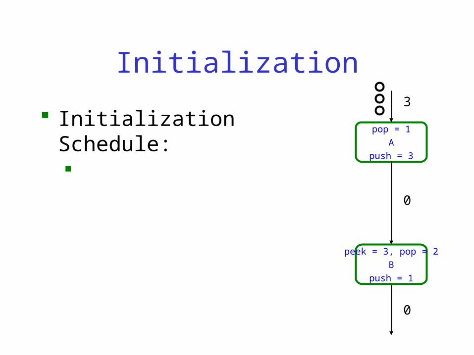
Initialization
Initialization Schedule:
pop = 1
A
push = 3
peek = 3, pop = 2
B
push = 1
3
0
0

Initialization
Initialization Schedule: A
pop = 1
A
push = 3
peek = 3, pop = 2
B
push = 1
2
3
0

Initialization
Initialization Schedule: A Leave 3 items between A and B
Steady State Schedule:
pop = 1
A
push = 3
peek = 3, pop = 2
B
push = 1
2
3
0

Initialization
Initialization Schedule: A Leave 3 items between A and B
Steady State Schedule: A
pop = 1
A
push = 3
peek = 3, pop = 2
B
push = 1
1
6
0

Initialization
Initialization Schedule: A Leave 3 items between A and B
Steady State Schedule: AA
pop = 1
A
push = 3
peek = 3, pop = 2
B
push = 1
0
9
0

Initialization
Initialization Schedule: A Leave 3 items between A and B
Steady State Schedule: AAB
pop = 1
A
push = 3
peek = 3, pop = 2
B
push = 1
0
7
1

Initialization
Initialization Schedule: A Leave 3 items between A and B
Steady State Schedule: AABB
pop = 1
A
push = 3
peek = 3, pop = 2
B
push = 1
0
5
2

Initialization
Initialization Schedule: A Leave 3 items between A and B
Steady State Schedule: AABBB
pop = 1
A
push = 3
peek = 3, pop = 2
B
push = 1
0
3
3

Initialization
Initialization Schedule: A Leave 3 items between A and B
Steady State Schedule: AABBB Leave 3 items between A and B
pop = 1
A
push = 3
peek = 3, pop = 2
B
push = 1
0
3
3

Initialization
Initialization Schedule: A Leave 3 items between A and B
Steady State Schedule: AABBB Leave 3 items between A and B
See paper for more details
pop = 1
A
push = 3
peek = 3, pop = 2
B
push = 1
0
3
3

Overview
General Stream Concepts StreamIt Details Program Steady State and Initialization Single Appearance and Pull Scheduling Phased Scheduling
Minimal Latency
Results Related Work and Conclusion

Scheduling
Steady State tells us how many times each component needs to execute
Need to decide on an order of execution Order of execution affects
Buffer size Schedule size Latency

Single Appearance Scheduling (SAS)
Every Filter is listed in the schedule only once
Use loop-nests to express the multiplicity of execution of Filters
Buffer size is not optimal Schedule size is minimal

Schedule Size
Schedules can be stored in two ways Explicitly – in a schedule data structure Implicitly – as code which executes the schedule’s loop-
nests Schedule size = number of appearances of nodes
(filters and splitters/joiners) in the schedule Single appearance schedule size is same as number of
nodes in the program Other scheduling techniques can have larger size SAS schedule size is minimal: all nodes must appear in
every schedule at least once
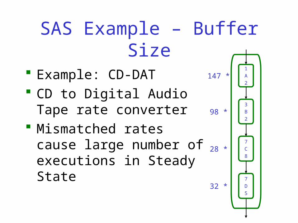
SAS Example – Buffer Size
Example: CD-DAT CD to Digital Audio Tape rate
converter Mismatched rates cause large
number of executions in Steady State
1
A
2
3
B
2
7
C
8
7
D
5
147 *
98 *
28 *
32 *

SAS Example – Buffer Size
Naïve SAS schedule: 147A 98B 28C 32D Required Buffer Size: 714 Unnecessarily large buffer
requirements!
294
196
224
1
A
2
3
B
2
7
C
8
7
D
5
147 *
98 *
28 *
32 *

SAS Example – Buffer Size
Naïve SAS schedule: 147A 98B 28C 32D Required Buffer Size: 714 Unnecessarily large buffer
requirements! Optimal SAS CD-DAT schedule:
49{3A 2B} 4{7C 8D} Required Buffer size: 258
1
A
2
3
B
2
7
C
8
7
D
5

SAS Example – Buffer Size
Naïve SAS schedule: 147A 98B 28C 32D Required Buffer Size: 714 Unnecessarily large buffer
requirements! Optimal SAS CD-DAT schedule:
49{3A 2B} 4{7C 8D} Required Buffer size: 258
1
A
2
3
B
2
7
C
8
7
D
5
6
3 *
2 *

SAS Example – Buffer Size
Naïve SAS schedule: 147A 98B 28C 32D Required Buffer Size: 714 Unnecessarily large buffer
requirements! Optimal SAS CD-DAT schedule:
49{3A 2B} 4{7C 8D} Required Buffer size: 258
1
A
2
3
B
2
7
C
8
7
D
5
6
3 *
2 *

SAS Example – Buffer Size
Naïve SAS schedule: 147A 98B 28C 32D Required Buffer Size: 714 Unnecessarily large buffer
requirements! Optimal SAS CD-DAT schedule:
49{3A 2B} 4{7C 8D} Required Buffer size: 258
1
A
2
3
B
2
7
C
8
7
D
5
49 * 6

SAS Example – Buffer Size
Naïve SAS schedule: 147A 98B 28C 32D Required Buffer Size: 714 Unnecessarily large buffer
requirements! Optimal SAS CD-DAT schedule:
49{3A 2B} 4{7C 8D} Required Buffer size: 258
1
A
2
3
B
2
7
C
8
7
D
5
49 * 6
7 *
8 *
56

SAS Example – Buffer Size
Naïve SAS schedule: 147A 98B 28C 32D Required Buffer Size: 714 Unnecessarily large buffer
requirements! Optimal SAS CD-DAT schedule:
49{3A 2B} 4{7C 8D} Required Buffer size: 258
1
A
2
3
B
2
7
C
8
7
D
5
49 * 6
7 *
8 *
56

SAS Example – Buffer Size
Naïve SAS schedule: 147A 98B 28C 32D Required Buffer Size: 714 Unnecessarily large buffer
requirements! Optimal SAS CD-DAT schedule:
49{3A 2B} 4{7C 8D} Required Buffer size: 258
1
A
2
3
B
2
7
C
8
7
D
5
49 * 6
564 *

SAS Example – Buffer Size
Naïve SAS schedule: 147A 98B 28C 32D Required Buffer Size: 714 Unnecessarily large buffer
requirements! Optimal SAS CD-DAT schedule:
49{3A 2B} 4{7C 8D} Required Buffer size: 258
1
A
2
3
B
2
7
C
8
7
D
5
49 * 6
564 *
196

SAS Example – Buffer Size
Naïve SAS schedule: 147A 98B 28C 32D Required Buffer Size: 714 Unnecessarily large buffer
requirements! Optimal SAS CD-DAT schedule:
49{3A 2B} 4{7C 8D} Required Buffer size: 258
1
A
2
3
B
2
7
C
8
7
D
5
6
56
196

Pull Schedule Example – Buffer Size
Pull Scheduling: Always execute the bottom-most element
possible
CD-DAT schedule: 2A B A B 2A B A B C D … A B C 2D Required Buffer Size: 26 251 entries in the schedule
Hard to implement efficiently, as schedule is VERY large
4
8
14
1
A
2
3
B
2
7
C
8
7
D
5

SAS vs Pull Schedule
Need something in between SAS and Pull Scheduling
Buffer Size Schedule Size
SAS 258 4
Pull Schedule 26 251

Overview
General Stream Concepts StreamIt Details Program Steady State and Initialization Single Appearance and Pull Scheduling Phased Scheduling
Minimal Latency
Results Related Work and Conclusion

Phased Scheduling
Idea: What if we take the naïve SAS schedule, and
divide it into n roughly equal phases? Buffer requirements would reduce roughly
by factor of n Schedule size would increase by factor of n May be OK, because buffer requirements
dominate schedule size anyway!

Phased Scheduling
Try n = 2: Two phases are:
74A 49B 14C 16D 73A 49B 14C 16D
Total Buffer Size: 358 Small schedule increase Greater n for bigger savings
1
A
2
3
B
2
7
C
8
7
D
5
148
98
112

Phased Scheduling
Try n = 3: Three phases are:
48A 32B 9C 10D 53A 35B 10C 11D 46A 31B 9C 11D
Total Buffer Size: 259 Basically matched best SAS result
Best SAS was 258
1
A
2
3
B
2
7
C
8
7
D
5
106
71
82
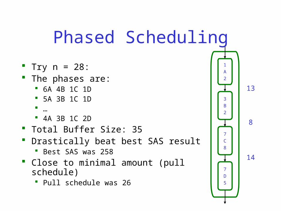
Phased Scheduling
Try n = 28: The phases are:
6A 4B 1C 1D 5A 3B 1C 1D … 4A 3B 1C 2D
Total Buffer Size: 35 Drastically beat best SAS result
Best SAS was 258 Close to minimal amount (pull schedule)
Pull schedule was 26
1
A
2
3
B
2
7
C
8
7
D
5
13
8
14
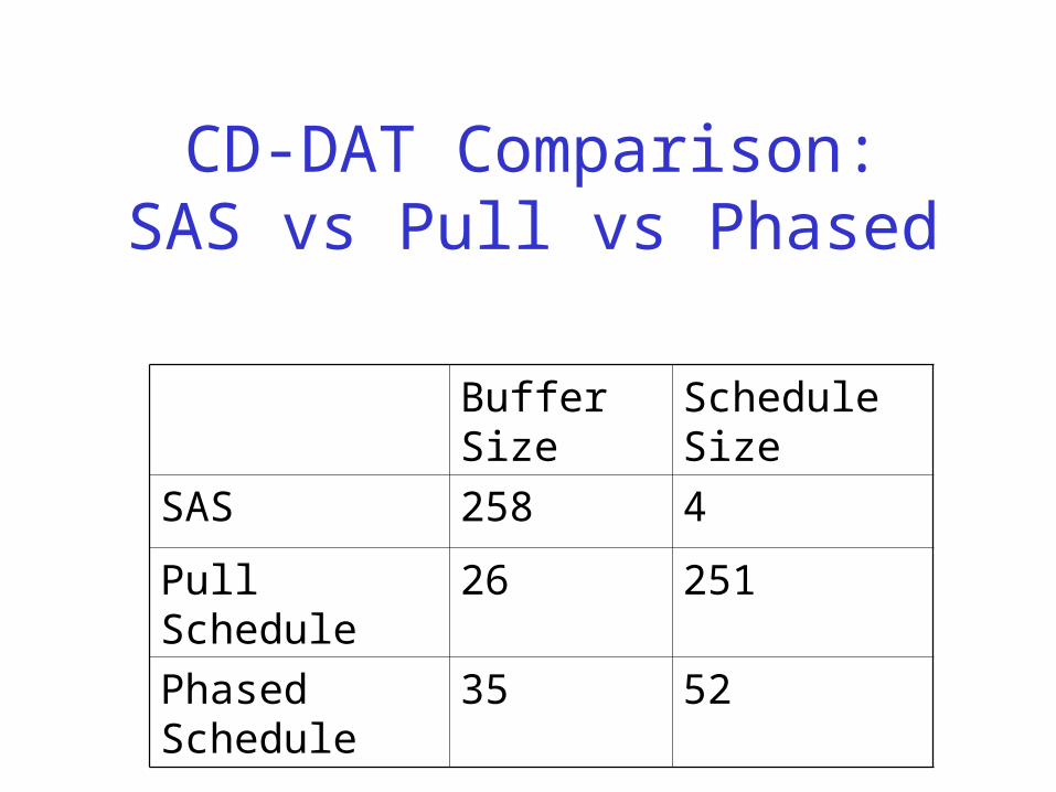
CD-DAT Comparison:SAS vs Pull vs Phased
Buffer Size Schedule Size
SAS 258 4
Pull Schedule 26 251
Phased Schedule 35 52

Phased Scheduling
Apply technique hierarchically Children have several phases
which all have to be executed Automatically supports cyclo-
static filters Children pop/push less data, so
can manage parent’s buffer sizes more efficiently
CD-DAT
CD reader
DAT
recorder
Equalizer

Phased Scheduling
What if a Steady State of a component of a FeedbackLoop required more data than available?
Single Appearance couldn’t do separate compilation!
Phased Scheduling can provide a fine-grained schedule, which will always allow separate compilation (if possible at all)

Overview
General Stream Concepts StreamIt Details Program Steady State and Initialization Single Appearance and Pull Scheduling Phased Scheduling
Minimal Latency
Results Related Work and Conclusion

Minimal Latency Schedule
Every Phase consumes as few items as possible to produce at least one data item
Every Phase produces as many data items as possible
Guarantees any schedulable program will be scheduled without deadlock
Allows for separate compilation For details, see our paper

Minimal Latency Scheduling
Simple FeedbackLoop with a tight delay constraint
Not possible to schedule using SAS
Can schedule using Phased Scheduling Use Minimal Latency
Scheduling
3
B
5
4
L
4
2
1 1
1 5
6
delay = 10
*4
*8
*20
*5

Minimal Latency Scheduling
Minimal Latency Phased Schedule:
3
B
5
4
L
4
2
1 1
1 5
6
delay = 10
10
0
0
0

Minimal Latency Scheduling
Minimal Latency Phased Schedule: join 2B 5split L
3
B
5
4
L
4
2
1 1
1 5
6
delay = 10
9
1
0
0

Minimal Latency Scheduling
Minimal Latency Phased Schedule: join 2B 5split L join 2B 5split L 3
B
5
4
L
4
2
1 1
1 5
6
delay = 10
8
2
0
0

Minimal Latency Scheduling
Minimal Latency Phased Schedule: join 2B 5split L join 2B 5split L join 2B 5split L
3
B
5
4
L
4
2
1 1
1 5
6
delay = 10
7
3
0
0

Minimal Latency Scheduling
Minimal Latency Phased Schedule: join 2B 5split L join 2B 5split L join 2B 5split L join 2B 5split 2L
3
B
5
4
L
4
2
1 1
1 5
6
delay = 10
10
0
0
0

Minimal Latency Schedule
Minimal Latency Phased Schedule: join 2B 5split L join 2B 5split L join 2B 5split L join 2B 5split 2L
Can also be expressed as: 3 {join 2B 5split L} join 2B 5split 2L
Common to have repeated Phases
3
B
5
4
L
4
2
1 1
1 5
6
delay = 10

Why not SAS?
Naïve SAS schedule 4join 8B 20split 5L: Not valid because 4join
consumes 20 data items Would like to form a loop-nest
that includes join and L But multiplicity of executions
of L and join have no common divisors
3
B
5
4
L
4
2
1 1
1 5
6
delay = 10
*4
*8
*20
*5

Overview
General Stream Concepts StreamIt Details Program Steady State and Initialization Single Appearance and Pull Scheduling Phased Scheduling
Minimal Latency
Results Related Work and Conclusion
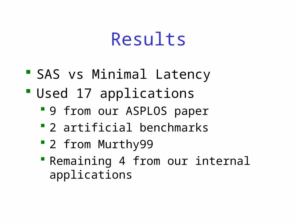
Results
SAS vs Minimal Latency Used 17 applications
9 from our ASPLOS paper 2 artificial benchmarks 2 from Murthy99 Remaining 4 from our internal applications

Results - Buffer Size
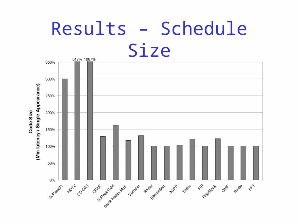
Results – Schedule Size

Results - Combined

Overview
General Stream Concepts StreamIt Details Program Steady State and Initialization Single Appearance and Pull Scheduling Phased Scheduling
Minimal Latency
Results Related Work and Conclusion

Related Work
Synchronous Data Flow (SDF) Ptolemy [Lee et al.] Many results for SAS on SDF
Memory Efficient Scheduling [Bhattacharyya97] Buffer Merging [Murthy99]
Cyclo-Static [Bilsen96] Peeking in US Navy Processing Graph Method
[Goddard2000] Languages: LUSTRE, Esterel, Signal

Conclusion
Presented Phased Scheduling Algorithm Provides efficient interface for hierarchical scheduling Enables separate compilation with safety from deadlock Provides flexible buffer / schedule size trade-off Reduces latency of data throughput
Step towards a large scale hierarchical stream programming model
Phased Schedulingof Stream Programs
StreamIt Homepage
http://cag.lcs.mit.edu/streamit


![streamit-language-lecture - for pdf [Read-Only] · 2009. 3. 3. · Architectures (ASPLOS 02) Phased Scheduling (LCTES 03) Cache Aware Optimization (LCTES 05) Load-Balanced Rendering](https://static.documents.pub/doc/80x56/5fe4dc06dc61e22ba315e8c7/streamit-language-lecture-for-pdf-read-only-2009-3-3-architectures-asplos.jpg)


