An analysis of coherent optical FMCW is presented. Itshows the limitations imposed on measurements ofdiscrete reflections and of Rayleigh backscattering dueto phase noise originating in the finite coherence lengthof the optical source. The dependence of the range foraccurate measurements on particular parameters of theoptical system is discussed in the general case and forthree specific laser sources.
Optical time domain reflectometry is a well-established tool for the non-destructive characterization of fiberoptic networks [1]. This characterization may be for the purpose ofmonitoring long or short haul communication networks, or for more specialized sensing applications. In the latter case, an external parameter affects the propagation of light throughthe network. For example, it might change the reflection at specific sensing sites, or changethe polarization state in a continuously distributed fashion [2]. In general, the ideal reflectometry system would have a spatial resolution high enough to locate closely separated sitesof reflection within the network under test, at interfaces in connectors, for example. In addition, the sensitivity would be high enough to measure Rayleigh backscattering throughoutthe fiber network. The level of backscattering, its rate of change with distance, and thelocations and sizes of any discontinuities, comprise useful information on distributed andlocalized losses, in the fiber and at splices or connectors.
In time domain reflectometry techniques, in which systems are probed with pulses of radiation, spatial resolution is improved as the pulses are made shorter, and the measurementbandwidth is increased. This raises the noise levels detected, and so reduces the dynamicrange ofthe measurements. The dynamic range of frequency domain systems, however, whichuse continuous wave probes, is independent of spatial resolution. This basic feature givestechniques like frequency-modulated continuous wave ranging (FMCW) [3] the potential toachieve high spatial resolution without sacrificing dynamic range. Applying this to coherentoptical reflectometry [4] gains the additional advantage of the high sensitivity characteristicof coherent optical detection.
A critical feature in a coherent optical FMCW system is the source, which can determine theachievable spatial resolution and range. High spatial resolution in the measurement dependson the source having a large, phase-continuous, linear tuning range. The extent to whichthe source departs from perfect coherence, and so produces phase noise in the output signalspectrum, limits two aspects of system performance. One is the distance over which measurements of discrete reflections can be made, before incoherent mixing predominates, andthe other is the dynamic range between the reflection signal of interest and the level of phasenoise. The requirements on the source coherence length relative to measurement range, andthe significance of such aspects as the measurement bandwidth and the reflection strengthhave not been expressed with clarity and precision. Although some initial experimental workhas been reported [5, 6, 7], there remains a need for a more complete theoretical foundationto these aspects of coherent FMCW reflectometry.
In this paper, we present an outline of a quantitative analysis of a model of coherent FMCWreflectometry which considers the phase noise due to finite laser linewidth. We discuss howthe results of this analysis impact the measurement ranges for discrete reflections and forRayleigh backscattering in the presence of such reflections.
2 Theory
The basis of coherent FMCW reflectometry [3] is the interferometric mixing of two signalsoriginating from the same linearly chirped source, one signal following a "test" path, whilethe other follows a reference path. Any time delays between the signals reflected backfrom sites along the test path and the signal from the reference reflection give rise to beat
. frequencies in the mixed output. The values of the beat frequencies are proportional to
1
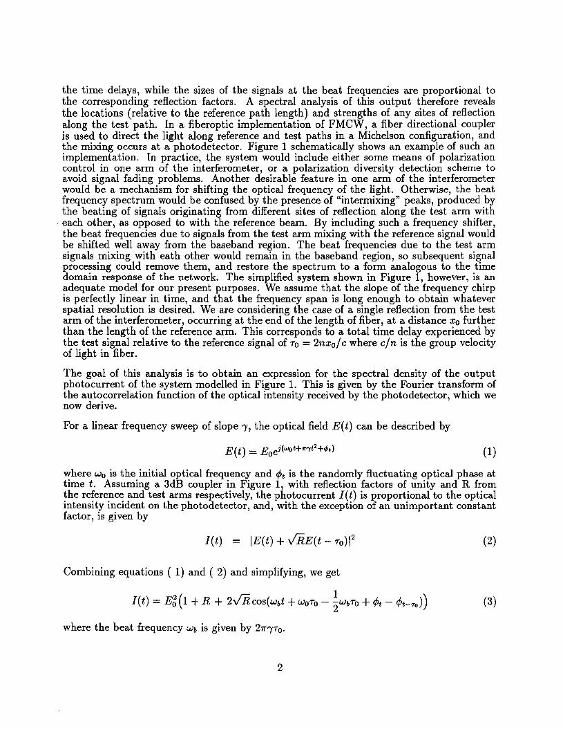
the time delays, while the sizes of the signals at the beat frequencies are proportional tothe corresponding reflection factors. A spectral analysis of this output therefore revealsthe locations (relative to the reference path length) and strengths of any sites of reflectionalong the test path. In a fiberoptic implementation of FMCW, a fiber directional coupleris used to direct the light along reference and test paths in a Michelson configuration, andthe mixing occurs at a photodetector. Figure 1 schematically shows an example of such animplementation. In practice, the system would include either some means of polarizationcontrol in one arm of the interferometer, or a polarization diversity detection scheme toavoid signal fading problems. Another desirable feature in one arm of the interferometerwould be a mechanism for shifting the optical frequency of the light. Otherwise, the beatfrequency spectrum would be confused by the presence of "intermixing" peaks, produced bythe beating of signals originating from different sites of reflection along the test arm witheach other, as opposed to with the reference beam. By including such a frequency shifter,the beat frequencies due to signals from the test arm mixing with the reference signal wouldbe shifted well away from the baseband region. The beat frequencies due to the test armsignals mixing with eath other would remain in the baseband region, so subsequent signalprocessing could remove them, and restore the spectrum to a form analogous to the timedomain response of the network. The simplified system shown in Figure 1, however, is anadequate model for our present purposes. We assume that the slope of the frequency chirpis perfectly linear in time, and that the frequency span is long enough to obtain whateverspatial resolution is desired. We are considering the case of a single reflection from the testarm of the interferometer, occurring at the end of the length of fiber, at a distance Xo furtherthan the length of the reference arm. This corresponds to a total time delay experienced bythe test signal relative to the reference signal of TO = 2nxo/c where cln is the group velocityof light in fiber.
The goal of this analysis is to obtain an expression for the spectral density of the outputphotocurrent of the system modelled in Figure 1. This is given by the Fourier transform ofthe autocorrelation function of the optical intensity received by the photodetector, which wenow derive.
For a linear frequency sweep of slope " the optical field E(t) can be described by
E(t) = Eoei (wot+1r"(t2 +tPt} (1)
where Wo is the initial optical frequency and 4>t is the randomly fluctuating optical phase attime t. Assuming a 3dB coupler in Figure 1, with reflection factors of unity and R fromthe reference and test arms respectively, the photocurrent I(t) is proportional to the opticalintensity incident on the photodetector, and, with the exception of an unimportant constantfactor, is given by
I(t) = IE(t) + .JRE(t - To)l2
Combining equations ( 1) and ( 2) and simplifying, we get
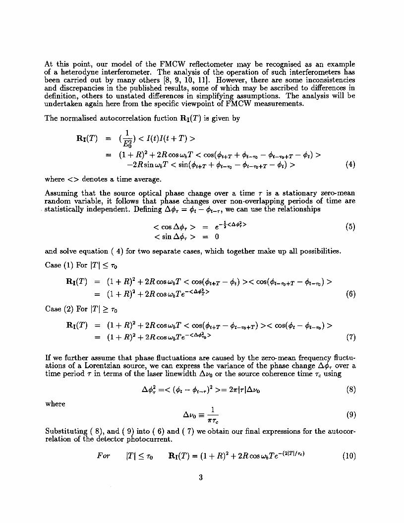
At this point, our model of the FMCW reflectometer may be recognised as an exampleof a heterodyne interferometer. The analysis of the operation of such interferometers hasbeen carried out by many others [8, 9, 10, 11]. However, there are some inconsistenciesand discrepancies in the published results, some of which may be ascribed to differences indefinition, others to unstated differences in simplifying assumptions. The analysis will beundertaken again here from the specific viewpoint of FMCW measurements.
The normalised autocorrelation fuction RI(T) is given by
Assuming that the source optical phase change over a time T is a stationary zero-meanrandom variable, it follows that phase changes over non-overlapping periods of time are
. statistically independent. Defining tl¢>r = ¢>t - ¢>t-r, we can use the relationships
< cos tl¢>r > = e- t<A4>; >
< sin tl¢>r > = 0
and solve equation ( 4) for two separate cases, which together make up all possibilities.
If we further assume that phase fluctuations are caused by the zero-mean frequency fluctuations of a Lorentzian source, we can express the variance of the phase change tl¢>r over atime period T in terms of the laser linewidth tlvo or the source coherence time Tc using
where
(8)
(9)
Substituting ( 8), and ( 9) into ( 6) and ( 7) we obtain our final expressions for the autocorrelation of the detector photocurrent.
For ITI ::; TO
3
(10)
For (11)
Figure 2 is a plot of the autocorrelation function described by equations ( 10) and ( 11),clearly showing the transition at the interferometer delay time from an exponentially decaying sinusoid to one with constant amplitude. A qualitative understanding of the system'sbehaviour may be gained from considering how different system parameters would changethe shape of this plot, and so the corresponding spectral density.
For the case of complete incoherence, corresponding to an infinitely long interferometerdelay, the exponentially decaying envelope never reaches a transition point. Its Fouriertransform (neglecting the DC component) would therefore be a Lorentzian, centred on thebeat frequency Wb' This matches our expectations for the interferometric output from anincoherent source, as found in delayed self-heterodyne measurements. For the oppositeextreme of perfect coherence, or zero interferometer delay, the autocorrelation plot wouldjust be a sinusoid of constant amplitude, and its Fourier transform would be a delta functionat the beat frequency.
To obtain a general expression for the two-sided spectral density of the photocurrent, SI(J),we take the Fourier transform of the autocorrelation function. Beginning with
SI(J) L: RI(T)e-(21ri/T)dT
- i: [(1 + R)2 +2RcoswbTe-(2ITI/'Tc)]e-(21ri/T)dT
+1000
[(1+ R)2 +2RcoswbTe-(27b!'Tc)]e-(21ri/T)dT
+i:o[(1 +R? +2R cos WbT e-(27lJ!'Tc)] e-(21ri/T)dT (12)
and working through the algebraic manipulations we finally obtain
where Ib = Wb/21r. A more useful expression to relate to experimental measurements is theone-sided spectral density S}l) (J) given by
Three terms make up the spectral density function. The first is a delta function at DC, whichcorresponds to the average level of optical power reaching the photodetector, dependent onthe value of the reflection factor R. The second is a delta function at the beat frequency,weighted by a factor including R and an exponential function of the ratio of delay to coherencetime. This second term corresponds to the FMCW beat signal arising directly from the
4
reflection site, reduced in magnitude by the system's degree of incoherence. The third termis a continuous function of frequency, strongly affected by the coherence time and the delaytime. It represents the distribution of phase noise around the beat frequency. Equation ( 14)can be used to generate plots to show how the distribution of phase noise, the last term inthe expression, evolves as a function of system coherence, from a Lorentzian of halfwidthequal to twice the laser linewidth for a low coherence system, to a sinc2 function with 'zeros'at intervals of the reciprocal of the delay time, for a high coherence system [10].
So far in the analysis, we have ignored the phenomenon of Rayleigh backscattering, whichwould effectively contribute a continuum of small 'reflections' from the fiber in the test arm,up to the distance xo. After coherent mixing with the reflection from the reference arm,the resulting photocurrent would have a spectral density function whose magnitude can becalculated as follows.
If we take S to be the backscattering capture coefficient and as to be the loss coefficientdue to Rayleigh backscattering [12], the fraction RRBS of the incident power scattered into aguided wave travelling in the backward direction is given by
RRBS = Sas~x (15)
where ~x is the system's spatial resolution. In an FMCW system, the spatial resolution isgiven by
c c~x = - = -~f (16)
2nFs 2n')'
where F, is the optical frequency span swept through during the measurement time, andthe effective measurement time is equal to the reciprocal of the frequency resolution of themeasurement, ~f, hereafter called the measurement bandwidth.
From ( 15) and ( 16), the one-sided spectral density S}l)(f) due to Rayleigh backseat-RBS
tering, normalised with respect to the input power, can be expressed as
S}l)(f)I = Sasi-RBS n')'
(17)
Other contributions to the detected spectral density include relative intensity noise from the. source, and shot noise at the receiver. These are strongly system-specific, and may warrantattention if they dominate phase noise or the Rayleigh backscattering level in a particularapplication.
From the viewpoint of FMCW reflectometry, cases of high coherence are most relevant,and an approximation of equation ( 14) for high coherence would be valuable. An analyticalderivation of such an approximation can be carried out more easily by returning to equations( 10) and ( 11). The assumption of high coherence is expressed quantitatively by settingTolTe « 1. Equations ( 10) and ( 11) then simplify to
For
For
ITI < TO
ITI > TO
4RITIRI(T) RJ (1 + R)2 + 2R cosWbT - -- coswbTTe
RI(T) RJ (1 +R)2 +2R cosWbT
5
(18)
The autocorrelation amplitude decays linearly rather than exponentially in this high coherence case, before reaching a constant value. 81(1), the two-sided spectral density ofthe corresponding photocurrent, is given by the Fourier transform of the autocorrelationfunction.
81(1) ~ 1:[(1 + R? + 2Rcos27r!bT]e-(21rijT)dT
_j1"() [4RITI] cos 27r!bT e-(21rj jT)dT-'To Tc
which leads to the following expression for the one-sided spectral density
(19)
This describes a delta function at DC, a delta function at the beat frequency, and a sinc2
function, with zeros at the reciprocal of the delay time, centred at the beat frequency.
Figure 3 shows a typical plot of the spectral density of the detected photocurrent, takenfrom equations ( 20) and ( 17) in combination. The backscattering contribution stops atthe beat frequency of the main reflection, as we have assumed the reflection occurs at theend of the fiber. Notice the sinc2 rippling of the phase noise, gradually falling below thelevel of the Rayleigh backscattering on the low frequency (fiber) side of the reflection signalpeak. It is clear that the dynamic range of the measurement may be significantly reducedclose to the reflection peak because of the phase noise. Expressions are given in the figurefor the average level of Rayleigh backscattering, the peak value of phase noise, and the deltafunction weights at DC and the beat frequency.
In a real measurement, the power in a given bandwidth is measured rather than spectraldensity, and the phase noise power, any other noise power such as RIN, and the Rayleighbackscattering power would be proportional to the bandwidth of the measurement system.The DC and beat frequency signals, however, would be of finite but fixed heights, independent of bandwidth. This means that if we could improve the spatial resolution by increasingthe source's frequency span, and increase the measurement time by the same factor, to keepthe slope I constant, the corresponding reduction in the measurement bandwidth wouldcause all noise and backscattering levels to be lowered by exactly the same amount. Wewould therefore not suffer any reduction in the dynamic range of the measurement. Thisproportionality between spatial resolution and measurement bandwidth is one of the mainadvantages of FMCW over time domain reflectometry. In the latter technique, an improvement in spatial resolution occurs at the cost of an increase in the measurement bandwidth,
.which both lowers the backscattering signal and raises the noise levels, and so greatly reducesthe dynamic range of the measurement.
3 Application
The importance of equations ( 14) and ( 17) to coherent FMCW reflectometry lies in the possibility they offer of predicting measurement performance for various combinations of systemparameters. This may be useful in designing a system to fit a particular measurement need,or in defining the measurement capabilities of a given system. As an example of the latter
6
situation, suppose for a given source of known wavelength, linewidth, and phase-continuoustuning range, we wish to know how far down a fiber network a Rayleigh backscattering signal is detectable in the presence of a reflection of some known magnitude at the fiber end.Choosing a practical sweep rate, and corresponding measurement bandwidth, the phase noiseterm of equation ( 14) could be employed to determine, for the given parameters, the peakvalue of phase noise power, relative to the input power, as a function of the fiber length.
The curve labelled 'phase noise' in Figure 4 shows the result of following the procedure justdescribed, for a specific case. The qualitative features of this curve and the others in thisfigure are, however, true for the general case, with only the details and the relative positionsof the curves changing for specific system parameter changes. The phase noise curve shownfollows the pattern of all such curves - a linear increase with distance, until the onset ofincoherent behaviour, where it flattens out. The curve labelled 'reflection peak' representsthe signal power due to the discrete reflection, obtained from the second term in equation( 14), which is determined by the source linewidth and the reflection factor. Notice that thesignal drops very slowly with distance over the coherent measurement range, and then fallsvery sharply, as the light reflected back from the test arm becomes incoherent with the lightreflected back from the reference arm. As an indication of the onset of incoherennt mixing,we could arbitrarily choose the point at which the power of the beat frequency signal fallsby 1dB from its value at perfect coherence, or zero path delay. We could then propose thatthis system should not be used to make reflection strength measurements beyond this point,marked 'a' in the figure, which is determined by the source linewidth, and is independent ofthe reflection factor, R. The curve labelled 'Rayleigh backscattering' shows the average levelof the Rayleigh backscattered power, obtained by multiplying the expression in in equation( 17) by the resolution bandwidth. at the wavelength of interest in equation ( 17) andmultiplying by the resolution bandwidth. To answer our main question on the Rayleighbackscattering measurement range, we can see that up to the fiber distance marked 'b' inFigure 4, the level of Rayleigh backscattering is above the phase noise. For longer fibers,
. the phase noise from the end reflection will dominate the backscattering signal. However, inorder to make Rayleigh backscattering measurements in fibers shorter than 'b', it would beessential to keep any other noise sources, such as shot noise or the optical source's relativeintensity noise (RIN), below the level of the backscattering signal.
It should be noted that for a fixed value of the frequency slope, the crossover point 'b' isindependent of the spatial resolution, since the phase noise and the Rayleigh backscatteringsignals have the same dependence on measurement bandwidth. However, if we were to reduce the slope, and the measurement bandwidth by the same factor, so keeping the spatialresolution constant, the backscattering level would be unchanged but the phase noise curvewould decrease, resulting in an increase om the measurement range for Rayleigh backseattering.
The curves in Figure 4 show the various signal strengths plotted against distance for givensource parameters. An alternative set of curves could be obtained by plotting the powers dueto phase noise, Rayleigh backscattering, and the reflection signal itself as functions of laserlinewidth for a fixed value of measurement path delay. This could help in making a decisionon a suitable source for an FMCW measurement system for a specific application. Figure5 shows a typical set of such curves, generated from equations ( 14) and ( 17), following asimilar procedure to that for Figure 4. The significance of the point marked 'aa' in this figureis the same as that of 'a' in Figure 4, showing the 1dB limit for coherent measurements, nowin terms of the allowable linewidth for the desired measurement range. In the same way,point 'bb' marks the limit for Rayleigh backscattering measurements in terms of the allowable
7
linewidth for a source of given tuning range, tuning rate, and measurement bandwidth, inthe presence of an end reflection.
Let us take some specific cases of practical sources likely to be of some interest in FMCWreflectometry. Consider first an external cavity laser of 100 KHz linewidth, operating at 1.3utu, and tunable through a span of 100 GHz without mode hops. We might be interested infinding out how far down a fiber network we would be able to detect a Rayleigh backscatteringsignal in the presence of a 4 % Fresnel reflection at the fiber end. In order to take fulladvantage of the 100 GHz frequency span, and obtain the corresponding spatial resolutionof Imm, we could choose a sweep rate I of 1013 Hz/s, and collect data during a time intervalof 10 IDS. This would mean a measurement bandwidth of 100 Hz. The other numbers weneed are the coherence time corresponding to the linewidth of 100 KHz, which is 3.18 ps,the reflection factor R, which we set at 0.04, and the appropriate values of scattering factorand attenuation due to scattering. For standard single mode fiber, we take Os = 0.001 andS = 8.1xl0-s per meter [1]. Following the procedure described above, to generate curves ofpower against fiber length, we obtain a value for the transition point 'a', marking the rangefor coherent reflectometry, as '" 100 m, and a value for 'b' of '" 30 cm, indicating that phasenoise arising from the 4% end reflection would dominate Rayleigh backscattering in fiberlengths any longer than this.
If we were to reduce the slope I and the measurement bandwidth by a factor of 10, to1012 Hz/s and 10 Hz respectively, the spatial resolution would be unchanged, at Irnm, thebackscattering level would remain in place, but the phase noise curve would shift down by10 dB, moving the point 'b' to about 3 m - a tenfold increase in the measurement range.
Now consider a Nd:YAG ring laser source, at 1.32 pm, with a linewidth of 100 Hz, anda phase-continuous tuning range of 10 GHz. The best spatial resolution possible wth thistuning range is 1 em, and could be achieved by choosing a sweep rate of 1011 Hz/ s and abandwidth of 10 Hz. We find that the points 'a' and 'b' occur at about 50 Km and 100 mrespectively. These improvements in measurement range compared to the external cavitylaser might be important enough in some applications to outweigh the disadvantage of thepoorer resolution. Other features, such as reliability or ease of operation, may also deserveserious consideration in the process of making a choice between the two types of source for
. a particular system.
Finally, consider a semiconductor source, a 1.55 pm distributed feedback laser of 25 MHzlinewidth and a maximum phase-continuous tuning range of 500 GHz. We could keep themeasurement bandwidth at 10 Hz, and choose a sweep rate of 5xl012 Hz/s, to make use of thefull tuning range, and obtain a spatial resolution of 0.2 mm. Estimating the attenuation dueto scattering at 1.55 pm by assuming an inverse fourth power relationship with wavelength[1], we obtain Os = 4xl0-s per m. Plotting the power curves against fiber length as before, wewould find that the useful measurement range for discrete reflections was about 50 em, andthat the range for Rayleigh backscattering measurements in the presence of a 4 % reflectionwas about 2 cm. So, although the spatial resolution would be very good, due to the largetuning range, the measurement ranges would be quite short, due to the short coherencelength of this type of source.
8
4 Conclusion
The presence of phase noise in the spectrum of the signal output from a coherent optical FMCW reflectometry system limits the ranges over which either discrete reflections orRayleigh backscattering may be accurately measured. System parameters that determinethese limits include the linewidth of the source, the measurement bandwidth, the frequencychirp rate, and the scattering characteristics of the fiber. The general expressions derivedfor FMCW measurement systems have been used to calculate the limits for three sources ofpractical interest.
The first case was a 1.3 JLm source of 100 KHz linewidth, phase-continuously tunable through100 GHz. These numbers would be quite feasible for an external cavity laser. A system basedon such a source was shown to have a useful range for discrete reflection measurement oftv 100 m. Its range for Rayleigh backscattering measurements in the presence of a 4 %reflection, with a spatial resolution of 1mm, and a measurement time of lOOms, was 3 m.The second case was a 1.32 JLm source of 100 Hz linewidth and a phase-continuous tuningrange of 10 GHz. These numbers could well describe a Nd:YAG ring laser. The correspondingFMCW system was shown to have ranges of tv 50 Km and 100 m for discrete reflection andRayleigh backscattering measurements respectively, with a spatial resolution of 1 em and ameasurement time of 100 ms. The third case was a 1.55 JLm source of 25 MHz linewidth,and a phase-continuous tuning range of 500 GHz. Distributed feedback lasers can havesuch characteristics. Measurement ranges in this case were tv 50 em for discrete reflectionsand tv 2 em for Rayleigh backscattering levels, with a spatial resolution of 0.2 mm, for ameasurement time of 100 IDS and phase noise due to a 4 % reflection.
5 References[1] Healey, P.: "Instrumentation principles for optical time domain reflectometry" , J. Phys.
E: Sci. Instrum. 1986, 19, pp. 334-341.
[2] Rogers, A. J.: "Polarization optical time domain reflectometry", Electronics Letters,1980, 16, pp. 489-490.
[3] Hymans, A. J., and Lait, J.: "Analysis of a Frequency Modulated Continuous WaveRanging System", Proc. lEE, 1960, l07B, pp. 365-372.
[4] Uttam, D., and Culshaw, B.: "Precision Time Domain Reflectometry in OpticalFiber Systems Using a Frequency Modulated Continuous Wave Ranging Technique",IEEE/OSA J. Lightwave Technology, 1985, LT-3, pp. 971-977.
[5] Sorin, W. V., Donald, D. K., Newton, S. A., and Nazarathy, M.: "Coherent FMCWReflectometry Using a Temperature Tuned Nd:YAG Ring Laser", IEEE Photonics Technology Letters, 1990, 2, pp. 902-904.
[6] Brinkmeyer, E., and Glombitza, U.: "High-resolution coherent frequency-domain reflectometry using continuously tuned laser diodes", Technical Digest, OFC'91, 1991, paperWN2, p. 129.
[7] Venkatesh, S., Sorin, W. V., Donald, D. K., and Heffner, B. L.: "Coherent FMCWreflectometry using a piezoelectrically tuned Nd:YAG ring laser", submitted to OFS 8,1991.
9
[8] Armstrong, J. A.: "Theory of interferometric analysis of laser phase noise", J. O. S.A., 1966, 56, pp. 1024-1031.
[9] Gallion, P. B., and Debarge, G.: "Quantum phase noise and field correlation in singlefrequency semiconductor laser systems", IEEE J. Q. E. , 1984, QE-20, pp. 343-349.
. [10] Richter, L. E., Mandelberg, H. I., Kruger, M. S., and McGrath, P. A.: "Linewidth determination from self-heterodyne measurements with subcoherence delay times", IEEEJ. Q. E. , 1986, QE-22, pp. 2070-2074.
[11] Okoshi, T., and Kikuchi. K.:"Coherent Optical Fiber Communications", published byKTK Scientific Publishers/Tokyo, 1988, pp. 86-90.
[12] Brinkmeyer, E,:"Analysis of the backscattering method for single-mode optical fibers",J. O. S. A. , 1980, 70, pp. 1010-1012.
Figures
Figure 1. Fiberoptic implementation of coherent FMCW reflectometry, showing chirpedlaser source, reference and test arms of interferometer with corresponding optical fields, andthe detector photocurrent.
Figure 2. Autocorrelation RI(T) of the photocurrent I(t).
Figure 3. One sided spectral density S}l)(J) of the photocurrent I(t) for a high coherencesystem, showing the delta functions at DC and the beat frequency, and the distribution ofphase noise around the beat frequency, with the average level of Rayleigh backscatteringsuperimposed on the low frequency side.
Figure 4. Phase noise power, Rayleigh backscattering power, and end-reflection power asfunctions of fiber length.
Figure 5. Phase noise power, Rayleigh backscattering power, and end-reflection power asfunctions of source linewidth.