Phases, phase equilibria, and phase rules in low-dimensional systemsT. Frolov and Y. Mishin Citation: The Journal of Chemical Physics 143, 044706 (2015); doi: 10.1063/1.4927414 View online: http://dx.doi.org/10.1063/1.4927414 View Table of Contents: http://scitation.aip.org/content/aip/journal/jcp/143/4?ver=pdfcov Published by the AIP Publishing Articles you may be interested in Simplified Onsager theory for isotropic–nematic phase equilibria of length polydisperse hard rods J. Chem. Phys. 117, 5421 (2002); 10.1063/1.1499718 Perturbative polydispersity: Phase equilibria of near-monodisperse systems J. Chem. Phys. 114, 1915 (2001); 10.1063/1.1333023 Phase equilibria and thermodynamic properties of hard core Yukawa fluids of variable range from simulationsand an analytical theory J. Chem. Phys. 112, 10358 (2000); 10.1063/1.481673 Phase equilibria in binary polymer blends: Integral equation approach J. Chem. Phys. 109, 10042 (1998); 10.1063/1.477673 Calculation of solid-fluid phase equilibria for systems of chain molecules J. Chem. Phys. 109, 318 (1998); 10.1063/1.476566

This article is copyrighted as indicated in the article. Reuse of AIP content is subject to the terms at: http://scitation.aip.org/termsconditions. Downloaded to IP:

129.6.153.96 On: Tue, 28 Jul 2015 15:17:55

THE JOURNAL OF CHEMICAL PHYSICS 143, 044706 (2015)

Phases, phase equilibria, and phase rules in low-dimensional systemsT. Frolov1,a) and Y. Mishin2,b)1Department of Materials Science and Engineering, University of California, Berkeley, California 94720, USA2Department of Physics and Astronomy, MSN 3F3, George Mason University, Fairfax, Virginia 22030, USA

(Received 7 May 2015; accepted 15 July 2015; published online 28 July 2015)

We present a unified approach to thermodynamic description of one, two, and three dimensionalphases and phase transformations among them. The approach is based on a rigorous definitionof a phase applicable to thermodynamic systems of any dimensionality. Within this approach, thesame thermodynamic formalism can be applied for the description of phase transformations in bulksystems, interfaces, and line defects separating interface phases. For both lines and interfaces, werigorously derive an adsorption equation, the phase coexistence equations, and other thermodynamicrelations expressed in terms of generalized line and interface excess quantities. As a generalizationof the Gibbs phase rule for bulk phases, we derive phase rules for lines and interfaces and predict themaximum number of phases than may coexist in systems of the respective dimensionality. C 2015 AIPPublishing LLC. [http://dx.doi.org/10.1063/1.4927414]

I. INTRODUCTION

Surfaces and interfaces can affect many properties ofmaterials ranging from chemical reactivity to wetting, mechan-ical behavior, and thermal and electric resistance.1 It has longbeen known that interface properties can suddenly changedue to an abrupt change in their atomic structure and/or localchemical composition. Such changes are often interpreted astransformations between different interface phases and areusually described by well-established thermodynamic theoriesof phase transformations. Despite many years of experimentaland theoretical studies, certain thermodynamic aspects ofinterface phases and interface phase transformations remainunclear. In fact, there is even a controversy about the ther-modynamic nature of interface phases, namely, whether theyshould be treated as a particular case of the general conceptof a phase in thermodynamics, or as something fundamentallydifferent from bulk phases. As a consequence, terminologicaldisagreements arose in the materials community, with someauthors referring to interface phases as “phases”2–12 whileothers prefer the new term “complexion”13–18 introduced toavoid the association with bulk phases.

The goal of this paper is to examine the parallel betweenphase transformations in bulk and low-dimensional systemsfrom the standpoint of classical thermodynamics. Some ofthe questions that we seek to answer include the following:To what extent can one apply the formalism and termi-nology of classical three-dimensional (3D) thermodynamicsto describe two-dimensional (2D) phases at interfaces and one-dimensional (1D) phases within line defects? Is it justifiableto treat transformations between 2D and 1D phases the sameway as we treat transformations between bulk (3D) phases?

To answer these questions, we start by reviewing theoriginal definition of a phase,19 the modern definitions,20,21 and

a)Electronic address: timfrol@berkeley.edub)Electronic address: ymishin@gmu.edu

their applicability low-dimensional thermodynamic systems.We then formulate a unified definition of a phase that spansall dimensionalities. This definition identifies the conceptof a phase with a fundamental equation of state possessinga particular set of mathematical properties. This unifieddefinition leads to a unified treatment of phase equilibriaamong phases of different dimensionality. Applying thisunified thermodynamic formalism, we rigorously derive 2Dand 1D versions of the adsorption equation, both expressedin terms of generalized interface (respectively, line) excesses.We also derive generalized Clapeyron-Clausius type equationsdescribing the hypersurfaces of thermodynamic equilibriumbetween bulk, interface, or line phases, as well as generalizedphase rules for interfaces and line defects.

The approach applied in this work is largely influenced bythe attempts of many authors to formulate the logical structureof thermodynamics in the form of axioms and postulates in amanner similar to mathematical theories.20–29 It is not our goalto pursue a complete axiomatic structure of thermodynamicsin the present paper. However, the formulation of certainkey points in the form of definitions and postulates helpsus emphasize important concepts, logical connections, andassumptions that are often implied but not stated explicitly,or simply overlooked. The fundamental equations of stateare formulated for simple isotropic systems such as multi-component fluids. While extensions to other systems arepossible in the future, in this paper, we wish to focus theattention on the most basic concepts and not be distracted bytechnical difficulties that arise in addressing more complexsystems.

As already mentioned, the approach proposed hereis restricted to classical thermodynamics. Thus, statistical-mechanical treatments of phases of any dimensionality arebeyond the scope of this paper. The interested reader isreferred to special literature in the respective fields, such asthe Rawlinson and Widom book30 on molecular-level theoriesof interfaces. Likewise, we refrain from making any model

0021-9606/2015/143(4)/044706/14/$30.00 143, 044706-1 © 2015 AIP Publishing LLC

This article is copyrighted as indicated in the article. Reuse of AIP content is subject to the terms at: http://scitation.aip.org/termsconditions. Downloaded to IP:

129.6.153.96 On: Tue, 28 Jul 2015 15:17:55

044706-2 T. Frolov and Y. Mishin J. Chem. Phys. 143, 044706 (2015)

assumptions regarding the local behavior of properties insidelow-dimensional phases. In particular, despite the success ofinterface theories based on gradient thermodynamics,31,32 theyare not part of the present discussion. Instead, we adhere to thepurely thermodynamic approach in which low-dimensionalphases are treated in terms of interface or line excess quantitieswithout attempting to characterize the excess regions in a moredetailed (but necessarily approximate) manner.

II. PHASES IN BULK THERMODYNAMICS

A. Definition of a phase

The term “phase” was introduced by Gibbs,19 who definedphases rather vaguely as “different homogeneous bodies” that“differ in composition or state” (Ref. 19, p. 96). Despite thevagueness of this verbal definition, the equations written byGibbs make it clear that by a phase, Gibbs understood acontinuum of spatially homogeneous thermodynamic statesthat follow a given fundamental equation. The concept ofa fundamental equation was introduced by Gibbs 10 pagesearlier (Ref. 19, p. 86) and was defined as “a single equationfrom which all these relations [thermodynamic properties]may be deduced.” In most of his work,19 Gibbs used thefundamental equation expressing the entropy S as a functionof energy U, volume V , and the amounts of k chemicalcomponents N1, . . . ,Nk present in the system. Thus, in modernnotations, Gibbs’ fundamental equation has the form

S = S(U,V,N1, . . . ,Nk). (1)

Occasionally, Gibbs used the function

U = U(S,V,N1, . . . ,Nk), (2)

which is nowadays called the fundamental equation in theenergy representation.20 The term “fundamental” expressesthe important property of this equation that, knowing it, allthermodynamic properties of the phase can be derived bycomputing first and higher partial derivatives.

For solid phases, which were treated by Gibbs in aseparate chapter, the fundamental equations are more complexbecause the extensive properties depend not only on the systemvolume but also on the elastic strain relative to a chosenreference state. In addition, crystalline solids are subjectto a constraint on variations in the numbers of chemicalcomponents imposed by the integrity of the crystalline lat-tice.33–35 Here, we will limit the analysis to simple fundamentalequations in the form of Eqs. (1) and (2).

The association of phases with fundamental equationsis also evident from Gibbs’ treatment of phase equilibria andphase transformations.19 Fixing one of the extensive variables,say volume, the fundamental equation can be rewritten in thedensity form, e.g.,

u = u(s,n1, . . . ,nk), (3)

where the small letters represent volume densities. The densityform reflects the fact that the identity of a phase does notdepend on its amount. Equation (3) can be represented by ahypersurface in the space spanned by the density variables(s,u,n1, . . . ,nk), sometimes referred to as the Gibbs space.21

Different phases are represented by different hypersurfaces,which Gibbs called the “primitive surfaces.” Equilibria be-tween different phases are then described by imaginingcommon tangent planes to the primitive surfaces, the traces oftheir intersection with the primitive surfaces, and other geo-metric constructions. Local curvature of the primitive surfacedetermines intrinsic thermodynamic stability of the respectivephase. Details of Gibbs’ geometric thermodynamics29 willnot be discussed here. The important point is that theseconstructions imply an association of phases with differenthypersurfaces and thus different fundamental equations whichdefine them.

After Gibbs, a number of authors re-examined the concep-tual foundations of the Gibbs’ thermodynamics in pursuit of amore rigorous, axiomatic structure of the discipline. The effortto create a formal structure of thermodynamics started withthe works of Carathéodory22 and Ehrenfest23 and continuesto this day.20,21,24–29 Probably, the most complete axiomaticformulation of thermodynamics was developed by Tisza.21 Wewill take his approach as a foundation for the present analysis.An important common feature of all axiomatic structures ofthermodynamics is the firm association of the concept of phasewith a fundamental equation. In essence, phases are identifiedwith fundamental equations. Symbolically,

Phase = Fundamental Equation. (4)

We will, therefore, adopt the following definition of a bulkphase:

Definition. Bulk phase is a set of spatially homogeneousstates of matter described by a given fundamental equation (1)with the following properties:

• (U,V,N1, . . . ,Nk) are extensive (additive) parametersconserved in any isolated system (“additive invari-ants”).21

• S(U,V,N1, . . . ,Nk) is a homogeneous function of firstdegree with respect to all arguments.

• S(U,V,N1, . . . ,Nk) is a smooth (infinitely differen-tiable) function.

The additivity of energy is only satisfied for short-rangeinteratomic forces. The requirement that S(U,V,N1, . . . ,Nk)be a homogeneous first degree function is critically importantand implies scale invariance of all thermodynamic propertiesof a phase. It is this property that allows us to reformulate thefundamental equation in the density form. The scale invariancebreaks down near critical points.

According to the above definition, if two states of a systemsatisfy the same fundamental equation, then thermodynami-cally, they represent the same phase.

B. Properties of a single phase

All equilibrium thermodynamic properties of a singlephase can be derived from its fundamental equation bystraightforward application of calculus without any addi-tional assumptions or approximations. The calculations aresimplified by using the following properties of homogeneousfunctions.36

This article is copyrighted as indicated in the article. Reuse of AIP content is subject to the terms at: http://scitation.aip.org/termsconditions. Downloaded to IP:

129.6.153.96 On: Tue, 28 Jul 2015 15:17:55

044706-3 T. Frolov and Y. Mishin J. Chem. Phys. 143, 044706 (2015)

A function f (x1, . . . , xn, y1, . . . , ym) is homogeneous ofdegree one with respect to the variable set (x1, . . . , xn) if forany λ > 0,

f (λx1, . . . ,λxn, y1, . . . , ym) = λ f (x1, . . . , xn, y1, . . . , ym).(5)

For such functions, the Euler theorem states that

f (x1, . . . , xn, y1, . . . , ym) =ni=1

∂ f∂xi

xi. (6)

Taking the full differential of this equation, we obtainmj=1

∂ f∂ y j

dy j −ni=1

xid(∂ f∂xi

)= 0. (7)

The presence of the non-scalable variables y j is optional. Theyare needed in some applications.

We now apply Euler’s theorem to fundamental equation(2) with xi identified with S, V , and Ni and without the y j-variables. We have

U = T S − pV +ki=1

µiNi, (8)

where the temperature T , pressure p, and chemical potentialsµi are defined by T ≡ ∂U/∂S, p ≡ −∂U/∂V , and µi ≡ ∂U/∂Ni, respectively. Next, we apply Eq. (7) to obtain

− SdT + V dp −ki=1

Nidµi = 0, (9)

which is the well-known Gibbs-Duhem equation. The calcu-lations can be continued by computing higher derivatives ofU(S,V,N1, . . . ,Nk) to obtain the heat capacity, compressibility,thermal expansion factor and all other commonly usedthermodynamic properties.

Equation (9) imposes a constraint on possible variations ofthe (k + 2) intensive variables (T,p, µ1, . . . , µk) characterizingthe phase. Due to this constraint, any fixed amount of a singlephase is capable of

f = k + 1 (10)

independent variations called the thermodynamic degrees offreedom.

C. Equilibrium in heterogeneous systems.The phase rule

To address heterogeneous systems, i.e., systems composedof multiple phases, we introduce two postulates:

Postulate 1. Any homogeneous substance can potentiallyexist in multiple phases, each with its own fundamentalequation.

Postulate 2. Any inhomogeneous substance is composedof homogeneous subsystems representing phases.

Note that in the second Postulate, the subsystems can beeither different phases or different states of the same phase.52

Consider an isolated heterogeneous systems composed ofϕ phases described by the fundamental equations,

Sn(UnVn,Nn1, . . . ,Nnk), n = 1, . . . , ϕ. (11)

Neglecting, for right now, the role of interfaces between thephases, the additivity of entropy dictates that the total entropyof the system is

Stot =n

Sn(UnVn,Nn1, . . . ,Nnk). (12)

According to the entropy maximum principle,19–21 the neces-sary and sufficient condition of equilibrium of the system isthe maximum of Stot under the isolation constraints19

n

Un = const, (13)n

Vn = const, (14)n

Nni = const, i = 1, . . . , k, (15)

expressing the conservation of energy, volume, and the amountof each chemical component, respectively. This variationalproblem is solved by using a set of Lagrange multipliers λu,λv,and λi,

n

Sn − λu *,

n

Un+-− λv *

,

n

Vn+-

−i

λi *,

n

Nni+-→ max. (16)

The well-known solution is the equality of temperatures,pressures, and chemical potentials in all phases,

T1 = · · · = Tϕ ≡ T, (17)p1 = · · · = pϕ ≡ p, (18)

µ1i = · · · = µϕi ≡ µi, i = 1, . . . , k . (19)

Thus, the entire heterogeneous system is described by(k + 2) intensive variables (T,p, µ1, . . . , µk). However, thesevariables are not independent. Each phase must satisfy its ownGibbs-Duhem equation, which imposes ϕ constraints

− SndT + Vndp −ki=1

Nnidµi = 0, n = 1, . . . , ϕ. (20)

As a result, the number of independent variations of theheterogeneous system becomes

f = k + 2 − ϕ, (21)

a relation known as the Gibbs phase rule.19

The global properties (T,p, µ1, . . . , µk) are referred toas intensities or fields.37 They are distinguished37 fromdensities (ratios of extensive properties), such as energy,entropy, or the amounts of chemical components per unitvolume or per particle. Both intensities and densities arelocal variables that characterize physical points. However,while the intensities are uniform across the heterogeneoussystem, the densities are generally different in different phasesand experience discontinuities across phase boundaries. Thegeometric common-tangent constructions describing phaseequilibria19,29 apply to densities but not intensities.

This article is copyrighted as indicated in the article. Reuse of AIP content is subject to the terms at: http://scitation.aip.org/termsconditions. Downloaded to IP:

129.6.153.96 On: Tue, 28 Jul 2015 15:17:55

044706-4 T. Frolov and Y. Mishin J. Chem. Phys. 143, 044706 (2015)

III. INTERFACE PHASES

A. Definition of interface phase

The concept of an interface phase can be traced backto Gibbs.19 When analyzing the stability of interfaces withrespect to changes in state (Ref. 19, p. 237-240), Gibbsrecognized the possibility of different interface states that canreach equilibrium with the same bulk phases. Gibbs did notcall these equilibrium states phases, but he treated them exactlythe same way as he treated bulk phases in other parts of hiswork.19 He showed that if the interface “states” coexist inequilibrium with each other, they must have the same surfacetension γ. He also showed that interface states with lower γ aremore stable than interface states with larger γ. In other words,the most stable state of the interface is that which minimizesthe interface tension. Gibbs even discussed metastable statesof interfaces and pointed out that they can transform to morestable states by a nucleation and growth mechanism.

Later on, the interface “states” discussed by Gibbs cameto be called surface or interface phases,3–5,7 especially in thesurface physics and chemistry communities where a largevariety of surface phases were found in adsorbed surface layersand represented as surface phase diagrams.38 In the 1970s, Hartpublished influential papers analyzing structural transforma-tions in grain boundaries.2 Hart applied the thermodynamicformalism developed by Gibbs,19 except that he referred toGibbs’ interface “states” as 2D grain boundary phases. Fur-thermore, Hart explicitly associated the grain boundary phaseswith different fundamental equations. Using the analogy withGibbs’ bulk thermodynamics, he derived a generalized versionof the Clapeyron-Clausius equation that contained jumps ofinterface excess properties between the grain boundary phases,including a jump of the excess volume. Cahn3 publisheda thorough thermodynamic analysis and the most completeclassification of interface phase transformations. Over therecent years, experiments have revealed a number of phasesand phase transformations in both metallic and ceramic grainboundaries, see Refs. 16 and 17 for recent reviews. Atomisticcomputer simulations have reached the stage where reversiblestructural phase transformation can be identified and studiedin both low39 and high-angle10,11 grain boundaries.

To formulate a rigorous definition of an interface phase,consider two bulk phases, α and β, separated by a planeinterface (Fig. 1(a)). Following Gibbs,19 we choose a geo-metric dividing surface by some rule. For example, it canbe the equimolar surface of component 1 (zero excess of thiscomponent). This choice is unimportant and is only needed as astarting point. We will soon replace it by a general formulationthat does not require a dividing surface. For any extensiveproperty X , we define its excess X by

X = X − Xα − Xβ. (22)

Here, X is the value of the property for an imaginary boxcontaining the interface, and Xα and Xβ are the values assignedto the phases assuming that they remain homogeneous all theway to the dividing surface.

Definition. Interface phase is a set of spatially homo-geneous (over the dividing surface) states of the interface

FIG. 1. (a) Single-phase interface between bulk phases α and β. (b) Interfacebetween the same bulk phases composed of ν = 4 interface phases numberedby index m. The dividing surfaces are indicated by dashed lines.

described by a given fundamental equation

S = S(U, A, N2, . . . , Nk), (23)

with the following properties:

• (S,U, A, N2, . . . , Nk) are extensive (additive) parame-ters on the dividing surface.

• S(U , A, N2, . . . , Nk) is a homogeneous function of firstdegree with respect to the variable set (U, A, N2, . . . , Nk).

• S(U , A, N2, . . . , Nk) is a smooth (infinitely differen-tiable) function.

Here, A is the area of the dividing surface. The excessesof the components, Ni, represent interface segregations ordepletions. Note that N1 is not listed as a variable due toour choice of the dividing surface (N1 = 0). This definition issimilar to the bulk phase definition (Sec. II A), except that thevolume is replaced by the area and the spatial homogeneityis understood in the 2D sense (over the surface). While therecan be situations in which the excess properties display strongvariations along the interface, the present theory is limitedto systems in which gradients along the interface can beneglected. Small variations can be easily handled by mentallypartitioning the interface into regions that can be treatedas homogeneous with sufficient accuracy. Of course, mostproperties exhibit extremely rapid spatial variations across theinterface. As already mentioned, the present theory does not setthe goal of describing such local variations but instead focuseson the total, integrated amounts of the respective propertiesand their excesses over bulk properties.

Note that, similar to bulk phases, we postulate a one-to-one mapping between interface phases and fundamentalequations: different interface phases - different fundamentalequations.

It is important to note that the very existence of theinterface fundamental equation implies that interfaces canexist in states of internal equilibrium that follow a fundamentalequation without being in equilibrium with the bulk phases orother interface phases. Recall that the same is implied in bulkthermodynamics: bulk phases satisfy their fundamental equa-tions whether or not they are in equilibrium with each other.

This article is copyrighted as indicated in the article. Reuse of AIP content is subject to the terms at: http://scitation.aip.org/termsconditions. Downloaded to IP:

129.6.153.96 On: Tue, 28 Jul 2015 15:17:55

044706-5 T. Frolov and Y. Mishin J. Chem. Phys. 143, 044706 (2015)

B. Equilibrium among interface phases

To describe multiple interface phases, we introduce thefollowing postulates:

Postulate 1. Any homogeneous interface can potentiallyexist in multiple interface phases, each with its own funda-mental equation.

Postulate 2. Any inhomogeneous interface is composedof homogeneous regions representing interface phases.

As with bulk phases, the homogeneous regions mentionedin Postulate 2 can be either different interface phases ordifferent states of the same interface phase.

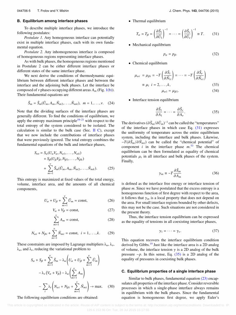
We next derive the conditions of thermodynamic equi-librium between different interface phases and between theinterface and the adjoining bulk phases. Let the interface becomposed of ν phases occupying different areas Am (Fig. 1(b)).Their fundamental equations are

Sm = Sm(Um, Am, Nm2, . . . , Nmk), m = 1, . . . , ν. (24)

Note that the dividing surfaces of the interface phases aregenerally different. To find the conditions of equilibrium, weapply the entropy maximum principle19–21 with respect to thetotal entropy of the system considered to be isolated. Thecalculation is similar to the bulk case (Sec. II C), exceptthat we now include the contributions of interface phasesthat were previously ignored. The total entropy combines thefundamental equations of the bulk and interface phases,

Stot = Sα(UαVα,Nα1, . . . ,Nαk)+ Sβ(UβVβ,Nβ1, . . . ,Nβk)

+

νm=1

Sm(Um, Am, Nm2, . . . , Nmk). (25)

This entropy is maximized at fixed values of the total energy,volume, interface area, and the amounts of all chemicalcomponents,

Uα +Uβ +

νm=1

Um = const, (26)

Vα + Vβ = const, (27)ν

m=1

Am = const, (28)

Nαi + Nβi +

νm=1

Nmi = const, i = 1, . . . , k . (29)

These constraints are imposed by Lagrange multipliers λu, λv,λa, and λi, reducing the variational problem to

Sα + Sβ +

νm=1

Sm − λu *,Uα +Uβ +

νm=1

Um+-

− λv�Vα + Vβ

�− λa *

,

νm=1

Am+-

−i

λi *,

Nαi + Nβi +

νm=1

Nmi+-→ max. (30)

The following equilibrium conditions are obtained:

• Thermal equilibrium

Tα = Tβ =

(∂ S1

∂U1

)−1

= · · · =(∂ Sν∂Uν

)−1

≡ T. (31)

• Mechanical equilibrium

pα = pβ. (32)

• Chemical equilibrium

µαi = µβi = −T(∂ S1

∂ N1i

)= · · · = −T

(∂ Sν∂ Nνi

)≡ µi i = 2, . . . , k, (33)

µα1 = µβ1. (34)

• Interface tension equilibrium

∂ S1

∂A1= · · · = ∂ Sν

∂Aν. (35)

The derivatives (∂ Sm/∂Um)−1 can be called the “temperatures”of the interface phases in which case Eq. (31) expressesthe uniformity of temperature across the entire equilibriumsystem, including the interface and bulk phases. Likewise,−T(∂ Sm/∂ Nmi) can be called the “chemical potential” ofcomponent i in the interface phase m.53 The chemicalequilibrium can be then formulated as equality of chemicalpotentials µi in all interface and bulk phases of the system.Finally,

γm ≡ −T∂ Sm

∂Am(36)

is defined as the interface free energy or interface tension ofphase m. Since we have postulated that the excess entropy is ahomogeneous function of first degree with respect to the area,it follows that γm is a local property that does not depend onthe area. For small interface regions bounded by other defects,this may not be the case. Such situations are not considered inthe present theory.

Thus, the interface tension equilibrium can be expressedas the equality of tensions in all coexisting interface phases,

γ1 = · · · = γν. (37)

This equation recovers the interface equilibrium conditionderived by Gibbs.19 Just like the interface area is a 2D analogof volume, the interface tension γ is a 2D analog of the bulkpressure −p. In this sense, Eq. (35) is a 2D analog of theequality of pressures in coexisting bulk phases.

C. Equilibrium properties of a single interface phase

Similar to bulk phases, fundamental equation (23) encap-sulates all properties of the interface phase. Consider reversibleprocesses in which a single-phase interface always remainsin equilibrium with the bulk phases. Since the fundamentalequation is homogeneous first degree, we apply Euler’s

This article is copyrighted as indicated in the article. Reuse of AIP content is subject to the terms at: http://scitation.aip.org/termsconditions. Downloaded to IP:

129.6.153.96 On: Tue, 28 Jul 2015 15:17:55

044706-6 T. Frolov and Y. Mishin J. Chem. Phys. 143, 044706 (2015)

theorem to obtain

S =∂ S∂U

U +∂ S∂A

A +ki=2

∂ S∂ Ni

Ni

=1T

U − γ

TA − 1

T

ki=2

µi Ni, (38)

which can be rewritten as

γA = U − T S −ki=2

µi Ni. (39)

This equation appears in Gibbs (Ref. 19, Eq. (502)) and ex-presses γ as the excess of the grand potential U − T S − Σiµi Ni

per unit interface area. On the other hand, differentiation offundamental equation (23) gives

dS =1T

dU − γ

TdA − 1

T

ki=2

µidNi (40)

from which

dU = TdS +ki=2

µidNi + γdA. (41)

This well-known equation also appears in Gibbs (Ref. 19, Eq.(501)) and shows that the interface adds an extra work termwhich is a 2D analog of the mechanical work −pdV in bulksystems. In fact, this equation was the starting point of Gibbs’interface thermodynamics from which all other equations werederived. Finally, by adding Eq. (41) to the differential ofEq. (39), we obtain the Gibbs adsorption equation (Ref. 19,Eq. (508))

Adγ = −SdT −ki=2

Nidµi. (42)

Note the ease with which these equations have been derivedstarting from the fundamental equation and using knownproperties of homogeneous functions.

Equation (42) shows that the state of a single-phaseinterface that maintains equilibrium with the bulk phases isdefined by k independent intensive variables. This is consistentwith Gibbs phase rule (21) predicting f = k degrees offreedom for a two-phase (ϕ = 2) system with k chemicalcomponents.

D. Reformulation in generalized interface excesses

Until this point, the interface excess quantities weredefined relative to a certain choice of the dividing surface. Wecan now remove this restriction and reformulate all equationsin terms of generalized excess introduced by Cahn.40 Westart with adsorption equation (42) and replace all excessesappearing in this equation by their definitions according toEq. (22). As a result, the adsorption equation takes the “global”form

Adγ = −SdT + V dp −ki=1

Nidµi, (43)

where S, V , and Ni refer to the entire system containing twobulk phases and the interface. The terms with Xα and Xβ

canceled out due to the Gibbs-Duhem equations for the bulkphases,

0 = −SαdT + Vαdp −ki=1

Nαidµi, (44)

0 = −SβdT + Vβdp −ki=1

Nβidµi. (45)

Since these equations remain valid after re-scaling by anarbitrary factor, they can be thought of as representing arbi-trarily chosen homogeneous regions inside the bulk phases.Note that global adsorption equation (43) does not containexcess quantities, which demonstrates that γ is independentof definitions of excesses.

As a result of this “unwrapping” procedure, adsorptionequation (42) has been recast in global form (43) where it doesnot depend on any definitions of interface excesses. However,this equation must be considered simultaneously with Gibbs-Duhem equations (46) and (45). The advantage of this globalform is that we can now eliminate any two differentials fromEq. (43), not necessarily dp and dµ1 as it was done beforeby choosing the equimolar dividing surface of component 1.The elimination is accomplished most elegantly by using theKramer rule of linear algebra,40 resulting in the generalizedadsorption equation

Adγ = −[S]XYdT + [V ]XYdp −ki=1

[Ni]XYdµi. (46)

Here, X and Y are any two extensive variables from the list(S,V,N1, . . . ,Nk) and the square brackets denote ratios of twodeterminants. Namely, for any extensive property Z ,

[Z]XY ≡

���������

Z X YZα Xα YαZβ Xβ Yβ

���������������

Xα YαXβ Yβ

������

, (47)

where Z , X , and Y are computed for the two-phase systemand the remaining quantities represent arbitrarily chosenhomogeneous regions inside the bulk phases. The generalizedexcess [Z]XY has the meaning of the interface excess of theextensive property Z in a two-phase system that contains thesame amounts of X and Y as the two single-phase regionscombined. By properties of determinants, [X]XY = [Y ]XY = 0.Thus, the excesses of X and Y are zero and two terms inEq. (46) automatically vanish. By choosing the properties Xand Y , we can control which two differentials in Eq. (46)disappear and which k remain as independent variables.

If X is volume, then [Z]XY defines an excess of Zrelative to a geometric dividing surface as in Gibbs’ interfacethermodynamics.19 The position of the dividing surface is thendictated by the choice of the second variable Y . For example,by choosing Y = N1, we return to the previously definedexcesses relative to the equimolar surface of component 1.When neither X nor Y is volume, the generalized interface

This article is copyrighted as indicated in the article. Reuse of AIP content is subject to the terms at: http://scitation.aip.org/termsconditions. Downloaded to IP:

129.6.153.96 On: Tue, 28 Jul 2015 15:17:55

044706-7 T. Frolov and Y. Mishin J. Chem. Phys. 143, 044706 (2015)

excess is defined without using any dividing surface. Thisgeneralization enables us to define interface excess volume[V ]XY . As all other excesses, the excess volume is not unique.For example, if we choose X = S and Y = N1, the excessvolume becomes

[V ]SN1=

���������

V S N1

Vα Sα Nα1

Vβ Sβ Nβ1

���������������

Sα Nα1

Sβ Nβ1

������

. (48)

Other interface properties can also be reformulated interms for generalized excesses. For example, the interfacetension equation (39) can be generalized to41

γA = [U]XY − T[S]XY + p[V ]XY −ki=1

µi[Ni]XY . (49)

This leads to several equivalent excess formulations of γ, suchas

γA =U + pV −

ki=2

Niµi

SN1

=

U − T S + pV −

ki=3

Niµi

N1N2

. (50)

We can also derive an interface analog of the Clapeyron-Clausius equation describing phase coexistence. Indeed, fortwo coexisting interface phase, labeled by a single and doubleprime, Eq. (46) takes the form

dγ′ = − [S′]XY

A′dT +

[V ′]XY

A′dp −

ki=1

�N ′i

�XY

A′dµi, (51)

dγ′′ = − [S′′]XY

A′′dT +

[V ′′]XY

A′′dp −

ki=1

�N ′′i

�XY

A′′dµi. (52)

In reversible processes when the phases remain in equilibriumwith each other, their tensions must remain equal, dγ′ = dγ′′.This immediately gives

−∆( [S]XY

A

)dT + ∆

( [V ]XY

A

)dp

−ki=1

∆

( [Ni]XY

A

)dµi = 0, (53)

where ∆ denotes the difference between the two interfacephases. For example, by choosing X = S and Y = V , we obtainthe Clapeyron-Clausius type equation

−ki=1

∆

( [Ni]XY

A

)dµi = 0, (54)

defining a (k − 1)-dimensional hypersurface of interfacephase coexistence in the k-dimensional space of variables(µ1, . . . , µk). The coefficients in Eq. (54) are the jumps ofinterface segregations (per unit area) across this hypersurface.

E. The interface phase rule

We can now formulate the interface phase rule. Consideran equilibrium heterogeneous system composed of ϕ co-existing bulk phases. We will focus the attention on oneparticular interface separating two phases. Suppose thisinterface contains ν coexisting interface phases. We wish tofind the number of independent variables that can be variedwhile keeping the same number of bulk and interface phases.Let us call this number f i degrees of freedom.

The system is described by (k + 2) intensive parameters:T , p, and k chemical potentials µi. But they are notindependent. First, we have ϕ Gibbs-Duhem equations (20)for the bulk phases that impose ϕ constraints on variationsof intensities. Second, we have ν adsorption equations forthe coexisting interface phases. They contain an additionalvariable γ, which we can eliminate and obtain (ν − 1)equations of constraint. As a result, the number of degreesof freedom is (k + 2) − ϕ − (ν − 1). The interface phase rulebecomes

f i = k + 3 − ϕ − ν. (55)

From this rule, we can find the maximum possible numberof coexisting interface phases (when f i = 0),

νmax = k + 3 − ϕ. (56)

For example, in a single-component two-phase system, onlytwo interface phases can co-exist at the interface. At a triplepoint (ϕ = 3), only one phase can exist at each interface. Onthe other hand, if we have a binary single-phase system, aninterface such as a surface can support up to four coexistinginterface phases.

IV. LINE PHASES

A. Definition of a line phase

In the analysis of coexisting interface phases, we haveso far neglected the contributions of the line defects lying inthe interface plane and separating interface phases. Such linedefects, or simply lines, are 1D analogs of phase boundariesin bulk thermodynamics. We are not aware of experimentalstudies of lines, but they have recently been observed inatomistic computer simulations of metallic grain boundaries.10

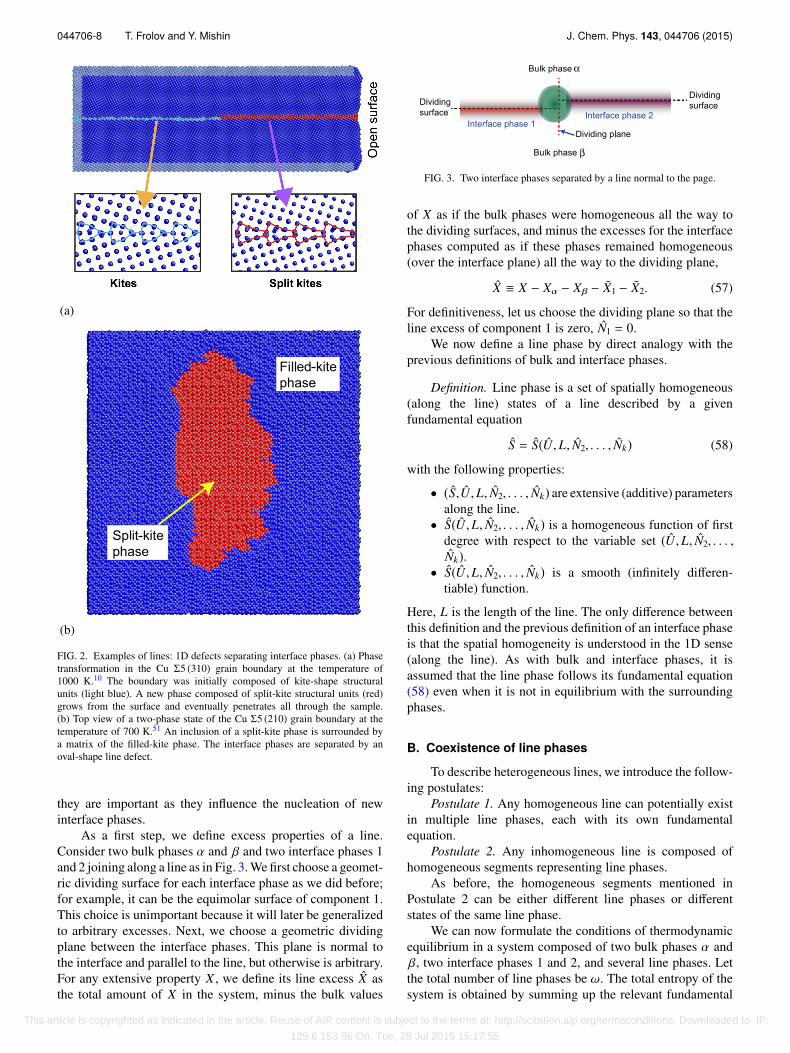
Fig. 2(a) shows an example of a straight line separating twograin boundary phases, called filled kites and split kites, in asymmetrical tilt boundary in Cu. The structure of this grainboundary undergoes a reversible transformation from onephase to another with temperature. At some temperature, thetwo phases coexist in equilibrium and are separated by a line. Itis also possible to equilibrate and isolated inclusion of the split-kite phase bounded by a curved line (Fig. 2(b)). The oval shapeof the line indicates that its properties are anisotropic. Theseobservations motivate the development of a thermodynamictheory of lines. Similar to bulk and interface phases, one canexpect that lines may exist in multiple phases. The goal of thissection is to examine thermodynamic properties of line phases.It should be noted that line phases were not discussed byGibbs19 or analyzed by other researchers after Gibbs. However,

This article is copyrighted as indicated in the article. Reuse of AIP content is subject to the terms at: http://scitation.aip.org/termsconditions. Downloaded to IP:

129.6.153.96 On: Tue, 28 Jul 2015 15:17:55

044706-8 T. Frolov and Y. Mishin J. Chem. Phys. 143, 044706 (2015)

FIG. 2. Examples of lines: 1D defects separating interface phases. (a) Phasetransformation in the Cu Σ5 (310) grain boundary at the temperature of1000 K.10 The boundary was initially composed of kite-shape structuralunits (light blue). A new phase composed of split-kite structural units (red)grows from the surface and eventually penetrates all through the sample.(b) Top view of a two-phase state of the Cu Σ5 (210) grain boundary at thetemperature of 700 K.51 An inclusion of a split-kite phase is surrounded bya matrix of the filled-kite phase. The interface phases are separated by anoval-shape line defect.

they are important as they influence the nucleation of newinterface phases.

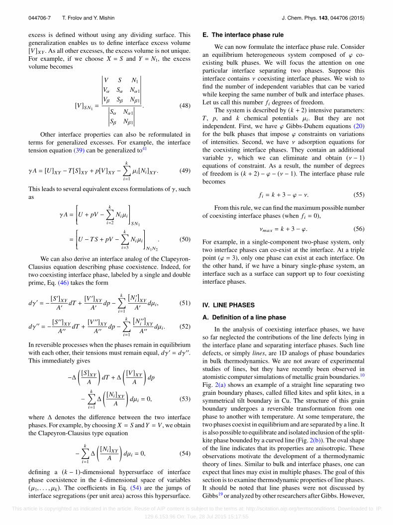
As a first step, we define excess properties of a line.Consider two bulk phases α and β and two interface phases 1and 2 joining along a line as in Fig. 3. We first choose a geomet-ric dividing surface for each interface phase as we did before;for example, it can be the equimolar surface of component 1.This choice is unimportant because it will later be generalizedto arbitrary excesses. Next, we choose a geometric dividingplane between the interface phases. This plane is normal tothe interface and parallel to the line, but otherwise is arbitrary.For any extensive property X , we define its line excess X asthe total amount of X in the system, minus the bulk values

FIG. 3. Two interface phases separated by a line normal to the page.

of X as if the bulk phases were homogeneous all the way tothe dividing surfaces, and minus the excesses for the interfacephases computed as if these phases remained homogeneous(over the interface plane) all the way to the dividing plane,

X ≡ X − Xα − Xβ − X1 − X2. (57)

For definitiveness, let us choose the dividing plane so that theline excess of component 1 is zero, N1 = 0.

We now define a line phase by direct analogy with theprevious definitions of bulk and interface phases.

Definition. Line phase is a set of spatially homogeneous(along the line) states of a line described by a givenfundamental equation

S = S(U,L, N2, . . . , Nk) (58)

with the following properties:

• (S,U,L, N2, . . . , Nk) are extensive (additive) parametersalong the line.

• S(U ,L, N2, . . . , Nk) is a homogeneous function of firstdegree with respect to the variable set (U,L, N2, . . . ,Nk).

• S(U ,L, N2, . . . , Nk) is a smooth (infinitely differen-tiable) function.

Here, L is the length of the line. The only difference betweenthis definition and the previous definition of an interface phaseis that the spatial homogeneity is understood in the 1D sense(along the line). As with bulk and interface phases, it isassumed that the line phase follows its fundamental equation(58) even when it is not in equilibrium with the surroundingphases.

B. Coexistence of line phases

To describe heterogeneous lines, we introduce the follow-ing postulates:

Postulate 1. Any homogeneous line can potentially existin multiple line phases, each with its own fundamentalequation.

Postulate 2. Any inhomogeneous line is composed ofhomogeneous segments representing line phases.

As before, the homogeneous segments mentioned inPostulate 2 can be either different line phases or differentstates of the same line phase.

We can now formulate the conditions of thermodynamicequilibrium in a system composed of two bulk phases α andβ, two interface phases 1 and 2, and several line phases. Letthe total number of line phases be ω. The total entropy of thesystem is obtained by summing up the relevant fundamental

This article is copyrighted as indicated in the article. Reuse of AIP content is subject to the terms at: http://scitation.aip.org/termsconditions. Downloaded to IP:

129.6.153.96 On: Tue, 28 Jul 2015 15:17:55

044706-9 T. Frolov and Y. Mishin J. Chem. Phys. 143, 044706 (2015)

equations

Stot = Sα(Uα,Vα,Nα1, . . . ,Nαk)+ Sβ(Uβ,Vβ,Nβ1, . . . ,Nβk)+ S1(U1, A1, N12, . . . , N1k)+ S2(U2, A2, N22, . . . , N2k)+

ωn=1

Sn(Un,Ln, Nn2, . . . , Nnk). (59)

In an isolated system, variations of Stot are subject to theconstraints of fixed total energy, total volume, total area ofthe interface phases, total length of the line phases, and thetotal amount of each chemical component,

Uα +Uβ + U1 + U2 +

ωn=1

Un = const, (60)

Vα + Vβ = const, (61)A1 + A2 = const, (62)ωn=1

Ln = const, (63)

Nαi + Nβi + N1i + N2i +

ωn=1

Nni = const, i = 1, . . . , k . (64)

Imposing these constraints by appropriate Lagrange multi-pliers, the necessary conditions of Stot → max are summarizedas follows:

• Thermal equilibrium

Tα = Tβ =

(∂ S1

∂U1

)−1

=

(∂ S2

∂U2

)−1

=

(∂ S1

∂U1

)−1

= · · · =(∂ Sω∂Uω

)−1

≡ T. (65)

• Mechanical equilibrium

pα = pβ. (66)

• Chemical equilibrium

µαi = µβi = −T(∂ S1

∂ N1i

)= −T

(∂ S2

∂ N2i

)= −T

(∂ S1

∂ N1i

)= · · · = −T

(∂ Sω∂ Nωi

)≡ µi i = 2, . . . , k, (67)

µα1 = µβ1. (68)

• Interface tension equilibrium

∂ S1

∂A1=

∂ S2

∂A2. (69)

• Line tension equilibrium

∂ S1

∂L1= · · · = ∂ Sω

∂Lω. (70)

Equation (65) expresses the uniformity of temperature acrossthe equilibrium system, including the bulk, interface, and linephases. It is convenient to call the derivative −T(∂ Sn/∂ Nni)the “chemical potential” of component i in the line phase n.

Then the chemical equilibrium condition can be formulatedas equality of chemical potentials µi in the bulk, interfaceand line phases. Interface tension equilibrium condition (69)reduces to γ1 = γ2. Finally, we define the line tension of a linephase n by

τn = −T∂ Sn∂Ln

. (71)

Eq. (70) states that the line tensions of coexisting line phasesmust be equal,

τ1 = · · · = τω. (72)

The line tension is obviously a 1D analog of the bulk pressure(up to the sign) and the interface tension γ.

C. The line adsorption equation

Returning to a single line phase, consider reversible ther-modynamic processes in which the line remains in equilibriumwith the interface and bulk phases. Applying, as usual, theEuler theorem to fundamental equation (58), we have

S =∂ S

∂UU +

∂ S∂L

L +ki=2

∂ S

∂ Ni

Ni

=1T

U − τ

TL − 1

T

ki=2

µi Ni (73)

from which

τL = U − T S −ki=1

µi Ni. (74)

On the other hand, differentiation of fundamental equation(58) gives

dS =1T

dU − τ

TdL − 1

T

ki=2

µidNi, (75)

and thus

dU = TdS +ki=2

µidNi + τdL. (76)

Finally, adding Eq. (76) to the differential of Eq. (74), weobtain the Gibbs adsorption equation for a line phase,

Ldτ = −SdT −ki=2

Nidµi. (77)

Equations (73)–(77) bear a close similarity with respectiveequations (38)–(42) of interface thermodynamics. This isnot surprising given the similar structures of fundamentalequations (23) and (58) defining the interface and line phases,respectively.

D. Reformulation in generalized line excesses

The k differentials appearing in line adsorption equation(77) are not all independent because we have not yet imposedthe condition of equality of the surface tensions of the interfacephases separated by the line. The latter condition reduces the

This article is copyrighted as indicated in the article. Reuse of AIP content is subject to the terms at: http://scitation.aip.org/termsconditions. Downloaded to IP:

129.6.153.96 On: Tue, 28 Jul 2015 15:17:55

044706-10 T. Frolov and Y. Mishin J. Chem. Phys. 143, 044706 (2015)

number of independent differentials to (k − 1). To express theadsorption equation in terms of independent differentials, wewill reformulate it in terms of generalized excesses.

The first step is to “unwrap” Eq. (77) by replacing allexcess quantities by their definitions (57). After rearrange-ments with the aid of Eqs. (9) and (42), we obtain the globalform of the line adsorption equation

Ldτ = −SdT + V dp −ki=1

Nidµi − Adγ. (78)

Here, the quantities S, V , Ni, and A refer to an arbitrarilychosen rectangular box containing the two interface phasesand the line (Fig. 4(a)). The dimensions of the box must bemuch larger than the characteristic thickness of the interfaceand the cross-section of the line. Equation (78) shows thatτ is independent of definitions of excesses. It must besupplemented by four other equations containing the samedifferentials, namely, the global forms of the adsorptionequations for the interface phases,

0 = −S′dT + V ′dp −ki=1

N ′idµi − A′dγ, (79)

0 = −S′′dT + V ′′dp −ki=1

N ′′i dµi − A′′dγ, (80)

and the Gibbs-Duhem equations for the bulk phases,

0 = −SαdT + Vαdp −ki=1

Nαidµi, (81)

0 = −SβdT + Vβdp −ki=1

Nβidµi. (82)

Equations (79) and (80) are written for imaginary boxescontaining a single interface phase, either 1 or 2, anduninfluenced by the line (Figs. 4(b) and 4(c)). The cross-sectional areas and the total amounts of extensive propertiesin these boxes are distinguished by the prime and doubleprime, respectively. Likewise, Eqs. (81) and (82) representhomogeneous bulk regions of phases α and β, respectively(Fig. 4(d)). Because the differential coefficients in each ofthe Eqs. (78)–(82) can be scaled by an arbitrary commonmultiplier, the choice of dimensions of all boxes is arbitraryas long as the conditions stated above (e.g., the homogeneityof the bulk regions) are satisfied.

The right-hand side of Eq. (78) contains (k + 3) terms.Equations (79)–(82) impose four constraints, leaving (k − 1)independent differentials as the variables of τ. Which variablesto eliminate is a matter choice and can be convenientlycontrolled by re-writing Eq. (78) in terms of generalized excessas it was done for interfaces (Sec. III D). Applying the Kramerrule of linear algebra,40 we obtain

Ldτ = −[S]WXYZdT + [V ]WXYZdp

−ki=1

[Ni]WXYZdµi − [A]WXYZdγ, (83)

where W , X , Y , and Z are any four of the extensive variables(S,V,N1, . . . ,Nk, A). The square brackets are generalized

FIG. 4. Reference boxes used for the calculation of line excess properties.(a) Two interface phases separated by a line. (b) Interface phase 1. (c)Interface phase 2. (d) Bulk phases α and β. The values of an extensiveproperty X are indicated next to the boxes.

excesses defined by ratios of two determinants of ranks 5and 4. Namely, for any extensive property R,

[R]WXYZ ≡

��������������

R W X Y ZR′′ W ′′ X ′′ Y ′′ Z ′′

R′ W ′ X ′ Y ′ Z ′

Rα Wα Xα Yα Zα

Rβ Wβ Xβ Yβ Zβ

�������������������������

W ′′ X ′′ Y ′′ Z ′′

W ′ X ′ Y ′ Z ′

Wα Xα Yα Zα

Wβ Xβ Yβ Zβ

�����������

. (84)

The meaning of [R]WXYZ is the line excess of property Rcomputed with a set of reference boxes such that the excessesof W , X , Y , and Z are zero. Equation (83) reveals two newexcess quantities that did not appear in Eq. (77): the line excessvolume [V ]WXYZ characterizing the contribution of the lineto the total interface excess volume, and the line excess area[A]WXYZ characterizing the interface area attributed to theline. Equation (83) shows that a line tension depends on both

This article is copyrighted as indicated in the article. Reuse of AIP content is subject to the terms at: http://scitation.aip.org/termsconditions. Downloaded to IP:

129.6.153.96 On: Tue, 28 Jul 2015 15:17:55

044706-11 T. Frolov and Y. Mishin J. Chem. Phys. 143, 044706 (2015)

the 3D pressure p and the 2D “pressure” γ. The line excessvolume and area, as well as the line excess entropy [S]WXYZ

and the line segregations [Ni]WXYZ, are not unique. Theirvalues depend on the choice of the properties W , X , Y , and Z .Whatever their choice is, the terms with the excesses of W , X ,Y , and Z disappear and we are left with (k − 1) independentdifferentials. For example, by choosing W XY Z = ASV N1, theline adsorption equation reduces to

Ldτ = −ki=2

[Ni]ASVN1dµi, (85)

involving only line segregations.The excess form of the line tension, which was previously

given by Eq. (74), can also be generalized to

τL = [U]WXYZ − T[S]WXYZ + p[V ]WXYZ

−ki=1

µi[Ni]WXYZ − [A]WXYZγ. (86)

For example, the choice of W XY Z = ASV N1 reduces thisequation to

τL =U −

ki=2

µiNi

ASVN1

. (87)

As an application of Eq. (83), consider two coexistingline phases that remain in equilibrium with each other during areversible process. Writing Eq. (83) for each phase, subtractingthese equations, and taking into account that the differentialsdτ remain equal for both phases, we obtain

− ∆( [S]WXYZ

L

)dT + ∆

( [V ]WXYZ

L

)dp

−ki=1

∆

( [Ni]WXYZ

L

)dµi − ∆

( [A]WXYZ

L

)dγ = 0. (88)

Here, the symbol ∆ designates the difference between theexcess properties (per unit length) of the two line phase. Thisequation describes a (k − 2)-dimensional phase coexistencehypersurface in the (k − 1)-dimensional space of variablesand is analogous to the Clapeyron-Clausius equation forcoexisting bulk systems. For example, for W XY Z = ASV N1,the coexistence hypersurface exists is the space of chemicalpotentials (µ2, . . . , µk) and is described by the equation

ki=2

∆

( [Ni]WXYZ

L

)dµi = 0, (89)

where the differential coefficients are the jumps in linesegregations (per unit length) across the hypersurface.

E. The line phase rule

Consider an equilibrium system containing ϕ bulk phasesthat we want to keep during all reversible variations ofparameters. We single out one particular interface containingν interface phases and consider a particular line between twointerface phases 1 and 2. Suppose this line contains ω linephases. How many variables can we vary while keeping allthese phases in coexistence?

Out of the (k + 2) intensities of our system, ϕ can beeliminated by the Gibbs-Duhem equations for the bulk phases.The adsorption equations for the interface phases impose νmore constraints. The adsorption equations for the line phasesadd another ω constraints. However, the interface and lineadsorption equations contain the additional differentials dγand dτ. Eliminating them, the total number of constraintsbecomes (ϕ + ν + ω − 2). Thus, the number of remainingdegrees of freedom is

fL = k + 4 − ϕ − ν − ω. (90)

This equation is the phase rule for line phases. The maximumpossible number of coexisting line phases (when fL = 0) is

ωmax = k + 4 − ϕ − ν. (91)

If we are only concerned with two bulk phases separatedby an interface containing one line, then ϕ = 2, ν = 2, and thephase rule reduces to fL = k − ω. Accordingly, the maximumnumber of coexisting line phases is ωmax = k.

V. DISCUSSION

Table I summarizes the phase rules derived here for thebulk, interface, and line phases. The last column contains themaximum number of phases that can coexist in equilibrium.All these phase rules can be summarized in the equations

f = k + 5 − d − θ, (92)θmax = k + 5 − d, (93)

where d is the smallest dimensionality of phases included intoconsideration and θ = ϕ + ν + ω is the number of coexistingphases in the system. For a given d, the number of phases of alower dimensionality must be excluded from θ. For example,ω = 0 for interface phases (Table I).

These equations can be used to predict the number ofindependent variables and the maximum possible number ofcoexisting phases, depending on the dimensionality of thephases. For example, in a binary system, a phase boundary cansupport a maximum of νmax = 3 coexisting interface phases(d = 2, k = 2, ϕ = 2, andω = 0). If pressure is fixed, then onlytwo. In a single-component system, an interface can supportonly two interface phases and the line separating them canhave only one line phase (d = 1, k = 1, ϕ = 2, and ν = 2).

In the foregoing discussion, we assumed that interfacesand lines separated distinct phases. This analysis is readilyextended to single-phase interfaces such as grain boundariesand lines separating regions of the same interface phasewith different crystallographic orientations. In such cases,the choice of the dividing surface is arbitrary and allexcesses N1, . . . , Nk (accordingly, N1, . . . , Nk) must appearas arguments in the fundamental equations. All calculationsremain similar and lead to the same phase rules with anappropriate count of phases (e.g., ϕ = 1 for a grain boundary).

Using the same thermodynamic approach, it is straightfor-ward to derive a phase rule for 0-dimensional defects formedbetween neighboring line phases (Fig. 1(b)), which could becalled “points.”

This article is copyrighted as indicated in the article. Reuse of AIP content is subject to the terms at: http://scitation.aip.org/termsconditions. Downloaded to IP:

129.6.153.96 On: Tue, 28 Jul 2015 15:17:55

044706-12 T. Frolov and Y. Mishin J. Chem. Phys. 143, 044706 (2015)

TABLE I. Summary of phase rules for bulk, interface, and line phases. k is the number of chemical components,ϕ is the number of bulk phases, ν is the number of interface phases, ω is the number of line phases, and f is thenumber of degrees of freedom.

Bulk phases Interface phases Line phases f Maximum No. of phases

Bulk ϕ 0 0 k +2−ϕ k +2Interface ϕ ν 0 k +3−ϕ−ν k +3−ϕLine ϕ ν ω k +4−ϕ−ν−ω k +4−ϕ−ν

The analysis presented here was based on a simplifiedtreatment and its immediate applications are restricted tomulticomponent fluids. This treatment is not applicable tosolid phases without appropriate modifications.33–35,42–45 Inter-faces in solid systems are often anisotropic and their propertiesmay depend on the crystallographic orientation of the interfaceplane. In terms of Cahn’s classification,3 all interface phasetransformations considered here are congruent. Furthermore,we identified the interface free energy with the interface stressand referred to this common property as “tension.” Whilethis is correct for fluid systems, for solid-solid interfaces,the interface free energy and interface stress are differentquantities both conceptually and numerically.19,40,42–47 A linephase can also be characterized by a line free energy and a linestress, which are different properties. We neglected chemicalreactions in the bulk or at interfaces and lines. Finally, for thesake of simplicity, we neglected the curvature effects on theinterface and line properties. The goal of the present work wasto demonstrate the general approach and outline the directionof future work. Extensions of the present analysis to includethe effects mentioned above are possible and would result inthermodynamic theories and phase rules for low-dimensionalphases in a wider range of real materials. The nucleation ofnew interface phases is not well understood or theoreticallydescribed. Developing a more detailed thermodynamic theoryof lines is the first necessary step in this direction. Much canbe done in this field.

It should be clarified that the proposed approach doesnot ignore the fundamental differences in physical propertiesof low-dimensional versus bulk phases. In fact, phase rules(92) and (93) derived here contain the dimensionality of thesystem as a parameter. Bulk phases, interfaces, and linesbelong to different universality classes and exhibit differentcritical behaviors (e.g., critical exponents), as well as manyother physical properties.6 However, the basic thermodynamicformalism and the rules for the identification of independentthermodynamic variables and description of phase equilibriaremain exactly the same for any dimensionality of space.In its postulational basis, thermodynamics is blind to thedimensionality of space. The postulates of thermodynamicsare formulated in abstract concepts such as a system, astate, a variable, extensive and intensive parameters, andconservation21 that do not involve the real space or itsdimensionality. As a consequence, the fundamental equationof any phase has the same mathematical structure regardlessof whether the phase exists in 3D space, at an interface or ina line defect. This explains the remarkable similarity, in factidentity, in the phase equilibrium descriptions for the bulk andlow-dimensional systems.

While the concepts of 2D phases and 2D phase diagramshave long been accepted and successfully used in thesurface/interface physics and chemistry communities andwere later adopted in materials science,2,3,5 a recent trendin the materials community is to reject the terms “interfacephase” and “2D phase” on the ground that such phases“do not satisfy the Gibbs definition of a phase.”13–17 It ispointed out that they do not meet Gibbs’ requirement ofhomogeneity and in addition cannot exist without being incontact with bulk phases. Gibbs’ definition of a phase19 wasdiscussed in Sec. II A. Mathematically, his requirement ofhomogeneity is expressed by the homogeneity of first degreeof the fundamental equation of the phase. For interfaces, thefundamental equation is homogeneous with respect to the area,and for lines with respect to the length. In other words, thehomogeneity of a phase is embedded in its definition (4)for any dimensionality. The requirement that we should beable to physically extract any given phase from the rest ofthe system is not part of Gibbs’ thermodynamics.19 Is it notpart of the modern logical structure of thermodynamics either,nor is it needed for any thermodynamic derivations involvingphases. As long as a particular part of a system follows its ownfundamental equation satisfying the mathematical propertiesstated above and can exchange extensive properties with therest of the system, it satisfies the thermodynamic definition ofa phase.

VI. CONCLUSIONS

To summarize, we have presented a unified thermody-namic description of phases and phase equilibria in 3D, 2D,and 1D systems. In all cases, the phase is identified with afundamental equation of state, see Eq. (4). The fundamentalequation defines a phase and encapsulates all of its properties.In all dimensions, the phases are treated the same way andare described by similar thermodynamic equations. The samethermodynamic formalism can be applied for the descriptionof phase equilibria and phase transformations in bulk systems,interfaces, and line defects separating 2D interface phases.For both lines and interfaces, we have rigorously derivedadsorption equations in terms of generalized excess quantities.We have also derived phase coexistence equations that canbe utilized for the construction of phase diagrams for low-dimensional systems. The Gibbs phase rule describing thecoexistence of bulk phases has been generalized to phaserules for interfaces and lines. Such rules predict the number ofthermodynamic degrees of freedom and the maximum numberof phases that can coexist in the systems of the respectivedimensionality.

This article is copyrighted as indicated in the article. Reuse of AIP content is subject to the terms at: http://scitation.aip.org/termsconditions. Downloaded to IP:

129.6.153.96 On: Tue, 28 Jul 2015 15:17:55

044706-13 T. Frolov and Y. Mishin J. Chem. Phys. 143, 044706 (2015)

Recent years have seen a significant increase in theresearch activity dedicated to interface phase transformations.Experiments have uncovered a number grain boundary phaseswith discrete thicknesses and various segregation patterns inbinary and multi-component metallic alloys17,48,49 and ceramicmaterials.15–17 It has been demonstrated that transformationsamong such phases can strongly impact many engineeringproperties of materials such as grain growth, mechanical be-havior, and interface transport.50 On the modeling side,atomistic simulations have revealed reversible temperature-induced transformations between different structural phasesin metallic systems10 and their effect on grain boundarydiffusion,11 response to applied mechanical stresses,12 andother properties. Phases inside line defects have never beenreported by either experimentalists or modelers. However, weenvision that such phases may be discovered in the future. Thepresent work predicts their possible existence and describesthe conditions of their thermodynamic coexistence. It shouldbe emphasized that lines play a critical role in 2D phasetransitions. For example, their excess free energy and otherproperties determine the nucleation barriers of 2D phases asillustrated by Fig. 2.

At this juncture, it is important to develop theories capableof explaining the experimental observations and simulationresults and guiding new research in this field. It is hoped thatthe present work contributes to this course by providing arigorous thermodynamic framework for the description andprediction of phase equilibria in interfaces and lines. Asone example, the phase rules derived in this work providea guidance for phase diagram construction and design ofnew experiments and simulations, as usually does the existingphase rule for bulk systems.

ACKNOWLEDGMENTS

T.F. was supported by a post-doctoral fellowship fromthe Miller Institute for Basic Research in Science at theUniversity of California, Berkeley. Y.M. was supported by theNational Science Foundation, Division of Materials Research,the Metals and Metallic Nanostructures Program.

1A. P. Sutton and R. W. Balluffi, Interfaces in Crystalline Materials (Claren-don Press, Oxford, 1995).

2E. W. Hart, “Grain boundary phase transformations,” in Nature andBehavior of Grain Boundaries, edited by H. Hu (Plenum, New York, 1972),pp. 155–170.

3J. W. Cahn, “Transitions and phase equilibria among grain boundary struc-tures,” J. Phys. Colloq. 43, 199–213 (1982).

4R. Pandit, M. Schick, and M. Wortis, “Systematics of multilayer adsorptionphenomena on attractive substrates,” Phys. Rev. B 26, 5112–5140 (1982).

5C. Rottman, “Theory of phase transitions at internal interfaces,” J. Phys.Colloq. 49, 313–322 (1988).

6G. Forgacs, R. Lipowsky, and T. M. Nieuwenhuizen, “The behavior ofinterfaces in ordered and disordered systems,” in Phase Transitions andCritical Phenomena, edited by C. Domb and J. Lebowitz (Academic Press,San Diego, 1991), Vol. 14, pp. 135–364.

7B. B. Straumal and B. Baretzky, “Grain boundary phase transitions and theirinfluence on properties of polycrystals,” Interface Sci. 12, 147–155 (2004).

8Y. Mishin, W. J. Boettinger, J. A. Warren, and G. B. McFadden, “Thermo-dynamics of grain boundary premelting in alloys. I. Phase field modeling,”Acta Mater. 57, 3771–3785 (2009).

9Y. Mishin, M. Asta, and J. Li, “Atomistic modeling of interfaces andtheir impact on microstructure and properties,” Acta Mater. 58, 1117–1151(2010).

10T. Frolov, D. L. Olmsted, M. Asta, and Y. Mishin, “Structural phase trans-formations in metallic grain boundaries,” Nat. Commun. 4, 1899 (2013).

11T. Frolov, S. V. Divinski, M. Asta, and Y. Mishin, “Effect of interface phasetransformations on diffusion and segregation in high-angle grain bound-aries,” Phys. Rev. Lett. 110, 255502 (2013).

12T. Frolov, “Effect of interfacial structural phase transformations on thecoupled motion of grain boundaries: A molecular dynamics study,” Appl.Phys. Lett. 104, 211905 (2014).

13M. Tang, W. C. Carter, and R. M. Cannon, “Diffuse interface model forstructural transitions of grain boundaries,” Phys. Rev. B 73, 024102 (2006).

14M. Tang, W. C. Carter, and R. M. Cannon, “Grain boundary transitions inbinary alloys,” Phys. Rev. Lett. 97, 075502 (2006).

15S. J. Dillon, M. Tang, W. C. Carter, and M. P. Harmer, “Complexion: Anew concept for kinetic engineering in materials science,” Acta Mater. 55,6208–6218 (2007).

16W. D. Kaplan, D. Chatain, P. Wynblatt, and W. C. Carter, “A review ofwetting versus adsorption, complexions, and related phenomena: The rosettastone of wetting,” J. Mater. Sci. 48, 5681–5717 (2013).

17P. R. Cantwell, M. Tang, S. J. Dillon, J. Luo, G. S. Rohrer, and M. P. Harmer,“Grain boundary complexions,” Acta Mater. 62, 1–48 (2013).

18N. Zhou and J. Luo, “Developing grain boundary diagrams for multicompo-nent alloys,” Acta Mater. 91, 202–216 (2015).

19J. W. Gibbs, “On the equilibrium of heterogeneous substances,” in TheCollected Works of J. W. Gibbs (Yale University Press, New Haven, 1948),Vol. 1, pp. 55–349.

20H. B. Callen, Thermodynamics and an Introduction to Thermostatistics, 2nded. (Wiley, New York, 1985).

21L. Tisza, “The thermodynamics of phase equilibrium,” Ann. Phys. 13, 1–92(1961).

22C. Carathéodory, “Untersuchungen über die Grundlagen der Thermody-namik,” Math. Ann. 67, 355–386 (1909).

23P. Ehrenfest and T. Ehrenfest, The Conceptual Foundations of the StatisticalApproach in Mechanics, Dover Books on Physics (Dover, Ithaca, New York,1959).

24P. T. Landsberg, “Main ideas in the axiomatics of thermodynamics,” PureAppl. Chem. 22, 215–227 (1970).

25J. Kestin, “A simple, unified approach to the first and second laws of ther-modynamics,” Pure Appl. Chem. 22, 511–518 (1970).

26C. Gurney, “Principles of classical thermodynamics,” Pure Appl. Chem. 22,519–526 (1970).

27K. A. Masavetas, “The problem of alternative formalisms for the mathemat-ical foundations of chemical thermodynamics,” Math. Comput. Modell. 10,629–635 (1988).

28R. J. J. Jongschaap and H. C. Ottinger, “Equilibrium thermodynamics—Callen’s postulational approach,” J. Non-Newtonian Fluid Mech. 96, 5–17(2001).

29F. Weinhold, Classical and Geometrical Theory of Chemical and PhaseThermodynamics (Wiley, Hoboken, New Jersey, 2009).

30J. S. Rawlinson and B. Widom, Molecular Theory of Capillarity (ClarendonPress, Oxford, 1984).

31J. D. van der Waals, On the Continuity of the Gaseous and Liquid States,Dover Phoenix Editions (Elsevier Science, Mineola, NY, 1988).

32J. W. Cahn and J. E. Hilliard, “Free energy of a nonuniform system. I.Interfacial free energy,” J. Chem. Phys. 28, 258–267 (1958).

33F. Larché and J. W. Cahn, “A linear theory of thermochemical equilibriumof solids under stress,” Acta Metall. 21, 1051–1063 (1973).

34F. C. Larché and J. W. Cahn, “Thermodynamic equilibrium of multiphasesolids under stress,” Acta Metall. 26, 1579–1589 (1978).

35F. C. Larché and J. W. Cahn, “The interactions of composition and stress incrystalline solids,” Acta Metall. 33, 331–367 (1985).

36R. Courant and F. John, Introduction to Calculus and Analysis (SpringerVerlag, New York, 1989), Vol. II.

37R. B. Griffiths and J. C. Wheeler, “Critical points in multicomponent sys-tems,” Phys. Rev. A 2, 1047–1064 (1970).

38D. A. King and D. P. Woodruff, Phase Transitions and Adsorbate Restruc-turing at Metal Surfaces, The Chemical Physics of Solid Surfaces Vol. 7(Elsevier, Amsterdam, Netherlands, 1994).

39D. L. Olmsted, D. Buta, A. Adland, S. M. Foiles, M. Asta, and A. Karma,“Dislocation-pairing transitions in hot grain boundaries,” Phys. Rev. Lett.106, 046101 (2011).

40J. W. Cahn, “Thermodynamics of solid and fluid surfaces,” in InterfaceSegregation, edited by W. C. Johnson and J. M. Blackely (American Societyof Metals, Metals Park, OH, 1979), pp. 3–23.

This article is copyrighted as indicated in the article. Reuse of AIP content is subject to the terms at: http://scitation.aip.org/termsconditions. Downloaded to IP:

129.6.153.96 On: Tue, 28 Jul 2015 15:17:55

044706-14 T. Frolov and Y. Mishin J. Chem. Phys. 143, 044706 (2015)

41T. Frolov and Y. Mishin, “Solid-liquid interface free energy in binary sys-tems: Theory and atomistic calculations for the (110) Cu-Ag interface,” J.Chem. Phys. 131, 054702 (2009).

42T. Frolov and Y. Mishin, “Effect of nonhydrostatic stresses on solid-fluidequilibrium. I. Bulk thermodynamics,” Phys. Rev. B 82, 174113 (2010).

43T. Frolov and Y. Mishin, “Effect of nonhydrostatic stresses on solid-fluid equilibrium. II. Interface thermodynamics,” Phys. Rev. B 82, 174114(2010).

44T. Frolov and Y. Mishin, “Thermodynamics of coherent interfaces undermechanical stresses. I. Theory,” Phys. Rev. B 85, 224106 (2012).

45T. Frolov and Y. Mishin, “Thermodynamics of coherent interfaces undermechanical stresses. II. Application to atomistic simulation of grain bound-aries,” Phys. Rev. B 85, 224107 (2012).

46R. Shuttleworth, “Surface tension of solids,” Proc. Phys. Soc. A 63, 444–457(1950).

47D. Kramer and J. Weissmuller, “A note on surface stress and surface ten-sion and their interrelation via Shuttleworth’s equation and the Lippmannequation,” Surf. Sci. 601, 3042–3051 (2007).

48S. Ma, K. M. Asl, C. Tansarawiput, P. R. Cantwell, M. Qi, M. P. Harmer,and J. Luo, “A grain boundary phase transition in Si–Au,” Scr. Mater. 66,203–206 (2012).

49J. Luo, H. Cheng, K. M. Asl, C. J. Kiely, and M. P. Harmer, “The roleof a bilayer interfacial phase on liquid metal embrittlement,” Science 333,1730–1733 (2011).

50S. V. Divinski, H. Edelhoff, and S. Prokofjev, “Diffusion and segregation ofsilver in copper Σ5 (310) grain boundary,” Phys. Rev. B 85, 144104 (2012).

51T. Frolov, “Grain boundary phase transitions and equilibrium controlled bypoint defects” (to be published).

52A homogeneous state is defined by a set of variables (U, V , N1, . . . , Nk).Two homogeneous states represent the same phase if both satisfy the samefundamental equation.

53The interface chemical potential of component 1 is not defined by Eqs. (33)and (34) since its interface excess is zero. However, we can repeat thecalculation by choosing the dividing surface as equimolar with respect toanother component. This will lead to the expected result that the interfacechemical potential is µ1 = µαi = µβi.

This article is copyrighted as indicated in the article. Reuse of AIP content is subject to the terms at: http://scitation.aip.org/termsconditions. Downloaded to IP:

129.6.153.96 On: Tue, 28 Jul 2015 15:17:55