Ph.D. THESIS Multipolar ordering in f -electron systems Annam´ aria Kiss Supervisor: Prof. Patrik Fazekas Research Institute for Solid State Physics and Optics Department of Theoretical Solid State Physics 2004
Transcript
Ph.D. THESIS
Multipolar ordering in
f-electron systems
Annamaria Kiss
Supervisor: Prof. Patrik Fazekas
Research Institute for Solid StatePhysics and Optics
Orbital ordering phenomena in f -electron systems have been extensivelystudied in the past two decades. The highly degenerate f -shells of rareearth and actinide ions support a great variety of local degrees of freedom:magnetic, quadrupolar and octupolar at least. This leads to variegated andcomplex phase diagrams and magnetic properties. Quadrupolar ordering wasfound to explain the properties of many Ce, Tm and Pr-based rare earth com-pounds like CeB6, TmTe, and PrPb3. The detailed theory of CeB6 containsthe first full symmetry classification of multipoles, including the effect of anexternal magnetic field [5].
In earlier studies, orbital ordering was usually understood to mean justquadrupolar ordering, but it has become clear that orderings of higher mul-tipoles are also realized in some f -electron compounds. Recent experimentalobservations on NpO2 indicate that the primary order parameter of the 25Kphase transition is purely octupole. Multipoles of still higher order, namelyhexadecapoles and triakontadipoles may play a role in the physics of Pr-filledskutterudites and URu2Si2. The physics of multipolar orderings is far frombeing fully explored yet.
One may think that higher order multipoles are irrelevant because theirinteraction is much weaker than ordinary dipolar interaction. This seems tobe suggested by the multipole expansion in classical electrodynamics. This is,however, misleading. The leading interaction term between the multipoleshas quantum mechanical origin, it is mediated by electrons in wide bandslike the usual indirect exchange interaction, thus the interactions betweenmultipoles with different rank are equally important.
Many f -electron systems order magnetically. However, quite a few f -electron systems have phase transitions which are thermodynamically asstrong as the magnetic transitions, but the low temperature phase is notmagnetically ordered. In these cases, we associate the phase transition with
3
Chapter 1 Introduction 4
the ordering of a multipolar moment. Often it is called ”hidden order” be-cause, in contrast to magnetic order which is easy to detect, multipolar orderis not easily seen. Therefore, theoretical investigations of the behavior ofmultipolar models and the consequences for the magnetic properties are im-portant.
My thesis work is organized as follows. In Chapter 2, a general overviewof the f -electron systems and the relevant theoretical concepts will be given.Part of my motivation was to understand the properties of the compoundsNpO2, PrFe4P12, and URu2Si2. I give a short review of the experimentalresults and previous theories in Section 2.6. Motivated by the findings onNpO2 I introduced a Γ8 lattice model of octupolar ordering (Chapter 3). Iused this example to develop a description of the field induced coupling ofmultipolar moments (Section 3.4). I describe the Γ1–Γ4 quasi-quartet modelof the PrFe4P12 skutterudite in Chapter 4. Finally, I present a new modelof the temperature–magnetic field phase diagram of URu2Si2 in Chapter 5.In this model, the so-called hidden order is interpreted as octupolar order.Chapter 6 is the conclusion, and the last parts include the Appendix, theAcknowledgment and the Bibliography.
Chapter 2
Overview of the TheoreticalBackground
2.1 General Considerations
The physical interest of lanthanide and actinide compounds is due to theirunusual magnetic and electronic properties. The complexity of the observedbehavior is ascribed to the 4f and 5f electrons which show various degreesof localization, ranging from completely localized to itinerant band-like be-havior. These two series of elements in the periodic table possess incompletef -shells. The lanthanide series of rare earths starts to fill up the 4f shell withcerium and ends with lutetium. The actinide series with 5f shell includesalso the transuran elements beyond the uranium. Of these only neptunium,plutonium, and americium are standard subjects of solid state experiments.
In rare earth systems the strong intra-ionic interactions of the f -electronsstrongly affect the physics of these compounds. This behavior is due tothe extraordinary compactness of the 4f shell lying well inside the xenoncore. Additionally, the strong intra-ionic correlations seem to be essentiallyunaffected by the surrounding crystal.
Along the d and f series of the elements in the periodic table there isa tendency of increasing localization resulting from the contraction of themagnetic shell with increasing atomic number. The elements close to thelocalized-to-itinerant cross-over region are especially interesting, since anysmall perturbation (for example, pressure, magnetic field, doping) may mod-ify their properties appreciably. The interest of these compounds lies mainlyin their exotic magnetic properties, which could be either of a localized typeof magnetism or nonmagnetic heavy Fermi liquid behavior, but they can alsoshow a variety of reduced moment behavior or itinerant spin density wave
5
Chapter 2 Overview of the Theoretical Background 6
phases. The theoretical description of these systems is a really hard challengefor the physicist. In order to find the minimal model which gives the essentialphysics, we have to decide whether a localized or an itinerant picture is themost useful to apply. But usually the Hamiltonian contains different termshaving a comparable strength.
In general, 4f electrons are more localized than the 5f electrons. In thecase of 5f electrons, because of the greater spatial extension of their shell, the5f wavefunctions may overlap with the wavefunctions coming from the otheractinide ions, resulting in narrow f -bands. These 5f bands tend to hybridizestrongly with 6d and 7s bands making the situation more complex. Thehybridization effect of the actinide ions with both purely the other actinideions or the conduction bands may lead to itineracy. The system has tooptimize the competing one-particle band-like and the many-particle atomic-like energy terms in order to get the actual ground state. Because of theitineracy, charge fluctuations are present and consequently the valence ofrare earth and actinide ions is not necessarily a sharp integer; it can also benearly integer, or intermediate valence.
When the hybridization between the f states and conduction states isnot so strong, the charge fluctuations are weak and the valence can be nearlyintegral. In this case we speak about Kondo lattice systems, which are mostoften compounds of Ce or U. The system possesses magnetic moment inthe sense of Hund’s rules, but at low temperatures the moment may be lostbecause of the formation of a global non-magnetic ground state in the f -conduction electrons system. This effect is the Kondo effect. The physicalnature of the Kondo effect is well known, however, it is nonperturbative, theKondo temperature has form TK ∼ exp(−1/J), where J is the hybridizationstrength. In the Kondo lattice model, there are two competing mechanisms.In the Kondo effect, the conduction electrons screen the magnetic moment ofthe ion resulting a non-magnetic ground state. On the other hand, the inter-ionic interactions (RKKY-like, Ruderman-Kittel-Kasuya-Yoshida) tend toorder the moments. The relation of these two energy scales decides whetherthe ground state is non-magnetic or magnetically ordered. Because of theinterplay between the different contributions to the Hamiltonian, rich varietyof behavior may be realized. Some Kondo lattice systems with non-magneticFermi liquid-like ground state have huge effective electron mass which is re-alized in enhanced specific heat coefficient γ and Pauli susceptibility. Wecall these systems heavy fermion systems. Other Kondo lattice systems pos-sess unconventional superconducting or magnetic states at low temperatures.One of the interesting properties of the superconducting systems is that thesuperconductivity may coexist with magnetism.
In the itinerant limit, the compounds can be Pauli paramagnets or the
Chapter 2 Overview of the Theoretical Background 7
magnetism can arise from a Stoner-like polarization mechanism. The Hartree-Fock approximation can be fruitfully applied in many cases to treat theelectron-electron interaction. The Stoner formula of the suitably chosen sus-ceptibility can account for ferromagnetic band magnetism, while in quasione-dimensional materials it predicts a 2kF instability due to the nestingproperties of the Fermi surface which may lead to the appearance of chargeor spin density wave modulation at low temperatures. Using the well-knownnon-degenerate Hubbard model we are able to account for many of the prop-erties of itinerant systems, i.e., the spin density wave behavior, ferromag-netism within the frame of the Stoner theory, or antiferromagnetism in thelarge on-site interaction limit, but to understand the behavior of some strongitinerant ferromagnets, for example La1−xSrxMnO3, the inclusion of the or-bital degeneracy into the Hubbard model is important.
In the localized limit, the intra-ionic interaction terms are taken intoaccount through Hund’s rules. In f -electron systems the spin-orbit couplingis strong, which leads to the mixing of states with different quantum numbersML and MS, therefore L orbital and S spin moments are no longer goodquantum numbers. Only the total angular moment J is a good quantumnumber. All three of Hund’s rules have to be used to predict the groundstate J multiplet. For most of the rare earth ions, the spin-orbit splittingis larger than the thermal energy kBT in the interesting temperature range.Thus it is good approximation to confine ourselves to the Hund’s rule groundstate J multiplet1.
The relevant degrees of freedom for one ion are its electric and magneticmultipole moments. Considering only the magnetic dipoles as relevant ones,the system can be described by a Heisenberg-like spin Hamiltonian. But inreal cases, there is no reason which would forbid the interactions betweenthe different types of higher multipolar moments having roughly the samestrength as usual magnetic dipolar interaction. Band effects are consideredonly in the sense that they mediate the inter-ionic couplings.
The free ion picture is acceptable at sufficiently high temperatures. Atlower temperatures, it has to be taken into account that the surroundingions give a crystalline electric field, which influences the properties of thef -electrons. In f -electron systems, the crystal field is smaller than the spin-orbit coupling. The weakness of the crystal field allows us to apply all threeHund’s rules. However, the effect of a weak crystal field may become ap-parent at low temperatures: magnetism may be largely quenched at tem-
1For instance, for Pr3+ ion, the energy separation between the ground state J = 4 andthe first excited multiplet J = 5 is about ∼ 3150K, which allows to restrict ourselves tothe ninefold degenerate J = 4 subspace up to high temperatures.
Chapter 2 Overview of the Theoretical Background 8
peratures lower than the crystal field splittings. This effect is different fromthe case of d electrons, where the quenching of the orbital momentum hap-pens usually, which does not affect the spin momentum. Here, the totalangular momentum may be quenched. Due to the interaction with the crys-tal field, the highly degenerate Hund’s rule ground state multiplet splits inaccordance with the symmetry of the environment2. This causes that themagnetic moment considerably reduces with respect to its free ion value athigh temperatures.
2.2 Crystal Field Theory
In this Section we give a brief summary of crystal field theory. Most of thismaterial is completely standard; we describe it here for ready reference. Wewill use the methods described here for the symmetry classification of mul-tipolar operators in Section 2.3, which is usually not described in textbooks.
In the previous Section we pointed to the fact that an ion is always em-bedded in an arrangement of the surrounding ions which leads to crystallineelectric field. Replacing the surrounding ions by point charges3, at a latticesite r they give an electrostatic potential, which can be expressed with thecrystal field Hamiltonian
Hcf (r) =∑j
V (r − Rj) , (2.1)
where Ri means the positions of the surrounding ions. The Hamiltonian(2.1) has a symmetry as its most important feature, and we do not have todeal with the details of it. This allows us to use symmetry considerations inorder to analyze the behavior of the ions in solid.
Let us consider an ion with a partially filled f - or d-shell, surrounded bya first shell of other ions (typically anions), arranged according to a localsymmetry, e.g., an octahedron formed by oxygen or sulphur ions. The elec-
2Noting that the cubic environment which means a high symmetry has only irreduciblerepresentations singlet, doublet, and triplet leads to substantially reduced moments evenif the ground state is a triplet. Moments are fully quenched if the ground state happensto be a singlet.
3For the sake of simplicity, we assume that the crystal environment is purely electro-static, and we neglect the overlap of the magnetic ion wavefunctions with those of thesurrounding charges. However, our symmetry arguments usually apply also when thesplittings arise from the hybridization from a central f - or d-shell with the orbitals ofsurrounding anions.
Chapter 2 Overview of the Theoretical Background 9
trostatic potential V can be expressed in terms of the spherical harmonics,
V (r) =∞∑
k=0
k∑q=−k
aqkr
kY qk (θ, φ) . (2.2)
For example, for a tetragonal environment, the lowest order term is quadratic,and this is followed by a series of higher-order terms
Vtetr(r) = C1(3z2 − r2) + C2(x
4 + y4 + z4 − 6r4) + ... (2.3)
where r2 = x2 + y2 + z2.
2.2.1 Stevens Equivalents
Vtetr(r) appearing in (2.3) should be put into the Schrodinger equation as aone-electron potential. However, we do not wish to solve the problem in fullgenerality. Our main interest is in f -electron systems for which the relevantsubspace is the (2J + 1)-dimensional J-eigenspace. It can be shown thatwithin this Hilbert space, Vtetr acts like
Vtetr(r) → c′1[3J
2z − J(J + 1)] + c
′2[O
04 + 5O4
4] + ... (2.4)
where the second term contains a complicated fourth order polynomial of Jx,Jy, Jz (see Appendix A). Our point is the correspondence of the first termto the first term of (2.3).
The general lesson is that for our purposes, operators expressed in terms ofthe cartesian coordinates x, y, z can be replaced by equivalent expressions ofJx, Jy, Jz. However, to account for the fact that Jx, Jy, Jz do not commutewhile x, y, z do, we always have to symmetrize the J components. Thesimplest example is
xy → JxJy = (JxJy + JyJx) (2.5)
which happens to be the quadrupolar moment Oxy. Here, and in the follow-ing, ”overline” means symmetrization.
Oxy is the Stevens equivalent of xy. Similarly, (2.4) is the Stevensequivalent of (2.3). It is a general consequence of the Wigner–Eckart the-orem that Stevens replacements act equivalently to the original operatorswithin a J-eigenspace. Introducing Stevens equivalents makes using a (J, Jz)basis very convenient. This is what we will usually do. We will use theStevens equivalents of multipolar moments, and their intersite interactions,and diagonalize them in either single-site, or many-site (J, Jz) Hilbert spaces.
Chapter 2 Overview of the Theoretical Background 10
We return now to the general formulation of a crystal field Hamiltonianoperating within the lowest (2J+1)-fold degenerate |LSJMJ〉 multiplet. TheWigner-Eckart theorem tells that in this subspace the spherical harmonicscan be replaced by combinations of the components of the J operator, re-sulting in the equivalent operators (or Stevens operators) Oq
k(J). The matrixelements of these equivalent operators are proportional to the matrix ele-ments of the original crystal field potential
〈JMJ |Y qk (θ, φ)|JM
′J〉 ∝ 〈JMJ |Oq
k(J)|JM′J〉 . (2.6)
Thus the crystal field potential can be written as
Hcf =∑
k=2,4,...
k∑q=−k
BqkO
qk(J) , (2.7)
where Bqk ∝ aq
k〈rk〉. As we mentioned, the spherical harmonics of order kprovide a (2k + 1) dimensional representation D(k) of the SO(3) rotationalgroup, which is the group of all rotations in the three dimensional space. Todetermine the actual form of the Hcf one has to decompose the representa-tions D(k) according to the symmetry of the system. For instance, in the caseof cubic symmetry, second order Stevens operator expressions do not occurin Hcf because the splitting of D(2) does not contain the identity represen-tation4. But it appears in the splitting of the D(4) and D(6) representationsonce in each, thus two terms of the Stevens operators are necessary to specifythe potential
Hcub = c4[O04 + 5O4
4] + c6[O06 − 21O4
6] . (2.8)
The expressions of the Stevens operator equivalents are listed in Appendix A.In the following, we will consider systems with not only cubic, but tetrag-onal symmetry, thus we give also the form of the tetragonal crystal fieldHamiltonian
Htetr = B02O
02 + B0
4O04 + B0
6O06 + B4
4O44 + B4
6O46 , (2.9)
which has five independent parameters. (This is the full expression replacingour previous (2.4)). There is a second order term in the Hamiltonian (seeHtetr) in contrast to the cubic case, because O2
2 and O02 become inequivalent
in tetragonal environment, and O02 gives a distortion along the c axis.
4The splitting of D(2) in the cubic environment is Γ3 ⊕ Γ5.
Chapter 2 Overview of the Theoretical Background 11
2.2.2 Crystal Field Splitting
The symmetry operations which leave the ion at site r in place form a pointgroup. The point group is the symmetry group of the Schrodinger equationof, say, f -electron embedded in a solid, which sees first of all its immediateenvironment. The Hamiltonian
H = Hat + Hcf (2.10)
contains the atomic Hamiltonian and the crystal field potential (2.1).As for the first term, the symmetry group of the atomic Hamiltonian Hat
is the continuous group SO(3). Neglecting spin–orbit coupling, the angulardependence of the atomic wave functions is given by the spherical harmonicsY m
l (θ, φ), which are the eigenstates of the angular momentum L
L2Y ml (θ, φ) = h2l(l + 1)Y m
l (θ, φ)
LzYml (θ, φ) = hmY m
l (θ, φ) (2.11)
where l = 3 for f -electrons (l = 2 for d-electrons) and m = l, l−1, ...,−l. Thespherical harmonics form a (2l +1) dimensional irreducible representation ofgroup SO(3). Thus the solution of the eigenvalue problem of Hat leads to(2l + 1)-fold degenerate eigenstates spanned by the f (d, etc.) states.
Inserting the crystal field potential Hcf spherical symmetry is lost and(2.11) are not good eigenstates. The allowed degeneracies of the eigenstatesare given by the dimensions of the irreducible representations (irreps) of thepoint group. The splitting scheme can be determined by the use of charactertables. There are standard methods to determine the basis functions; usuallywe omit the derivations and quote only the results.
Let us examine the case of cubic environment. Taking real rotations only,the point group of the cubic crystal field is the 24-element octahedral groupO. The full octahedral group is Oh = O ⊗ {E, i}, the direct product ofO with the two-element group generated by taking also the space inversioni (i2 = E). Under Oh, the parity is a good quantum number, and irrepscan be classified as even (g) and odd (u). The polynomials of the cartesiancoordinates x, y, z of order n are even (odd) if n is even (odd).
Table 2.1: Character table of the representation of O in the basis of the d- and f -states.E 8C3 3C2 6C ′
2 6C4 BasisΓd 5 -1 1 1 -1 Y −2
2 , Y −12 ,. . . ,Y 2
2
Γf 7 1 -1 -1 -1 Y −33 , Y −2
3 ,. . . ,Y 33
The d (f) functions give reducible 5-dimensional even (7-dimensional odd)representations of Oh (see Table 2.1). However, the irreps of Oh are at most
Chapter 2 Overview of the Theoretical Background 12
Table 2.2: Character table of the irreps of Oh. In the second part of the Table, standardbasis functions (l = 1, 2, 3 order polynomials) are given.
3-dimensional (see Table 2.2), thus the d- and f -level must get split. Usingthe character tables Table 2.1 and Table 2.2, the decomposition of the d andf states in cubic environment are
Γd(5) = Γ3g(2) ⊕ Γ5g(3)
Γf (7) = Γ2u(1) ⊕ Γ4u(3) ⊕ Γ5u(3) (2.12)
For the actual calculations, it is useful to recall Stevens form of Hcf givenin (2.7) (for the moment setting J=L). The advantage of this form of theCEF Hamiltonian is that we can easily calculate its matrix elements.
It is usual (though by no means obligatory) to choose real basis functionsof form Y m
l ± Y −ml (see Table 2.2). For example, for l = 3 we may choose
[Y 23 (θ, φ) + Y −2
3 (θ, φ)] ∼ z(x2 − y2)
as one of the Γ5u basis functions, or the combination
[Y 23 (θ, φ) − Y −2
3 (θ, φ)] ∼ xyz
as the basis for Γ2u.We observe that the list in the lower part of Table 2.2 does not contain
basis functions for all the irreps. The reason is that Γ1u, Γ2g, Γ3u and Γ4g
Chapter 2 Overview of the Theoretical Background 13
cannot be represented on p-, d- or f -like basis functions. L = 4 functionscan be used for Γ4g; we will show some of these later. Still higher orderpolynomials are needed for Γ3u (L = 5), Γ2g (L = 6) and Γ1u (L = 9).Similar considerations apply for the symmetry classification of the multipolarmoments (see next Section).
Up to this point, we have been talking about the symmetry properties ofthe orbital state of a single electron. But we know that spin-orbit coupling isimportant even for a single f -electron and we also have to consider f -shellsholding several electrons. However, we do not need a more complicatedformalism5 to deal with these cases. Let us consider an example. The Pr3+
ion has f 2 configuration and Hund’s rules give L = 5 and S = 1 which leadsto J = 4. It can be shown that the results are the same as if we had asingle-electron orbital state with L = 4. Using the familiar result
for the character of an α-rotation in the (L,Lz) basis, and Table 2.2, we getthe following splitting scheme6 of the ninefold degenerate free ion levels
The sequence of the levels and the size of the splittings is not given bysymmetry arguments; a detailed microscopic model has to be introduced.
Since in equation (2.14) each irrep occurs only once, the form of the basisstates is given by symmetry. For example, let us assume that the groundstate is the Γ3 doublet. The basis states can be chosen as
|Γ+3 〉 =
√7
24[|4〉 + | − 4〉] −
√5
12|0〉
|Γ−3 〉 =
√1
2[|2〉 + | − 2〉] . (2.15)
Under time reversal, Jz → −Jz, thus both states are time reversal invari-ant, the twofold degeneracy is a consequence of cubic geometry, not of theKramers theorem (see Appendix A). Γ3 is a non-Kramers doublet, whichcan be split by time reversal invariant field, such as a quadrupolar effectivefield, or lattice deformation.
5Antisymmetrization of the many-fermion states is implicit in our formalism. We willneed a double group symmetry classification for ions with an odd number of electrons.This will be described in Chapter 3.
6The concrete expressions of these crystal field states in the basis of Jz are listed inAppendix A
Chapter 2 Overview of the Theoretical Background 14
The lack of Kramers degeneracy is not restricted to Γ3: it is a property ofthe 4f 2 configuration and thus of all the subspaces listed in equation (2.14).Pr3+ is a non-Kramers ion. For instance, the basis functions of Γ4 can bechosen to carry magnetic moment but still the degeneracy can be fully liftedby lattice deformation alone (without magnetic field).
To summarize, symmetry arguments can be very useful, but they onlygive us a list of possiblilities. Detailed model assumptions are needed topredict what actually happens.
2.3 Local Order Parameters
In the previous Section, we described the symmetry of single-ion states span-ning the local Hilbert space. Now we discuss the operators acting in thisHilbert space. Our purpose is to get a symmetry classification of the localorder parameters. Our classification will be based on the subgroup of realrotations for space symmetry, and on time reversal invariance. Eventually,we are going to consider the inter-site interactions, and the resulting phasediagram of certain f -electron systems.
We consider only systems for which all three Hund’s rules hold, and wecan consider J2-eigenspaces7. In the spirit of the Stevens method, the localorder parameters are expressed as homogeneous polynomials of degree n ofJx, Jy and Jz. Because of time reversal invariance, an order parameter iseither even, or odd, under time reversal, and correspondingly n is even, orodd. Even-n order parameters are electric multipoles, while odd-n orderparameters are magnetic multipoles.
The first magnetic degrees of freedom are the usual dipoles, Jx, Jy andJz components.
The next order multipoles are the five quadrupolar moments. Theseare nothing else than the quantum mechanical equivalents of the electricquadrupolar moments which are produced by a local electron distributionρ(r). The quadrupolar moment tensor is defined as
Qij =∫
(3rirj − r2δij)ρ(r)dr . (2.16)
According to the Wigner-Eckart theorem, the operator equivalent forms ofthe quadrupolar moments in the subspace of the total angular momentumare, for example
Q(3z2 − r2) −→ 3J2z − J(J + 1) (2.17)
7For systems with weak or intermediate spin-orbit coupling, we would get expressionsinvolving L and S.
Chapter 2 Overview of the Theoretical Background 15
or
Q(xy) −→ 1
2JxJy =
1
2(JxJy + JyJx) , (2.18)
which we mentioned in (2.5). Any time the definition of a physical quantity(an observable) would be written as the product of non-commuting operators,we have to symmetrize it (indicated by the ”overline”), otherwise the quantitycould not have a classical meaning8.
The five quadrupoles would belong together in a free ion (spherical sym-metry). In a crystal field, different quadrupoles will be in general inequiva-lent. In fact, the point group can be represented on the space of quadrupoleoperators as well as on the Hilbert space of local f -states. In a cubic field, wefind a Γ3 doublet, and a Γ5 triplet of quadrupoles, formally very similar to theirreps on d-states. Table 2.3 gives the symmetry classification of multipolesup to rank 3 in a cubic field. Note, however, that g and u have a differentmeaning now as in Table 2.2. In the classification of orbital wave functions, gand u indicated parity under space inversion. Now g stands for time reversalinvariant, while u for changing sign under time reversal. The quadrupolesdefined in (2.17) or (2.18) belong to deformations of charge density, they aretime reversal invariant electric multipoles. The magnetic dipoles are Jx, Jy
and Jz time-reversal-odd operators. We changed to this new definition of gand u because the behavior under time reversal is an important property ofan order parameter9.
The third order multipolar moments are the seven octupolar moments.They have odd parity under time reversal like the magnetic dipole moments.Their expressions are third order polynomials of the components of J (seeTable 2.3). The octupolar moments can be thought of as local current dis-tribution without net magnetic moment.
Table 2.3 lists the first 15 multipoles in order of increasing rank. Therewould be, of course, 9 hexadecapoles (rank 4) etc. It depends on the natureof the particular problem how many independent multipoles have to be con-sidered. It is possible that we need only a few of them, but also that we haveto consider higher-rank multipoles. We are going to see that the number ofindependent operators increases fast with the dimensionality of the Hilbertspace. Therefore, we will usually consider the lowest lying crystal field levelsonly. Typically, we are interested in low temperature phenomena, with or-dering temperature ranging up to ∼ 100K and thus in levels lying not higher
8All the multipoles will be eventually conventional order parameters with c-numberdensities.
9So Jx, Jy and Jz are now odd. Note that, in contrast to z, Jz does not change signunder space inversion, so the same triplet should be classified as space-inversion-even.
Chapter 2 Overview of the Theoretical Background 16
Table 2.3: Symmetry classification of the local order parameters in zero magnetic fieldin cubic environment. Overline means the symmetrized combination of the operators,subscripts g and u refer to ”even” and ”odd” parity under time reversal (g moments areelectric, while u moments magnetic).
Moments Irreducible representations Operators
Dipoles Γ4u Jx
Jy
Jz
Quadrupoles Γ3g O02 = (2J2
z − J2x − J2
y )/2O2
2 = J2x − J2
y
Γ5g Oxy = JxJy/2Oyz = JyJz/2Ozx = JzJx/2
Octupoles Γ2u Txyz = JxJyJz/3Γ4u T α
x = (J3x − JxJ2
y − J2z Jx)
T αy = (J3
y − JyJ2z − J2
xJy)
T αz = (J3
z − JzJ2x − J2
y Jz)
Γ5u T βx = (JxJ2
y − J2z Jx)/3
T βy = (JyJ2
z − J2xJy)/3
T βz = (JzJ2
x − J2y Jz)/3
than ∼ 10meV above the ground state.Which order parameters are possible depends on the dimensionality and
the nature of the local (single-site) Hilbert space {|φ1〉, |φ2〉, ..., |φn〉}. Anoperator acting on the local Hilbert space can be expressed in terms of then2 independent operators |φk〉〈φl| (k, l = 1 . . . n). In a sense, the diagonalsum
∑i |φi〉〈φi| is trivial (it is a projection of the Hilbert space as a whole).
The remaining n2 − 1 combinations are non-trivial, they are the possibleorder parameters.
Let us examine again the cubic Γ3 doublet as local Hilbert space. Fromthe decomposition
Γ3 ⊗ Γ3 = Γ1g ⊕ Γ2u ⊕ Γ3g (2.19)
we can see that this subspace supports the Γ2 octupolar and the Γ3 quadrupo-lar moments as possible order parameters10. The three independent order
10The Γ4 irreducible representation does not occur in the decomposition, which meansthat usual magnetic ordering does not possible in this subspace. In the previous Section,we called this doublet nonmagnetic in this sense.
Chapter 2 Overview of the Theoretical Background 17
parameters acting on the doublet (2.15) are
|Γ+3 〉〈Γ+
3 | − |Γ−3 〉〈Γ−
3 | ∼ O02 (2.20)
|Γ+3 〉〈Γ−
3 | + |Γ−3 〉〈Γ+
3 | ∼ O22 (2.21)
i[|Γ−
3 〉〈Γ+3 | − |Γ+
3 〉〈Γ−3 |]
∼ Txyz . (2.22)
By constructions, O02 and O2
2 are real operators, i.e., they are time reversalinvariant, while Txyz is an imaginary operator, i.e., it is time-reversal-odd.This corresponds to the definition of the order parameters used in Table 2.3.
One may think that higher order multipoles are irrelevant because theirinteraction is much weaker than ordinary dipolar interaction. This seems tobe suggested by the multipole expansion in classical electrodynamics. Thisis, however, misleading. The leading interaction term between the multipoleshas quantum mechanical origin, it is mediated by the conduction electronslike the usual exchange interaction. Based on symmetry consideration wecan tell the possible order parameters, but we may pose the question: whichmultipolar moment will order? It depends on microscopic details of thesystem which multipolar interaction will be relevant. In the next Section wediscuss the nature of the interactions between the multipoles.
2.4 Interactions Between the Multipoles
We saw that the single-site ionic degrees of freedom are in general highlyreduced at low temperatures, but usually not all of them are quenched, andthe static magnetic behavior depends on the ion-ion interactions. The groundstate usually an ordered state which is a consequence of the interactions.
The first attempt to understand the magnetic behavior was the Heisen-berg exchange Hamiltonian
Hexch = JS1 · S2 (2.23)
where S1 and S2 are the spins of two ions and J is the spin-spin couplingconstant. The effective coupling between the spins may arise from eitherdirect exchange, or superexchange, or from RKKY-type indirect exchange.
However, the spin-only form (2.23) can be used for d-electron systemsonly for which the orbital degrees of freedom are quenched. In f -electronsystems this Hamiltonian does not work well, because the spin exchange ishighly anisotropic, and the interactions between the higher order multipolesare equally important.
The first interaction type which may come to mind is the classical (di-rect) electric and magnetic multipole interactions. The direct dipole-dipole
Chapter 2 Overview of the Theoretical Background 18
interaction between spins S1 and S2 has the form
Hdd = g2µ2B
(S1 · S2
r3− 3
(S1 · r)(S2 · r)r5
). (2.24)
We may get the classical electric interactions by the expansion of the Coulombinteraction term e2/rij between two electrons at different i and j sites as a
power series of rki r
k′
j /Rk+k′+1 allowing only even k and k
′values (R is the
distance between the two ions, ri and rj are the distances of the two electronsfrom the ion sites i and j, respectively).
We may conclude, that the order of magnitude of the classical dipole-dipole interaction is not unimportant in f -electron systems11, however it can-not be the primary cause of magnetism. This follows also from the Bohr-vanLeeuwen theorem, which states that magnetic ordering is absent in classicalstatistical mechanics.
Direct exchange derived from the Coulomb interaction is a quantum me-chanical effect which follows from the antisymmetrization of the wave func-tions and the Pauli principle, though the Coulomb interaction (HCoulomb =e2/|r1 − r2|) is spin-independent. Direct exchange for orthogonal orbitals isferromagnetic: this gives rise to Hund’s first rule.
There are many situations, as in the case of f -electron systems, when theinter-ionic distance is large compared to the orbital radius and direct overlapcan be neglected. In these cases we need a different mechanism of interaction:the RKKY-type interaction. This can be visualized as follows: the localizedspin makes a perturbation in the distribution of the conduction electrons,and the spin of another ion feels this perturbation, and its alignment will beaffected by the spin of the former ion. For magnetic dipoles, this interactionalso has the form (2.23) with distance-dependent coupling constant J(r).
In an insulator the indirect interaction is short range, and it is mediatedby nonmagnetic atoms lying between magnetic ions. This is called superex-change which is important in systems like MnF2, FeF2 or LaTiO3. The in-teraction is usually antiferromagnetic, but when it occurs between ions withdifferent orbital states, it can be also ferromagnetic.
For the sake of completeness we also mention double exchange which oper-ates in mixed valent metals and gives a mechanism of strong ferromagnetismin manganites.
Described in the previous Section, f -shells can possess a number of multi-polar degrees of freedom in addition to the magnetic dipoles. The mechanism
11We expect this because of the relatively large value of the total angular moment J inf -electron systems.
Chapter 2 Overview of the Theoretical Background 19
of kinetic exchange, superexchange, and RKKY interaction can be general-ized to include multipolar interactions. It follows that multipolar couplingsare not necessarily weaker than dipolar couplings. A microscopic study ofCe-Ce interactions gave the result that octupolar, quadrupolar and dipolarcouplings are of the same order of magnitude [6]. On the experimental side,it is known that quadrupolar ordering happens before magnetic ordering inmany Ce, Tm and Pr compounds. We will discuss in detail the case of NpO2
in which octupolar ordering is the leading instability in Chapter 3.We are going to discuss which form of inter-site interactions is allowed
by symmetry considerations. The local order parameters are the multipoleswhose single-site symmetry classification for cubic environment was shownin Table 2.3. The most general form of the interaction Hamiltonian betweenlattice sites i and j is
Hij =3∑
k,l=1
Jklij (m)Jk
i J lj +
5∑k,l=1
Jklij (Q)Qk
i Qlj
+7∑
k,l=1
Jklij (O)Ok
i Olj + . . . (2.25)
where Jki , Qk
i and Oki are the dipolar, quadrupolar and octupolar momen-
tum components at a site i. Jklij (m), Jkl
ij (Q) and Jklij (O) are the magnetic,
quadrupolar and octupolar coupling constants, respectively12.The lattice Hamiltonian is
Hint =∑ij
Hij (2.26)
the sum of all pair interactions.Hint is invariant under the symmetry operations of the lattice. Each term
of multipoles with different orders in Hamiltonian (2.26) must be an invariant(basis element for the identity representation of the symmetry group of thelattice). This gives a stringent restriction for the form of (2.26).
In the absence of external magnetic field, time reversal is an additionalsymmetry. This is manifest in the form of (2.25) in which odd (even) multi-poles are coupled with only odd (even) multipoles13.
While Hint has the full symmetry of the lattice, the pair interaction Hij
has only the symmetry of a two-site cluster (atoms i and j), which is a lowersymmetry. For instance, even in a cubic system, the pair interactions have
12We think the effects of the conduction electrons included into these coupling constants.13This would, in principle, allow dipole-octupole interaction which we did not include
in Hamiltonian (2.25).
Chapter 2 Overview of the Theoretical Background 20
only tetragonal symmetry. Let us examine this situation through the case ofthe quadrupolar coupling term. We saw in the previous Section that in cubicenvironment the five dimensional representation spanned by the quadrupolaroperators splits into a doublet and a triplet Γ3g(2)⊕Γ5g(3). This means thatwe expect two independent quadrupolar coupling constants, and we maythink that the quadrupolar interaction term has the following form
In this expression, both terms are a cubic invariant. Such a form is oftenused, but strictly speaking, it is only an approximation. The correct form ofthe Γ3 part of the quadrupolar interaction, for example, is the sum of pairinteraction terms each of which has only tetragonal symmetry with the axisof the pair as the tetragonal fourfold axis
HΓ3 = Q3
∑i
[O0
2,iO02,i+z +
1
4(3O2
2,i + O02,i)(3O0
2,i+x + O02,i+x)
+1
4(3O2
2,i −O02,i)(3O0
2,i+y −O02,i+y)
]. (2.27)
It is the sum over all orientations of the pair which is manifestly cubic.Leaving such complications aside, the interaction (2.25) must contain
dipolar, quadrupolar, octupolar, etc., terms:
Hij = Hdip + Hquad + Hoct =
J4[Jx,iJx,j + Jy,iJy,j + Jz,iJz,j] + Q3[3O22,iO2
2,j + O02,iO0
2,j] +
Q5[Oxy,iOxy,j + Oyz,iOyz,j + Ozx,iOzx,j] +
O2Txyz,iTxyz,j + O4[T αx,iT α
x,j + T αy,iT α
y,j + T αz,iT α
z,j]
+O5[T βx,iT β
x,j + T βy,iT β
y,j + T βz,iT β
z,j] + . . . (2.28)
As we have discussed in Section 2.3, the dimensionality and the nature ofthe local Hilbert space decides which order parameters are supported bythe subspace, i.e., which multipolar operators have to be included in theHamiltonian.
Finally note that since the electric multipoles can be coupled to the latticedistortion (or displacement), there is a further indirect interaction type be-tween the electric multipoles mediated by the phonons. This virtual phononprocess is analogous of the indirect exchange between the multipoles medi-ated by the conduction electrons. This type of interaction does not exist
Chapter 2 Overview of the Theoretical Background 21
between the magnetic moments, they cannot couple to the lattice displace-ments due to the time reversal invariance. A consequence of the couplingof the electric multipoles to the lattice is the Jahn-Teller theorem. It statesthat if the ground state is orbitally degenerate due to the relatively high sym-metry of the crystal field, then it is energetically preferable for the latticeto distort in such a way that the orbital degeneracy is lifted. If the latticedistortion happens in the same direction, it may lead to ferro-type orbitalordering, while alternating distortion leads to antiferro-type ordering.
2.5 Phase Transitions
At high temperatures, the electronic system possesses the full symmetryof the lattice. In general, decreasing the temperature, one of the Fouriercomponents χq of the susceptibility χ = ∂2F/∂µ2
i , where µi are the fieldsconjugated to the different order parameters, will diverge at Tc indicating theordering of the related order parameter. The symmetry breaking continuousphase transition of an order parameter at this Tc temperature means thatthe symmetry of the system is lowered with respect to the high temperaturephase. For instance, in the case of the well-known ferromagnetic orderingof the isotropic Heisenberg model, in the high temperature phase all spinalignments are equally likely. At the ferromagnetic ordering temperature, thetotal spin chooses one of the directions, and therefore the low temperaturephase has no longer the full rotational symmetry SO(3).
For our multipolar model (2.28) all multipolar operators can play the ruleof an order parameter in the thermodynamical sense. In the symmetricalhigh temperature phase all multipolar densities vanish. The system mayundergo an ordering transition at Tc below which the expectation value ofone of the multipoles is nonzero (〈O〉 = 0). The simplest description of thissituation is the mean-field theory. The essence of this theory is that it doesnot consider the quantum mechanical and thermal fluctuations coming fromthe multipoles situated at the neighboring sites. They are replaced by theiraverage values and therefore, they produce a static mean multipolar fieldaffecting the expectation value of the multipole in question.
Landau proposed a phenomenological theory for describing continuousphase transitions. Landau generalized previous mean-field theories by mak-ing systematic use of the concept of the order parameter. He used the factthat the high temperature disordered phase is fully symmetrical and the lowtemperature phase is sharply distinguished by its lower symmetry. This is re-flected in the appearance of a non-zero order parameter 〈O〉 at the transition.Landau introduced a free energy functional F(〈O〉) which, in addition to the
Chapter 2 Overview of the Theoretical Background 22
standard variables depends also on the order parameter 〈O〉, and postulatedthat the physical state of the system (the optimal value of 〈O〉) belongs to theminimum of F(〈O〉) with respect to 〈O〉. Furthermore, F(〈O〉) is supposedto be an analytic function of the order parameter14
F = F0 + A(T )〈O〉2 +1
2B(T )〈O〉4 + . . . (2.29)
where F0(T, ...) is the part of the free energy unaffected by the phase tran-sition, and the temperature dependence of A(T ), B(T ), etc., are assumedto be regular15. For A(T ) > 0, B(T ) > 0 we find 〈O〉 = 0 (disorderedphase). 〈O〉 = 0 requires A(T ) < 0 which is reached via a change ofsign of A(T ) = a(T − Tc). The value of the ordered moment below Tc is
〈O〉 =√−A(T )/B ∼ |t|1/2, where t = (T − Tc)/Tc is the reduced tem-
perature. We are allowed to calculate different thermodynamical quantitieswithin the frame of this theory. We may get a finite jump for the specificheat and a divergence for the susceptibility as χ ∼ |t|−1 at the transitiontemperature.
At a second order phase transition point, the thermodynamical quantitiesshow power law behavior as
〈O〉(T ) ∼ |t|β , χ(T ) ∼ |t|−γ
〈O〉(µ) ∼ µ1/δ , C(T ) ∼ |t|−α
where µ is conjugated field to the order parameter 〈O〉. The behavior of thecorrelation length and the correlation function give the exponents ν and η as
ξ(T ) ∼ t−ν , Γ(r) ∼ 1
rd−2+η
where d is the dimensionality.Mean-field theory gives β = 1/2, γ = 1, α = 0, δ = 3, ν = 1/2 as
exponent values. The divergence of the susceptibility means that the cor-relations become long-ranged. The increase of the fluctuations approachingthe critical point poses the question: whether the mean-field theory remainsapplicable. Actually, the results of the Landau theory, i.e., the mean-fieldtheory, are not acceptable in a certain vicinity of the critical point.
14Generally, of the components of the order parameter. We come to this aspect shortly.15The coefficients are model-dependent, and the temperature dependence of the Landau
free energy functional derived from a microscopic model may be complicated. In thefollowing, studying different kinds of models we will obtain many times the form (2.29)but calculating the concrete expressions of the coefficients. Besides, mean-field results arenot confined to the vicinity of the critical point but are valid at all T .
Chapter 2 Overview of the Theoretical Background 23
Below the critical dimension16 the exponent values of the mean-field the-ory are not correct, but measurements found that very different systemsbehave in same way in the sense that they possess the same critical expo-nent values. We may say that the systems with same exponents are in thesame universality class. It turns out that universality classes are defined byspace dimensionality and the number of the order parameter components.For example, planar magnetism, superconductivity and superfluidity are inthe same universality class.
The correct values of the critical exponents can be found by renormaliza-tion group theory. We did not carry out such calculations. The models weinvestigated are sufficiently complicated so that even their mean-field behav-ior is largely unexplored. Besides, it is not clear whether the critical regimeis experimentally accessible.
Now we consider the question of multi-component order parameters. Wetake the example of the ordering of Γ5 octupoles. It is clear from the formthe multipolar interaction Hamiltonian (2.28) treated in the previous Sectionthat ordering of 〈T β
x 〉 = 0 (〈T βy 〉 = 0, 〈T β
z 〉 = 0) is as likely as 〈T βy 〉 = 0
(〈T βx 〉 = 0, 〈T β
z 〉 = 0) or 〈T βz 〉 = 0 (〈T β
x 〉 = 0, 〈T βy 〉 = 0). Therefore,
the Landau free energy must contain 〈T βx 〉, 〈T β
y 〉 and 〈T βz 〉 in a symmetrical
manner. The second order term is
〈T βx 〉2 + 〈T β
y 〉2 + 〈T βz 〉2 , (2.30)
the second order invariant formed of the three octupolar components. Thefourth order term is a combination of the two fourth order invariants
〈T βx 〉4 + 〈T β
y 〉4 + 〈T βz 〉4 , (2.31)
and
〈T βx 〉2〈T β
y 〉2 + 〈T βx 〉2〈T β
z 〉2 + 〈T βy 〉2〈T β
z 〉2 . (2.32)
Generally, the Landau functional can be expressed as a sum of the invari-ants. The invariants are the basis functions (basis operators) of the identityrepresentation Γ1g of the symmetry group. Note that restricting ourselves toΓ1g we demanded that the free energy is time reversal invariant, as it shouldbe.
Starting from the above observations, we can make a systematic search forthe invariants which enter the Landau expansion. Second order polynomials
16For ordinary critical phenomena the critical dimension is Dcr = 4. For tricriticalbehavior Dcr = 3. We find several examples of tricritcal point.
Chapter 2 Overview of the Theoretical Background 24
of T βx , T β
y and T βz give the bases of the irreps appearing in Γ5u ⊗ Γ5u =
Γ1g ⊕ Γ3g ⊕ Γ4g ⊕ Γ5g. Γ1g appears only once, and its basis is (2.30).Fourth order invariants are sought from the expansion of Γ5u⊗Γ5u⊗Γ5u⊗
Γ5u which contains Γ1g twice, with bases (2.31) and (2.32). It is clear that weneed not seek third order invariants because the product of three u factorscould not be time reversal invariant.
In contrast, in a similar discussion of Γ5 quadrupolar order, we could notexclude third order invariants arising from Γ5g ⊗ Γ5g ⊗ Γ5g. This would beof great importance because third order invariants tend to make the phasetransition discontinuous (first-order).
Let us return to the question of second order invariants appearing in theLandau theory of Γ5u ordering. If we allow that the system possesses inaddition to octupolar also other degrees of freedom, we should also considermixed invariants like Γ5u ⊗ Γ5u ⊗ Γ5g. Note that because it contains two u’s,it is no prohibited by time reversal invariance. What this term describesis coupling of the Γ5u octupoles to Γ5g quadrupoles, with the result thatΓ5u octupolar ordering will be accompanied by the induced order of Γ5g
quadrupoles. We treat several effects like this in the forthcoming Chapters.We have been speaking about uniform (k = 0) ordering. However, al-
ternating order (two-sublattice, for example) may also be realized. Secondorder invariant terms may occur in the expansion with nonzero k wave vec-tors in form T β
x (k)T βx (−k) beside the homogenous coupling terms. Higher
order invariants are similarly generalized. We will discuss several cases ofalternating multipolar order in the following Chapters.
Multipolar ordering is always symmetry breaking, but the manner of thesymmetry lowering is not arbitrary. Landau theory requires that the sym-metry group of the low temperature phase is one of the maximal subgroupsof the symmetry group of the high temperature phase. The former can befound by leaving out one high-T symmetry element and constructing thelargest group formed by other elements. Usually, there are several differentways in which the first symmetry breaking can happen; at least one canalways choose between breaking, or not breaking, time reversal invariance.Often, the low temperature phase is still sufficiently symmetrical to undergoa further symmetry breaking transition.
Though Landau theory was devised to describe continuous phase transi-tions, with suitable parameter choice it also describes first-order transitionsif the discontinuity is not too big. At the boundary between the first- andsecond-order regimes one finds tricritical or other multicritical points (lines,etc.). Our models are sufficiently rich to give both first- and second-ordertransitions and a variety of tricritical behavior.
Another broad subject we just briefly mention here is the change of the
Chapter 2 Overview of the Theoretical Background 25
nature of phase transitions when an external field is applied to the system.Applying a magnetic field in a specific direction, the symmetry of the systemwill be lowered. The effects are twofold. First, it may happen that theoriginal order parameter is induced by the field; in this case, the concept of aspontaneous symmetry breaking transition is no longer applicable. Second,even if the order parameter is not induced by the field, and therefore acontinuous phase transition remains possible, it will be generally true thatmore order parameters are coupled than in the absence of the field. In anycase, a magnetic field can couple g and u order parameters. We return to adetailed discussion of these points in Chapter 3.
2.6 Review of f-electron Systems
f -electron systems are the rare earth and actinide elements, their compounds,and alloys. In all cases, the spectrum of the strongly correlated f -electronsoverlaps with wide s-, p-, and d-bands. The overlap (hybridization) may,or it may not, lead to the formation of f -bands (or in other words, theparticipation of f -electrons in forming a Fermi sea). Even if the f -electronsdo become itinerant, they tend to form very narrow, strongly correlated heavyfermion bands. The formation of a heavy Fermi sea is driven by kineticenergy, and is a low-energy phenomenon. Intermediate-energy excitationsare essentially propagating crystal field excitations. However, in most f -electron systems, the f -electrons can be thought of as having undergone aMott localization of their own, even if they are surrounded by a conductingFermi sea of wide-band electrons.
I treat f -electrons as completely localized. This is certainly right for the0.4eV-gap semiconductor NpO2. However, the assumption about the local-ized multipolar degrees of freedom has a certain justification even for systemswhere f -electrons have itinerant, as well as localized, aspects. It is knownthat inter-site interactions prefer f -electron localization, and therefore a sys-tem may have two competing phases: the non-ordered heavy Fermi sea, andthe interacting array of localized f -electrons. Therefore, whenever we see atransition to a phase with multipolar order, we may assume that it is ac-companied by f -electron localization. We cite the experimental finding forPrFe4P12: the disordered phase is a heavy fermion metal with broad excita-tions, while the crystal field levels become sharply defined when multipolarorder sets in.
Many f -electron systems order magnetically. However, quite a few f -electron systems have phase transitions which are thermodynamically asstrong as the magnetic transitions, but the low temperature phase is not
Chapter 2 Overview of the Theoretical Background 26
magnetically ordered. In these cases we conclude that one of the multipo-lar moments must be the order parameter17. In contrast to magnetic order,which is easy to detect, multipolar order is not easily seen. It is in this sensethat one speaks of ”hidden order”. The general features of a non-magnetictransition are rather similar for different choices of the order parameter andthis led to a long controversy about the nature of hidden order of NpO2 andURu2Si2.
In the following Chapters I describe my study of several multipolar order-ing models. The starting point in each case was the intention to understandthe behavior of a concrete material: NpO2, PrFe4P12 and URu2Si2. However,though we tried to make contact with experimental observations as much aspossible, we certainly did not aim at a detailed description of any of thesematerials. Therefore, I summarize the previous knowledge (experimental ob-servations and earlier models) about these systems in the present Section,while subsequent Chapters are devoted to an analysis of the correspondingmodels.
We remark that as far as the specific heat anomaly and the suscepti-bility cusp are concerned, non-magnetic phase transitions have a generalresemblance to the antiferromagnetic phase transition. They also share thefeature that the ordering temperature is reduced in an external magneticfield. It is not an accident that most multipolar transitions were first er-roneously identified as antiferromagnetic ordering. Bulk measurements likespecific heat and susceptibility cannot tell the difference; microscopic probeslike magnetic resonance or magnetic neutron scattering are needed to provethe absence of magnetic long range order. This story was repeated for all thesystems we are interested in.
2.6.1 NpO2
NpO2 is a member of the interesting family of actinide dioxides which havethe CaF2 crystal structure at room temperature [13]. The sublattice of themetal ions is the fcc lattice. Earlier, UO2 received a lot of attention; itsordering was explained by combining dipolar and quadrupolar phenomena.It was attempted to explain the ordering of NpO2 along similar lines; thiswas unsuccessful. As recently as 1999, NpO2 was declared to present thegreatest mystery of actinide physics [13].
NpO2 has a continuous phase transition at 25K which was first observedas a large λ-anomaly in the heat capacity [21]. The linear susceptibility
17The compact f -shells are not strongly coupled to the lattice, and therefore the accom-panying structural transition is often difficult to observe.
Chapter 2 Overview of the Theoretical Background 27
Figure 2.1: Temperature dependence of the linear susceptibility of NpO2. The openpoints are the measured result of [14].
shown in Fig. 2.1 rises to a small cusp at the transition temperature, andstays almost constant below [22, 52]. First, the observations were ascribedto antiferromagnetic ordering. However, neutron diffraction experiments didnot detect magnetic order [23], and Mossbauer measurement has given anupper limit 0.01µB for the ordered moment.
Np4+ ions have the configuration 5f3, the corresponding Hund’s ruleground state set belongs to J = 9/2. Let us immediately observe that for anodd number of electrons the symmetry classification of the electron states hasto come from the theory of double groups. Without going into the details,we recall the result that ΓJ=9/2 = Γ6+2Γ8 where Γ8 is a four-dimensional (Γ6
is a two-dimensional) irrep of the cubic double group. The experimentally
established splitting scheme is schematically shown in Fig. 2.2. The |Γ(1)8 〉
ground state quartet is well separated from the other states.The relevant local Hilbert space is the four dimensional |Γ(1)
8 〉. Its four-fold degeneracy can be understood as combined of a twofold Kramers and atwofold non-Kramers degeneracy.
Resonant X-ray scattering measurement [17] found long-range order of theΓ5 electric quadrupole moments. However, quadrupolar ordering alone can-not resolve the Kramers degeneracy: there should remain magnetic momentsat low temperatures giving rise to a Curie susceptibility, and this is in con-trast with the observations. Furthermore, muon spin relaxation shows thatlocal magnetic fields, with a pattern suggestive of magnetic octupoles, ap-pear below the 25K transition temperature [53]. Octupolar order can resolvethe Kramers degeneracy. In NpO2 there exists only one phase transition, sothe question is whether quadrupolar and octupolar order can appear at the
Chapter 2 Overview of the Theoretical Background 28
8Γ1
28Γ
6Γ
J = 9/2
Figure 2.2: The schematic representation of the splitting of the J = 9/2 ten-dimensionalmultiplet in cubic environment.
same time. It turns out that this is possible because they can have the sameΓ5 symmetry18.
The current understanding is that the primary order parameters of the25K transition are the Γ5 octupolar moments. Γ5 quadrupolar order is in-duced by the primary ordering. It is a peculiarity of the fcc structure that an”anti” alignment is preferably four-sublattice with moments aligned in the(111), (111), (111) and (111) directions.
A realistic description of NpO2 will have to be based on the triple-�qfour-sublattice order. However, for many aspects of the behavior it is onlyimportant that the ordering involves Γ5 octupoles supported by a Γ8 sub-space, whatever the relative orientation of nearest neighbor moments is. Thepreference for aligning moments along (111) directions, and the coupling toΓ5 quadrupoles follows. It is the simplest to consider a ferro-octupolar modelwhich is interesting in its own right. In H = 0 magnetic field its mean-fieldsolution is actually equivalent to that of the four-sublattice problem. Ourmain interest, however, is the study of the effects of an external magneticfield. Octupoles are magnetic, but they appear only in the non-linear mag-netic response. Crystal field anisotropy makes the nature of the field inducedmultipoles complicated. This question is of basic importance for all multipo-lar models; our most systematic study was carried out in the context of the
18For this, see Table 2.3. Note that the irreps of order parameters are derived from theproducts of the irreps of the states and so do not belong to double groups.
Chapter 2 Overview of the Theoretical Background 29
Γ5 octupolar model. The details will be given in Chapter 3.
2.6.2 Pr-filled Skutterudites
Rare earth filled skutterudites were intensively studied in the past few years.This is partly due to their promising thermoelectric properties, and partlydue to the great variety of collective behavior found in various members ofthis class of materials. The chemical formula of skutterudites is RT4X12,where R= rare earth; T= Fe, Ru or Os; X= P, As or Sb. The basic feature
Figure 2.3: The crystal structure of the rare earth filled RT4X12 skutterudites. Therare earth R atoms (big light spheres) are at the centers of icosahedrons of X ions (smalldark spheres). The medium sized dark spheres represent the T ions. The cubic unit cellis shown.
of the crystal structure (Fig. 2.3) is that R atoms sit at the center of icosahe-dral X12 cages. It is clear that R can be changed arbitrarily, and the couplingto the surrounding wide bands is tuned by the choice of T and X. The widebands mediate the R-R interactions. The collective behavior of skutteru-dites is due to the f -shells of the R atoms. A rich variety of behavior isfound: superconductivity in La-compounds, semiconducting behavior in Ce-compound or ferromagnetism in Nd- and Eu-compounds. PrRu4P12 under-goes a metal-insulator transition which is accompanied by a structural phasetransition [30], PrOs4Sb12 has an exotic superconducting phase [31], whilePrFe4P12 remains a normal metal in the entire temperature range studied sofar. Our interest lies in PrFe4P12. PrFe4P12 has a phase transition at aboutTtr = 6.5K, which is manifested in a susceptibility cusp and a λ anomaly of
Chapter 2 Overview of the Theoretical Background 30
Figure 2.4: The measured magnetization (right panel), specific heat (lower part of theleft panel) and susceptibility (upper part of the left panel) curves of PrFe4P12 skutterudite[37].
the specific heat (see Fig. 2.4)19. The ordered phase was first thought to beantiferromagnetic, but neutron diffraction measurements found no evidenceof magnetic ordering. Recent experiments indicated that the phase transi-tion of PrFe4P12 is due to the antiferro-quadrupolar (AFQ) ordering of thePr ions [36].
Magnetic field has a strong effect on the phase transition. This is evidentfrom the field dependence of the specific heat anomaly, and from the mag-netization curves (see Fig. 2.4). The findings are summarized in the H − Tphase diagram (see Fig. 2.5). We observe that the magnetic field suppressesthe ordered phase. At low magnetic fields (high temperatures up to Ttr), thetransition is second-order, while at high magnetic fields (low temperatures)it changes to first-order. The two regimes are separated by a tricritical point.
The question is which crystal field states carry the ordering quadrupolar
19We take experimental results from the literature. Therefore the figures often containdetails which we do not discuss.
Chapter 2 Overview of the Theoretical Background 31
moments. Pr3+ ions have the 4f2 configuration and the ninefold degenerateJ = 4 Hund’s rule ground state multiplet. The main component of the crystalfield is cubic, but there is also a tetrahedral component [38]. While recentinvestigations indicate that the inclusion of the tetrahedral component givesrise to interesting features, it is a good approximation to take a cubic crystalfield which splits J = 4 multiplet according to
ΓJ=4 = Γ1 ⊕ Γ3 ⊕ Γ4 ⊕ Γ5 . (2.33)
The corresponding eigenstates are listed in Appendix A.The order of the crystal field levels is difficult to derive from experi-
ments. Analyzing the anisotropy of the magnetization curves above the or-dered phase where single-ion results are valid, it was concluded that thelikely possibilities are: a Γ1 ground state and a low-lying exited state Γ4
(the Γ1–Γ4 scheme); or the Γ1–Γ5 scheme; or the Γ3–Γ4 scheme [37]. At thefirst sight, the assumption of a Γ3 ground state looks plausible. We haveshown in (2.19) that the Γ3 doublet carries the Γ3g quadrupolar moments, soantiferro-quadrupolar ordering can give a unique ground state. The assump-tion of the Γ3 ground state (see the left part of Fig.2.6) is also compatiblewith the symmetry analysis of the structural distortion accompanying theantiferro-quadrupolar ordering [39]. However, the field dependence of thetransition and other magnetic properties remain unexplained.
As mentioned before, magnetization data also allow that the ground statebe the Γ1 singlet. Of course, a singlet carries no moment (either quadrupolaror anything else), so it cannot be taken alone. We analyzed the two allowedpossibilities for the two lowest levels: Γ1–Γ4 and Γ1–Γ5, and concluded that
Chapter 2 Overview of the Theoretical Background 32
1Γ
4Γ
3Γ
5Γ
1Γ
4Γ
3Γ
5Γ
Figure 2.6: The proposed order of the J = 4 crystal field levels, arising from the splittingof the ninefold degenerate free ion state in cubic environment, for modelling the PrFe4P12
skutterudite in previous works (left) and in our work (right).
only Γ1–Γ4 gives a useful model (see the right part of Fig. 2.6). Takingthe two levels as approximately degenerate defines a four-dimensional localHilbert space, which supports 15 order parameters, including the requiredΓ3g quadrupoles. We developed the mean-field theory of the Γ1–Γ4 quasi-quartet model, and showed that it gives a satisfactory explanation of theexperimental findings (shown in Fig. 2.4 and Fig. 2.5). These results aredescribed in Chapter 4.
2.6.3 URu2Si2
The metallic actinide system URu2Si2 can be envisaged as an array of U4+
ions, i.e., 5f2 shells, embedded into a conduction electron Fermi sea. Weassume that the 5f2 shells are sufficiently localized, and have the L = 5,S = 1, J = 4 Hund’s rule ionic configuration.
Like other systems considered by us, URu2Si2 has a mysterious phasetransition. Its basic characteristics are shown in Fig. 2.7. The large λ-anomaly of the specific heat at TN = 17.5K can be shown to belong to thefull-scale ordering of a localized degree of freedom20. It does have a signaturein magnetic properties21 as shown by the λ-anomaly of the non-linear suscep-
20The entropy change associated with the large T ≤ 20K is of O(kBln2). Though thef -electrons of URu2Si2 have itinerant aspects, the phase transition does not belong tosome weak-coupling density wave.
21Careful inspection shows that the linear susceptibility has a change of slope ∆∂χ/∂T >0 at T = 17.5K. Though this is not a weak feature, in Fig. 2.7 it is masked by large single-
Chapter 2 Overview of the Theoretical Background 33
tibility χ3. In fact, URu2Si2 was found to develop a weak antiferromagneticmoment ≤ 0.03µB at, or at least near TN . However, this weak magnetism cer-tainly cannot be the order parameter of the transition: it could not accountfor the scale of the phenomenon (the ∼ O(ln2) entropy change).
Figure 2.7: Left: The linear and the non-linear susceptibility of URu2Si2 as a functionof the temperature [56], [65] Right: The specific heat as a function of the temperature.Large anomaly at T = 17.5K indicates the phase transition [65].
The search for the non-magnetic primary order parameter began decadesago. Though (as we have discussed) there are quite a few f -electron sys-tems with difficult-to-identify order parameters, the case of URu2Si2 becameknown as perhaps the most famous case of ”hidden” order. Though therewere many attempts to identify it, neither of the proposed solutions seemedto satisfy all the criteria. In Chapter 5 of the present thesis, I describe thelatest attempt to explain the nature of URu2Si2.
As to the weak antiferromagnetism, earlier observations of its sample-quality-dependence gave rise to the doubt that it may be extrinsic. Muchof recent experimental evidence points to the fact that it is only a minorityphase of the samples which is antiferromagnetic. We take this point of view.It follows that the hidden primary order is completely non-magnetic, and atzero field, it does not induce any kind of magnetism. U4+: 5f 2 shells areisoelectronic with 4f2. In this sense, the problem of U systems has a lotof parallels to that of Pr systems. However, the total number of differentordering schemes supported by J = 4 is huge. URu2Si2 is completely differ-ent from the Pr systems mentioned in the previous subsection. The crystalfield acting on the U4+ ion is tetragonal, so the ninefold degeneracy is split
ion contributions to χ.
Chapter 2 Overview of the Theoretical Background 34
according to
ΓJ=4 = 2A1 ⊕ A2 ⊕ B1 ⊕ B2 ⊕ 2E (2.34)
into 7 levels (5 singlets and 2 doublets). Since crystal field theory does notsay anything about the order of the levels, and their energy separations,there are many different possibilities. Available experimental evidence wasextensively discussed to narrow down the choices. There is general agreementthat the crystal field ground state is a singlet. This in itself says that the order(whatever it is) must be of the induced-moment kind: inter-site interactioncouple several low-lying levels, and mix out the order parameter. Thus thelocal Hilbert space is spanned by several crystal field states: the question is,which. Experiments say that at least another two singlets are low-lying, andthat any successful fit to the susceptibility up to T ∼ 300K must use at leastfive crystal field states. It may be the five singlets, or three singlets and adoublet.
Earlier schemes tended to ascribe a major role to the quadrupolar degreesof freedom which arise from 3 singlets. A typical level scheme can alwaysbe tuned to give a number of reasonable fits, first of all the susceptibility(Fig. 2.7). The reason for not accepting it is that the phase transition ofURu2Si2 is definitely not quadrupolar. This was shown by a crucial recentexperiment [63]: uniaxial strain in [100] and [110] directions induces large-amplitude antiferromagnetism, while strain in [001] direction does not.
Strain is time reversal invariant, so it cannot create time-reversal-invariancebreaking order (magnetism). It can only make a preexisting time-reversal-invariance breaking order visible by a mode-coupling effect.
Consequently, the hidden order of URu2Si2 must be time-reversal-invariancebreaking. Since it is known that it cannot be ordinary magnetism, it mustbe22 either octupolar, or an odd-order multipole of still higher order.
In Chapter 5, I describe a new model of URu2Si2, which postulates thatthe hidden order is octupolar. To support the T β
z order parameter, a newcrystal field scheme had to be devised. We show that this model is at leastas compatible with standard experiments (Fig. 2.7) as previous ones. It ismore important that we can explain strain-induced antiferromagnetism.
We mention that recent high-field experiments fully mapped the boundaryof the hidden-order phase, and established the existence of a separate high-field phase (Fig. 2.8). Our model can reproduce the essential features of the
22We think in terms of local on-site order parameters. There are inter-site order pa-rameters with time-reversal-invariance breaking character which have been considered forURu2Si2: inter-site triple-spin correlators [71], and non-conventional density waves carry-ing plaquette current [74]. Our model is different from either of these.
Chapter 2 Overview of the Theoretical Background 35
Figure 2.8: Magnetocaloric measurements on URu2Si2 in high magnetic fields. Darkershade indicates where transitions are sharper [57].
magnetic field–temperature phase diagram. In our interpretation, the low-field octupolar phase is separated by a narrow range of non-ordered phasefrom the high-field quadrupolar phase [1].
Chapter 3
Octupolar Ordering of Γ8 Ions
Our choice of a model of octupolar ordering was motivated by the experimen-tal findings about NpO2. We refer to our brief review given in Section 2.6.1.The well-localized 5f3 shells of Np4+ ions have a Γ8 quartet ground state.The large local Hilbert space supports many order parameters, including Γ5u
octupoles. NpO2 is the first system for which the primary order parameterof a phase transition is an octupolar moment.
Octupolar ordering is a little-studied phenomenon. Thinking of cubicsystems, the simplest problem would be the ordering of Txyz octupoles be-cause the Γ2 irreducible representation is one-dimensional, thus Txyz is asingle-component order parameter. The corresponding mean-field theorywas developed in [52] and [18]. Γ5u octupoles require a more complicatedtreatment. The description of NpO2 poses several different questions. Theanswer to some of them will require the consideration of the realistic triple-�qfour-sublattice ordering pattern observed by resonant X-ray scattering ex-periments [17]. However, first one should answer simpler questions:
• What is the nature of the octupoles supported by a Γ8 quartet?
• What is the relationship to Γ5 quadrupoles?
• Develop a thermodynamic theory of octupolar-quadrupolar ordering.What are the anomalies associated with the phase transition?
These questions are dealt with in Sections 3.1 and 3.2.Up to this point, the mean-field theories of uniform, and alternating, oc-
tupolar order would be completely analogous. It is for the sake of simplicitythat we postulate a ferro-octupolar model. In the presence of an externalmagnetic field the question of the relative orientation of the field and the or-dered moment arises, and the ferro-octupolar and antiferro-octupolar modelsbecome inequivalent.
36
Chapter 3 Octupolar Ordering of Γ8 Ions 37
Octupolar ordering is spontaneous symmetry breaking, and it is a wayto break time reversal invariance without magnetic ordering. This raises afundamental question. The application of an external magnetic field destroystime reversal invariance. Is spontaneous symmetry breaking by octupolarordering possible in a finite magnetic field?
The answer to the above question is delicate. Whether spontaneous sym-metry breaking remains possible depends on the direction of the applied mag-netic field. For fields pointing in high-symmetry directions, a second-orderoctupolar transition remains possible, or it may even split into two consec-utive transitions. For non-symmetric field directions, the phase transitionis suppressed. We study this problem in the context of the ferro-octupolarmodel in Sections 3.3 and 3.4. The methods developed here are of importancefor the latter Chapters as well. It is of general interest to understand howthe magnetic field influences different multipoles. It is possible to considerthe problem from two angles. First, the field changes the symmetry of theproblem and a new symmetry classification of the order parameters has to beused. Second, one may emphasize that different multipoles get coupled in thepresence of an external field. We develop both points of view in considerabledetail.
Most of the results described in this Chapter were published in [2]. Thesymmetry argument described in Section 3.4.2 was briefly discussed in [1].
3.1 Octupolar Moments in the Γ8 Quartet State
The Γ8 irreducible representation occurs twice in the splitting of the tenfolddegenerate J = 9/2 manifold of Np4+ free ion (Fig. 2.2). In what follows,we construct a lattice model in which each site carries the Γ1
8 quartet ofstates. Since the Γ8 irrep occurs twice, symmetry alone cannot tell us thebasis functions. Their detailed form depends on the crystal field potential.However, for many aspects of the problem the specific form of the basis statesis not essential, what matters is that they are Γ8 basis states. For the sake ofsimplicity, we choose the Γ8 eigenstates of a purely fourth-order cubic crystalfield potential (in standard notations O0
4 + 5O44).
The four states represented in terms of the basis |Jz〉 of J = 9/2 are (thenumerical coefficients are given in Appendix B):
Γ18 = α
∣∣∣∣72⟩
+ β
∣∣∣∣−1
2
⟩+ γ
∣∣∣∣−9
2
⟩
Γ28 = γ
∣∣∣∣92⟩
+ β∣∣∣∣12⟩
+ α∣∣∣∣−7
2
⟩
Chapter 3 Octupolar Ordering of Γ8 Ions 38
Γ38 = δ
∣∣∣∣52⟩
+ ε
∣∣∣∣−3
2
⟩
Γ48 = ε
∣∣∣∣32⟩
+ δ
∣∣∣∣−5
2
⟩. (3.1)
The Γ8 quartet is composed of two time-reversed pairs, thus it has twofoldKramers, and also twofold non-Kramers degeneracy1.
We determine the local order parameters supported by the Γ8 subspaceusing the method developed in Section 2.3. The decomposition
Γ8⊗Γ8 = Γ1g⊕Γ4u⊕Γ3g⊕Γ5g⊕Γ2u⊕Γ4u⊕Γ5u (3.2)
(where subscripts g and u refer to ”even” and ”odd” parity under time re-versal) shows that this subspace supports 15 different kinds of moments: 3dipoles (Γ4), 5 quadrupoles (Γ3 and Γ5) and 7 octupoles (Γ2, Γ4 and Γ5).The form of these operators was listed in Table. 2.3.
The fourfold local degeneracy will be lifted by the effective fields derivedfrom inter-site interactions. (3.2) shows that there can be 15 different kindsof effective field. The ordering scheme will decide which of these effectivefields are non-vanishing. Each of the fields splits the quartet in some way,but not all of them lift the fourfold degeneracy completely. In particular, aquadrupolar effective field cannot resolve the Kramers degeneracy. On theother hand, a dipolar field would not necessarily resolve the non-Kramersdegeneracy; this is also true of Γ2 octupolar field. However, we found thatan octupolar field of Γ5 symmetry can resolve the degeneracy completely,and lead to a unique ground state.
We discuss the nature of the effective field arising from the Γ5u octupolesT β
x , T βy , and T β
z . It can be rotated in space according to
T (ϑ, φ) = sin ϑ(cos φT βx + sin φT β
y ) + cos ϑ T βz , (3.3)
where ϑ and φ are the standard angles. For a fixed (unit) strength of theoctupolar order, the effective field strength varies with orientation as shownin Fig. 3.1 (left).
The system chooses an orientation which is energetically preferable. Itmust also give a unique ground state. As we see, the special orientations T β
x ,T β
y and T βz are in fact, not suitable: the ground state of the corresponding
on-site mean-field Hamiltonians has twofold degeneracy.Fig. 3.1 shows that the optimal orientation can be sought in the φ = π/4
plane which contains the (001) and (111) directions. As shown in Fig. 3.1(right), the ground state is always a singlet except for the special points2
1The fact that Kramers degeneracy is present in the system follows from that we haveodd number of electrons. See Appendix A for the details.
2These points correspond to the pure T βz case discussed above.
Chapter 3 Octupolar Ordering of Γ8 Ions 39
0
2
4
6
ϑ
0
2
4
6
φ
7
8
9
–10
–8
–6
–4
–2
0
2
4
6
8
10
1 2 3 4 5 6
ϑ
Figure 3.1: Left: The direction dependence of the magnitude of the octupolar momentT (ϑ, φ) (see equation (3.3)). Right: The spectrum of T (ϑ, φ) in the [110] plane (φ = π/4),which would be the spectrum of the mean-field hamiltonian T (ϑ, φ)〈T (ϑ, φ)〉 if we set〈T (ϑ, φ)〉 = 1 [2].
ϑ = 0 and ϑ = π. Furthermore, the overall width of the spectrum varies withϑ, reaching its maximum at ϑ = arccos (1/
√3), or equivalent positions. Thus
within the Γ8 subspace, the three-dimensional pseudovector of Γ5 octupoles(T β
x , T βy , T β
z ) is “longest” in the (111) direction, or in equivalent directions(111), (111), and (111). For each direction, the octupole moment may be ofeither sign. The number of equivalent minima (the number of the orderedphases) is eight.
We may think of our result as a proof that the Γ8 Hilbert space gives asingle-ion anisotropy of Γ5 octupoles, with (111), (111), (111), and (111) asthe easy octupolar axes. Our candidates for order parameters are
T β111 = T β
x + T βy + T β
z
T β
111= T β
x − T βy − T β
z
T β
111= −T β
x + T βy − T β
z
T β
111= −T β
x − T βy + T β
z . (3.4)
The four minima seen in Fig. 3.1 belong to ±T β111 and ±T β
111. Let us point it
out that the four equivalent states (3.4) are ideally suited for constructing afour-sublattice ground state for nearest-neighbor antiferro-octupolar couplingon an fcc lattice. This would correspond to the experimentally motivatedsuggestion of triple-−→q order of NpO2 [17].
Chapter 3 Octupolar Ordering of Γ8 Ions 40
The spectrum of T β111 is shown in Fig. 3.2 (left). In the non-degenerate
ground state not only 〈T β111〉 = 0, but also the corresponding Γ5g quadrupole
O111 = Oxy + Oyz + Ozx (3.5)
has a non-vanishing expectation value. Γ5u (111)-type octupolar order in-duces Γ5g (111)-type quadrupolar order3. This also in agreement with theobservation that the triple-−→q octupolar ordering of NpO2 induces the triple-−→q structure of the Γ5 quadrupoles as a secondary order parameter.
Γ8
<T >111 111<O >
0
A
-A B
-B
B
Γ8
111<O >
-B
B
Figure 3.2: Splitting of the Γ8 quartet and the values of T β111 octupole and O111
quadrupole moment due to Γ5 octupolar (left) or Γ5 quadrupolar (right) interactions.The values of parameters A and B are listed in (3.6).
Determining the ground state |φ0〉 of T β111 in the Γ8 subspace defined in
(3.1), the expectation values of the multipoles in this eigenstate are:⟨φ0
We emphasize that the ground state is non-magnetic: the dipole moment iszero and only the higher order moments are non-vanishing. Again, this isequally true for the ferro-octupolar and the antiferro-octupolar order. Thelatter corresponds to the lack of magnetic order in NpO2.
3It would not be true the other way around: the ground state of O111 is twofolddegenerate (Fig. 3.2 (right)).
Chapter 3 Octupolar Ordering of Γ8 Ions 41
One may be wondering whether the Γ5 quadrupoles by themselves wouldlike a different orientation than the one forced upon them by the octupoles.This is not the case: a calculation shows that the length of the pseudovector(Oxy,Oyz,Ozx) is the same in all directions. There is no single-ion anisotropyfor the Γ5 quadrupoles; picking the (111) solution is exclusively the octupoles’doing.
3.2 The Octupolar–Quadrupolar Model
In the previous Section, we merely assumed a non-zero octupolar effectivefield, and derived some ground state properties. Now we wish to develop athermodynamic theory of octupolar ordering. For this, we have to specifythe form of the interaction. Lacking a microscopic theory of multipolar in-teractions, we make the simplest assumption. Cubic symmetry is compatiblewith
Hoc = −Joc
∑i,j
(T βx,iT β
x,j + T βy,iT β
y,j + T βz,iT β
z,j) . (3.8)
Since we know that quadrupolar moments will be induced, we allow for theiranalogous interaction
Hquad = −Jquad
∑i,j
(Oxy,iOxy,j + Oyz,iOyz,j + Ozx,iOzx,j). (3.9)
The full interaction Hamiltonian is
H = Hoc + Hquad . (3.10)
This defines our octupolar–quadrupolar model. The essential model param-eter is j = Jquad/Joc. Obviously, the behavior should be quite different atsmall and large j. Quadrupolar order is purely induced if j = 0, while itshould be the primary phenomenon if j � 1. Octupolar order is primaryat j = 0, but it is not clear what happens to it if octupolar interactions arecomparatively small. One of our intentions is to map out the phase diagramin the j-T plane. We will discover that the transition from small to large jinvolves two tricritical points and a critical end point.
The effect of an external magnetic field on these ordering phenomena issubtle, and the outcome depends on the field direction. As suggested by theform of the order parameters (3.4) and (3.5), the H‖(111) direction is special:so to speak, of all directions it is the most symmetrical, and interferes theleast with ordering. It is related to this fact that we can handle (3.10) in afinite H‖(111) in this Section. Less symmetrical field directions will have tobe done at j = 0 (Section 3.3).
Chapter 3 Octupolar Ordering of Γ8 Ions 42
3.2.1 The Case of Zero Magnetic Field
The free energy
In the following, we study the case of ferro-octupolar coupling (Joc > 0),which case we may assume uniform (111) order. The mean-field single-siteHamiltonian has the following form:
HMF = −T β111〈T β
111〉 − jO111〈O111〉 (3.11)
where j = Jquad/Joc. Henceforth we assume that all effects arising fromlattice geometry (coordination number, etc.), and the detailed form of theinteractions are included in Joc, Jquad, and hence also in j.
The temperature dependence of the order parameters T = 〈T β111〉 and q =
〈O111〉 is obtained by the numerical solution of the self-consistency equationsderived from diagonalizing (3.11) in the basis (3.1). The dimensionless freeenergy belonging to (3.11) is
F =1
2T 2 +
1
2jq2 − t ln(2exp(−Bjq/t)cosh(AT /t) + 2 exp(Bjq/t)) (3.12)
where A and B were introduced in (3.6), and t = kBT/Joc is the dimensionlesstemperature.
Octupolar order (T = 0) induces quadrupolar moment even in the ab-sence of a quadrupolar coupling, as we can see from setting j = 0 in ∂F/∂q =0, whose solution gives the quadrupolar moment
q = Bexp(AT /t) + exp(−AT /t) − 2
exp(AT /t) + exp(−AT /t) + 2. (3.13)
Its t → 0 limit is expressed in (3.6), namely, q(t → 0) → B. It statesthat by construction, the (111)-type octupolar eigenstates carry (111)-typequadrupolar moments. The same state of affairs prevails as long as T = 0.In the “para” phase above the transition temperature, all moments vanish.
The continuous phase transitions of the model (3.11) can be described bythe Landau expansion of the free energy (3.12)
F ≈ F0 +
(1
2− A2
4t
)T 2 +
(j
2− B2j2
2t
)q2 +
1
4
BjA2
t2qT 2 +
A4
96t3T 4
−BjA4
24t4qT 4 +
B4j4
12t3q4 − B3j3A2
12t4q3T 2 + ... (3.14)
where F0 is the non-critical part of the free energy.
Chapter 3 Octupolar Ordering of Γ8 Ions 43
para phase
quadrupole
octupole and quadrupole order
order
0
500
t
10j
Figure 3.3: The mean-field phase diagram of the zero-field quadrupolar-octupolar model(3.10) in the quadrupolar coupling–temperature plane (j = Jquad/Joc and t = TkB/Joc))[2]. The dashed and continuous lines signify first and second order phase transitions,respectively. Observe the regime of first-order transitions bounded by two tricritical points(marked by black dots).
Phase diagram
In this Landau mean-field approximation the critical temperatures of a con-tinuous phase transition are defined as the changing of sign in the coefficientof either of the quadratic terms. Below the critical temperature, for small jquadrupolar coupling constant values, a mixed octupolar-quadrupolar, whilefor large j values pure quadrupolar order develops at first. In the case ofintermediate j coupling values there is a regime where the transition is firstorder. Fig. 3.3 shows the mean-field phase diagram of the model in thequadrupolar coupling-temperature (j − t) plane, and it shows the featuresmentioned above.
Let us examine the cases of small and large j values separately.
• weak-j limitThe critical temperature determined from the vanishing of the coeffi-cient of T 2 term is toc = A2/2. At toc, octupolar moment appears asthe primary order parameter, but there is also induced quadrupolarorder. Minimizing F with respect to q, we get
q =BA2T 2
4t(jB2 − t)(3.15)
Substituting this expression of the quadrupolar moment into the en-ergy expansion (3.14), we can see that the terms which contains the
Chapter 3 Octupolar Ordering of Γ8 Ions 44
T
q
100
–10
0
10
t
T
q
100
–10
0
10
t
T
q
200100
–10
0
10
t
Figure 3.4: Octupolar (T ) and quadrupolar (q) order parameters as a function of t =kBT/Joc for Jquad/Joc = 0 (left), Jquad/Joc = 0.75 (center), and Jquad/Joc = 3.5 (right)[2].
quadrupolar order parameter (q2, qT 2, etc.) are of O(T 4), since thepresence of q does not influence the coefficient of the T 2 term, thus theoctupolar transition temperature, until the coefficient of T 4 is positive.
Minimizing with respect to T , the critical behavior of the octupolarand quadrupolar moment
T ≈√
A2
2− t
√6(A2 − 2B2j)
A2 − 8B2j(3.16)
q ≈ − 6B
A2 − 8B2j
(A2
2− t
)(3.17)
is characteristic of the mean-field solution for primary, and secondary,order parameters.
The coefficient of the combined fourth-order term O(T 4) of F is
A4
96t34B2j − t
B2J − t(3.18)
and it changes sign at t = 4B2j. At the same time, the transitionchanges from second-order to first-order at this point. Equating thiscondition with the expression for the transition temperature we canidentify the coordinates of the tricritical point as jtri,1 = A2/8B2 =0.48, and ttri,1 ≈ 123 (see Fig. 3.3, where the dots indicate the posi-tions of the tricritical points). The octupolar transition temperature(toc) is constant for j < jtri,1 as we treated above. Representative tem-perature dependences of T and q are shown in Fig. 3.4. Performing thet → 0 limit in the equations ∂F/∂q = 0 and ∂F/∂T = 0 we get that
Chapter 3 Octupolar Ordering of Γ8 Ions 45
the ground state moments do not depend on the coupling strengths:qt→0 = B, and Tt→0 = A.
• large-j limitThe first instability occurs now when the coefficient of the q2 termchanges sign, and pure quadrupolar order sets in at tquad = B2j. Thiscritical line meets the boundary of first-order transitions at the criticalend point jend ≈ 2.75, tend ≈ 177 (Fig. 3.3). For j > jend there aretwo phase transitions: the onset of pure quadrupolar order is followedby the emergence of mixed octupolar–quadrupolar order at toc. Thelower phase transition is of first order up to the second tricritical pointjtri,2 ≈ 3.75, ttri,2 ≈ 185. For j < jtri,2, the onset of octupolar orderis reflected in a discontinuity of q (see the right part of Fig. 3.4). Forj > jtri,2, both transitions are continuous.We can notice by looking the phase diagram on Fig. 3.3 that the oc-tupolar transition temperature inside the quadrupolar ordered phaseis less and less affected as we increase the value j, and toc saturatesat a constant value. Though in this regime, we cannot use Landauexpansion to determine q because the assumption that it is small is notvalid, we may assume that it is near its ground state value B, and usea low-order expansion in T to obtain in the large-j limit
limj→∞
toc = limj→∞
A2exp(Bqj/toc)
exp(Bqj/toc) + exp(−Bqj/toc)= A2 ≈ 246 (3.19)
This is an interesting feature of this octupolar–quadrupolar model be-cause in familiar phase diagrams of dipolar–quadrupolar models, themixed order would be completely suppressed at Jquad/Jdipole → ∞ (wewill discuss it in detail in Section 4.5). In contrast, we find the finitesaturation value (3.19) as Jquad/Joc → ∞. The reason, as we under-stood earlier, is that in the Γ8 subspace the Γ5 quadrupoles are com-pletely isotropic. We can also see on Fig. 3.3 that while the octupolarorder induces quadrupoles immediately, it is not true backwards: thedeveloping of non-zero quadrupolar moments does not mean the ap-pearance of the octupoles. We will understand this situation in detailin Section 3.4.
Chapter 3 Octupolar Ordering of Γ8 Ions 46
0
5
10
15
τ
1 2T
H//(111)
0
1
2
T
1H
Figure 3.5: Left: The 〈T β111〉 = T octupolar order parameter as a function of the
temperature for H = 0, 0.5, and 1.0 (H‖(111), H in units of gµB). Right: the T − Hphase diagram of the Joc = 0.02kB, Jquad = 0 model for H pointing in the (111) direction.The transition is continuous all along the phase boundary [2].
3.2.2 The Case of H‖(111) Magnetic Field
The free energy
Inclusion of the magnetic field H‖(111) into our model results in the followingmean-field-decoupled Hamiltonian
H = Hoc + Hquad + HZ = Hoc + Hquad − H·J= −T · T β
111 − jqO111 − HJ111 (3.20)
where the notations follow (3.11), J111 = (Jx + Jy + Jz), and in the Zeemanterm H is the reduced magnetic field.In a symmetry direction such as (111) the magnetic field suppresses thenumerical value of the octupolar ordering temperature, but leaves the natureof the transition unchanged. The existence of a line of critical temperaturesfollows (see Fig. 3.5). At small H we can use the expansion
Toc(H)
Toc(H = 0)≈ 1 − aH · H2 − bH · H4 . . . (3.21)
The free energy expression corresponding to (3.20) is
F(T , q,H) =1
2T 2 +
1
2jq2
−t · ln [2 exp (−Bjq/t) cosh(√
g2HH2 + A2T 2/t
)
Chapter 3 Octupolar Ordering of Γ8 Ions 47
+ 2 exp (Bjq/t) cosh (yHH/t)] . (3.22)
Here gH and yH are the two parameters of the Zeeman splitting scheme ofthe Γ8 subspace (see Appendix B). The overall shape of the phase boundaryin the t–H plane can be obtained by expanding free energy F(T , q, H) inpowers of T , and identifying the coefficient of the T 2-term
α(H, t) =1
2− A2
2gHH· sinh (gHH/t)
cosh (gHH/t) + cosh (yHH/t). (3.23)
Solving α(H, t) = 0 gives a line of continuous transitions in the t–H plane(right part of Fig. 3.5).
The free energy expansion with respect to the order parameters and themagnetic field is
F(T , q, H) ≈ F(T , q, H = 0)
+g2
H − y2H
4t2BjqH2 − g2
H
12t4H2A2BjqT 2
+g2
H + 3y2H
48t3A2T 2H2 . (3.24)
The first term in the second line describes field-induced Γ5 quadrupoles.The absence of T H term from the free energy expansion gives that sharpoctupolar phase transition is possible even in magnetic field. Note that thisis a property of the model and H‖(111). In general, time reversal invariancewould allow the existence of T H term.
Following the same calculation as we did in the H = 0 case, for thesecondary order parameter we get
q ≈ − B
4t(t − B2j)·(A2T 2 + (g2
H − y2H)H2
). (3.25)
Replacing this into the free energy (3.24) and minimizing it with respect toT , we get the primary order parameter in the field
T ≈√
8t(B2j − t)
B2A4j·√√√√(
A2
2− t
)+
A2
24
(A2 − 8B2j)g2H + 3A2y2
H
t2(B2j − t)H2
=
√8t(B2j − t)
B2A4j·√
(toc(H = 0) − t) − aHH2 . (3.26)
The second term of the product is the reduced temperature in magnetic field.Replacing t = toc(H = 0) = A2/2 into the expression of parameter aH , it
Chapter 3 Octupolar Ordering of Γ8 Ions 48
2
χ
2 4T
–1
–0.5
0
T
–2
–1
0
T
Figure 3.6: Linear susceptibility (left), temperature derivative of linear susceptibility(center) and nonlinear susceptibility (right) as a function of temperature for H‖(111)(Joc = 0.02kB, Jquad = 0) [2].
gives the quadratic shift of the transition temperature as it was defined inequation (3.21)
aH =1
6A4(A2 − 2B2j)
[(A2 − 8B2j)g2
H + 3A2y2H
]. (3.27)
One of the contributions to aH vanishes at the H = 0 tricritical point (j →A2/8B2), while the other remains finite.
Thermodynamic quantities
Multipolar phase transitions, even when non-magnetic, tend to have a strongsignature in the linear or non-linear magnetic response. Representative re-sults for the linear susceptibility χ = −∂2F/∂H2, and the third-order (ornon-linear) susceptibility χ3 = −∂4F/∂H4, are shown in Fig. 3.6. The oc-tupolar transition appears as a cusp in χ (Fig. 3.6, left). The cusp canbe also represented as the discontinuity of ∂χ/∂T (Fig. 3.6, middle). Thenon-linear susceptibility has a discontinuity from positive to negative values(Fig. 3.6, right). These anomalies are related to each other, and the specificheat discontinuity ∆C, via the Ehrenfest-type equation [26]
aH1
T∆C +
1
12aH
∆χ3 = ∆
(∂χ
∂T
). (3.28)
The derivation of (3.28) was performed originally at a usual critical point forquadratic T −H phase diagram [27]: when we regard only (3.21) up to orderH3. The relationship (3.21) is often found for the critical temperature oftransitions to non-ferromagnetic phases like antiferromagnets, spin-gappedphases, quadrupolar order, etc. Octupolar ordering belongs to this class of
Chapter 3 Octupolar Ordering of Γ8 Ions 49
0–1 1c6
Figure 3.7: Zeeman spectrum of the Γ8 quartet in H‖(111) magnetic field as a functionof the sixth order crystal field coefficient c6. We choose the forth order coefficient asc4 = 1.1. The Zeeman splitting consists of a doublet and two singlets at a special ratio ofthe crystal field coefficients c6/c4 = −0.2422.
transitions. It can be shown that the relation (3.28) remains valid even at atricritical point, in which case sometimes the quadratic term in the equationof the phase boundary is absent. Besides, a tricritical point has a specialset of critical exponents even in Landau theory. For example, the specificheat will diverge in accordance with its αt = 1/2 mean-field exponent value.Therefore, it is not straightforward to see how the relation (3.28) will besatisfied. We will show this in our model not too far below.
The results shown in Fig. 3.6 were derived for Jquad = 0, but this is not anessential restriction. The relationship (3.28) holds everywhere along the linesof continuous phase transitions shown in Fig. 3.3. As long as we are dealingwith ordinary second order transitions, Landau theory would be consistentwith all the discontinuities appearing in (3.28) being finite.
Approaching a tricritical point ∆C → ∞, and (3.28) allows several sce-narios:
• aH = 0 caseIn the expression (3.27) of the parameter aH , the coefficient of gH
vanishes at the tricritical point, while in general cases, parameter yH
is non-zero, therefore aH remains finite. Our expectation is that thedivergence of the ∆C causes the same divergence of ∆∂χ/∂T .
• aH = 0 caseFor most of the problems dealt with in this Chapter, the special choice(3.1) of the Γ8 basis is inconsequential. However, we may regard the
Chapter 3 Octupolar Ordering of Γ8 Ions 50
parameters of the cubic crystal field potential, notably the ratio c6/c4 ofthe sixth-order and fourth-order terms in Hcf = c4(O
04 +5O4
4)+c6(O06−
21O46), as additional parameter of the total Hamiltonian, and ask if a
thermodynamically distinct behavior is expected of some c6/c4. This isthe case now. Essentially, the Zeeman splitting parameters yH and gH
can be tuned with c6/c4 (Fig. 3.7). We can see that there is a specialratio c6/c4 = −0.2422 where the Zeeman splitting scheme consists ofa doublet and two singlet states, and at this point yH = 0 is realized.In this case, aH → 0 as one approaches to the tricritical point, and thephase boundary becomes quartic
toc(H) ≈ toc(H = 0) − bH · H4 . (3.29)
aH → 0 cancels the mean-field divergence of ∆C, and at the sametime ∆χ3 → 0. The discontinuity of (∂χ/∂T ) now remains finite andis balanced by that of the fifth-order non-linear susceptibility derivedfrom the free energy expansion with respect to the magnetic field as ahigher order contribution
1
120∆χ5 = bH ∆
(∂χ
∂T
). (3.30)
3.3 The Effect of Magnetic Field with Arbi-
trary Direction on the Octupolar Order-
ing
In this Section, I present a ground state mean-field calculation, which mayshow the different behavior of octupolar ordering in field depending on itsorientation: the sharp octupolar transition may remain, or be fully destroyed,but also consecutive octupolar transitions may be developed. For the sakeof simplicity, in the calculations we consider Jquad = 0; we are interested inthe continuous (second-order) octupolar transitions, which means the weak-j part of the discussed j − t phase diagram, where this assumption doesnot affect the behavior. We will discuss the question of the field inducedmultipoles, and we show the connection to the mean-field findings. Thedetailed description of field effects based on general symmetry argumentswill be given in the last Section.
Chapter 3 Octupolar Ordering of Γ8 Ions 51
H//(111)
t=0
0
5
10
15
T
0.5 1 1.5H
H//(123)
t=0
0
5
10
15
T
1 2H
Figure 3.8: Expectation value of the octupole moment in the ground state as a functionof magnetic field for H‖(111) (left) and H‖(123) (right) [2]. For fields pointing in non-symmetric directions, there is no sharp phase transition.
3.3.1 Ground State Calculation
In order to consider the effect of a finite magnetic field with arbitrary orien-tation with respect to Γ5 octupoles, we take the Hamiltonian in the followingform
H = Hoc + HZ = Hoc − H·J (3.31)
where Hoc is the same as it was in (3.8). Here, as before, we confine ourattention to uniform states. The main features of the field direction depen-dence of octupolar ordering can be studied by confining our attention to theground state (T = 0).
Let E0 be the minimal eigenvalue of the mean-field Hamiltonian (3.31)
where |Φ0〉 is the interacting ground state, and 〈 〉 denotes expectation valueswithin |Φ0〉. We have to minimize the energy
E(〈TH〉) =1
2〈TH〉2 + E0(〈TH〉) (3.33)
with respect to 〈TH〉 in order to obtain the magnetic field dependent octupo-lar order parameter in the ground state. We have to note at this point thatin general, TH does not point in the same direction in the Γ5 space as it wasin zero magnetic field T = 〈T β
111〉 with pseudovector (T βx , T β
y , T βz ) (or either
Chapter 3 Octupolar Ordering of Γ8 Ions 52
of the eight equivalent directions); and moreover we do not expect that it iscollinear with H. Determination of symmetry lowering due to the magneticfield will tell the structure of the pseudovector TH in the Γ5 space.
Fig. 3.8 shows results obtained by minimizing E(T ) with respect to T =〈T β
111〉, our original choice of order parameter for fields H‖(111) (left panel)and H‖(123) (right panel).For H‖(111), the field does not introduce any inequivalence of x, y, and z,thus the above choice of the order parameter (T β
111) is optimal. The natureof the octupolar order parameter is not influenced by this field. There is aT = 0 phase transition at a critical field Hcr, there must exist (in mean-fieldtheory) a finite-T ordered phase at H < Hcr (as we saw in the left part ofFig. 3.5).
Direction (123) represents general non-symmetric directions. We findthat the phase transition is smeared out (the marked upward curvature atH ∼ 1.5 shows where the phase transition might have been; clearly, intersiteinteractions are important for H < 1.5, while their effect is negligible in thehigh-field tail).
–3.6
–3.4
–3.2
E
–20 –10 0 10 20T
Figure 3.9: The Landau-type ground state energy expression has symmetric or asymmet-ric minima depending on whether the field is applied in a symmetry direction (H‖(111),upper curve), or non-symmetry direction (H‖(123), lower curve).
The reason for the discrepancy between the H‖(111) and H‖(123) behav-ior becomes clear from plotting the Landau-type ground state energy densityfor the two different field directions (Fig. 3.9). For H‖(111), equivalent min-ima remain at the positions ±T0, thus this remaining degeneracy in finitemagnetic field gives rise to the existence of symmetry breaking transition(upper curve). On the other hand, for H‖(123), the two minima are notequivalent, the ground state remains always on the right-hand side (because
Chapter 3 Octupolar Ordering of Γ8 Ions 53
it is energetically favorable) and therefore, there is no symmetry breakingtransition.
For fields with other directions (which are not (111) or (123)) we will finddifferent characteristic solutions. We will discuss it in the next subsection.
3.3.2 Field Induced Multipoles
In this subsection, we start to approach the problem from the high magneticfield limit with a method which is different from mean-field approximation.However, all the findings can be illustrated by mean-field calculation (as wewill point it out). Our starting point is that in sufficiently large magneticfield, the ground state is determined only by the field: either because orderinghas been suppressed, or because there was no transition to begin with. Themagnetic field reduces the symmetry, and based on this fact we can takegeneral statements even in the high-field case as to which symmetry breakingoctupolar transitions are allowed. Of course, we cannot get model-sensitivedetail such as the value of a critical field.
It is interesting to observe that the octupolar operators can be expressedin terms of dipole and quadrupole operators [28] because they are third-orderpolynomials of Jx, Jy and Jz. The expressions for octupolar operators whichare important for us are the following
T βx = (
1
3O0
2 +1
6O2
2)Jx +2
3(OzxJz −OxyJy)
T βy = (−1
3O0
2 +1
6O2
2)Jy +2
3(OxyJx −OyzJz)
T βz = −1
3O2
2Jz +2
3(OyzJy −OzxJx) (3.34)
where the forms of the quadrupoles are listed in Table 2.3.(3.34) contains exact identities respecting the non-commutative nature of
the operators. However, T β’s were defined as symmetrized expressions, so itmust be true that the order of the operators on the right-hand side cannotreally matter. In fact, there is an arbitrariness in the representation (3.34):it would be also true that
T βz = −1
3O2
2Jz (3.35)
or
T βz =
2
3
(OyzJy −OzxJx
). (3.36)
Let us discuss the effect of the field. The external magnetic field induces〈J〉 dipole density as 〈J〉 = (〈Jx〉, 〈Jy〉, 〈Jz〉) ‖ H , and this gives rise to
Chapter 3 Octupolar Ordering of Γ8 Ions 54
induced quadrupoles 〈Oxy〉 = 〈Jx〉〈Jy〉 as a second-order effect, and inducedoctupoles as a third-order effect, etc. If an octupole component is inducedby the field it can no longer play the role of the order parameter, there isno a possibility of symmetry breaking phase transition. The question canbe approached from another direction: which octupoles are not induced bya given field. Expressions (3.35) and (3.36) have the same classical meaningwhen Jx, etc. are treated as induced densities. In order to see this start fromequation (3.36) follows
T βz = OyzJy −OzxJx −→ (〈Jy〉〈Jz〉)〈Jy〉 − (〈Jz〉〈Jx〉)〈Jx〉
= (〈Jy〉2 − 〈Jx〉2)〈Jz〉 ∝ (H2y − H2
x)Hz (3.37)
Same result can be obtained from equation (3.35). Similarly, the other twoinduced Γ5 octupoles are
T βx = OzxJz −OxyJy −→ (〈Jz〉〈Jx〉)〈Jz〉 − (〈Jx〉〈Jy〉)〈Jy〉
= (〈Jz〉2 − 〈Jy〉2)〈Jx〉 ∝ (H2z − H2
y )Hx , (3.38)
and
T βy = OxyJx −OyzJz ∝ (H2
x − H2z )Hy . (3.39)
For example, when the field is applied in direction (111), from expressions(3.37), (3.38) and (3.39) it follows that T β
x = T βy = T β
z = 0, and therefore
T β111 = 0. This is why we found that this field direction allows the sharp
phase transition of the T β111 octupole.
We can make an imagination about the field induced octupolar densi-ties described before and the consequences by considering the general H-dependence of the energy in terms of higher order polarizations
E(H) ∼ E(H = 0) − 1
2χH2 − 1
12χ3H
4 . . . (3.40)
The energy expression must be invariant under time reversal. The lowestorder time reversal invariant expression containing T is T H. This means acoupling of octupolar moments to fields, and it may appear in terms fromO(H4) upwards. If it is present, the minimal eigenvalue of the mean-fieldenergy (3.32) will not be symmetrical under the sign change of octupolemoments: E0(T ) = E0(−T ). Non-equivalent minima like in Fig. 3.9 (lowercurve) mean that there is no symmetry to break, a phase transition is notpossible. However, for fields in the special directions discussed above, thereis no field-induced Γ5 octupole, the ±T minima of E0(T ) remain equivalent(Fig. 3.9, upper curve) and spontaneous symmetry breaking remains possible.
Chapter 3 Octupolar Ordering of Γ8 Ions 55
–5
0
5
Tz
–5 0 5Tx+Ty
–5
0
5
Tz
–5 0 5Tx+Ty
–5
0
5
Tz
–5 0 5Tx+Ty
Figure 3.10: The contour plot of the ground state energy functional in the⟨T β
x + T βy
⟩–
〈Tz〉 plane for H = (0, 0,H) magnetic fields H = 0.2 (left), H = 0.42 (middle) and H = 0.8(right) [2].
3.3.3 Connection with the Mean-Field Results
Now, we demonstrate different possible ordering behavior based on mean-field ground state calculation of the Γ5 octupoles for several field directions.
• H‖(111)Taking now H ‖ (111), we find T β
x = T βy = T β
z = 0, and so also
T β111 = 0. The field does not induce Γ5 octupoles, and therefore a
symmetry breaking transition is possible. Furthermore, in this case,the x, y, and z axes play equivalent roles, and therefore the choice ofthe order parameter T = 〈T β
111〉 is correct. The situation correspondsto the left part of Fig. 3.8.
• H‖(001)Next consider H ‖ (001). Here we find also that T β
x = T βy = T β
z = 0from equations (3.37)–(3.39), and therefore the possibility of continuousphase transitions. However, it is intuitively clear that the z-axis isinequivalent to x and y for this field direction, and therefore the orderparameter may be either Tz, or some linear combination of Tx and Ty.We have to perform a two-parameter minimization using the suitablymodified form of (3.33)
with 〈Tx〉 = 〈Ty〉 = 〈T⊥〉. Like in Fig. 3.9, we expect that the groundstate energy functional has degenerate local minima: at low fields, wefind a pair of these as a function of 〈Tz〉, and another pair along the〈Tx + Ty〉 direction (the latter choice is arbitrary in the sense that wecould also have taken 〈Tx−Ty〉) (left part of Fig. 3.10). These two pairs
Chapter 3 Octupolar Ordering of Γ8 Ions 56
<Tz>
<Tx+Ty>/2
H//(001)
2
4
0 0.2 0.4H
<Tx+Ty>/2
<Tz>
<Tx-Ty>/2
0.5
H//(11c)
–5
0
5
H
Figure 3.11: Left: The field dependence of 〈T βx + T β
y 〉/2 and 〈Tz〉 in a field H ‖ (001).Right: Octupolar components for H ‖ (11c), c = 0 [2].
of minima are not symmetry-related (we will return to this problem anddiscuss it in the next section), as it is also shown by the fact that atintermediate fields, only the 〈Tx + Ty〉 = 0 minima survive (middlepart of Fig. 3.10). At high fields, both degeneracies disappear, theground state is non-degenerate with 〈Tx + Ty〉 = 〈Tz〉 = 0 (right partof Fig. 3.10).So we expect two second-order ground state transitions. 〈Tx + Ty〉 = 0is taking place first at higher critical field H>
cr, and 〈Tz〉 = 0 is realizedat a lower critical field H<
cr. The mean-field result is shown in the leftpart of Fig. 3.11. In the low-field phase H < H<
cr, 〈T βx + T β
y 〉 = 0 andalso 〈T β
z 〉 = 0. 〈T βz 〉 = 〈T β
x + T βy 〉/2 as long as H > 0; but in the
H → 0 limit we get back the T β111 order (〈T β
x 〉 = 〈T βy 〉 = 〈T β
z 〉).
• H‖(11c), where c = 0 arbitrary numberCombining equations (3.38) and (3.39) we get that
Omitting the c = ±1 values4, this field direction induces 〈T βx −T β
y 〉 = 0,
leaving⟨T β
x + T βy
⟩= 0 and 〈T β
z 〉 = 0. There is a remaining octupo-lar degeneracy which is lifted in a single continuous transition, where〈T β
z 〉 = 0, and 〈T βx + T β
y 〉 = 0 appear simultaneously (right part of
4These values give nothing else than the case of H‖(111) treated before.
Chapter 3 Octupolar Ordering of Γ8 Ions 57
Fig. 3.11). The reason of why there is only one transition will be un-derstood in the next Section. We can also see that 〈T β
x − T βy 〉 = 0 in
the full range of the magnetic field.For c = 0, (i.e., H ‖ (110)) T β
z , and T βx + T β
y can order independently,like in the case of H ‖ (001).
• Non-symmetric directionsA magnetic field pointing in a general direction will give non-zero valuesfor T β
x , T βy , and T β
z . Since the field induces all of the Γ5 octupoles, thereremains no degeneracy to be lifted, no symmetry breaking transition ispossible. Since T β
x , T βy , and T β
z are not equivalent for a general fielddirection, the mean-field solution should be sought in the form
T = axT βx + ayT β
y + azT βz (3.43)
This case corresponds to the situation in the right-hand panel of Fig. 3.8.We note that this situation is very similar to the well-known ferromag-netic Ising model, where in any finite external magnetic field there isno sharp phase transition: the field picks a preferred spin direction,thus there remains no symmetry to break.
The limit H → 0 may give one of the (111)-types order (see (3.4)), whichwere degenerate at H = 0.
The previously discussed special directions which allowed a symmetrybreaking transition, were all lying in the plane with normal vector −→n =(1,−1, 0). Because of the cubic symmetry, the behavior is the same for mag-netic fields lying in planes with normal vectors −→n = (1, 1, 0), −→n = (1, 0,−1),−→n = (1, 0, 1),−→n = (0, 1,−1), and −→n = (0, 1, 1), only the ordering phaseschange correspondingly. These six planes intersect along the directions [111],[111
],[111
]and
[111
]. These results are presented in Fig. 3.12. Any direc-
tion outside these planes excludes the possibility of a continuous octupolartransition, and corresponds to the non-symmetrical direction.
3.4 Symmetry Classification of Multipoles in
External Magnetic Field
We can say in general that the magnetic field lowers the symmetry of thesystem, and gives rise to coupling between multipoles which was independentin the absence of the magnetic field. The nature of these couplings dependssensitively on the direction of the field. To study the magnetic field effect
Chapter 3 Octupolar Ordering of Γ8 Ions 58
–1
0
1x 0
1
y
–1
0
1
z
Figure 3.12: Field directions lying in any of the planes shown allow a continuous oc-tupolar ordering transition [2]. Special rules hold for the lines of intersection, and otherhigh-symmetry directions.
on multipolar orderings in general, it is fruitful to use group theoretical ap-proaches, which can easily handle these questions. There are two ways toinvestigate the field effect based on symmetry considerations.
One of them is when we deal with the zero-field symmetry of the systemand preserve the meaning of the multipolar operators as they were defined inzero field. These are basis operators of the irreducible representations of theoriginal point group symmetry (see Table 2.3 for example). These operatorsare used to construct the invariants which enter the Landau expansion of therelevant thermodynamical potential (an analogous expression was shown in(2.28)). The field induced couplings between different multipoles are imme-diately recognized from the Landau expansion.
The other way is when we start from the reduced symmetry which is validfor the system in the presence of the magnetic field. In this case, we mayoperate with redefined operators labelled by the irreps of the new symmetrygroup. This case is a little more difficult, because in the presence of magneticfield not only pure geometrical operations leave the system unchanged, butcombining the time reversal with geometrical operations may be also sym-metry elements. The full symmetry group contains unitary and antiunitaryelements.
In this Section, first we follow the way related to the symmetry allowed ex-pansion of the thermodynamical potential, and afterwards present the otherapproach based on the reduced symmetry of the system due to the field. Ofcourse, both methods give same results, but they illuminate the effect of anapplied magnetic field from different points of view.
Chapter 3 Octupolar Ordering of Γ8 Ions 59
3.4.1 Symmetry Related Expansion of the HelmholtzPotential: Method I.
Octupolar ordering in field with any direction
In the following, we prefer to use the Helmholtz free energy G which is relatedto the ground state energy E0(y,H) used in our previous discussion by theLegendre transformation G = E0 + J·H. In the energy expression E0(y,H),H is the external magnetic field, and y stands for all other variables. Themagnetic moment is obtained as J = −(∂E0/∂H)y. Using the Helmholtzfree energy, the magnetic field will be expressed as
H =∂G∂J
. (3.44)
The generalized Helmholtz free energy can be expanded in terms of thecomponents of the symmetry-allowed multipoles [5]
G = G(Jx, Jy, Jz;O22,O0
2,Oxy,Oyz,Ozx; Txyz; T αx , T α
y , T αz ; T β
x , T βy , T β
z )
=∑i,j,...
I(Γi⊗Γj...) (3.45)
This expansion is a sum of invariants (second line of expression G) corre-sponding to the identity representation Γ1g (or other words, the totally sym-metric representation). We have to find all possible product representationsspanned by the order parameter components which give the Γ1g, and iden-tify the basis for Γ1g. It is clear, that Γ1g requires also the time reversalinvariance.
G contains many terms, and if our purpose were to do a systematic Landautheory of phase transitions, we should identify all of terms up to a specificorder. However, we merely wish to understand how Γ5u octupoles are inducedby a magnetic field. Therefore, we seek only invariants which contain Γ5u
and also Γ4u (the symmetry of J is Γ4u, and the field H behaves as J). Theirgeneral form is I(Γ4⊗Γj...) = J·V, where the components of V give the basisof Γ4u, because the product of two irreducible representations ΓA ⊗ ΓB cangive the Γ1 identity representation only the case when ΓA and ΓB are same.
We arrange the invariants according to the number of factors in the un-derlying product representation. For the present purposes, we will call thisnumber the order of the invariant. The second order invariants containing Jare J·J and J·�T α which corresponds to Γ4u ⊗ Γ4u.
Third order invariants arise from Γ4⊗Γ5⊗Γ5, Γ4⊗Γ3⊗Γ5, Γ4⊗Γ2⊗Γ5, andΓ4⊗Γ4⊗Γ5 terms. Let us take them separately.
Chapter 3 Octupolar Ordering of Γ8 Ions 60
• Γ4⊗Γ2⊗Γ5 invariant:In this invariant, Γ4 gives the J, so it is Γ4u. Γ2 should be also odd par-ity, Γ2u, which corresponds to the Txyz, because representation Γ2g is asixth order multipole, which is not independent in our four dimensionalsubspace. The remaining term must be Γ5g. However, this invariantdoes not contain the Γ5 octupoles which we are interested in, it is worththe effort to examine this invariant
Considering the z-component, we find that in the presence of H‖(001)magnetic field, Oxy and Txyz will be coupled. The meaning of this isthat Oxy-type quadrupolar moment induces the octupole Txyz [5]. Oralternatively, Txyz-type octupole order would induce Oxy quadrupoles.
• Γ4⊗Γ4⊗Γ5 invariant:We may ignore this term, because if we assume Γ4u (J) and Γ5u (oc-tupoles), the other Γ4 must be Γ4g, which is a hexadecapole, and it isnot independent in our Γ8 subspace. This third-order expression willappear as a fourth-order invariant containing independent multipoles.
• Γ4⊗Γ5⊗Γ5 invariant:In this case the basis expression for the identity representation is
I(Γ4u⊗Γ5u⊗Γ5g) = Jx(−OxyT βy + OzxT β
z ) + Jy(−OyzT βz + OxyT β
x )
+Jz(−OzxT βx + OyzT β
y ) , (3.48)
• Γ4⊗Γ5⊗Γ3 invariant:It gives
I(Γ4u⊗Γ5u⊗Γ3g) = −1
2Jx(O0
2 + O22)T β
x +1
2Jy(O0
2 −O22)T β
y
+JzO22T β
z (3.49)
For our present purpose, it is enough to consider the invariants up to third-order. Different invariants appear with independent coefficients. The ex-pressions for the magnetic field components can now be obtained easily by
Chapter 3 Octupolar Ordering of Γ8 Ions 61
derivation (see (3.44)). They are
Hx = u1Jx + u2T αx +
v1
2Jx(3O2
2 −O02) + v2OyzTxyz + w1(−OxyT β
y + OzxT βz )
−w2
2(O0
2 + O22)T β
x + z1(JyOxy + JzOzx) , (3.50)
Hy = u1Jy + u2T αy − v1
2Jy(3O2
2 + O02) + v2OzxTxyz + w1(−OyzT β
z + OxyT βx )
+w2
2(O0
2 −O22)T β
y + z1(JxOxy + JzOyz) , (3.51)
Hz = u1Jz + u2T αz + v1JzO0
2 + v2OxyTxyz + w1(−OzxT βx + OyzT β
y )
+w2O22T β
z + z1(JyOyz + JxOzx) . (3.52)
We included also invariants I(Γ4u⊗Γ4u⊗Γ3g) and I(Γ4u⊗Γ4u⊗Γ5g) for furtherpurposes. The former invariant is still important to treat the effect of fieldvia Γ4u–Γ3g, Γ3g–Γ5u couplings.
Let us first discuss (3.52). An H‖(001) field induces Jz as linear responseand T α
z as part of the non-linear response. Because of the presence of thev1JzO0
2 term, the quadrupole moment O02 = 3J2
z − J(J + 1) will also beinduced. Up to this order, there are no other polarization effects. Whatthe remaining terms describe is the following: assume that there is an T β
z
octupole moment created in an ordering transition (i.e., not by the field).Then this will, in Hz = 0, induce the quadrupole moment O2
2. We may saythat the field mixed the O2
2 quadrupole to the T βz octupole. This can only
happen because the field breaks time reversal invariance (under time reversal,quadrupoles and octupoles have different parity). The remaining terms canbe discussed in a similar manner.
Now we are able to reconsider the effects of several field directions dis-cussed in the previous Section. We keep only terms in the following whichare important for the explanation of the features of Γ5u octupolar ordering.H‖(111):In this case, we have to add the expressions (3.50)–(3.52) for derive this fielddirection
H111 = w1
[(Oxy −Ozx) T β
x + (Oyz −Oxy) T βy + (Ozx −Oyz) T β
z
]
+w2
[−1
2
(O0
2 + O22
)T β
x +1
2
(O0
2 −O22
)T β
y + O22T β
z
]. (3.53)
The terms which connect the Γ3 quadrupoles to the J components drop outfrom expression (3.53) because they are irrelevant for the present purpose.Neither of the quadrupolar coefficients seen above are field-induced. There-fore, if there is no quadrupolar interaction to introduce some of them as order
Chapter 3 Octupolar Ordering of Γ8 Ions 62
parameters, there are no induced T β octupoles at all, and so H ‖ (111) fieldswill allow the same kind of Γ5u octupolar ordering as in the absence of afield (remember, though, that the amplitude of the order will be graduallysuppressed by the field).
H‖(001):This was partially explained a little earlier. From (3.52), we keep only
H001 = v1JzO02 + w1(−OzxT β
x + OyzT βy ) + w2O2
2T βz . (3.54)
This field direction induces the O02 quadrupolar moment through the Jz
dipole component, but it is not connected to any of the Γ5u octupoles. T βx
and T βy appear in a common term separated from the T β
z component, andthey are not connected by any of the invariants. This is the cause of theexistence of two distinct octupolar phase transitions of T β
z and T βx + T β
y (orT β
x − T βy ) as we showed in Fig. 3.11.
H‖(110):The field expression is
H110 = v1O02(Jx + Jy) −
w2
2O0
2
(T β
x − T βy
)
−w2
2O2
2
(T β
x + T βy
)+ w1 (Ozx −Oyz) T β
z . (3.55)
This field direction induces the density Jx+Jy, and therefore the O02 quadrupole
is also induced (see the first term of (3.55)). T βx −T β
y is coupled to O02 (second
term), therefore this octupolar component is induced as well. The remainingoctupolar degeneracy arises from the fact that (T β
x + T βy ) and T β
z do notcouple to the field. Since these are associated with different terms in theexpansion (3.45), (T β
x + T βy ) and T β
z may order independently. There aretwo phase transitions like in the case H‖(001).
H‖(11c):Finally, we comment upon the case H ‖ (11c)
H11c = v1O02(Jx + Jy) + cv1O0
2Jz
w1
[(Oxy − cOzx) T β
x + (cOyz −Oxy) T βy + (Ozx −Oyz) T β
z
]+w2
[−1
2O0
2
(T β
x − T βy
)− 1
2O2
2
(T β
x + T βy
)+ cO2
2T βz
]. (3.56)
Again only (T βx −T β
y ) is field induced because of the induced O02 quadrupole.
Either of T βz and (T β
x + T βy ) can order, however, once octupole–octupole
interaction gives rise to T βz order for example, it induces O2
2, which in turninduces (T β
x + T βy ), thus there is a single phase transition. This was our
finding in the mean-field calculation presented in the right part of Fig. 3.11.
Chapter 3 Octupolar Ordering of Γ8 Ions 63
Table 3.1: Mixing of multipoles for several magnetic field direction in cubic environment.
Field direction Dipoles Quadrupoles Octupoles
H‖(111) Jx + Jy + Jz Oxy + Oyz + Ozx T αx + T α
y + T αz , Txyz
Jx − Jy O22, Ozx −Oyz T α
x − T αy , 2T β
z − T βx − T β
y
2Jz − Jx − Jy O02, 2Oxy −Ozx −Oyz 2T α
z − T αx − T α
y , T βx − T β
y
H‖(110) Jx + Jy O02, Oxy T α
x + T αy T β
x − T βy
Jx − Jy O22 T α
x − T αy , T β
x + T βy
Jz Ozx + Oyz T αz , Txyz
– Ozx −Oyz T βz
H‖(001) Jz O02 T α
z
– O22 T β
z
– Oxy Txyz
[Jx, Jy] [Oyz,Ozx][T α
x , T αy
],[T β
x , T βy
]
Mixing of Γ8 order parameters in magnetic field
In the previous part of this subsection we considered only the couplings be-tween certain multipoles, which are useful for understanding the behaviorof the octupolar ordering model. Now we determine all possible mixingsbetween the multipoles supported by the Γ8 subspace. The number of in-dependent order parameters is 42 − 1 = 15; their classification under cubicsymmetry is given in Table 2.3. For the present purpose it is enough to re-gard the invariants up to third-order. Higher-order invariants do not give usmore information (though they may be important in a mean-field theory).
From expressions (3.50)–(3.52) the full magnetic field expression whenthe field points in direction (111) is
H111 = u1[Jx + Jy + Jz] + u2
[T α
x + T αy + T α
z
]+ v2Txyz[Oxy + Oyz + Ozx]
+w1
[(2Oxy −Ozx −Oyz)
(T β
x − T βy
)+ (Ozx −Oyz)
(2T β
z − T βx − T β
y
)]
+w2
[−1
2O0
2
(T β
x − T βy
)+
1
2O2
2
(2T β
z − T βx − T β
y
)]
+z1
[2
3(Jx + Jy + Jz)(Oxy + Oyz + Ozx) −
1
2(Jx − Jy)(Ozx −Oyz)
−1
6(2Jz − Jx − Jy)(2Oxy −Ozx −Oyz)
], (3.57)
where we rearranged the terms to exploit the symmetry of the field config-uration. The reader may check the following statements: (Jx − Jy) induces
Chapter 3 Octupolar Ordering of Γ8 Ions 64
(Ozx − Oyz); (Ozx − Oyz) induces(2T β
z − T βx − T β
y
);(2T β
z − T βx − T β
y
)in-
duces O22. In other words, all these order parameters (which are distinct in
zero field) are mixed by a magnetic field H‖(111). Accordingly, they appearin the same line of Table 3.1. The other lines are derived analogously.
We note that this classification scheme was first derived in the theory ofthe cubic 4f 1 system CeB6 which also has a Γ8 ground state level [5].
3.4.2 Inclusion of the Time Reversal: Method II.
We treat again the mixing of Γ8 order parameters, but from a different pointof view than it was in the previous subsection. In the presence of non-zeromagnetic field the symmetry is reduced from Oh. The magnetic field trans-forms like spins. We learn from group theory that under translations androtations the spin may regarded as an axial vector (or arrow). Under reflec-tion in a plane, the spin remains unchanged in case when it is perpendicularto the plane and changes sign when it is parallel to the plane. We can un-derstand this behavior if we associate the spin with circular electric current.But the symmetry elements in the magnetic field are not only pure geomet-rical. Combining geometrical operations with the time reversal5, we can getfurther symmetry elements which leave the spins unchanged. Thus the fullsymmetry group contains unitary and non-unitary symmetry operations [29].Let us examine the example of H‖(110) field in detail.
Table 3.2: Character table of C2v point group.C2v E C2 σv(xz) σv(yz)A1 1 1 1 1 z x2, y2, z2
A2 1 1 -1 -1 Rz xyB1 1 -1 1 -1 x, Ry xzB2 1 -1 -1 1 y, Rx yz
Switching on a non-zero H‖(110) magnetic field, the geometrical symme-try reduces to C2h. Reflections in planes xz (σv(xz)) or yz (σv(yz)) are notsymmetry operations because they change the sign of the field, but combiningthem with the time reversal T , the field remains unchanged, thus T σv(xz)and T σv(yz) are also symmetry operations. The full symmetry group con-tains four unitary and four non-unitary operations, and can be written as
C = C2h + T σv(xz)C2h (3.58)
5In Appendix A we have given an introduction into the nature and the main propertiesof the time reversal operator.
Chapter 3 Octupolar Ordering of Γ8 Ions 65
We may rearrange the elements of C and make two subgroups in the followingway
C1 = {E, C2} + T σv(xz){E, C2} = {E,C2} + {T σv(xz), T σv(yz)}C2 = {i, σh} + T σv(xz){i, σh} = {i, σh} + {σv(xz), σv(yz)} (3.59)
The multiplication tables of both sets {E,C2} and {i, σh} are the same asthe multiplication table of the point group C2, therefore, it is sufficient toregard the subgroup
C = C2 + T σv(xz)C2 . (3.60)
Both C1 and C2 are isomorphic with C. It is easy to show that the multiplica-tion table of C is the same as that of C2v, and therefore we can say that thesymmetry in the presence of an H‖(110) magnetic field can be regarded asC2v, and the order parameters are labelled by the irreducible representationsof this group. We note that in our case we have to understand the operationσv(xz) as T σv(xz) in the character table of C2v (Table 3.2), and thereforeregarding the components of J angular moment, they correspond to the basisfunctions x, y and z in the Table 3.2, not to Rx, Ry and Rz.
In our case the direction (110) plays the role of the direction z of Table 3.2,and of course the symmetry operation C2 means a rotation about the (110)axis, etc., thus for obtaining the symmetry classification of the multipolaroperators by the irreps of group C2v, we have to make a transformation ofthe basis functions.
Instead of the original basis functions z, xy, x (xz) and y (yz) of Table3.2, we choose the following set as basis: z, x + y, x − y, z(x − y), wherex, y and z mean the Jx, Jy and Jz components. The character table of thesymmetry operations of C on these basis functions is included in Table 3.3where we listed also higher order basis functions6.
Table 3.3: Character table of C point group.E C2 T σv(xz) T σv(yz)
A1 1 1 1 1 x + y xy, 2z2 − x2 − y2 z2(x + y)A2 1 1 -1 -1 – z(x − y)B1 1 -1 1 -1 z z(x + y) xyzB2 1 -1 -1 1 x − y x2 − y2 z2(x − y)
We can associate z(x − y) with the Ozx − Oyz quadrupolar component, or
6Of course the character table is the same as that of C2v
Chapter 3 Octupolar Ordering of Γ8 Ions 66
xyz with the Txyz octupole etc. The present method treats the symmetry fora specific field direction explicitly and the mixing of different multipoles isindicated by the fact that they appear as basis operators for the same irrepin Table 3.3.
Similar argument can be given for other field directions. In the presenceof H‖(001) the geometrical symmetry reduces to C4h. Regarding again thecombinations of the time reversal and pure geometrical operations, furthersymmetry elements can be obtained such as T σv(x) and T σv(y), or combin-ing T with the C2 rotation which is perpendicular to the z axis. The fullsymmetry group in this case is
C = C4h + T σv(x)C4h . (3.61)
The relevant subgroup of C now is
C = C4 + T σv(x)C4 . (3.62)
The multiplication table of C is the same as that of C4v, thus we may say thatin the presence of H‖(001) magnetic field the symmetry of the system is C4v.This group has (in addition to one-dimensional irreps) a two dimensionalirreducible representation, thus we expect that some of the multipoles arepaired into order parameter doublets. The brackets in Table 3.1 correspondto this.
For magnetic field H‖(111), the symmetry in the magnetic field is C3v.C3v has two one-dimensional, and one two-dimensional irreps. In fact, re-stricting ourselves to the first 15 multipoles allows to find only one the orderparameter singlets7 (see the first line under heading H‖(111) in Table 3.1).The remaining two lines contain the components of operator doublets; wedid not indicate this for typesetting reasons.
A general lesson is the following: symmetry is lowered in the magneticfield, but it is not as low as would correspond by simply making a direc-tion inequivalent to the others. There are extra symmetry elements arisingfrom the combination of time reversal with geometrical operations. Thus forH‖(001) the symmetry is C4v, not C4h. C4h would not have a two dimen-sional irrep, while C4v has. The operator doublets in Table 3.1 reflect thenon-geometrical aspect of the symmetry.
3.4.3 Remarks
• It is obvious that the present argument was made for phases with uni-form order (q = 0). To obtain information about all possible ordering of
7A different local Hilbert space would allow the appearance of the other singlet.
Chapter 3 Octupolar Ordering of Γ8 Ions 67
any q = 0 Fourier components of the multipolar densities may requirethe precise analysis of the full space group symmetry. One possibleway to include the translation group into the consideration is regard-ing components in the Landau expansion with non-zero wave vectors(q = 0), and requiring that in each factor of the expansion the sumof the wave vectors should be zero. This was obviously satisfied inthe homogenous case. For example, in the expression of the Helmholtzpotential a term such as
G = ... + w2Jz(0)T βz (q)O2
2(−q) + ... (3.63)
is also allowed. Thinking of cubic (bipartite) lattices, this means thatin a uniform H‖(001) magnetic field, alternating T β
z octupolar orderinduces alternating O2
2 quadrupolar order.
• We can discuss other phenomena than the effect of an external magneticfield. In fact, the expansion of G in (3.45) was in terms of J, not H.Considering the term
G = ... + v2JzTxyzOxy + ... (3.64)
we may take the presence of Oxy quadrupolar polarization as a startingpoint. 〈Oxy〉 = 0 may arise from an externally applied strain field.Then we predict that the octupolar order Txyz gives rise to Jz magneticorder.
• In Section 3.2 our argument was based on the expansion of the freeenergy F (3.24) in terms of the octupolar and quadrupolar order pa-rameters and the magnetic field, while in Section 3.4 we have used theHelmholtz potential G (3.45). As we mentioned they are related eachother by the Legendre transformation G = F + J · H. In Appendix B,we give the form of the Landau expansion of G obtained from the freeenergy (3.24) using the Legendre transformation.
Chapter 4
PrFe4P12 Skutterudite
4.1 Crystal Field Model
We gave an introduction to the PrFe4P12 problem in Section 2.6.2. The4f 2 shells of the Pr3+ ions undergo an antiferro-quadrupolar ordering atTtr = 6.5K. The Pr sublattice is the bipartite bcc lattice, the staggered orderbelongs to Q = (1
2, 0, 0). X-ray diffraction measurements are consistent with
the ordering of Γ3 (rather than Γ5) quadrupoles. It is interesting that thoughquadrupolar moments are time reversal invariant, their ordering in PrFe4P12
is very sensitive to the magnetic field. The field-induced suppression of thequadrupolar phase is shown in Fig. 2.5.
In this Chapter, we develop a microscopic description of the antiferro-quadrupolar order. We need to find which local Hilbert space carries theΓ3 moments. We base our mean field theory on the assumption of cubicsymmetry1 (Sections 4.1–4.3). Taking the levels of the splitting scheme (2.33)individually, any of them, with the exception of the singlet, could supporta Γ3 order parameter2. However, we concluded on the basis of experimentsthat the ground state is in fact the Γ1 singlet. If the inter-site interactionswere sufficiently weak (smaller than the splitting of the lowermost two levels),there would be no phase transition at all: the system would gradually settleinto a fully symmetrical ground state.
However, there is an ordering transition which must involve at least twocrystal field levels. The ground state is symmetry breaking: it does not derivefrom the single-ion ground states, but from excited states. In our model, theyare Γ4 states. The inter-site interaction must reverse the order of Γ1 and Γ4
1As we already mentioned, this is only an approximation. The tetrahedral componentof the crystal field gives rise to interesting effects. More about this in Section 4.4.
2Γ3 appears in the expansion of either Γ3 ⊗ Γ3, or Γ4 ⊗ Γ4, or Γ5 ⊗ Γ5.
68
Chapter 4 PrFe4P12 Skutterudite 69
states, inducing the moments, and then ordering them. The induced momentmechanism is long known in f -electron magnetism [12]. We generalized theconcept to quadrupolar order. This is important for both the present andthe next Chapter. We describe it in some detail in Section 4.1.2 and after weintroduce our crystal field model. Our quasi-quartet model was described in[4] and [2].
4.1.1 Γ1–Γ4 Level Scheme, Order Parameters
As discussed in 2.6.2, we rely on experimental evidence [37] to postulate thatthe ionic ground state level is the singlet Γ1. Since the singlet ground state
|Γ1〉 =
√5
24(|4〉 + |−4〉) +
√7
12|0〉 (4.1)
does not carry any kind of moment, the ordered quadrupolar moment has tobe induced by inter-site interactions acting across a sufficiently small crystalfield gap ∆. We came to the conclusion that the best choice for the lowestexcited level is the Γ4 triplet (see Fig. 4.1)
|Γ14〉 =
√1
8|3〉 +
√7
8| − 1〉 (4.2)
|Γ04〉 =
1√2
(| − 4〉 − |4〉) (4.3)
|Γ24〉 =
√1
8|−3〉 +
√7
8|1〉 . (4.4)
Written in this way, it is apparent that the system could support magneticorder (for example, 〈Γ2
4|Jz|Γ24〉 = 1/2 and 〈Γ1
4|Jz|Γ14〉 = −1/2). However,
magnetic order is only an option, not a necessity. Pr3+ is a non-Kramersion, so a unique ground state can be selected without breaking time reversalinvariance. In fact, the basis states (4.2) and (4.4) can be combined into the(non-magnetic, real) quadrupolar eigenstates
|Γ+4 〉 =
1√2
(|Γ1
4〉 + |Γ24〉)
|Γ−4 〉 =
1√2
(|Γ1
4〉 − |Γ24〉)
. (4.5)
It is easy to check that
〈Γ+4 |O2
2|Γ+4 〉 = 14 and 〈Γ−
4 |O22|Γ−
4 〉 = −14 . (4.6)
Chapter 4 PrFe4P12 Skutterudite 70
Neglecting higher-lying levels, the local Hilbert space is the four-dimensionalΓ1 ⊕ Γ4. The 16-dimensional reducible representation on this Hilbert spaceis decomposed into irreps as
The local order parameters form a Γ3 doublet, and four triplets (one Γ5 andthree Γ4).
The order parameters are 4x4 matrices acting on Γ1 ⊕ Γ4. Let us firsttake the off-diagonal matrices. Their general structure is
m1 =
⎛⎜⎜⎜⎝
0 0 0 00 0 c1 c20 c1 0 c30 c2 c3 0
⎞⎟⎟⎟⎠ m2 = i
⎛⎜⎜⎜⎝
0 0 0 00 0 c1 c20 −c1 0 c30 −c2 −c3 0
⎞⎟⎟⎟⎠ (4.8)
m3 =
⎛⎜⎜⎜⎝
0 c1 c2 c3c1 0 0 0c2 0 0 0c3 0 0 0
⎞⎟⎟⎟⎠ m4 = i
⎛⎜⎜⎜⎝
0 c1 c2 c3−c1 0 0 0−c2 0 0 0−c3 0 0 0
⎞⎟⎟⎟⎠ (4.9)
c1, c2 and c3 are independent, therefore the above equations (4.8), (4.9) define12 order parameters (four triplets).
m1 and m2 are acting within the excited level subspace Γ4, while m3 andm4 are inter-level operators. It is apparent that m1 and m3 are real operators(time reversal even), while m2 and m4 are imaginary (time reversal odd).Recalling also that
Γ4 ⊗ Γ4 = Γ1 ⊕ Γ3 ⊕ Γ4 ⊕ Γ5 , (4.10)
we may identify the symmetrical m1 as the Γ5g quadrupole, m2 as one ofthe Γ4u, and m4 as another Γ4u. In a sense, we found the off-diagonal orderparameters and we may choose not to say more about them. However, it isconvenient to have a connection to the familiar classification of multipolesintroduced in Section 2.3. m2 + m4 is the total J dipole, while m2 − m4 hasoctupolar character. m3 deserves our particular attention: it is a higher-ordertime reversal invariant order parameter, namely the Γ4g hexadecapole.
There remain the four diagonal matrices. Γ1g appears twice (once withinΓ1 and once within Γ4). The remaining two matrices form the intra–Γ4 Γ3g
quadrupolar doublet.All in all, the Γ1⊕Γ4 quasi-quartet supports Γ3g and Γ5g quadrupolar, Γ4u
dipolar, Γ4u octupolar, and Γ4g hexadecapolar order parameters. A system-atic description of our PrFe4P12 model should be based on admitting all pos-sible interaction terms involving these order parameters. However, we take
Chapter 4 PrFe4P12 Skutterudite 71
1Γ
4Γ
∆
Γ40
−4Γ
+4Γ
Figure 4.1: The splitting of the low-energy Γ1–Γ4 level scheme under the action of O22
quadrupolar effective field.
our clue from experiments: it must be true that quadrupolar interactionsdominate and furthermore dipole-dipole interactions play a non-negligiblerole.
4.1.2 Interaction Induced Ordering
For a single Pr3+ ion, the unique Γ1 singlet ground state does not carry anymultipolar moments. However, for an array of 4f2 shells, inter-site interac-tions exceeding ∆ give rise to a low-lying set of states which are combined ofΓ1 and Γ4 ionic states. In the case we consider, the interacting ground stateis also predominantly Γ4, and therefore, can have quadrupolar order.
In contrast to permanent moments ascribed to degenerate single-ion groundstate, we speak of induced moments when it arises solely from inter-site in-teractions. In these cases, interactions both make the moments, and orderthem. The phenomena of induced moment magnetism is long-known butinduced quadrupolar, or octupolar, moments were rarely (if at all) discussedin the literature. We introduced the induced quadrupolar moment scenariofor PrFe4P12: it met initial scepticism, but it is now widely accepted. InChapter 5, we describe an induced-octupole model to explain the propertiesof URu2Si2.
We assume Γ3-type quadrupolar order and, recalling that the pair inter-action has only tetragonal symmetry, and so O2
2 and O02 are not equivalent,
we keep only the O22 = J2
x − J2y term. We also include dipole-dipole coupling
Chapter 4 PrFe4P12 Skutterudite 72
into the model. The mean-field decoupled Hamiltonian of our model is3
H = HCF + HZeeman + Hquad + Hdipole (4.11)
= ∆∑
n=0,+,−|Γn
4 〉〈Γn4 | − gµBHJ − zQ〈O2
2〉B(A)O22 − zI〈J〉B(A)·J
where we allowed for two-sublattice (A and B) order on the bcc lattice (z =8). g = 4/5 is the Lande factor, Q the quadrupolar and I the dipolarcoupling constant. An ordering model with quadrupolar coupling only (whenI = 0) can explain the main features of the system, but inclusion of Hdipole
is important for getting a better fit to the experimental results, in particularthe susceptibility.
For the moment considering quadrupolar coupling only (I = 0), and zeroexternal field (H = 0), (4.11) can be rewritten as (using also (4.6))
H = (∆ − B)|Γ−4 〉〈Γ−
4 | + ∆|Γ04〉〈Γ0
4| + (∆ + B)|Γ+4 〉〈Γ+
4 | (4.12)
where B = 14zQ〈O22〉 (alternating solution).
The single-site ground state is Γ1 if B < ∆, and it is Γ+4 if B > ∆ (see
Fig. 4.1). Increasing Q, the condition B > ∆ is first satisfied at T = 0.Switching to the ordered ground state requires a threshold strength of inter-action Qcr = ∆/142z. For Q > Qcr, B > ∆ is satisfied up to some transitiontemperature. This allows a phase transition between the low temperatureantiferro-quadrupolar and the high temperature disordered phase.
4.2 The Effect of External Magnetic Field
As shown in Fig. 2.4, field effects depend sensitively on the direction. Thisis not surprising if quadrupolar moments are involved, since these are alsodirectional.
Here, we first give general symmetry arguments which exploit only thatO2
2 moments are involved, but do not refer to the particular model introducedin (4.11). We use equations (3.50)–(3.52) derived in Chapter 3, but keep onlythe terms relevant for the present purpose. For fields pointing in (100), (001),(110) directions, respectively, one finds
3It is understood that H also acts on Γ1, but the Γ1 level is the energy zero.
Chapter 4 PrFe4P12 Skutterudite 73
We discuss the consequences for either ferro-quadrupolar, or the actually ob-served antiferro-quadrupolar order. From (4.13) it follows that homogenousH‖(100) magnetic field excludes the possibility of a sharp phase transitions touniform O2
2 ordering, because of the appearance of coupled term Jx(0)O22(0)
in the expression, where Jx(0) is always induced by this field. Alternatingorder is not prohibited. We may also conclude that the expectation valuesof O2
2 are different in the two sublattices because of the induced homogenousO2
2(0) component. These arguments are illustrated by the results of a mean-
H//<100>T=6 K
3<J>
<Q>
–5
0
5
0.5 1 1.5H [T]
H//<001>
T=6 K
<J>
<Q>
2
4
6
0.5 1 1.5H [T]
Figure 4.2: Expectation values of the quadrupolar and magnetic moments as a functionof magnetic field for H‖(100) (left) and H‖(001) (right). On the left panel, 〈O2
2〉 and 〈Jx〉are different in the two sublattices, while in the right panel we present only the results forone of the sublattices because 〈O2
2〉A = −〈O22〉B and 〈Jz〉A = −〈Jz〉B .
field calculation presented in the left part of Fig. 4.2. 〈O22〉A = 〈O2
2〉B = 0holds above the transition temperature Ttr, while for T < Ttr 〈O2
2〉A = 〈O22〉B.
The inequivalence of the two sublattices is also reflected in the different localsusceptibilities: 〈Jx〉A = 〈Jx〉B. This is also obvious from the last term of(4.13), in which Jx(q) and O2
2(q) are coupled.In the expression of Hz (4.14) there is no a coupling between Jz and O2
2,therefore either homogenous (q = 0) or alternating (q = 0) symmetry break-ing phase transition of O2
2 quadrupolar moment may be possible. Becausethis field direction does not affect the quadrupoles, the expectation values ofthem in the two sublattices will differ only in sign, and have the same localsusceptibility (see Fig. 4.2, right).
The case of H‖(110) magnetic field is described by (4.15)). The mostinteresting effect is that O2
2 antiferro-quadrupolar order induces transverseJx − Jy alternating magnetic component. This is relevant if we want tofind an experimental criterion for distinguishing Γ3g order from Γ5g order.
Chapter 4 PrFe4P12 Skutterudite 74
Staggered order of Γ5g Oxy quadrupolar moments would be in many respectsvery similar to our O2
2 ordering scenario, but on the case of Oxy moments,the induced antiferromagnetism would be the Jx +Jy component, that is nottransverse.
H//<100>
(b)
(a)
0
2
4
6
8
10
H
0 1 2 3 4 5 6T [K]
Figure 4.3: Temperature – magnetic field phase diagram of the antiferro-quadrupolarordering model for I = 0 (curve b) and I = 0 (curve a) cases. Continuous line meanssecond order, dashed line first order transitions. Open circles are the calculated [3], whileopen rectangles the measured points (after [37]). The arrows indicate the position of thetricritical point.
4.3 Mean-Field Results
The diagonalization of Hamiltonian (4.11) in the basis (4.1)–(4.4) is straight-forward. We have found that the (ferromagnetic) dipolar coupling I =106mK, the antiferro-quadrupolar coupling Q = −9.5mK, and the crystalfield splitting ∆ = 3K give good overall agreement with the observations(in case Q appears implausibly small compared to I, check that O2
2 has bigmatrix elements).
Fig. 4.3 shows the obtained T − H (temperature-magnetic field) phasediagram for magnetic field H‖(100). With our parameter values, the onlyphase transition is the onset of antiferro-quadrupolar order at Ttr = 6.5K.The transition is gradually suppressed by the external magnetic field. Whenthe field is small, the quadrupolar phase transition is second-order. Increas-ing the magnetic field, at Htri ≈ 2T (Ttri ≈ 5K) the transition changes to
Chapter 4 PrFe4P12 Skutterudite 75
H//<001>
H//<100>
0
0.5
1
χ
2 4 6 8 10 12Τ [Κ]
H//<100>
0
1
2
1/χ
2 4 6 8 10 12Τ [Κ]
Figure 4.4: Left: The temperature dependence of the linear susceptibility for (100) and(001) magnetic field directions [3]. Right: The inverse susceptibility 1/χ as a function ofthe temperature. The intersect of the hight temperature part of 1/χ with the horizontalaxis gives the experimentally observed Weiss temperature Θ = 3.6K.
first-order. We locate the tricritical point at (Ttri, Htri), in agreement withexperiment.In Fig. 4.3 we present also the calculated phase diagram in case when I = 0.It is obvious, that even in the pure quadrupolar ordering model gives theoverall features of the phase diagram. However, choosing the appropriatevalue I = 106mK is important to fit the observed Curie-Weiss behavior ofthe susceptibility at T > Ttr (Fig. 4.4, right). At the same time, we get muchbetter agreement with the experimental result for the phase boundary andthe tricritical point.
The calculated susceptibility (Fig. 4.4, left) allows us to make two points.First, the antiferro-quadrupolar transition is associated with the susceptibil-ity cusp. The discontinuity of ∂χ/∂T is a general feature of non-magneticcritical transitions4. Second, it is manifest that the system looses its cubicsymmetry due to O2
2 ordering: (100) and (001) susceptibilities are no longerequal. This reflects the directional nature of the quadrupoles.
Since antiferro-quadrupolar order is non-magnetic, it can be suppressedby a sufficiently large magnetic field (see also the experimentally derivedphase diagram in Fig. 2.5). At T < 6.5K there is field induced phase transi-tion which appears as an anomaly in the magnetization curve (see Fig. 2.4,right).
Representative results of our mean-field theory are shown in Fig. 4.5.
4It is also true for the octupolar transition of NpO2 and for the 17.5K transition ofURu2Si2.
Chapter 4 PrFe4P12 Skutterudite 76
H//<100>T=2.6 K
0
1
2
M
2 4 6H [T]
H//<100>T=5.5 K
0
1
2
M
2 4 6H [T]
H//<100>T=7 K
0
1
2
M
2 4 6H [T]
Figure 4.5: Magnetization curves below (left) and above (middle) of the tricritical tem-perature, and in the disordered phase (right) [3].
The changeover among these regimes is evident in the field dependence ofthe magnetization curves: increasing the temperature from low values, theregime of sharp metamagnetic transitions (discontinuity in the magnetizationcurve) changes to continuous transitions (discontinuity in the slope of themagnetization curve) at intermediate temperature values, and we can seesmooth behavior in the para phase for T > Ttr.
Metamagnetic transitions can have several different mechanisms [12]. Itcan be a single-ion level crossing transition. The metamagnetic transitionshown in the left part of Fig. 4.5 is a cooperative phenomenon: it is the fieldinduced destruction of antiferro-quadrupolar order.
H//<100>
0
0.5
C/T
2 4 6T [K]
Figure 4.6: Temperature dependence of the specific heat for H = 0, 2.5, and 4 Tesla (inorder of decreasing transition temperature) [4].
Fig. 4.6 shows the temperature dependence of the specific heat for threerepresentative values of magnetic field. In the second-order phase transition
Chapter 4 PrFe4P12 Skutterudite 77
regime (at low fields), it has the finite jump familiar from mean-field theory.The jump becomes smaller as the field is increased, and at the same time alow-temperature bump begins to emerge. In strong fields, there is a latentheat associated with the first-order transition. The representative results arein agreement with the measured specific heat curves near, and above, thetransition temperatures (see Fig. 2.4, left).
4.4 Tetrahedral Environment
My published work [3, 4] describes conclusions drawn from assuming that thelocal environment of Pr sites has cubic symmetry. Indeed this is an acceptableapproximation, and it yielded good overall agreement with the experiments.However, it is an interesting question what may be the principal consequencesof taking into account the non-cubic component of the crystal field. This iswork still in progress; however, I briefly describe my preliminary results inthis Section.
Each Pr ion sits in an oversized cage of P ions (Fig. 2.3). Earlier, it wasthought that there is no essential difference between cubic (Oh) symmetryand the actual tetrahedral (Th) symmetry the at Pr sites. But a recentcalculation has shown [38] that due to the particular symmetry of P12 cagethere is a new term in the crystal field potential. The total crystal fieldpotential up to sixth order is
Hncf = c4(O04 + 5O4
4) + c6(O06 − 24O4
6) + t(O26 − O6
6) (4.16)
where the first two terms give the familiar cubic potential (2.8) and the lastterm is the newly discovered tetrahedral potential.
The 24-element tetrahedral group Th does not contain the inversion, there-fore, in contrast to the octahedral group Oh (Table 2.2), its irreps cannot beclassified as g and u. It is however even simpler to consider the 12-elementgroup of real rotations T which is a subgroup of the corresponding octahe-dral O. Therefore we can understand the irreps of T by relating them tothe irreps of O. T has three one-dimensional irreps (Γ1, Γ2, Γ3) and onethree-dimensional irrep (Γ4). The cubic splitting scheme (2.33) is changed to
ΓJ=4(9) = Γ1(1)⊕Γ2(1)⊕Γ3(1)⊕2Γ4(3) . (4.17)
Thinking in terms of our quasi-quartet, Γ1 → Γ1, and Γ4 → Γ4. The mainpoint is that the tetrahedral Γ4 is a mixture of the cubic Γ4 and Γ5 triplets.The states of the new Γ4 triplet can be expressed as
|Γ14〉 = g|Γ1
4〉 + f |Γ25〉
Chapter 4 PrFe4P12 Skutterudite 78
g(t)
f(t)
0
0.5
1
2 4 6 8 10t
Figure 4.7: The amplitudes f and g as a function of the parameter t. The limiting cases:f(t = 0) = 0, g(t = 0) = 1 when Γ4 = Γ4, and f(t → ∞), and g(t → ∞) → 1/
√2 which
corresponds to Γ4 = 1/√
2 (Γ4 + Γ5).
|Γ24〉 = g|Γ2
4〉 + f |Γ15〉
|Γ04〉 = g|Γ0
4〉 + f |Γ05〉 (4.18)
where the cubic states are listed in Appendix A. The amplitudes f and gcan be calculated from solving the crystal field eigenstate problem for (4.16).The results are shown in Fig. 4.7. Their series expansions for small t valuesare
f ≈ 3
19
√7t − 567
13718
√7t3 + O(t5)
g ≈ 1 − 63
722t2 + O(t4) . (4.19)
In case of t = 0 we get the cubic Γ4 triplet with f = 0 and g = 1 from (4.18).The other limit is when t → ∞. In this case f → 1/
√2 and g → 1/
√2 which
means that the Γ4 and Γ5 triplets are present with equal weight in the newtetrahedral Γ4 triplet as Γ4 = 1/
√2 (Γ4 + Γ5).
If we had the cubic crystal field (2.8) only, the near-degeneracy of Γ1 andΓ4 (recall that we estimated ∆ = 3K) would require a specific value of c6/c4,and we would have no control over the position of the other levels. With thecubic–tetrahedral potential (4.16), we have more freedom.
In Fig. 4.8 we present the tetrahedral crystal field levels as a functionof the parameter t (left panel) and in the t − c4 plane (right panel) in aparameter range where the three states Γ1, Γ4 and Γ3 would be close togetherat t = 0. We see that varying the parameter t, the states Γ1 and Γ4 can
Chapter 4 PrFe4P12 Skutterudite 79
Γ1
Γ4
Γ3
–100
E
–1 0 1t
–10
–5
c4–1
0t
–200
–100
E
Figure 4.8: Left: Tetrahedral crystal field levels as a function of parameter t for c4 =−7.2, c6 = −1. The new crystal field term mixes the Γ4 and Γ5 states. Right: There isa wide range in the c4 − t parameter plane where the Γ1 singlet and Γ4 triplet states areclosed together.
be brought arbitrarily close, while Γ3 remains well-separated. Thus withthe inclusion of the tetrahedral component of the crystal field potential, thestarting assumption of the quasi-quartet model becomes more realistic.
4.5 Another Pr Compound: PrBa2Cu3O6
Pr systems present a great variety of interesting phenomena. Even if we re-strict our attention to strictly localized 4f2 models, the J = 4 9-fold degen-eracy can be split in many ways by the crystal field; for each of them thereare several ways to choose the low-energy Hilbert space; for each of themthere is a large number of coupling constants, and they define multidimen-sional phase diagrams. There is no reason to expect any degree of similaritybetween different Pr-based systems. Nonetheless, I include in this Chaptera brief description of my study of another Pr compound: PrBa2Cu3O6. Thecorresponding publication is [3].
The basic reason for interest in PrBa2Cu3O6 is that it is the parent Mottinsulator of the PrBa2Cu3O7−y system. PrBa2Cu3O7−y is a unique memberof the RBa2Cu3O7−y (R: rare earth) family inasmuch as it is not a high-temperature superconductor [42]. Rather, it tends to be semiconducting,though there has been debate as to what the intrinsic behavior of nominallygood samples ought to be. The non-superconducting nature is thought to be
Chapter 4 PrFe4P12 Skutterudite 80
eventually connected5 to another unique feature of PrBa2Cu3O7−y: the Prordering transition in the range 11-17K [49].
The existence of a rare earth ordering transition at TN = 1 − 2K isa universal feature of the RBa2Cu3O7−y series. This holds for both thesuperconductors and the parent Mott insulators (R)Ba2Cu3O6. For mostR, TN follows de Gennes scaling [45], the peak belonging to R=Gd withTN ≈ 2.2K [50]. This latter value is well understood on the basis of theIGd−Gd = 156mK meaured by ESR [50]. We would expect that for R=Pr,
TN(Pr)|deGennes ={(g − 1)2J(J + 1)}Pr
{(g − 1)2J(J + 1)}Gd
·Ttr(Gd) ≈ 0.1K ,
However, magnetic ordering and, at the same time, tetragonal-to-orthorombicdistortion, is observed at TN ≈ 17K for PrBa2Cu3O7, and TN ≈ 11K forPrBa2Cu3O6 [49]. The de Gennes estimate is exceeded by a factor of 100.For R=Pr, there must be a mechanism for producing substantially strongerexchange, or a different kind of ordering, or both. The lattice symmetrylowering suggests that orbital degrees of freedom are involved.
ESR on Gd:PrBa2Cu3O6 gives the intersite exchange IPr−Gd = −140mK[41]. De Gennes scaling would lead us to expect this sign, but also an ab-solute value of about a factor of 4 smaller. The greater spatial extent of Pr4f orbitals is likely to explain the enhancement of I; correspondingly, wewould expect that IPr−Pr is even more enhanced, but would probably stillfall short of accounting for the observed TN. Here we suggest that the pres-ence of quadrupolar interactions may explain several features of the magneticbehavior of PrBa2Cu3O6, and also an additional enhancement of TN.
All previous works agree that in the level scheme of Pr3+ ions, a low-lyingquasi-triplet consisting of the tetragonal6 doublet
Γ±t = α| ± 3〉 − β| ∓ 1〉 (4.20)
and the singlet
Γ0t =
√1/2 (|2〉 − | − 2〉) (4.21)
is well separated from the remaining six J = 4 states, and therefore sufficesfor modelling (as far as the Pr sites are concerned) all low-T phenomena
5We cannot offer an explanation of this connection. In the literature, it is loosely arguedthat the large enhancement of TN for Pr is related to the strong Pr–O hybridization which,in turn, removes carriers from the CuO2 planes. This would suffice to make PrBa2Cu3O7−y
dissimilar to other RBa2Cu3O7−y systems. Our strictly localized f -electron model doesnot describe f -p hybridization.
6We treat tetragonal symmetry in detail in Chapter 5. In the notations of Table 5.1 thedoublet is t4, and the singlet is d±. However, this Section is supposed to be self-contained,and we kept the simpler notations of [3].
Chapter 4 PrFe4P12 Skutterudite 81
[44, 49]. With α =√
7/8 ≈ 0.9354, (4.20) and (4.21) would constitute thecubic Γ5 triplet, but our fits yield α ≈ 0.943, indicating a slight admixturefrom the doublet derived from Γ4.
Let us observe that the Γ±t doublet (4.20) carries both Jz dipole, and O2
2
(or alternatively Oxy) type quadrupolar moment. If the doublet is the crystalfield ground state, the degeneracy can be resolved either by magnetic, or byquadrupolar, ordering.
Using (4.20)–(4.21), and following the procedure of [46], we fitted thehigh-T magnetization curves, and found that the dipole–dipole coupling hasa strong planar anisotropy, and there is also a substantial ferroquadrupolarcoupling of the O2
2 moments [41]. The latter finding may lead us to askwhether the observed transition is perhaps purely of quadrupolar nature;however, neutron scattering shows that TN is a Neel temperature in a literalsense, with the T < TN ordered moments strongly tilted out of the tetragonalc-direction [47]. Within the crystal field model, it is rather mysterious whythe system does not take advantage of the permanent c-axis moments ofthe doublet (4.20), and chooses instead ab-plane moments which have to beinteraction-induced.
The mean field hamiltonian acting on the quasi-triplet is constructedsimilarly to (4.11)
H = HCF + HZeeman + Hquad + Hdipole
= ∆∣∣∣Γ0
t
⟩ ⟨Γ0
t
∣∣∣− gµBHJ − zQ⟨O2
2
⟩O2
2 − zI〈Jx〉B(A)Jx (4.22)
where we allow for two-sublattice antiferromagnetism, but assume ferro-quadrupolar coupling. In view of the bilayer structure of PrBa2Cu3O6, wetake z = 4. From our susceptibility fits, we estimate ∆ ≈ 20K.
Fig. 4.9 shows a representative phase diagram. At Q = 0, the systemgains energy from antiferromagnetic ordering, with the moments lying in the±x-direction. However, it is easy to convince ourselves that at the same time,the system develops quadrupolar order: Jx connects Γ0
t to Γ+t −Γ−
t (which isone of the quadrupolar eigenstates), but not to Γ+
t +Γ−t (which would be the
other). Thus, for zero or weak Q, the primary order parameter is 〈Jx〉, while〈O2
2〉 is a secondary order parameter. At sufficiently strong Q, both interac-tions are important, and the two orders appear at a first order transition. Ata threshold value of Q/I (which depends on ∆), quadrupolar order appearsindependently of magnetism, at a higher critical temperature. From thispoint on, the quadrupolar splitting adds to the crystal field splitting, whicheventually suppresses magnetism. Note, however, that for a wide range ofQ/I, magnetism is assisted by quadrupolar interactions, in the sense thatthe magnetic transition temperature increases with Q/I. This holds also for
Chapter 4 PrFe4P12 Skutterudite 82
Figure 4.9: Transition temperatures as a function of the quadrupolar coupling Q[K],for I = 0.2K and ∆ = 2K [3]. Circles: calculated points; the dashed (first order,1st) andcontinuous (second order, 2nd) lines are drawn for convenience.
part of the regime where the two transitions are distinct.Note the similarities and dissimilarities to the quadrupolar-octupolar
phase diagram shown in Fig.3.3. The topology of the phase boundaries isthe same (two tricritical points, in between a second order phase boundaryterminating at a critical end point). This suggests that the combinationof a time reversal even and a time reversal odd order parameter results inanalogous Landau expansions (see also [48]). The dissimilar behavior as afunction of the ratio of the two coupling constants (approaching a constantin Fig. 3.3, dropping to zero in Fig. 4.9) reflects the differences in the localHilbert spaces.
0.02
0.04
M
1 2 3 4T [K]
0.1
0.2
M
1 2 3 4T [K]
0.4
0.6
0.8
M
1 2 3 4T [K]
Figure 4.10: Magnetization (µB/Pr) versus temperature for the H‖(100) magnetic fields0.01T (left), 0.1T (center) and 0.4T (right) [3].
A remarkable aspect of Pr ordering is its sensitivity to magnetic field, par-ticularly for H ⊥ (001) [43, 41]. In terms of our model, this is understood by
Chapter 4 PrFe4P12 Skutterudite 83
observing that a field H‖(100) induces the quadrupolar order parameter, andthus makes the difference between O2
2 order and the ”para” phase ill-defined.There can be no sharp second order transition in a finite H ⊥ (001) field,and since there is no recognizable tendency to first order transition, therecan be no phase transition at all. The smearing of the transition by fieldis evident in Fig. 4.10. Ordering is a strictly H=0 phenomenon7. However,susceptibilities which are H → 0 quantities, still show sharp features. Weshow the linear and the third-order susceptibilities (χ1 χ3, respectively) inFig. 4.11. The upward curvature of χ1 is arguably a general feature of tran-sitions whose order parameter is induced by the field. The strong anomalyin χ3 strongly resembles the measured results [41].
H||<100>
2
3
4
5
χ
1 2 3Τ
H||<100>
0
200
χ3
1 2 3 4Τ
Figure 4.11: The T -dependence of linear (left) and nonlinear susceptibility (right) forpurely ferroquadrupolar ordering. χ3 diverges at the onset of quadrupolar order [3].
7In contrast, a field H‖(001) makes a second order transition at H = 0 possible (A.Kiss and P. Fazekas: to be published).
Chapter 5
URu2Si2 System
We described the long-standing problem of identifying the nature of the ”hid-den” order of the T < 17.5K phase of URu2Si2 in Section 2.6.3. In this Chap-ter we propose a new model for the phase diagram of URu2Si2. In addition toidentifying the low field order as staggered octupolar order we derive also theexistence of a disjoint high-field phase with mixed quadrupolar-dipolar char-acter. Our phase diagram closely resembles the experimental result shownin Fig. 2.8.
The essential argument in favor of our model is that the assumption oftime reversal invariance breaking non-magnetic order leads to the predictionthat uniaxial strain applied in specific directions induces large-amplitudeantiferromagnetism (Section 5.4). To the best of our knowledge, this crucialexperimental finding [63] is not explained by other models.
We assume that URu2Si2 can be described in terms of the localized de-grees of freedom. We find that using localized 5f 2 models, most of the ob-served phenomena can be understood. Furthermore, we consider local orderparameters only. The situation is similar to Pr-filled skutterudites: one hasgood reasons to think that 4f electrons have itinerant aspects, yet many as-pects of the phase diagrams of PrFe4P12 [3] can be described by a mean-fieldtheory based on 4f 2 crystal field models. One of the reasons why localizedmodels can appear successful is that they rely more on the symmetry classi-fication of the ordered phases resulting from space group and time reversalsymmetry than on the details of the interaction mechanism. Symmetry ar-guments transcend crystal field theory, and many of the results may well berephrased for itinerant models.
First, we specify the crystal field scheme and the order parameters whichwe think relevant. In Section 5.2 we explore the effect of external magneticfield on the order parameters. After, in Section 5.3 we introduce the mean-field model and treat the features of the low-field and the high-field phases
84
Chapter 5 URu2Si2 System 85
separately. Finally, Section 5.4 deals with the question of induced antiferro-magnetism in the presence of uniaxial pressure. A brief account of our resultsis given in [1].
5.1 Order Parameters and Crystal Field Schemes
The symmetry is tetragonal in the site of the U4+ ions. 5f2 states satisfyingall three of Hund’s rules (S = 1, L = 5, J = 4) give rise to a ninefolddegenerate ground state level which is split under the action of the tetragonalcrystal field according to
ΓJ=4 = 2A1 ⊕ A2 ⊕ B1 ⊕ B2 ⊕ 2E
These tetragonal J = 4 crystal field states expressed in the basis of Jz arelisted in Table. 5.1. Since one of the singlets (A1) and the doublet (E)state appears two times in the decomposition, there is an arbitrariness in thechoice of the basis functions, which is embodied in free parameters in theexpressions of these states (a, b and c). However, as the tetragonal crystalfield component gradually vanishes, the basis states must approach theircubic counterparts which are uniquely fixed by symmetry (see Appendix A).
Table 5.1: The tetragonal CEF states for J = 4. Symmetry labels correspond to D4h
notations.State Form Symmetry
|t2〉 1/√
2(|4〉 − |−4〉) A2
|t3〉 1/√
2(|2〉 + |−2〉) B1
|t4〉 1/√
2(|2〉 − |−2〉) B2
|t1〉 b(|4〉 + |−4〉) +√
1 − 2b2 |0〉 A1
|t21〉√
1 − 2c2/√
2(|4〉 + |−4〉) − c/√
2 |0〉 A1
|d±〉 a |±3〉 −√
1 − a2 |∓1〉 E∣∣∣d2±⟩
a |±3〉 +√
1 − a2 |∓1〉 E
Within this scheme, we would like to select a low energy Hilbert space todefine a minimal model to account for some experimental findings. In spiteof the appearance that inelastic neutron spectra, specific heat, anisotropicsusceptibility, and magnetization curves should suffice to identify the lowest-lying levels, it is difficult to choose an appropriate low lying level scheme, andeven less to predict the nature of intersite multipolar interactions. Santiniperformed a detailed study of possible low energy states which are consistent
Chapter 5 URu2Si2 System 86
with the measured susceptibility and magnetization [54]. His proposal wasthree singlets for the low lying level scheme |t4〉− |t1〉− |t2〉 and quadrupolarorder for the low-field phase [52, 53]. However, even in this three dimensionallocal Hilbert space reversing the order of |t4〉 and |t1〉 singlets may havedrastic consequences for quadrupolar ordering.
Now, we discuss the possible order parameters related to the tetragonalsymmetry, and afterwards we return to the question of the low-energy levels.
The tetragonal point group D4h has five irreps: A1, A2, B1, B2 (one-dimensional), and E (two-dimensional). In classifying the zero-field orderparameters, it is useful to take time reversal as an additional symmetryelement. Using the Stevens operator equivalents, the lowest order local orderparameters for each of these symmetries are listed in Table. 5.2. It is apeculiarity of tetragonal symmetry that a hexadecapole and a triakontadipoleappear as the lowest order A2g and A1u operators, respectively.
Table 5.2: Symmetry classification of the local order parameters for H = 0 using D4h
notations. Overline means symmetrization. u and g refer to even and odd under timereversal.
Symmetry Operators Symmetry Operators
A1g E A1u JxJyJz(J2x − J2
y )
A2g JxJy(J2x − J2
y ) A2u Jz
B1g O22 B1u Txyz = JxJyJz
B2g Oxy = JxJy B2u T βz = Jz(J2
x − J2y )
Eg {Oxz,Oyz} Eu {Jx, Jy}
In the |t1〉–|t4〉–|t2〉 three dimensional subspace the possible independentorder parameters can be determined from the decomposition
This subspace carries the Jz dipole (A2), Oxy (B2) and O22 (B1) quadrupoles,
T βz (B2) and Txyz (B1) octupoles and a hexadecapole (A2).
We keep an eye on the following experimental evidence and the conse-quences when we choose a plausible low lying level scheme to define theminimal ordering model which can explain the main features of URu2Si2
• The single-ion ground state should be a singlet, followed by anothersinglet. Furthermore, there is a singlet (not necessarily the same asmentioned before) which is connected to the ground state by Jz dipole
Chapter 5 URu2Si2 System 87
excitation at ∼10meV. This latter follows from the existence of the off-diagonal matrix element 〈1|Jz|2〉 probed by inelastic neutron scattering[75] (|1〉 and |2〉 mean two singlet states).
• The low-energy part of the spectrum is strongly temperature- (and alsofield-) dependent, reflecting the rearrangement of the levels due to themultipolar interactions. The high-energy spectrum remains unaffected.
• The B ⊥ z susceptibility is essentially temperature independent upto room temperature, suggesting that (at least at moderate magneticfields) the effective-field induced shifts do not influence the position ofthe E doublet.
• Furthermore, the high-energy measurement gives evidence for the va-lidity of U4+ crystal field schemes.
It is accepted that the ground state is a singlet, and it is connected to anothersinglet across a gap of ∼ 100K by a matrix element of Jz. In our scheme |t1〉 isthe ground state, and |t2〉 the ∆2 = 100K excitation realizing 〈t1|Jz|t2〉 = 0.We need a further low-lying singlet to allow induced octupolar order. Inour scheme it is the |t4〉 singlet with ∆1 = 45K energy separation. Finally,as in previous schemes [52, 53, 54], at least two more states are needed tofit magnetization data up to 300K. We found it useful to insert one of thedoublets |d±〉 at about ∆3 = 51K. Level positions were adjusted to get goodoverall agreement with observations but we did not attempt to fine-tune themodel. Nevertheless, we found good agreement with the experimental resultswith parameter values a = 0.98 and b = 0.22. Our level scheme is shown inFig. 5.1. This crystal field scheme differs in essential details from previousones [52, 53, 54], but we will show that the quality of fits (susceptibility, non-linear susceptibility, metamagnetic transition) is not inferior to what wasachieved earlier.
5.2 External Magnetic Field
The experimental observations showed that interesting and relevant changein the behavior of URu2Si2 is taking place when the magnetic field is appliedalong the tetragonal z axis. In Chapter 3 we studied the effect of the field onthe multipolar orderings in detail. We demonstrated two different methodsto describe the field effects. One way was when we keep the H = 0 symmetryclassification of the order parameters. In this case some of these will be mixedby switching on a magnetic field. The other method was when we regard the
Chapter 5 URu2Si2 System 88
∆13∆
2∆
|t1>
|t2>
|d+>
|t4>
0
100
50
|d->
0 20 40 60 80H [T]
Figure 5.1: The H‖(001) magnetic field dependence of the single-ion levels [1]. Theenergy scale in the right hand side is in unit of K. The magnetic field mixes the |t1〉 and|t2〉 states, therefore the ground state has |t1〉–|t2〉 character.
reduced symmetry of the system in a field, and we use order parameterssuitable for H = 0 classification.
The effect of H‖z magnetic field is very similar for both tetragonal andcubic symmetries. In both cases, the symmetry1 reduces to C4v. Therefore,we can quote earlier results. The multipolar operators listed in Table 5.3carry the same labels as the irreps of the C4v.
Order parameters appearing in the same line of Table 5.3 are mixed bythe field. The zero-field B2u-type T β
z octupolar order evolves into the B1-typeT β
z −O22 mixed octupolar-quadrupolar order. Similarly, zero-field {Oxz,Oyz}-
type quadrupolar order mixes with {Jx, Jy}-type transverse dipolar order innon-zero H‖z field.
This much followed from symmetry alone. In order to see how the mix-ing of the order parameters works in mean-field theory, let us examine theproblem of H‖z field within the |t1〉–|t4〉–|t2〉 three dimensional subspace.
The two lowermost singlets in our level scheme are |t1〉 and |t4〉. Theirtwo dimensional Hilbert space supports the following order parameters: theA1u triakontadipole |t1〉〈t1| − |t4〉〈t4|, the B2g-type |t1〉〈t4| + |t4〉〈t1| → Oxy
1C4v does not have its standard geometrical meaning. We explained in Section 3.4 thatin the presence of a magnetic field some of the symmetry operations are purely geometrical,while some of them are combinations of space operations with time reversal. The symmetrygroup is isomorphic to C4v known from textbooks, but the different interpretation has tobe kept in mind.
Chapter 5 URu2Si2 System 89
Table 5.3: Symmetry classification of the lowest rank local order parameters for H‖z.The notations are related to point group C4v.
Symmetry Basis operators
A1 1, Jz
A2 JxJy(J2x − J2
y ), JxJyJz(J2x − J2
y )B1 O2
2, T βz
B2 Oxy, Txyz
E {Jx, Jy}, {Oxz,Oyz}
quadrupole, and the B2u-type (1/2i)(|t1〉〈t4| − |t4〉〈t1|) → T βz octupole. Oc-
tupole and triakontadipole order break time reversal invariance, while quadrupo-lar order does not. The character of the ordered states can be obtained fromregarding the simplified case ∆1 = 0. Assuming for instance a T β
z -typeeffective field, the octupolar eigenstates are
|T βz,+〉 =
1√2(|t1〉 + |t4〉)
|T βz,−〉 =
1√2(|t1〉 − |t4〉) (5.2)
As expected, under time reversal |T βz,+〉 ↔ |T β
β,−〉, thus the degenerate groundstates can be envisaged as a time-reversed pair.
The presence of magnetic field breaks time reversal invariance, but stillthere is a second order transition of the octupoles, i.e., spontaneous symmetrybreaking, and ground state degeneracy. This can be understood by noticingthat |T β
z,+〉 and |T βz,−〉 can be connected also by a geometrical transformation:
a π/2 rotation C4 about the z axis effects C4|T βz,±〉 = |T β
z,∓〉, thus the orderingscheme (5.2) describes the simultaneous breaking of time reversal invarianceand point group symmetry. The geometrical interpretation remains valid atH = 0.
Consideration also of the third low lying singlet |t2〉 allow us to describethe effect of the field. Within this three dimensional Hilbert space, theprimary effect of Hz is to mix levels |t1〉 and |t2〉. In the presence of amagnetic field H‖z, C2 axes perpendicular to the tetragonal z axis are nolonger symmetry operations, and this makes the difference between A1 and A2
(and similarly, between B1 and B2) vanish, so in general, |t1〉 and |t2〉 appearmixed. It would also be true that |t3〉 and |t4〉 are mixed, but this involveshigher-lying levels, and we usually neglect the mixing effect. The lowest-lyingstate will be formed under the simultaneous action of the octupolar effective
Chapter 5 URu2Si2 System 90
field, and the magnetic field, thus it will be of the form
|t1(B)〉 = α|t1〉 + β|t4〉 + γ|t2〉 (5.3)
Since the O22 quadrupolar operator has matrix element between the states
|t4〉 and |t2〉, both 〈t1(B)|T βz |t1(B)〉 = 0 and 〈t1(B)|O2
2|t1(B)〉 = 0 realizesimultaneously. Thus the order parameter space changes from T β
z to T βz +O2
2.Similar considerations can be applied if instead of octupolar order, we
assume time reversal invariant Oxy quadrupolar order, for which the relevanteigenstates are
|Oxy,+〉 =1√2(|t1〉 + i · |t4〉)
|Oxy,−〉 =1√2(|t1〉 − i · |t4〉) (5.4)
themselves time reversal invariant, nevertheless they transform under π/2rotations like the octupolar eigenstates: C4|Oxy,±〉 = |Oxy,∓〉. In this case,switching on the field 〈t1(B)|Oxy|t1(B)〉 = 0 and 〈t1(B)|Txyz|t1(B)〉 = 0 sat-isfy in the quadrupolar ordered ground state, which means that the characterof the order parameter changes to the mixed Oxy + Txyz.
5.3 Model
Our mean-field decoupled Hamiltonian with the |t1〉 ground state is
HMF = ∆1|t4〉〈t4| + ∆2|t2〉〈t2| + ∆3
∑α=+,−
|dα〉〈dα|
−gµBHJz + λoct〈T βz 〉T β
z − λquad〈Ozx〉Ozx (5.5)
where g = 4/5, and the octupolar mean-field coupling constant λoct is meantto include the effective coordination number; similarly for the quadrupolarcoupling constant λquad. We assume alternating T β
z octupolar order for thelow-field ordered phase (Q = (111)), and uniform2 Ozx quadrupolar order asthe high-field ordered phase. We do not introduce O2
2 or {Jx, Jy} couplings,nevertheless 〈O2
2〉 = 0 in the B1 phase, and 〈Jx〉 = 0 in the E phase.Assuming3 λoct = 0.336K we get the critical temperature TO(H = 0) =
17.2K for T βz -type antiferro-octupolar order. Up to the vicinity of the |t1〉–
|d−〉 level crossing shown in Fig. 5.1, field effects can be understood within
2The results would be the same if the high-field quadrupolar order is also alternating.3We make similar estimation for NpO2 system, and find λNp
oc ≈ 0.2K which drivesthe 25K octupolar phase transition, thus the assumed octupolar coupling strength is notunreasonable.
Chapter 5 URu2Si2 System 91
Figure 5.2: The high-field part of the T = 0 phase diagram of the multipolar model(H in units of T (Tesla)). Vertical axis: 〈T β
z 〉 for the low–field phase, and 〈Ozx〉 for thehigh-field phase [1]. The field-induced mixing of the order parameters is shown within theshaded areas. The overall appearance of the T -H (inset, T in units of K) phase diagramis very similar. (The critical temperature of the E phase is scaled up 3-fold).
the |t1〉–|t4〉–|t2〉 subspace. With the parameters for the octupolar couplingconstant λoct, the crystal field parameter b and the energy splittings ∆1
and ∆2 given before, the octupolar transition is fully suppressed at Hcr,1 =34.7T critical magnetic field. High-field experiments observe metamagneticbehavior at H ∼ 35T [66].
The single-ion levels |t1〉 and |d−〉 crosses at Hcross = 37.3T. Since states|t1〉 and |d−〉 are connected by E operators including Ozx, a range of fieldscentered on Hcross is certain to favour {Ozx,Oyz} quadrupolar order, and si-multaneous {Jx, Jy} dipolar order. Choosing a weak quadrupolar interactionλquad = 0.054K in (5.5) gives quadrupolar order only between the criticalfields Hcr,2 = 35.8T and Hcr,3 = 38.8T.
In the following let us examine the features of the two distinct orderedphases in detail.
5.3.1 Low-Field Octupolar Phase
The only non-zero matrix element of T βz octupole moment within our five
dimensional Hilbert space (|t1〉–|t4〉–|d±〉–|t2〉) is
B = 〈t1|T βz |t4〉 =
(3√
14b + 3√
5√
1 − 2b2)≈ 8.8 .
Chapter 5 URu2Si2 System 92
There is no matrix elements between the singlets and the states of the dou-blet. B gives only an upper bound for the order parameter, since octupolarorder is an induced moment phenomena and the gap ∆1 must appear in the
expression. In fact, the zero field value is 〈T βz 〉 =
√4λ2
octB4 − ∆1/2λoctB ≈4.7.
Postulating the λquad = 0.054K quadrupolar coupling value gives non-zero〈Ozx〉 quadrupolar moment only within a narrow range of high magnetic fieldsHcr,2 < H < Hcr,3. Therefore, the quadrupolar term in the Hamiltonian (5.5)does not affect the low-field octupolar order.
The octupolar polarizability
χo =1
Z
∑n
e−βEn∑
n′ �=n
|〈n|T βz |n
′〉|2En
′ − En
=1
2λoct
(5.6)
gives the octupolar coupling constant necessary for the second-order phasetransition at given temperature and magnetic field values. |n〉 and |n′〉 arethe eigenstates.
It is easy to derive closed-form expressions in the limiting cases T = 0and H = 0, while for intermediate T and H values I used numerical methods.
For the ground state (T = 0) we obtain a simpler form of (5.6) as
χo =∑n
|〈n|T βz |0〉|
2
En − E0
=1
2λoct
, (5.7)
where we have to calculate only the octupolar matrix elements between themagnetic ground state |0〉 and the excited states |n〉.
(5.7) cannot be satisfied if H exceeds a critical field Hcr,1 (see C.1 inAppendix C). The suppression of octupolar order by the field proceeds con-tinuously as shown by the field dependence of the T = 0 octupolar orderparameter (Fig. 5.2). The field dependence of the octupolar transition tem-perature is similar (Fig. 5.2, inset).
Octupolar ordering has its characteristic signature in the magnetic re-sponse. In order to calculate the linear and the third order susceptibility, westart from the H = 0 eigenstates due to the octupolar effective field (E0
k),and determine the magnetic corrections to them up to the order ∼ H4. Theenergies Ek = E0
k +akH2 +bkH
4, where k = 1 . . . 5, are listed in Appendix C.The temperature dependence of the susceptibilities is shown in Fig. 5.3.
The octupolar transition shows up as a break in the temperature derivative(∂χ1/∂T ) of the linear susceptibility (Fig. 5.3, middle), and as a λ-anomalyof the third order susceptibility (Fig. 5.3, right). The sign of the discontinu-ity ∆(∂χ1/∂T ) = (∂χ1/∂T )(T = Tcr − 0) − (∂χ1/∂T )(T = Tcr + 0) > 0 is
Chapter 5 URu2Si2 System 93
0
0.05
χ
20 40 60 80 100Τ [Κ]
0.04
0.06
0.08
χ
10 20Τ [Κ]0
0.001
χ3
10 20 30Τ [Κ]
Figure 5.3: Left: The linear susceptibility on extended temperature scale. Middle:Linear susceptibility in the vicinity of the octupolar transition temperature TO. Thedashed line gives the single-ion result. Right: Temperature dependence of the third ordersusceptibility. The quantities are in unit µB/T [1].
related to the fact that the critical temperature decreases in magnetic fieldlike TO(H) ≈ TO(H = 0) − aHH2. The Ehrenfest relation (3.28) treatedearlier connects the discontinuity of (∂χ1/∂T ) to that of the non-linear sus-ceptibility χ3 and the specific heat. The anomalies predicted by our theoryare in good agreement with the experiments (see Fig. 2.7).
Before closing this discussion, we point it out that for field applied inthe tetragonal z direction4, the overall temperature dependence of the linearsusceptibility up to 300K (Fig. 5.3, left) follows closely the experimentalcurve (Fig. 2.7, upper left). This indicates that it is permitted to neglect thefour higher lying crystal field states, and that the postulated level scheme isreasonable.
5.3.2 High-Field Quadrupolar Phase
Let us return to the level scheme shown in Fig. 5.1. In sufficiently weakfields, the single-ion ground state is mixed of |t1〉 and |t2〉
|I〉 = u|t1〉 + v|t2〉 , (5.8)
where the expressions of parameters u and v are in the Appendix C.In the vicinity of the level crossing of states |I〉 and |II〉 = |d−〉 (H ∼
Hcross), the relevant low energy Hilbert space is two dimensional. The Eg
quadrupolar moments Ozx, Oyz connect |I〉 and |II〉, therefore Eg-type quadrupo-lar coupling, even if weak, begins to play an essential role.
4The H ⊥ z susceptibility is much smaller, both in our model calculation (see Fig. 5.5,left) and experimentally.
Chapter 5 URu2Si2 System 94
As we mentioned, to fit the high field part of the phase diagram (Fig. 2.8)we assume the small quadrupolar coupling λquadr = 0.054K. The energyscale associated with the quadrupolar ordering of the Ozx moments can beestimated as EQ ∼ λquad〈Ozx〉2 ≈ 0.8K. This is small in comparison to all thezero field gaps, which justifies systematically neglecting the contributions ofthe higher lying levels.
The Hamiltonian (5.5) acting within the subspace |I〉 and |II〉 has theform
M (〈Ozx〉 , ∆2, ∆3, H) =
[e1 λquadK 〈Ozx〉
λquadK 〈Ozx〉 e2
]
where e1 and e2 are the magnetic eigenstates (the lowermost two branchesin Fig. 5.1), and K = Gu + Av. For the values of these parameters see Ap-pendix C. I omit the details of the mean-field calculation. The expectation
T=0
0
2
4
<O
zx>
36 38 40
H [T]
36
38
H [
T]
0 0.2 0.4 0.6 0.8 1
T [K]
Figure 5.4: Left: Expectation value of Ozx quadrupolar moment in the high-field regimeat T = 0. Right: H − T phase diagram of the quadrupolar ordered high-field phase.
value of the ordered quadrupolar moment in the ground state is
〈Ozx〉 =1
2λquadK
√4λ2
quadK4 − (e1 − e2)2 . (5.9)
We can see from (5.9) that 〈Ozx〉 can be nonzero only within a certain mag-netic field range centered on the crossing point e1 = e2 (see left part ofFig. 5.4). The quadrupolar phase is bounded by a lower and an upper criti-cal magnetic field (Fig. 5.4, left). In the same range the critical temperaturefollows a similar curve (Fig. 5.4, right).
The results for the octupolar and the quadrupolar phase are combinedin Fig. 5.2. There is a strong similarity to the experimentally established
Chapter 5 URu2Si2 System 95
phase diagram (Fig 2.8). We note that according to our model calculation,the amplitude of the quadrupolar order is not small (Fig. 5.4, left), but theordering temperature is low (∼ 1K) because the coupling is weak.
The three critical fields Hcr,1, Hcr,2, Hcr,3 can be identified in the groundstate magnetization curve (Fig. 5.5). It is hard to notice the octupolar tran-sition on the extended field scale up to 55T, but a magnification of the regionaround Hcr,1 shows a discontinuity of the differential susceptibility. In con-trast, magnetization changes steeply in the regime of quadrupolar order.Without quadrupolar interaction we would have jump-like metamagnetictransition from ∼ 0.42µB (characteristic of |I〉) to ∼ 2.27µB (characteris-tic of |II〉) (dotted line in the right part of Fig. 5.5). The appearance ofquadrupolar order causes the magnetization increase to take place graduallybetween Hcr,2 = 35.8 and Hcr,3 = 38.8T.
T=0
H|| [100]H|| [001]
0
1
2
M
20 40H [T]
0.38
0.4
M
30 32 34H [T]0
1
2
M
36 38 40H [T]
Figure 5.5: The ground state magnetization curve (M in units of µB). Left: Meta-magnetic behavior at H ∼ 37T is apparent on extended magnetic field scale [1]. Middle:Magnification shows the change of slope at the octupolar critical field Hcr,1. Right: Themagnetization increases linearly within the quadrupolar phase. Dashed lines correspondto the single-ion results.
5.4 Stress Induced Antiferromagnetism
Let us recall the phase diagram Fig. 5.2. In sufficiently small, but finitefields we identified the symmetry of the ordered phase as B1 which accordingto Table 5.3 has mixed T β
z − O22 character. Whichever of these two order
parameters is induced by inter-site interactions, the magnetic field will mixto it the other one. So to speak, we could get the same kind of finite-field B1
phase in either T βz octupolar, or O2
2 quadrupolar model. However, at H = 0the choice is not arbitrary. At H = 0, T β
z and O22 are not mixed, because of
their different character under time reversal. The H → 0 limiting behaviorof our model is pure T β
z octupolar order. There is a crucial experiment whichunambiguously shows that the H = 0 order must be time reversal invariancebreaking.
Chapter 5 URu2Si2 System 96
< >βzT
M [ ]z
T=0
µB
0.5
1
0
2
4
6
8
20σ
Figure 5.6: Stress-induced magnetic moment in the octupolar phase [1]. Thick line:〈Mz〉 staggered magnetization, thin line: 〈T β
z 〉 octupolar moment, as a function of theuniaxial pressure σ ‖ [100] (σ in arbitrary units).
A magnetic neutron diffraction measurement was carried out on samplessubjected to uniaxial stress [63]. It was found that stress applied perpendicu-lar to the tetragonal main axis z induces large-amplitude antiferromagnetism5
with O(0.1µB) moments aligned along z. On the other hand, field appliedalong the z direction creates only moments which are an order of magnitudesmaller.
We make the basic observation that the time reversal invariant stressfield cannot create magnetism unless the background phase is already timereversal invariance breaking. The lowest order non-magnetic time-reversal-odd order is the octupolar order. According to Table 5.2 we have the choicebetween the B2u T β
z and the B1u Txyz order parameters. The two choicesgive rather similar theories: we preferred T β
z .Recalling the method of the Landau expansion of the Helmholtz poten-
tial G developed in Chapter 3, in tetragonal symmetry two invariants areimportant for the present purpose
I(A2u⊗B1g⊗B2u) = c1Jz(0)T βz (Q)O2
2(−Q) + c2Jz(Q)T βz (−Q)O2
2(0)(5.10)
c1 and c2 are non-zero even if we consider the lowest two levels only. Theexistence of this invariant can be exploited in several ways. In a uniformmagnetic field, alternating octupolar order T β
z induces similarly alternating
5This effect is clearly different from the O(0.01µB) micromagnetism which was earlierthought to be an intrinsic property of URu2Si2.
Chapter 5 URu2Si2 System 97
quadrupolar order O22 (see the first term of (5.10)). Alternatively, it follows
that in the presence of uniform quadrupolar polarization O22, alternating oc-
tupolar order gives rise to a magnetic moment Jz with the same periodicity(second term of (5.10)). Such a quadrupolar polarization is created by uni-axial stress applied in the [100] direction. This is the effect we wanted toexplain.
Fig. 5.6 shows the stress-induced staggered magnetization for the sameset of parameters as in previous plots. Sufficiently large stress suppresses theoctupolar order, like a sufficiently strong field does, and the antiferromag-netism vanishes at the same time there. The maximum induced moment is∼ 0.5µB; the measured ∼ 0.2µB [63] may belong to the rising part of thecurve. Stress applied along the z-axis induces O0
2 moment which transformsaccording to the identity representation A1g, thus it does not appear in theinvariants, and it is not predicted to induce magnetism.
Table 5.2 contains also the A1u triakontadipole JxJyJz(J2x − J2
y ), so wemay ask whether it would have been a good candidate for the time-reversal-odd order parameter. The answer is that it would not give rise to stress-induced magnetism and it is therefore not a suitable choice as order parameterin the limit H → 0.
Chapter 6
Conclusion
One of the aims of my Ph.D. research was to develop a general scheme for thesymmetry classification of the order parameters which can arise for a given setof ionic states. From this, one should be able to derive the general form of theLandau free energy which governs phase transitions. Of particular interestis the effect of magnetic fields which couple the multipolar moments in amanner which depends sensitively on field direction. I used group theoreticalarguments.
My second main objective was to understand the nature of the orderparameter, and the mechanism of ordering, for several f -electron systemsof considerable current interest. In particular, I wished to at least partlyexplain the following phenomena
• the reason for the choice of the octupolar order parameter of NpO2,and the mechanism of the suppression of octupolar order by magneticfield
• magnetic field effects on the antiferro-quadrupolar ordering transitionof PrFe4P12
• the nature of the so-called hidden order in URu2Si2
I summarize the main new scientific results of my Ph.D. work in the nextthesis points
1. I discussed the nature of the field-induced coupling of multipolar de-grees of freedom for a number of local symmetries and level schemes [1],[2]. The analysis was carried out in two complementary ways. In oneof the schemes, I write down the Landau expansion of the Helmholtzpotential which gives the magnetic field as a derived quantity. Theinvariants used in this expansion are formed according to the zero-field
98
Chapter 6 Conclusion 99
definition of the multipolar moments, and coupled modes are found interms which transform like the field [2]. The alternative scheme startswith the identification of the reduced symmetry of the system in amagnetic field. In the resulting new symmetry classification, certainmultipoles are found to possess the same symmetry and consequentlythey will appear mixed [1].
2. I pointed it out that Γ5 octupoles defined on a Γ8 local Hilbert spacepossess a single-ion anisotropy which makes the (111)-type orientationof the octupoles preferable [2]. This explains also that the order param-eters of NpO2 are (111)-type Γ5 octupoles. I showed that the primaryoctupolar order induces a Γ5-type quadrupolar order. I determinedthe phase diagram in the temperature-quadrupolar coupling plane andfound that the regime of first-order transitions is bounded by two tri-critical points.
3. Motivated by the observation of octupolar order in NpO2, I introduceda ferro-octupolar lattice model of Γ8 ions [2]. I discussed the effectof applying an external magnetic field. I found that for certain high-symmetry directions, spontaneous symmetry breaking by octupolar or-dering remains possible up to a critical magnetic field. For generalfield directions, the phase transition becomes smeared out in arbitrar-ily weak fields.
4. I proposed a new model for the so-called hidden order of URu2Si2 [1].The model is based on a novel crystal field scheme. I classified thepossible order parameters and found that induced-moment T β
z octupo-lar order is the best choice for the zero-field order. According to thisinterpretation, hidden order is time reversal invariance breaking with-out magnetic moments. This explains the result of a crucial recentexperiment according to which strain applied in the (100) directioninduces large-amplitude antiferromagnetism on the background of thenon-magnetic hidden order.
Furthermore, I discussed the phase diagram up to high magnetic fields.I found a high-field quadrupolar phase disjoint from the low-field oc-tupolar phase. The overall appearance of the phase diagram corre-sponds to the results of recent high-field experiments.
5. I introduced a new crystal field scheme, the Γ1–Γ4 quasiquartet modelto describe the magnetic properties and the phase diagram of thePrFe4P12 skutterudite [3], [4]. In this model, inter-site interactions in-duce the Γ3 quadrupolar moments which undergo antiferro-quadrupolar
Chapter 6 Conclusion 100
ordering. I found that, with allowing also for dipolar interactions, themodel gives a good description of the susceptibility, the field depen-dence of the specific heat, and the metamagnetic transition. I derivedthe phase diagram in the temperature–magnetic field plane, and founda tricritical point separating the regimes of low-field second order, andhigh-field first order transitions.
6. I suggested a possible interpretation of the strong magnetic non-linearityobserved in PrBa2Cu3O6 [3]. Using the standard quasi-triplet crystalfield model, I studied the interplay of quadrupolar and dipolar interac-tions. I found that quadrupolar interactions can assist magnetic order-ing, which is possibly related to the anomalously high Neel temperatureof PrBa2Cu3O6. I discussed the mean-field theory of the phase transi-tions of the model. For magnetic field directions in the tetragonal abplane, I derived the following results: (i) the linear susceptibility turnsupwards at the quadrupolar ordering transition; (ii) there is a largepeak of the non-linear susceptibility χ3; (iii) the transition is smearedout in strong fields.
7. I discussed the general relationship between magnetic anomalies ob-served at a critical temperature of a non-magnetic ordering transition,such as the quadrupolar and octupolar transitions described in myPh.D. thesis. The Ehrenfest equation connecting the discontinuity ofthe temperature derivative of the linear susceptibility with the discon-tinuity of the non-linear susceptibility can be continued to the tricrit-ical point. The tricritical limiting behavior can be of two differentkinds, and both can be realized by tuning one of the parameters of ourquadrupolar–octupolar model [2].
My publications related to the results enumerated above appear in theBibliography as [1]–[4]. However, for clarity I list them separately below:
Related Publications
[1] A. Kiss and P. FazekasLow-field octupoles and high-field quadrupoles in URu2Si2cond-mat/0404099, submitted for publication to Phys. Rev. (2004)
[2] A. Kiss and P. FazekasOctupolar ordering of Γ8 ions in magnetic fieldPhys. Rev. B 68 174425 (16 pages) (2003)
Chapter 6 Conclusion 101
[3] A. Kiss and P. FazekasQuadrupolar interactions in Pr compounds: PrFe4P12 and PrBa2Cu3O6
Journal of Physics: Condensed Matter 15 S2109-S2117 (2003)
[4] P. Fazekas and A. KissCompetition and coexistence of magnetic and quadrupolar orderingNATO SCIENCE SERIES: II: Mathematics, Physics and Chemistry110 ”Concepts in Electron Correlation” edited by Alex C. Hewsonand Veljko Zlatic, 169-177 (2002)
Appendix A
Appendix
Stevens Operator Equivalents
O02 = 3J2
z − J(J + 1)
O04 = 35J4
z − 30J(J + 1)J2z + 25J2
z − 6J(J + 1) + 3J2(J + 1)2
O06 = 231J6
z − 315J(J + 1)J4z + 735J4
z + 105J2(J + 1)2J2z
−525J(J + 1)J2z + 294J2
z − 5J3(J + 1)3 + 40J2(J + 1)2 − 60J(J + 1)
O44 =
1
2(J4
+ + J4−)
O46 =
1
4(11J2
z − J(J + 1) − 38)(J4+ + J4
−)
+1
4(J4
+ + J4−)(11J2
z − J(J + 1) − 38)
Crystal field levels in cubic environment in case of J = 4.
|Γ1〉 =
√5
24(|4〉 + | − 4〉) +
√7
12|0〉
|Γ13〉 =
√7
24[|4〉 + | − 4〉] −
√5
12|0〉
|Γ23〉 =
√1
2[|2〉 + | − 2〉]
|Γ04〉 =
1√2
(|4〉 − |−4〉)
102
APPENDIX A. APPENDIX 103
|Γ14〉 =
√1
8|3〉 +
√7
8| − 1〉
|Γ24〉 =
√1
8| − 3〉 +
√7
8|1〉
|Γ05〉 =
1√2
(|2〉 − |−2〉)
|Γ15〉 =
√7
8|3〉 −
√1
8| − 1〉
|Γ25〉 =
√7
8| − 3〉 −
√1
8|1〉
Time Reversal Invariance
In the classical physics, time reversal means the t → −t change. It followsthat the velocity v = dr/dt changes sign under the action of time reversal,and so does the angular momentum L = r × p. The equation of motionis invariant under time reversal in case when the force is independent ofthe velocity. This is not true in the presence of magnetic field, because theLorentz force FL ∼ v × H changes sign when t → −t.
In order to treat the problem quantum mechanically, suppose that theHamiltonian H is independent of time t, and the wavefunction ψ = ψ(t)satisfies the Schrodinger equation
Hψ = ih∂ψ
∂t. (A.1)
Let us assume that the Hamiltonian H is real operator, namely it does notcontain the magnetic field and we do not consider the spins. The complexconjugate of the Schrodinger equation is
Hψ∗ = −ih∂ψ∗
∂t.
Put t′= −t, and we find
Hψ(−t′)∗ = ih
∂ψ(−t′)∗
∂t′.
It can be seen that ψ(−t′)∗ satisfies the same equation (A.1) than ψ(t). The
quantum mechanical state ψ(−t)∗ can be obtained from ψ(t) by reversingthe velocity vector (reversing the motion). For example, wavefunction
ψ(t) = ei(kr−ωt)
APPENDIX A. APPENDIX 104
becomes as
ψ(−t)∗ = ei(−kr−ωt) ,
which describes that the particle moves in the reverse direction. Thus wecall the state given by
T ψ(t) = ψ(−t)∗
the time reversed state of ψ(t).In a stationary state, simply the complex conjugation K gives the time
reversed state
T ψ = Kψ = ψ∗
Let us consider the time reversal of the state
ψlm(r) = R(r)Ylm(θ, φ) .
We have
Kψlm(r) = (−1)mR(r)∗Yl,−m(θ, φ) ,
so the time reversed state has −m as the value of lz, which implies thatfor lzψlm = mψlm we get lzKψlm = −mKψlm. Let us call T lzT −1 the timereversal of lz, thus we have
T lT −1 = −l
Similar relation holds for the momentum operator p, and the spin operator1
s as T sT −1 = −s. Thus it follows that considering the spins, T is no longersimply the complex conjugation, it must also reverse the spins s → −s. Itcan be shown that the appropriate form of the time reversal operator actingon one-electron states is
T = exp(iπ
2σy) · K
where σy is Pauli matrix. Its generalization for many particles with spinss1, . . . , s2 is
T = exp(iπsy1) · exp(iπsy
2) . . . exp(iπsyn)K
1We note that real operators like the coordinate r or potential energy V (r) remaininvariant under time reversal.
APPENDIX A. APPENDIX 105
One may think that operating T twice on ψ gives ψ itself, but this is nottrue because of the property of electron spins under 2π rotations giving a −1factor as exp(iπsy) = exp(iπσy/2) = (iσy)
2 = −1 · E.The correct result is
T 2ψ = (−1)nψ (A.2)
where n is the number of the electrons.In contrast to the unitary operators, the time reversal operator T satisfies
the relation
(T ψ, T φ) = (Kψ,Kφ) = (ψ, φ)∗ = (φ, ψ)
which means that it is antiunitary operator.When the total number of electrons is odd, T ψ and ψ are orthogonal,
because from
(T ψ, ψ) = (T ψ, T 2ψ) = (−1)n(T ψ, ψ)
follows that (T ψ, ψ) = 0 for odd n. Because both T ψ and ψ are eigenstateswith the same eigenvalue, we may conclude that every energy level is at leasttwo-fold degenerate in a system with odd electron number, which cannotbe resolved by any time-reversal invariant Hamiltonian term. This is theKramers’ theorem.
Appendix B
Appendix
Numerical Parameters of the Cubic Γ8 Quartet
Numerical Coefficients of Cubic Crystal Field Levels in the Γ8 Basis:
α =263
+ 16
√206
√14√
1 +(
263
+ 16
√206
√14
)2+
(−5
6
√14 − 1
6
√206
)2= 0.9530
β =−5
6
√14 − 1
6
√206√
1 +(
263
+ 16
√206
√14
)2+
(−5
6
√14 − 1
6
√206
)2= −0.2980
γ =1√
1 +(
263
+ 16
√206
√14
)2+
(−5
6
√14 − 1
6
√206
)2= 0.05409
δ =− 1
15
√14√
6 − 130
√6√
206√1 +
(− 1
15
√14√
6 − 130
√6√
206)2
= −0.8721
ε =1√
1 +(− 1
15
√14√
6 − 130
√6√
206)2
= 0.4891
Parameters of the Zeeman Splitting of the Quartet
gH =3
206
√129471 + 618
√206
√14 = 5.736
106
APPENDIX B. APPENDIX 107
yH =1
618
√1078719 − 6798
√206
√14 = 1.3665
Landau Expansion of the Helmholtz Potential of the Octupolar-Quadrupolar Model in H‖(111) Field
G ≈ a1T 2 + b1T 4 + a2q2 + c1qT 2 + u1J
2 + u3J4
+z1qJ2 + d1T 2J2 + ... (B.1)
where T = 〈T β111〉, q = 〈O111〉 and J = 〈Jx + Jy + Jz〉. The parameters are
a1 =
(1
2− A2
4t
)=
1
2
(t − A2
2
)=
1
2(t − toc)
b1 =A4
96t3
a2 =
(j
2− B2j2
2t
)
c1 =1
4
BjA2
t2
u1 =2t
gH2 + yH
2
u3 =2t
3
gH4 + yH
4 + 6gH2yH
2
(gH2 + yH
2)4
z1 = 2BjgH
2 − yH2
(gH2 + yH
2)2
d1 =A2
6t
gH2 + 3yH
2
(gH2 + yH
2)2
Appendix C
Appendix
Here I list some of the formulas needed for the mean-field theory of thefive-level model used in Chapter 5.
Matrix Elements of the Multipolar Operators in the |t1〉–|t4〉–|d±〉–|t2〉 Subspace
B =⟨t1∣∣∣T β
z
∣∣∣ t4⟩ = 3√
14b + 3√
1 − 2b2√
5
P = 〈t1 |Jz| t2〉 = 4√
2b
L = 〈d− |Jz| d−〉 = 4a2 − 1
A = 〈t1 |Ozx| d−〉 = 7√
2ab +√
5√
1 − 2b2√
1 − a2
C = 〈t4 |Ozx| d−〉 = 5√
7a/2 − 9√
1 − a2/2
G = 〈t2 |Ozx| d−〉 = 7a
N =⟨t4∣∣∣O2
2
∣∣∣ t2⟩ = 2√
7
Energy Levels in Magnetic Fields
Octupolar order is fully suppressed at the critical field Hcr,1 which satisfies
λoct =1
2B2
∆22 − ∆2
√∆2
2 + 4P 2H2cr,1 + 4P 2H2
cr,1 + 2∆1
√∆2
2 + 4P 2H2cr,1
(∆2 +√
∆22 + 4P 2H2
cr,1)(C.1)
In what follows, I consider finite octupolar effective field, but I treat theexternal magnetic field as weak. The formulas are needed for the calculationof the linear and non-linear susceptibility (Fig. 5.3).
108
APPENDIX C. APPENDIX 109
E1 =1
2
(∆1 +
√∆2
1 + 4B2λ2O2
)+ a1H
2 + b1H4
E2 =1
2
(∆1 −
√∆2
1 + 4B2λ2O2
)+ a2H
2 + b2H4
E3 = ∆2 + a3H2 + b3H
4
E4 = −LH + ∆3
E5 = LH + ∆3
where
a1 = −P 2
(∆1 −
√∆2
1 + 4B2λ2O2
)
∆21 + ∆1
√∆2
1 + 4B2λ2O2 + 4B2λ2O2 − 2∆2
√∆2
1 + 4B2λ2O2
a2 = −P 2
(∆1 +
√∆2
1 + 4B2λ2O2
)
∆21 − ∆1
√∆2
1 + 4B2λ2O2 + 4B2λ2O2 + 2∆2
√∆2
1 + 4B2λ2O2
a3 = − P 2(∆2 − ∆1)
B2λ2O2 − ∆22 + ∆1∆2
where O =⟨T β
z
⟩.
Parameters of the Two Dimensional Hilbert Space |I〉–|II〉
u =
[∆2 +
√∆2
2 + 4P 2H2
]√
4P 2H2 +[∆2 +
√∆2
2 + 4P 2H2
]2
v =2PH√
4P 2H2 +[∆2 +
√∆2
2 + 4P 2H2
]2
e1 =1
2∆2 −
1
2
√∆2
2 + 4P 2H2
e2 = −LH + ∆3
Acknowledgement
I would like to express my great thanks to my supervisor, Prof. PatrikFazekas for all his help and the continuous encouragement. He acquaintedme with several problems of physics and aroused my interest. He also gaveme coordination during my whole Ph.D. work and guided me in writing thethesis.
I would also like to thank Katalin Radnoczi, Karlo Penc, Ferenc Simonand Titusz Feher for useful theoretical discussions.
I acknowledge Prof. Gyorgy Mihaly for providing a great part of theconditions for my Ph.D. work.
Finally, I would like to express my thanks to my parents and my sisterfor the help they provided during my Ph.D. studies.
110
Bibliography
[1] A. Kiss and P. Fazekas, cond-mat/0404099, submitted for publicationto Phys. Rev. (2004)
[2] A. Kiss and P. Fazekas, Phys. Rev. B 68 174425 (2003).
[3] A. Kiss and P. Fazekas, J. Phys.: Condens. Matter 15, S2109 (2003).
[4] P. Fazekas and A. Kiss, NATO SCIENCE SERIES: II: Mathematics,Physics and Chemistry 110 ”Concepts in Electron Correlation” editedby Alex C. Hewson and Veljko Zlatic, 169-177 (2002)
[5] R. Shiina, H. Shiba, and P. Thalmeier, J. Phys. Soc. Japan 66, 1741(1997).
[6] H. Shiba, O. Sakai and R. Shiina, J. Phys. Soc. Japan 68, R1999 (1998).
[7] R. Shiina, H. Shiba and O. Sakai, J. Phys. Soc. Japan 68, 2105 (1999).
[8] T. Sakakibara et al., Physica B, 259-261, 340 (1999).
[9] P. Morin, Z. Kazei and P. Lejay, J. Phys: Condens. Matter 11, 1305(1999).
[10] P. Morin and J. Rouchy, Phys. Rev. B 48, 256 (1993).
[11] T. Kuromaru, H. Kusunose and Y. Kuramoto: J. Phys. Soc. Japan 71,130 (2002).
[12] P. Fazekas, Lecture Notes on Electron Correlation and Magnetism, Se-ries in Modern Condensed Matter Physics: Vol. 5, World Scientific(1999)
[13] P. Santini, R. Lemanski, and P. Erdos: Adv. Phys., 48, 537 (1999).
[14] P. Erdos et al., Physica (Amsterdam) 102B, 164 (1980).
111
BIBLIOGRAPHY 112
[15] P. Santini and G. Amoretti, Phys. Rev. Lett. 85, 2188 (2000).
[16] J. A. Paixao, C. Detlefs, M. J. Longfield, R. Caciuffo, P. Santini, N.Bernhoeft, J. Rebizant, and G. H. Lander, Phys. Rev. Lett. 89, 187202(2002).
[17] R. Caciuffo, J.A. Paixao, C. Detlefs, M.J. Longfeld, P. Santini, N. Bern-hoeft, J. Rebizant and G.H. Lander: J. Phys.: Condens. Matter 15,S2287 (2003).
[18] H. Kusunose and Y. Kuramoto, J. Phys. Soc. Japan 70, 1751 (2001).
[19] K. Kubo and Y. Kuramoto, J. Phys. Soc. Japan 73, 216 (2004).
[20] R. Shiina, O. Sakai, H. Shiba, and P. Thalmeier, J. Phys. Soc. Japan67, 941 (1998).
[21] E.F. Westrum, J.B. Hatcher, and D.W. Osborne, J. Chem. Phys. 21,419 (1953).
[22] J.W. Ross and D.J. Lam, J. Appl. Phys. 38, 1451 (1967).
[23] D. Mannix, G. H. Lander, and J. Rebizant, R. Caciuffo, N. Bernhoeft,E. Lidstrom and C. Vettier, Phys. Rev. B 60, 15187 (1999).
[24] J. M. Fournier, A. Blaise, G. Amoretti, R. Caciuffo, J. Larroque, M. T.Hutchings, R. Osborn and A. D. Taylor, Phys. Rev. B 43, 1142, (1991).
[25] A. V. Nikolaev and K. H. Michel, cond-mat/0212521 and A. Zolnierek,G. Solt, and P. Erdos, J. Phys. Chem. Solids 42, 773 (1981).
[26] For a general discussion of Ehrenfest relations, cf. A.B. Pippard: TheElements of Classical Thermodynamics, Cambridge University Press,Cambridge (1966).
[27] I. Kezsmarki, Sz. Csonka, H. Berger, L. Forro, P. Fazekas, and G. Mihaly,Phys. Rev. B 63, 081106 (2001).
[28] O. Sakai, R. Shiina, and H. Shiba: J. Phys. Soc. Japan 72, 1534 (2003).
[29] T. Inui, Y. Tanabe, and Y. Onodera: Group Theory and Its Applicationsin Physics, Springer Series in Solid-State Sciences 78, Springer-Verlag,Berlin (1990).
[30] C. Sekine et al., Phys. Rev. Lett. 79, 3218 (1997).
BIBLIOGRAPHY 113
[31] E.D. Bauer et al., Phys. Rev. B 65, 100506(R), 2002; K. Miyake etal., unpublished; D.E. MacLaughlin et al., Phys. Rev. Lett. 89, 157001,2002.
[32] M. B. Maple et al., J. Phys. Soc. Japan 71, 23 (2002)
[33] Y. Aoki et al., J. Phys. Soc. Japan 71, 2098 (2002)
[34] M. Kohgi et al., J. Phys. Soc. Japan 72, 1002 (2003).
[35] R. Shiina and Y. Aoki, J. Phys. Soc. Japan (2003).
[36] L. Hao et al., Acta Physica Polonica B 34, 1113 (2003).
[37] Y. Aoki et al., Phys. Rev. B 65 064446, (2002); J. Phys. Chem. Sol. 63,1201, (2002).
[38] Takegahara K, Harima H, and Yanase A 2001 J. Phys. Soc. Japan 701190
[39] S. H. Curnoe et al., J. Phys. Chem. Solids 63 1207 (2002) and S. H.Curnoe et al., Physica B 312/313 837 (2002).
[40] K. Iwasa et al., Physica B 312-313, 834 (2002).
[41] L. Kiss, F. Simon, A. Janossy, unpublished magnetization curve mea-surements.
[42] H. B. Radousky, J. Mater. Res. 7, 1917 (1992)
[43] V. N. Narozhnyi et al., Int. J. Modern Phys. B 13, 3712 (1999)
[44] G. Hilscher et al., Phys. Rev. B 49 535 (1994)
[45] H. Roßler et al., Z. Phys. B 100 1 (1996)
[46] P. Morin et al., Phys. Rev. B 23, 5936 (1981)
[47] A. T. Boothroyd et al., Phys. Rev. Lett. 78, 130 (1996)
[48] V. L. Lıbero and D. L. Cox D L, Phys. Rev. B 48, 3783 (1993)
[49] S. Uma et al., Phys. Rev. B 53, 6829 (1996); J. Phys.: Condens. Matter10 L33 (1998)
[50] F. Simon et al., Phys. Rev. B 59 12072 (1999)
BIBLIOGRAPHY 114
[51] F. Bourdarot, B. Fak, V.P. Mineev, M.E. Zhitomirsky, N. Kernavanois,S. Raymond, P. Burlet, F. Lapierre, P. Lejay, and J. Flouquet, cond-mat/0312206.
[52] P. Santini, Phys. Rev. B 57 5191 (1998).
[53] P. Santini and G. Amoretti, Phys. Rev. Lett. 73 1027 (1994).
[54] P. Santini, Thesis (Lausanne, 1994).
[55] D.F. Agterberg and M.B. Walker, Phys. Rev. B 50, 563 (1994).
[56] A.P. Ramirez, P. Coleman, P. Chandra, E. Bruck, A.A. Menovsky, Z.Fisk, and E. Bucher, Phys. Rev. Lett. 68, 2680 (1992).
[57] M. Jaime, K. H. Kim, G. Jorge, S. McCall, and J. A. Mydosh, Phys.Rev. Lett. 89, 256401 (2002).
[58] K.H. Kim, N. Harrison, M. Jaime, G.S. Boebinger, and J.A. Mydosh,Phys. Rev. Lett. 91, 256401 (2003).
[59] P. Chandra, P. Coleman, J.A. Mydosh and V. Tripathi, Nature (London)417, 831 (2002).
[60] A. Suslov et al., Phys. Rev. B 68 020406 (2003).
[61] N. Harrison et al., Phys. Rev. Lett. 90, 096402 (2003).
[62] G.J. Nieuwenhuys, Phys. Rev. B 35, 5260 (1987).
[63] M. Yokoyama et al., cond-mat/0311199 (2003)
[64] W. Schlabitz, J. Baumann, B. Pollit, U. Rauchschwalbe, H.M. Mayer,U. Ahlheim, and C.D. Bredl, Z. Phys. B - Condensed Matter 62, 171(1986).
[65] T.T.M. Palstra, A.A. Menovsky, J. van den Berg, A.J. Dirkmaat, P.H.Kes, G.J. Nieuwenhuys, and J.A. Mydosh, Phys. Rev. Lett. 55, 2727(1985).
[66] K. Sugiyama, H. Fuke, K. Kindo, K. Shimohata, A.A. Menovsky, J.A.Mydosh, and M. Date: J. Phys. Soc. Japan 59, 3331 (1990).
[67] K. Matsuda, Y. Kohori, T. Kohara, K. Kuwahara, and H. Amitsuka,Phys. Rev. Lett. 87, 087203 (2001).
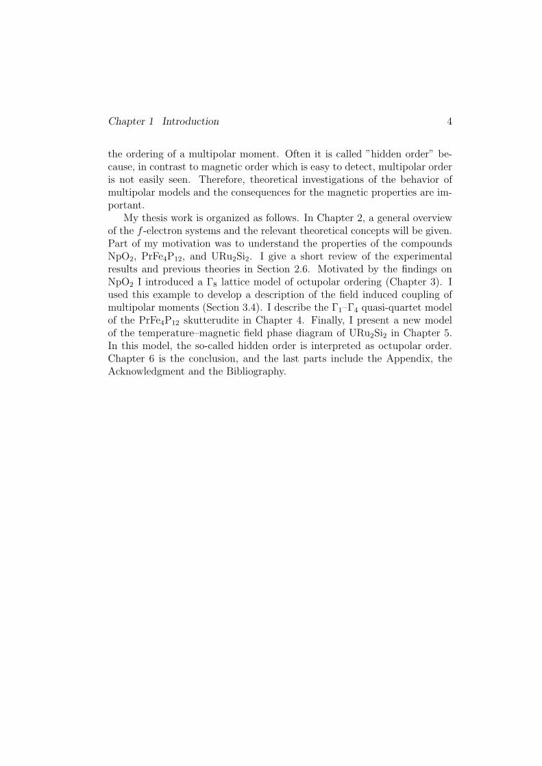
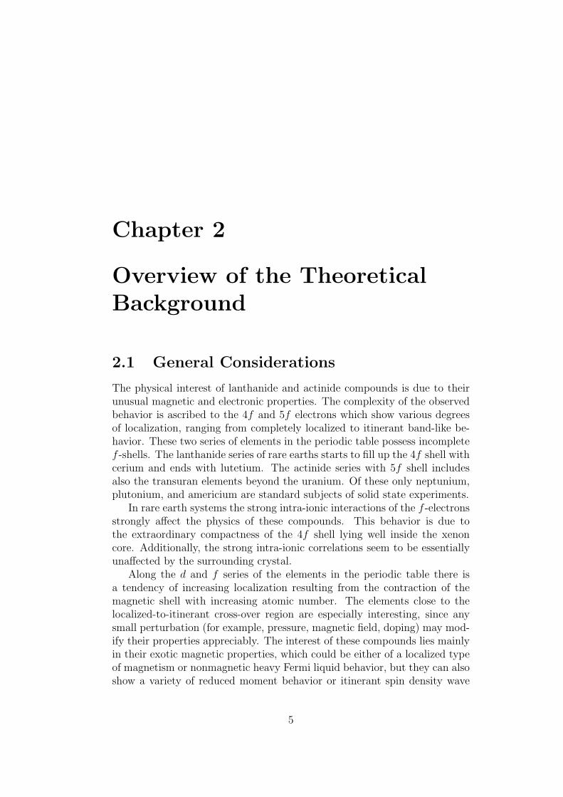
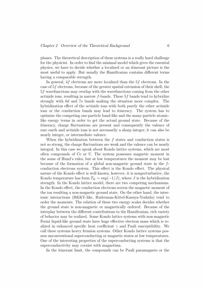

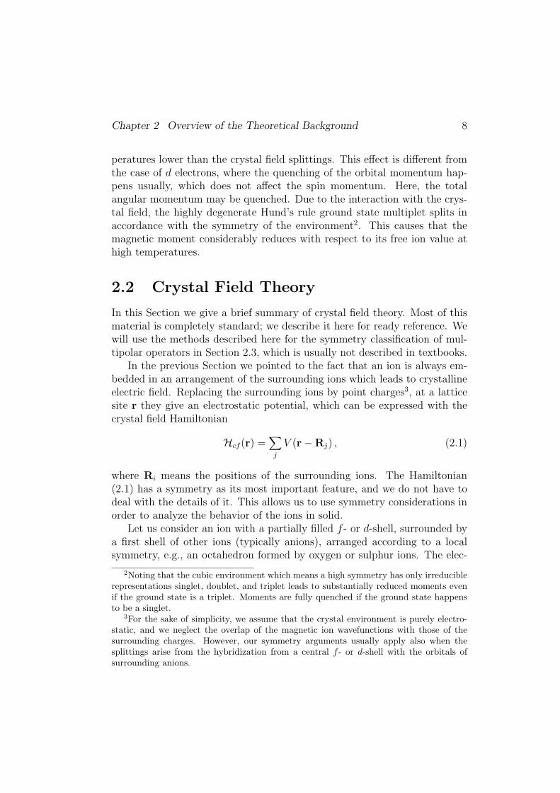
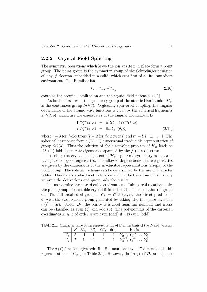
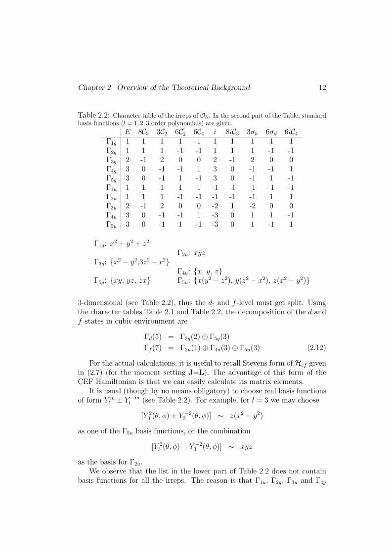
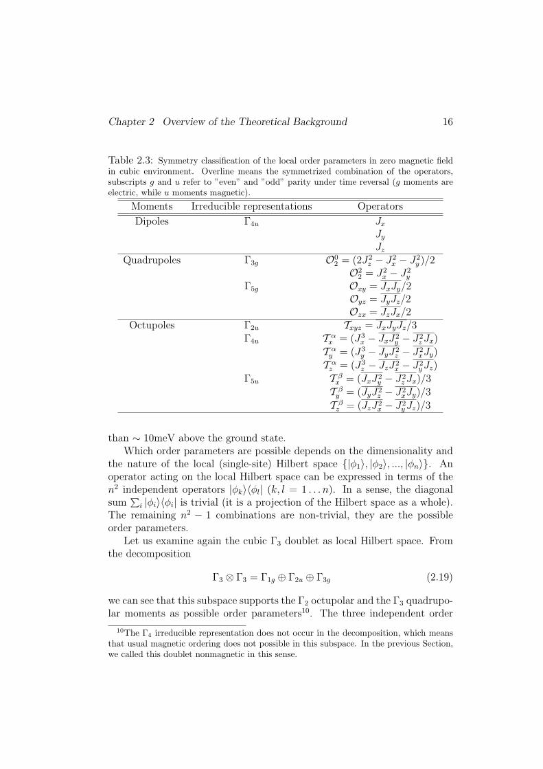
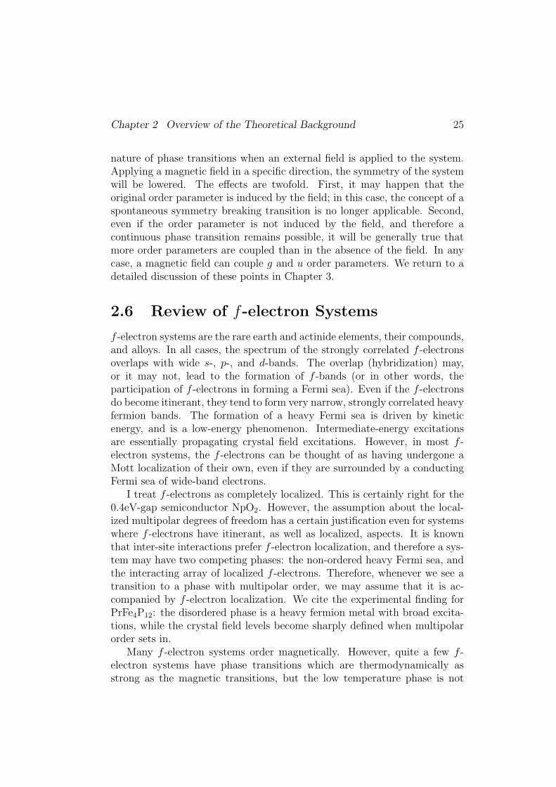
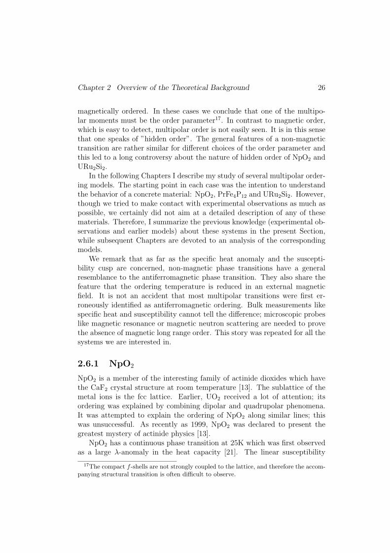
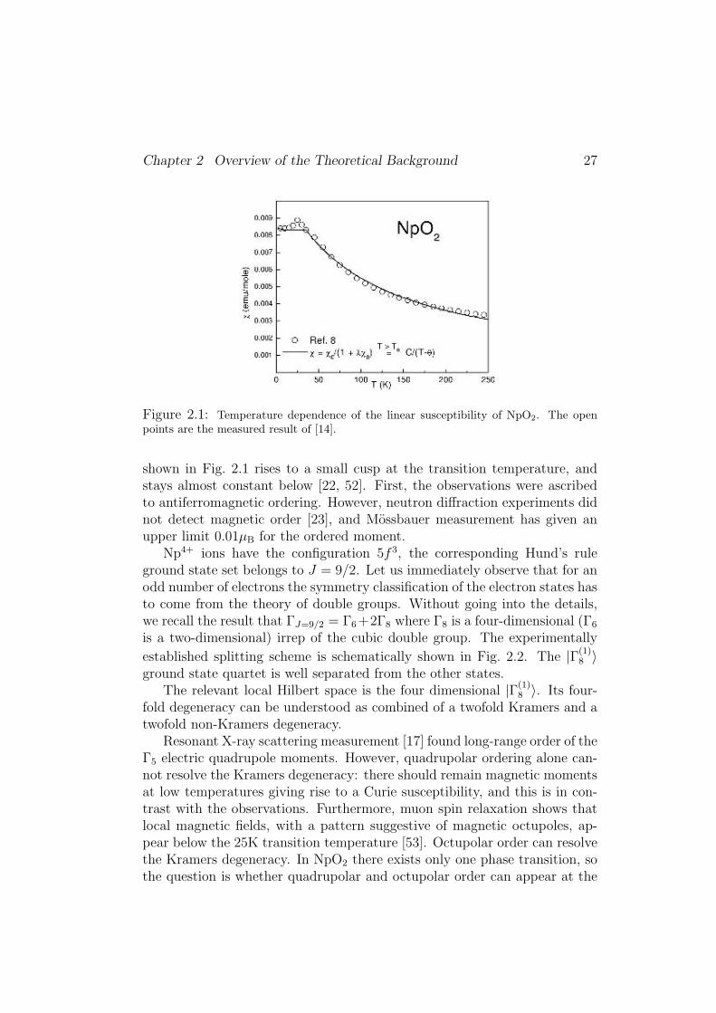
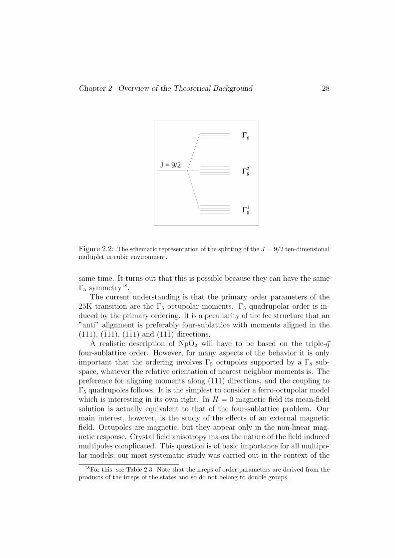
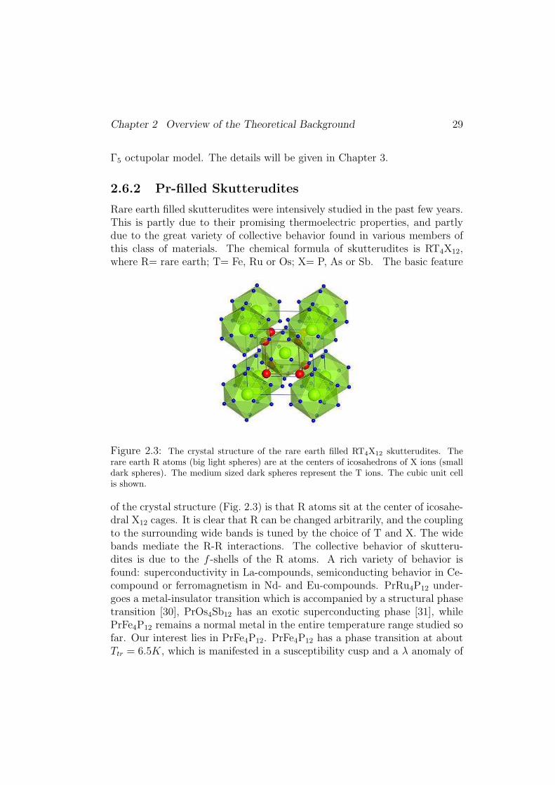
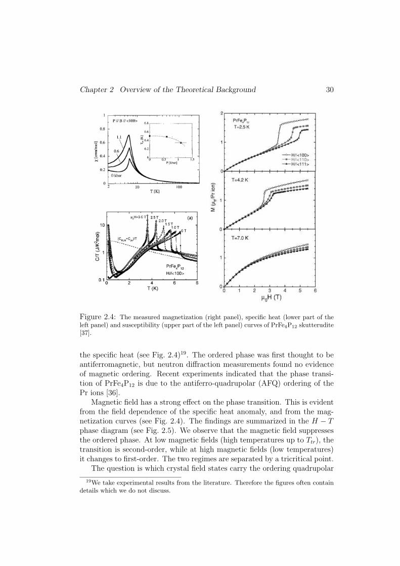
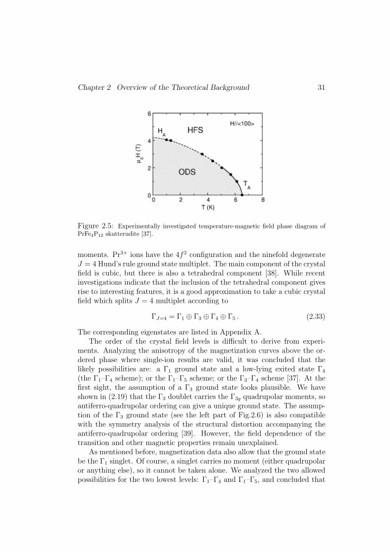
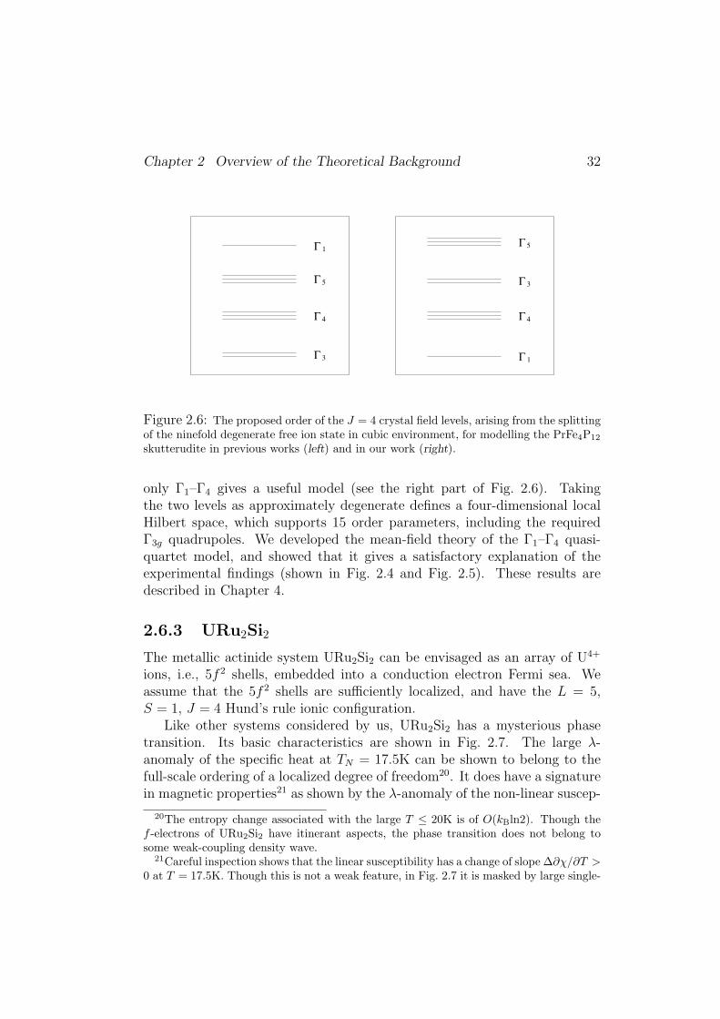
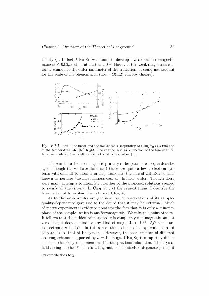
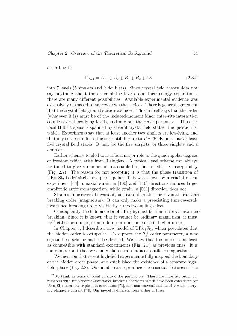
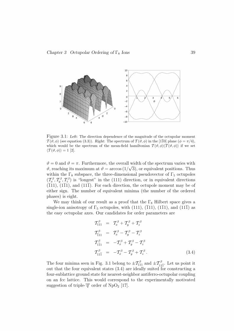
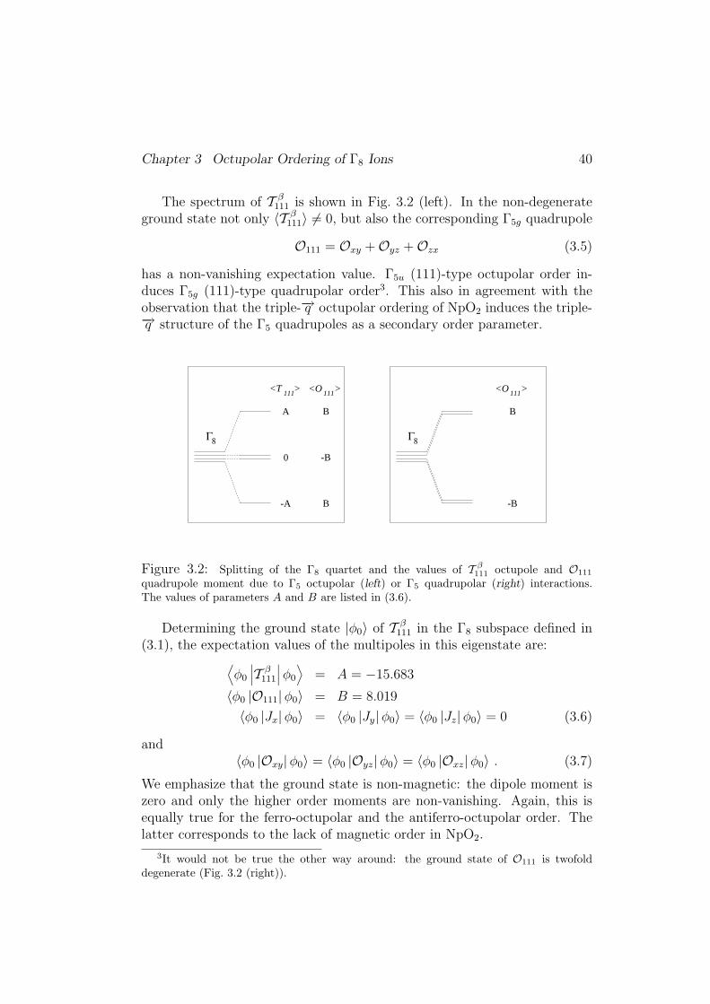
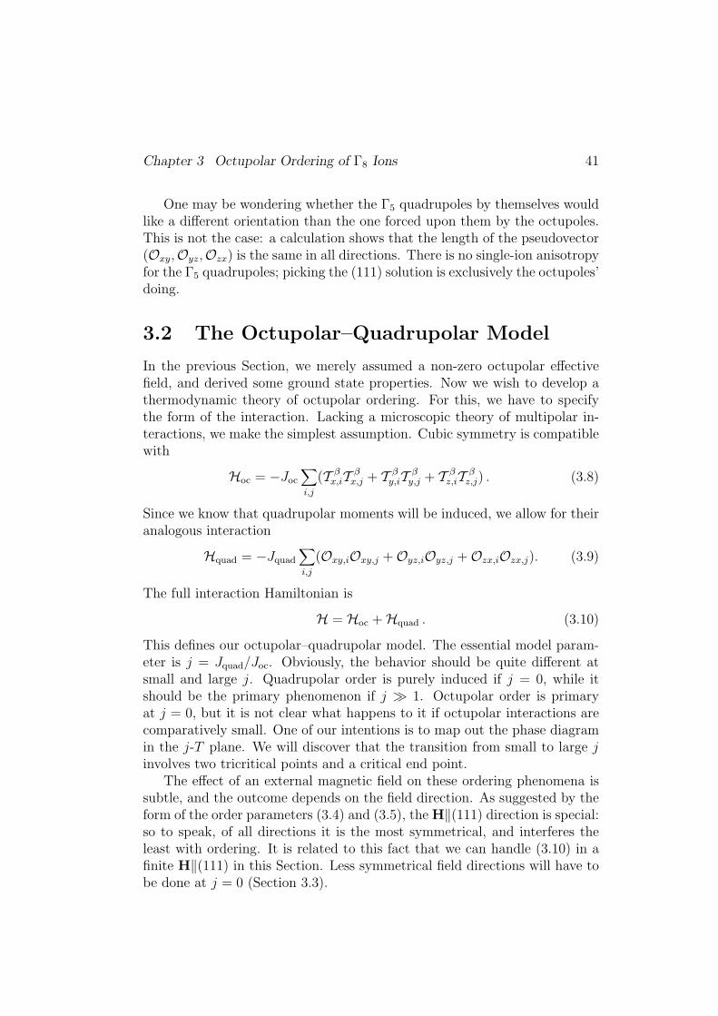
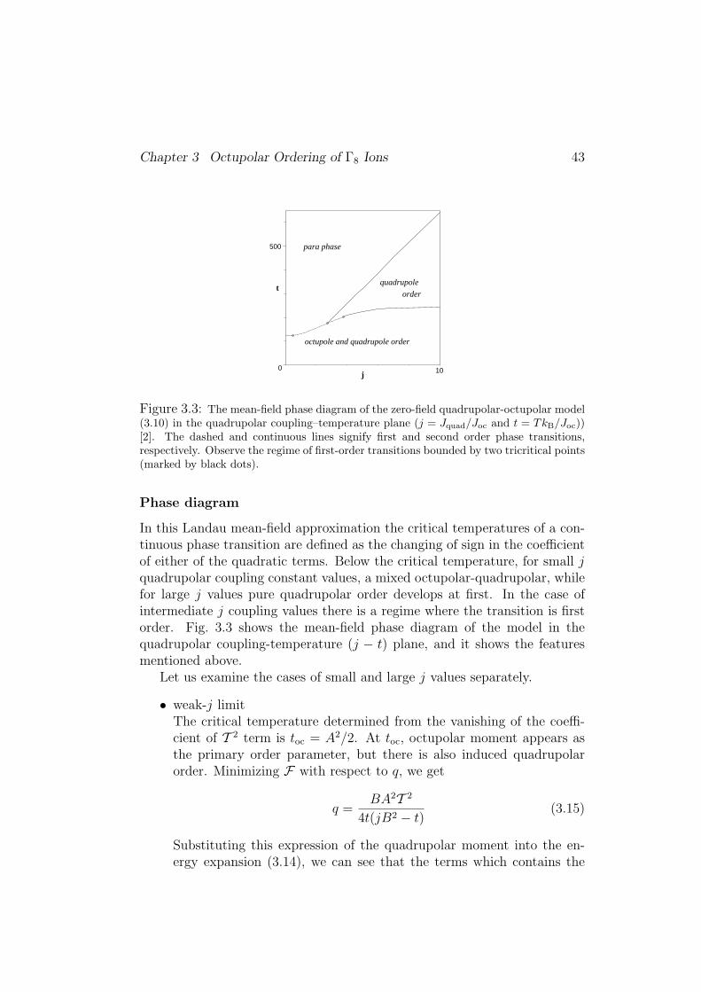
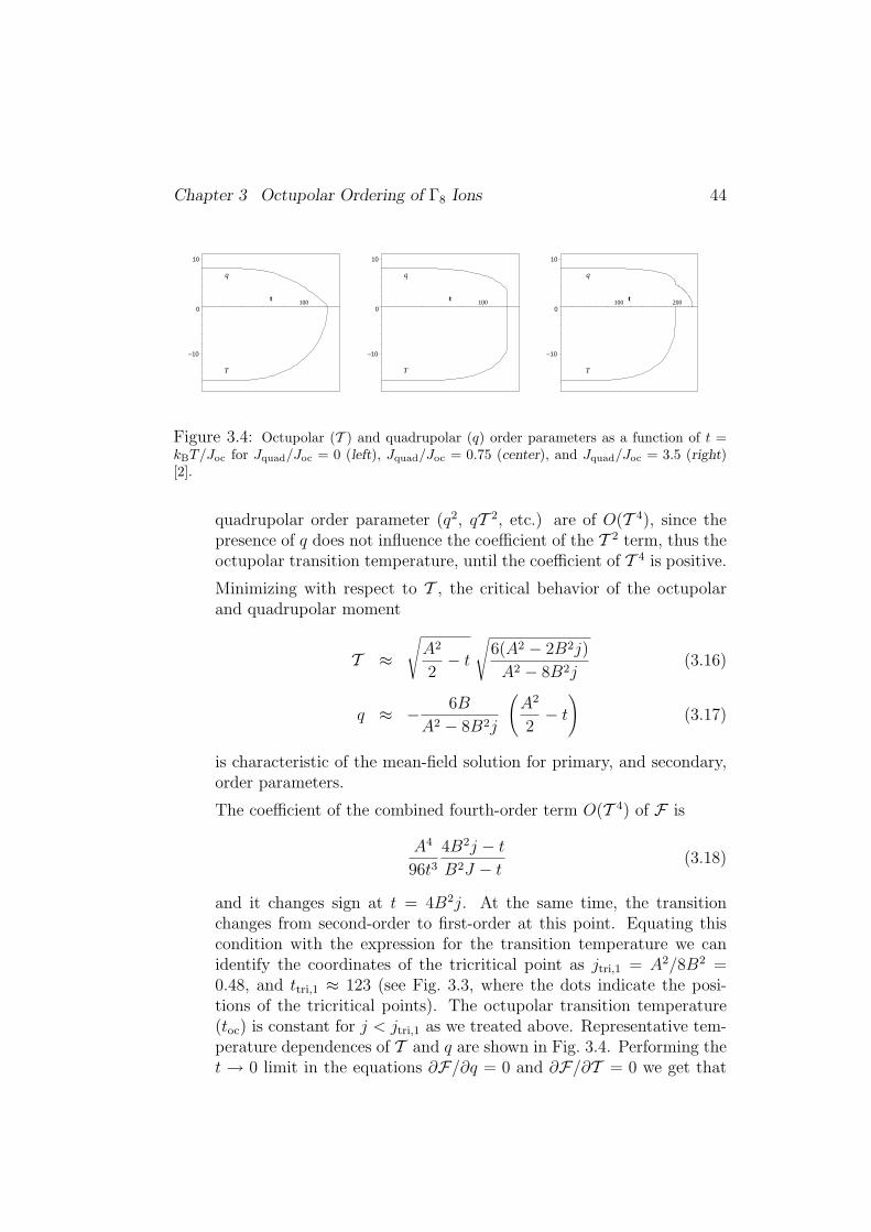
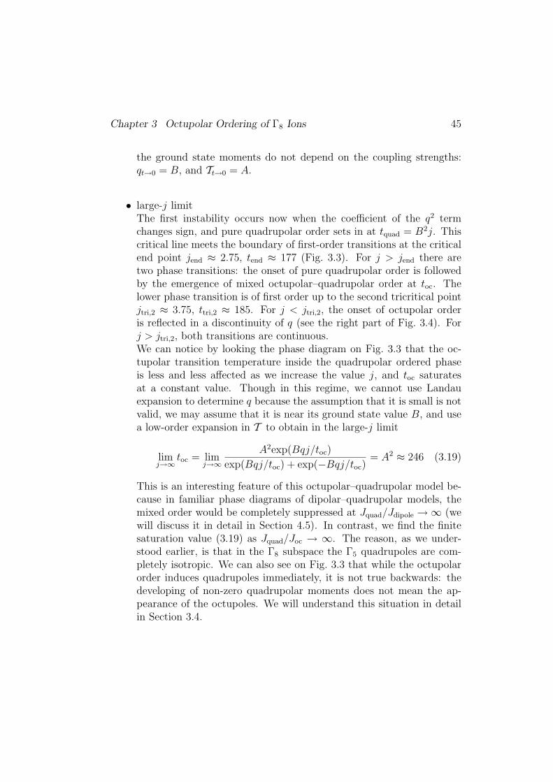
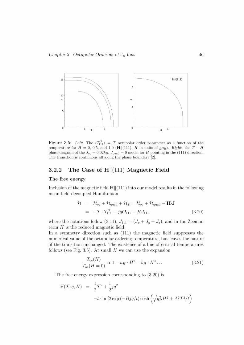
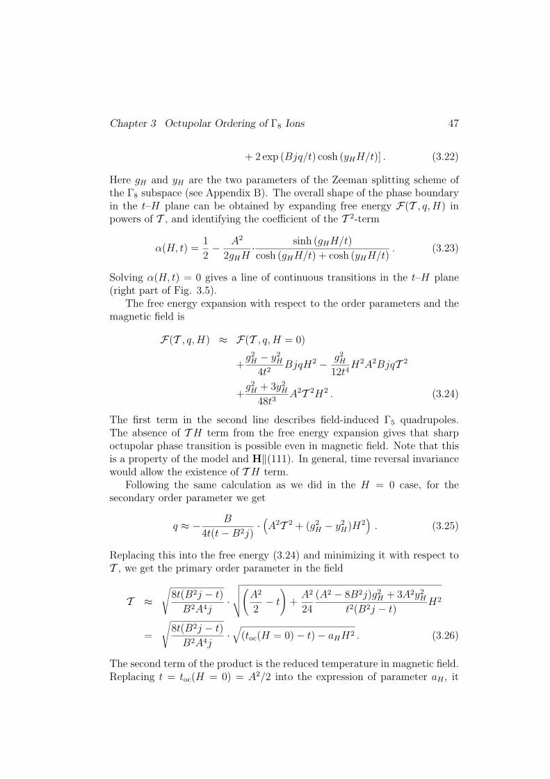
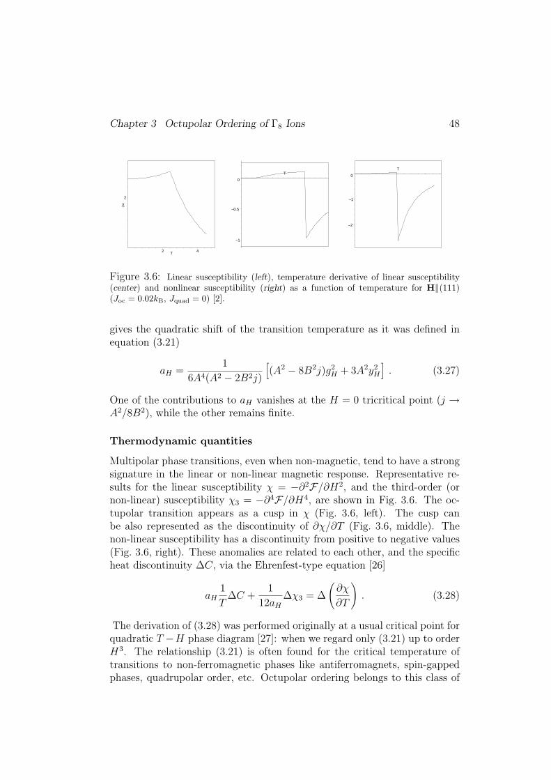
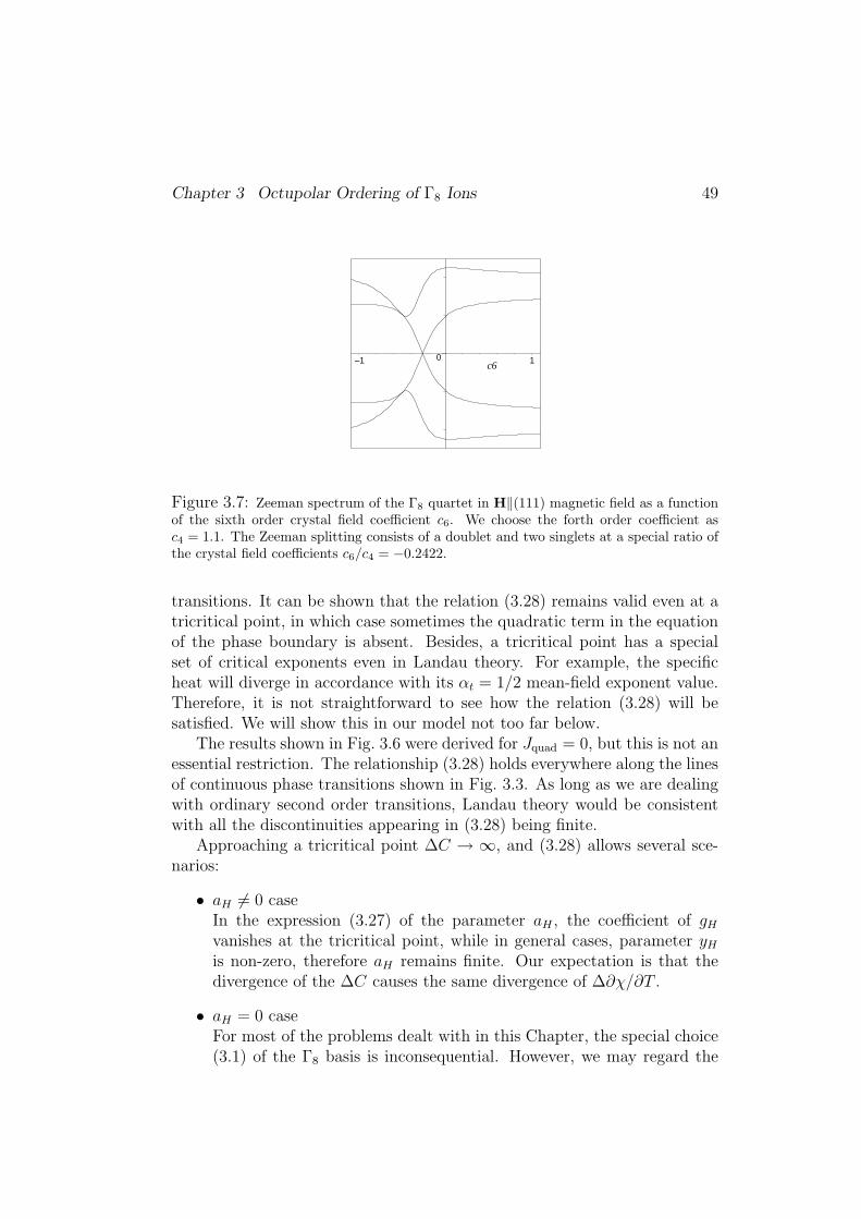

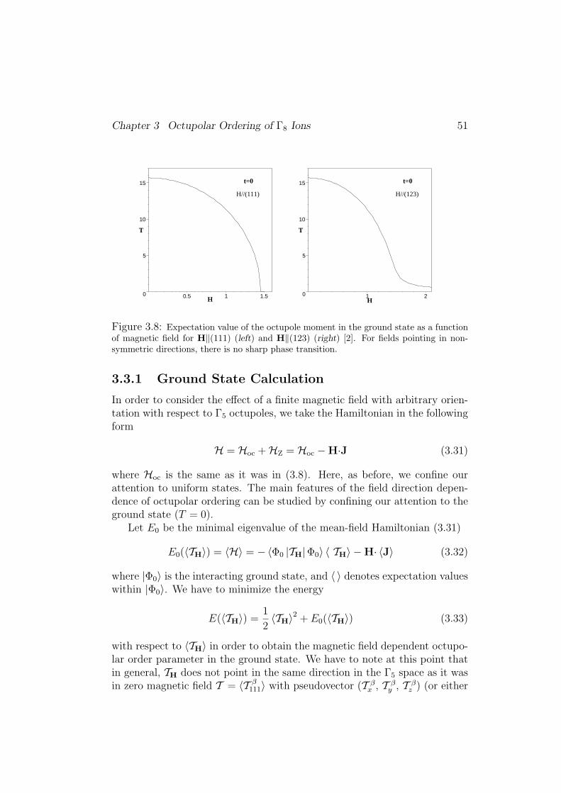
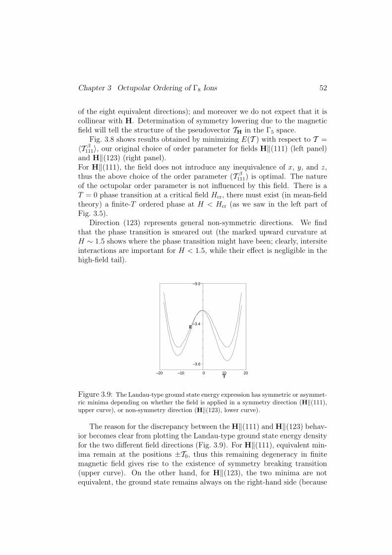
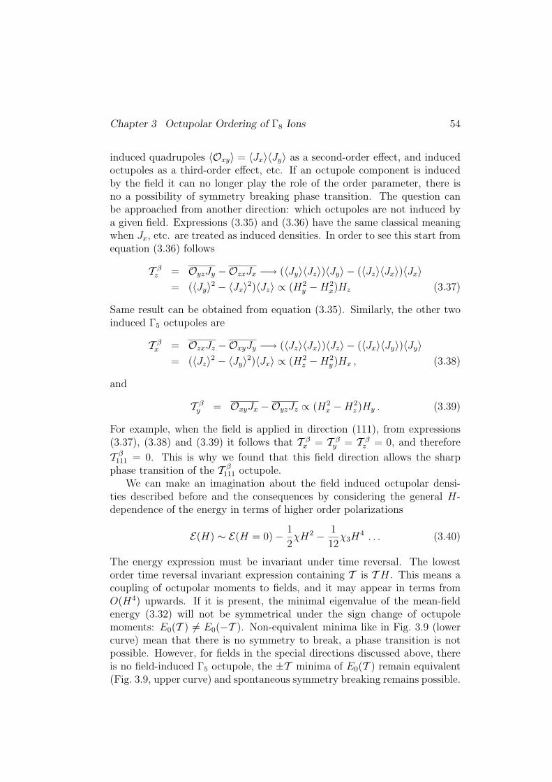
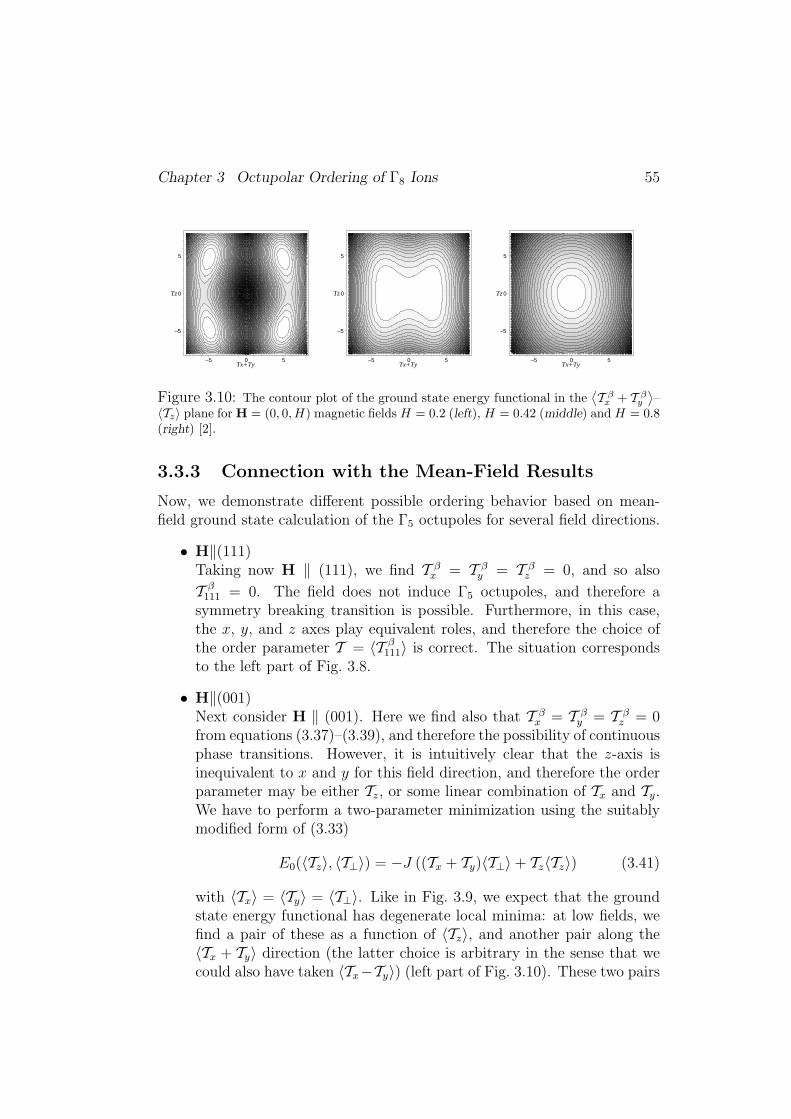
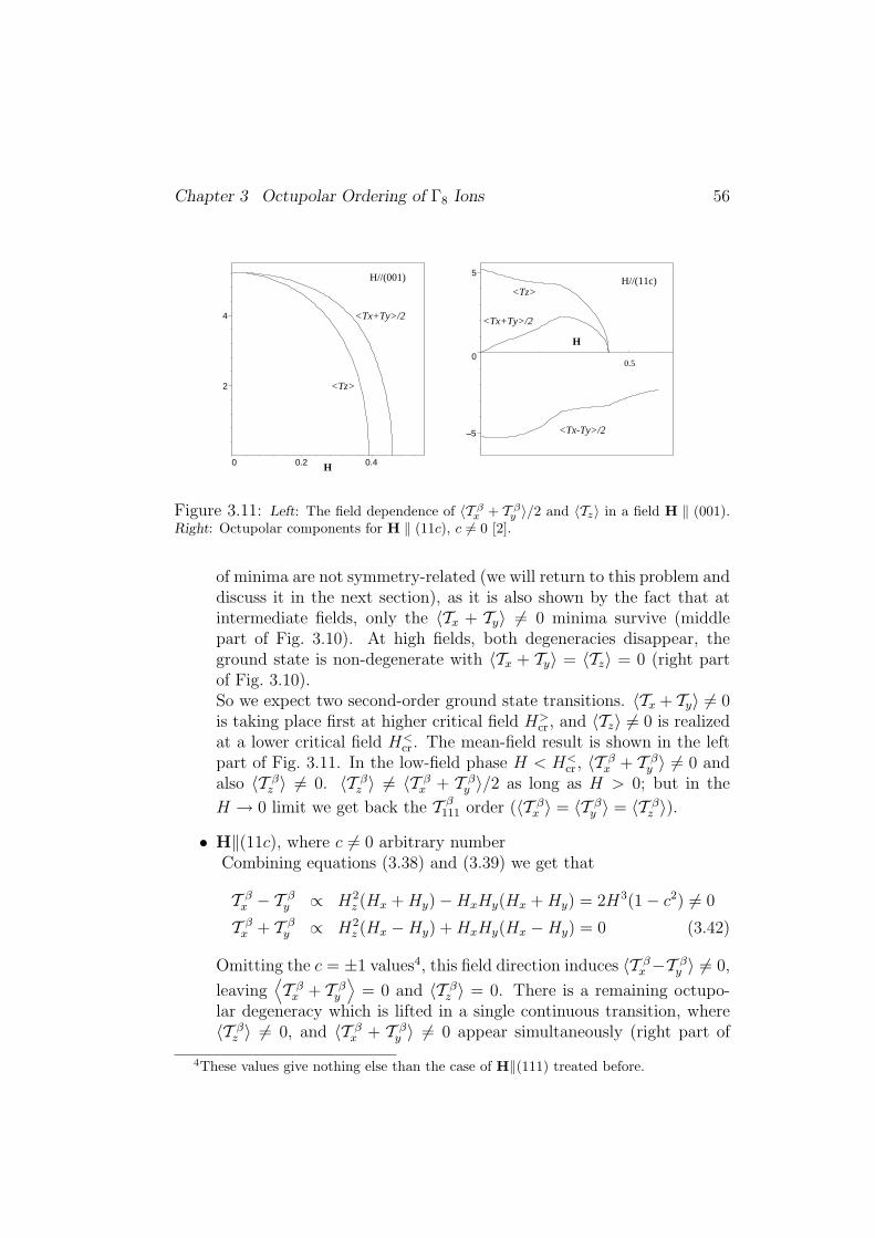

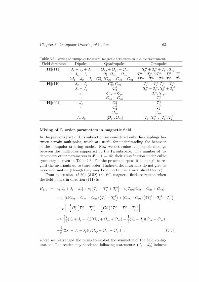
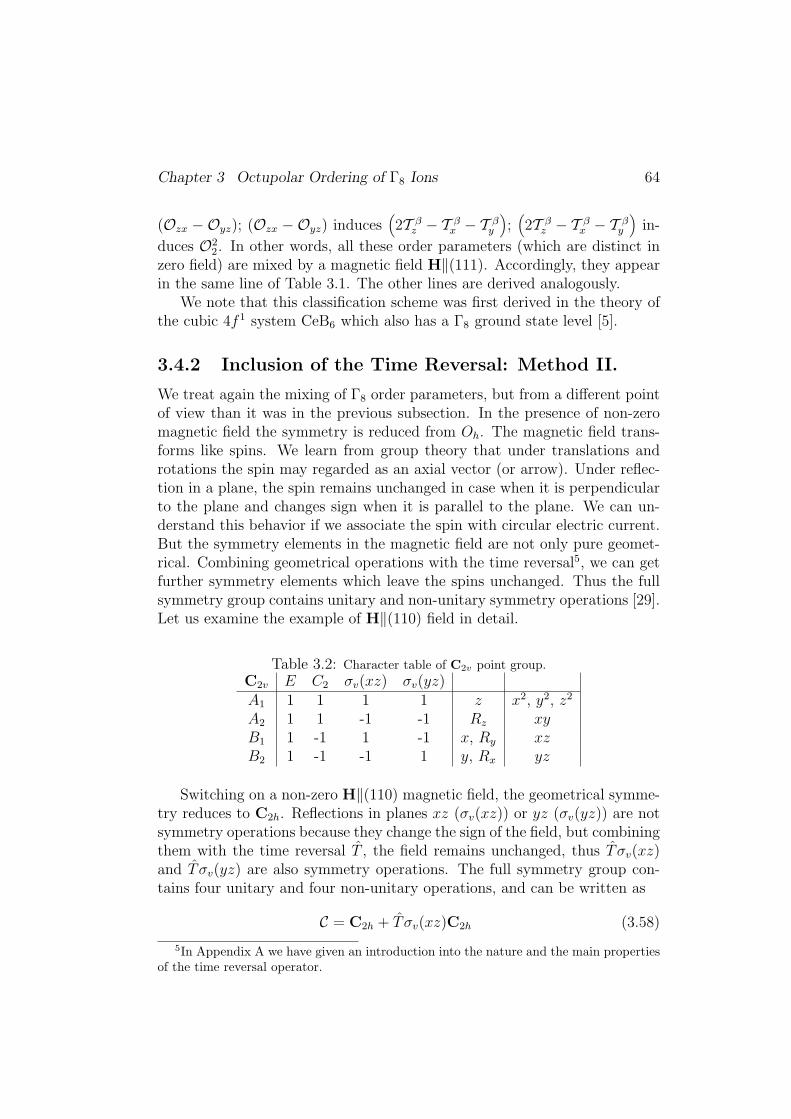
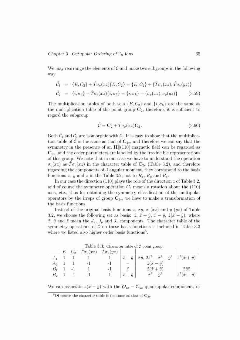
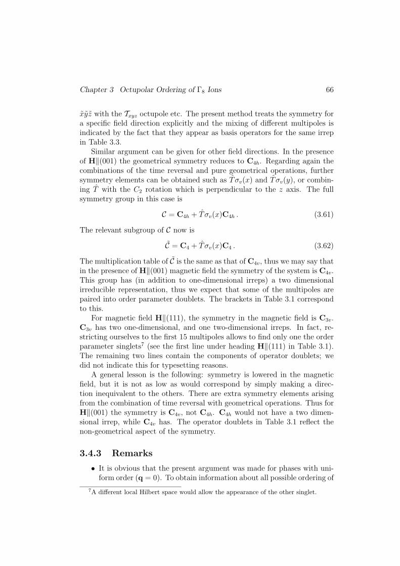
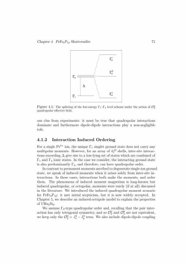
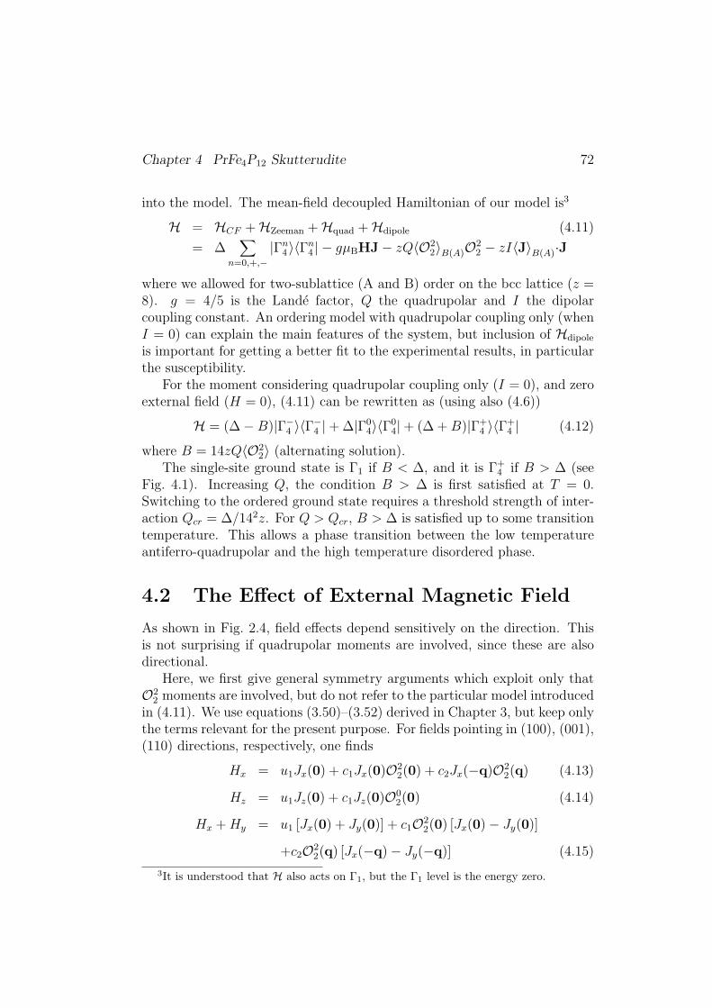
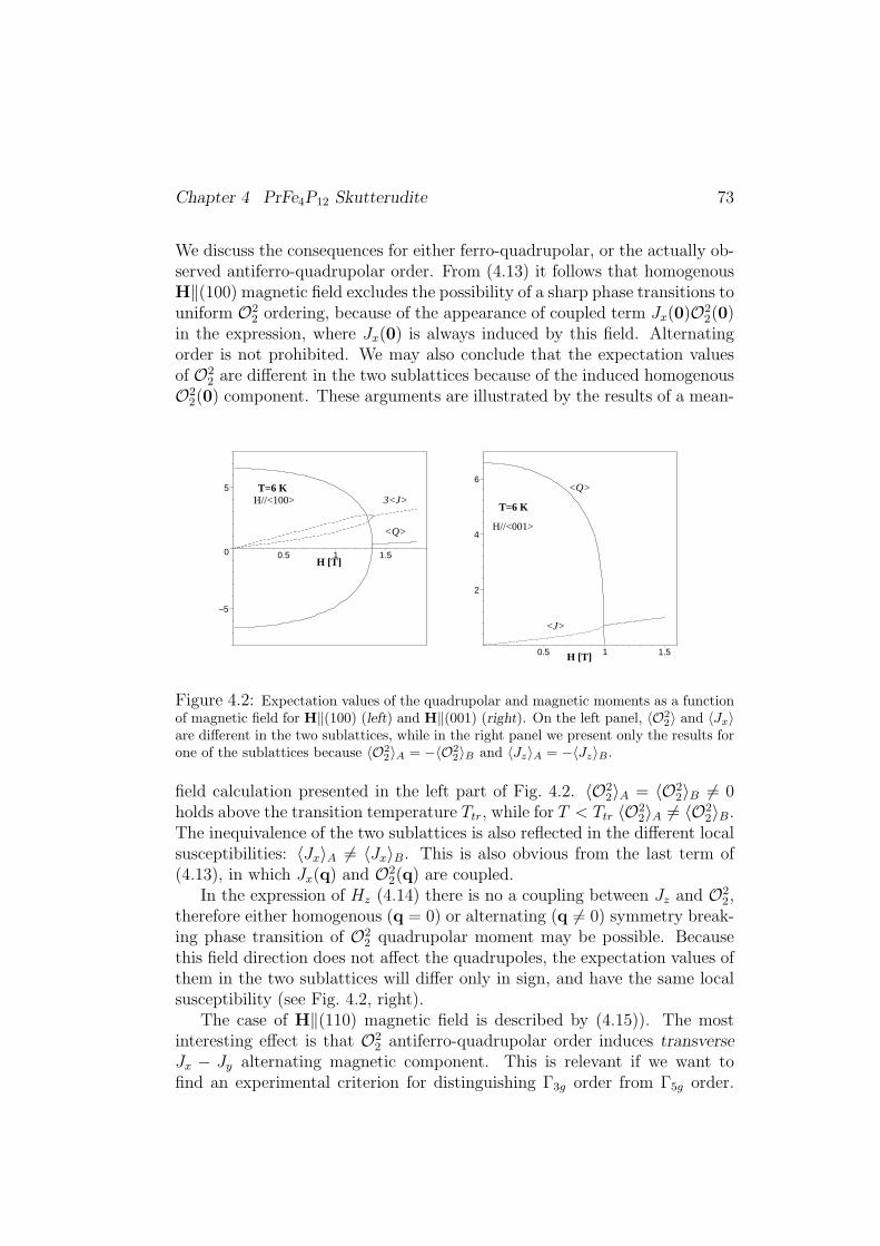
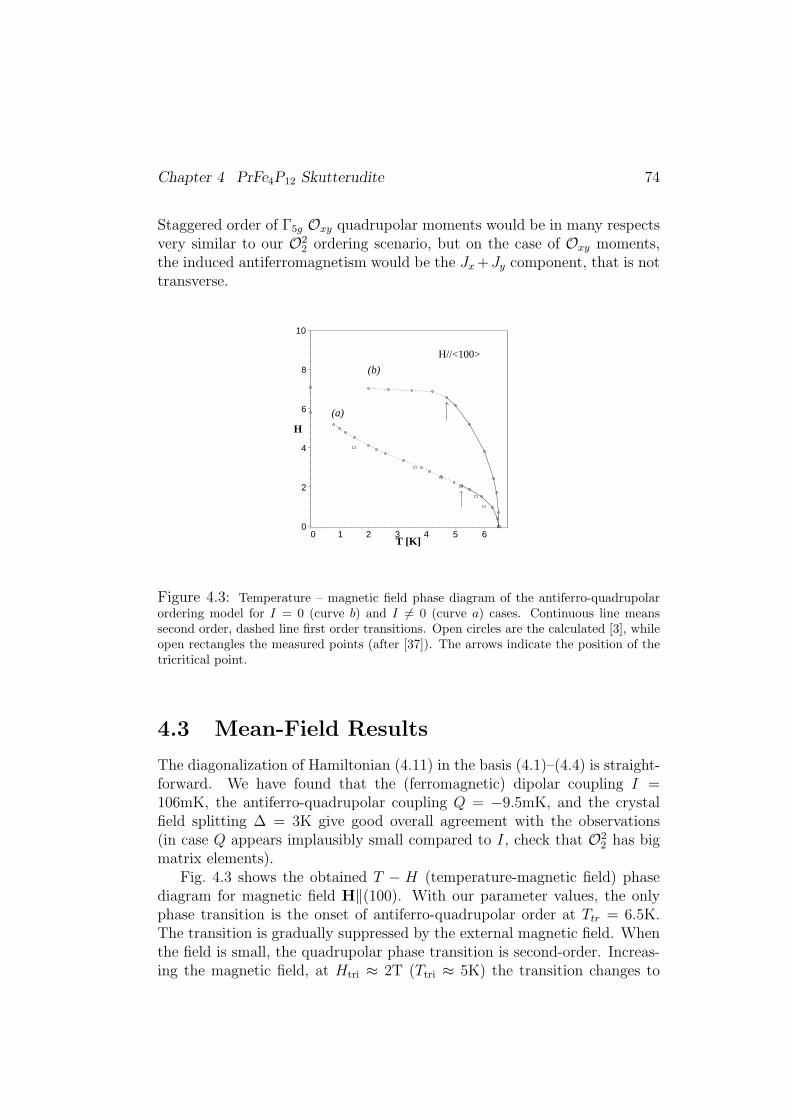
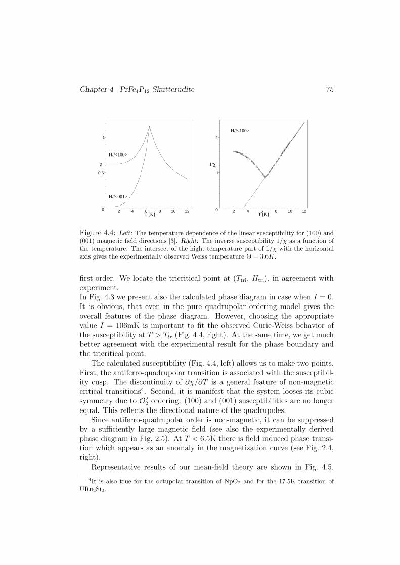
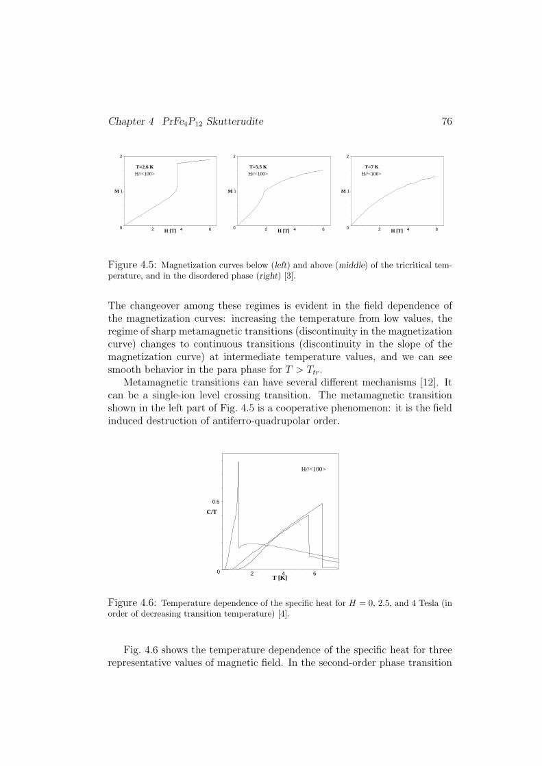
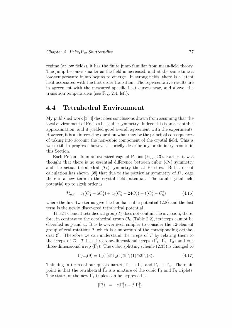
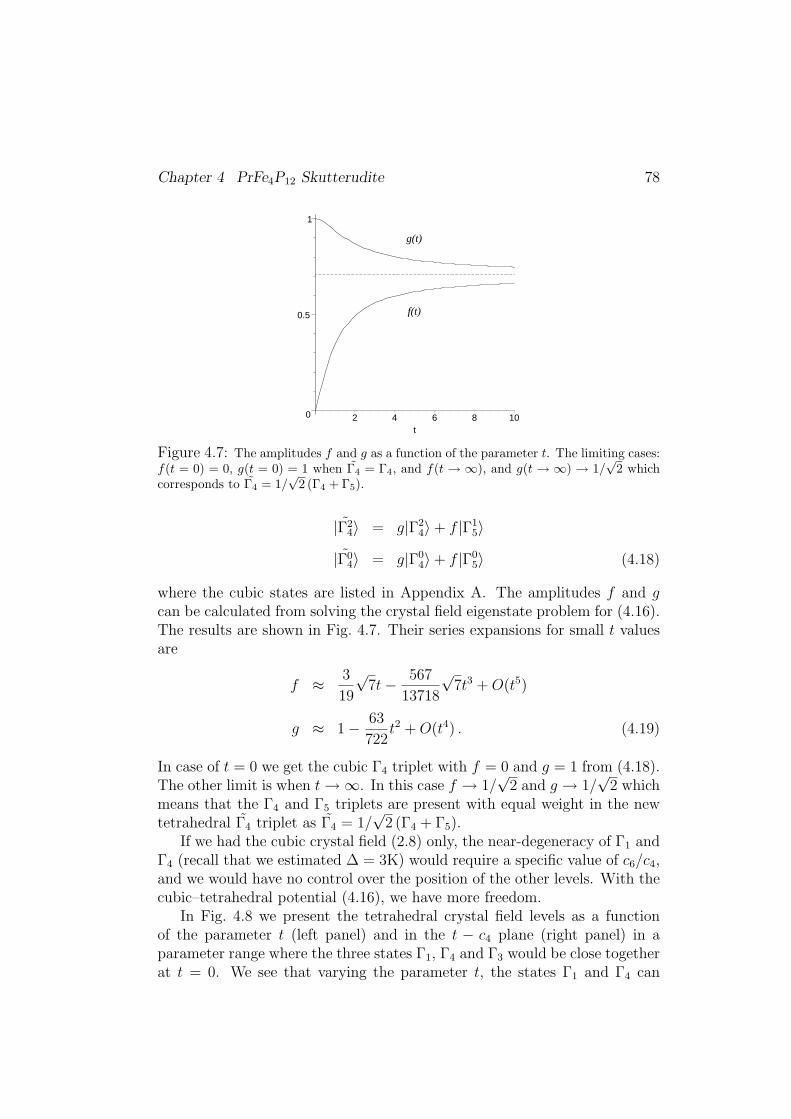
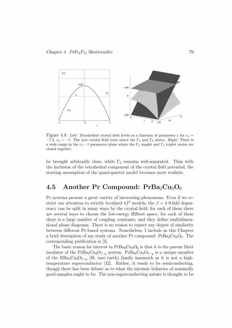
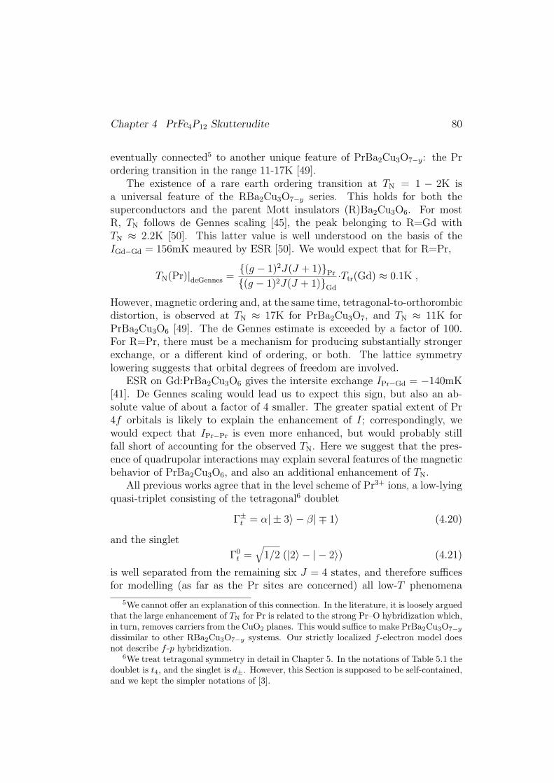
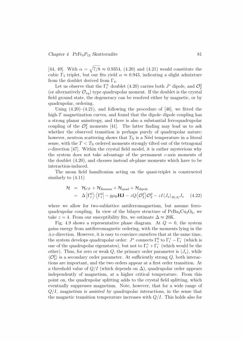
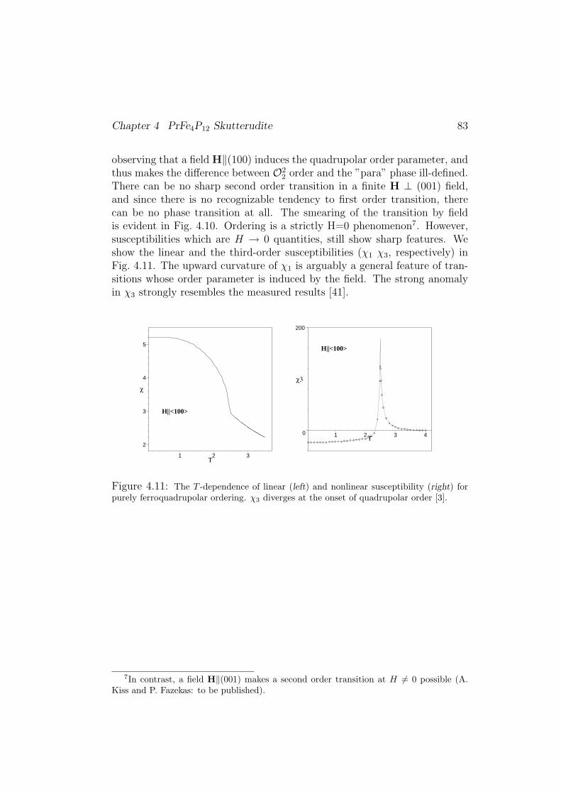


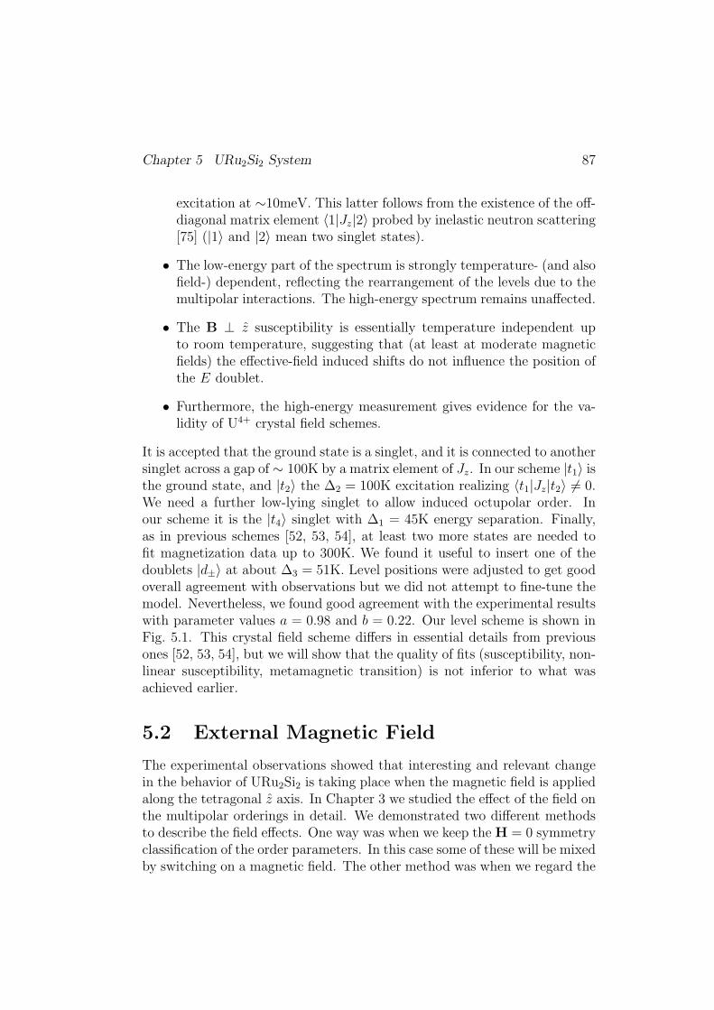
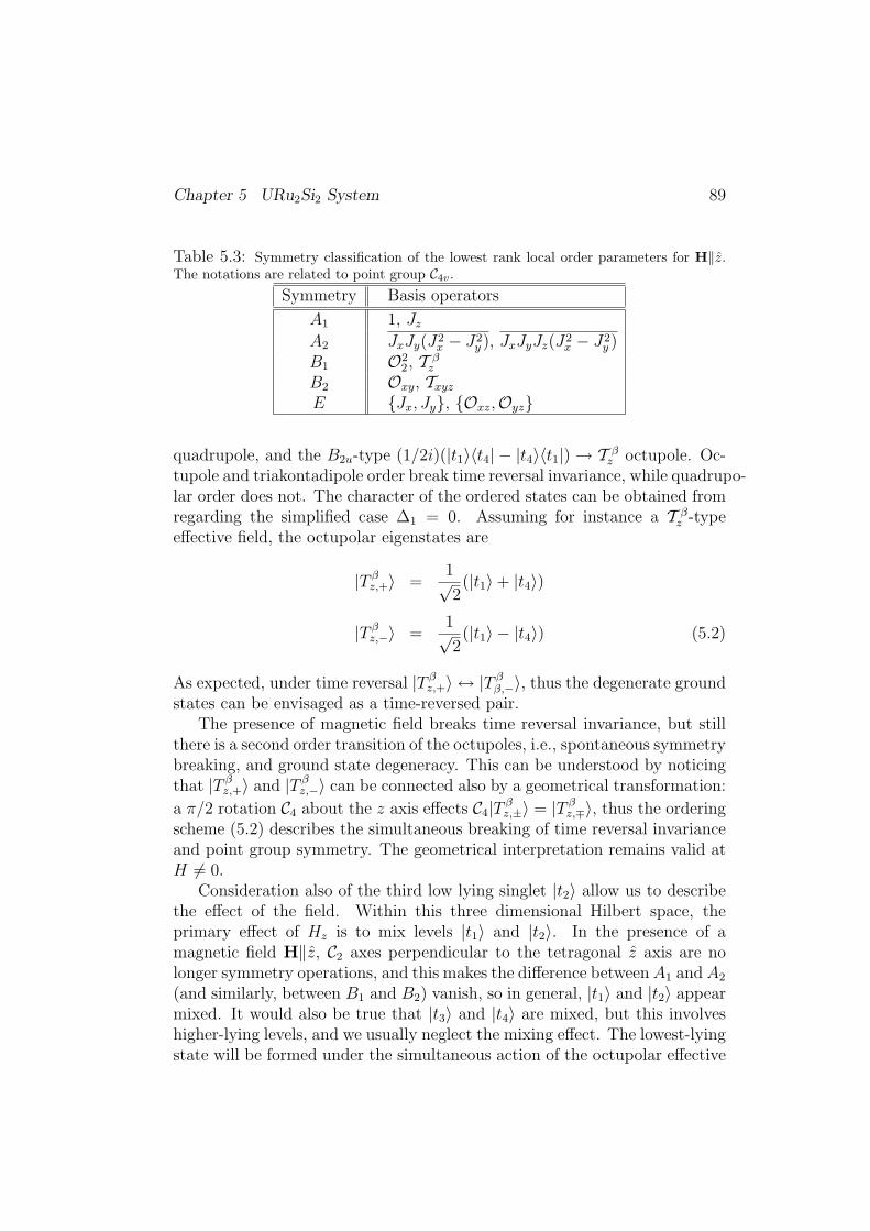
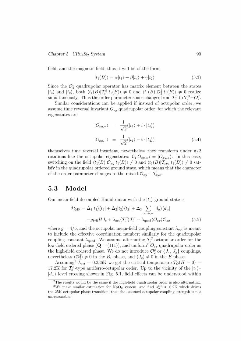
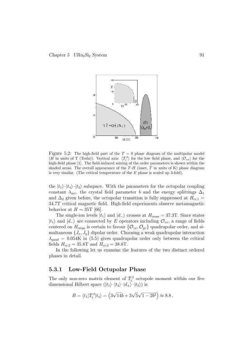
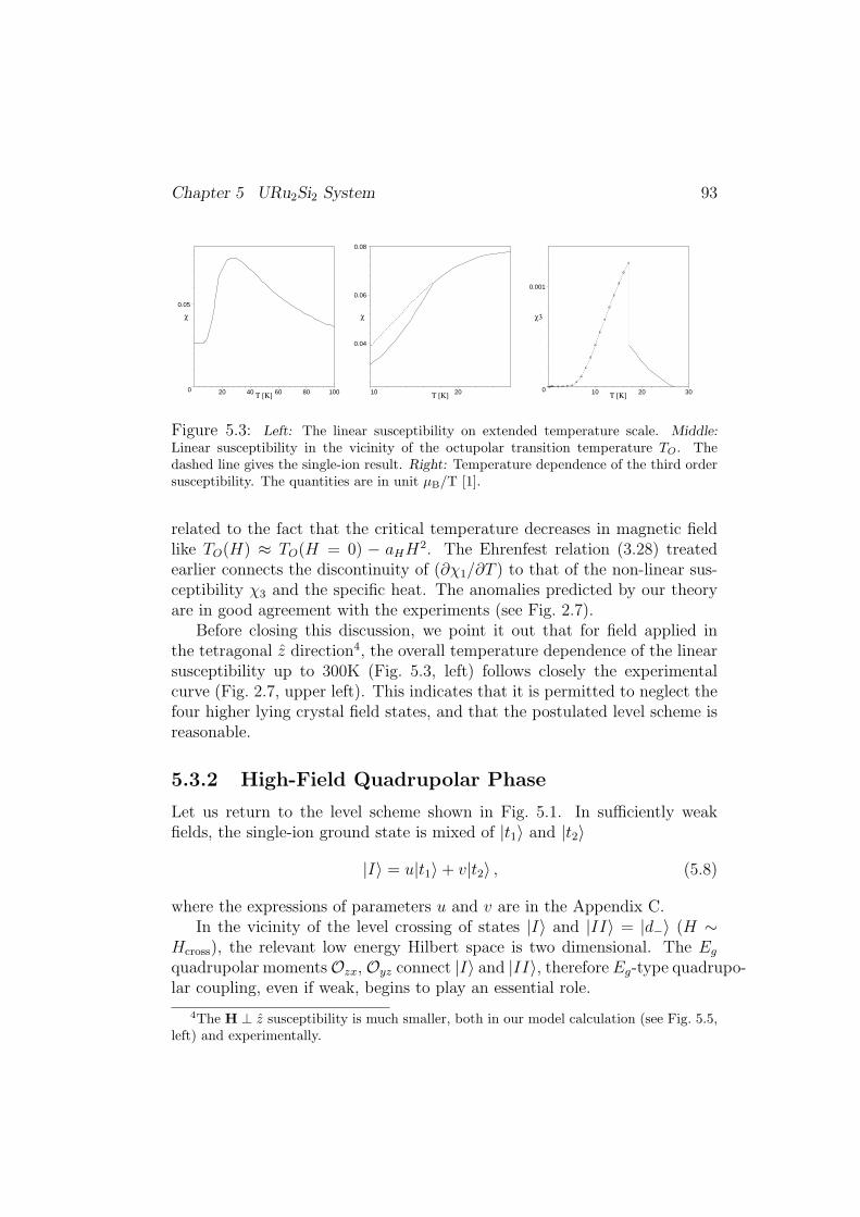
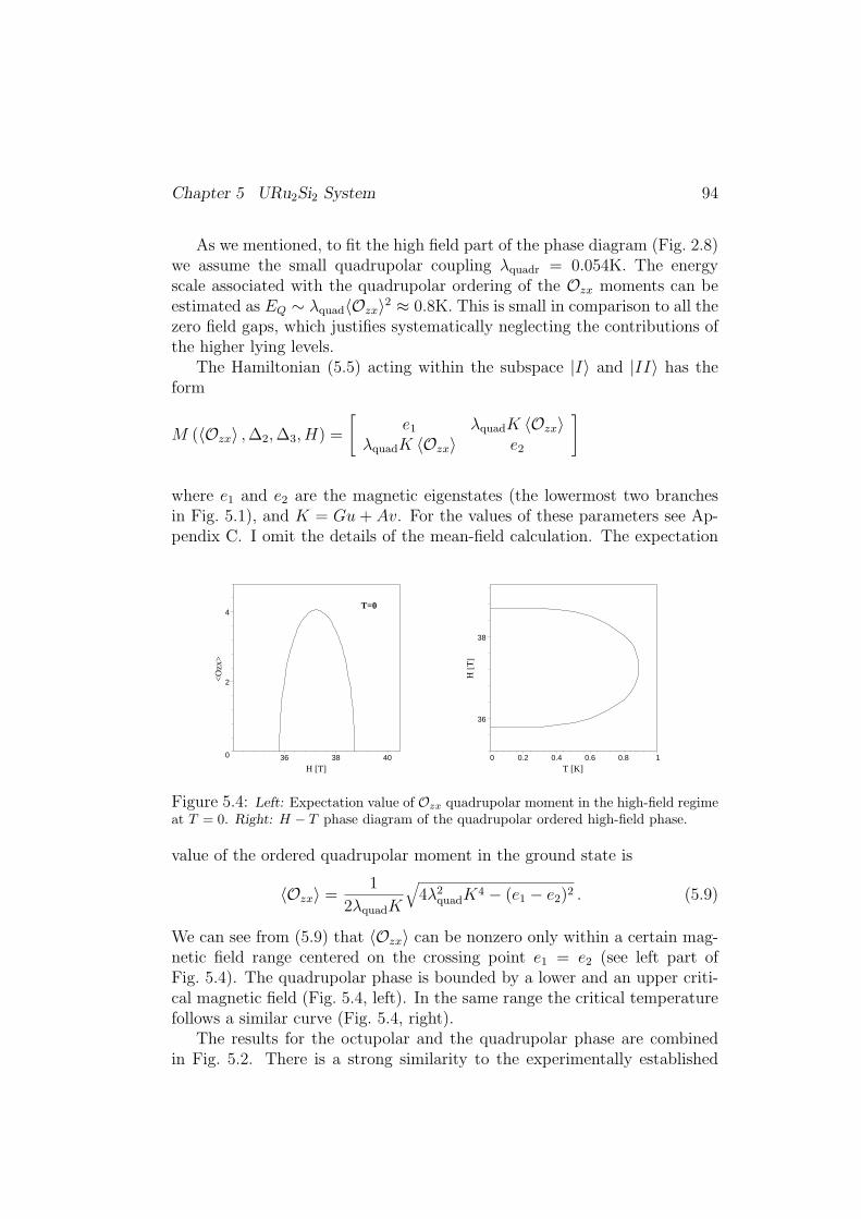
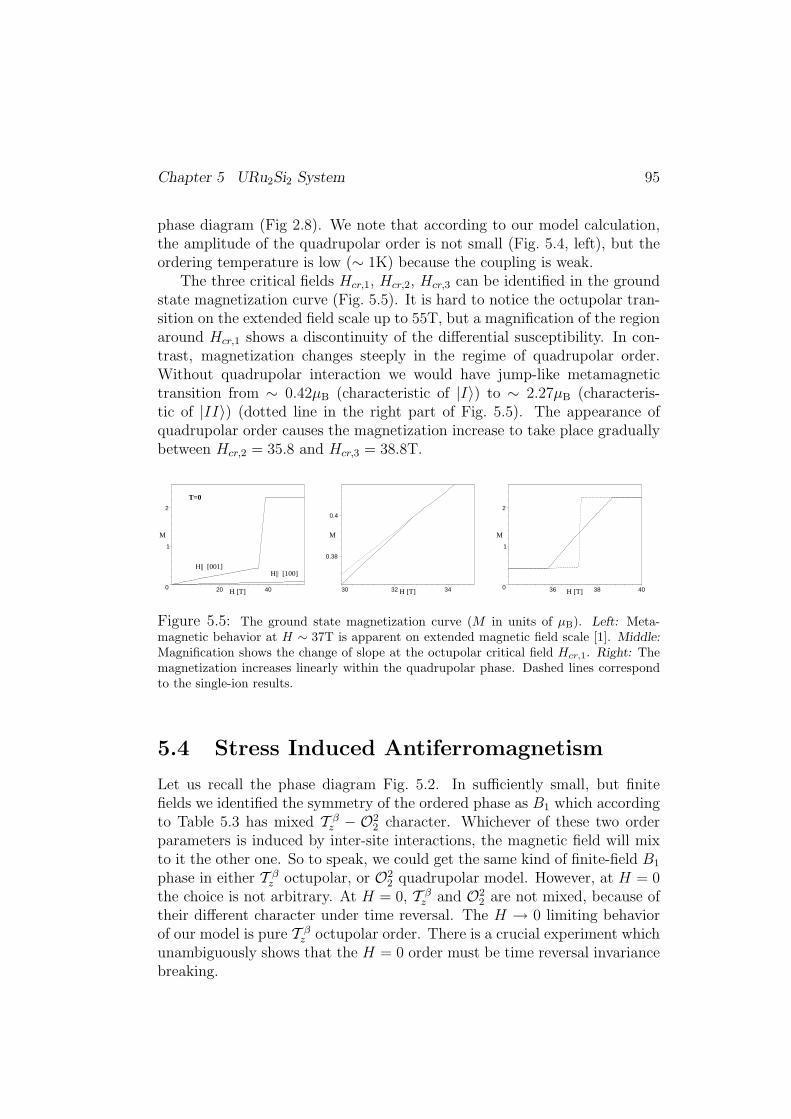
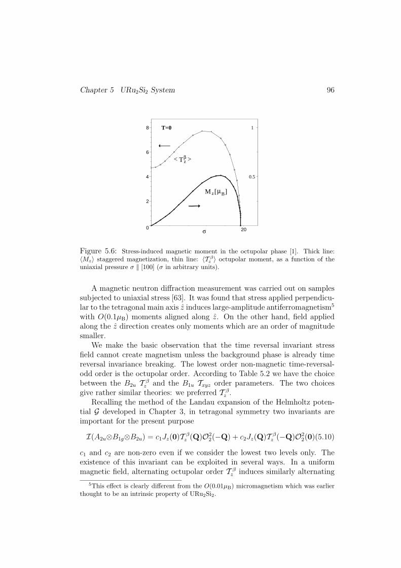


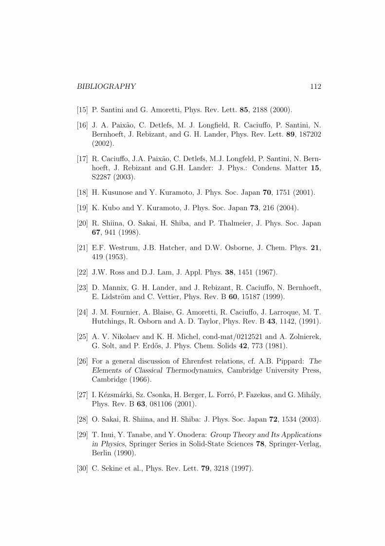
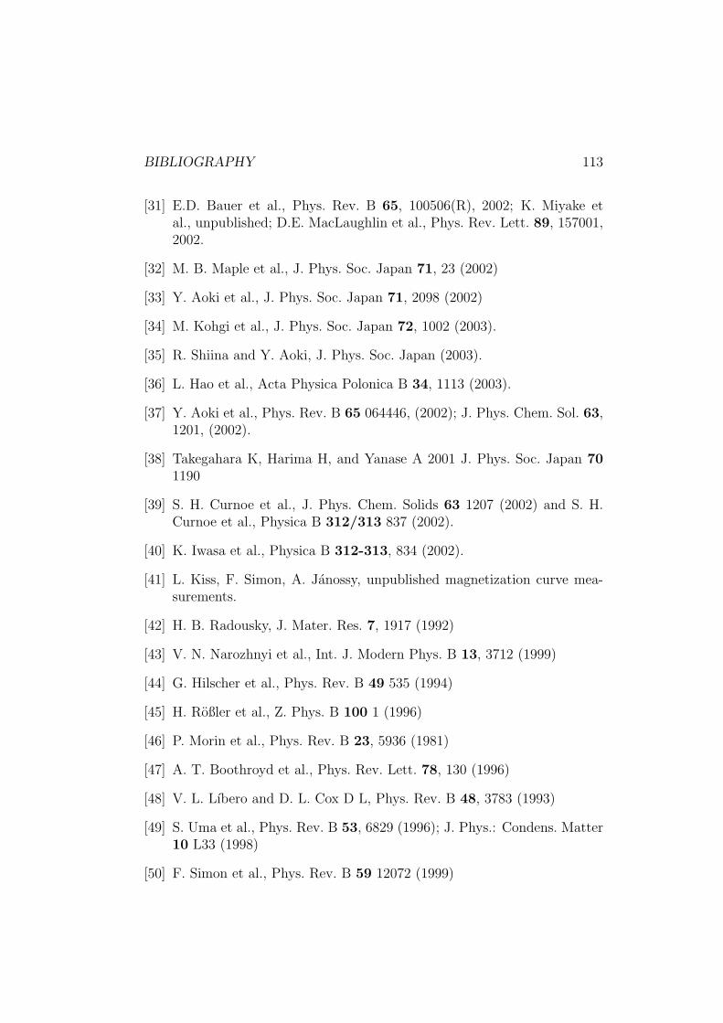
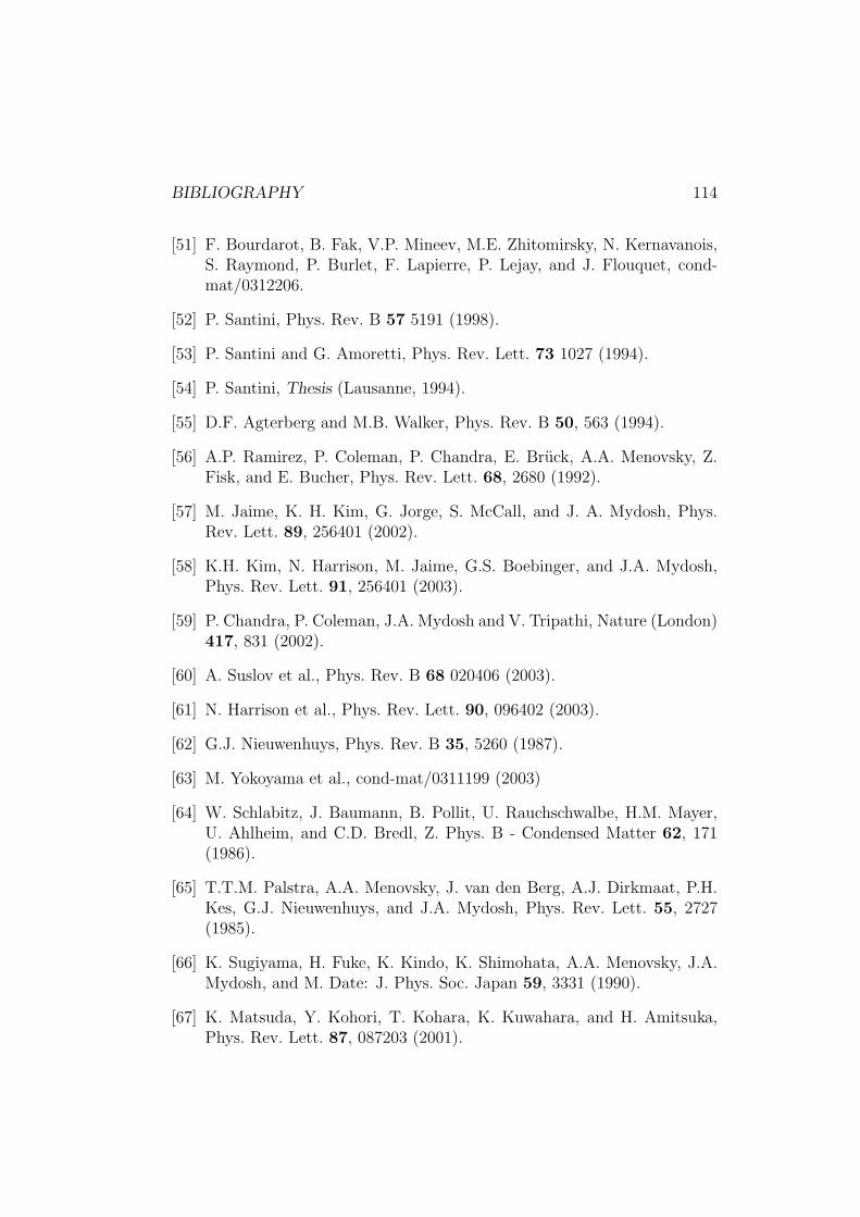


![Two-stage multipolar ordering in PrT2Al20 Kondo materials€¦ · [2–5,35]. The transition between these phases might be driven by increasing pressure or by choice of the T ion;](https://static.documents.pub/doc/80x56/5f916191574a7c792f76c181/two-stage-multipolar-ordering-in-prt2al20-kondo-2a535-the-transition-between.jpg)


