Phenomenological many‐body potentials from the interstitial electron model. I. Dynamic properties of metals Mo Li and William A. Goddard III Citation: The Journal of Chemical Physics 98, 7995 (1993); doi: 10.1063/1.464553 View online: http://dx.doi.org/10.1063/1.464553 View Table of Contents: http://scitation.aip.org/content/aip/journal/jcp/98/10?ver=pdfcov Published by the AIP Publishing Articles you may be interested in On the problem of fitting many-body potentials. I. The minimal maximum error scheme and the paradigm of metal systems J. Chem. Phys. 110, 8899 (1999); 10.1063/1.478809 Molecular dynamics study of the Ag 6 cluster using an ab initio many-body model potential J. Chem. Phys. 109, 2176 (1998); 10.1063/1.476851 Modeling calcium and strontium clusters with many-body potentials J. Chem. Phys. 107, 4674 (1997); 10.1063/1.474829 A many‐body confinement potential model for multi‐hadron systems AIP Conf. Proc. 110, 100 (1984); 10.1063/1.34343 The electronic structure of molecules by a many‐body approach. I. Ionization potentials and one‐electron properties of benzene J. Chem. Phys. 65, 1378 (1976); 10.1063/1.433244 This article is copyrighted as indicated in the article. Reuse of AIP content is subject to the terms at: http://scitation.aip.org/termsconditions. Downloaded to IP: 131.215.70.231 On: Mon, 04 Jan 2016 19:13:08
Transcript
Phenomenological many‐body potentials from the interstitial electron model. I.Dynamic properties of metalsMo Li and William A. Goddard III Citation: The Journal of Chemical Physics 98, 7995 (1993); doi: 10.1063/1.464553 View online: http://dx.doi.org/10.1063/1.464553 View Table of Contents: http://scitation.aip.org/content/aip/journal/jcp/98/10?ver=pdfcov Published by the AIP Publishing Articles you may be interested in On the problem of fitting many-body potentials. I. The minimal maximum error scheme and the paradigm ofmetal systems J. Chem. Phys. 110, 8899 (1999); 10.1063/1.478809 Molecular dynamics study of the Ag 6 cluster using an ab initio many-body model potential J. Chem. Phys. 109, 2176 (1998); 10.1063/1.476851 Modeling calcium and strontium clusters with many-body potentials J. Chem. Phys. 107, 4674 (1997); 10.1063/1.474829 A many‐body confinement potential model for multi‐hadron systems AIP Conf. Proc. 110, 100 (1984); 10.1063/1.34343 The electronic structure of molecules by a many‐body approach. I. Ionization potentials and one‐electronproperties of benzene J. Chem. Phys. 65, 1378 (1976); 10.1063/1.433244
This article is copyrighted as indicated in the article. Reuse of AIP content is subject to the terms at: http://scitation.aip.org/termsconditions. Downloaded to IP:
Phenomenological many-body potentials from the interstitial electron model. I. Dynamic properties of metals
Mo Ua) and William A. Goddard IlIb),c)
California Institute of Technology, Pasadena, California 91125 d)
(Received 6 November 1992; accepted 28 January 1993)
Inspired by the ab initio generalized-valence-bond calculations of small metal clusters, we propose a phenomenological many-body interaction model, the interstitial electron model (IEM), for interactions of ions and electrons in metals. In this model, the valence electrons are treated as classical particles situated at the crystal lattice interstitial positions. Simple pair potentials are used for ions and interstitial electrons, allowing the inhomogeneity and anisotropy of electron density distributions to be taken into account phenomenologically. To test the efficacy and applicability of this approach, the IEM is applied to lattice dynamics in fcc metals: Cu, Ni, Ag, Au, Pd, Pt, AI, Ca, Sr, and y-Fe. The phonon dispersion relations, densities of states, and Debye temperature are calculated and found to be in good agreement with experiments. Extension of the IEM to the construction of a new many-body potential in metals and alloys is discussed.
I. INTRODUCTION
Although pairwise interatomic interactions are still widely used in theories and simulations of condensed matter, much attention has been paid to incorporating manybody electron effects into an empirical interatomic potential. 1 More specifically, the handling of the inhomogeneity and anisotropy in the electron density distribution is the center of interest. The simplest approach is to add to the pair potentiae,3 a crystal volume dependent energy term which arises mainly from the density dependent electron kinetic energy. However, the introduction of such a volume dependent energy, or homogeneous electron density dependent energy, usually leads to the so called compressibility paradox: the compressibility derived from the long wave limit is not the same as that derived from homogeneous deformation. Moreover, the volume dependent pair potential is not, in general, suited for the study of problems that do not involve volume change (such as shear deformation, internal distortions, or cracking, etc.). The embedded atom method (EAM)4 has overcome this difficulty by including in the interatomic potential an inhomogeneous electron density dependent embedding energy deduced from density functional theory. 5 However, the assumption in the EAM that the electron density is spherically symmetric or isotropic has been found to lead to a contradiction6 in hcp metals where the derived Cauchy discrepancy, C12-C66, has a sign opposite to that of the Cauchy discrepancy obtained from experiments. This happens in hcp metals that have the largest deviations from the ideal c/a ratio (1.633), including Cd (1.886), Zn (1.856), and Be (1.568). It is very likely that the contradiction arises from
a)W. M. Keck Laboratory (138-78). b) Materials and Molecular Simulation Center, Beckman Institute (139-
74). 0) Author to whom correspondence should be addressed. o)Contribution No. 8750 from Chemistry and Chemical Engineering.
neglecting the anisotropy of electron density distributions in these metals. For instance, it has been observed both theoretically and experimentally that the electron density of hcp Be is not homogeneous and accumulates at the tetrahedral interstices along the c axis.7
,8 Thus, an angular dependent embedding energy function is needed in the EAM to take into account the anisotropic electron density distributions in the hcp metals.
Inspired by the results from ab initio generalizedvalence-bond (G VB) calculations of small metal clusters,9
we recently proposed a phenomenological interstitial electron model (IEM) to take into account the electron degrees of freedom in lattice dynamics. 1O GVB calculations on clusters have shown that the electrons concentrate primarily at tetrahedral interstitial positions. Figure 1 shows the GVB orbitals of an fcc Lilt cluster. The contour plots of the GVB orbitals or electron densities at different cross sections in the fcc structure show that the electrons accumulate primarily at the tetrahedral interstitial positions. In this GVB description, half the tetrahedra have two electrons and half have one (for a total of 12 electrons). These tetrahedra alternate so that the neighbors to a site with two electrons only have one electron. The full wave function is then a resonance of the configuration in Fig. 1 with one where the occupations are all interchanged. .
Such an inhomogeneous and anisotropic charge distribution at the interstices in metals has been found in Li, II Be,7 Rh, and Pd 12 in electronic band structure calculations and subsequently observed experimentally in bulk Be.8 The localization of the electrons at the lattice interstices suggests that the electron degrees of freedom can be treated explicitly, and thus an empirical many-body interaction potential can be constructed to handle the inhomogeneity and anisotropy of the valence electron density distributions in metals and alloys. In the IEMIO the electron density distribution at each interstice is replaced by a classical particle with a finite size and finite or zero mass sitting at
7996 M. Li and W. A. Goddard III: Interstitial electron model. I
I ~I wl+3J I @I I·I·~IB 1~1~lc . ~ • • •
ABC-
•
&!J:\'~ , '. I" .... I
\ •. ".-'
.f~ ,.~; ~I ~ .. -
® • •
• •
( ... -* * * *
,,-,. ... / • •
•
r ...
'-~ ." ( .... _ .... ()-
,-/ , I~:~
• •
• .G)
* * * *()
• • • r-l ........
0--- r"'-l~---vo.:..;;,~J'er:-:-
EFG-
FIG. 1. GVB orbitals for two types of bond pairs on the fcc Li+3 cluster. (a) The two spin-paired orbitals located in tbe doubly occupied 111 tetrahedron and (b) the orbital localized in the singly occupied 111 tetrahedron (and spin paired with the orbital of the 111 tetrahedron). Here, cross sectional amplitudes of each of the orbitals are given at different evenly spaced (001) planes. Planes B, D, and F pass through atoms, marked by filled circles. Planes C and E pass through the centers of the tetrahedral hollows, marked by asterisks. Planes A and G pass through virtual tetrahedral centers [from Ref. 9(b)].
the center of the lattice interstice (its eqUilibrium position); simple pairwise interaction potentials are used for the interstitial electrons as well as the ions. Aside from its simplicity, other features make the IEM a more attractive model than the conventional interatomic or atom-centered many-body potentials. First, pair potentials for many-body electron-electron and electron-ion interactions greatly facilitate computations. In contrast, the angular dependent atom-centered many-body potentials are usually awkward to use. Second, the electron degrees of freedom are explicitly included and the electrons can respond to the external perturbations independently. This allows the use of IEM to study transport properties (electrical and thermogalvanic), work functions, plasma frequencies (if a finite mass is assigned to the electrons), and so on. Finally, lattice dyna.mics resuIts lO indicate that the interactions between ions are short ranged if the many-body effects are appropriately handled (the screened Coulomb potential is another example).
This paper is the first of a series to construct a new many-body potential in metals and alloys using the IBM. The preliminary account of the work appeared in Ref. 10 . The reasons for applying the IEM first to lattice dynamics are as follows. First, since lattice dynamics provides a direct and sensitive probe of the interatomic interactions in condensed matters (for a recent review, see Briiesch13 ),
comparison of the predicted lattice dynamic results with those measured from experiments could provide a necessary test for the efficacy and applicability of the IEM. Second, only a minimum amount of work is needed to apply the IEM to lattice dynamics in order to check its performance because the exact forms of the interaction potentials are not required: it is the various derivatives of the potentials that are actually used in the lattice dynamics studies.
In order to facilitate the testing of the IEM, further simplifications were made to minimize the number of free parameters. First, nearest-neighbor interactions are used and the longer ranged interactions, including Coulomb interactions, are neglected. Since pair potentials are used, the IEM reduces to a central force constant model (for the ions and electrons). Any increase in the interaction range increases the number of free parameters drastically (this becomes clear in the next section). Second, fcc metals rather than bcc or hcp metals, are considered, because the fcc structure has the least number of tetrahedral interstices and thus, the least number of interstitial electrons per unit cell. Furthermore, the superposition of the sublattice of interstitial electrons on the fcc structure adds only a tetrahedral point group to the overall symmetry. Therefore, the symmetry group of the composite system has a greatly reduced number of independent free parameters. In contrast, the bcc and hcp composite structures have larger numbers of lattice particles and lower bond symmetry groups, making it very complicated and almost impossible to get analytical results. Finally, the electron mass is assumed to be zero, which is equivalent to a BornOppenheimer approximation. All these approximations can be relaxed straightforwardly for numerical calculations (as will be shown in future publications). In this paper, the
J. Chern. Phys., Vol. 98, No. 10, 15 May 1993 This article is copyrighted as indicated in the article. Reuse of AIP content is subject to the terms at: http://scitation.aip.org/termsconditions. Downloaded to IP:
131.215.70.231 On: Mon, 04 Jan 2016 19:13:08
M. Li and W. A. Goddard III: Interstitial electron model. I 7997
simplified model is studied analytically in order to demonstrate the applicability and efficacy of the IBM.
In the following section, we describe the IEM in detail. We present elastic properties derived from the IEM in Sec. III, the fitting procedure for the IEM model in Sec. IV, and the calculated phonon dispersion curves, densities of states, and the Debye temperature in Sec. V. Finally, the validity and universality of the IEM is briefly discussed.
II. THE INTERSTITIAL ELECTRON MODEL
The Hamiltonian for the composite system with ions and interstitial electrons is written as
H=Te+Ti+ Vii(R) + Vie(r,R) + Vee(r), (1)
where the SUbscripts i and e refer to the ions and electrons; R denotes the ion positions, and r denotes the positions of the interstitial electrons centered at the interstitial tetrahedra; T j and Te are the kinetic energies of the ions and electrons in the system and Vjj(R), Vie(r,R), and Vee(r) are the potential energies from the ion-ion, ion-electron, and electron-electron interactions. In the IEM, the potential energies are expressed as the summations of the phenomenological pairwise interactions,
( Il' )
Vii(R) =~ (t.) tPii kk' ,
kk'
(2)
( 1I' )
Vie(r,R) =! (t.) tPie kk' ,
kk'
(3)
and
( Il' )
Vee(R) =! 2: tPee kk' ,
(II') kk'
(4)
where r(~) or (~) specifies the position of the kth particle situated in the lth cell. The separation of two particles at
I I'. Il' II' (k) and (k') IS expressed as r(kk') or (kk')· tPii' tPie' and tPee are the pairwise ion-ion, ion-electron, and electronelectron interactions. In this work, the summation extends to the nearest neighbors only.
The interstitial electrons in the IEM sit at the centers of the tetrahedral interstitial sites. For an fcc structure, there are a total of eight tetrahedra (12 in both bcc and hcp structures) per unit cell located at positions such as [i i H, etc. They form a simple cubic sublattice in the composite system. However, the nearest neighbor ion-electron bond has a tetrahedral symmetry. The unit cell of this composite structure has one ion at [000] and two interstitial electrons at [i i H and [~~ ~], the fluorite structure. Each such interstitial electron represents half the number of delocalized valence electrons from each atom. Thus for Cu(3d) 10( 4s) 1
atoms each interstitial electron represents half an electron. A GVB calculation of Cu metal would lead to full electrons at each tetrahedron site and those would go at alternate sites (as in zinc blend or GaAs). The full wave function would be a resonance of these two zinc blend configurations. The classical IEM description then uses
half an electron at each site. In addition to the fluorite structure we also considered an alternative configuration which has the interstitial electrons sit at alternate tetrahedral interstitial positions. This leads to a unit cell with one ion at [000] and one interstitial electron at [i i i], the zinc blend structure.
In the IEM, metals and alloys have the ions and interstitial electrons as the basic constituents. The latter is superposed on the ion structures, or the atom structures as in the conventional atom-centered schemes. Such a composite system is equivalent to a "compound" composed of two different kinds of particles occupying two different sublattices. For convenience, in the following sections we will use the terms fluorite (three particles per unit cell) and zinc blend (two particles per unit cell) in referring to the two interstitial electron configurations.
The equations of motion for the lattice particles in the composite system can be easily derived within the harmonic approximation from Eq. (I),
Mkiia(~) = - L <Pap(~~,)Up(:;,), 1',k',P
(5)
where up(~) and iia(~) are the Cartesian components of the displacements of the kth particle and its second deriv-
ative with respect to time. <P ap( ~~,) is used as a collective symbol for the force constant matrix with components .m.ii .m.ie d .m. ee H '¥ ap, '¥ ap, an '¥ ap· ere
(6)
etc. and xa(~)is the Cartesian component of the particle position (~) at equilibrium. For pair interactions, Eq. (6) becomes
(7)
Equation (7) suggests that the derivatives tP'(~~,) and Il'
tP"(kk') can be used as free parameters for lattice dynam-ics. The number of such parameters increases with increasing number of neighbors included in the interaction. Since there are three types of potentials, there are a total of six free parameters for the nearest-neighbor interactions. For convenience, force constants are used rather than the potential derivatives. The symmetry group of the composite structure greatly reduces the number of components of the force constant matrices. It can be shown (see Ref. 10 for details) that the number of nonzero components of the
force constant matrices <P ap( ~~,) for the nearest-neighbor pairwise potentials exactly matches the number of the potential derivatives. These independent force constants are listed as follows:
J. Chern. Phys., Vol. 98, No. 10, 15 May 1993 This article is copyrighted as indicated in the article. Reuse of AIP content is subject to the terms at: http://scitation.aip.org/termsconditions. Downloaded to IP:
131.215.70.231 On: Mon, 04 Jan 2016 19:13:08
7998 M. Li and W. A. Goddard III: Interstitial electron model. I
p- 1 1 ""ee(OI') "" "'" (. I ) '¥12 12 = a.J2 'I'ee-2 'I'ee' zmc bend
(8f)
. where a, y, J.t, it, S, and p are the independent components of the force constants. a is the lattice parameter. k=O, 1, and 2 refer to the ion and interstitial electrons in the unit cell, respectively. For the zinc blend structure, there are two lattice particles, so k = 0, 1. The fluorite structure has three lattice particles, k=O, 1, 2.
Fourier transformation of Eq. (5) gives the equations of motion for ions and interstitial electrons in the unit cell
MfcW2(q)Ua(qk) = I. Daf3(~k,)uf3(qk'), (9) k'f3
where q is the wave vector, cu(q) is the vibration frequency, and M k is the mass of the lattice particle k in the unit cell. DafJ are the corresponding dynamic matrices. For the fluorite structure, Eq. (9) can be written explicitly as
(lOb)
(lOc)
The left hand sides of Eqs. (lOb) and (10c) are zero (M l =M2=0, in the Born-Oppenheimer approximation), so the electron coordinates u(ql) and u(q2) can be expressed in terms of the ion coordinates u ( qO) from the last two equations. Substituting the electron coordinates into Eq. (lOa), leads to the equation of motion for the ion. Thus,
(11 )
where D~Jal is the dynamic matrix for ions with the electron-electron and electron-ion interactions taken into account. Its general form can be written as
D total(Q ) Die (q ) Dee (q ) -lDei (q ) afJ kk' = ar ks rA SS' Af3 s' k' . (12)
The summation convention is used here for the repeated indices, a, /3, y, etc. k denotes the ions and s denotes electrons. The Dee is a 3 X 3 matrix for the zinc blend structure and 6 X 6 matrix for the fluorite structure. For bcc metals, there are a total of 12 tetrahedral interstices, or 6 interstitial electrons per unit cell. So the corresponding Dee is an 18 X 18 matrix, too tedious to solve analytically.
Phonon dispersions cu(q) are obtained by solving the secular equation,
(13)
III. ELASTIC PROPERTIES
In the long wavelength limit, the elastic properties can be derived from the lattice dynamics equation (11). The three elastic constants C ll, C12, and C44 for fcc metals are expressed through the force constants,
a2
C 12=-2V (-2a+3y-.u+ 2it -p), a
(14)
C44= -4aV2
a (2a- y +J.t+p it2) J.t+S+2p ,
for the fluorite structure, and
(15)
for the zinc blend structure. Va=~a3 is the volume per atom.
Mechanical equilibrium requires the stress all (=a22=a33) to be zero, that is,
a2
2V (-2a+2y-.u+it -p)=0, a
(16)
for the fluorite structure and
a2
4V (-4a+4y-.u+it - 4S+ 4p) =0, a
(l7)
for the zinc blend structure. The above results directly lead to a relation between
C12 and C44 at equilibrium,
J. Chern. Phys., Vol. 98, No. 10, 15 May 1993 This article is copyrighted as indicated in the article. Reuse of AIP content is subject to the terms at: http://scitation.aip.org/termsconditions. Downloaded to IP:
131.215.70.231 On: Mon, 04 Jan 2016 19:13:08
M. Li and W. A. Goddard III: Interstitial electron model. I 7999
TABLE I. Experimental data used for fitting IEM parameters. The lattice parameters, elastic constants, phonon spectra, and mass are in units of A, 1011 dyn/cm2, THz, and amu, respectively.
If the particle interactions are pairwise and every particle is at the center of inversion, then C12 - C44 =0, which is the Cauchy relation. 14 Except for a few crystals with the sodium chloride structure, the Cauchy relations are seldom obeyed. This discrepancy shows the necessity of nonpairwise interatomic interactions arising from the inhomogeneous and anisotropic electron density distributions. Equation (18) shows that the Cauchy discrepancy is related to ion-electron interactions in the zinc blend structure and to the ion-electron and electron-electron interactions in the fluorite structure. We should point out that in the IEM, the anisotropy of the electron density distribution is expressed by the arrangement of the interstitial electrons in the anisotropic tetrahedral interstices. The nonpairwise interactions between ions or atoms are mediated from the electron-ion and electron-electron interactions.
IV. PARAMETERS FOR IEM
The IEM is a phenomenological model which uses the first and second derivatives of nearest-neighbor pair interparticle interactions as the free parameters. In order to calculate other static and dynamic properties, these free parameters have to be determined. The six parameters are related to the force constants a, y, /L, it, 0, and p, which are directly related to the experimentally measured quantities. The force constants can be determined using the measured elastic constants, lattice constants, and two vibration frequencies at the zone boundary X, which are given by
Mowi(flx) = -16a-8/L, (19)
8it2
M oco}(flx)=-16a+8y-8/L+ f.L+o+p' (20)
for the fluorite structure and
Moeui(flx) = -16a-4/L, (21)
4it2
Moeu}(flx) = -16a+8y-4/L+ JL+4tJ-2p' (22)
TABLE II. (a) The force constants for the fluorite structure (dyn/cm). (b) The force constants for the zinc blend structure (dyn/cm).
(a) Cu AI Ca Sr
a 1676.728 -7684.250 5734.482 -1970.997 r -5093.518 -6783.201 -1832.328 -3218.063 JL 30212.914 -5802.030 -18164.677 -3395.454 A. -16849.532 -6708.041 -3255.665 -432.877 (j -3578.843 -1717.809 -1063.267 2165.283 P -177.11 896.087 -224.608 468.445 (b) a -2554.551 -8989.286 2074.753 -119.199 r -5269.800 -10 047.416 -1850.334 -2725.060 JL -43500.710 -4267.197 -21690.437 -14189.100 A. -26895.600 -8 188.291 -4834.012 -4259.430 (j -1789.421 -1388.083 -531.634 1082.641 p -3225.450 650.320 -820.653 1203.835
for the zinc blend structure. The six experimental input data used in determining the six free parameters are listed in Table I. 15-26
Because of the simplifications discussed above, Eqs. (14)-(17) and (19)-(22) can be solved analytically to obtain the six force constants for the two interstitial electron configurations. For the fluorite structure, a cubic equation in p is solved and three sets of real solutions are obtained. But only one set of the force constants is acceptable, the other two give imaginary phonon dispersions.
For the zinc blend structure, a quadratic equation in p needs to be solved to get solutions for other force constants. Two solutions were obtained for Cu, Ni, and AI. The phonon dispersions calculated using these two sets of parameters are almost identical. For Ca, Sr, and y-Fe, there is only one solution which gives real phonon dispersions. For Au, Ag, Pd, and Pt, there is no solution. However, for the metals with the zinc blend structure which have solutions, the longitudinal and T2 transverse branches of the phonon dispersions along the [110] direction show no crossing and their polarization vectors show a dependence on the wave vectors. The reason for these incorrect results is the nonsymmetric assignment of the interstitial electrons. There is only one interstitial electron per unit cell in the zinc blend structure, so the second term of the D tot has a nonzero imaginary part resulting from the electron vibrations. In the fluorite structure, the imaginary part is canceled because the two interstitial electrons contribute the same imaginary parts, but with opposite signs (they vibrate with the same magnitUde and opposite phases). So, the zinc blend structure is not a desirable configuration for lattice dynamics.
In Table II [(a) and (b)], the force constants are listed for Cu, AI, Ca, and Sr with the fluorite and zinc blend structures, respectively. Since the two sets of force constants of Cu, Ni, and Al with the zinc blend structure give identical phonon dispersions, only one set is listed in Table II (b). The rest of the parameters, calculated phonon dispersions (along the symmetry and off-symmetry directions), and density of states for Ni, Pd, Ag, Pt, Au, and y-Fe are deposited with the Physics Auxiliary Publication
J. Chern. Phys., Vol. 98, No. 10, 15 May 1993 This article is copyrighted as indicated in the article. Reuse of AIP content is subject to the terms at: http://scitation.aip.org/termsconditions. Downloaded to IP:
131.215.70.231 On: Mon, 04 Jan 2016 19:13:08
8000 M. Li and W. A. Goddard III: Interstitial electron model. I
r x 8.0 Cu [100] [110]
N I 6.0 I-
3
~ 4.0 c Q) :::l t:r Q)
U::
0.2 0.4 0.6 0.8 1.0 0.8 0.6 0.4 0.2
q/q[IOO]- -- - q/q[1I0]
Reduced Wave Vector
r-A-L [III]
f
L •
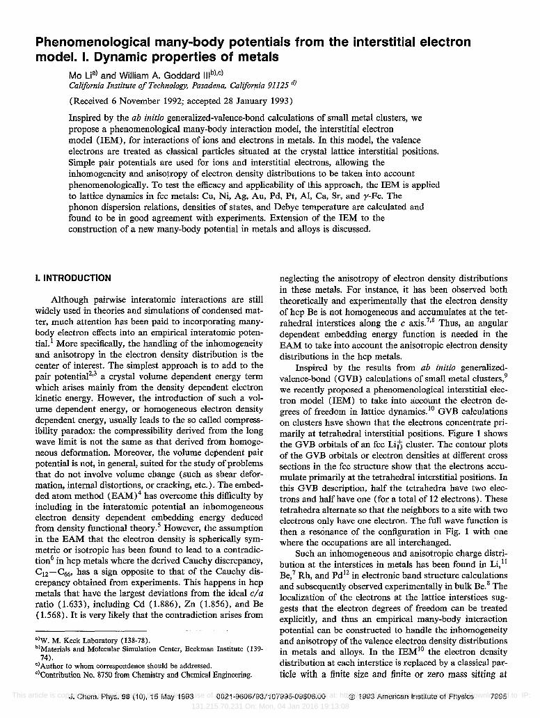
FIG. 2. Phonon dispersion curves for Cu. Dots represent experimental data. Solid lines are for the fluorite structure.
Service of AlP .27 Interested readers can obtain these results from there.
v. LATTICE DYNAMICS
In the traditional Born-von Karman method, the second derivatives of the potential energy with respect to the atom displacements are used as empirical parameters in the study of lattice dynamics. A satisfactory fit of experimental phonon dispersions by this method usually needs many such parameters, making the interaction range of the interatomic potentials extremely long. It is not desirable to have long range interatomic interactions. The physical meaning of an interatomic potential having five to ten nearest neighbors becomes questionable. Microscopic theories, on the other hand, are able to provide detailed understanding of lattice vibrations by explicitly including the electrons, but their complicated formalisms usually make it very difficult to calculate the phonon dispersions and thermophysical properties. For instance, the recently developed frozen-phonon method28 could handle transition metals, but complications in computing the total energies make the calculated phonon dispersions available only at the wave vectors commensurate with the ion displacements. It would, therefore, be desirable to have lattice dynamics models which, on one hand, have a simple formalism for the numerical calculations and, on the other hand, still retain the important many-body effects. There are a growing number of such lattice dynamics models, for example, the shell model29 for ionic solids and the adiabatic bond charge model3o for covalent bond solids, the thirdorder perturbation method31 for transition metals, and so on. The IEM bears the same key feature as these models: the valence electrons are treated as fictitious classical particles and the interatomic or interion interactions are modulated by the presence of these electrons. The vibration spectra, densities of states, and Debye temperature are calculated using IEM and presented as follows.
r !J. X 1: r-A-L 10.0
AI [100] ,- [111] f "'" [110] /1 I
>!~! V
N 8.0
jl l .r=
i t:.. ~I ",\ 6.0 8 j/ i~ I >- !
I 1---1 0 Y" ""I C 4.0 Q) ::J
~. 0- !/" t .X Q) I-
/ LL
"
0.2 0.4 0.6 0.8 1.0 0.8 0.6 0.4 0.0 0.2 0.4
q/q[100]- -- q/q[110] q/q[111l
Reduced Wave Vector
FIG. 3. Phonon dispersion curves for AI.
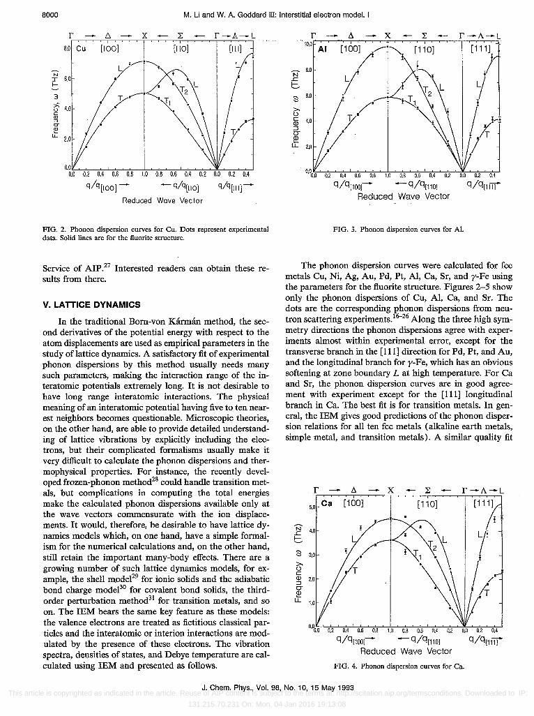
The phonon dispersion curves were calculated for fcc metals Cu, Ni, Ag, Au, Pd, Pt, AI, Ca, Sr, and y-Fe using the parameters for the fluorite structure. Figures 2-5 show only the phonon dispersions of Cu, AI, Ca, and Sr. The dots are the corresponding phonon dispersions from neutron scattering experiments. I6-26 Along the three high symmetry directions the phonon dispersions agree with experiments almost within experimental error, except for the transverse branch in the [111] direction for Pd, Pt, and Au, and the longitudinal branch for y-Fe, which has an obvious softening at zone boundary L at high temperature. For Ca and Sr, the phonon dispersion curves are in good agreement with experiment except for the [111] longitudinal branch in Ca. The best fit is for transition metals. In general, the IEM gives good predictions of the phonon dispersion relations for all ten fcc metals (alkaline earth metals, simple metal, and transition metals). A similar quality fit
N .r= t:.. 8 >-0 c Q) ::J 0-~
LL
r !J. - X 1:
5.0 Ca [100] [110]
4.0
3.0
2.0
0.2 0.4 0.6 0.8 1.0 0.8 0.6 0.4
Q/q[100]--- Q/Q[110]
Reduced Wave Vector
0.0 0.2 0.4
Q/Q[111l
FIG. 4. Phonon dispersion curves for Ca.
J. Chern. Phys., Vol. 98, No. 10, 15 May 1993 This article is copyrighted as indicated in the article. Reuse of AIP content is subject to the terms at: http://scitation.aip.org/termsconditions. Downloaded to IP:
131.215.70.231 On: Mon, 04 Jan 2016 19:13:08
M. Li and W. A. Goddard III: Interstitial electron model. I 8001
[" /). - X ~ [" -A-L 4.0 ""~~'-"~"-"--'-':'-~~""""''''''~-r-T--,.-''''-r-r-r-i
Sr [100] [110] [111]
N 3.0 .c t:.. 8 >- 2.0 () C Q) ::J cr Q) 1.0 ....
LL
0.2 0.4 0.6 O.S 1.0 O.S 0.6 0.4 0.0 0.2 0.4
q/q[100]- -- Q/Q[110l q/q[111]
Reduced Wave Vector
FIG. 5. Phonon dispersion curves for Sr.
using the traditional force constant model in the atomcentered scheme, would need at least eight sets of nearest neighbors.32
The off-symmetry phonon dispersions of Cu are calculated and can be obtained from the Physics Auxiliary Publication Service. It was found33 that using atom-centered pair potential models with force constants obtained by fitting experimental phonon dispersion curves along the high symmetry directions, the lattice dynamics do not necessarily predict the vibration frequencies in off-symmetry directions. Using the IEM, we find that the calculated phonon frequencies in the off-symmetry directions agree with the measured ones very well.
To calculate other thermophysical properties, one needs to know the phonon densities of states. The densities of states were computed for all fcc metals and displayed in Figs. 6-9 for Cu, AI, Ca, and Sr. Figure 10 shows the calculated Debye temperature for Cu, using the calculated density of states in Fig. 6. One can see that it agrees quite well with the experiments.33,34
Despite these good results with !EM, it remains to be shown that the !EM is capable of treating the many-body effects (phonon dispersions in fcc metals are quite simple). A more stringent test was conducted recently by Schultz and MessmerY Using the IEM, they successfully fit the phonon dispersions in the intermetallic compound Ni3Al with as few as 12 parameters. Their results demonstrate that the IEM is able to predict dynamic properties of complicated systems, Further tests still need to be done to check effects on dynamic properties of not only different structures such as bcc and hcp, but also long range interactions ignored in the present simple model.
VI. CONCLUSIONS
We have proposed and tested the interstitial electron model for lattice dynamics .in metals. This model is inspired by results from calculations of small metal clusters using the ab initio generalized-valence-bond method. We calculated the phonon dispersions, densities of states, and Debye temperature for most fcc metals in the periodic table. The results are quite encouraging. However, since the specific form of the IEM used here is oversimplified (only
2 1.0 .s U)
a .2:- 0.5 'en c:: Q)
Cl 0.00.0 .
Ca: Nk = 1,873,761
Nro = 1,031
1.0 2.0 3.0 4.0 w (THz)
FIG. 8. Phonon density of states for Ca.
6.0' .
J. Chern. Phys., Vol. 98, No. 10, 15 May 1993 This article is copyrighted as indicated in the article. Reuse of AIP content is subject to the terms at: http://scitation.aip.org/termsconditions. Downloaded to IP:
131.215.70.231 On: Mon, 04 Jan 2016 19:13:08
8002 M. Li and W. A. Goddard III: Interstitial electron model. I
22 § 2.5
2:-~
Sr: Nk = 1,873,761
Nw= 641
~--tron distribution to the interatomic interaction, as demonstrated by the IEM, will motivate further investigations along this direction.
nearest-neighbor terms), these results merely demonstrate the applicability of IBM. Extending this model to use long range interactions is straightforward.
Because the key assumption that the electrons are localized at the lattice interstitial sites is based on results from small cluster calculations, it remains uncertain whether the IEM is able to predict bulk properties and whether it can be generalized to other metals and alloys. To judge its validity and universality would require ab initio calculations using correlated wave functions on very large, bulklike systems. Nevertheless, other theoretical or experimental approaches have provided some interesting results that support the assumption of localization of valence electrons in lattice interstices. For instance, band structure caIcuiations7,9,12 and x-ray measurements8 indicate that the electron accumulation at the tetrahedral interstices is not an artifact arising from the small cluster size effect or reSUlting from a particular technique used, but a natural consequence of electron many-body interactions. Unfortunately, real space distributions of the electron density are often not available from experiment. We hope that the importance of the anisotropic and inhomogeneous elec-
FIG. 10. Calculated Debye temperature for Cu. Experimental data are from Ref. 32 (dots) and 33 (triangles).
In order to determine whether the IEM can predict other bulk properties, further tests are necessary. Like any other empirical interatomic interaction, the IEM is a phenomenological model. Its merits are based on simplicity and the ability to predict a variety of physical properties. It will be useful to apply it to realistic problems such as the above- mentioned Cauchy discrepancy in hcp metals, surface structures, transport properties, structures of defects, and so on. This work is in progress.
ACKNOWLEDGMENTS
This work was initiated with support from a grant from the National Science Foundation-Materials Research Groups (Grant No. DMR-8811795) and finished with support from NSF-CHE-91-100284. The facilities of the MSC/BI are supported also by grants from DOE-AI CD, Allied Signal, ASAHI Chemical, ASAHI Glass, BP America, Chevron, Xerox Corp., and Beckman Institute.
I Many-Atom Interactions in Solids, edited by R. M. Nieminen, M. J. Puska, and M. J. Manninen (Springer-Verlag, Berlin, 1990); Atomistic Simulation of Materials beyond Pair Potentials, edited by V. Vitek and D. J. Srolovitz (Plenum, New York, 1989); Interatomic Potentials and Crystalline Defects, edited by J. K. Lee (AIME, Warrendale, PA, 1981).
2K. Fuchs, Proc. R. Soc., London Ser. B 153, 622 (1936); R. A. Johnson, Phys. Rev. B 6, 2094 (1972).
3 W. A. Harrison, Electronic Structure and the Properties of Solids (Free-man, San Francisco, 1980).
4M. S. Daw and M. I. Baskes, Phys. Rev. B 29,6443 (1984). sp. Hohenberg and w. Kohn, Phys. Rev. B 136, 864 (1964). 6M. Li and W. A. Goddard III (unpublished results). 7S. T. Inoue and J. Y. Yamashita, J. Phys. Soc. Jpn. 35, 677 (1973); R.
Dovesi et al., Phys. Rev. B 25, 3731 (1982) and M. Y. Chou, P. K. Lam, and M. L. Cohen, ibid. 28, 4179 (1983).
SF. K. Larsen and N. K. Hansen, Acta Crystallogr. B 40, 169 (1984); L. Massa et aI., Phys. Rev. Lett. 55, 622 (1985).
9 (a) M. H. McAdon and W. A. Goddard, Phys. Rev. Lett. 55, 2563 (1985); (b) J. Phys. Chern. 91, 2607 (1987).
10M. Li and W. A. Goddard, Phys. Rev. B 40, 12155 (1989). IIR. Dovesi et aI., Z. Phys. B 51, 195 (1983). 12p. A. Schultz and R. P. Messmer, Phys. Rev. B 45, 7467 (1992). 13 P. Bruesch, Phonons: Theory and Experiments, Springer Series in Solid
State Science 34 (Springer-Verlag, Berlin, Heidelberg, 1982); A. A. Maradudin, E. W. Montroll, G. H. Weiss, and I. P. Ipatova, Theory of Lattice Dynamics in the Harmonic Approximation, 2nd ed. (Academic, New York, 1971).
14M. Born and K. Huang, Dynamical Theory of Crystal Lattice (Oxford University, London, New York, 1954), p. 136.
15W. B. Pearson, Handbook of Lattice Spacings and Structures of Metals and Alloys (Pergamon, Oxford, 1967); R. O. Simmons and H. Wang, Single Crystal Elastic Constants and Calculated Aggregate Properties: A Handbook (MIT, Cambridge, 1971).
16U. Buchenau,M. Heiroth, H. R. Schober et aL, Phys. Rev. B 30, 3502 (1984).
17R. Stedman, L. Almqvist, and G. Nilsson, Phys. Rev. 162, 549 (1967). ISR. J. Birgeneau, J. Cordes, G. Dolling, and A. D. B. Woods, Phys. Rev.
A 13, 1359 (1964). 19E. C. Svensson, B. Brockhouse, and J. M. Rowe, Phys. Rev. 155, 619
(1967). 20 A. P. Miller and B. N. Brockhouse, Can. J. Phys. 4, 704 (1971). 21 W. A~ Kamitakahara and B. N. Brockhouse, Phys. Lett. 2A, 639
(1969). 22R. Ohrlich and W. Drexel, 4th IAEA Symp. Inelastic Scattering of
Neutrons, Vol. 1 (IAEA, Vienna, 1968), p. 203.
J. Chern. Phys., Vol. 98, No. 10, 15 May 1993 This article is copyrighted as indicated in the article. Reuse of AIP content is subject to the terms at: http://scitation.aip.org/termsconditions. Downloaded to IP:
131.215.70.231 On: Mon, 04 Jan 2016 19:13:08
M. Li and W. A. Goddard III: Interstitial electron model. I 8003
23 J. W. Lynn, H. G. Smith, and R. M. Nicklow, Phys. Rev. B 8, 3493 (1973).
24J. Zarestky and C. Stassis, Phys. Rev. B 35, 4500 (1987). 2sR. Stedman and G. Nilsson, Phys. Rev. 145, 492 (1966). 26C. Stassis, J. Zaretsky, D. K. Misemer, H. L. Skriver, and B. N. Har
mon, Phys. Rev. B 27,3303 (1983). 27See AlP document no. PAPS JCPSA-98-7995-19 for 19 pages of tables
and figures. Order by PAPS number and journal reference from American Institute of Physics, Physics Auxiliary Publication Service, 335 East 45th Street, New York, NY 10017. The price is $1.50 for each microfiche (60 pages) or $5.00 for photocopies of up to 30 pages, and
$0.15 for each additional page over 30 pages. Airmail additional. Make checks payable to the American Institute of Physics.
28K._M. Ho, C. L. Fu, and B. N. Harmon, Phys. Rev. B 2,1575 (1984). 29W. Cochran, Phys. Rev. Lett. 2, 495 (1959). 30W. Weber, Phys. Rev. Lett. 33, 371 (1974). 31 D. Prakash and J. C. Upadhyaya, J. Phys. Chem. Solids 49,91 (1988). 32G. Gilat and R. M. Nicklow, Phys. Rev. 143,487, (1966). 33D. L. Martin, Can. J. Phys. 38, 17 (1960). 34T. C. Cetas, C. R. Tilford, and C. A. Swenson, Phys. Rev. 174,
835 (1968).
J. Chern. Phys., Vol. 98, No. 10, 15 May 1993 This article is copyrighted as indicated in the article. Reuse of AIP content is subject to the terms at: http://scitation.aip.org/termsconditions. Downloaded to IP: