Phenomenology of loop quantum cosmology

This content has been downloaded from IOPscience. Please scroll down to see the full text.

Download details:

IP Address: 132.203.227.63

This content was downloaded on 28/06/2014 at 13:02

Please note that terms and conditions apply.

Phenomenology of loop quantum cosmology

View the table of contents for this issue, or go to the journal homepage for more

2010 J. Phys.: Conf. Ser. 222 012027

(http://iopscience.iop.org/1742-6596/222/1/012027)

Home Search Collections Journals About Contact us My IOPscience

iopscience.iop.org/page/terms

http://iopscience.iop.org/1742-6596/222/1

http://iopscience.iop.org/1742-6596

http://iopscience.iop.org/

http://iopscience.iop.org/search

http://iopscience.iop.org/collections

http://iopscience.iop.org/journals

http://iopscience.iop.org/page/aboutioppublishing

http://iopscience.iop.org/contact

http://iopscience.iop.org/myiopscience

Phenomenology of loop quantum cosmology

Mairi SakellariadouDepartment of Physics, King’s College London, University of London, Strand WC2R 2LS, UK

E-mail: [email protected]

Abstract. After introducing the basic ingredients of Loop Quantum Cosmology, I will brieflydiscuss some of its phenomenological aspects. Those can give some useful insight about the fullLoop Quantum Gravity theory and provide an answer to some long-standing questions in earlyuniverse cosmology.

1. IntroductionThe variety of precise astrophysical and cosmological data, available at present, combined withthe large number of high energy physics experiments, are expected to give us the necessaryingredients to test fundamental theories and understand the very early phases of the evolutionof our universe.

Cosmological inflation [1] remains the most promising candidate to solve the shortcomingsof the standard hot big bang model, while it offers a causal explanation for the primordialfluctuations with the correct Cosmic Microwave Background (CMB) features. Despite thissuccess, inflation suffers from a number of drawbacks [2]. In particular, compatibility betweentheory and measurements often necessitates fine-tuning of the inflationary parameters, inflationremains still a paradigm in search of a model, while it must prove itself generic [3, 4, 5, 6, 7, 8, 9].

There is undoubtfully an additional list of fundamental cosmological questions, still lackinga satisfying answer. One does not know, for instance, how close to the big bang a smoothspace-time can be considered as the correct framework. Quantum gravity, a full theory which issupposed to resolve the big bang singularity, is still missing, while it is not known whether a newboundary condition is needed at the big bang, or whether quantum dynamical equations remainwell-behaved at singularities. It is nevertheless clear that a smooth space-time backgroundcannot be assumed as the correct description close to the big bang.

In a Hamiltonian formulation to a quantum theory, the absence of background metricindicates that Hamiltonian dynamics is generated by constraints. Physical states are solutionsto quantum constraints implying that all physical laws are obtained from these solutions, whilethere is no external time according which evolution can be studied. One has to define a monotonicvariable to play the role of emergent, or internal, time, and then build a framework within whichthe short-distance drawbacks of General Relativity near the big bang can be cured, maintaininghowever the agreement with General Relativity at large scales.

Loop Quantum Gravity (LQG) [10, 11] is a non-perturbative and background independentcanonical quantisation of General Relativity in four space-time dimensions. Loop QuantumCosmology (LQC) [12] is a cosmological mini-superspace model quantised with methods ofLQG. The discreteness of spatial geometry and the simplicity of the setting allow for a complete

First Mediterranean Conference on Classical and Quantum Gravity (MCCQG 2009) IOP PublishingJournal of Physics: Conference Series 222 (2010) 012027 doi:10.1088/1742-6596/222/1/012027

c© 2010 IOP Publishing Ltd 1

study of dynamics. The difference between LQC and other approaches of quantum cosmology,is that the input is motivated by a full quantum gravity theory. The simplicity of the setting,combined with the discreteness of spatial geometry provided by LQG, render feasible the overallstudy of LQC dynamics.

In what follows, I will briefly discuss some of the phenomenological consequences of LQC,a subject which gains constantly an increasing interest from the scientific community, due inparticular to its successes.

2. Elements of LQG/LQCLoop quantum cosmology is formulated in terms of SU(2) holonomies of the connection andtriads. The canonically conjugated variables are defined by the densitised triad Ea

i , and anSU(2) valued connection Ai

a, where i refers to the Lie algebra index, and a is a spatial indexwith a, i = 1, 2, 3. The densitised triad gives information about spatial geometry (i.e., the threemetric), while the connection gives information about curvature (spatial and extrinsic one).Let me explain this: Quantum gravity introduces a discreteness to space-time. To quantisequantum gravity, this discreteness manifests itself as quanta of space. Since the quanta are three-dimensional, they can be characterised by a triad of numbers. The connection between adjacentpairs of these quanta form a two-dimensional surface, through which the geometric connection isdefined. To ensure that local rotations do not induce different geometries, this connection mustbe SO(3) invariant. By using connection-triad variables, arising from a canonical transformationof Arnowitt-Desner-Misner ( variables, one can make an analogy with gauge theories, which isparticularly useful when dealing with quantisation issues.

For any quantisation scheme based on a Hamiltonian framework (e.g., LQC) or an actionprinciple (e.g., path integral) for a homogeneous and flat model, divergences appear which needto be regularised. To remove the divergences that occur in non-compact topologies, the spatialhomogeneity and Hamiltonian are restricted to a finite fiducial cell, of scale µ0, with finite volumeV0 =

∫d3x

√|0q|, where 0q is the determinant of the fiducial background metric.

In the case of a spatially flat background, derived from the Bianchi I model, the isotropicconnection can be expressed in terms of the dynamical component of the connection c(t) as

Aia = c(t)ωi

a , (1)

with ωia a basis of left-invariant one-forms ωi

a = dxi. The densitised triad can be decomposedusing the Bianchi I basis vector fields Xa

i = δai as

Eai =

√0qp(t)Xa

i , (2)

where 0q stands for the determinant of the fiducial background metric 0qab = ωiaωbi, and p(t)

denotes the remaining dynamical quantity after symmetry reduction.In terms of the metric variables with three-metric qab = a2ωi

aωbi, the dynamical quantity isjust the scale factor a(t). Given that the Bianchi I basis vectors are Xa

i = δai ,

|p| = a2 , (3)

where the absolute value is taken because the triad has an orientation. Since the basis vectorfields are spatially constant in the spatially flat model, the connection component is

c = sgn(p)γa

N; (4)

N is the lapse function and γ the Barbero-Immirzi parameter, a quantum ambiguity parameterapproximately equal to 0.2375.


2

The canonical variables c, p are related through the Poisson bracket

{c, p} =κγ

3V0 , (5)

where V0 the volume of the elementary cell adapted to the fiducial triad and κ ≡ 8πG.Defining the triad component p, determining the physical volume of the fiducial cell, and

the connection component c, determining the rate of change of the physical edge length of thefiducial cell, as

p = V2/30 p , c = V

1/30 c , (6)

respectively, we obtain{c, p} =

κγ

3, (7)

independent of the volume V0 of the fiducial cell.To quantise the theory one faces the usual difficulty of quantum cosmology. Namely, the

metric itself has to be considered as a physical field, thus it must be quantised; it is not afixed background. Any standard quantisation scheme fails: Fock quantisation fails, while evenfree Hamiltonians are non-quadratic in metric dependence, so there is no simple perturbationanalysis. The way out is to use gauge theory variables to define holonomies of the connectionalong a given edge

he(A) = P exp∫

dsγµ(s)Aiµ(γ(s))τi , (8)

where P indicates a path ordering of the exponential, γµ is a vector tangent to the edge andτi = −iσi/2, with σi the Pauli spin matrices, and fluxes of a triad along an S surface

E(S, f) =∫

SεabcE

cifidxadxb , (9)

with fi an SU(2) valued test function. Certainly, at the level of LQC these variables may seemad-hoc and unnatural, however their motivation follows naturally from the full LQG theory.

Thus, the basic configuration variables in LQC are holonomies of the connection

h(µ0)i (A) = cos

(µ0c

2

)1 + 2 sin

(µ0c

2

)τi , (10)

along a line segment µ00ea

i and the flux of the triad

FS(E, f) ∝ p ,

where the basic momentum variable is the triad component p, 1 is the identity 2× 2 matrix andτi = −iσi/2 is a basis in the Lie algebra SU(2) satisfying the relation

τiτj = (1/2)εijkτk − (1/4)δij .

In the classical theory, curvature can be expressed as a limit of the holonomies around a loopas the area enclosed by the loop shrinks to zero. In quantum geometry however, the loop cannotbe continuously shrunk to zero area and the eigenvalues of the area operator are discrete. Thus,there is a smallest non-zero eigenvalue, the area gap ∆ [13]. As a result, the Wheeler-de Wittdifferential equation gets replaced by a difference equation whose step size is controlled by ∆.

Let me start with the old quantisation procedure. Along the lines of LQG, one considerseiµ0c/2 (with µ0 an arbitrary real number) and p, as the elementary classical variables, which


3

have well-defined analogues. Using the Dirac bra-ket notation and setting eiµ0c/2 = 〈c|µ〉, theaction of the operator p acting on the basis states |µ〉 reads

p|µ〉 =κγ~|µ|

6|µ〉 , (11)

where µ (a real number) stands for the eigenstates of p, satisfying the orthonormality relation

〈µ1|µ2〉 = δµ1,µ2 . The action of the

exp[

iµ0

2 c]

operator acting on basis states |µ〉 is

exp

[iµ0

2c

]|µ〉 = exp

[µ0

ddµ

]|µ〉 = |µ + µ0〉 , (12)

where µ0 is any real number. Thus, in the old quantisation, the operator eiµ0c/2 acts as a simpleshift operator. As in the full LQG theory, there is no operator corresponding to the connection,however the action of its holonomy is well defined. The action of the holonomies, h

(µ0)i , of the

gravitational connection on the basis states is given by [14]

h(µ0)i |µ〉 = (cs1 + 2snτi) |µ〉 , (13)

where,

cs|µ〉 ≡ cos(µ0c/2)|µ〉 = [ |µ + µ0〉+ |µ− µ0〉 ] /2 ,

sn|µ〉 ≡ sin(µ0c/2)|µ〉 = [ |µ + µ0〉 − |µ− µ0〉 ] /(2i) . (14)

The gravitational part of the Hamiltonian operator in terms of SU(2) holonomies and thetriad component, in the irreducible J = 1/2 representation, reads [14]

Cg =2i

κ2~γ3µ30

tr∑

ijk

εijk(h

(µ0)i h

(µ0)j hi(µ0)−1h

(µ0)−1j h

(µ0)k

[h

(µ0)−1k , V

])sgn(p) . (15)

The action of the self-adjoint Hamiltonian constraint operator, Hg = (Cg + C†g)/2 on the basisstates |µ〉 is

Hg|µ〉 =3

4κ2γ3~µ30

{[R(µ)+R(µ+4µ0)

]|µ+4µ0〉−4R(µ)|µ〉+ [R(µ)+R(µ−4µ0)

]|µ−4µ0〉}

,

(16)where

R(µ) = (κγ~/6)3/2∣∣∣|µ + µ0|3/2 − |µ− µ0|3/2

∣∣∣ . (17)

The dynamics are then determined by the Hamiltonian constraint

(Hg + Hφ)|Ψ〉 = 0 , (18)

where Hφ stands for the matter Hamiltonian. In the full LQG theory there is an infinite numberof constraints, while in LQC there is only one integrated Hamiltonian constraint. Matter isintroduced by just adding the actions of matter components to the gravitational action. We canfinally obtain difference equations analogous to the differential Wheeler-de Witt equations.


4

More precisely, the constraint equation on the physical wave-functions |Ψ〉, which can beexpanded using the basis states as |Ψ〉 =

∑µ Ψµ(φ)|µ〉 with summation over values of µ and

where the dependence of the coefficients on φ represents the matter degrees of freedom, reads [15][∣∣∣Vµ+5µ0 − Vµ+3µ0

∣∣∣ +∣∣∣Vµ+µ0 − Vµ−µ0

∣∣∣]Ψµ+4µ0(φ)− 4

∣∣∣Vµ+µ0Vµ−µ0

∣∣∣Ψµ(φ)

+

[∣∣∣Vµ−3µ0 − Vµ−5µ0

∣∣∣ +∣∣∣Vµ+µ0 − Vµ−µ0

∣∣∣]Ψµ−4µ0(φ) = −4κ2γ3~µ3

0

3Hφ(µ)Ψµ(φ) ; (19)

the matter Hamiltonian Hφ is assumed to act diagonally on the basis states with eigenvaluesHφ(µ). Equation (19) is the quantum evolution (in internal time µ) equation; there is nocontinuous variable (the scale factor in classical cosmology), but a label µ with discrete steps.The wave-function Ψµ(φ), depending on internal time µ and matter fields φ, determines thedependence of matter fields on the evolution of the universe, with a massless scalar field playingthe role of emergent time. Thus, in LQC the quantum evolution is governed by a second orderdifference equation, rather than the second order differential equation of the Wheeler-de Wittquantum cosmology. As the universe becomes large and enters the semi-classical regime, itsevolution can be approximated by the differential Wheeler-de Witt equation.

3. Lattice refinementThe quantised holonomies were at first assumed to be shift operators with a fixed magnitude,leading to a quantised Hamiltonian constraint being a difference equation with a constant intervalbetween points on the lattice. While these models can be used to study certain aspects of thequantum regime, they were found to lead to serious instabilities in the continuum, semi-classicallimit [16, 17]. Considering the continuum limit of the Hamiltonian constraint operator, wehave so far assumed that Ψ does not vary much on scales of the order of 4µ0 (known as pre-classicality), so that one can smoothly interpolate between the points on the discrete functionΨµ(φ) and approximate them by the continuous function Ψ(µ, φ). Under this assumption, thedifference equation can be very well approximated by a differential equation for a continuouswave-function. However, the form of the wave-function indicates that the period of oscillationscan decrease as the scale increases. Thus, the assumption of pre-classicality can break down atlarge scales, leading to deviations from the classical behaviour.

Let me explain this point a bit further: In the underlying full LQG theory, the contributionsto the (discrete) Hamiltonian operator depend on the state which describes the universe. Asthe volume grows (ı.e., the universe expands), the number of contributions increases. Thus, theHamiltonian constraint operator is expected to create new vertices of a lattice state (in additionto changing their edge labels), which in LQC results in a refinement of the discrete lattice [18].Lattice refinement is also required from phenomenological reasons [17, 19]; for instance, it rendersa successful inflationary era more natural [19]. The effect of lattice refinement has been modelledand the elimination of the instabilities in the continuum era has been explicitly shown.

The appropriate lattice refinement model should be obtained from the full LQG theory. Inprinciple, one should use the full Hamiltonian constraint and find the way that its action balancesthe creation of new vertices as the volume increases. Instead, phenomenological arguments havebeen used, where the choice of the lattice refinement model is constrained by the form of thematter Hamiltonian [20]. In particular, LQC can generically support inflation, and other matterfields, without the onset of large scale quantum gravity corrections, only for a particular model oflattice refinement [20]. This choice is the only one for which physical quantities are independentof the elementary cell adopted to regulate spatial integrations [21], and moreover, it is exactly thechoice required for the uniqueness of the factor ordering of the Wheeler-de Witt equation [22].


5

Allowing the length scale of the holonomies to vary dynamically, the form of the differenceequation, describing the evolution, changes. Since the parameter µ0 determines the step-sizeof the difference equation, assuming the lattice size is growing, the step-size of the differenceequation is not constant in the original triad variables. Let us consider the particular case of

µ0 → µ (µ) = µ0µ−1/2 , (20)

suggested by certain intuitive heuristic approaches, such as noting that the minimum area usedto regulate the holonomies should be a physical area [23], or that the discrete step size ofthe difference equation should always be of the order of the Planck volume. Moreover, thischoice also results in a significant simplification of the difference equation, compared to moregeneral lattice refinement schemes. The basic operators are given by replacing µ0 with µ. Uponquantisation [23]

eiµc/2|µ〉 = e−iµ d

dµ |µ〉 , (21)

which is no longer a simple shift operator since µ is a function of µ. Changing the basis to

ν = µ0

∫dµ

µ=

23µ3/2 , (22)

one getse−iµ d

dµ |ν〉 = e−iµ0ddν |ν〉 = |ν + µ0〉 . (23)

Thus, in the new variables the holonomies act as simple shift operators, with parameter lengthµ0. In this sense, the basis |ν〉 is a much more natural choice than |µ〉. One can then proceedas in the previous case of a fixed spatial lattice and write down the Hamiltonian constraint.

3.1. Constraints on inflationLet me consider first a fixed and then a dynamically varying lattice and solve the second orderdifference equation in the continuum limit. Two constraints can be imposed on the inflatonpotential: the first one so that the continuum approximation is valid, and the second one sothat there is agreement with the CMB measurements on large angular scales. A combinationof the two constraints in the context of a particular inflationary model, will give us [20] theconditions for natural and successful inflation within LQC.

More precisely, let us separate the wave-function Ψ(p, φ) into Ψ(p, φ) = Υ(p)Φ(φ) andapproximate the dynamics of the inflaton field, φ, by setting V (φ) = Vφpδ−3/2, where Vφ isa constant and δ = 3/2 in the case of slow-roll, to get [20]

p−1/2 ddp

[p−1/2 d

dp

(p3/2Υ (p)

)]+ βVφpδΥ(p) = 0 , (24)

with solutions [20]

Υ (p) ≈ p−(9+2δ)/8

√2δ + 3

2√

βVφπ

[C1 cos

(x− 3π

2(2δ + 3)− π

4

)+ C2 sin

(x− 3π

2(2δ + 3)− π

4

)],

(25)where x = 4

√βVφ(2δ + 3)−1p(2δ+3)/4 and β = 96/(κ~2).

Without lattice refinement, the discrete nature of the underlying lattice would eventuallybe unable to support the oscillations and the assumption of pre-classicality will break down,implying that the discrete nature of space-time becomes significant on large scales. For the endof inflation to be describable using classical General Relativity, it must end before a scale, at


6

which the assumption of pre-classicality breaks down and the semi-classical description is nolonger valid, is reached. Let me quantify this constraint: The separation between two successivezeros of Υ (p) is

∆p =π√βVφ

p(1−2δ)/4 . (26)

For the continuum limit to be valid, the wave-function must vary slowly on scales of the orderof µc = 4µ, leading to [20]

∆p > 4µ0

(κγ~6

)3/2

p−1/2 , (27)

which implies [20]

Vφ <27π2

192µ20γ

3κ2~p(3−2δ)/2 . (28)

Assuming slow-roll inflation, we set δ ≈ 3/2. Setting µ0 = 3√

3/2, the constraint on theinflationary potential, in units of ~ = 1, reads

V (φ) <∼ 2.35× 10−2l−4Pl , (29)

which is a weaker constraint than the one imposed for fixed lattices, namely [20]

Vφ ¿ 10−28l−4pl , (30)

assuming that half of the inflationary era takes place during the classical era.One can further constrain the inflationary potential so that the fractional over-density in

Fourier space and at horizon crossing is consistent with the COBE-DMR measurements, namely

[V (φ)]3/2

V ′(φ)≈ 5.2× 10−4M3

Pl . (31)

To do so, one must however adopt a particular inflationary model. As such, let us selectV (φ) = m2φ2/2. Combining the two constraints we obtain [20]

m <∼ 70(e−2Ncl) MPl and m <∼ 10 MPl , (32)

for the fixed and varying lattices, respectively.In conclusion, the requirement that a significant proportion of a successful (in particular

with respect to the CMB measurements) inflationary regime takes place during the classical era,imposes a strong constraint on the inflaton mass. Such a constraint turns out however to bemuch softer, and therefore rather natural, once lattice refinement is considered. In this sense,we argue [20] that lattice refinement is essential to achieve a successful inflationary era, providedinflation can be generically (i.e., with generic initial conditions) realised.

3.2. Constraints on the matter HamiltonianGiven a lattice refinement model, we will show [19] that only certain types of matter can beallowed. To do so, we parametrise the lattice refinement by A and the matter Hamiltonianby δ and solve the Hamiltonian constraint. The restrictions on the two-dimensional parameterspace will become apparent once physical restrictions to the solutions of the wave-functions areimposed [19].

To be more precise, considerµ = µ0µ

A , (33)


7

-0.5

-0.4

-0.3

-0.2

-0.1

0

-1.5 -1 -0.5 0 0.5 1 1.5 2

A

δ

Break down ofpreclassicality

Non-normalisable

Limit ofBessel Expansion

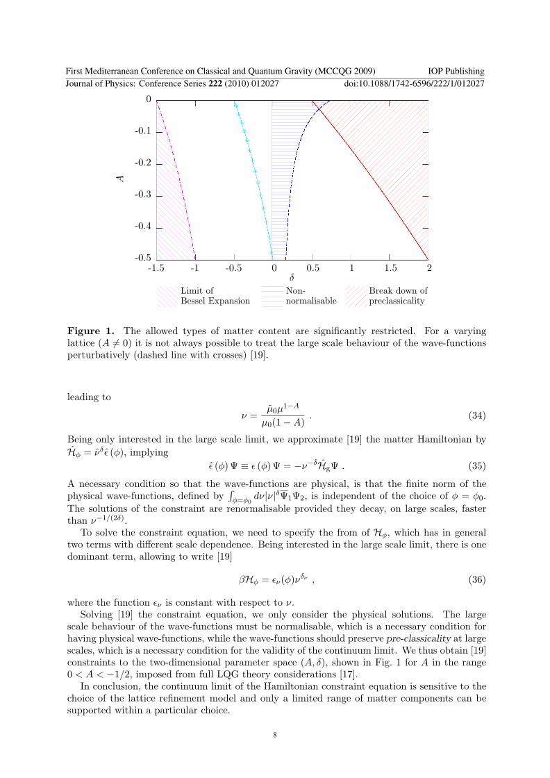
Figure 1. The allowed types of matter content are significantly restricted. For a varyinglattice (A 6= 0) it is not always possible to treat the large scale behaviour of the wave-functionsperturbatively (dashed line with crosses) [19].

leading to

ν =µ0µ

1−A

µ0(1−A). (34)

Being only interested in the large scale limit, we approximate [19] the matter Hamiltonian byHφ = νδ ε (φ), implying

ε (φ)Ψ ≡ ε (φ)Ψ = −ν−δHgΨ . (35)

A necessary condition so that the wave-functions are physical, is that the finite norm of thephysical wave-functions, defined by

∫φ=φ0

dν|ν|δΨ1Ψ2, is independent of the choice of φ = φ0.The solutions of the constraint are renormalisable provided they decay, on large scales, fasterthan ν−1/(2δ).

To solve the constraint equation, we need to specify the from of Hφ, which has in generaltwo terms with different scale dependence. Being interested in the large scale limit, there is onedominant term, allowing to write [19]

βHφ = εν(φ)νδν , (36)

where the function εν is constant with respect to ν.Solving [19] the constraint equation, we only consider the physical solutions. The large

scale behaviour of the wave-functions must be normalisable, which is a necessary condition forhaving physical wave-functions, while the wave-functions should preserve pre-classicality at largescales, which is a necessary condition for the validity of the continuum limit. We thus obtain [19]constraints to the two-dimensional parameter space (A, δ), shown in Fig. 1 for A in the range0 < A < −1/2, imposed from full LQG theory considerations [17].

In conclusion, the continuum limit of the Hamiltonian constraint equation is sensitive to thechoice of the lattice refinement model and only a limited range of matter components can besupported within a particular choice.


8

3.3. Uniqueness of the factor ordering in the Wheeler-de Witt equationI will now show that the lattice refinement model µ = µ0µ

−1/2, argued [22] to be the onlyone achieved by both physical considerations of large scale physics and consistency of thequantisation structure, is also the only model which makes the factor ordering ambiguities ofLQC to disappear in the continuum limit [22].

Let me be more specific. Writing the gravitational part of the Hamiltonian constraint interms of the triad and the holonomies of the connection, one realises that there are many waysof doing so. Considering for example,

Cg =2i

κ2~γ3k3tr

∑

ijk

εijk(hihjh

−1i h−1

j hk

[h−1

k , V])

, (37)

there are many possible choices of factor ordering that could have been made at this point;classically, the actions of the holonomies commute. However, each of these factor orderingchoices leads to a different factor ordering of the Wheeler-de Witt equation in the continuumlimit. The action of the factor ordering chosen in Eq. (37) leads [22] to

εijktr(hihjh

−1i h−1

j hk

[h−1

k , V])

= −24sn2cs2(csV sn− snV cs

), (38)

while other choices have certainly a different action.Defining V |ν〉 = Vν |ν〉, with V the volume operator with eigenvalues Vν , the action of the

above factor ordering on a general state |Ψ〉 =∑

ν ψν |ν〉 in the Hilbert space, reads [22]

εijktr(hihjh

−1i h−1

j hk

[h−1

k , V])|Ψ〉 =

−3i

4

∑ν

[(Vν−3k − Vν−5k

)ψν−4k − 2

(Vν+k − Vν−k

)ψν

+(Vν+5k − Vν+3k

)ψν+4k

]|ν〉 ; (39)

the action of any other factor ordering choice can be obtained in a similar manner. By notingthat the volume is given by

Vν |ν〉 ∼ [µ (ν)]3/2|ν〉 , (40)

where µ(ν) is obtained by

ν =kµ1−A

µ0(1−A), (41)

we find [22]

Vν±nk ∼[(ν ± nk)α

]3/[2(1−A)], (42)

where α = µ0 (1−A) /k.We then take the continuum limit of these expressions by expanding ψν ≈ ψ (ν) as a

Taylor expansion in small k/ν. For the particular factor ordering chosen above, the large scalecontinuum limit of the Hamiltonian constraint reads [22]:

limk/ν→0

εijktr(hihjh

−1i h−1

j hk

[h−1

k , V])|Ψ〉 ∼

−36i

1−Aα3/[2(1−A)]k3

∑ν

ν(1+2A)/[2(1−A)]

[d2ψ

dν2+

1 + 2A

1−A

1ν

dψ

dν+

(1 + 2A) (4A− 1)(1−A)2

14ν2

ψ (ν)

]|ν〉 .

(43)


9

One can easily confirm that one obtains the same continuum limit for the Wheeler-de Wittequation, only for the choice A = −1/2 [22], in which case the Wheeler-de Witt equationreads [22]

limk/ν→0

Cg|Ψ〉 =72

κ2~γ3

(κγ~6

)3/2 ∑ν

d2ψ

dν2|ν〉 . (44)

Thus, there is only one lattice refinement model, namely µ = µ0µ−1/2, with a non-ambiguous

continuum limit.In conclusion, phenomenological and consistency requirements lead to a particular lattice

refinement model, implying that LQC predicts a unique factor ordering of the Wheeler-de Wittequation in its continuum limit. Alternatively, demanding that factor ordering ambiguitiesdisappear in LQC at the level of Wheeler-de Witt equation leads to a unique choice for thelattice refinement model.

3.4. Numerical techniques in solving the Hamiltonian constraintLattice refinement leads to new dynamical difference equations, which being of a non-uniformstep-size, imply technical complications. More precisely, the information needed to calculate thewave-function at a given lattice point is not provided by previous iterations. This becomes clearin the case of two-dimensional wave-functions, as for instance in the study of Bianchi models orblack hole interiors. I will present below a method [24] based on Taylor expansions that can beused to perform the necessary interpolations with a well-defined and predictable accuracy.

For a one-dimensional difference equation defined on a varying lattice, the Hamiltonianconstraint can be mapped onto a fixed lattice simply by a change of basis [24]. This method ishowever not useful for the two-dimensional case, where the Hamiltonian constraint is a differenceequation on a varying lattice [17]:

C+ (µ, τ)[Ψµ+2δµ,τ+2δτ −Ψµ−2δµ,τ+2δτ

]

+C0 (µ, τ)[(µ + 2δµ)Ψµ+4δµ,τ − 2

(1 + 2γ2δ2

µ

)µΨµ,τ + (µ− 2δµ)Ψµ−4δµ,τ

]

+C− (µ, τ)[Ψµ−2δµ,τ−2δτ −Ψµ+2δµ,τ−2δτ

]=

δτδ2µ

δ3HφΨµ,τ , (45)

with

C± ≡ 2δµ

(√|τ ± 2δτ |+

√|τ |

), (46)

C0 ≡√|τ + δτ | −

√|τ − δτ | , (47)

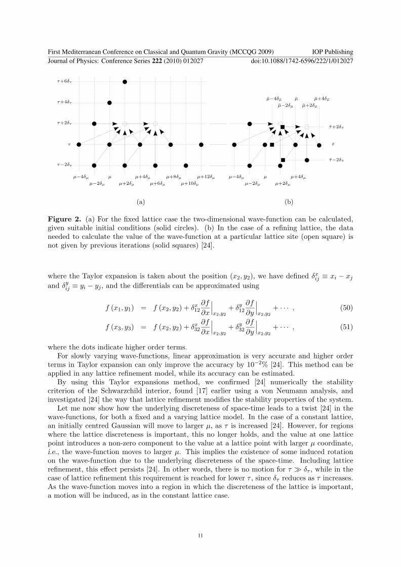
where δµ and δτ denote the step-sizes along the µ and τ directions, respectively.In the case of lattice refinement, δµ and δτ are decreasing functions of µ and τ , respectively,

and the data needed to calculate the value of the wave-function at a particular lattice site arenot given by previous iterations, as it is illustrated in Fig.2. We propose [24] to use Taylorexpansions to calculate the necessary data points. Let us assume that the matter Hamiltonianacts diagonally on the basis states of the wave-function, namely

Hφ|Ψ〉 ≡ Hφ

∑µ,τ

Ψµ,τ |µ, τ〉 =∑µ,τ

HφΨµ,τ |µ, τ〉 . (48)

Given a function evaluated at three (non-collinear) coordinates, the Taylor approximation tothe value at a fourth position is

f (x4, y4) = f (x2, y2) + δx42

∂f

∂x

∣∣∣x2,y2

+ δy42

∂f

∂y

∣∣∣x2,y2

+O(

(δx42)

2 ∂2f

∂x2

∣∣∣x2,y2

)+O

((δy

42)2 ∂2f

∂y2

∣∣∣x2,y2

), (49)


10

(a)

µ−4δµ µ µ+4δµ µ+8δµ µ+12δµ

µ−2δµ µ+2δµ µ+6δµ µ+10δµ

τ−2δτ

τ

τ+2δτ

τ+4δτ

τ+6δτ

(b)

µµ−4δµ µ+4δµ

µ−2δµ µ+2δµ

µ−4δµ

µ−2δµ

µ

µ+2δµ

µ+4δµ

τ

τ−2δτ

τ+2δτ

Figure 2. (a) For the fixed lattice case the two-dimensional wave-function can be calculated,given suitable initial conditions (solid circles). (b) In the case of a refining lattice, the dataneeded to calculate the value of the wave-function at a particular lattice site (open square) isnot given by previous iterations (solid squares) [24].

where the Taylor expansion is taken about the position (x2, y2), we have defined δxij ≡ xi − xj

and δyij ≡ yi − yj , and the differentials can be approximated using

f (x1, y1) = f (x2, y2) + δx12

∂f

∂x

∣∣∣x2,y2

+ δy12

∂f

∂y

∣∣∣x2,y2

+ · · · , (50)

f (x3, y3) = f (x2, y2) + δx32

∂f

∂x

∣∣∣x2,y2

+ δy32

∂f

∂y

∣∣∣x2,y2

+ · · · , (51)

where the dots indicate higher order terms.For slowly varying wave-functions, linear approximation is very accurate and higher order

terms in Taylor expansion can only improve the accuracy by 10−2% [24]. This method can beapplied in any lattice refinement model, while its accuracy can be estimated.

By using this Taylor expansions method, we confirmed [24] numerically the stabilitycriterion of the Schwarzchild interior, found [17] earlier using a von Neumann analysis, andinvestigated [24] the way that lattice refinement modifies the stability properties of the system.

Let me now show how the underlying discreteness of space-time leads to a twist [24] in thewave-functions, for both a fixed and a varying lattice model. In the case of a constant lattice,an initially centred Gaussian will move to larger µ, as τ is increased [24]. However, for regionswhere the lattice discreteness is important, this no longer holds, and the value at one latticepoint introduces a non-zero component to the value at a lattice point with larger µ coordinate,i.e., the wave-function moves to larger µ. This implies the existence of some induced rotationon the wave-function due to the underlying discreteness of the space-time. Including latticerefinement, this effect persists [24]. In other words, there is no motion for τ À δτ , while in thecase of lattice refinement this requirement is reached for lower τ , since δτ reduces as τ increases.As the wave-function moves into a region in which the discreteness of the lattice is important,a motion will be induced, as in the constant lattice case.


11

4. Anisotropic LQCVarious aspects of anisotropic cosmologies have been studied within LQC in the past [17, 25],however the first full and consistent quantisation of a Bianchi I cosmology (the simplest ofanisotropic cosmological models) was achieved recently in Ref. [26]. Moreover, the link backto the underlying full LQG theory has been strengthened, by considering the flux of the triadsthrough surfaces consistent with the Bianchi I anisotropic case. With the quantisation of theBianchi I model under control, it is possible to ask whether LQC features, obtained within thecontext of isotropic Friedmann-Lemaıtre-Roberston-Walker cosmology, are robust, at least withrespect to this limited extension of the symmetries of the system. Bianchi type I models, aparttheir simplicity, they present a particular interest for space-like singularities within the full LQGtheory. Following the same vein as for the isotropic case, a massless scalar field plays the role ofan internal time parameter. In the absence of such a field, physical evolution can be found byconstructing families of unitarily related partial observables, parametrised by geometry degreesof freedom [27].

4.1. Unstable Bianchi I LQCStudying stability conditions of the full Hamiltonian constraint equation describing the quantumdynamics of the diagonal Bianchi I model, I will show [28] that there is robust evidence of aninstability in the explicit implementation of the difference equation. On the one hand, such aresult may question the choice of the quantisation approach, the model of lattice refinement,and/or the role of ambiguity parameters. On the other hand, one may argue that such aninstability may not be necessarily a problem since it might be that unstable trajectories areexplicitly removed by the physical inner product.

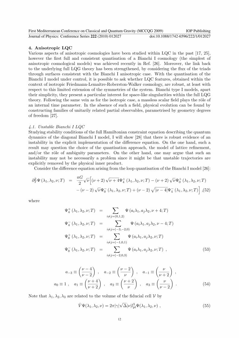
Consider the difference equation arising from the loop quantisation of the Bianchi I model [26]:

∂2T Ψ(λ1, λ2, ν;T ) =

πG

2√

ν[(ν + 2)

√ν + 4Ψ+

4 (λ1, λ2, ν; T )− (ν + 2)√

νΨ+0 (λ1, λ2, ν;T )

− (ν − 2)√

νΨ−0 (λ1, λ2, ν; T ) + (ν − 2)

√|ν − 4|Ψ−

4 (λ1, λ2, ν; T )]

,(52)

where

Ψ+4 (λ1, λ2, ν; T ) =

∑

i6=j=(0,1,2)

Ψ(aiλ1, ajλ2, ν + 4;T )

Ψ−4 (λ1, λ2, ν; T ) =

∑

i6=j=(−3,−2,0)

Ψ(aiλ1, ajλ2, ν − 4;T )

Ψ+0 (λ1, λ2, ν; T ) =

∑

i6=j=(−1,0,1)

Ψ(aiλ1, ajλ2, ν;T )

Ψ−0 (λ1, λ2, ν; T ) =

∑

i6=j=(−2,0,3)

Ψ(aiλ1, ajλ2, ν;T ) , (53)

a−3 ≡(

ν − 4ν − 2

), a−2 ≡

(ν − 2

ν

), a−1 ≡

(ν

ν + 2

),

a0 ≡ 1 , a1 ≡(

ν + 4ν + 2

), a2 ≡

(ν + 2

ν

), a3 ≡

(ν

ν − 2

). (54)

Note that λ1, λ2, λ3 are related to the volume of the fiducial cell V by

V Ψ(λ1, λ2, ν) = 2π|γ|√

∆|ν|l3plΨ(λ1, λ2, ν) , (55)


12

ν

λ1

λ2

λ1

a−2λ1

a−3λ1

λ2a−2λ2a

−3λ2

ν − 4

λ1

a−2λ1

a−1λ1

a−2λ2 a

−1λ2 λ2

λ1

a2λ1

a3λ1

λ2 a2λ2 a3λ2

ν

λ1

a1λ1

a2λ1

λ2 a1λ2 a2λ2

ν + 4

Figure 3. The geometry of the points used in the difference equation that results from theHamiltonian constraint, for the Bianchi I model [28].

with γ = sgn(p1p2p3)|γ| andν = 2λ1λ2λ3 , (56)

We will investigate the stability of the vacuum solutions, in which case the solution is static,namely Ψ (λ1, λ2, ν; T ) = Ψ (λ1, λ2, ν), simplifying considerably Eq. (52), whose geometry isdrawn in Fig. 3. To search for growing mode solutions we will perform a von Neumann analysis.In addition to specifying the boundary conditions on the ν and ν−4 planes, we are also requiredto specify the value at five of the points given in Ψ+

4 (λ1, λ2, ν). There are in total 23 valuesthat are required and with such initial data the difference equation, Eq. (52), can be used toevaluate the 24th point. Once this point has been evaluated, it can be used to move the centralpoint and evaluate the wave-function at subsequent positions in the ν + 4 plane.

Following the standard von Neumann stability analysis, we decompose the solutions of thedifference equation into Fourier modes and look for growing modes. Considering the ansatz [28]

Ψ (λ1, λ2, ν) = T (λ1) exp (i (ωλ2 + χν)) , (57)

where we have chosen the λ1 direction to be the direction in which the ν + 4 plane is evolved,


13

the difference equation becomes

e4χi∑

i6=j=(0,1,2)

T (aiλ1) ei(ωajλ2+χν) =√

ν

ν + 4

∑

i6=j=(−1,0,1)

T (aiλ1) ei(ωajλ2+χν)

+(

ν − 2ν + 2

) √ν

ν + 4

∑

i6=j=(−2,0,3)

T (aiλ1) ei(ωajλ2+χν)

−(

ν − 2ν + 2

) √|ν − 4|ν + 4

e−4χi∑

i6=j=(−3,−2,0)

T (aiλ1) ei(ωajλ2+χν) .

(58)

As it has been explicitly shown in Ref. [28], expanding in terms of small 1/ν, the differenceequation can be written in the form of a vector equation as

M1T 3 = M2T 2 , (59)

where we have defined the vectors

T i =

T (aiλ1)T (ai−1λ1)T (ai−2λ1)T (ai−3λ1)T (ai−4λ1)T (ai−5λ1)

for i = 2, 3 (60)

and the matrices

M1 =

A 0 0 0 0 00 1 0 0 0 00 0 1 0 0 00 0 0 1 0 00 0 0 0 1 00 0 0 0 0 1

, M2 =

B C D E F G1 0 0 0 0 00 1 0 0 0 00 0 1 0 0 00 0 0 1 0 00 0 0 0 1 0

. (61)

The condition for stability can be written as follows: If

max |λ| ≤ 1 ∀ ω and χ , (62)

where λ are the eigenvalues of the matrix (M1)−1 M2, the amplitude T (a3λ1) is less than that

of previous points, in other words, the difference equation is stable. Let us define the parameterΛ = ωλ2/ν. The presence of an instability in the difference equation has been demonstrated [28]in several ways: (i) there is a particular set of critical modes, Λ = (2n − 1)π/2, with n ∈ Z,for which the system is unstable; (ii) in the large ν limit, the system is unstable for the modesΛ = π/4 and χ = 0; (iii) the system is unstable for a general ν, for modes that approach thecritical value.

In conclusion, the difference equation, Eq. (52), is unconditionally unstable, in the sense thatthere is no region of (λ1, λ2, ν) in which Eq. (52) is stable.


14

4.2. Lattice refinement from isotropic embedding of anisotropic cosmologyGiven a consistent quantum anisotropic model, one can find [29] isotropic states for which thediscrete step-size of the isotropically embedded Hamiltonian constraint is not necessarily thatof the p−1/2 (new quantisation) step-size. The choice of different embeddings has importantconsequences for the precise form of discretisation in the isotropic sub-system. In this sense,lattice refinement could be interpreted as being due to the degrees of freedom that are absentin the isotropic model [29].

In the standard approach, isotropic states are taken to be those in which the three scalefactors are λ1 = λ2 = λ3, or more precisely, defining the volume of the state as ν = 2λ1λ2λ3 toeliminate one of the directions (λ3), the map

|Ψ(λ1, λ2, ν)〉 →∣∣∣

∑

λ1,λ2

Ψ(λ1, λ2, ν)〉 ≡ |Ψ(ν)〉 , (63)

produces isotropic states. Working with the three scale factors λi, one can show [29] that thereis an ambiguity in exactly what the volume of such an isotropic state is. Consider the state

|Ψ (λ1, λ2, λ3)〉 ≡ 1A

[|Ψ(λ1, λ2, λ3)〉+ |Ψ(λ3, λ1, λ2)〉+ |Ψ (λ2, λ3, λ1)〉

], (64)

with the restriction

〈Ψ(λ1, λ2, λ3) |Ψ (λ3, λ1, λ2)〉 = 〈Ψ (λ1, λ2, λ3) |Ψ(λ2, λ3, λ1)〉 = 〈Ψ(λ3, λ1, λ2) |Ψ(λ2, λ3, λ1)〉 ,

on the anisotropic states. The expectation values of the scale factors along each direction ofsuch a state are

〈λi〉 =λ1 + λ2 + λ3

3. (65)

The measured scale factor is equal in each direction and is given by the average of the scalefactors of the underlying, anisotropic states. However, the measured volume of such a state is justν = 2λ1λ2λ3, which is not the cube of the measured scale factor. Thus, while it is the eigenvalueof the anisotropically defined volume operator, it is not necessarily what we would measure as thevolume. Essentially, the reason for this is that while the scale factors λi are measured to be equalin each direction, they are not eigenvalues of the state, i.e., λi|Ψ (λ1, λ2, λ3)〉 6= λi|Ψ (λ1, λ2, λ3)〉.However, both the average and the product (i.e., the volume) of the scale factors are eigenvalues.It is this ambiguity, that leads to the possibility of deviations from the standard isotropic case.

In conclusion, the difference between the two procedures is essentially due to what oneconsiders to be more fundamental, the volume of the underlying states (ν) or the measuredvolume of the symmetric state (〈λ〉3), which are not necessarily equal. Choosing ν leads to thenew quantised Hamiltonian of isotropic cosmology, while choosing 〈λ〉3 results in some kind ofdifferent lattice refinement. This lattice refinement is significantly more complicated that thesingle power law behaviour, pA, usually considered.

5. ConclusionsLoop Quantum Gravity proposes a method of quantising gravity in a background independent,non-perturbative way. Quantum gravity is essential when curvature becomes large, as forexample in the early stages of the evolution of the universe. Applying LQG in a cosmologicalcontext leads to Loop Quantum Cosmology which is a symmetry reduction of the infinitedimensional phase space of the full theory, allowing us to study certain aspects of the theoryanalytically. The discreteness of spatial geometry, a key element of the full theory, leads tosuccesses in LQC which do not hold in the Wheeler-de Witt quantum cosmology.

By studying phenomenological consequences of LQC we can get some useful insight about thefull LQG theory and get an answer to some long-standing questions in early universe cosmology.Here, I have briefly described some of the phenomenological aspects of LQC.


15

AcknowledgmentsIt is a pleasure to thank the organisers of the First Mediterranean Conference on Classical andQuantum Gravity (MCCQG) (http://www.phy.olemiss.edu/mccqg/), for inviting me to givethis talk, in the beautiful island of Crete in Greece. This work is partially supported by theEuropean Union through the Marie Curie Research and Training Network UniverseNet (MRTN-CT-2006-035863).

References[1] Guth A 1981 Phys. Rev. D 23 347[2] Sakellariadou M 2008 Lect. Notes Phys. 738 359[3] Piran T 1986 Phys. Lett. B 181 238[4] Goldwirth D 1991 Phys. Rev. D 43 3204[5] Calzetta E and Sakellariadou M 1992 Phys. Rev. D 45 2802[6] Calzetta E and Sakellariadou M 1993 Phys. Rev. D 47 3184[7] Germani C, Nelson W and Sakellariadou M 2007 Phys. Rev. D 76 043529[8] Gibbons G and Turok N 2008 Phys. Rev. D 77 063516[9] Ashtekar A and Sloan D 2009 Loop quantum cosmology and slow roll inflation (Preprint 0912.4093)[10] Rovelli C 2004 Quantum Gravity (Cambridge: Cambridge University Press)[11] Thiemann T 2007 Modern Canonical Quantum General Relativity (Cambridge: Cambridge University Press)[12] Bojowald M 2005 Living Rev. Rel. 8 11[13] Ashtekar A and Lewandowski J 1997 Class. & Quant. Grav. 14 A55[14] Ashtekar A, Pawlowski T and Singh P 2006 Phys. Rev. D 74 084003[15] Vandersloot K 2005 Phys. Rev. D 71 103506[16] Rosen J, Jung J H and Khanna G 2006 Class. Quant. Grav. 23 7075[17] Bojowald M, Cartin D and Khanna G 2007 Phys. Rev. D 76 064018[18] Sakellariadou M 2009 J. Phys. Conf. Ser. 189 012035[19] Nelson W and Sakellariadou M (2007) Phys. Rev. D 76 104003[20] Nelson W and Sakellariadou M 2007 Phys. Rev. D 76 044015[21] Corichi A and Singh P 2008 Phys. Rev. D 78 024034[22] Nelson W and Sakellariadou M 2008 Phys. Rev. D 78 024006[23] Ashtekar A, Pawlowski T and Singh P 2006 Phys. Rev. D 74, 084003[24] Nelson W and Sakellariadou M 2008 Phys. Rev. D 78 024030[25] Chiou D W and Vandersloot K 2007 Phys. Rev. D 76 084015[26] Ashtekar A and Wilson-Ewing E 2009 Phys. Rev. D 79 083535[27] Martin-Benito M, Mena Marugan G A and Pawlowski T 2009 Phys. Rev. D 80 084038[28] Nelson W and Sakellariadou M 2009 Phys. Rev. D 80 063521[29] Nelson W and Sakellariadou M 2009 Lattice Refining Loop Quantum Cosmology from an Isotropic Embedding

of Anisotropic Cosmology (Preprint 0906.0292)


16

Date post:	27-Jan-2017
Category:	Documents
Upload:	mairi
View:	212 times
Download:	0 times

Phenomenology of loop quantum cosmology

Documents