Phonetic- and Speaker-Discriminant Features for Speaker Recognition by Lara Stoll Research Project Submitted to the Department of Electrical Engineering and Computer Sciences, University of California at Berkeley, in partial satisfaction of the requirements for the degree of Master of Science, Plan II. Approval for the Report and Comprehensive Examination: Committee: Professor Nelson Morgan Research Advisor Date ****** Dr. Nikki Mirghafori Second Reader Date
Transcript
Phonetic- and Speaker-Discriminant Features for Speaker Recognition
by Lara Stoll
Research Project
Submitted to the Department of Electrical Engineering and Computer Sciences, University ofCalifornia at Berkeley, in partial satisfaction of the requirements for the degree of Master ofScience, Plan II.
Approval for the Report and Comprehensive Examination:
5.17 DET curves for the Speaker-SVM systems using different numbers of Speaker-MLPtraining speakers . . . . . . . . . . . . . . . . . . . . . . . . . . . . . . . . . . . . . . 37
5.18 DET curves for Speaker-SVM combination with Basic-GMM . . . . . . . . . . . . . 39
5.19 DET curves for Speaker-SVM combination with SRI-GMM . . . . . . . . . . . . . . 39
5.20 DET curves for Basic-GMM, Speaker-SVM and their score-level combination, undermatched and mismatched conditions . . . . . . . . . . . . . . . . . . . . . . . . . . . 41
5.21 DET curves for SRI-GMM, Speaker-SVM and their score-level combination, undermatched and mismatched conditions . . . . . . . . . . . . . . . . . . . . . . . . . . . 41
iv
List of Tables
5.1 Tandem/HATS-GMM system improves upon Basic-GMM system, especially in com-bination, but there is no improvement for SRI-GMM system. . . . . . . . . . . . . . 25
5.2 Fusion results with the Tandem/HATS-GMM system for both matched and mis-matched conditions show improvements for the Basic-GMM, but no change for theSRI-GMM. . . . . . . . . . . . . . . . . . . . . . . . . . . . . . . . . . . . . . . . . . 27
5.3 Tandem-GMM system yields improvements over the Basic-GMM system, especiallyin combination, but none for the SRI-GMM system. . . . . . . . . . . . . . . . . . . 29
5.4 Fusion results with the Tandem-GMM system show improvements for the Basic-GMM, especially for the mismatched case, but only improvements in the matchedcondition for the SRI-GMM. . . . . . . . . . . . . . . . . . . . . . . . . . . . . . . . . 32
5.5 HATS-GMM system results show gains for combination with the Basic-GMM, butnone for fusion with the SRI-GMM. . . . . . . . . . . . . . . . . . . . . . . . . . . . 32
5.6 Fusion results with the HATS-GMM system show improvements in the matched andmismatched cases for the Basic-GMM, but only improvement in the matched casefor the SRI-GMM. . . . . . . . . . . . . . . . . . . . . . . . . . . . . . . . . . . . . . 34
5.7 CV accuracy improves as the number of hidden units increase. . . . . . . . . . . . . 36
5.8 Speaker-SVM results improve as the number of hidden units increase. . . . . . . . . 37
5.9 System combination with 64 speaker, 1000 hidden unit Speaker-SVM improves Basic-GMM results, but not the SRI-GMM. . . . . . . . . . . . . . . . . . . . . . . . . . . 38
5.10 Fusion results with the Speaker-SVM system for both matched and mismatchedconditions show improvement for the Basic-GMM, but virtually no change for theSRI-GMM. . . . . . . . . . . . . . . . . . . . . . . . . . . . . . . . . . . . . . . . . . 38
6.1 Results for the MLP-based systems and their feature-level and score-level combina-tions with the Basic-GMM. . . . . . . . . . . . . . . . . . . . . . . . . . . . . . . . . 43
6.2 Results for the MLP-based systems and their score-level combinations with the SRI-GMM. . . . . . . . . . . . . . . . . . . . . . . . . . . . . . . . . . . . . . . . . . . . . 43
6.3 Breakdown of results for matched and mismatched conditions for the MLP-basedsystems and their score-level fusions with the Basic-GMM. . . . . . . . . . . . . . . . 44
v
6.4 Breakdown of results for matched and mismatched conditions for the MLP-basedsystems and their score-level fusions with the SRI-GMM. . . . . . . . . . . . . . . . 44
vi
Acknowledgements
First and foremost, I would like to thank Joe Frankel and Nikki Mirghafori, who collaboratedwith me on this work. Joe’s contributions and enthusiasm for the project and Nikki’s suggestionsand insight were both invaluable and much appreciated. I also want to extend my gratitude tomy official research advisor, Professor Nelson Morgan, who allowed me to join the speech groupat the International Computer Science Institute (ICSI), and who has provided me with a usefulperspective on my project work. For their support and helpful comments, I thank the speakerrecognition group at ICSI, including George Doddington, Andy Hatch, Howard Lei, Mary Knox,and Christian Mueller. Additional thanks go to Sachin Kajarekar and Andreas Stolcke of SRI, whoprovided technical expertise for my system implementation.
This work was supported by a National Science Foundation Graduate Research Fellowship, andby a UC-Berkeley Graduate Research Opportunity Fellowship.
vii
Chapter 1
Introduction
The speaker recognition task is that of deciding whether or not a new test utterance belongsto a given target speaker, for whom there is only a limited amount of training data available. Thetraditionally successful approach to speaker recognition involves using low-level cepstral featuresextracted from speech in a Gaussian mixture model (GMM) system [2]. Alternative approachesattempt to make use of so-called high-level features, which involve, for instance, prosody and wordusage [3]; however, the systems using low-level features are still the best base system, as the con-tribution of high-level approaches generally comes in combination with an approach using low-levelfeatures.
We, as humans, are able to recognize a speaker’s identity when we hear him speak, providedthat the speaker is known to us, that is, we have heard enough of his speech. While a humansystem is able to extract the information necessary to identify a speaker under a wide range ofconditions, it is a significant challenge for an automatic speaker recognition system to extract in-formation from the speech in a meaningful way. Although cepstral features have proven to be themost successful choice of low-level features for speech processing, discriminatively trained featuresin a speaker space may be better suited to the speaker recognition problem. Accordingly, the focusof this report is on the development of low-level features specifically designed for use in the task ofspeaker recognition.
The approach taken in this report utilizes multi-layer perceptrons (MLPs) as a means of per-forming a feature transformation of cepstral features. A comparison is made between using MLPnetworks trained to discriminate between phones and using MLPs trained to discriminate betweenspeakers. In the former case, Tandem/HATS features, originally developed at ICSI for speechrecognition, are tested in a GMM speaker recognition system. In the latter case, 3-layer MLPs ofdifferent sizes, that is, with varying numbers of hidden units, are trained to distinguish betweena set of output speakers; several sizes of training speaker sets are considered as well. Then, thehidden activations of the Speaker-MLPs are tested as features in a support vector machine (SVM)system.
The basic motivation behind testing the Tandem/HATS features in a speaker recognition sys-tem is to determine whether or not the inclusion of longer-term (i.e., around 500ms) phonetic
1
information is able to aid in distinguishing between speakers. Although these phonetic featureshave been able to improve speech recognition systems, and other speaker recognition systems havebeen successful in utilizing phonetic content, to the best of my knowledge, the Tandem/HATSfeatures have never been tested in a speaker recognition task. By training the Speaker-MLPs todiscriminate between speakers, the features they produce should, by design, be speaker discrimi-native, and thus well-suited to speaker recognition. Although similar speaker-discriminative MLPwork has been done, the Speaker-MLPs of this report experiment with larger network topologieswith the idea that increasing the number of training speakers and size of the network may yieldadditional improvements in performance.
The report begins with background material relevant to speaker recognition, including a de-scription of the task, cepstral features, GMM and SVM systems, and various normalizations, inChapter 2. A discussion of research related to a discriminant feature approach follows in Chapter3, including work done in developing phonetically discriminative and speaker discriminative fea-tures, some of which also involves the use of MLPs. Chapter 4 explains this report’s approach andmethodology to the feature generation and usage, including the motivation, detailed descriptionsof the Tandem/HATS MLP features and Speaker-MLP features, baseline systems, and how thesystems are combined. Chapter 5 outlines the data used for training and testing, the performancemeasures presented, the experimental setup, and the results of the experiments. Finally, the reportends with conclusions in Chapter 6.
2
Chapter 2
Background
In order to provide a framework of relevant information, this chapter presents a brief overviewof topics related to speaker recognition. The basic knowledge given here will be assumed for theremainder of the report. To begin, the characteristics of the speaker recognition problem aredescribed in Section 2.1.
2.1 The Speaker Recognition Problem
As its name implies, automatic speaker recognition attempts to recognize, or identify, a givenspeaker by processing his/her speech automatically, that is to say, in a fully objective and reprod-ucable manner, without the aid of human listening. In order to be able to recognize the speaker ofa given test utterance, it is necessary to have training data first, so that the system can “learn” thespeaker(s) of interest. The term speaker recognition can be used to refer to a variety of tasks. Onetype of task is speaker identification, when the system must produce the identity of the speaker,given a test utterance, from a set of speakers. With closed-set speaker identification, the number ofspeakers in the set is fixed, and the system must choose which among the given speakers is a matchto the speaker of the test utterance. Open-set speaker identification adds a layer of complexityby allowing the test utterance to belong to a speaker not in the set of speakers for whom there istraining data available. A second type of task is speaker verification, which involves a hypotheticaltarget speaker match to the test speaker, and the system must determine whether or not the testspeaker identity is as claimed.
Regardless of which type of task, the problem may be further characterized as being text-dependent or text-independent. In the text-dependent case, the train and test utterances arerequired to be a specific word or set of words; the system can then exploit the knowledge of what isspoken in order to better make a decision. For the text-independent case, there is no constraint onwhat is said in the speech utterances, allowing for generalization to a wider variety of situations.
This report focuses on the text-independent speaker verification task. For each target, or hy-
3
pothesis, speaker and test utterance pair, the system must decide whether or not the speakeridentities are the same. In this case, two types of errors arise: false acceptance, or false alarm,and false rejection, or missed detection. A false accept occurs when the system incorrectly verifiesan impostor test speaker as the target speaker. A false reject occurs when the system incorrectlyidentifies the test speaker as an impostor speaker.
In order to perform a speaker recognition task, the system must first parameterize the speechin a meaningful way that will allow the system to distinguish and characterize speakers and theirspeech; this step is addressed in Section 2.2, which discusses two types of cepstral features com-monly used in speech processing applications. For speaker verification, which is essentially a binarydecision task, a statistical framework is utilized in the following way. Models are trained for boththe target speaker, using the training data, as well as for a background speaker model, using sep-arate data from a large number of speakers, representative of some generic speaker. Then, theprobability of the test utterance is determined for each model, and a score relating to the likelihoodratio of the probabilities of the test utterance given each model is produced. Two commonly usedapproaches to the statistical modeling, Gaussian mixture models and support vector machines, arediscussed in Section 2.3.
Although there are many additional issues that arise in the area of speaker recognition, thisreport will only consider one more type of difficulty, that of channel mismatch. Since the speakerrecognition system directly uses the speech signal, in parameterized form, variations in the signaldue to channel type or noise can significantly impact performance of the system. If there is achannel mismatch between the training and test data, i.e., if they were recorded on different chan-nels, then the system may falsely reject a true target speaker match because the data “appears” tobelong to a different speaker because of the channel variation. Normalizations developed to addresssuch a channel issue are discussed in Section 2.4. These include normalizations that are applied onthe score-level, the feature-level, and the model-level.
2.2 Cepstral Features
The process of parameterizing speech is referred to as feature extraction. Low-level featuresare those based directly on frames of the speech signal, where a frame refers to a window that istypically 25 ms long. High-level features, on the other hand, incorporate information from morethan just one frame of speech, and include, for example, speaker idiosyncrasies, prosodic patterns,pronunciation patterns, and word usage. There are two types of low-level cepstral features relevantto this report, and they are explained here.
Mel-frequency cepstral coefficients, or MFCCs, are generated by the process shown in Figure2.1. First, an optional preemphasis filter is applied, to enhance the higher spectral frequencies andcompensate for the unequal perception of loudness at different frequencies. Next, the speech signalis windowed into 20-30ms frames (with 10ms overlap) and the absolute value of the fast Fouriertransform (FFT) is calculated for each frame. A Mel-frequency triangular filterbank is then applied,where the Mel scale is an auditory scale based on pitch perception. The Mel frequency is relatedto the linear frequency scale by
fMel = 1127 ·log(1 + flinear
700 )log2
(2.1)
4
For this work, the number of filters is 24. After the spectrum has been smoothed, the log is taken.Finally, a discrete cosine transform (DCT) is applied to obtain the cepstral coefficients, cn:
cn =K∑
k=1
Sk cos[n(k − 1
2)π
K
], n = 1, 2, . . . , L (2.2)
where Sk are the log-spectral vectors from the previous step, K is the total number of log-spectralcoefficients, and L is the number of coefficients to be kept (this is called the order of the MFCCs),with L ≤ K.
Pre−emphasis
filterWindow FFT | |
Speech
signal Filterbank
Mel−frequencyLog
Cepstral
coefficientsDCT
Figure 2.1. Generation of MFCC features
Perceptual linear prediction coefficients, or PLPs, are based on linear predictive coding, andare quite similar to MFCCs. The process of generating PLPs is shown in Figure 2.2. First, thespeech signal is windowed, as before, into 20-30ms frames with 10ms overlap, and the magnitudeof the FFT is calculated. Then, a filterbank is applied, this time using trapezoidally shaped filterson a Bark scale, where
Next is the pre-emphasis step, which is done by weighting the spectrum with an equal loudnesscurve, which again emphasizes the higher frequencies. Instead of taking the log, as in the MFCCcase, the cube root is taken, as an approximation to the power-law of hearing that relates intensityto loudness. As with MFCCs, the inverse DFT is taken; in the PLP case, the results are not cepstralcoefficients, but are instead similar to autocorrelation coefficients. Next, the compressed spectrumis smoothed using an autogressive model. Finally, the autoregressive coefficients are converted tocepstral coefficients.
In addition to using the MFCCs or PLPs, it is common to include estimates of their first, second,and possibly third derivatives as additional features. These are referred to as deltas, double-deltas,and triple-deltas. The polynomial approximations of the first and second derivatives are as follows:
5
∆cm =∑l
k=−l kcm+k∑lk=−l|k|
∆∆cm =∑l
k=−l k2cm+k∑l
k=−l k2
(2.4)
Furthermore, an energy term and/or its derivative can also be included in the feature parameteri-zation.
2.3 System Approaches
2.3.1 Gaussian Mixture Model (GMM)
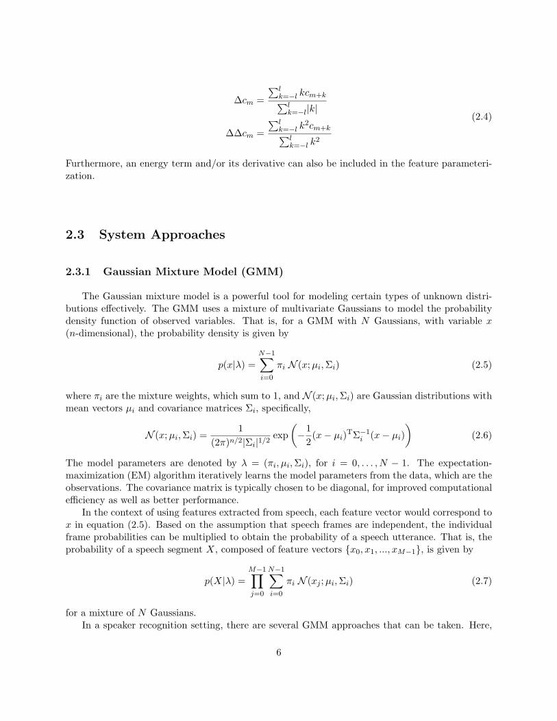
The Gaussian mixture model is a powerful tool for modeling certain types of unknown distri-butions effectively. The GMM uses a mixture of multivariate Gaussians to model the probabilitydensity function of observed variables. That is, for a GMM with N Gaussians, with variable x(n-dimensional), the probability density is given by
p(x|λ) =N−1∑i=0
πi N (x;µi,Σi) (2.5)
where πi are the mixture weights, which sum to 1, and N (x;µi,Σi) are Gaussian distributions withmean vectors µi and covariance matrices Σi, specifically,
N (x;µi,Σi) =1
(2π)n/2|Σi|1/2exp
(−1
2(x− µi)TΣ−1
i (x− µi))
(2.6)
The model parameters are denoted by λ = (πi, µi,Σi), for i = 0, . . . , N − 1. The expectation-maximization (EM) algorithm iteratively learns the model parameters from the data, which are theobservations. The covariance matrix is typically chosen to be diagonal, for improved computationalefficiency as well as better performance.
In the context of using features extracted from speech, each feature vector would correspond tox in equation (2.5). Based on the assumption that speech frames are independent, the individualframe probabilities can be multiplied to obtain the probability of a speech utterance. That is, theprobability of a speech segment X, composed of feature vectors {x0, x1, ..., xM−1}, is given by
p(X|λ) =M−1∏j=0
N−1∑i=0
πi N (xj ;µi,Σi) (2.7)
for a mixture of N Gaussians.In a speaker recognition setting, there are several GMM approaches that can be taken. Here,
6
only the currently prevalent approach is described, for which two GMM models are needed: onefor the target speaker and one for the background model [2]. Using training data from a largenumber of speakers, a speaker-independent universal background model, or UBM, is generated.So that every target speaker model is in the same space and can be compared to one another,the speaker-dependent models are adapted from the UBM using maximum a posteriori (MAP)adaptation. For a given test utterance X, and a given target speaker, a log likelihood ratio (LLR)can then be calculated:
LLR(X) = log p (X|λtarget)− log p (X|λUBM ) (2.8)
Comparing the LLR to a threshold, Θ, will determine the decision made about the test speaker’sidentity: if LLR(X) > Θ, the test speaker is identified as a true speaker match, otherwise, the testspeaker is determined to be an impostor.
2.3.2 Support Vector Machine (SVM)
Support vector machines, or SVMs, are a supervised learning method that can be used forpattern classification problems [4]. For binary classification, which is the task of interest here,the SVM is a linear classifier that finds a separating hyperplane between data points in each class.Furthermore, the SVM learns the maximum-margin hyperplane that will separate the data, makingit a maximum-margin classifier. In this case, the “model” for each target speaker is the defininghyperplane, and instead of probabilities for data given a distribution, distances from the hyperplaneare used.
In mathematical terms, the SVM problem can be formulated as
min ‖w‖2 + C∑
i
ξi
subject to yi(w · xi − b) ≥ 1− ξi, 1 ≤ i ≤ n
(2.9)
where ξi are slack variables, xi are the training data points, yi are the corresponding class labels(+1 or −1), C is a constant, and w and b are the hyperplane parameters. Essentially, the goal isto find the hyperplane such that sign(w · xi − b) = yi, up to some soft margin involving ξi.
The SVM is used in speaker recognition by taking one or more positive examples of the targetspeaker, as well as a set of negative examples of impostor speakers, and producing a hyperplanedecision boundary. Since there are far more impostor speaker examples than target speaker exam-ples, a weighting factor is used to make the target example(s) count as much as all of the impostorexamples. Once the hyperplane for a given target speaker is known, the test speaker can be classi-fied as belonging to either the target speaker or impostor speaker class. Instead of a log likelihoodratio, a score can be produced by using the distance of the test data from the hyperplane boundary.
7
2.4 Normalizations
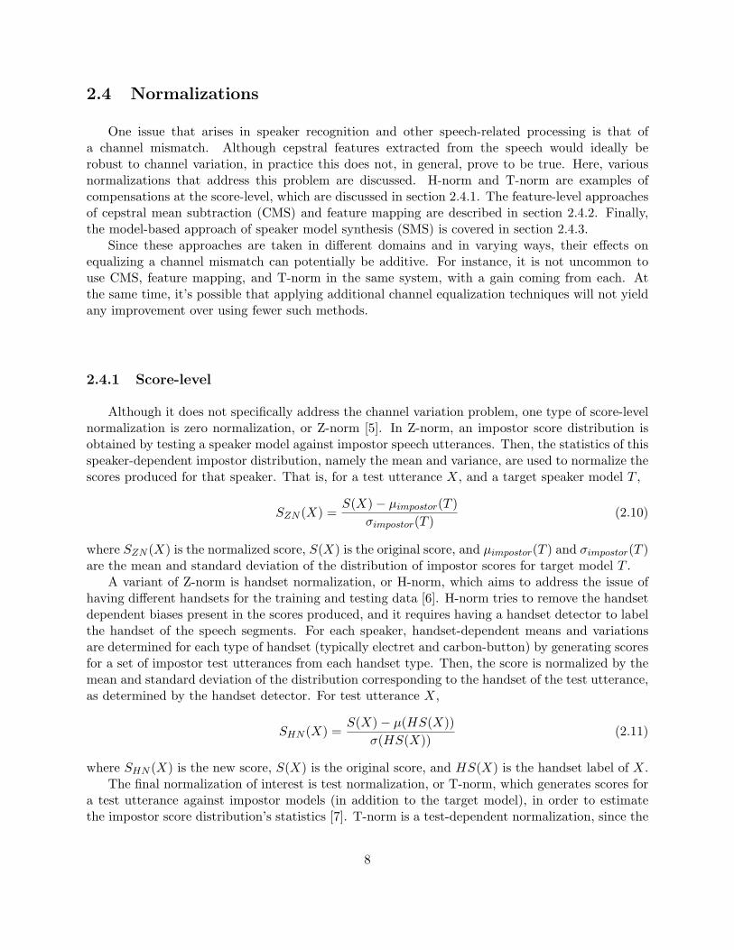
One issue that arises in speaker recognition and other speech-related processing is that ofa channel mismatch. Although cepstral features extracted from the speech would ideally berobust to channel variation, in practice this does not, in general, prove to be true. Here, variousnormalizations that address this problem are discussed. H-norm and T-norm are examples ofcompensations at the score-level, which are discussed in section 2.4.1. The feature-level approachesof cepstral mean subtraction (CMS) and feature mapping are described in section 2.4.2. Finally,the model-based approach of speaker model synthesis (SMS) is covered in section 2.4.3.
Since these approaches are taken in different domains and in varying ways, their effects onequalizing a channel mismatch can potentially be additive. For instance, it is not uncommon touse CMS, feature mapping, and T-norm in the same system, with a gain coming from each. Atthe same time, it’s possible that applying additional channel equalization techniques will not yieldany improvement over using fewer such methods.
2.4.1 Score-level
Although it does not specifically address the channel variation problem, one type of score-levelnormalization is zero normalization, or Z-norm [5]. In Z-norm, an impostor score distribution isobtained by testing a speaker model against impostor speech utterances. Then, the statistics of thisspeaker-dependent impostor distribution, namely the mean and variance, are used to normalize thescores produced for that speaker. That is, for a test utterance X, and a target speaker model T ,
SZN (X) =S(X)− µimpostor(T )
σimpostor(T )(2.10)
where SZN (X) is the normalized score, S(X) is the original score, and µimpostor(T ) and σimpostor(T )are the mean and standard deviation of the distribution of impostor scores for target model T .
A variant of Z-norm is handset normalization, or H-norm, which aims to address the issue ofhaving different handsets for the training and testing data [6]. H-norm tries to remove the handsetdependent biases present in the scores produced, and it requires having a handset detector to labelthe handset of the speech segments. For each speaker, handset-dependent means and variationsare determined for each type of handset (typically electret and carbon-button) by generating scoresfor a set of impostor test utterances from each handset type. Then, the score is normalized by themean and standard deviation of the distribution corresponding to the handset of the test utterance,as determined by the handset detector. For test utterance X,
SHN (X) =S(X)− µ(HS(X))
σ(HS(X))(2.11)
where SHN (X) is the new score, S(X) is the original score, and HS(X) is the handset label of X.The final normalization of interest is test normalization, or T-norm, which generates scores for
a test utterance against impostor models (in addition to the target model), in order to estimatethe impostor score distribution’s statistics [7]. T-norm is a test-dependent normalization, since the
8
same test utterance is used for testing and for generating normalization parameter estimates. Inmathematical terms,
STN (X) =S(X)− µimpostor(X)
σimpostor(X)(2.12)
where STN (X) is the normalized score, S(X) is the original score, and µimpostor(X) and σimpostor(X)are the mean and standard deviation of the distribution of scores for test utterance X against theset of impostor speaker models.
2.4.2 Feature-level
Cepstral mean subtraction (CMS) is a fairly simple technique that is applied at the feature-level [8]. CMS subtracts the time average from the output cepstrum in order to produce a zeromean log cepstrum. That is, for a temporal sequence of each cepstral coefficient cm,
cm(t) = cm(t)− 1T
T∑τ=1
cm(τ) (2.13)
The purpose of CMS is to remove the effects of the transmission channel, yielding improvedrobustness. However, any non-linear channel effects will remain, as will any time-varying linearchannel effects. Furthermore, CMS can remove some of the speaker characteristics, as the averagecepstrum does contain speaker-specific information.
Another feature-level channel compensation method is feature mapping [9]. Feature mappingaims to map features from different channels into the same channel-independent feature space. Achannel-independent root GMM is trained, and channel-dependent background GMMs are adaptedfrom the root. Feature-mapping functions are obtained from the model parameter changes betweenthe channel-independent and channel-dependent models. The most likely channel is detected forthe speaker data, which is then mapped to the channel-independent space. Adaptation to targetspeaker models is done using mapped features, and during verification, the mapped features ofthe test utterance are used for scoring. The root GMM is used as the UBM for calculating the loglikelihood ratios.
2.4.3 Model-level
Speaker model synthesis (SMS) is a model-based technique that utilizes channel-dependentmodels [10]. Rather than having one speaker-independent UBM, the SMS approach begins witha channel- and gender-independent root model, and then uses Bayesian adaptation to obtainchannel- and gender-dependent background models. Channel-specific target speaker modelsare also adapted from the appropriate background model, after the gender and channel of thetarget speaker’s training data have been detected. Furthermore, a transformation for each pairof channels is calculated using the channel-dependent background models; this transformationmaps the weights, means, and variances of a channel a model to the corresponding parametersof a channel b model. During testing, if the detected channel of the test utterance matches
9
the type of channel of the target speaker model, then that speaker model and the appropriatechannel-dependent background model are used to calculate the LLR for that test utterance.On the other hand, if the detected channel of the test utterance is not a match to the tar-get speaker model, then a new speaker model is synthesized using the previously calculatedtransformation between the target and test channels. Then, the synthesized model and the corre-sponding channel-dependent background model are used to calculate the LLR for the test utterance.
10
Chapter 3
Related Work
In speech processing applications, the development of discriminant features typically involvesdiscrimination based on either phones or speakers, i.e., the transformation or projection of featuresinto either a phonetic or a speaker space. There are also some approaches that cannot be identifiedas involving just one or the other, but are rather a mixture incorporating both phone and speakerspaces. This chapter outlines the prior work most related to the approach taken in this report.
3.1 Phonetically Discriminative Features
The use of features generated by a MLP (or possibly MLPs) trained to distinguish betweenphones has been shown to improve performance for automatic speech recognition (ASR). Re-searchers at ICSI developed Tandem/HATS-MLP features, which incorporate longer term temporalinformation through the use of MLPs whose outputs are phone posteriors [1, 11–14]. The Tandemcomponent of the features is generated using a 3-layer MLP, which takes as input 9 frames ofperceptual linear prediction (PLP) features, with deltas and double-deltas (about 200 ms), trainedto output 46 phone posteriors. The HATS, or Hidden Activation TempoRAl PatternS, componentinvolves two stages of MLPs. The first stage is a set of MLPs, one for each critical frequencyband, which each take as input 500 ms of critical band energies, and are each trained to output 46phone posteriors; the hidden activation outputs of these MLPs are then joined using the secondstage MLP. Finally, the Tandem and HATS phone posteriors are merged using a weighted average,and further transformed by log, principal component analysis (PCA), and truncation to producethe final features. For the Large Vocabulary Conversational Speech Recognition (LVCSR) of theNIST 2001 Hub-5 test set, augmenting PLPs with the Tandem/HATS MLP features yielded a10% relative error reduction over a PLP baseline [12]. For the 2004 Rich Transcription evaluation,a system using MFCCs augmented with the Tandem/HATS MLP features yields a 9.9% relative
11
improvement over a baseline system that uses MFCC and PLP features [13].
3.2 Speaker Discriminative Features
3.2.1 Using Neural Networks
The work most directly related to my own also uses artificial neural networks (ANN) trainedto perform speaker discrimination. Heck and Konig, et al., focused on extracting speaker discrimi-native features from Mel-frequency cepstral coefficents (MFCCs) using a MLP [15, 16]. A 5-layerMLP was trained to discriminate between 31 speakers; features were then extracted by taking the34 outputs from the third, bottleneck layer of the MLP for use in a GMM speaker recognitionsystem. The input to the MLP consisted of 9 frames of 17th order MFCCs and an estimate ofpitch. A comparison of frame-level cross-validation results, which were found to correlate stronglyto the results of the complete speaker verification system, i.e., the results when using the featuresin a GMM system, showed that 9 frames of MFCCs performed better than just 1 frame, and thatthe inclusion of pitch as an input also improved performance. Furthermore, the MLP features,when combined on the score-level with a cepstral only system, yielded consistent improvementwhen the training data and testing data were collected from mismatched telephone handsets [15].
In a similar approach, Morris and Wu, et al., generated MLP-based features for speakeridentication experiments [17–19]. However, in addition to the 5-layer MLP topology, they alsotested 3-layer and 4-layer MLPs, finding that features taken from the net-input values to thesecond hidden layer of the 5-layer MLP performed the best [18]; for each network topology, thedimension of the bottleneck hidden layer (from which the features were obtained) was 19, the sameas the number of inputs, while the other hidden layers used 100 units. The issue of selecting abasis of speakers to use for training the MLP was also addressed by Morris et al., who concludedthat a Maximum Average Distance method of speaker basis selection, where the distance is anestimate of the Kullback-Leibler distance, worked best [18]. Speaker identification performancealso improved as more speakers were used to train the MLP, up to a certain limit [17,19].
3.2.2 Using a Speaker Space
For the tasks of speaker recognition and identification, several methods specifically consider aspeaker space. Sturim, et al. utilized anchor models in order to create a characterization vector,where each component is a likelihood score from one of N pre-trained anchor models, for eachspeech utterance [20]. A vector distance between two characterization vectors, which are essentiallyprojections of the speech utterance into a speaker space, could then be used to compare a targetspeaker’s speech segment with an unknown speaker’s speech segment. When testing the anchorsystem in a speaker detection task, they found that the baseline GMM system had significantlybetter performance than the anchor system. However, when considering a Speaker Indexing task,
12
the computational efficiency of the anchor model system provided an advantage.Mami and Charlet used a similar anchor model approach, with certain modifications. They
found that using the angle between coordinate vectors of speakers yielded better results thanusing the distance between the vectors, and that orthogonalization of the vectors through lineardiscriminant analysis (LDA) post-processing also improved speaker identification performance [21].When tested on a France Telecom R&D telephone speech database for a speaker identificationtask, they found that the percentage of correctly identified speakers increased from the GMMsystem’s 66.0% to as much as 76.6% when using an anchor model speaker space. Furthermore,they explored the effect of changing the number of speakers in the space, finding that, over a rangeof 50 to 500 speakers, the optimal performance corresponded to having a space of 200 speakers.
Thyes, et al. adopted another speaker-space approach termed Eigenvoices [22]. By employingan eigenspace obtained from (GMM) models for a set of training speakers, a new target speakermodel is constrained to the eigenspace through adaption using Maximum Likelihood EigenDecom-position (MLED). Then, a test speaker can be projected into the eigenspace using MLED, and thedistance between the test and target speaker points can be used to do “eigendistance decoding.”Alternatively, the points in the eigenspace can be used to generate speaker models from whichthe likelihood of the test data can be calculated, in order to perform “eigenGMM decoding.”The Eigenvoices technique performed significantly better than a conventional GMM approachin the case when there was very limited (10 seconds) training data for the target speakers; insituations where far more training data was available, the conventional GMM system outperformedEigenvoices.
3.3 Hybrid Phonetic and Speaker Approaches
There are relevant hybrid phone and speaker-based approaches as well. Genoud et al. usedspeaker-adapted connectionist models to perform both speech and speaker recognition [23]. Inthis case, a baseline “world” 3-layer MLP network was trained to discriminate between 53 phonesplus non-speech, using 9 frames of 12th order MFCCs as input, with a hidden layer of 2000 units.Speaker-adapted Twin-Output MLPs (TO-MLPs) were produced by cloning the 53 phone-classoutput units of the world net, for a total of 107 output units, and then peforming a second stageof training using equal amounts of both speaker-specific and world training data. Essentially, theMLP models target speaker-specific phones as well as phones produced by non-target speakers.Speech recognition performance improved in the case when the test utterances matched the targetspeaker. The speaker recognition results seemed promising, but had no baseline for comparison.
Another hybrid approach is that of Stolcke et al., who used maximum-likelihood linear regression(MLLR) transforms as features for speaker recognition [24]. In the context of a speech recognitionsystem, MLLR applies an affine transform to the Gaussian mean vectors in order to map speaker-independent means to speaker-dependent means. The coefficients from one of more of these MLLRadaptation transforms are then used in an SVM speaker recognition system. Thus, the MLLRtransforms apply phonetic features (from the speech recognition) in a speaker space. The MLLR-SVM system yields a significant increase in speaker recognition performance.
13
Chapter 4
Approach
4.1 Motivation
The discriminative powers of MLPs, which incorporate longer-term information, i.e., on theorder of 100-500 ms, rather than 20-30 ms as with traditional features, are utilized in order toextract additional speaker-relevant information from low-level cepstral features. Phoneticallydiscriminant Tandem/HATS-MLP features, originally developed for automatic speech recognition(ASR), are applied to a speaker recognition task. Inspired by the well-established infrastructurefor neural network training at ICSI, speaker discriminant Speaker-MLP networks are implementedon a much larger scale than any previous work, with the hope that a larger 3-layer MLP topologymay yield improved results over much smaller, 5-layer MLPs.
In automatic speech recognition, it was observed that including features capturing long-terminformation in addition to short-term features improved upon systems that used only short-termfeatures. In the hope that this result will translate to the speaker recognition domain as well,MLP-based features seem to be a natural direction to take.
4.2 Method
My approach to the generation of discriminant features is twofold, considering both discrim-ination by phones and discrimination by speakers. In the phonetic space, Tandem/HATS-MLPfeatures developed at ICSI are applied to a speaker recognition task. Although these features havebeen shown to improve performance in ASR, as far as I am aware, they have never been tested ina speaker recognition application. The Tandem/HATS combined features, as well as each of theTandem-MLP and HATS-MLP features alone, are tested in a GMM speaker recognition system.The purpose of using such features is to take advantage of the phonetic information of a speaker
14
in order to distinguish that speaker from others. The generation of Tandem/HATS features isdiscussed in detail in section 4.3.
In the speaker space, 3-layer Speaker-MLPs of varying sizes are trained to discriminate betweena set of speakers; the Speaker-MLPs are then used to generate features for a speaker recognitionsystem. The first step in developing these Speaker-MLP features is the selection of the speakersthat will be used to train the Speaker-MLP. The features produced will not prove to be veryspeaker discriminative if the Speaker-MLP is trained only on speakers that are unusual outliers,or only on speakers who sound very much alike. Accordingly, the two methods utilized for MLPtraining speaker selection are discussed in section 4.4.1. The first, “bruteforce,” method simplytakes all the speakers with some minimum amount of training data available, while the secondmethod performs speaker clustering in order to select small subsets of training speakers. The nextstep in the Speaker-MLP feature development is training the Speaker-MLPs, the details of whichare described in section 4.4.2. Section 4.4.3 considers the differences between using the hiddenactivations of the Speaker-MLP as features and using the output activations of the Speaker-MLPas features, and the reason behind choosing the hidden activations as features. Once the featureshave been taken from the Speaker-MLP, they must then be utilized in a speaker recognitionsystem; section 4.4.4 discusses the reasons why an SVM system is better suited to the hiddenactivation features than a GMM system.
In order to rate the performance of both types of MLP features, there must be a basis forcomparison: section 4.5 describes the two baseline cepstral GMM systems used for this purpose.Additionally, section 4.6 describes how systems may be combined at the score-level in order toyield an improvement in performance over the individual systems.
4.3 Tandem/HATS-MLP Features
As mentioned in Section 3.1, there are two components to the Tandem/HATS-MLP features,namely the Tandem-MLP and the HATS-MLP. The Tandem-MLP is a single 3-layer MLP, whichtakes as input 9 frames of PLPs (12th order plus energy) with deltas and double-deltas, contains20,800 units in its hidden layer, and has 46 outputs, corresponding to phone posteriors. Thehidden layer applies the sigmoid function, while the output uses softmax. The Tandem-MLPutilizes medium-term information (roughly 100ms) from the speech in order to recognize phoneticpatterns.
The HATS-MLP is actually a set of MLPs, based on the TRAPS (TempoRAl PatternS) MLParchitecture [25, 26], which uses two stages of MLPs to perform phonetic classification with long-term (500-1000 ms) information. The first stage MLPs take as input 51 frames of log critical bandenergies (LCBE), with one MLP for each of the 15 critical bands; each MLP has 60 hidden units(with sigmoid applied), and the output layer has 46 units (with softmax) corresponding to phones.For the HATS (Hidden Activation TRAPS) features, the hidden layer outputs are taken from eachfirst-stage critical band MLP, and then input to the second-stage merger MLP, which contains 750hidden units, and 46 output units. Figure 4.1 shows the HATS-MLP system in detail, illustratingthe difference between HATS and TRAPS features.
The Tandem-MLP and HATS-MLP features can either be used individually, or combined
15
Figure 4.1. HATS-MLP System (taken from Chen’s “Learning Long-Term Temporal Fea-tures in LVCSR Using Neural Networks” [1])
16
using a weighted sum, where the weights are a normalized version of inverse entropy. In all threecases (Tandem, HATS, and Tandem/HATS), the log is applied to the output, and a Karhunen-Loeve Transform (KLT) dimensionality reduction is applied to reduce the output feature vector toan experimentally determined optimal length of 25. This process is shown in Figure 4.2 for theTandem/HATS-MLP features.
PLPAnalysis
9 framesof PLP
Critical BandEnergy Analysis
TandemNet
HATSNet
Posterior CombinationSingle Frame
Log KLTTandem/HATS
Features
51 framesof critical
band energy
Speech
Figure 4.2. Tandem/HATS-MLP Features
The Tandem/HATS MLP system is trained on roughly 1800 hours of conversational speechfrom the Fisher [27] and Switchboard [28] corpora.
4.4 Speaker-MLP Features
4.4.1 Training Speaker Selection
One Speaker-MLP uses as many output speakers for training as have enough conversationsavailable, taking advantage of the idea that including more training speakers will yield betterresults. In contrast, Speaker-MLPs trained using only subsets of specifically chosen speakers arealso implemented. These speakers were chosen through clustering in the following way. First, abackground GMM model was trained using 286 speakers from the Fisher corpus. Then, a GMMwas adapted from the background model with the data from each MLP-training speaker. TheseGMMs used 32 Gaussians, with input features of 12th order MFCCs plus energy and their first
17
order derivatives. The length-26 mean vectors of each Gaussian were concatenated to form alength-832 feature vector for each speaker. Principal component analysis was performed, keepingthe top 16 dimensions of each feature vector, accounting for 68% of the total variance. In thisreduced-dimensionality speaker space, k-means clustering was done, using the Euclidean distancebetween speakers, for k = 64 and k = 128. Finally, the sets of 64 and 128 speakers were chosen byselecting the speaker closest to each of the 64 or 128 cluster centroids.
4.4.2 Training of the Speaker-MLP Networks
A set of 64, 128, or 836 speakers was used to train each Speaker-MLP, with 6 conversation sidesper speaker used for training, and 2 for cross-validating. Training labels were produced using a1-of-N encoding of the speakers.
The acoustic waveform was parameterized as 12 PLPs plus energy, with first and second orderderivatives appended. A 21 frame context window was used, giving 819 input units, and there was1 output unit corresponding to each speaker in the training set. A softmax activation function wasused at the output layer, with sigmoid activations for the hidden layer. The training setup is shownin Figure 4.3.
21 frames of PLP(output speaker data)
Sigmoid
Softmax
S1
SN
N output speakers(used for training)
... ...
......
Figure 4.3. Speaker-MLP Training Setup
ICSI’s QuickNet MLP training tool [29] was used with a training scheme in which an initiallearn rate (0.008) is set and held constant until the frame-level CV accuracy improves by less than0.5% absolute, at which point the learn rate is halved at each epoch until convergence.
For the 64 speaker set, two MLPs were trained, with either 400 or 1000 hidden units. TwoMLPs were also trained for the 128 speaker set, 1000 and 2000 hidden units. In both cases, thelarger number of hidden units corresponds to the number of free parameters being 15% of thenumber of training frames. For the 836 speaker net, several MLPs were trained, with the number
18
of hidden units ranging from 400 to 2500. The largest of these corresponds to setting the totalnumber of free parameters to be 2.5% of the number of training frames.
4.4.3 Using the Hidden Activations of the Speaker-MLP as Features
In keeping with the idea of utilizing a speaker space, the output activations of the Speaker-MLP may be used as features. Since the Speaker-MLP outputs are trained to correspond to a setof speakers, i.e., for a given training speaker’s data at the input, the MLP output corresponding tothat speaker will be 1, with all the other outputs at 0, the outputs of the Speaker-MLP for a newspeaker’s data can be thought of as a representation of the new speaker in the speaker space definedby the MLP’s training speakers. However, preliminary experiments using the output activationsin both GMM and SVM systems indicated that these features perform very poorly. This is mostlikely due to the noisiness of the output activations.
Alternatively, the hidden activations of the Speaker-MLP can be used as features, with twomotivations. First is that for the HATS-MLP system, the hidden activations proved to be moreuseful than the output activations from the critical band MLPs. Second is the work of Heck andKonig, et al., who used the bottleneck layer outputs from their 5-layer MLP as features, withthe interpretation that the input-to-bottleneck portion of the MLP represents a feature extractioninto a smaller feature space, and the bottleneck-to-output portion represents a closed-set speakerclassifier [15]. In a similar interpretation, one can think of the input-to-hidden layer of the Speaker-MLP as a transformation of the input features into a general set of speaker patterns, and thehidden-to-output layer as a speaker classifier for the MLP training speakers, as shown in Figure4.4. Thus, when the hidden activations are used as features, the closed-set speaker classifier issimply being replaced with a more general speaker recognition system.
4.4.4 Using an SVM Instead of a GMM System
The GMM implementation available for my use is limited to using features with less than 100dimensions. Since the dimensionality of the hidden activations of the Speaker-MLPs exceeds thislimit, it is necessary to perform dimensionality reduction in order to test these features in a GMMsystem. Such a dimensionality reduction represents a significant loss of information, as the order ofthe number of features is changing from hundreds or thousands to just tens. In some applications,reducing the dimension of a feature vector can actually improve performance, but for others, theinformation loss can prove detrimental. Previous work in speech recognition (HATS) has shownthat there is a great deal of information in the hidden structure of the MLP. Accordingly, it isdesirable to be able to test the Speaker-MLP features in their full dimensionality.
The GMM system is well suited to modeling features with fewer than 100 dimensions. However,problems of data sparsity and singular covariance matrices soon arise in trying to estimate highdimensional Gaussians. Therefore, in order to take advantage of the speaker discriminativeinformation in the hidden activations of the Speaker-MLPs, an SVM speaker recognition systemis used; such a system is better suited to handle the high dimensional sparse features, is naturally
hidden to output layer = mapping to particular set of speakers used in training
MLPs trained on 1−of−N speaker classification
input to hidden layer = general set of speaker patterns
ACOUSTIC
INPUT
LAYER
SPEAKER
OUTPUT
TARGETS
HIDDEN
LAYER
SPEAKER 1
SPEAKER 2
SPEAKER 3
SPEAKER 4
SPEAKER 5
SPEAKER 6
SPEAKER N
��������
��������
��������
��������
��������
��������
��������
��������
��������
Figure 4.4. Speaker-MLP Interpretation
20
discriminative in the way it is posed, and has proven useful in other approaches to speakerverification.
Since the SVM speaker recognition system requires the same length feature vector for eachtarget, impostor, and test speaker, a set of statistics is produced in order to summarize the infor-mation along each dimension of the hidden activations. These statistics (mean, standard deviation,histograms of varying numbers of bins, and percentiles) are then used as the SVM features foreach speaker. For the experiments of this report, the set of impostor speakers used in the SVMsystem is a set of 286 speakers from the Fisher corpus designed to be balanced in terms of gender,channel, and other conditions. The features are also rank normalized, i.e., they are ranked, andthen normalized over the range of values. SVM-Light software [30] is used to implement the system.
4.5 Baseline Cepstral Systems for System Comparison
Two cepstral GMM speaker recognition systems are employed as baselines for comparison tothe MLP-based systems.
The first is a state-of-the-art GMM system, which was developed by researchers at SRI, andwhich is discussed in [31]; this system will be referred to as SRI-GMM. The data was bandlimitedto between 300-3300 Hz. 19 mel filters were used to compute 13 cepstral coefficients (C1-C13),and their delta, double delta, and triple-delta coefficients, producing a 52 dimensional featurevector. Cepstral mean subtraction (CMS) was applied. The number of components of the GMMwas chosen to be 2048. The background GMM was trained using data from Fisher, and NIST’sSpeaker Recognition Evaluations from 2002 and 2003. For channel normalization, feature mappingwas applied using gender- and handset-dependent models that were adapted from the backgroundmodel. The resulting features were mean and variance normalized over the utterance. Speakermodels were adapted from the background GMM using MAP adaptation of the means of theGaussian components. Verification was performed using the 5-best Gaussian components perframe selected with respect to the background model scores. T-normalization, where the modelswere constructed from the Fisher database, was applied to the final scores.
The second system, on the other hand, is a very basic GMM system, which used 256 gaussiancomponents, and had 12th order MFCCs with energy, plus their deltas, for a feature vector oflength 26 as input. CMS was applied, but there was no other score-level normalization of any kind(T-norm, Z-norm, etc.) performed, nor was there any feature mapping or SMS. The backgroundmodel was trained using data from a set of 286 speakers from the Fisher database, designedto be balanced, in terms of gender, channel, and other conditions. Although it peforms poorlyin comparison to SRI’s state-of-the-art system, the basic GMM system is useful for score-levelcombinations, as well as for feature-level combinations, where MFCC features augmented withMLP features are used in a GMM. This baseline system will be referred to as Basic-GMM.
21
4.6 System Fusion
A common way of producing a new speaker recognition system is to fuse two or more speakerrecognition systems, which differ in the input features or implementation, by combining theindividual system scores into a new set of scores. Such a combination will often yield results thatare better than those of any of the individual systems.
In order to improve upon the baseline systems, the MLP-based systems are combined on thescore-level with the cepstral GMM systems, using LNKnet software [32]. For the fusion, a neuralnetwork with no hidden layer and sigmoid output non-linearity, which takes two or more sets oflikelihood scores as input, is used. In order to avoid tuning combination weights on the test set,the set of test trials is split into two equal parts; the neural network weights are first trained onone half of the scores, and then used for testing on the other half of the scores. With such around-robin approach, “cheating” can be avoided, without having to actually use a completelyseparate set of training scores.
22
Chapter 5
Experimental Results
5.1 Databases
5.1.1 Training Database
The Switchboard2 corpus [28], which consists of conversational speech and includes electretand carbon-button telephone data, was used to train the speaker-discriminative MLP networks.The total speakers in the Switchboard2 corpus were limited to only those speakers with at least 8conversations available, so that there would be 6 conversations for MLP training and 2 for cross-validation (CV). The large set included 836 speakers, with about 240 hours of training data total.The conversations for each speaker were randomly selected. The smaller sets used a subset of 64 or128 speakers, selected through speaker clustering (see the following section for details), for a totalof roughly 16 or 32 hours of training data, respectively. The training data used for the smallerspeaker sets was balanced in terms of handsets, with 2 carbon-button and 4 electret conversationsused per speaker; the respective ratios of carbon-button and electret handsets corresponds to theratios of each present in the testing database. One electret and one carbon-button conversationwere used for cross-validation in this case.
5.1.2 Testing Database
In order to compare the performance of various features, the database released by NISTfor their 2004 Speaker Recognition Evaluation (SRE) [33] is utilized. This database consists ofconversational speech collected in the Mixer project, and includes various languages, althoughit is predominantly English, and various channel types (both telephones and microphones).The experiments in this report utilize only telephone data, which includes cellular, cordless,and land-line telephones with a variety of types of handsets and microphones (speaker-phone,
23
head-mounted, ear-bud, regular hand-held).For the NIST SRE2004, there are several training and test conditions considered. However,
the experiments described here are done for only one condition-pair: training with 1 conversationside (approximately 2.5 minutes) per target speaker, and then testing with 1 conversation side pertest speaker. There are 616 target speakers (370 female, 246 male) and 1174 test conversations(659 female, 515 male), for a total of 26,224 trials (including 2,386 true speaker trials).
5.2 Performance Measures
The performance measure for the NIST evaluation is a detection cost function (DCF), definedto be a weighted sum of the miss (i.e., not identifying a target speaker match) and false alarm (i.e.,identifying an impostor speaker as the target speaker) error probabilities:
In eq. 5.1, CMiss and CFalseAlarm are the relative costs of detection errors, and PTarget is the apriori probability of the specified target speaker. SRE2004 used a CMiss of 10, a CFalseAlarm of 1,and a PTarget of 0.01. In addition to reporting the DCF for our experiments, the equal error rate,or EER, will also be reported. The EER is the error rate for the point at which the probability ofa miss is equal to the probability of a false alarm.
Additionally, detection error tradeoff (DET) curves, which plot the misses versus the falsealarms and are a very useful way to compare system performance [34], are also included. Theminimum DCF and EER correspond to specific points on the DET curve. For the DET plot,better performance is indicated by lines that are closer to the lower left corner (which correspondsto very small miss and false alarm probabilities).
5.3 Results Using Tandem/HATS-MLP Features in a GMM Sys-
tem
5.3.1 Tandem/HATS-GMM
The Tandem/HATS-GMM system setup is shown in Figure 5.1. The Tandem/HATS-MLPfeatures are generated, their dimensionality is reduced to 25, and then those features are input toa GMM speaker recognition system.
The minimum DCF and EER results for SRE2004 are given in Table 5.1 for the Basic-GMMsystem, the Tandem/HATS-GMM system, and their score- and feature-level combinations. Also
24
TandemNet
HATSNet
Posterior CombinationSingle Frame
Log
9 framesof PLP
GMMSystem
KLT
Tandem/HATSFeatures
of critical51 frames
band energy
Speech
Figure 5.1. Tandem/HATS-GMM System Setup
included are results for the SRI-GMM system and its combination with the Tandem/HATS-GMM.Changes relative to each baseline (where a positive value indicates improvement) are shown inparentheses.
Alone, the Tandem/HATS-GMM system performs slightly better than the Basic-GMM system.Feature-level combination of MFCC and Tandem/HATS features in a GMM system, as well asscore-level combination of the Tandem/HATS-GMM system with the Basic-GMM yield significantimprovements. These results are illustrated in Figure 5.2, which shows the DET curves of eachsystem alone, and in combination. Although the DCF and EER of the Tandem/HATS-GMM aresimilar to those of the Basic-GMM, the DET curve shows that the Tandem/HATS-GMM system,is in fact better. The feature-level and score-level combinations yield a greater gain in performance,with each type of fusion doing slightly better than the other in different regions of the DET curve;for instance, the feature-level fusion is better in terms of miss probabilities for low false alarmprobabilities, but the score-level fusion does better in terms of false alarm probabilities for low missprobabilities.
Table 5.1. Tandem/HATS-GMM system improves upon Basic-GMM system, especially incombination, but there is no improvement for SRI-GMM system.
When the Tandem/HATS-GMM system is combined on the score-level with the SRI-GMMsystem, there is no gain in performance over the SRI-GMM alone. This can be seen in Figure 5.3,which shows the DET curves for the systems alone and in combination. Clearly, the SRI-GMMand its score-level fusion with the Tandem/HATS-GMM perform very similarly.
A breakdown of the results for both matched and mismatched conditions are given in Table 5.2,where matched refers to the case when the training and test speaker data were both collected for
25
Figure 5.2. DET curves for Tandem/HATS-GMM combination with Basic-GMM
Figure 5.3. DET curves for Tandem/HATS-GMM combination with SRI-GMM
26
the same gender and same type of handset (both electret or both carbon-button), and mismatchedrefers to the case when the train and test data were collected for different genders or on differenttypes of handsets (one is electret, one is carbon-button). The corresponding DET curves aregiven in Figures 5.4 and 5.5 for the Basic-GMM and SRI-GMM combinations, respectively. Forthe mismatched case, the Tandem/HATS-GMM performs better than the Basic-GMM, while theopposite is true for the matched case; accordingly, the combinations yield greater improvementsover the Basic-GMM baseline for the mismatched condition. In the case of the SRI-GMM and itscombination with the Tandem/HATS-GMM system, however, the opposite result is true. That is,the combination with the Tandem/HATS-GMM is able to improve slightly upon the SRI-GMMbaseline in several regions of the DET curve for the matched condition, while it is almost alwaysslightly worse than the SRI-GMM baseline for the mismatched condition.
Table 5.2. Fusion results with the Tandem/HATS-GMM system for both matched andmismatched conditions show improvements for the Basic-GMM, but no change for the SRI-GMM.
5.3.2 Tandem-GMM
The Tandem-GMM system setup is shown in Figure 5.6. Only the Tandem-MLP is used,producing features that are reduced to a dimensionality of 25 before being input to a GMM speakerrecognition system.
For SRE2004, the DCF and EER results are given in Table 5.3 for the Basic-GMM system, theTandem-GMM system, and their score- and feature-level combinations, as well as for the SRI-GMMsystem and its combination with the Tandem-GMM. Once again, changes relative to each baseline(where a positive value indicates improvement) are shown in parentheses.
As with the Tandem/HATS-GMM system, the Tandem-GMM alone performs better than theBasic-GMM system; in fact, this improvement is even more pronounced for the Tandem-GMM, asmay be seen in Figure 5.7, which plots the DET curves for each system and combination. Thefeature-level combination with MFCCs and the score-level combination of the Tandem-GMM withthe Basic-GMM yield further improvements.
For the SRI-GMM baseline, however, combination with the Tandem-GMM system does notresult in any gain. As before (with the Tandem/HATS-GMM system combination), this is evidentin the DET curves, shown in Figure 5.8. The SRI-GMM and its combination with the Tandem-
27
Figure 5.4. DET curves for the Tandem/HATS-GMM combination with the Basic-GMMunder matched and mismatched conditions
Figure 5.5. DET curves for the Tandem/HATS-GMM combination with the SRI-GMMunder matched and mismatched conditions
Table 5.3. Tandem-GMM system yields improvements over the Basic-GMM system, espe-cially in combination, but none for the SRI-GMM system.
GMM have almost identical DET curves.The results for matched and mismatched conditions are given in Table 5.4, where matched and
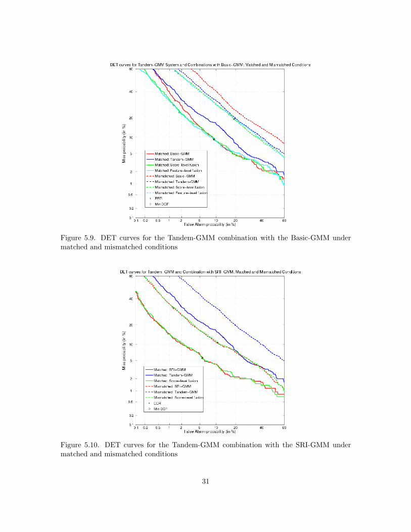
mismatched again refer to whether or not there are differences between the genders or handsets ofthe training and test data. Also, DET curves for these conditions are given in Figures 5.9 and 5.10for the Tandem-GMM combinations with the Basic-GMM and SRI-GMM, respectively. Similarto the Tandem/HATS-GMM system, the Tandem-GMM system performs better than the Basic-GMM for the mismatched condition, but worse for the matched condition. Over the entire DETcurve, the combinations with the Tandem-GMM yield consistent, significant improvement over theBasic-GMM for the mismatched case, but the gains are smaller and not always there in the matchedcondition. For the combination of the Tandem-GMM with the SRI-GMM, there is little change inthe DET curves from the baseline in either the matched or mismatched case, although the EERdoes improve in the matched condition.
5.3.3 HATS-GMM
The HATS-GMM system setup is shown in Figure 5.11. Only the HATS-MLP is used, but aswith the Tandem/HATS features, dimensionality reduction is applied, and the resulting featuresare input to a GMM speaker recognition system.
The minimum DCF and EER results for SRE2004 are given in Table 5.1 for the Basic-GMMsystem, the HATS-GMM system, and their score- and feature-level combinations. Also includedare results for the SRI-GMM system and its combination with the HATS-GMM. As before, changesrelative to each baseline (where a positive value indicates improvement) are shown in parentheses.
By itself, the HATS-GMM system is worse than the Basic-GMM system. Feature-level com-bination of MFCC and HATS features in a GMM system, as well as score-level combination of
29
Figure 5.7. DET curves for Tandem-GMM combination with Basic-GMM
Figure 5.8. DET curves for Tandem-GMM combination with SRI-GMM
30
Figure 5.9. DET curves for the Tandem-GMM combination with the Basic-GMM undermatched and mismatched conditions
Figure 5.10. DET curves for the Tandem-GMM combination with the SRI-GMM undermatched and mismatched conditions
Table 5.4. Fusion results with the Tandem-GMM system show improvements for the Basic-GMM, especially for the mismatched case, but only improvements in the matched conditionfor the SRI-GMM.
HATSNet
Speech Log GMMSystem
KLT51 framesof critical
band energy
HATS Features
Figure 5.11. HATS-GMM System Setup
the HATS-GMM system with the Basic-GMM do yield significant improvements, although not asgreat as for the Tandem/HATS-GMM and Tandem-GMM systems. These results are illustratedin Figure 5.12, which shows the DET curves of each system alone, along with the combinations.The HATS-GMM DET curve is noticeably worse than the Basic-GMM curve. In this case, thefeature-level fusion consistently yields better performance than the score-level combination, prob-ably because the HATS-GMM system alone performs so poorly. The gap between the Basic-GMMand the combinations with the HATS-GMM is smaller than it was for the Tandem/HATS-GMMand Tandem-GMM.
Table 5.5. HATS-GMM system results show gains for combination with the Basic-GMM,but none for fusion with the SRI-GMM.
As would be expected based on the previous Tandem/HATS-GMM and Tandem-GMM results,there is no improvement over the SRI-GMM baseline when it is combined with the HATS-GMM
32
Figure 5.12. DET curves for HATS-GMM combination with Basic-GMM
Figure 5.13. DET curves for HATS-GMM combination with SRI-GMM
33
system at the score-level. Once again, the DET curves in Figure 5.13 show that there is very littleseparation between the DET curve corresponding to the SRI-GMM system and the curve for thescore-level fusion of the SRI-GMM with the HATS-GMM.
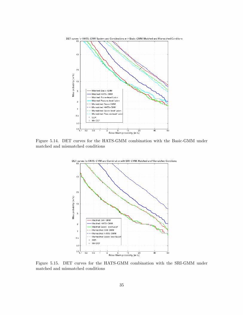
The results for both matched and mismatched conditions, which refer to whether or not thegenders and types of handsets of the training and test data are the same, are given in Table 5.6,and the DET curves are also separated into matched and mismatched conditions for the Basic-GMM and SRI-GMM combinations in Figures 5.14 and 5.15, respectively. The Basic-GMM systemis significantly better than the HATS-GMM system for the matched condition; however, the twosystems perform similarly for the mismatched condition, with each system performing better thanthe other over certain regions in the DET curve. For the matched condition, combination withthe HATS-GMM performs better than the Basic-GMM alone for high miss probabilities, but is notalways better for low miss probabilities. For the mismatched condition, however, the combinationsshow consistent improvement over the Basic-GMM baseline. For the SRI-GMM, combination withthe HATS-GMM yields very similar performance to the SRI-GMM alone, for both matched andmismatched conditions. The EER improves for the matched condition, although there is no changein EER for the mismatched case.
Table 5.6. Fusion results with the HATS-GMM system show improvements in the matchedand mismatched cases for the Basic-GMM, but only improvement in the matched case forthe SRI-GMM.
5.4 Results Using Speaker-MLP Features
5.4.1 Cross-validation Accuracies
The cross-validation results for the Speaker-MLPs are shown in Table 5.7 for each size MLP.It is clear that the CV accuracy increases with respect to the number of hidden units, for eachtraining speaker set. The accuracy increase on adding further hidden units does not appear tohave reached a plateau at 2500 hidden units for the 836 speaker net, though for the purposes ofthe current study the training times became prohibitive. With the computation shared between 4
34
Figure 5.14. DET curves for the HATS-GMM combination with the Basic-GMM undermatched and mismatched conditions
Figure 5.15. DET curves for the HATS-GMM combination with the SRI-GMM undermatched and mismatched conditions
35
CPUs, it took over 4 weeks to train the MLP with 2500 hidden units.
Number of speakers Hidden units CV Accuracy64 400 37.8%64 1000 47.8%128 1000 39.4%128 2000 44.5%836 400 20.5%836 800 25.5%836 1500 32.0%836 2500 35.5%
Table 5.7. CV accuracy improves as the number of hidden units increase.
5.4.2 Hidden Activations in SVM System (Speaker-SVM)
The basic setup for using the hidden activations from a Speaker-MLP in an SVM system isshown in Figure 5.16. After extracting the PLPs from the speech, these features are input tothe Speaker-MLP, and the hidden activations are converted into appropriate features (i.e., mean,standard deviation, histograms and percentiles along each dimension) for the SVM system.
Speech Log SVM featurecalculations
Speaker−MLP System
SVMSpeaker−MLP
21 framesof PLP
Hiddenactivations
Features
Figure 5.16. Speaker-SVM System Setup.
The SRE2004 results for the Speaker-SVMs are shown in Table 5.8 for each size MLP, whenusing the hidden activations as features in an SVM system. The speaker recognition results (bothDCF and EER) improve with an increase in the size of the hidden layer when considering a par-ticular number of training speakers.
The DET curves of the best Speaker-SVM systems for each set of training speakers are shownin Figure 5.17. Although the 64 speaker net performs the worst, there is only a small gap betweenits DET curve and the others. For the 128 and 836 speaker nets, there is really no advantage gainedby the larger (836 speaker) net, with very similar performance for the two.
In Table 5.9, the results are given for the score-level combination of the 64 speaker, 1000 hiddenunit, Speaker-SVM system with the Basic-GMM and SRI-GMM systems. For the SRI-GMM, thebest combination is yielded when the Speaker-MLP is trained with 64 speakers and 1000 hiddenunits (although the 128 speakers with 2000 hidden units does somewhat better in combination withthe Basic-GMM). There is a reasonable gain made when combining the Speaker-SVM system withthe Basic-GMM, but there is no significant improvement for the combination of the Speaker-SVM
Table 5.9. System combination with 64 speaker, 1000 hidden unit Speaker-SVM improvesBasic-GMM results, but not the SRI-GMM.
A further breakdown of the system combination results is given in Table 5.10. Here, matched(same gender and handset) and mismatched (different gender or handset) conditions between thetraining and test data are considered. When the Basic-GMM system is combined with the Speaker-SVM system, gains are made in both matched and mismatched conditions. For the state-of-the-artSRI-GMM baseline, combination with the Speaker-SVM system has marginal impact in either case.
Table 5.10. Fusion results with the Speaker-SVM system for both matched and mismatchedconditions show improvement for the Basic-GMM, but virtually no change for the SRI-GMM.
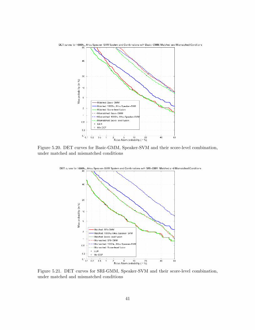
Examination of the DET curves for the matched and mismatched conditions reveals further in-sight into relative system performance. For the Basic-GMM and its combination with the Speaker-SVM system, the DET curves are shown in Figure 5.20. For the matched condition, the Speaker-SVM system outperforms the Basic-GMM for only a small range of high miss probabilities. Thescore-level combination of the two systems is better than the Basic-GMM over most of the curve,but the difference in performance lessens for higher false alarm probabilities. For the mismatchedcondition, the Speaker-SVM system outperforms the Basic-GMM over a larger range of probabili-ties. Furthermore, the combination of the two systems always outperforms the individual systems,with a more consistent gain over the entire range of miss and false alarm probabilities.
For the SRI-GMM system and its combination with the Speaker-SVM, the DET curves shownin Figure 5.21 tell a different story. For this score-level combination, there is virtually no improve-
38
Figure 5.18. DET curves for Speaker-SVM combination with Basic-GMM
Figure 5.19. DET curves for Speaker-SVM combination with SRI-GMM
39
ment over the SRI-GMM baseline, for either the matched or mismatched condition. Over the entirerange of miss and false alarm probabilities, the combination appears to be minutely worse than theSRI-GMM alone for the matched condition, and minutely better for the mismatched condition, butthere is no significant change in either case.
40
Figure 5.20. DET curves for Basic-GMM, Speaker-SVM and their score-level combination,under matched and mismatched conditions
Figure 5.21. DET curves for SRI-GMM, Speaker-SVM and their score-level combination,under matched and mismatched conditions
41
Chapter 6
Conclusion
Phonetic Tandem/HATS-MLP features were tested in a speaker recognition application. Al-though developed for ASR, the Tandem/HATS-MLP features still yield good results for a speakerrecognition task, and in fact perform better than a basic cepstral GMM system; even more im-provement comes from score- and feature-level combinations of the two, as shown in the summaryof results given in Table 6.1. Most of the improvement in performance is due to the Tandem-MLP component, which utilizes medium-term phonetic information (around 200 ms): standalone,the Tandem-GMM system yields even better results than the Tandem/HATS-GMM. When com-bined on the feature-level with MFCCs, however, the Tandem/HATS-MLP features yield slightlybetter results than the Tandem-MLP features, suggesting that the HATS-MLP component alsocontributes. The HATS-GMM system, which depends on long-term information (around 500ms),has the worst performance of the three phonetic MLP-based systems, although it still improvesupon the Basic-GMM in combination. A cepstral GMM system considers features computed forjust one frame at a time (typically 25 ms), so it is reasonable that the addition of features contain-ing longer-term information yields improvement over a basic cepstral GMM system alone. Theseimprovements do not translate to a state-of-the-art cepstral GMM system, however, as indicatedby the summary of results for fusion with the SRI-GMM given in Table 6.2.
Prior related work of both Heck and Konig, et al. and Wu and Morris, et al. has used dis-criminative features from MLPs trained to distinguish between speakers. Motivated by having awell-established infrastructure for neural network training at ICSI, my work tests a different, largerMLP topology of 3 layers, rather than 5, which I hoped would yield improved results. AlthoughWu and Morris, et al. have also tested 3-layer MLPs, there was a potential for making greater gainsby using more speakers, more hidden units, and a larger contextual window of cepstral features atthe input. Indeed, preliminary experiments indicated that using more training speakers would re-sult in a system that yields better results. Ultimately, however, a smaller subset of speakers chosenthrough clustering proved to be better. With fewer training speakers, the Speaker-MLP needs fewerparameters and can be trained in less time, yielding results comparable to those obtained using aSpeaker-MLP trained with a larger number of speakers, especially when considered in combinationwith a cepstral GMM system.
42
In comparison to the phonetic MLP features, the Speaker-MLP features yield results that aresimilar, although not quite as good. Even the best Speaker-SVM system does not perform as well asthe Tandem-GMM or Tandem/HATS-GMM systems. Furthermore, for a score-level combinationwith the Basic-GMM system, the Speaker-SVM system yields less improvement over the baselinethan the Tandem/HATS-GMM does (see Table 6.1). When considering a system fusion with theSRI-GMM, however, there is no significant difference between the performance of any of the MLP-based systems (see Table 6.2).
System Alone Feature-level Fusion Fusion with Basic-GMMDCF×10 EER (%) DCF×10 EER (%) DCF×10 EER (%)
Table 6.2. Results for the MLP-based systems and their score-level combinations with theSRI-GMM.
Although the MLP-based systems do not improve upon the SRI-GMM baseline in combination,this result could be explained by considering the difference in the performance between the two typesof systems: standalone, every MLP-based system performs much more poorly than the SRI-GMMdoes. The addition of channel compensating normalizations, such as T-norm, to an MLP-basedsystem should help reduce the performance gap between the MLP-based system and the SRI-GMM.It may then be possible for the MLP-based system to improve upon the state-of-the-art cepstralGMM system in combination, in the event that the performance gap is narrowed sufficiently.
Similar to results observed in prior work, the Speaker-SVM system improved speaker recognitionperformance for a basic cepstral GMM system; such a result was also true for the Tandem/HATS-GMM and other phonetic MLP-based systems. In the experiments of Wu and Morris, et al., gainswere observed when their MLP features system was combined with a basic GMM system, whichhad 32 Gaussians, and did not include CMS or channel and speaker normalizations. In the work ofHeck and Konig, et al., a state-of-the-art system including 1024 Gaussians, CMS, and H-norm wasused; at the time, however, channel compensation methods like channel mapping and speaker model
43
synthesis (SMS) were not invented and hence were not included in their cepstral GMM system.In comparison, the SRI-GMM is significantly improved by the addition of feature mapping, T-norm, as well as doubling the number of Gaussians to 2048. Heck and Konig, et al., observedthat for mismatched handsets, there was a consistent gain when combining the cepstral GMMwith their MLP features system. As evidenced by the results shown in Table 6.3, combinationsof the Basic-GMM with the phonetic- and speaker-discriminant MLP-based systems of this reportdo yield improvements, particularly for the mismatched condition (which refers to the trainingdata and test data being different genders or different handset types). However, Table 6.4 showsthe opposite result for combinations of the MLP-based systems with the SRI-GMM; while thereis still some improvement for the matched condition, there is virtually no improvement for themismatched condition. Although the previous work of Heck and Konig, et al., completed priorto the year 2000, showed that the greatest strength of an MLP-based approach was for the casewhen there is a handset mismatch between the training and test data, the state-of-the-art has sinceadvanced significantly in normalization and channel compensation techniques. As a result, thecontributions of the MLP-based systems, without any normalizations applied, to a state-of-the-artcepstral GMM system are no longer significant for the mismatched condition.
System Alone Fusion with Basic-GMMMatched Mismatched Matched MismatchedEER (%) EER (%) EER (%) EER (%)