Page 1
1
Phosphorus cycling in the settlement lagoon of a
treatment wetland
Santiago Jose Clerici
Submitted in accordance with the requirements for the degree of
Doctor of Philosophy
The University of Leeds
School of Earth and Environment
August 2013
Page 2
2
The candidate confirms that the work submitted is his/her own and that
appropriate credit has been given where reference has been made to the
work of others.
This copy has been supplied on the understanding that it is copyright
material and that no quotation from the thesis may be published without
proper acknowledgement.
The right of Santiago Jose Clerici to be identified as Author of this work
has been asserted by him in accordance with the Copyright, Designs and
Patents Act 1988.
© 2013 The University of Leeds and Santiago Jose Clerici
Page 3
3
Acknowledgements
I thank my supervisors Mike Krom, Rob Mortimer and Sally Mackenzie for their
constant support. My thanks also go to Sam Allshorn, David Ashley, Rachel
Spraggs, Cat Mcilwraith and Teresa Roncal Herrero for their assistance and
advice during field and laboratory work.
Page 4
4
Abstract
The South Finger treatment wetland at Slimbridge, UK, was designed to treat
water that has been impacted by the faeces of a dense population of waterfowl.
The wetland system has been failing consistently in retaining phosphorus (P). It
has been suggested that the settlement lagoon of the wetland is the cause for its
failure regarding P, because the lagoon exports P in the summer months. The aim
of this project was to understand the importance of the settlement lagoon in the
overall budget of P, and to understand the mechanisms that result in such
behaviour. This was achieved by measuring the fluxes of P in and out of the
lagoon, as well as measuring the fluxes through the sediment water interface and
the consumption/release of P by water column process. Also, an exhaustive study
of the chemistry of the pore waters and of the different species of P in the
sediments was carried out.
The data showed that the role of the settlement lagoon in the loading of P of the
treatment wetland is minimal. The sediments of the settlement lagoon release
dissolved P in the early summer, but this flux is much smaller than the mass of P
that enters the lagoon at the same time. The failure of the treatment wetland is
not related to the settlement lagoon, which has been performing satisfactorily in
retaining suspended solids and particulate P, but to the inadequate retention time
of the reed beds. This in turn is related to the original design of the wetland
system.
The source of the P that is released in the early summer is the bird faeces that
accumulate at the bottom of the lagoon through the winter. The accumulated
faeces are consumed rapidly in the early summer when temperature increases and
oxidisers are present in the pore waters the right conditions are present, releasing
their P through the sediment water interface (SWI). This process commences in
the early spring, with the appearance of an algal bloom, accompanied by high
levels of dissolved oxygen and the deposition of fresh algae onto the lagoon
sediments. Biodegradable algae is consumed by aerobic respiration above the
SWI at this time. The faeces, buried within the anaerobic sediments, are not
consumed significantly at this time however, because temperatures are still too
Page 5
5
low. The bacterial activity within the sediments, during the early summer, is
carried out mainly through iron and sulphate reduction.
At some time between March and June, temperatures increased and the
degradation of freshly deposited algae accelerates. This releases large quantities
of ammonium above the SWI, which triggers the combined process of
nitrification-denitrification, with nitrate reaching deep into the sediments. The
supply of nitrate into the sediments, accompanied by the increased temperatures,
accelerates the consumption of the buried bird faeces and the release of their
associated P through the SWI. By June, dissolved P is still released through the
SWI, although the consumption of the labile fraction of the bird faeces slows
down the rate of release. A small fraction of the released P is precipitated as
apatite within the sediments, without reaching the water column.
Page 6
6
Table of contents
ACKNOWLEDGEMENTS ........................................................................3
ABSTRACT ..............................................................................................4
TABLE OF CONTENTS ...........................................................................6
LIST OF FIGURES .................................................................................10
LIST OF TABLES...................................................................................17
1 INTRODUCTION .............................................................................19
1.1 Treatment wetlands.......................................................................................................19
1.1.1 Historical development...............................................................................................19
1.1.2 Free water surface constructed wetlands ....................................................................20
1.1.3 The retention of phosphorus by FWS constructed wetlands ......................................24
1.2 The Slimbridge Wetlands Centre ................................................................................25
1.2.1 Site history and description ........................................................................................25
1.2.2 The South Finger Treatment Wetland ........................................................................28
1.2.2.1 Construction of the South Finger treatment wetland ........................................28
1.2.2.2 Layout and operation of the South Finger treatment wetland ...........................29
1.2.3 Retention of P by the South Finger wetland ...............................................................32
1.2.3.1 The settlement lagoon as the source of excess P...............................................32
1.3 Aims of research, hypotheses and structure of the thesis ..........................................35
1.4 Relevance of the proposed study..................................................................................36
2 METHODS.......................................................................................41
2.1 Field methods.................................................................................................................41
2.1.1 Description of the pond ..............................................................................................41
2.1.2 Weather observations and weather data .....................................................................42
2.1.3 Bathymetric survey.....................................................................................................43
2.1.4 Water flow through the inlet.......................................................................................44
Page 7
7
2.1.5 Water sampling, frequency and replication................................................................46
2.1.5.1 Sampling the inlet .............................................................................................47
2.1.5.2 Sampling the pond ............................................................................................48
2.1.5.3 In situ water column incubations ......................................................................48
2.1.5.4 In situ benthic incubations ................................................................................50
2.1.6 Dissolved oxygen, pH and water temperature............................................................51
2.1.7 Sampling for chlorophyll ...........................................................................................52
2.1.8 Pore water chemistry..................................................................................................52
2.1.8.1 Diffusive Equilibrium in Thin (DET) gels .......................................................53
2.1.8.2 O2 probes ..........................................................................................................56
2.1.9 Sediment sampling .....................................................................................................56
2.2 Analytical methods .......................................................................................................60
2.2.1 Analysis of water samples..........................................................................................60
2.2.1.1 Speciation and analysis of phosphorus .............................................................60
2.2.1.2 Determination of ammonium and nitrate..........................................................61
2.2.1.3 Determination of chlorophyll ...........................................................................62
2.2.2 Analysis of DET gel sections .....................................................................................63
2.2.2.1 Determination of SRP.......................................................................................63
2.2.2.2 Determination of total dissolved iron ...............................................................64
2.2.2.3 Determination of ammonium, nitrate and sulphate...........................................65
2.2.2.4 Determination of calcium .................................................................................65
2.2.3 Analysis of sediment samples ....................................................................................65
2.2.3.1 Determination of porosity.................................................................................65
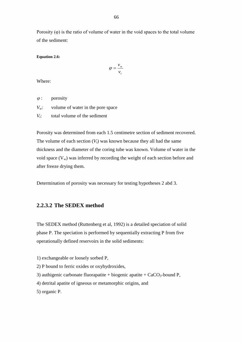
2.2.3.2 The SEDEX method .........................................................................................66
2.2.3.3 The Aspila method............................................................................................69
2.3 Sediment incubations....................................................................................................70
2.4 Calculations ...................................................................................................................71
2.4.1 Water balance.............................................................................................................71
2.4.2 Integration of the budgets of P ...................................................................................73
2.4.2.1 Mass balance of P in and out of the lagoon ......................................................73
2.4.2.2 Integration of the internal budgets of P ............................................................75
2.4.2.3 Fluxes of P through the SWI ............................................................................76
3.2.4.2 Fluxes of P within the water column ................................................................78
2.5 Release and retention of P from sediments.................................................................79
2.6 Methods summary ........................................................................................................80
3 LONG TERM WATER QUALITY DATA..........................................83
Page 8
8
3.1 Water quality prior to the construction of the South Finger wetland ......................83
3.2 Retention of P by the South Finger wetland ...............................................................88
3.3 General performance of the South Finger wetland....................................................93
4 BUDGETS OF PHOSPHORUS IN THE SETTLEMENT LAGOON.97
4.1 Introduction ...................................................................................................................97
4.2 Results ............................................................................................................................98
4.2.1 Weather observations .................................................................................................98
4.2.2 Bathymetry survey......................................................................................................99
4.2.3 Water balance ...........................................................................................................100
4.2.4 Phosphorus ...............................................................................................................102
4.2.4.1 SRP .................................................................................................................102
4.2.4.2 Dissolved organic P (DOP).............................................................................108
4.2.4.3 Particulate P (Part P).......................................................................................113
4.2.5 Biological activity indicators....................................................................................116
4.2.5.1 Chlorophyll .....................................................................................................116
4.2.5.2 Dissolved oxygen............................................................................................117
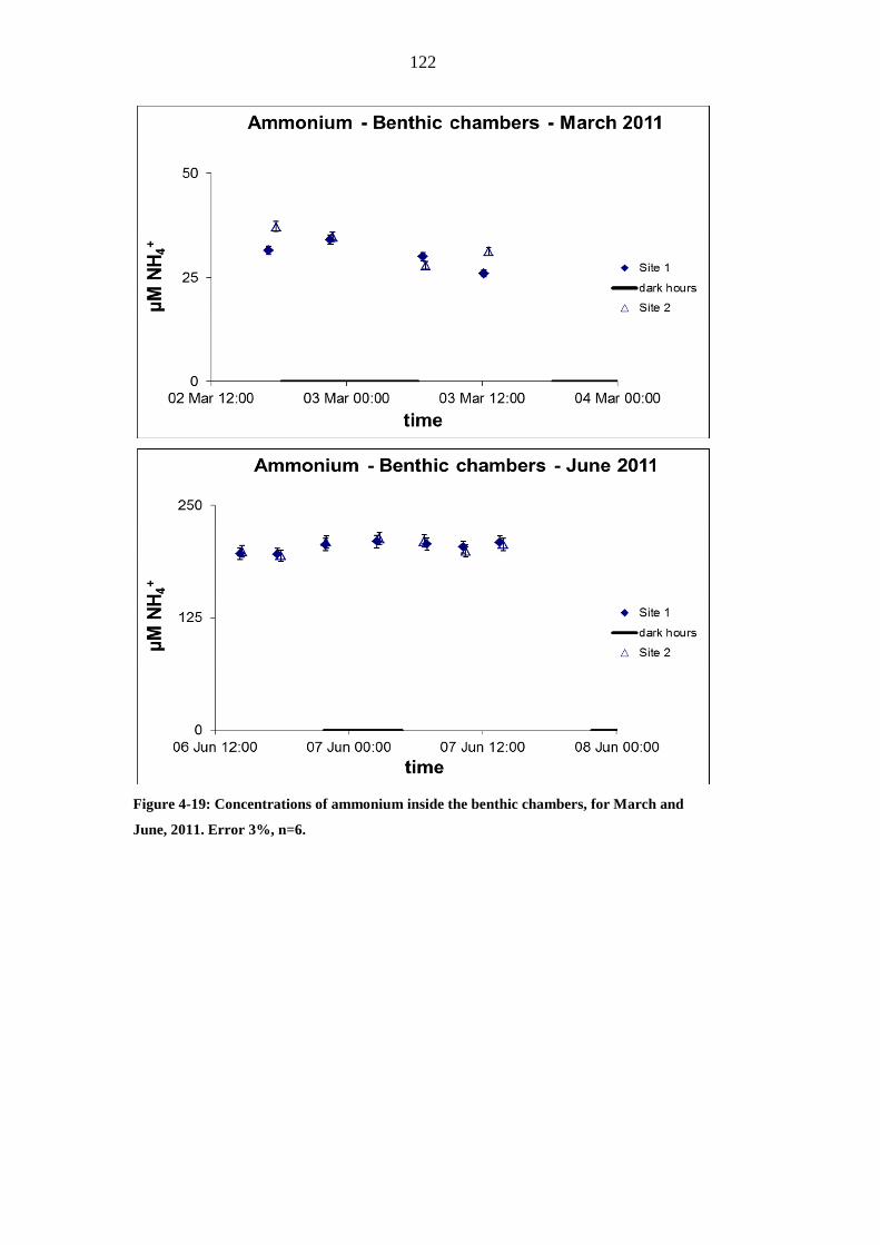
4.2.5.3 Ammonium .....................................................................................................120
4.3 Discussion.....................................................................................................................123
4.3.1 The budgets of P.......................................................................................................124
4.3.1.1 Spring..............................................................................................................124
4.3.1.2 Summer...........................................................................................................124
4.3.2 Cycling of P in spring...............................................................................................125
4.3.2.1 Settling of particulate P...................................................................................126
4.3.2.2 Mineralisation of Particulate P over the SWI..................................................126
4.3.3 Cycling of P in summer............................................................................................129
4.3.3.1 The dissolved species of P ..............................................................................129
4.3.3.2 Settling of particulate P...................................................................................130
4.3.3.3 Evidence of resuspension of Particulate P ......................................................131
5 BURIAL AND REGENERATION OF P IN THE SEDIMENTS OF
THE SETTLEMENT LAGOON .............................................................135
5.1 Introduction .................................................................................................................135
5.1.1 Relevance of sediments for the budgets of P in the settlement lagoon.....................135
5.1.2 Aim...........................................................................................................................135
Page 9
9
5.1.3 Background ..............................................................................................................136
5.1.3.1 Iron bound P ...................................................................................................137
5.1.3.2 Calcium bound P ............................................................................................138
5.1.3.3 Organic P ........................................................................................................139
5.2 Results ..........................................................................................................................141
5.2.1 Weather ....................................................................................................................141
5.2.2 Porosities..................................................................................................................142
5.2.3 Pore water DO..........................................................................................................143
5.2.4 Ammonium ..............................................................................................................145
5.2.5 Pore water nitrate .....................................................................................................148
5.2.6 Pore water sulphate ..................................................................................................150
5.2.7 Pore water iron .........................................................................................................153
5.2.8 Pore water calcium...................................................................................................156
5.2.9 Pore water SRP ........................................................................................................159
5.2.10 P speciation (SEDEX) .........................................................................................161
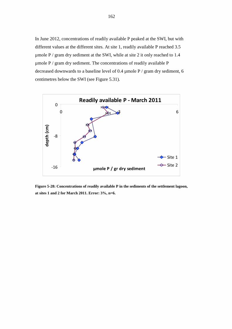
5.2.10.1 Readily available P .........................................................................................161
5.2.10.2 Iron bound P ...................................................................................................164
5.2.10.3 Apatite P .........................................................................................................166
5.2.10.4 Other inorganic P............................................................................................169
5.2.10.5 Organic P ........................................................................................................171
5.2.11 Pore water SRP from sediment incubations ........................................................174
5.3 Discussion ....................................................................................................................175
5.3.1 March 2011 ..............................................................................................................175
5.3.1.1 Water chemistry near the SWI........................................................................175
5.3.1.2 The solid phase ...............................................................................................176
5.3.2 June 2011 .................................................................................................................179
5.3.2.1 Water chemistry near the SWI........................................................................179
5.3.2.2 Chemistry of the pore water ...........................................................................180
5.3.2.3 The solid phase ...............................................................................................181
5.3.3 Mass balances and the controls for the release of P from sediments........................187
5.3.4 The sediments of the settlement lagoon in 2012, compared to 2011........................189
5.3.4.1 Organic P ........................................................................................................192
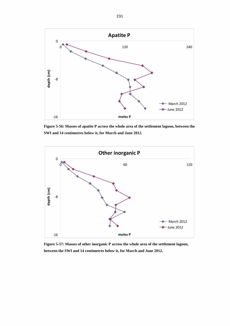
5.3.4.2 Apatite P .........................................................................................................193
6 SUMMARY ....................................................................................194
Spring .....................................................................................................................................195
Summer ..................................................................................................................................195
Page 10
10
7 CONCLUSIONS ............................................................................197
REFERENCES: ....................................................................................199
List of Figures
FIGURE 1-1: FOUR DIFFERENT TYPES OF CONSTRUCTED WETLANDS. A)
CONSTRUCTED WETLAND WITH FREE FLOATING PLANTS; B) FWS
CONSTRUCTED WETLAND; C) CONSTRUCTED WETLAND WITH HORIZONTAL
SUBSURFACE FLOW; AND D) CONSTRUCTED WETLAND WITH VERTICAL
SUBSURFACE FLOW (VIZAMAL 2007).........................................................................23
FIGURE 1-2: LAYOUT OF THE WWT SITE, SHOWING THE SOUTHFINGER WETLAND.
THE PONDS ARE INTERCONNECTED (NOT ALL CONNECTIONS SHOWN) AND
THEY DISCHARGE IN THE DITCH IMMEDIATELY UPSTREAM OF THE SOUTH
FINGER WETLAND. .........................................................................................................27
FIGURE 1-3: LAYOUT OF THE SOUTH FINGER TREATMENT WETLAND, AT THE
WILDFOWL AND WETLAND TRUST’S SITE IN SLIMBRIDGE.................................29
FIGURE 2-1: PLAN VIEW OF THE SETTLEMENT POND AT THE SOUTH FINGER
CONSTRUCTED WETLAND, WITH DETAIL OF POSITIONS OF INLETS, OUTLETS
AND SAMPLING POINTS 1 AND 2. ................................................................................42
FIGURE 2-2: DIPPING THE POND USING A FLAT BOTTOMED GRADUATED WOODEN
STAFF IN OCTOBER 2010. THE BOAT IS SECURED TO ONE OF THE
UNVEGETATED RAFTS. ON THE LEFT OF THE PHOTOGRAPH, ANOTHER RAFT
CAN BE SEEN WITH SOME VEGETATION ON IT.......................................................44
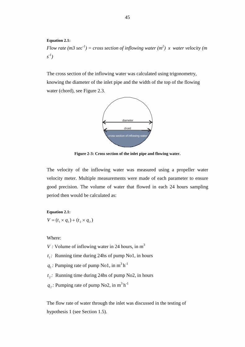
FIGURE 2-3: CROSS SECTION OF THE INLET PIPE AND FLOWING WATER..................45
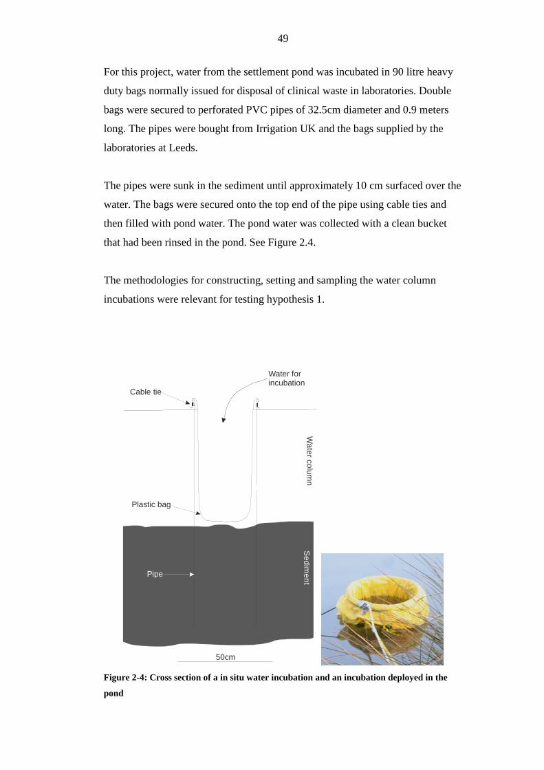
FIGURE 2-4: CROSS SECTION OF A IN SITU WATER INCUBATION AND AN
INCUBATION DEPLOYED IN THE POND.....................................................................49
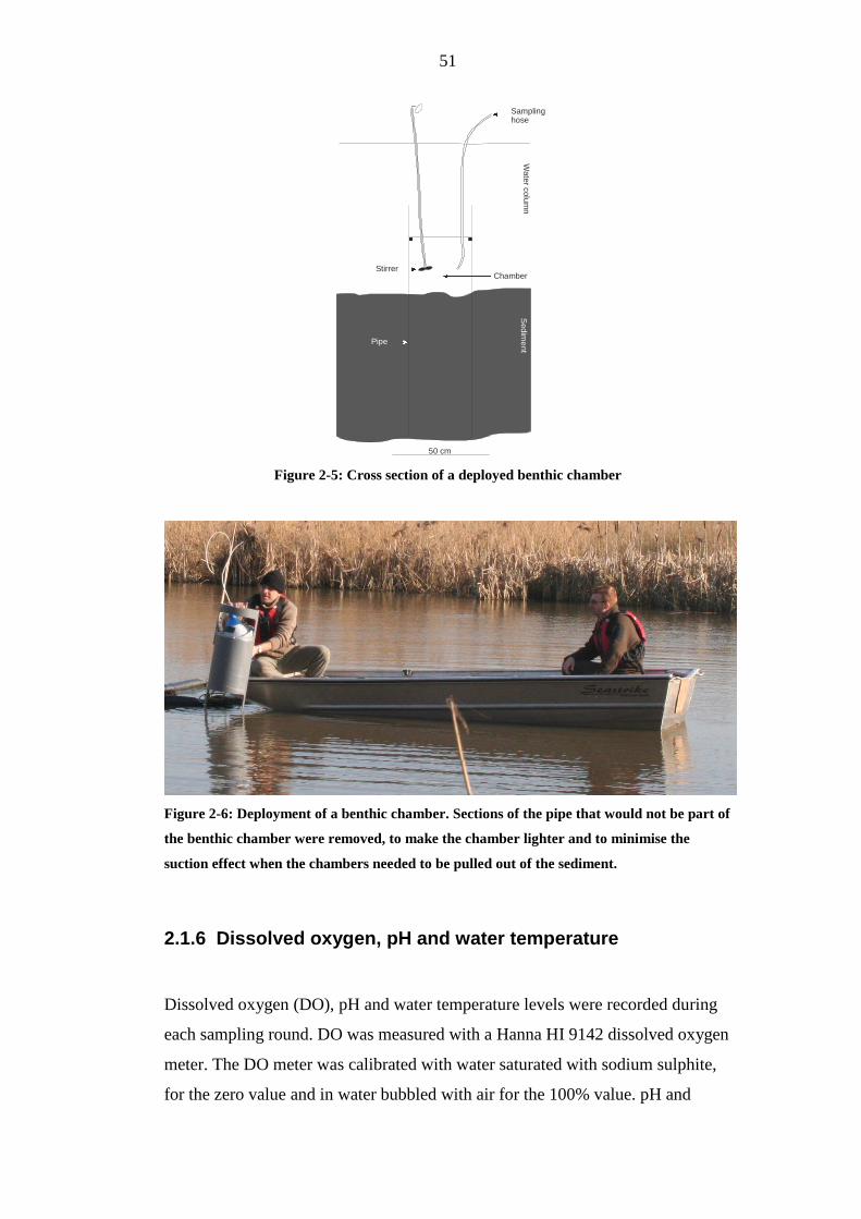
FIGURE 2-5: CROSS SECTION OF A DEPLOYED BENTHIC CHAMBER ...........................51
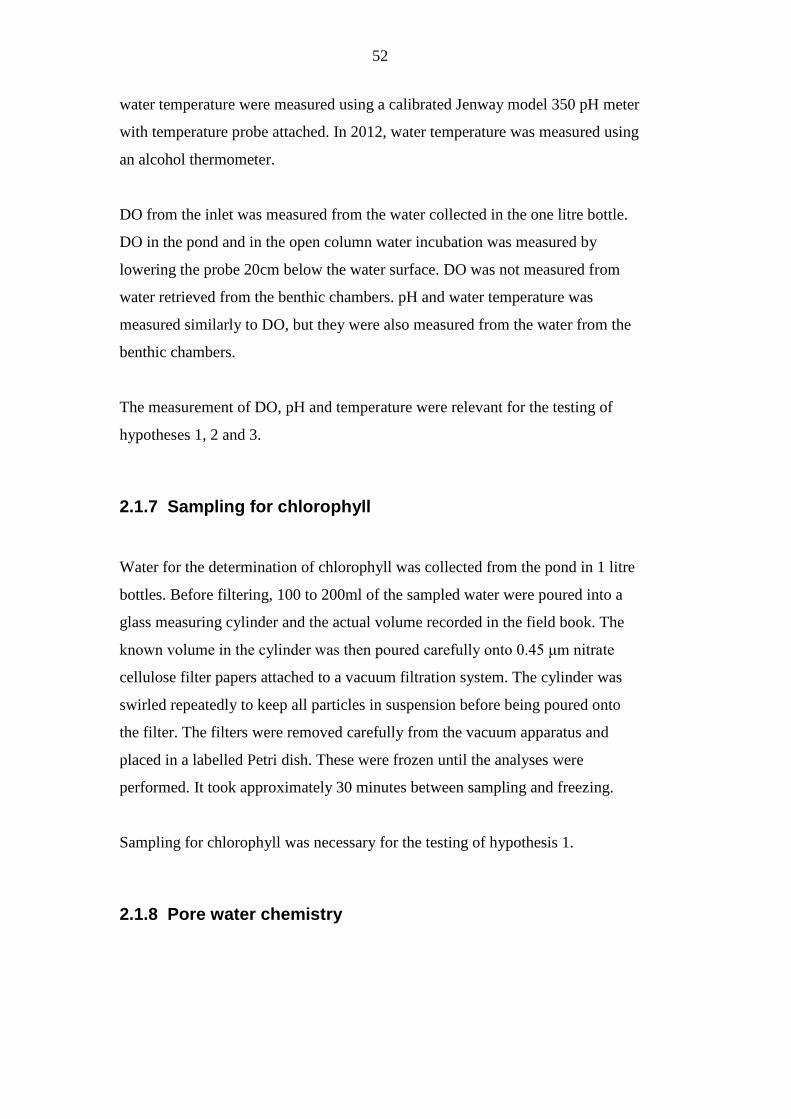
FIGURE 2-6: DEPLOYMENT OF A BENTHIC CHAMBER. SECTIONS OF THE PIPE THAT
WOULD NOT BE PART OF THE BENTHIC CHAMBER WERE REMOVED, TO
MAKE THE CHAMBER LIGHTER AND TO MINIMISE THE SUCTION EFFECT
WHEN THE CHAMBERS NEEDED TO BE PULLED OUT OF THE SEDIMENT........51
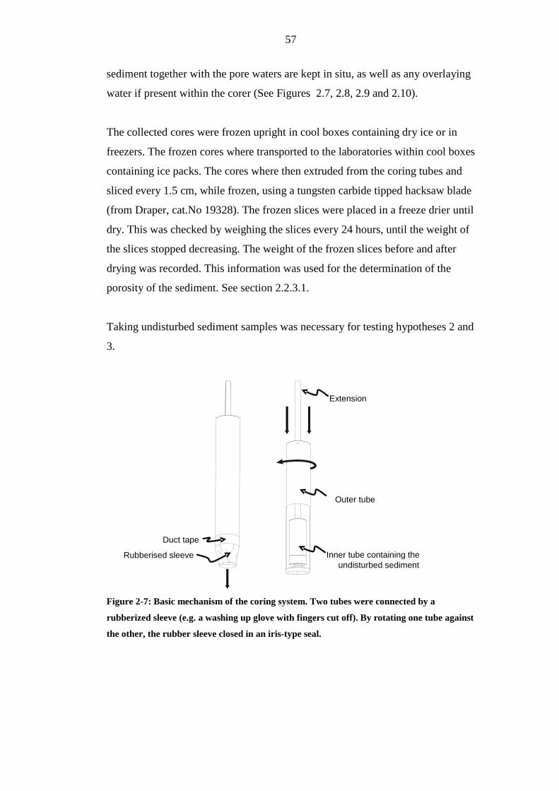
FIGURE 2-7: BASIC MECHANISM OF THE CORING SYSTEM. TWO TUBES WERE
CONNECTED BY A RUBBERIZED SLEEVE (E.G. A WASHING UP GLOVE WITH
FINGERS CUT OFF). BY ROTATING ONE TUBE AGAINST THE OTHER, THE
RUBBER SLEEVE CLOSED IN AN IRIS-TYPE SEAL...................................................57
FIGURE 2-8: CONSTRUCTION OF THE CORER. A) THE RUBBER SLEEVE WAS
ATTACHED TO THE INNER TUBE USING DUCT TAPE, AND AN EXTENSION
PIPE WAS SECURED BY THREADING A CABLE TIE THROUGH ALIGNED HOLES
Page 11
11
ON THE TUBES. B AND C) THE INNER TUBE AND EXTENSION WERE INSERTED
INTO THE OUTER TUBE AND THE RUBBER SLEEVE WAS THEN TURNED OVER
THE OUTER TUBE. D) THE RUBBER SLEEVE WAS SECURED TO THE OUTER
TUBE USING DUCT TAPE...............................................................................................58
FIGURE 2-9: RECOVERY OF THE UNDISTURBED CORES. A) THE RUBBERISED
SLEEVE WES SECURED ONTO THE INNER TUBE USING A CABLE TIE. B) THE
DUCT TAPE WAS PEELED OFF THE OUTER TUBE AND THEN C) THE OUTER
TUBE WAS SLID OFF KEEPING THE INNER TUBE ALWAYS VERTICAL. D) THE
EXTENSION HANDLE WES DISCONNECTED FROM THE INNER TUBE. THE
INNER TUBE CONTAINING THE SAMPLED CORE COULD THEN BE STORED,
AND A FRESH INNER TUBE INSERTED INTO THE CORING SYSTEM TO TAKE
THE FOLLOWING CORE. ................................................................................................59
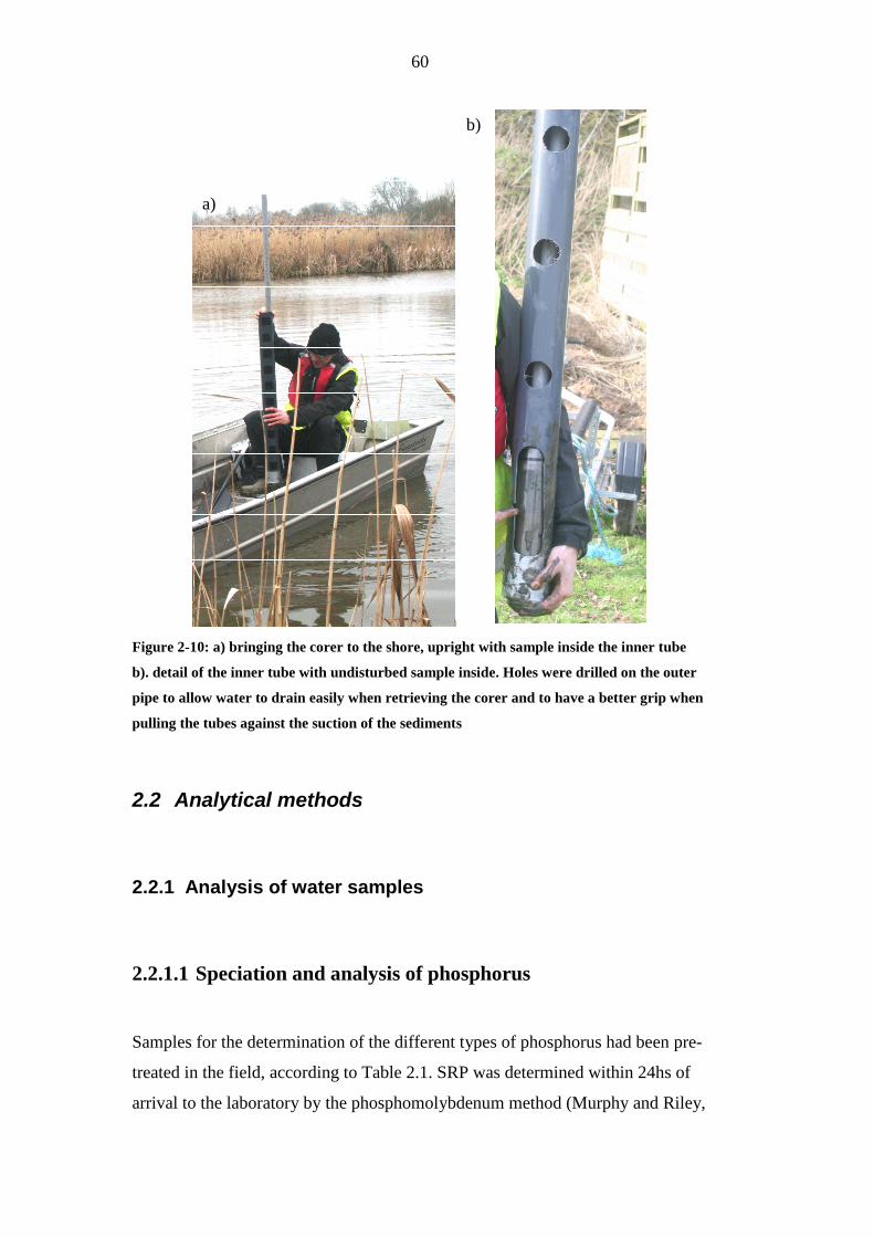
FIGURE 2-10: A) BRINGING THE CORER TO THE SHORE, UPRIGHT WITH SAMPLE
INSIDE THE INNER TUBE...............................................................................................60
FIGURE 2-11: THE FIVE PROGRESSIVE STEPS, USING DIFFERENT LEACHES OF
INCREASING STRENGTH, WHICH DISSOLVE INCREASINGLY INSOLUBLE
PHASES OF P IN THE PROCESS. ....................................................................................69
FIGURE 2-12: : SCHEMATIC REPRESENTATION OF THE DIFFERENT SOURCES AND
LOSES OF WATER CONSIDERED FOR THE CALCULATION OF THE WATER
BALANCE. THESE INCLUDE INFLOW (QIN), OUTFLOW (QOUT), INFILTRATION
(G), PRECIPITATION (P), EVAPORATION (E), AND THE DAILY CHANGES IN THE
VOLUME OF WATER (DV)..............................................................................................73
FIGURE 2-13: THE PROPOSED CYCLE OF P THAT WAS USED TO QUANTIFY THE
FLUXES OF P IN, OUT AND WITHIN THE SETTLEMENT LAGOON .......................76
FIGURE 3-1: LEVELS OF TSS IN WATER LEAVING THE VISITOR CENTRE PRIOR TO
THE CONSTRUCTION OF THE SOUTH FINGER WETLAND IN 1994, INFERRED
FROM 1995 AND 1996 DATA ..........................................................................................84
FIGURE 3-2: LEVELS OF BOD5, AMMONIA AND NITRATE IN WATER LEAVING THE
VISITOR CENTRE PRIOR TO THE CONSTRUCTION OF THE SOUTH FINGER
WETLAND IN 1994, INFERRED FROM 1995 AND 1996 DATA ..................................85
FIGURE 3-3: LEVELS OF ORTHOPHOSPHATE IN WATER LEAVING THE VISITOR
CENTRE PRIOR TO THE CONSTRUCTION OF THE SOUTH FINGER WETLAND IN
1994, INFERRED FROM 1995 AND 1996 DATA............................................................86
FIGURE 3-4: LEVELS OF ORTHOPHOSPHATE AT THE INLET AND OUTLET OF THE
SOUTH FINGER WETLAND, AS MONITORED AFTER COMMISSION IN 1995 AND
THEN SINCE 2005. ............................................................................................................89
FIGURE 3-5: LEVELS OF TSS AND BOD5 AT THE INLET AND OUTLET OF THE SOUTH
FINGER WETLAND, AS MONITORED AFTER COMMISSION IN 1995 AND THEN
SINCE 2005.........................................................................................................................94
Page 12
12
FIGURE 3-6: LEVELS OF AMMONIA AND NITRATE AT THE INLET AND OUTLET OF
THE SOUTH FINGER WETLAND, AS MONITORED AFTER COMMISSION IN 1995
AND THEN SINCE 2005....................................................................................................95
FIGURE 4-1: BATHYMETRIC SURVEY OF THE SETTLEMENT LAGOON. FIRST FIGURE
IS THE DEPTH TO THE BLACK UNCONSOLIDATED MATERIAL. SECOND
FIGURE IS THE DEPTH TO THE CLAY LINING. FIGURE BETWEEN BRACKETS IS
THE THICKNESS OF UNCONSOLIDATED MATERIAL............................................100
FIGURE 4-2: CONCENTRATIONS OF SRP THROUGH THE INLET, FOR MARCH AND
JUNE, 2011. ERROR 10%, N=6. ......................................................................................103
FIGURE 4-3: CONCENTRATIONS OF SRP IN THE WATER COLUMN, FOR MARCH
AND JUNE, 2011. ERROR 10%, N=6..............................................................................104
FIGURE 4.4: CONCENTRATIONS OF SRP INSIDE THE WATER COLUMN
INCUBATIONS, FOR MARCH AND JUNE, 2011. ERROR 10%, N=6. .......................105
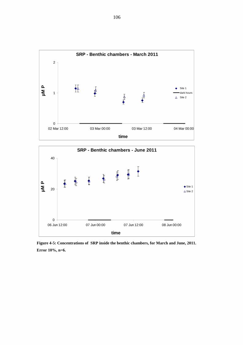
FIGURE 4-5: CONCENTRATIONS OF SRP INSIDE THE BENTHIC CHAMBERS, FOR
MARCH AND JUNE, 2011. ERROR 10%, N=6. .............................................................106
FIGURE 4-6: CONCENTRATIONS OF SRP AT THE BOTTOM OF THE WATER COLUMN
AND THROUGH THE SWI, SITES 1 AND 2 FOR MARCH AND JUNE, 2011...........107
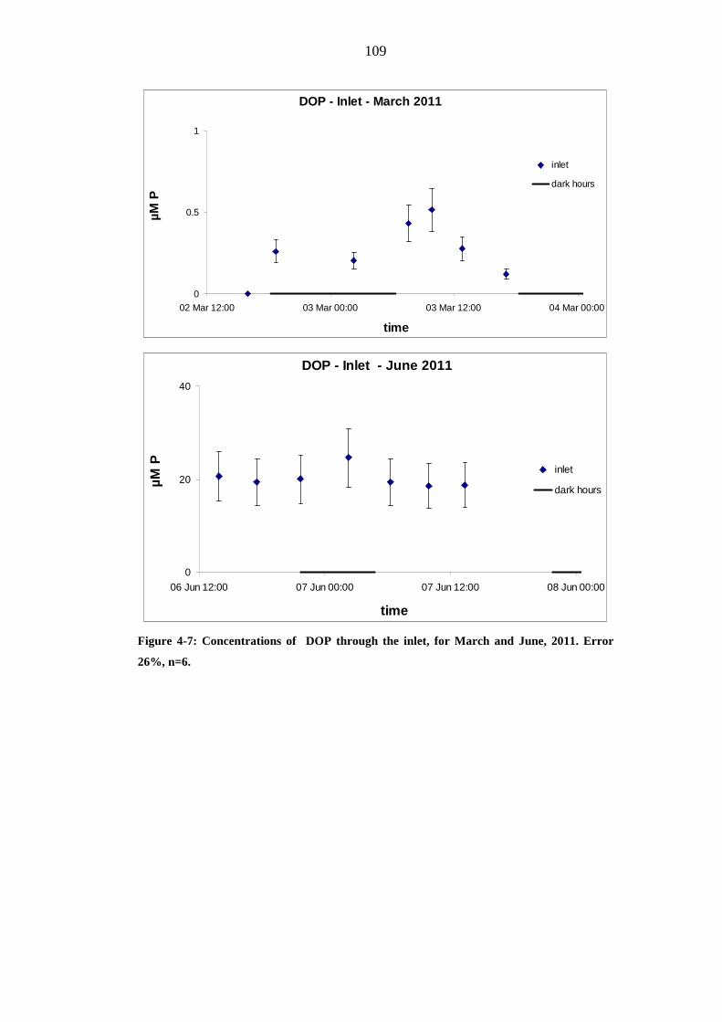
FIGURE 4-7: CONCENTRATIONS OF DOP THROUGH THE INLET, FOR MARCH AND
JUNE, 2011. ERROR 26%, N=6. ......................................................................................109
FIGURE 4-8: CONCENTRATIONS OF DOP IN THE WATER COLUMN, FOR MARCH
AND JUNE, 2011. ERROR 26%, N=6..............................................................................110
FIGURE 4.9: CONCENTRATIONS OF DOP INSIDE THE WATER COLUMN
INCUBATIONS, FOR MARCH AND JUNE, 2011. ERROR 26%, N=6. .......................111
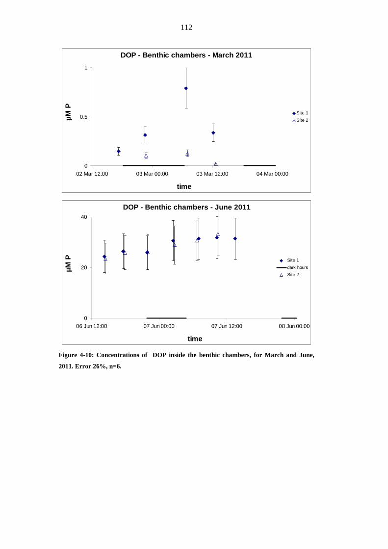
FIGURE 4-10: CONCENTRATIONS OF DOP INSIDE THE BENTHIC CHAMBERS, FOR
MARCH AND JUNE, 2011. ERROR 26%, N=6. .............................................................112
FIGURE 4-11: CONCENTRATIONS OF PART P THROUGH THE INLET, FOR MARCH
AND JUNE, 2011. ERROR 3%, N=6................................................................................114
FIGURE 4-12: CONCENTRATIONS OF PART P IN THE WATER COLUMN, FOR MARCH
AND JUNE, 2011. ERROR 3%, N=6................................................................................115
FIGURE 4-13: CONCENTRATIONS OF PART P INSIDE THE WATER COLUMN
INCUBATIONS, FOR MARCH AND JUNE, 2011. ERROR 3%, N=6. .........................116
FIGURE 4-14: : CONCENTRATIONS OF CHLOROPHYLL IN THE WATER COLUMN OF
THE SETTLEMENT LAGOON, EVERY TWO WEEKS, BETWEEN MARCH AND
JUNE 2011. ERROR: 15%, N=8 .......................................................................................117
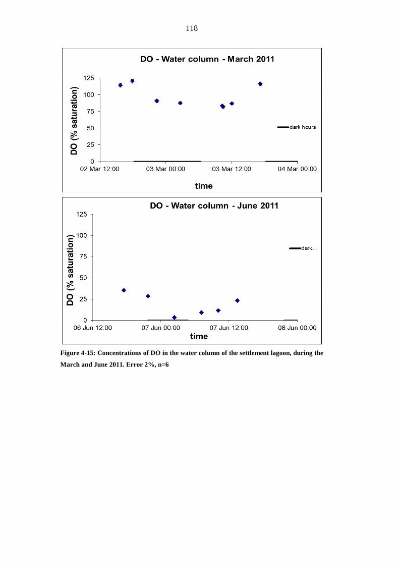
FIGURE 4-15: CONCENTRATIONS OF DO IN THE WATER COLUMN OF THE
SETTLEMENT LAGOON, DURING THE MARCH AND JUNE 2011. ERROR 2%, N=6
...........................................................................................................................................118
FIGURE 4-16: CONCENTRATIONS OF DO AT THE BOTTOM OF THE WATER COLUMN
AND THROUGH THE SWI, SITES 1 AND 2, DURING MARCH 2011. ......................119
Page 13
13
FIGURE 4-17: CONCENTRATIONS OF DO AT THE BOTTOM OF THE WATER COLUMN
AND THROUGH THE SWI, SITES 1 AND 2, DURING JUNE 2011............................120
FIGURE 4-18: CONCENTRATIONS OF AMMONIUM IN THE WATER COLUMN, FOR
MARCH AND JUNE, 2011. ERROR 3%, N=6................................................................121
FIGURE 4-19: CONCENTRATIONS OF AMMONIUM INSIDE THE BENTHIC CHAMBERS,
FOR MARCH AND JUNE, 2011. ERROR 3%, N=6. ......................................................122
FIGURE 4-20: CONCENTRATIONS OF AMMONIUM AT THE BOTTOM OF THE WATER
COLUMN AND THROUGH THE SWI, SITES 2 FOR MARCH, 2011, AND SITES 1
AND 2 FOR JUNE, 2011. .................................................................................................123
FIGURE 4-21: THE DAILY CYCLING OF P IN THE SETTLEMENT LAGOON, MARCH
2011 ...................................................................................................................................124
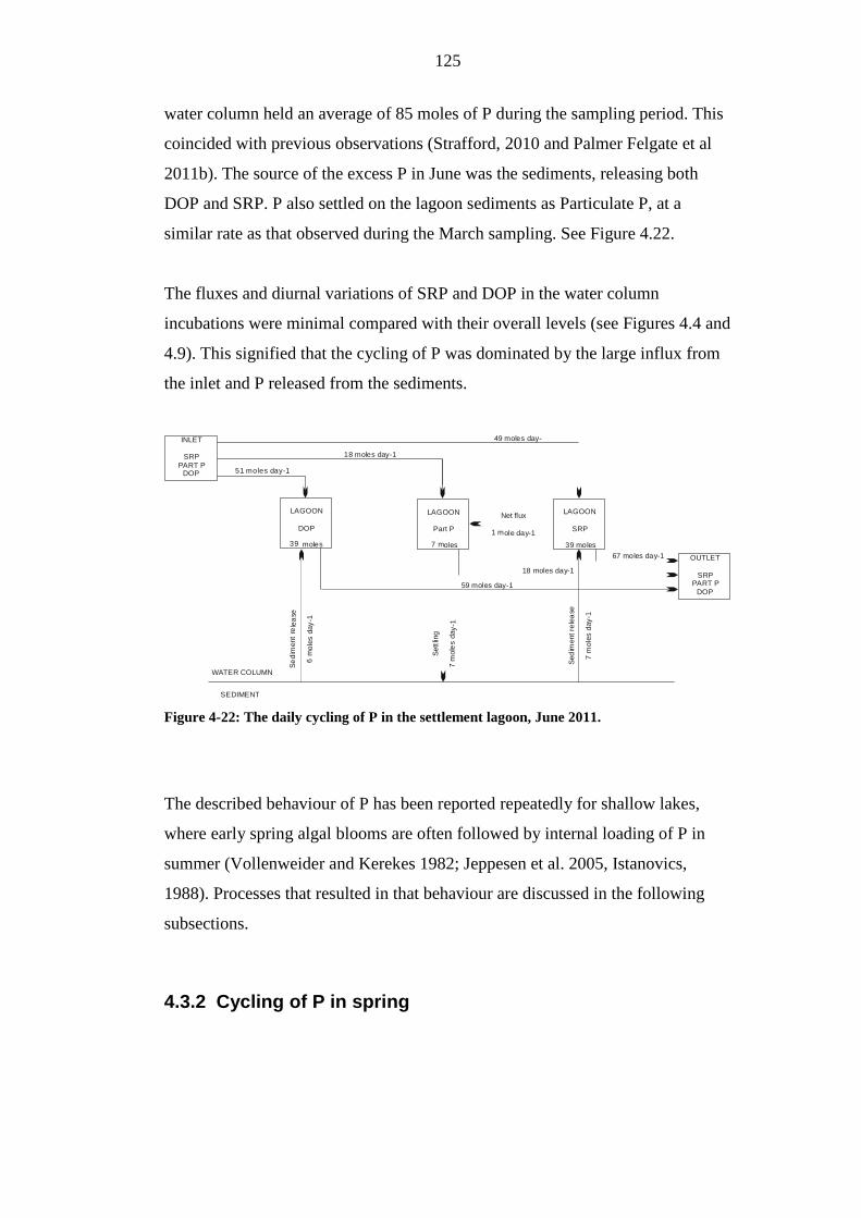
FIGURE 4-22: THE DAILY CYCLING OF P IN THE SETTLEMENT LAGOON, JUNE 2011.
...........................................................................................................................................125
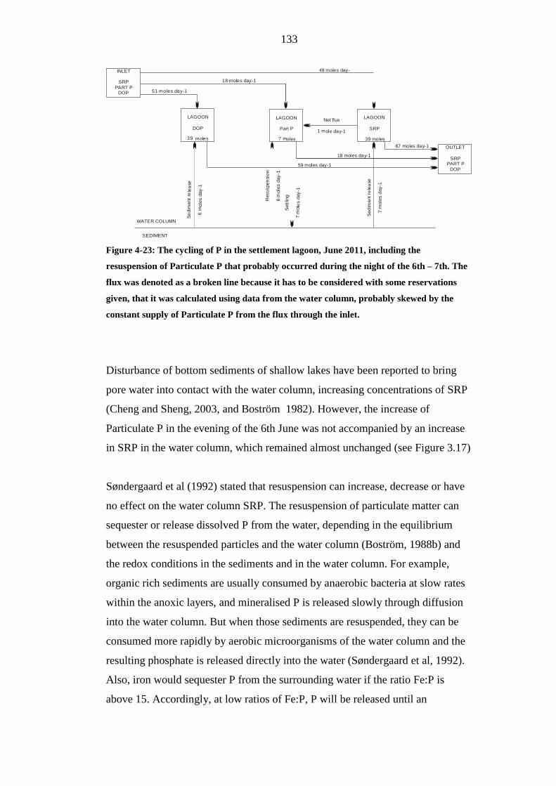
FIGURE 4-23: THE CYCLING OF P IN THE SETTLEMENT LAGOON, JUNE 2011,
INCLUDING THE RESUSPENSION OF PARTICULATE P THAT PROBABLY
OCCURRED DURING THE NIGHT OF THE 6TH – 7TH. THE FLUX WAS DENOTED
AS A BROKEN LINE BECAUSE IT HAS TO BE CONSIDERED WITH SOME
RESERVATIONS GIVEN, THAT IT WAS CALCULATED USING DATA FROM THE
WATER COLUMN, PROBABLY SKEWED BY THE CONSTANT SUPPLY OF
PARTICULATE P FROM THE FLUX THROUGH THE INLET...................................133
FIGURE 5-1: POROSITIES BETWEEN 0 AND 7 CENTIMETRES OF SEDIMENTS OF THE
SETTLEMENT LAGOON, MARCH AND JUNE, 2011 AND 2012. ERROR 2%, N=4 143
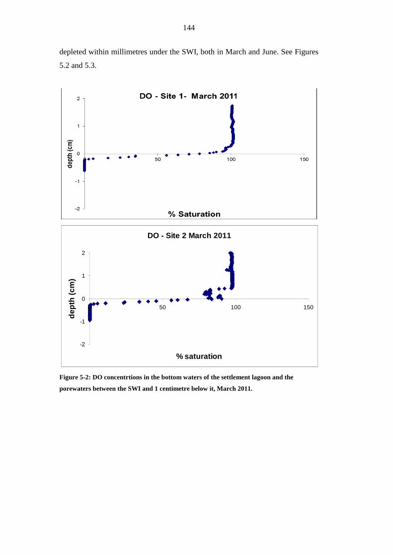
FIGURE 5-2: DO CONCENTRTIONS IN THE BOTTOM WATERS OF THE SETTLEMENT
LAGOON AND THE POREWATERS BETWEEN THE SWI AND 1 CENTIMETRE
BELOW IT, MARCH 2011...............................................................................................144
FIGURE 5-3: DO CONCENTRTIONS IN THE BOTTOM WATERS OF THE SETTLEMENT
LAGOON AND THE POREWATERS BETWEEN THE SWI AND 1 CENTIMETRE
BELOW IT, JUNE 2011....................................................................................................145
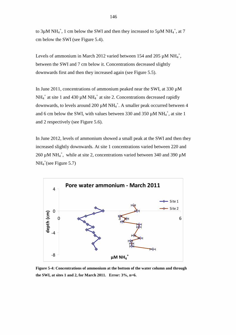
FIGURE 5-4: CONCENTRATIONS OF AMMONIUM AT THE BOTTOM OF THE WATER
COLUMN AND THROUGH THE SWI, AT SITES 1 AND 2, FOR MARCH 2011.
ERROR: 3%, N=6. ............................................................................................................146
FIGURE 5-5: CONCENTRATIONS OF AMMONIUM AT THE BOTTOM OF THE WATER
COLUMN AND THROUGH THE SWI, AT SITE 1 FOR MARCH 2012. ERROR: 3%,
N=6. ...................................................................................................................................147
FIGURE 5-6: CONCENTRATIONS OF AMMONIUM AT THE BOTTOM OF THE WATER
COLUMN AND THROUGH THE SWI, AT SITES 1 AND 2 FOR JUNE 2011. ERROR:
3%, N=6.............................................................................................................................147
FIGURE 5-7: CONCENTRATIONS OF AMMONIUM AT THE BOTTOM OF THE WATER
COLUMN AND THROUGH THE SWI, AT SITES 1 AND 2 FOR JUNE 2012. ERROR:
3%, N=6.............................................................................................................................148
Page 14
14
FIGURE 5-8: CONCENTRATIONS OF NITRATE AT THE BOTTOM OF THE WATER
COLUMN AND THROUGH THE SWI, AT SITE 2 FOR MARCH 2011. ERROR: 10%,
N=8. ...................................................................................................................................149
FIGURE 5-9: CONCENTRATIONS OF NITRATE AT THE BOTTOM OF THE WATER
COLUMN AND THROUGH THE SWI, AT SITES 1 AND 2 FOR MARCH 2012.
ERROR: 10%, N=8............................................................................................................149
FIGURE 5-10: CONCENTRATIONS OF NITRATE AT THE BOTTOM OF THE WATER
COLUMN AND THROUGH THE SWI, AT SITE 2 FOR JUNE 2011. ERROR: 10%, N=8.
...........................................................................................................................................150
FIGURE 5-11: CONCENTRATIONS OF NITRATE AT THE BOTTOM OF THE WATER
COLUMN AND THROUGH THE SWI, AT SITE 1 FOR JUNE 2012. ERROR: 10%, N=8.
...........................................................................................................................................150
FIGURE 5-12: CONCENTRATIONS OF SULPHATE AT THE BOTTOM OF THE WATER
COLUMN AND THROUGH THE SWI, AT SITE 2 FOR MARCH 2011. ERROR: 5%,
N=5. ...................................................................................................................................151
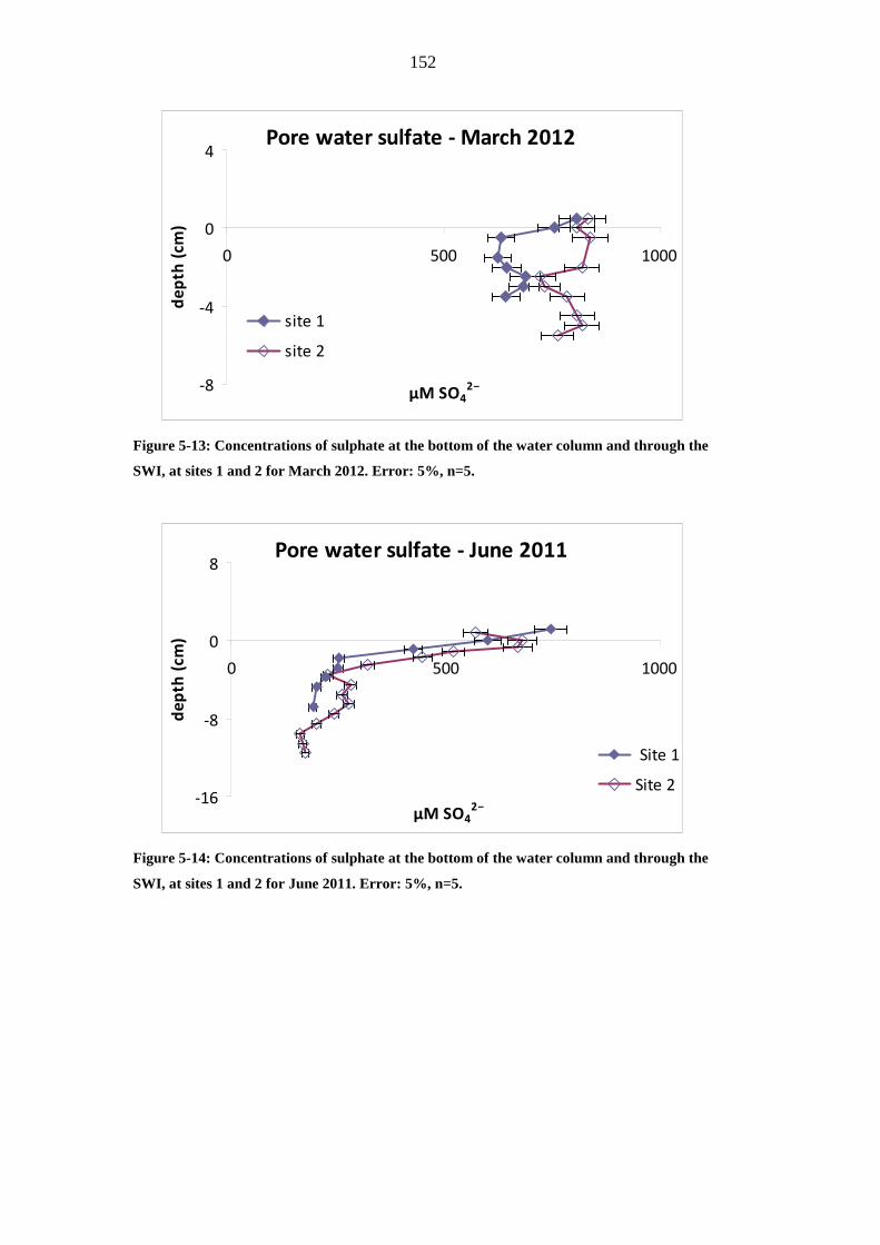
FIGURE 5-13: CONCENTRATIONS OF SULPHATE AT THE BOTTOM OF THE WATER
COLUMN AND THROUGH THE SWI, AT SITES 1 AND 2 FOR MARCH 2012.
ERROR: 5%, N=5..............................................................................................................152
FIGURE 5-14: CONCENTRATIONS OF SULPHATE AT THE BOTTOM OF THE WATER
COLUMN AND THROUGH THE SWI, AT SITES 1 AND 2 FOR JUNE 2011. ERROR:
5%, N=5. ............................................................................................................................152
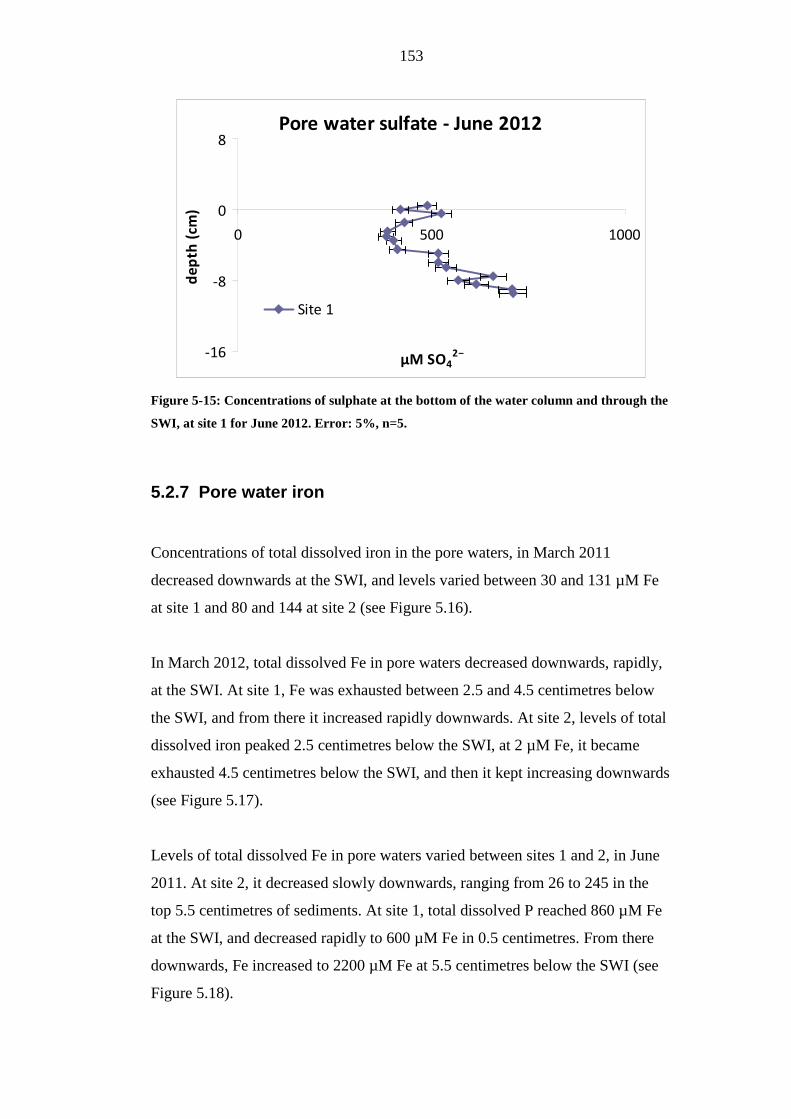
FIGURE 5-15: CONCENTRATIONS OF SULPHATE AT THE BOTTOM OF THE WATER
COLUMN AND THROUGH THE SWI, AT SITE 1 FOR JUNE 2012. ERROR: 5%, N=5.
...........................................................................................................................................153
FIGURE 5-16: CONCENTRATIONS OF IRON AT THE BOTTOM OF THE WATER
COLUMN AND THROUGH THE SWI, AT SITES 1 AND 2 FOR MARCH 2011.
ERROR: 8%, N=6..............................................................................................................154
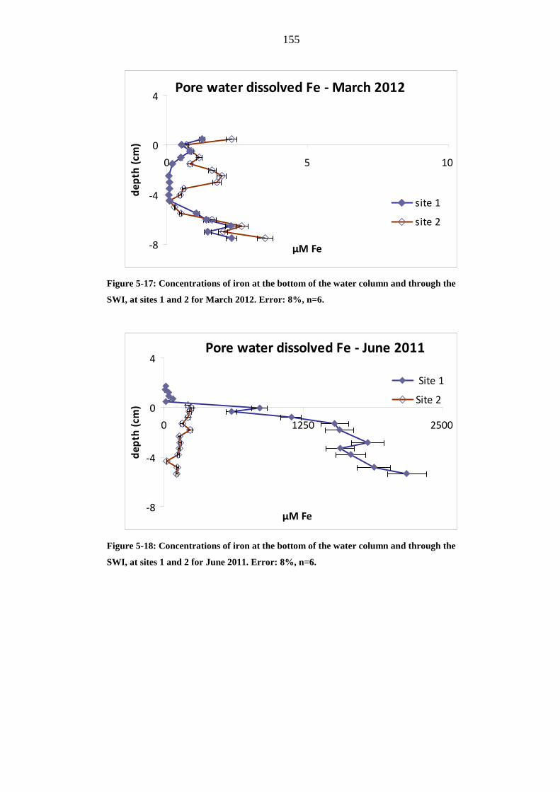
FIGURE 5-17: CONCENTRATIONS OF IRON AT THE BOTTOM OF THE WATER
COLUMN AND THROUGH THE SWI, AT SITES 1 AND 2 FOR MARCH 2012.
ERROR: 8%, N=6..............................................................................................................155
FIGURE 5-18: CONCENTRATIONS OF IRON AT THE BOTTOM OF THE WATER
COLUMN AND THROUGH THE SWI, AT SITES 1 AND 2 FOR JUNE 2011. ERROR:
8%, N=6. ............................................................................................................................155
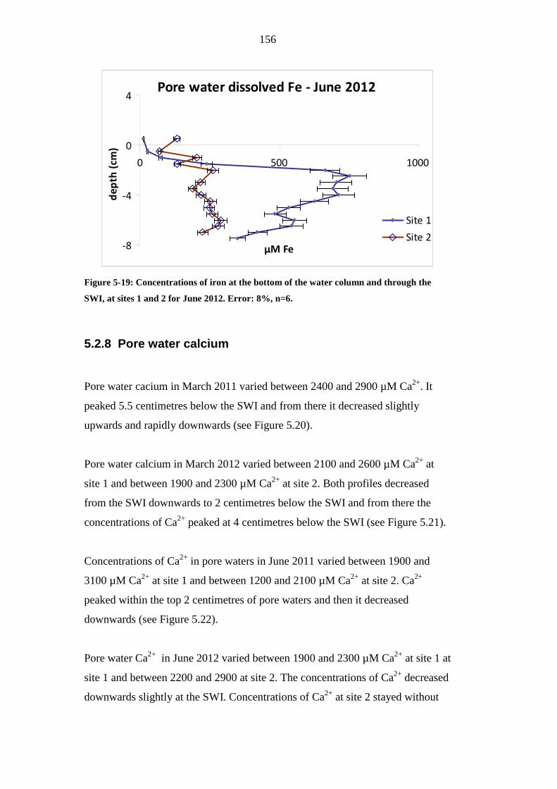
FIGURE 5-19: CONCENTRATIONS OF IRON AT THE BOTTOM OF THE WATER
COLUMN AND THROUGH THE SWI, AT SITES 1 AND 2 FOR JUNE 2012. ERROR:
8%, N=6. ............................................................................................................................156
FIGURE 5-20: CONCENTRATIONS OF CALCIUM AT THE BOTTOM OF THE WATER
COLUMN AND THROUGH THE SWI, AT SITE 2 FOR MARCH 2011. ERROR: 0%,
N=6. ...................................................................................................................................157
Page 15
15
FIGURE 5-21: CONCENTRATIONS OF CALCIUM AT THE BOTTOM OF THE WATER
COLUMN AND THROUGH THE SWI, AT SITES 1 AND 2 FOR MARCH 2012.
ERROR: 0%, N=6. ............................................................................................................157
FIGURE 5-22: CONCENTRATIONS OF CALCIUM AT THE BOTTOM OF THE WATER
COLUMN AND THROUGH THE SWI, AT SITES 1 AND 2 FOR JUNE 2011. ERROR:
0%, N=6.............................................................................................................................158
FIGURE 5-23: CONCENTRATIONS OF CALCIUM AT THE BOTTOM OF THE WATER
COLUMN AND THROUGH THE SWI, AT SITES 1 AND 2 FOR JUNE 2012. ERROR:
0%, N=6.............................................................................................................................158
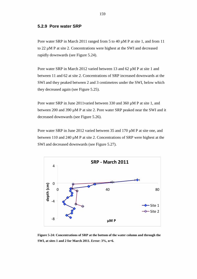
FIGURE 5-24: CONCENTRATIONS OF SRP AT THE BOTTOM OF THE WATER COLUMN
AND THROUGH THE SWI, AT SITES 1 AND 2 FOR MARCH 2011. ERROR: 3%, N=6.
...........................................................................................................................................159
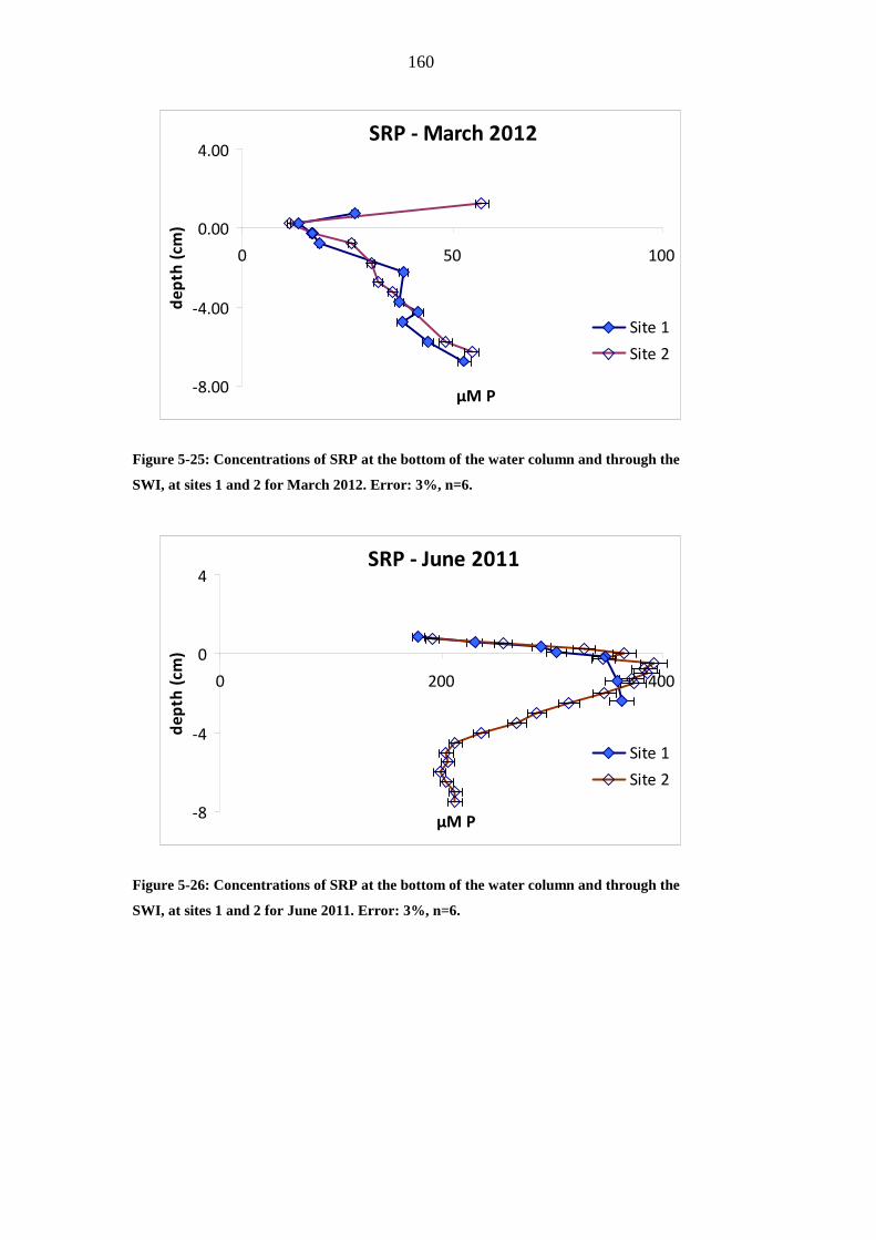
FIGURE 5-25: CONCENTRATIONS OF SRP AT THE BOTTOM OF THE WATER COLUMN
AND THROUGH THE SWI, AT SITES 1 AND 2 FOR MARCH 2012. ERROR: 3%, N=6.
...........................................................................................................................................160
FIGURE 5-26: CONCENTRATIONS OF SRP AT THE BOTTOM OF THE WATER COLUMN
AND THROUGH THE SWI, AT SITES 1 AND 2 FOR JUNE 2011. ERROR: 3%, N=6.
...........................................................................................................................................160
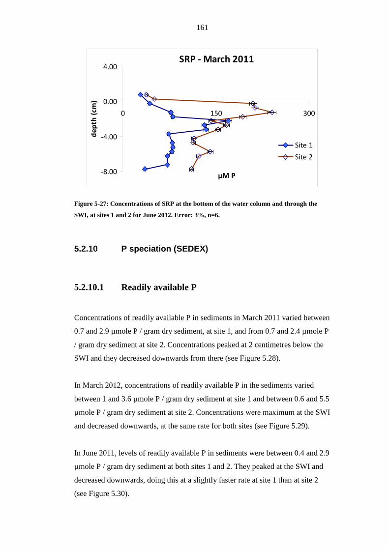
FIGURE 5-27: CONCENTRATIONS OF SRP AT THE BOTTOM OF THE WATER COLUMN
AND THROUGH THE SWI, AT SITES 1 AND 2 FOR JUNE 2012. ERROR: 3%, N=6.
...........................................................................................................................................161
FIGURE 5-28: CONCENTRATIONS OF READILY AVAILABLE P IN THE SEDIMENTS OF
THE SETTLEMENT LAGOON, AT SITES 1 AND 2 FOR MARCH 2011. ERROR: 3%,
N=6. ...................................................................................................................................162
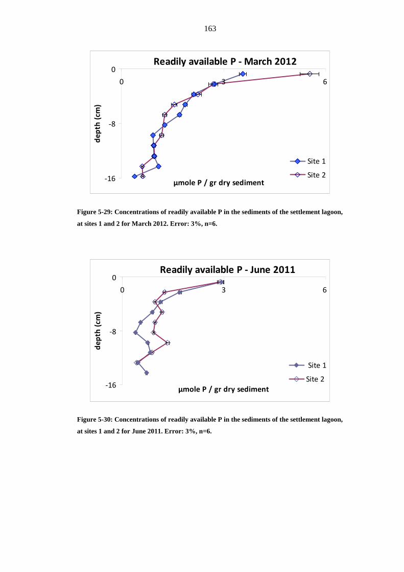
FIGURE 5-29: CONCENTRATIONS OF READILY AVAILABLE P IN THE SEDIMENTS OF
THE SETTLEMENT LAGOON, AT SITES 1 AND 2 FOR MARCH 2012. ERROR: 3%,
N=6. ...................................................................................................................................163
FIGURE 5-30: CONCENTRATIONS OF READILY AVAILABLE P IN THE SEDIMENTS OF
THE SETTLEMENT LAGOON, AT SITES 1 AND 2 FOR JUNE 2011. ERROR: 3%,
N=6. ...................................................................................................................................163
FIGURE 5-31: CONCENTRATIONS OF READILY AVAILABLE P IN THE SEDIMENTS OF
THE SETTLEMENT LAGOON, AT SITES 1 AND 2 FOR JUNE 2012. ERROR: 3%,
N=6. ...................................................................................................................................164
FIGURE 5-32: CONCENTRATIONS OF IRON BOUND P IN THE SEDIMENTS OF THE
SETTLEMENT LAGOON, AT SITES 1 AND 2 FOR MARCH 2011. ERROR: 24%, N=6.
...........................................................................................................................................165
FIGURE 5-33: CONCENTRATIONS OF IRON BOUND P IN THE SEDIMENTS OF THE
SETTLEMENT LAGOON, AT SITES 1 AND 2 FOR MARCH 2012. ERROR: 24%, N=6.
...........................................................................................................................................165
Page 16
16
FIGURE 5-34: CONCENTRATIONS OF IRON BOUND P IN THE SEDIMENTS OF THE
SETTLEMENT LAGOON, AT SITES 1 AND 2 FOR JUNE 2011. ERROR: 24%, N=6.
...........................................................................................................................................166
FIGURE 5-35: CONCENTRATIONS OF IRON BOUND P IN THE SEDIMENTS OF THE
SETTLEMENT LAGOON, AT SITES 1 AND 2 FOR JUNE 2012. ERROR: 24%, N=6.
...........................................................................................................................................166
FIGURE 5-36: CONCENTRATIONS OF APATITE P IN THE SEDIMENTS OF THE
SETTLEMENT LAGOON, AT SITES 1 AND 2 FOR MARCH 2011. ERROR: 7%, N=6.
...........................................................................................................................................167
FIGURE 5-37: CONCENTRATIONS OF APATITE P IN THE SEDIMENTS OF THE
SETTLEMENT LAGOON, AT SITES 1 AND 2 FOR MARCH 2012. ERROR: 7%, N=6.
...........................................................................................................................................168
FIGURE 5-38: CONCENTRATIONS OF APATITE P IN THE SEDIMENTS OF THE
SETTLEMENT LAGOON, AT SITES 1 AND 2 FOR JUNE 2011. ERROR: 7%, N=6..168
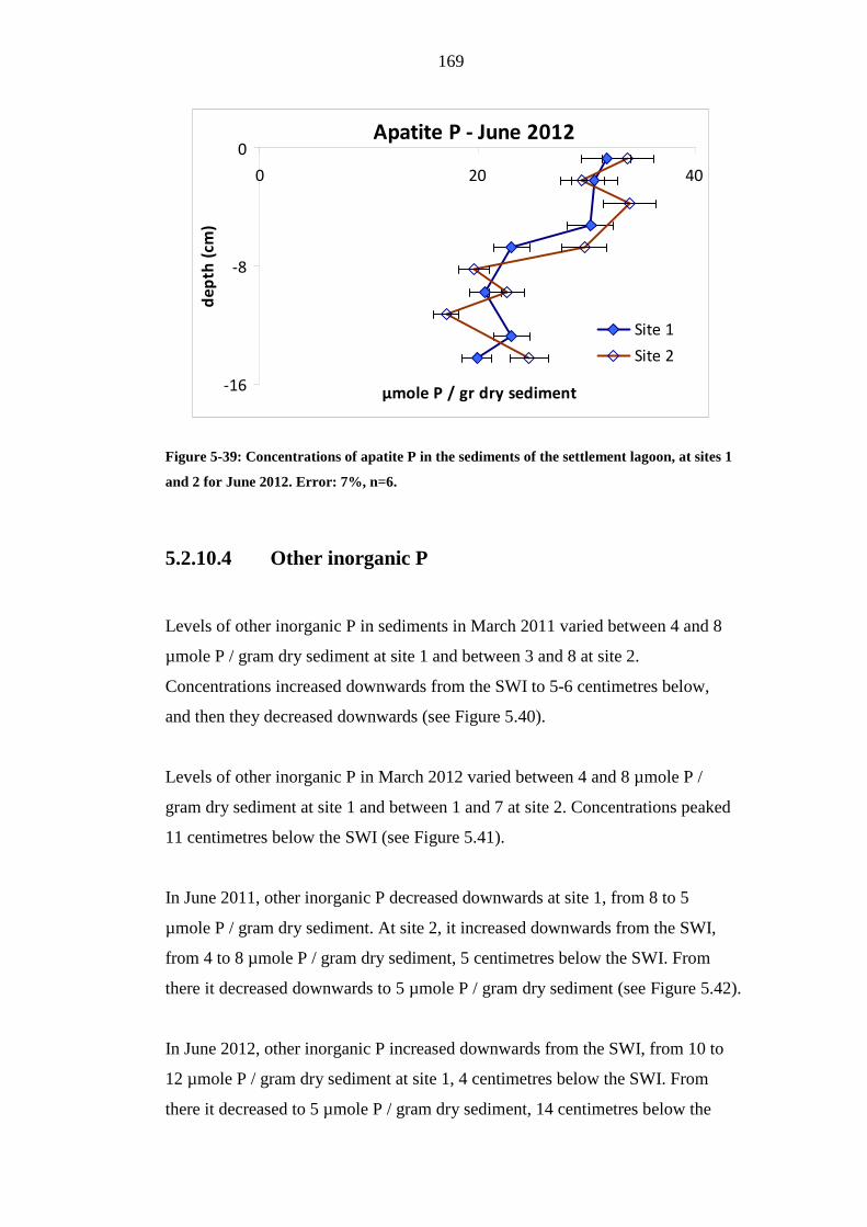
FIGURE 5-39: CONCENTRATIONS OF APATITE P IN THE SEDIMENTS OF THE
SETTLEMENT LAGOON, AT SITES 1 AND 2 FOR JUNE 2012. ERROR: 7%, N=6..169
FIGURE 5-40: CONCENTRATIONS OF OTHER INORGANIC P IN THE SEDIMENTS OF
THE SETTLEMENT LAGOON, AT SITES 1 AND 2 FOR MARCH 2011. ERROR: 13%,
N=6. ...................................................................................................................................170
FIGURE 5-41: CONCENTRATIONS OF OTHER INORGANIC P IN THE SEDIMENTS OF
THE SETTLEMENT LAGOON, AT SITES 1 AND 2 FOR MARCH 2012. ERROR: 13%,
N=6. ...................................................................................................................................170
FIGURE 5-42: CONCENTRATIONS OF OTHER INORGANIC P IN THE SEDIMENTS OF
THE SETTLEMENT LAGOON, AT SITES 1 AND 2 FOR JUNE 2011. ERROR: 13%,
N=6. ...................................................................................................................................171
FIGURE 5-43: CONCENTRATIONS OF OTHER INORGANIC P IN THE SEDIMENTS OF
THE SETTLEMENT LAGOON, AT SITES 1 AND 2 FOR JUNE 2012. ERROR: 13%,
N=6. ...................................................................................................................................171
FIGURE 5-44: CONCENTRATIONS OF OTHER ORGANIC P IN THE SEDIMENTS OF THE
SETTLEMENT LAGOON, AT SITES 1 AND 2 FOR MARCH 2011. ERROR: 10%, N=6.
...........................................................................................................................................172
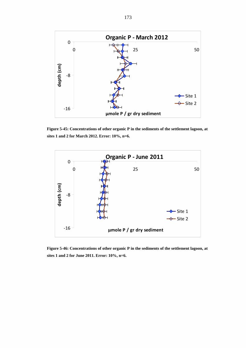
FIGURE 5-45: CONCENTRATIONS OF OTHER ORGANIC P IN THE SEDIMENTS OF THE
SETTLEMENT LAGOON, AT SITES 1 AND 2 FOR MARCH 2012. ERROR: 10%, N=6.
...........................................................................................................................................173
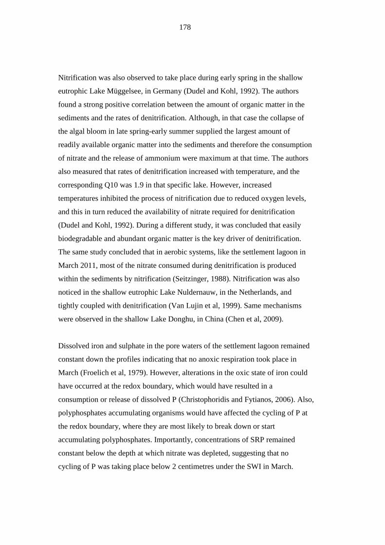
FIGURE 5-46: CONCENTRATIONS OF OTHER ORGANIC P IN THE SEDIMENTS OF THE
SETTLEMENT LAGOON, AT SITES 1 AND 2 FOR JUNE 2011. ERROR: 10%, N=6.
...........................................................................................................................................173
FIGURE 5-47: CONCENTRATIONS OF OTHER ORGANIC P IN THE SEDIMENTS OF THE
SETTLEMENT LAGOON, AT SITES 1 AND 2 FOR JUNE 2012. ERROR: 10%, N=6.
...........................................................................................................................................174
Page 17
17
FIGURE 5-48: CONCENTRATIONS OF SRP IN PORE WATER OF SEDIMENT
INCUBATIONS, BETWEEN TIME=0 AND TIME=5 DAYS. EACH SAMPLE WAS
INCUBATED, SAMPLED AND ANALYSED IN TRIPLICATE. THEREFORE, THE
ERROR BARS REPRESENT ONE STANDARD DEVIATION (N=3)..........................175
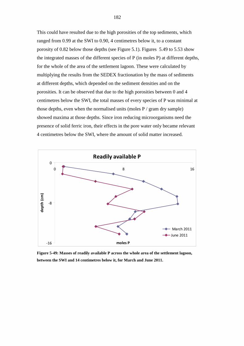
FIGURE 5-49: MASSES OF READILY AVAILABLE P ACROSS THE WHOLE AREA OF
THE SETTLEMENT LAGOON, BETWEEN THE SWI AND 14 CENTIMETRES
BELOW IT, FOR MARCH AND JUNE 2011..................................................................182
FIGURE 5-50: MASSES OF IRON BOUND P ACROSS THE WHOLE AREA OF THE
SETTLEMENT LAGOON, BETWEEN THE SWI AND 14 CENTIMETRES BELOW IT,
FOR MARCH AND JUNE 2011.......................................................................................183
FIGURE 5-51: MASSES OF APATITE P ACROSS THE WHOLE AREA OF THE
SETTLEMENT LAGOON, BETWEEN THE SWI AND 14 CENTIMETRES BELOW IT,
FOR MARCH AND JUNE 2011.......................................................................................183
FIGURE 5-52: MASSES OF OTHER INORGANIC P ACROSS THE WHOLE AREA OF THE
SETTLEMENT LAGOON, BETWEEN THE SWI AND 14 CENTIMETRES BELOW IT,
FOR MARCH AND JUNE 2011.......................................................................................184
FIGURE 5-53: MASSES OF ORGANIC P ACROSS THE WHOLE AREA OF THE
SETTLEMENT LAGOON, BETWEEN THE SWI AND 14 CENTIMETRES BELOW IT,
FOR MARCH AND JUNE 2011.......................................................................................184
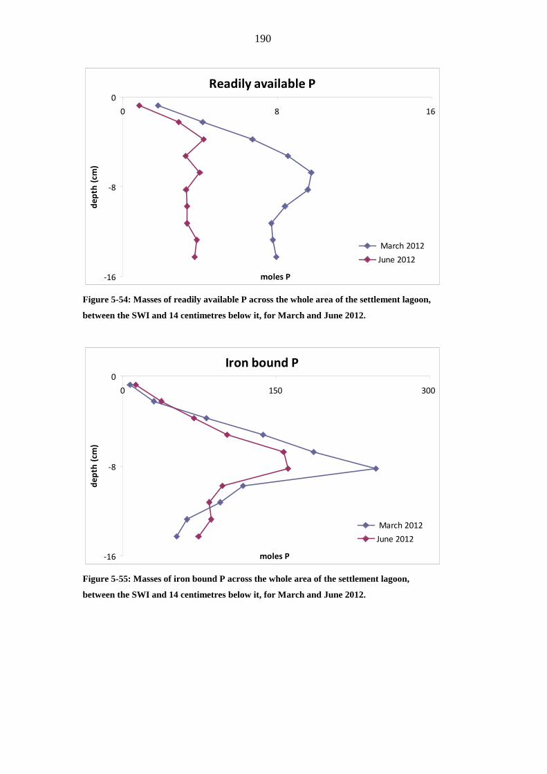
FIGURE 5-54: MASSES OF READILY AVAILABLE P ACROSS THE WHOLE AREA OF
THE SETTLEMENT LAGOON, BETWEEN THE SWI AND 14 CENTIMETRES
BELOW IT, FOR MARCH AND JUNE 2012..................................................................190
FIGURE 5-55: MASSES OF IRON BOUND P ACROSS THE WHOLE AREA OF THE
SETTLEMENT LAGOON, BETWEEN THE SWI AND 14 CENTIMETRES BELOW IT,
FOR MARCH AND JUNE 2012.......................................................................................190
FIGURE 5-56: MASSES OF APATITE P ACROSS THE WHOLE AREA OF THE
SETTLEMENT LAGOON, BETWEEN THE SWI AND 14 CENTIMETRES BELOW IT,
FOR MARCH AND JUNE 2012.......................................................................................191
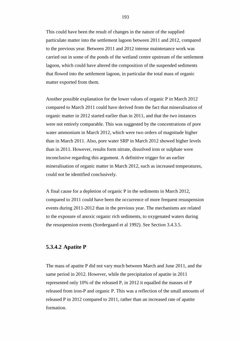
FIGURE 5-57: MASSES OF OTHER INORGANIC P ACROSS THE WHOLE AREA OF THE
SETTLEMENT LAGOON, BETWEEN THE SWI AND 14 CENTIMETRES BELOW IT,
FOR MARCH AND JUNE 2012.......................................................................................191
FIGURE 5-58: MASSES OF ORGANIC P ACROSS THE WHOLE AREA OF THE
SETTLEMENT LAGOON, BETWEEN THE SWI AND 14 CENTIMETRES BELOW IT,
FOR MARCH AND JUNE 2012.......................................................................................192
List of Tables
TABLE 1-1: SURFACE AREAS AND RETENTION TIMES OF THE DIFFERENT
COMPONENTS OF THE SOUTH FINGER WETLAND. ................................................32
Page 18
18
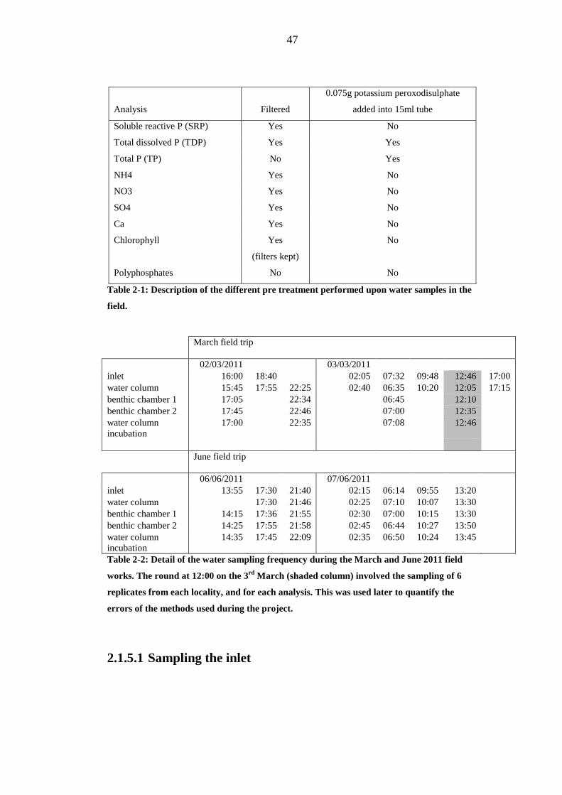
TABLE 2-1: DESCRIPTION OF THE DIFFERENT PRE TREATMENT PERFORMED UPON
WATER SAMPLES IN THE FIELD. .................................................................................47
TABLE 2-2: DETAIL OF THE WATER SAMPLING FREQUENCY DURING THE MARCH
AND JUNE 2011 FIELD WORKS. THE ROUND AT 12:00 ON THE 3RD MARCH
(SHADED COLUMN) INVOLVED THE SAMPLING OF 6 REPLICATES FROM
EACH LOCALITY, AND FOR EACH ANALYSIS. THIS WAS USED LATER TO
QUANTIFY THE ERRORS OF THE METHODS USED DURING THE PROJECT.......47
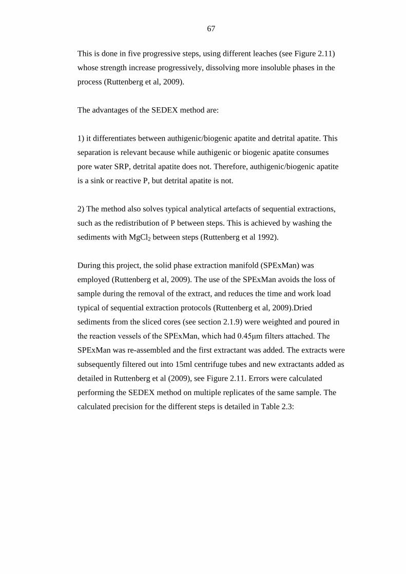
TABLE 2-3: CALCULATED ERRORS ON THE DIFFERENT STEPS OF THE SEDEX
METHOD ............................................................................................................................68
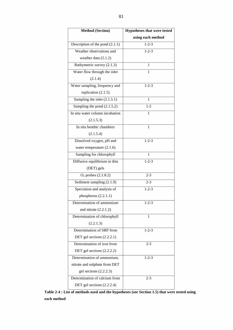
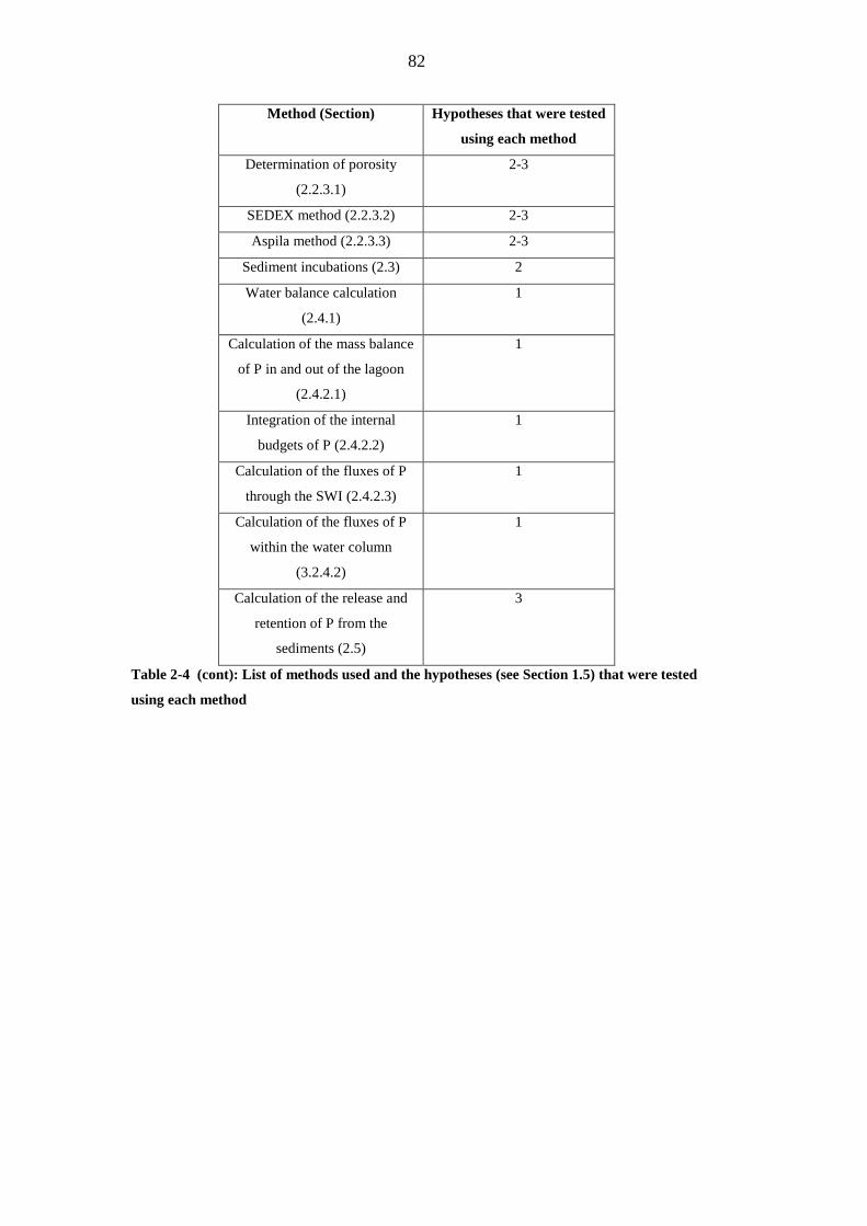
TABLE 2-4 : LIST OF METHODS USED AND THE HYPOTHESES (SEE SECTION 1.5)
THAT WERE TESTED USING EACH METHOD............................................................81
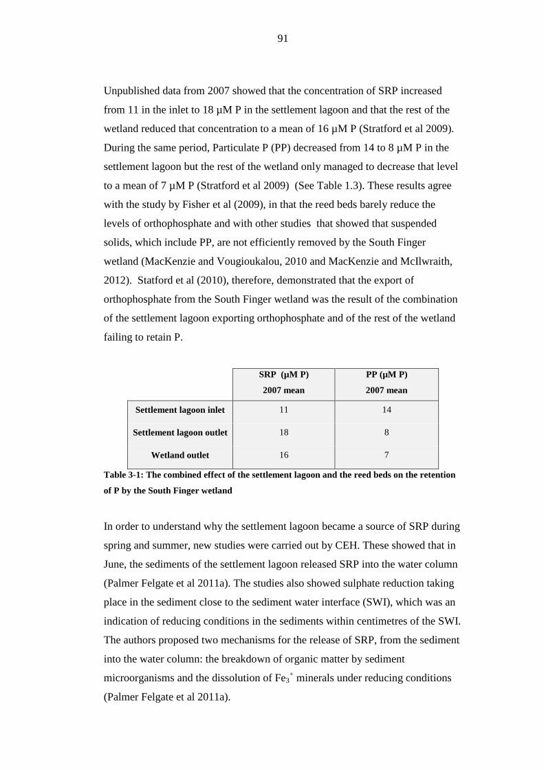
TABLE 3-1: THE COMBINED EFFECT OF THE SETTLEMENT LAGOON AND THE REED
BEDS ON THE RETENTION OF P BY THE SOUTH FINGER WETLAND..................91
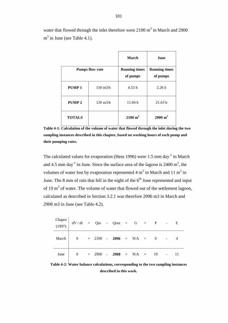
TABLE 4-1: CALCULATION OF THE VOLUME OF WATER THAT FLOWED THROUGH
THE INLET DURING THE TWO SAMPLING INSTANCES DESCRIBED IN THIS
CHAPTER, BASED ON WORKING HOURS OF EACH PUMP AND THEIR PUMPING
RATES...............................................................................................................................101
TABLE 4-2: WATER BALANCE CALCULATIONS, CORRESPONDING TO THE TWO
SAMPLING INSTANCES DESCRIBED IN THIS WORK. ............................................101
TABLE 5-1: MASS BALANCES OF THE DIFFERENT SPECIES OF P IN SEDIMENTS
BETWEEN MARCH AND JUNE 2011............................................................................188
TABLE 5-2: MASS BALANCES OF THE DIFFERENT SPECIES OF P IN SEDIMENTS
BETWEEN MARCH AND JUNE 2012............................................................................192
Page 19
19
1 Introduction
1.1 Treatment wetlands
1.1.1 Historical development
In Europe, waste waters started to be treated in the mid 1800s, coinciding with
the growth of big towns and cities with high population densities. Large towns
produced large quantities of waste waters harmful to the public health and to the
environment. The waste waters were not only domestic effluents, but they were
also generated in the many industries that used to be located within the cities,
such us slaughter houses, tanneries, printing presses, etc (Čížková 1998).
Originally, the treatment consisted simply of the disposal of waste waters onto
nearby lands. In the 1880s the treatment of waste waters became an industrial
process when biological filters were introduced, and by 1910 activated sludge
processes were developed. These last two processes rely on the consumption of
organic matter in the waste water by microorganisms, in an aerobic environment
(Čížková 1998). However, by 1950, European inland waters were being
impacted by the runoff from over fertilized farm land and from pollution from
sewage from decentralized small communities or industries, which was typically
treated in septic tanks or ponds, of low purification efficacy (Vymazal 2011,
Vymazal and Kröpfelová 2008). Dr Kathe Seidel started researching the use of
different species of macrophytes for the treatment of decentralised pollution in
Germany in the 1950s (Vymazal and Kröpfelová 2008). The research developed
into treatment wetlands, during which Dr Seidel tried different layouts, soil types,
plants species, etc (Vymazal and Kröpfelová 2008).
The advantages of the constructed wetlands were their low cost of construction
and operation, but their rate of treatment was slower than conventional
wastewater treatment technology. Constructed wetlands were shown to be well
suited for treating effluents from small communities or as a final polishing step
Page 20
20
of previously treated water from larger population centres. There was however
scepticism from water treatment experts, who would not accept that macrophytes
would grow well in polluted waters and that they would not be able to eliminate
toxic substances (Sidel 1976). There were many prejudices among civil
engineers about the viability of running constructed wetlands, for example
regarding the production of odours and flies and their poor performances in cold
weather (Veenstra 1998).
The first constructed wetlands were commissioned in the Netherlands in 1967,
and in Hungary in 1968 to process pre treated waste water. In the US, the use of
constructed wetlands also started in the 1960s for the treatment of municipal
waste water (Vymazal 2011). Currently there are thousands of constructed
wetlands around the world that treat municipal and industrial waste waters,
agricultural runoff, mine drainage and storm waters (e.g. Dunbabin and Bowmer
1992, and Maynard et al 2009). In the UK, the Water Authority and the Water
Research Centre investigated constructed wetland systems operating in Denmark
in 1985, and by the end of that year the first constructed wetland was in operation
in Britain. By the end of the century, there were probably 400 to 600 privately
owned constructed wetlands in the UK, plus another 150 owned and operated by
Severn Trent Water (Čížková 1998).
1.1.2 Free water surface constructed wetlands
There are different types of constructed wetlands that vary, for example, on
whether water flows above or below the surface of the sediments, or whether
plants are attached to the sediments or floating (See Figure 1.1). In this
introduction and throughout the thesis, the free water surface (FWS) type of
wetland will be discussed. FWS wetlands consist of a basin or number of
interconnected basins filled with 20 to 30 cm of organic rich soil. They are
typically planted densely with emerging macrophytes, in addition to other
naturally transplanted species (Kadlec and Hey 1994). Water flows over the soil
and around the emerging plants at depths between 20 and 40 cm (Vimazal 2011).
The water should cover all parts of the wetland to maximise the use of all the
Page 21
21
available surfaces for the chemical and biological reactions that will treat the
water (Kadlec and Knight 1996). This is usually achieved by designing the
basins as long and narrow channels (Reed et al 1998). Sedimentation of heavier
particles occurs in the first few meters from the inlet. Vegetation reduces the
water column mixing and the resuspension of particles from the sediments,
allowing the settling of lighter particles that did not settle near the inlet (Čížková
1998).
Microorganisms are responsible for the removal of soluble organic compounds,
which are mineralised both aerobically and anaerobically. Aerobic
microorganisms are very effective in the breakdown of organic matter carried in
the waste water, whereas anaerobic microorganisms also facilitate the breakdown
of organic matter, but at slower rates (Shutes 2001). The decomposition of
organic matter then will depend largely on the supply of oxygen to the waters
and to the sediments. Oxygen is supplied to the shallow water column by
diffusion through the water surface and also by photosynthesis mainly on the
periphyton and by benthic algae (Kadlec et al 2000). Oxygen is supplied to the
sediments through the emerging plants. Plants of large biomass, that grow in
water saturated soils and that have an extensive root system are most commonly
used in constructed wetlands. These usually are common reed (Phragmaites
australis), and reedmace (Typha latifolia). The oxygen that the plants draw from
the leaves down to the roots creates an area within the soil (the rhizosphere) that
can sustain aerobic microorganisms (Shutes 2001).
The removal of nitrogen from FWS systems by the harvesting of plants is
minimal, since the mass of N removed during an annual harvest is a small
fraction of the total mass of N that has to be removed during one year from
typical waste waters. Instead, N is mainly removed by nitrification/denitrification,
and volatilisation. These processes are triggered when ammonium is oxidised to
nitrate, in the presence of oxygen; and nitrate is used up by denitrifiers. FWS
wetlands are typically oxygenated near the water surface and around the
rhizosphere and ammonium is oxidised to nitrate in those aerobic zones by
nitrification (Vymazal 2011). In turn, in anaerobic areas, the high organic content
Page 22
22
of the waste water and the plant litter fuels denitrification. Finally elemental N
and nitrous oxide are volatilised (Huang and Pant 2009).
FWS constructed wetlands can also remove disease-bearing microorganisms.
This is achieved by a combination of processes such as filtration, exposure to UV
radiation, sedimentation and oxidation. Many biological processes also occur that
would destroy pathogenic organisms such as the excretion of biocides by some
plants, predation by other microorganism and natural senescence (Gersberg et al
1987).
Page 23
23
a)
b)
c)
d)
OutflowInflow
OutflowInflow
Water
Outflow
Inflow
Water
Soil
Weir
Weir
Elbow pipe
Saturatedsediment
Drysediment
Waterlevel
Perforated pipe
Inflow
Outflow
Wetsediment
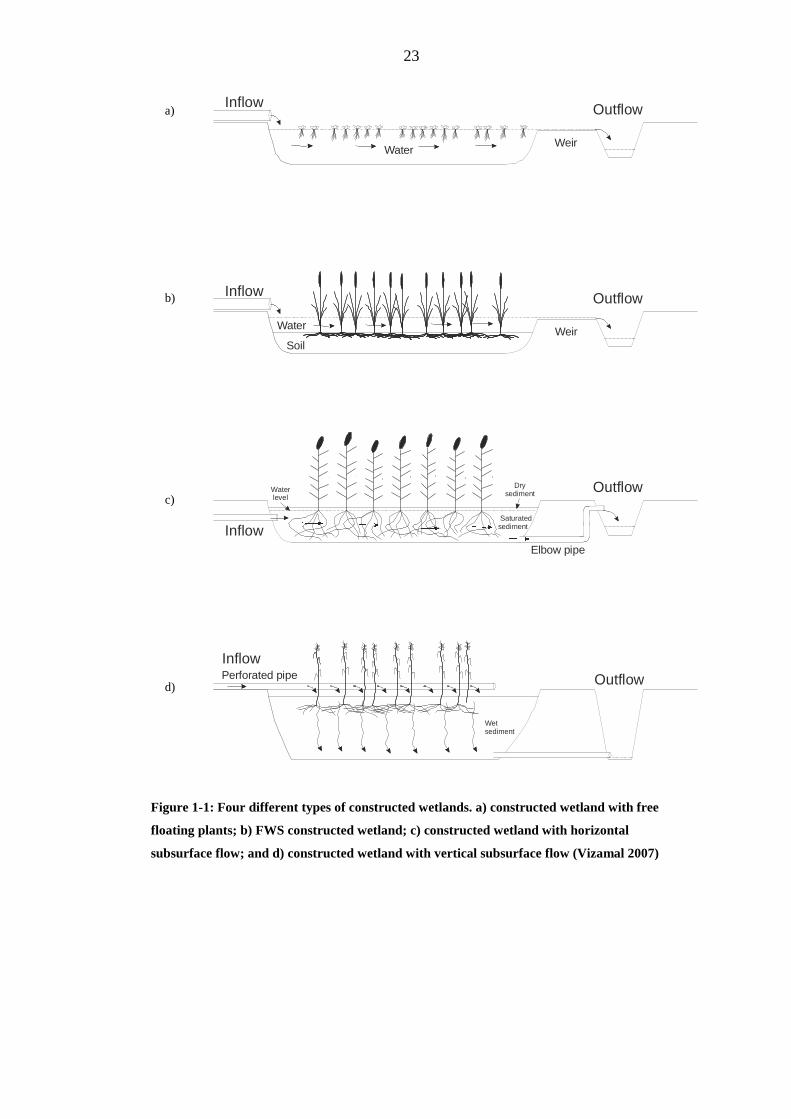
Figure 1-1: Four different types of constructed wetlands. a) constructed wetland with free
floating plants; b) FWS constructed wetland; c) constructed wetland with horizontal
subsurface flow; and d) constructed wetland with vertical subsurface flow (Vizamal 2007)
Page 24
24
1.1.3 The retention of phosphorus by FWS constructed
wetlands
The long term retention of phosphorus (P) by constructed wetlands is the result
of physical, chemical and biological processes (Reddy et al 1999). These can be
summarised as the accretion of plant litter containing P, sorption of P into pre-
existing minerals and storage in biomass (Kadlec and Knight, 1996). Only the
first process is sustainable, while the other two processes reach saturation and
therefore cannot give a long term solution for the retention of P (Dunne and
Reddy, 2005). Even the physical retention of P by accretion of detrital material in
the wetland floor will depend on the P content of the litter, which is usually low
(Reddy et al 1999) and on the capacity of the wetland to accumulate litter, which
can be sustained by management of the wetland. Detritus laying on the floor of
wetlands have lost up to 80% of the mass of P that the living plants originally
held (Reddy et al 1999).
P adsorbs onto mineral surfaces, typically Al and Fe oxides, and with time it
diffuses into the mineral lattice via absorption, but the processes are slow and Fe
minerals have a limited capacity to absorb P (Reddy et al 1999). These processes
are more efficient in soils with a higher inorganic fraction and in wetlands where
water flows through the sediment instead than over the sediment surface.
Subsurface flow wetlands (see Figure 1, c) and d) ) therefore are efficient in the
removal of P through adsorption-absorption mechanisms. Changing conditions of
a constructed wetland may affect these processes. If the water column went
anoxic, the sediment water interface (SWI) would also go anoxic and in reduced,
anaerobic conditions, ferric iron would reduce to soluble ferrous iron, releasing
previously bound P into the water column (Mortimer, 1941).
Co-precipitation is the combination of P with some metallic ions forming
amorphous or poorly crystalline solids. The co-precipitation with Ca2+ ions is
generally important in wetland soils at pH values higher than 7 (Faulkner and
Richardson, 1989). Co-precipitation of P with Ca2+ taking place in FWS
Page 25
25
wetlands results in authigenic apatite, which once precipitated is a permanent
sink of P at pH values above 4 (Ruttenberg 1992).
In the water column, planktonic algae and microbial uptake can remove
phosphorus rapidly, but the mass of P removed is low (Vimazal 2007), and P is
rapidly remobilised from their detritus into the water column (Vymazal 2011).
Planktonic algae and bacteria can also affect the retention of P indirectly by
changing oxygen levels and pH through photosynthesis and respiration (Gachter
and Meyer 1993). This affects mechanisms of P sorption into Fe minerals
described above.
Soil bacteria can facilitate the burial of P by the production of refractory
compounds rich in P, such as polyphosphates (Poly-P) (Gachter and Meyer 1993).
However, they can also mobilise stored P directly by decomposing buried
organic matter and releasing nutrients, and indirectly by changing redox
conditions, which would affect sorption onto Fe minerals (Vimazal 2007). It has
been suggested that microorganisms mediate in the precipitation of insoluble
calcium-P minerals in the oceans, through the production of polyphosphates
(Poly-P), that subsequently act as nucleus for the precipitation of authigenic
apatite (Diaz et al 2008), but no study has been found of this process taking place
in constructed wetlands. As with nitrogen, P removal by harvesting the emerging
macrophytes is low (10 to 20 g P m-2 y-1) when compared with the influx of P
typical in treatment wetlands, which is typically one order of magnitude higher
(Vimazal 2007).
1.2 The Slimbridge Wetlands Centre
1.2.1 Site history and description
The UK has a long history of nature conservation that dates back to the 1870s,
when living conditions in the cities and evident damage caused in the countryside
led to an increasing number of people to start discussing their behaviour towards
Page 26
26
the natural world. In 1891 the Royal Society for the Protection of Birds was
founded, and the idea of natural reserves was introduced by its members in the
early 1900s. By 1930, The National Trust, the Royal Society for Nature
Conservation, the British Ecological Society, and the Forestry Commission were
already very active. Popular claim for public access to the countryside increased
in the 1930s. In 1932 an organised mass trespassing on private land took place in
the Peak District. These acts and pressure from the different conservation
societies forced parliament to pass a series of laws that would culminate in the
1949 National Parks and Access to the Countryside Act (Evans, 1992).
As part of this nature conservation movement, a naturalist called Peter Scott
inaugurated the Severn Wildfowl Trust, in 1946, which occupied seven hectares
of natural wetland on the banks of the river Severn, in Slimbridge, Gloustershire.
The Trust was the most successful of the post war conservation organisations
created in Britain and led to similar trusts for the conservation of pheasants,
hawks, etc (Fitter and Scott 1978). The Severn Wildfowl Trust was created as an
observation and research centre, dedicated to the study of a captive collection of
waterfowl and to the study of wintering wildfowl on the Severn estuary. The
Wildfowl Trust became a success with the public immediately after creation, and
its educational value has been as important as the value of its scientific research.
The Trust has worked extensively in practical conservation, by creating new
wetlands habitats and by breeding endangered species in captivity and
reintroducing them to the wild in different parts of the world. The Severn
Wildfowl Trust opened other centres in the UK and in America and in 1989 the
trust changed its name to Wildfowl and Wetlands Trust (WWT) (Evans 1992).
The WWT site in Slimbridge now extends to 325 hectares, of which 50 hectares
belong to the Visitor Centre and to the ponds where the captive collection is kept,
and the rest is wild marshland. The site has been designated a Special Protection
Area and a Special Area of Conservation according to Directives of the European
Union, and as a Ramsar Site (McKenzie, 2010). The Visitor Centre (see Figure
1.2) is surrounded by marshland and agricultural land and it lies between the
Gloucester and Sharpness canal and the river Severn. Water from the canal and
from adjacent farmland enters the Visitor Centre and flows through several
Page 27
27
interconnected ponds. The ponds are the habitat for the captive collection and for
migrating wild birds. The permanent population of birds living on the ponds is
2000 wildfowl in summer, but it rises to 3000 when the migrating birds arrive in
the winter months (Mckenzie and Vougioukalou 2010). The high density of birds
living at the Visitor Centre affected the quality of the water flowing through the
exhibit ponds, mainly as the result of uneaten feed and bird faeces. This caused
relatively high suspended solids, biological oxygen demand, ammonia and
phosphate (Mckenzie and McIlwraith 2012). This problem is common in water
leaving bird reserves (Manny et al 1994). In 1994, the South Finger treatment
wetland was installed downstream of the exhibit ponds to treat the out flowing
waters before they reached sensitive areas of the River Severn.
Figure 1-2: Layout of the WWT site, showing the SouthFinger Wetland. The ponds are
interconnected (not all connections shown) and they discharge in the ditch immediately
upstream of the South Finger Wetland.
Page 28
28
1.2.2 The South Finger Treatment Wetland
1.2.2.1 Construction of the South Finger treatment wetland
In 1991, WWT commissioned the environmental consultancy Penny Anderson
Associates to produce a draft outline for the construction of a treatment wetland
that would clean effectively the water flowing out of the visitor centre and
exhibit ponds (Millett, 1997). The objectives that WWT gave to the consultants
for the design of the constructed wetland were (Mackenzie, unpublished draft).
• To meet the discharge consent levels
• To produce water that would meet nature conservation standards
• To combine the treatment of water with the creation of habitats for nature
conservation
• To create an educational site
These objectives were developed into six broad approaches (Worral, 1997):
• Suspended solids would be encouraged to settle using ponds that would
force the reduction of energy (velocity) of the inflowing particles
• The wetland would be of the FWS type, described in sections 1.1.2 and
1.1.3
• Cascades made of limestone would be used along the FWS wetland to
encourage the aeration of the water and to promote the co-precipitation of
P with Ca2+ (see section 1.1.3)
• Floating rafts would be deployed on the ponds to assist the treatment
process
• Different types of plants would be used, to promote diversify and to avoid
the failure of the whole system in case of the failing of one species of
plants
• Wetland habitats would be created to mimic natural ones and to promote
wildlife
Page 29
29
In 1993 the wetland was excavated on a field used for cattle grazing next to the
visitor centre. The excavated clays were used by the Environmental Agency (EA)
to improve sea defences nearby. That meant that the costs of the excavation were
covered by the EA and also that lining of the wetland was not needed because the
wetland had a clay base. The treatment wetland was finished in 1994, when
funds were finally raised to cover the costs for pumps and plants (Mackenzie,
unpublished draft).
1.2.2.2 Layout and operation of the South Finger treatment
wetland
The layout of the South Finger treatment wetland can be seen in Figure 1.3. The
individual sections of the wetland and their operation are described below:
Inflow
Settlementlagoon
Harvest bed
Iris bedMosaic bed
Phragmites bed
Floatingrafts Lagoon 2
Chalkcascade
Scirpus bed
Phragmites
bed
Outflow
0 10 50 100 mts
N
Figure 1-3: Layout of the South Finger treatment wetland, at the Wildfowl and Wetland
Trust’s site in Slimbridge.
Water leaving the exhibit ponds is collected in a ditch between the visitor centre
and the wetland. The ditch has a lateral connection to a concrete pumping
chamber. There is a weir in the ditch, just downstream of the pumping chamber
to keep water levels high. This ensures that water reaches the right depth to
trigger the pumps inside the chamber. During unusual high flow conditions, for
example after a storm, excess water that cannot be taken up by the pumps runs
Page 30
30
above the weir and flows untreated along a lateral ditch. A high level switch in
the chamber is triggered when water levels rise in the ditch. The switch starts up
the pumps within the chamber and these pump water from the chamber and the
ditch into the settlement lagoon. The pumps stop automatically when a low level
switch is triggered. There are two pumps inside the concrete chambers that are
usually run alternately (Mckenzie and McIlwraith, 2012).
Settlement Lagoon
The settlement lagoon was originally 1.5 meters deep, and could hold a volume
of approximately 2900m3. The water flow was 2000 m3 day-1, resulting in a
residence time, when constructed, of 35 hours. The settlement lagoon was
designed to slow the velocity of the suspended solids contained in the inflowing
water, and to make them settle on the bottom. The settlement lagoon was to be
allowed to fill with sediments, which was expected to take 25 years. After that it
would be converted into a reed bed or re-excavated (Millet 1997).
Harvest Bed
The harvest bed was designed to treat water from the settlement lagoon before
flowing into the Iris bed. However the connection between the harvest bed and
the Iris bed has never been established. Alternatively, the harvest bed has been
used as a nursery for wetland plants (Mackenzie and McIlwraith, 2012) and to
provide reed material needed for filters around the WWT site (Millet 1997).
The Treatment Beds
The treatment beds are of the FWS type, described in sections 1.1.2 and 1.1.3
above. This type of flow was chosen because it provides good habitat for wildlife
and because of its ability to treat large volumes of water. The beds can be
individually isolated for maintenance work (Millett 1997).
Floating Rafts Lagoon
Page 31
31
The surface of this lagoon is almost all covered by rafts. The rafts had a mesh to
hold several species of aquatic plants. The roots of the plants hang through the
meshes into the water column. Microorganisms living on the root surfaces treat
the water further (Millet 1997), as discussed in 1.1.2.
Chalk Cascade
The cascade is made of crushed limestone, covered with chalk. The turbulence of
the water flowing over the cascade promotes oxygenation of the water. The
materials for the construction of the cascade were chosen to promote the co-
precipitation of P with Ca2+ ions (Millet 1997), and as described in 1.1.3.
However, the surface of the stones soon became covered by algae, suppressing
the co-precipitation of P (Worral et al 1997).
Scirpus and Phragmites beds
They operate similarly as the treatment beds, but they were excavated deeper in
the clay to allow a longer contact between the water and the sediments, in order
to promote the capture of P by the sediments (Millet 1997), as discussed in 1.1.3.
From the settlement lagoon, water flows by gravity down to the outlet of the
wetland. Water flows out of the settlement lagoon when it reaches the level of
three elbow-bend pipes. These three pipes are connected below ground to the
three treatment beds (Iris, Mosaic and Phragmites). Water levels in the treatment
beds are maintained by brick weirs built at the exit of the inflowing pipes and by
elbow-bend pipes at the other end of the beds (See Figure 4). Water from the
treatment beds run below ground through pipes into the Floating Rafts Lagoon.
The inlets into the Floating Rafts Lagoon are below the water level. Downstream
of the Floating Rafts Lagoon there is a chalk cascade, over which the water flows
into the Lagoon 2. As with the settlement lagoon, elbow-bend pipes in the
Lagoon 2 drive the water into the last two smaller treatment beds (Scirpus and
Phragmites). Water exits the wetland through pipes under a track and into a ditch.
This ditch, or rhine, discharges eventually into the river Severn, 500 meters .
Page 32
32
Settlemnt
lagoonTreatment beds
Rafted
lagoon
Cascade
lagoonPolishing beds
Phrag
mitesMixed Iris Phragmites Scirpus
Area
(m2)2900 1725 2250 2000 550 950 1300 1000
Design
Retention
Time (hs)
35 6 8 7 6 11 2.4 3.1
Table 1-1: Surface areas and retention times of the different components of the South
Finger wetland.
1.2.3 Retention of P by the South Finger wetland
Research undertaken on the South Finger wetland demonstrated that the wetland
has been exporting orthophosphate every year since 2005, and possibly since
1996. The source of the excess orthophosphate is the settlement lagoon, while the
rest of the constructed wetland has been unable to reduce the excessive fluxes
(Stratford et al, 2010 and Palmer-Felgate, 2011a and 2011b. Observations similar
to those made at the settlement lagoon have been reported in shallow lakes. For
example Lake Blankensee in Germany has an average depth of 1.2 meters, and
the majority of the TP in the water column in summer was reported to be
generated within the lake (Ramm and Scheps 1997). Loch Leven in Scotland has
a mean depth of 3.9 meters and an area of 13.3 km2. Water column SRP is
depleted in spring due to the uptake of the spring algal blooms, while in late
summer the peaks are produced by intense release from the sediments (Spears et
al 2007). Further examples of shallow lakes that release phosphorus internally
are given from lakes in Denmark (Søndergaard et al 2003), Sweden (Ryding
1985), Italy and the US, (Marsden 1989).
1.2.3.1 The settlement lagoon as the source of excess P
As discussed above, the settlement lagoon is the source of excess P within the
South Finger wetland. P cycling in such shallow bodies of water has some
Page 33
33
characteristics that differentiate them from deeper stratified lakes. Given the
surface area to depth ratios of shallow lakes, the pool of P in the sediments is
often more than 2 orders of magnitude larger than the pool of P in the water
column. Therefore the levels of P in the latter depend largely on the fluxes
through the SWI (Søndergaard et al 2003). Lake Ontario, in North America, has
a mean depth of 89 meters, and the internal loading of P has been estimated to be
11% of the external load. On the other hand, in a number of shallow lakes in
Sweden, the internal load of P is up to 4 times larger than all other external loads,
averaged annually (Boström et al 1988a). The passage of P from the sediments
into the layers in the water column where photosynthesis takes place is rapid and
direct (Shaw and Prepas, 1990; Søndergaard et al 2003), therefore it has a critical
impact on the primary productivity in the water column (Boström and Pettersson
1982).
The release of P from the sediments in shallow lakes happens mainly from
aerobic sediments (Jensen et al 1992, Marsden 1989), and the rates of release
from sediments in well oxygenated waters are often of the same magnitude as for
anaerobic sediments (Boström et al 1988a). This disagrees with the classical
model of Mortimer (1941) for deep lakes, but the inherent characteristics of
shallow lakes help explain this:
freshly produced organic matter in shallow lakes reaches the sediment
surface quickly and almost intact
the water column is subject to rapid changes in its physical and chemical
conditions
resuspension events are frequent
Large amounts of freshly produced organic matter falls onto the sediments of
shallow lakes before decomposing. This is a rich source of organic matter for
sediment microorganisms, which have a significant role in the uptake, storage
and release of P, as long as the oxygen levels and other oxidisers like nitrate are
present (Søndergaard et al 2003). It has been reported that in shallow lakes, up to
50% of the primary production is mineralised in the bottom waters or in the
Page 34
34
sediments (Caraco et al 1990). Release of P originated from the decomposition of
algae on the sediments surface of Lake Grevelingen and from the Loosdrecht
Lakes in the Netherlands (Marsden, 1989). Mass balance calculations indicated
that the release of SRP occurred on the top few centimetres of sediments, and it
has been suggested that the P loading of the lakes was caused by the
mineralisation of organic matter (Marsden, 1989). An additional effect of high
concentrations of SRP near the sediment surface is that they lower the Fe:P ratios
in those top layers, and it has been suggested that at Fe:P ratios below 15,
orthophosphate would cross the oxic layer into the water column without being
adsorbed by iron minerals (Jensen et al 1992, and Ramm and Scheps 1997).
Sediments in shallow lakes are exposed to more heterogeneous conditions than in
deep lakes, because of the combined effects of weather, the circulation of water,
shelter from nearby trees, buildings and fauna (Boström et al 1988a). That
heterogeneity causes the formation and destruction of micro chemical gradients
in the sediments and in the pore waters, related to temperature, pH or levels of
oxygen (Boström et al 1988a). The chemical gradients change rapidly and
unpredictably, and loosely-bound P or P in solution in the pore waters are
continuously recycled into and out of the water column (Boström and Pettersson
1982) and wide variations in the release of P can occur in shallow lakes
(Marsden 1989). Water column and sediment temperature in shallow lakes can
span 20°C rapidly. This causes great variations in the rates of microbial activity
and the releases of P associated with it (Sinke et al 1990). An increase in primary
productivity, resulting from changing environmental conditions, causes an
increase in pH (Sinke etal 1990) and higher pH trigger the release of
orthophosphate from sediments, by ion exchange between OH- and PO43- on the
surfaces of Fe oxy-hydroxides (Jensen and Andersen, 1992). Although the water
column of shallow lakes is usually well mixed and oxygenated (Søndergaard et al
2003), it has been reported that under special weather conditions in summer,
anoxia can set in the top millimetres of the sediments (Shaw and Prepas, 1990),
or that even the water column can become anoxic overnight during warm and
calm weather (Correll 1998). When this occurs, P stored in the oxic top
millimetres of the sediments can be liberated as Fe minerals are chemically and
microbially reduced (Søndergaard et al, 2003).
Page 35
35
It has been reported that in shallow lakes, the top 10 cm of sediments can be
subject to disturbance and mixing by water turbulence (Forsberg 1989), and that
the release of dissolved P from pore waters after the resuspension of sediments or
the mineralisation of resuspended sediments is significant (Boström et al 1988b).
Also, the constant turbulence in the water column maintains steep concentration
gradients between the SWI and the overlying water, accelerating the process of
molecular diffusion between the two phases (Forsberg 1989). A shallow lake in
Denmark showed increases of between 5 to 10 times the background levels of TP
in the water column within days of high wind events (Søndergaard et al 2003).
The same authors discussed that yearly variations in the internal P loading in
other shallow lakes were controlled by wind mixing (Søndergaard et al 2003).
Internal P loading of Lake Blankensee in Germany was also shown to be the
result, in part, of disturbance of sediments by water turbulence (Ramm and
Scheps 1997).
1.3 Aims of research, hypotheses and structure of the
thesis
This project is part of WWT’s plan to develop an understanding on the
performance of the South Finger wetland, primarily regarding the retention of P.
This project builds on the findings of Stratford et al (2010) and Palmer-Felgate
(2011a and 2011b), who studied the retention or release of P by the South Finger
wetland in the past. Their work indicated that the wetland exports orthophosphate,
and that its source is the settlement lagoon, and they measured and suggested
possible mechanisms for the release of P from the settlement lagoon. However,
the proposed mechanisms were not quantified or studied in depth.
The general aim of this research project was to quantify and to understand in
depth the mechanisms that resulted in the settlement lagoon exporting P. This
was carried out by testing three main hypotheses, which are based on the likely
behaviour of P in a body of water like the settlement lagoon (see Section 1.2.5):
Page 36
36
1. The sediments are the source of excess P that is discharged from the
settlement lagoon in summer. The discussion of this hypothesis was
presented in Chapter 4.
2. P released from the sediments in summer resulted mainly from the
mineralisation of organic matter, and it was triggered by the increase in
temperatures. This hypothesis was discussed in Chapter 5.
3. The organic matter that releases P is the combination of freshly deposited
primary productivity and of bird faeces that accumulated in the sediments
during the previous year. This hypothesis was discussed in Chapter 5.
The historical performance of the settlement lagoon regarding P is presented in
chapter 3. Chapter 6 includes a summary of the previous three chapters and
Chapter 7 presents the conclusions and implications of the study presented in this
thesis.
1.4 Relevance of the proposed study
The study of nutrient cycling and its effect on eutrophication of surface waters
commenced in the 1900s and it is still intense, due to its relevance on water
quality and management (Smith et al, 2003). In the last 40 years there has been a
significant increase in the research of nutrient cycling, and many improvements
have been made in order to prevent excessive N and P entering lakes, rivers and
the sea. However, eutrophication continues to be one of the main problems in
protecting our waters resources (Smith et al, 2003). Mainstone and Parr (2002)
discussed in depth the mechanisms in which the introduction of reactive P in the
water environment degrades the environment. The authors concluded that P in
surface water systems should be brought back as close to background levels as
possible. The negative effect of P in the water quality of surface waters is related
with an increase in algal growth and production of organic matter. However,
even this aspect of the research on eutrophication has been questioned recently.
Hagerby et al (2006) concluded that in some instances high nutrients loadings
Page 37
37
cause a decrease in productivity, indicating that the subject of euthrophication is
far of having been fully understood. In the proposed work, nutrient levels and
chlorophyll levels in the water column will be presented and their relationships,
discussed.
A possible way of understanding the cycling of P in lakes is by estimating its
loads and budgets, and by investigating internal nutrient dynamics and retention
mechanisms. This approach was presented in Tang and Xie (2000), and it is also
an important part of the proposed study. More complex models have been also
applied to the study of nutrient cycling in lakes and these are being developed
and improved constantly, for example the DYRESM–CAEDYM model
described in Trolle et al (2008). Correlations between levels of nutrients,
chlorophyll levels, transparency, solids in the water, weather and the time of the
year were also discussed by James et al (2009), as well as in the proposed work.
The research presented in this thesis includes the study of the cycling of organic
P, both in the sediments and in the water column. This species of P has not been
studied in depth in the past and is currently a subject of intense research
(McMahon and Read, 2013). The complexities of the relationships between
living organisms, decomposing organisms and different species of organic P,
such as polyphosphates, pyrophosphates, orthophosphates monoesters and others
are discussed in detail in, for example, Reitzel et al (2007). The subject of
organic species of P is among the latest areas of research in the water treatment
industry, where microorganisms are manipulated to accumulate P from waste
waters (McMahon and Read, 2013). The interactions of these organic species of
P and of the phosphorus accumulating organisms, with other chemical species
have also been investigated, in order to optimise the performance of water
treatment plants (Saito et al, 2004, Saito et al, 2008, and Jie et al 2007). These
studies have been complemented with techniques developed to enrich the culture
of phosphate accumulated organisms in water treatment plants, in order to
enhance the biological removal of phosphorus from waste waters (Hung et al,
2002). Novel methods for the quantification of organic species of P and of P
accumulating organisms have also been developed recently (e.g. Aschar-Sobbi et
al, 2008; Hupfer et al, 2008 and Diaz and Ingall, 2010).
Page 38
38
The fate of P when it reaches the sediments has been studied for many decades
(e.g. Mortimer, 1941), and the topic is still subject to intense research. This is in
part because of its complexity, but also because the burial and release of P from
lake sediments continue to impact the quality of surface waters (Mesnage et al,
2002), even well after loading of P has stopped (Reitzel et al, 2012). Different
aspects of the cycling of P in lake sediments that have been being studied for the
last 50-60 years are still being investigated. These include, among others, the
effects of light and mechanical perturbation of sediments over the release and
uptake of phosphorus from sediments (Gerhardt et al, 2010); or the relationships
between water column processes, phosphorus release or uptake from sediments,
and sediments types (Vicente et al, 2006), or the optimisation of classical
methods (Kapanen, 2008) such as those presented in Hieltjes and Lijklema
(1980) and Murphy & Riley (1962), for the study of sediment phosphorus. Many
of these topics are discussed in the proposed work.
The interactions between sediments and water column P is still a relevant issue in
modern research of lakes, and many of those characteristics are discussed in the
proposed study. Resuspension events in shallow lakes and their effect on water
column P have been studied in Holmroos et al (2009), and it was shown that
those events can increase considerably the concentrations of TP and SRP in the
water column. However, it was discussed that resuspension events can either
release dissolved P into the water column or sequester dissolved P from the water
column. The conditions for the different behaviors are related to the volume of
water that reacts with the resuspended sediment, oxic conditions and pH (Koshi-
Vähälä and Hartikainen, 2001). The effect of benthic fauna in the release of
nutrients and turbidity of lakes is still a debatable subject, as was discussed in
Torvainen et al (2005). That study obtained results that seemed to contradict
previous ones, for example those which showed that chironomids (vulg. Blood
worms) do affect turbidity of the overlying water but they do not impact the
levels of P in the water column (Torvainen et al, 2005).
The impact of waterfowl on surface waters is a current matter of concern for lake
and wetlands managers and many questions regarding this issue are currently
Page 39
39
being studied. For example what is a sustainable population of birds? How to
measure this? What are the direct and indirect impacts of bird populations of
surface waters? (Chaichana et al, 2010, and Huang and Isobe, 2012). Some of
these questions are studied thoroughly in the present work and contributed to the
study of this important environmental issue.
The remediation of waters impacted by high levels of nutrients using constructed
wetlands continues to be studied intensely. For example Venterink et al (2002)
focused on the consequences that well established practices have on the release
and bioavailability of P. The authors concluded that the common practice of
flooding land to create artificial wetlands could in fact release large masses of P.
The performance of treatment wetlands has often been unsatisfactory regarding
the retention of P and the issue has been subject to recent research. For example,
Stottmeister et al (2003) gave a comprehensive description of how plants and
microorganisms affect the removal of nutrients from the polluted waters.
The proposed work is a contribution to the ongoing research, and contributes
specially in the understanding of P cycling and measuring of fluxes of P in an
organic rich aquatic system. In general, treatment wetlands contain inflowing
reactive P for a short period of time before becoming saturated. For example Jin
et al (2001) described very good results regarding retention of reactive P, in a
series of pilot tests. However, Braskerud et al (2005) demonstrated that wetlands
rapidly lose their capacity to contain reactive P, and that the settling of
particulate P becomes their main form of P retention. Similar findings were
reported in Braskerud (2002). Toet et al (2005) proved that a treatment wetland
used to polish effluent from a sewage treatment plant succeeded in reducig the
mass of P by only 5%. Concordantly, Scholz et al (2007) describes the design of
treatment wetlands treating runoff form farmyards. The authors reported long
term good performances of treatment wetlands, regarding P, when those were 1.3
to 1.4 times the surface area of the farmyard. However, these types of ratios
between the wetland and the catchment area are impractical when the catchment
is ten or hundreds of hectares, like the WWT site at Slimbridge.
Page 40
40
The proposed research is focused on the settlement lagoon of a treatment wetland.
In Peng et al (2007), it is discussed that wastewater stabilisation ponds have been
understudied in the past and the interest in the cycling of nutrients in them has
become more relevant as the use of stabilisation ponds for non-point pollution
increased. That same study described how different forms of particulate P are
more or less stable under different pH and redox conditions. Wastewater
stabilisation ponds have also been recently studied as habitats that favour the
luxury uptake of phosphorus by algae, as a mean or removing reactive P. The
main factor favouring luxury uptake of P was concluded to be temperature, rather
than light (Powell et al, 2008).
Page 41
41
2 METHODS
This chapter describes the general field and analytical methods employed during
this project. The rationale of why these methods were employed and other more
specific methods are elaborated in detail in subsequent chapters.
2.1 Field methods
2.1.1 Description of the pond
The great majority of the field work was done in the settlement pond. The shape
of the pond can be described as a quarter of a circle of radius 50m. That equates
to a surface area of approximately 2000m2. The original depth of the pond was
between 1.5 and 2 meters excavated in natural stiff clays, with a shallower shelf
left to the south of the pond (Millett, 1997). Settling of solids has caused these
depths to decrease through the years, and it has been reported that the current
depths of the pond are 0.6 to 1 meter. The fresh sediments are very soft and dark
grey to black in colour, with a reported mean LOI of 13.5 % (Palmer Felgate et al
2010). It has also been reported that there is a thick transition layer between the
sediment and the water column (Palmer Felgate et al 2010). Typical H2S smell
and intense bubbling occurred when the sediments were disturbed.
In June 2011 a small stickleback was found floating dead in the water, suggesting
the existence of a fish population in the pond, although live fish were not seen.
The bottom of the pond is unvegetated but its edges are vegetated largely by
Reedmace (Typha Latifolia), which has crept up to 3 meters into the pond. There
are four rafts of about 1 square meter each, secured to the bottom of the pond
(see Figure 2.2). Some vegetation grows on the rafts with their roots suspended
inside the water column. In summer, a few floating macrophytes were observed
but they were not identified.
Page 42
42
The inlet pipe is to the north of the settlement pond and it is fed by centrifuge
pumps that bring the waste water from the bird collections upstream. Three outlet
pipes drain the pond by gravity when the water level reaches them (see Figure
2.1). The water is likely have a short residence time if it flows along the western
half of the pond. On the other hand, water left in the eastern half of the pond will
have an extended residence time until it reaches the outlets (Hossain et al 2005).
Inlet
Outlet
OutletOutlet
North
50 meters
Site 1Site 2
Figure 2-1: Plan view of the settlement pond at the South Finger constructed wetland, with
detail of positions of inlets, outlets and sampling points 1 and 2.
The sampling of the pond in 2011 and 2012 was undertaken at sites 1 and 2. Site
1 was to the west of the pond, where water would have a relatively short
residence time. Site 2 was to the east of the pond, where water would have a
longer residence time (Hossain et al 2005).
The shape of the pond, the locations of inlet and outlets, the nature of the
recently deposited sediment, the lack of vegetation on the bottom of the pond and
the apparent lack of fish living in the pond were discussed during the testing of
hypotheses 1,2 and 3 (see Section 1.5).
2.1.2 Weather observations and weather data
Page 43
43
Weather observations were recorded every 4 to 6 hours during the sampling
periods. These included air temperature, wind speed, wind direction and cloud
cover. Air temperature was measured with an alcohol thermometer, left in the
shade. Wind speed was estimated between forces 0 to 12 of the Beaufort scale.
Wind direction was determined by knowing the orientation of the site. Cloud
cover was determined as eighths of the sky covered. Detailed hourly weather
information was supplied by The British Atmospheric Data Centre (BADC),
from the Met Office Integrated Data Archive System. The data were from three
weather stations in Gloucestershire: Cirencester, Westonbirt and Little
Rissington. Weather data was also obtained from the online database of the
Bablake Weather Station, in the West Midlands.
Observed weather conditions were incorporated in the testing of hypotheses 1, 2,
and 3 (see Section 1.5).
2.1.3 Bathymetric survey
In order to confirm the reported depths of the pond, a bathymetric survey of the
pond was carried out. The survey was undertaken in October 2010, using a
rowing boat. A 2.5 meter, graduated staff was constructed to dip the pond. The
staff was purposely light weight and with a flat and wide bottom. The staff was
lowered and when a slight resistance was felt, this depth was recorded as that of
the recently deposited silt. The staff was pushed through the newly settled
material until it hit the stiff clay, and this depth was also recorded. The survey
produced consisted of two superimposed surfaces: the top of the fresh and
unconsolidated silt and the top of the original stiff clay liner. After the
bathymetry survey was finished, a graduated staff was inserted in the bottom of
the lagoon, extending above the water surface. The mark at which the staff
crossed the water level was recorded, in order to adjust the depths of the lake, for
future calculations, in case of the water level rising or dropping (see Figure 2.2).
Page 44
44
Figure 2-2: Dipping the pond using a flat bottomed graduated wooden staff in October 2010.
The boat is secured to one of the unvegetated rafts. On the left of the photograph, another
raft can be seen with some vegetation on it
The depth of the water column and the volume of water in the pond were
discussed in the testing of hypotheses 1,2 and 3 (see Section 1.5).
2.1.4 Water flow through the inlet
The water that has flowed through the different ponds of the WWT bird reserve
is collected in a ditch upstream of the settlement pond of the South Finger
wetland. The water in the ditch is then pumped into the settlement pond by two
water-level activated pumps. These pumps operate intermittently depending on
the water levels in the ditch. The two pumps also alternate in their operation, in
order to extend their operational life. The running time of each pump is logged
by two clocks in the control box.
During the March and June 2011 field work, it was necessary to know the
volume of water that flowed through the inlet during the 24 hours sampling
period. Given the configuration of the pumping system, it was necessary to know
both the number of hours that each pump operated during the 24 hours sampling
periods and the pumping rate of each pump. The operation times of each pump
during the different 24 hours sampling periods could be read out from the clocks
in the control box. The pumping rate of each pump was calculated as:
Page 45
45
Equation 2.1:
Flow rate (m3 sec-1) = cross section of inflowing water (m2) x water velocity (m
s-1)
The cross section of the inflowing water was calculated using trigonometry,
knowing the diameter of the inlet pipe and the width of the top of the flowing
water (chord), see Figure 2.3.
diameter
chord
cross section of inflowing water
Figure 2-3: Cross section of the inlet pipe and flowing water.
The velocity of the inflowing water was measured using a propeller water
velocity meter. Multiple measurements were made of each parameter to ensure
good precision. The volume of water that flowed in each 24 hours sampling
period then would be calculated as:
Equation 2.1:
)()( 2211 qtqtV
Where:
V : Volume of inflowing water in 24 hours, in m3
1t : Running time during 24hs of pump No1, in hours
1q : Pumping rate of pump No1, in m3 h-1
2t : Running time during 24hs of pump No2, in hours
2q : Pumping rate of pump No2, in m3 h-1
The flow rate of water through the inlet was discussed in the testing of
hypothesis 1 (see Section 1.5).
Page 46
46
2.1.5 Water sampling, frequency and replication
Water samples were taken whilst wearing disposable gloves. The water was
taken using pre-rinsed syringes and kept in disposable polypropylene tubes. Each
tube was given a unique serial number which was also written down in the field
book, alongside the locality, time of sampling and any pre treatment given to the
water sample (see Table 2.1). Disposable 0.45μm syringe filters were used for
samples that needed filtering. Consistency in the sampling procedures was
maintained by agreeing with the different persons involved in the field work on
how the samples would be collected. Water sampling was done in rounds every 4
to 6 hours, over 24 hours in 2011 (see Table 2.2) and as spot samples in 2012.
Each round in 2011 took approximately one hour to complete. The water samples
were frozen on site and the frozen samples were transported to the laboratory in
cool boxes, containing ice packs. After arrival, the water samples were stored
frozen, until the analyses were carried out.
At noon of the 6th March 2011, every water sample (i.e. filtered, unfiltered, with
oxidising agent or not), as well as every measurement of DO, temperature, etc,
was taken 6 times from each of the sampling locations (i.e. inlet, sites 1 and 2 of
the water column, water column incubation and benthic chambers). These were
used to calculate the errors that resulted through the processes of sampling and
analysis.
The methodologies for water sampling, frequency and replication are relevant
during the testing of all three main hypotheses 1, 2 and 3 (see Section 1.5).
Page 47
47
Analysis Filtered
0.075g potassium peroxodisulphate
added into 15ml tube
Soluble reactive P (SRP) Yes No
Total dissolved P (TDP) Yes Yes
Total P (TP) No Yes
NH4 Yes No
NO3 Yes No
SO4 Yes No
Ca Yes No
Chlorophyll Yes
(filters kept)
No
Polyphosphates No No
Table 2-1: Description of the different pre treatment performed upon water samples in the
field.
March field trip
02/03/2011 03/03/2011inlet 16:00 18:40 02:05 07:32 09:48 12:46 17:00water column 15:45 17:55 22:25 02:40 06:35 10:20 12:05 17:15benthic chamber 1 17:05 22:34 06:45 12:10benthic chamber 2 17:45 22:46 07:00 12:35water columnincubation
17:00 22:35 07:08 12:46
June field trip
06/06/2011 07/06/2011inlet 13:55 17:30 21:40 02:15 06:14 09:55 13:20water column 17:30 21:46 02:25 07:10 10:07 13:30benthic chamber 1 14:15 17:36 21:55 02:30 07:00 10:15 13:30benthic chamber 2 14:25 17:55 21:58 02:45 06:44 10:27 13:50water columnincubation
14:35 17:45 22:09 02:35 06:50 10:24 13:45
Table 2-2: Detail of the water sampling frequency during the March and June 2011 field
works. The round at 12:00 on the 3rd March (shaded column) involved the sampling of 6
replicates from each locality, and for each analysis. This was used later to quantify the
errors of the methods used during the project.
2.1.5.1 Sampling the inlet
Page 48
48
Water from the inlet was sampled from land. Because of the great force of the
water coming through the pipe, it was found easier to take a bulk sample in a 1
litre bottle and then take subsamples from there into the labelled disposable
polypropylene tubes. The 1 litre bottle was rinsed with the flowing water before
the bulk sample was collected.
The methodology for sampling the inlet is necessary for the testing of hypothesis
1.
2.1.5.2 Sampling the pond
The pond was sampled at localities 1 and 2, from a rowing boat. The samples
were taken from 10cm below the water surface. The syringes were rinsed using
pond water before the samples were collected. Care was taken to not disturb the
sediment and water sampling was undertaken prior to any sediment or pore water
sampling.
The methodology for sampling the pond was necessary for testing hypotheses 1
and 2.
2.1.5.3 In situ water column incubations
The in situ incubations were based on work done at Lake Toussaint, Canada by
Rigler (1956). In that research project, lake water was placed inside large
polyethylene bags suspended from floating frames and then sampled periodically.
Using those samples, the author was able to determine fluxes of P taking place in
the water column exclusively, in isolation from fluxes through the inlet or
sediments. Also, the water in the bags experienced the same temperature and
light conditions as the rest of the lake and then the results could be extrapolated
to the whole body of water (Rigler, 1956).
Page 49
49
For this project, water from the settlement pond was incubated in 90 litre heavy
duty bags normally issued for disposal of clinical waste in laboratories. Double
bags were secured to perforated PVC pipes of 32.5cm diameter and 0.9 meters
long. The pipes were bought from Irrigation UK and the bags supplied by the
laboratories at Leeds.
The pipes were sunk in the sediment until approximately 10 cm surfaced over the
water. The bags were secured onto the top end of the pipe using cable ties and
then filled with pond water. The pond water was collected with a clean bucket
that had been rinsed in the pond. See Figure 2.4.
The methodologies for constructing, setting and sampling the water column
incubations were relevant for testing hypothesis 1.
Water forincubation
Cable tie
Plastic bag
Pipe
Wa
ter
co
lum
nS
ed
ime
nt
50cm
Figure 2-4: Cross section of a in situ water incubation and an incubation deployed in the
pond
Page 50
50
2.1.5.4 In situ benthic incubations
In situ incubations using benthic chambers were used to derive benthic fluxes of
phosphorus. These results would complement fluxes calculated from pore water
gradients (see section 2.1.8.1).
The benthic chambers were constructed with PVC pipe of 32.5cm diameter,
purchased from Irrigation UK. The pipes were cut 1.2 meters long. Lids were
constructed to seal the pipes from the top. The lids had two perforations, one to
pass a hose for sampling and another to pass another hose, within which ran a
wire, used to rotate a stirrer inside the benthic chamber (see Figure 2.5). The
benthic chambers were lowered into the soft mud until they settled on the clay
lining (see Figure 2.6). That ensured that the chambers would not sink further
during the incubation period. Once in position, the benthic chambers were left
uncovered for several hours to allow the dissipation of chemical species and the
settling of particulate matter released during the deployment (Noffke et al 2012).
Before they were sealed with the lids, the final heights of the benthic chambers
were measured carefully, to know accurately the final volume of water that the
chambers would hold.
Water from the benthic chamber was sampled through the hose and as described
in 2.1.5. Before sampling, the water in the benthic chamber was stirred manually
from the boat, by rotating the wire connected to the plastic stirrer inside the
benthic chamber.
The methodologies for constructing, setting and testing the benthic incubations
were relevant during the testing of hypothesis 1 (see Section 1.5).
Page 51
51
Samplinghose
StirrerChamber
PipeW
ate
rcolu
mn
Sedim
ent
50 cm
Figure 2-5: Cross section of a deployed benthic chamber
Figure 2-6: Deployment of a benthic chamber. Sections of the pipe that would not be part of
the benthic chamber were removed, to make the chamber lighter and to minimise the
suction effect when the chambers needed to be pulled out of the sediment.
2.1.6 Dissolved oxygen, pH and water temperature
Dissolved oxygen (DO), pH and water temperature levels were recorded during
each sampling round. DO was measured with a Hanna HI 9142 dissolved oxygen
meter. The DO meter was calibrated with water saturated with sodium sulphite,
for the zero value and in water bubbled with air for the 100% value. pH and
Page 52
52
water temperature were measured using a calibrated Jenway model 350 pH meter
with temperature probe attached. In 2012, water temperature was measured using
an alcohol thermometer.
DO from the inlet was measured from the water collected in the one litre bottle.
DO in the pond and in the open column water incubation was measured by
lowering the probe 20cm below the water surface. DO was not measured from
water retrieved from the benthic chambers. pH and water temperature was
measured similarly to DO, but they were also measured from the water from the
benthic chambers.
The measurement of DO, pH and temperature were relevant for the testing of
hypotheses 1, 2 and 3.
2.1.7 Sampling for chlorophyll
Water for the determination of chlorophyll was collected from the pond in 1 litre
bottles. Before filtering, 100 to 200ml of the sampled water were poured into a
glass measuring cylinder and the actual volume recorded in the field book. The
known volume in the cylinder was then poured carefully onto 0.45 μm nitrate
cellulose filter papers attached to a vacuum filtration system. The cylinder was
swirled repeatedly to keep all particles in suspension before being poured onto
the filter. The filters were removed carefully from the vacuum apparatus and
placed in a labelled Petri dish. These were frozen until the analyses were
performed. It took approximately 30 minutes between sampling and freezing.
Sampling for chlorophyll was necessary for the testing of hypothesis 1.
2.1.8 Pore water chemistry
Page 53
53
2.1.8.1 Diffusive Equilibrium in Thin (DET) gels
DET gels (Davison et al., 1994; Krom et al., 1994; Mortimer et al, 1998) allow
high resolution sampling of the chemistry of the pore waters using a thin (0.8mm)
polyacrylamide gel. The gels are deployed vertically within a Perspex holder,
part in the water column and part in the sediment. The Perspex holder has a
window of approximately 2 by 15 cm that allows the diffusion of dissolved ions
between the pore waters and the thin gel layer. The surface of the gel is protected
from sediment fouling by a permeable 0.45 um cellulose nitrate filter. The ions in
solution move through the filter into the thin gel by molecular diffusion, until the
gel and the pore waters are in equilibrium. The chemistry of the in situ pore
waters is then inferred by analysing the chemistry of the gel (Harper et al 1997,
Davison et al., 1994; Krom et al., 1994; Mortimer, 1998).
The advantage of DET gels is that they allow the measurement of the in situ pore
water chemistry during an equilibration that takes a relatively short time (Harper
et al 1997) and with minimal perturbation of the in situ profile of pore water
chemistry and redox conditions. They have been widely employed in the study of
pore water chemistry in the marine and fresh water environments (e.g. Mortimer
et al, 1998 and Jarvie et al, 2008, among others).
The DET gels were purchased from DGT Research Ltd. The Perspex holders
were acid washed and rinsed thoroughly in deionised water. The gels, Perspex
holders and filter papers were then assembled, stored in Milli Q water and
bubbled with N2 gas (Krom et al 1994) the night before the field work
commenced to displace the dissolved oxygen.
Gels were deployed at Sites 1 and 2 from a rowing boat. The gels were attached
to bamboo canes, to allow reaching the bottom of the pond through the water
column. The gels needed to be 3 cm in the water column and the rest inside the
sediment, although this was difficult to achieve due to the turbidity of the waters
and the impossibility of seeing the way the gel probes were being inserted in the
sediments. Therefore, the water was dipped carefully at the location where the
Page 54
54
gels would be deployed, then the depth was marked on the canes, and the canes
were lowered precisely down to that marked distance. However, due to
inaccuracies caused primarily by the movement of the boat the gels were
sometimes pushed accidentally too deep into the sediment, in which case it was
not possible to record the chemistry at the sediment water interface.
The gels were left overnight to equilibrate with the surrounding natural waters.
When the gels were retrieved, it was possible to see on the gel holder where the
line of the sediment water interface had been. This was recorded for further
interpretation of the pore water profiles. The retrieved gel holders were then
taken to the side of the pond, wiped clean and the gel removed using clean
tweezers and placed on a clean chopping board. The gel was sliced at 5mm
resolution and stored in pre-weighted 1.5 ml centrifuge tubes, and these were
stored in cool boxes and a refrigerator. The whole process took less than 5
minutes per gel. Gels that would be analysed for iron were placed in a solution of
0.01M sodium hydroxide immediately after retrieval, to fix the iron in its
insoluble and immobile form (Davison et al, 1994). Those gels were sliced and
stored as above in the laboratory, some 6 hours later.
In the laboratory, the tubes containing the gel slices were weighed, and therefore
the weight and volume of each gel section was determined assuming a density of
the gel sections of 1g ml-1 (Davison et al 1994). Then the extractants were added:
1.5 ml of Aristar 0.25 M sulphuric acid was added to the tubes containing gel
samples that would be analysed for SRP; 0.3 ml of Milli Q water was added to
the tubes containing gel samples that would be analysed for ammonium; 1 ml of
Milli-Q water was added to the tubes containing gel samples that would be
analysed for nitrate, sulphate and calcium; and finally, 1ml of 0.6 M Aristar nitric
acid was added to the tubes containing gel samples that would be analysed for
total iron. These were left overnight and the solutions were analysed for the
required chemical species. The original concentrations in the gel, and by
inference the pore waters concentrations, were then back calculated using the
formula:
Page 55
55
Equation 2.2:
95.0
)95.0(
V
concVVC
eg
where:
C : Pore water concentration (μM)
gV : is the volume of the gel sample, in μl, calculated from the
difference between the empty tube and the tube with the gel
sample in it, and assuming a density of the gel section of 1g ml-1
95.0 : accounts for the fact that in reality only 95% of the gel volume
consists of water and the rest is the gel matrix
gV : is the volume of extractant in μl
conc : is the measured concentration of the chemical species analysed, in
μM
Pore water profiles can also be used to calculate the theoretical diffusive fluxes
across the SWI of different chemical species, using the first law of Flick (Berner,
1980):
Equation 2.3:
J = – Ф Ds ( δc / δx )x=0
Where:
Ф is porosity
Ds is the bulk sediment diffusion coefficient, calculated from
the tracer diffusion coefficient (Li and Gregory, 1974), and
where Ф is Ф2 if Ф≤0.7 or where Ф is Ф3 if Ф>0.7
(Ullman and Aller, 1982).
( δc / δx )x=0 is the gradient concentration at the SWI
Page 56
56
Sampling pore water chemistry using DET gels was necessary for testing
hypotheses1, 2 and 3.
2.1.8.2 O2 probes
O2 in pore waters were measured from sediment cores within minutes of being
collected. An OX50 Unisense oxygen microsensor mounted on an automated
system (both from Unisense, Denmark) was lowered from 1 to 2 centimeters
above the sediment water interface into the sediment and O2 levels were recorded
every 0.2mm. The instrument was calibrated at 0 and 100% O2 saturation using
solutions of sodium sulfite and by bubbling air respectively.
Measuring oxygen levels in pore waters was necessary for testing hypotheses 2
and 3.
2.1.9 Sediment sampling
Obtaining undisturbed sediment cores from the settlement pond presented special
difficulties because of the lack of cohesion of the sediments and of their ease of
disturbance during coring. There were several coring systems available that
would have dealt with those difficulties: e.g. the commercially available Beeker
Sampler from Eijkelkamp Agrisearch Equipment BV, or different designs that
have been described in the scientific literature through the years: Elgmork 1962,
Burke 1968, Axelsson and Hakanson 1978, etc. However, these options were
economically unfeasible.
The coring system ultimately used was designed and tested by me. The basic
mechanism of the corer is a diaphragm at its leading end that can be shut closed
once the corer has been inserted in the sediment. The diaphragm catches the
sediment inside the sampling tube, without disturbing the original sediment
structure. The shut diaphragm is watertight, therefore the very unconsolidated
Page 57
57
sediment together with the pore waters are kept in situ, as well as any overlaying
water if present within the corer (See Figures 2.7, 2.8, 2.9 and 2.10).
The collected cores were frozen upright in cool boxes containing dry ice or in
freezers. The frozen cores where transported to the laboratories within cool boxes
containing ice packs. The cores where then extruded from the coring tubes and
sliced every 1.5 cm, while frozen, using a tungsten carbide tipped hacksaw blade
(from Draper, cat.No 19328). The frozen slices were placed in a freeze drier until
dry. This was checked by weighing the slices every 24 hours, until the weight of
the slices stopped decreasing. The weight of the frozen slices before and after
drying was recorded. This information was used for the determination of the
porosity of the sediment. See section 2.2.3.1.
Taking undisturbed sediment samples was necessary for testing hypotheses 2 and
3.
Figure 2-7: Basic mechanism of the coring system. Two tubes were connected by a
rubberized sleeve (e.g. a washing up glove with fingers cut off). By rotating one tube against
the other, the rubber sleeve closed in an iris-type seal.
Outer tube
Inner tube containing theundisturbed sediment
Extension
Rubberised sleeve
Duct tape
Page 58
58
Figure 2-8: Construction of the corer. a) The rubber sleeve was attached to the inner tube
using duct tape, and an extension pipe was secured by threading a cable tie through aligned
holes on the tubes. b and c) The inner tube and extension were inserted into the outer tube
and the rubber sleeve was then turned over the outer tube. d) The rubber sleeve was
secured to the outer tube using duct tape.
DuctDuct
Cable tie
a) b) c) d)
Page 59
59
Figure 2-9: Recovery of the undisturbed cores. a) The rubberised sleeve wes secured onto
the inner tube using a cable tie. b) The duct tape was peeled off the outer tube and then c)
the outer tube was slid off keeping the inner tube always vertical. d) The extension handle
wes disconnected from the inner tube. The inner tube containing the sampled core could
then be stored, and a fresh inner tube inserted into the coring system to take the following
core.
a) b) c) d)
Cable tie
Page 60
60
a)
b)
Figure 2-10: a) bringing the corer to the shore, upright with sample inside the inner tube
b). detail of the inner tube with undisturbed sample inside. Holes were drilled on the outer
pipe to allow water to drain easily when retrieving the corer and to have a better grip when
pulling the tubes against the suction of the sediments
2.2 Analytical methods
2.2.1 Analysis of water samples
2.2.1.1 Speciation and analysis of phosphorus
Samples for the determination of the different types of phosphorus had been pre-
treated in the field, according to Table 2.1. SRP was determined within 24hs of
arrival to the laboratory by the phosphomolybdenum method (Murphy and Riley,
Page 61
61
1962), using a Cecil-Ce 3041 photospectrometer. 0.5ml of 1N sulphuric acid
was added to the tubes containing the samples for the determination of TDP and
TP, and then these samples were digested at 121ºC for 45 minutes in an
autoclave. After 45 minutes, the samples were allowed to cool and the samples
for the determination of TP were filtered through 0.45μm syringe filters. The
digested samples were then analysed for SRP. Particulate P was calculated as TP
– TDP.
Standard curves were constructed on the day of analysis. Standards were
prepared from stock solution and ranged between 0 and 25 μM P. Precision of
the method was determined by calculating the relative standard deviation (r.s.d.),
which was calculated by dividing the average of multiple standards by their
standard deviation. This resulted in r.s.d. of 5%. Accuracy of the method was
determined by calculating the relative error (r.e.) of multiple analysis (n=6) of a
known concentration of phosphate, from the certified reference material
LGC6020:
Equation 2.2:
k
kmer
..
Where:
r.e.: relative error
m: the measured value of the reference material
k: the certified value of the reference material
The resulting r.e. for this method were < 4%.
Analysing the different species of P was relevant for testing hypotheses1, 2 and 3.
2.2.1.2 Determination of ammonium and nitrate
Page 62
62
Ammonium was determined by a flow injection method (Hall and Aller 1992).
The sample was injected into an alkaline carrier stream, so that the stable form of
ammonia would be in the gas phase. The gas passed through a hydrophobic gas-
permeable membrane. On the other side of the membrane there was an acidic
stream, where the gas would be recovered. The effect of the new solute on the
conductivity of the receiving stream was used to measure concentration (Hall and
Aller, 1992). Standard curves for NH4+ determination were made between 0 and
75 uM NH4+, using NH4Cl diluted in Milli Q water. Data quality was checked
with repeated (n ≥ 6) measurements of the reference material WW1b. r.s.d were
always < 4% and accuracy were < 15%, and where drift could be observed this
was corrected.
Nitrate was determined by a Dionex Ion Chromatrograph (ICS-90), fitted with a
AS14 column using conductivity detection. The integrations of peaks was done
automatically by the Chromeleon software. They were checked manually and
corrected when necessary. Standards curves for NO3- were made from KNO3
diluted in Milli-Q water, between 5 and 500 uM NO3-. The reference material
Hamilton 20 was used to check data quality. The r.s.d. were < 4% and the r.e.
were < 10%.
Determining concentrations of ammonium and nitrate was necessary for testing
hypotheses1, 2 and 3.
2.2.1.3 Determination of chlorophyll
The method used was from Standard Methods for the Examination of Water and
Wastewater, 19th Edition). Lights in the laboratory were switched off and work
took place only with light from the corridor coming in through the door. This
was done to minimise light exposure on the chlorophyll samples. The filter
papers where defrosted and cut into small pieces. The pieces were then placed in
a centrifuge tube with a round bottom. 2.5 ml of 90% v/v acetone was added to
the centrifuge tube and the mix was pulped using a glass stirring rod. When the
mixture became a fine suspension, an additional 12.5 ml of 90% v/v acetone was
Page 63
63
added and then the tube was shaken vigorously. The tubes where then
centrifuged at 3500pp rpm for five minutes. Approximately 10 ml of the
supernatant were decanted into a clean tube, from which a subsample was taken
for analysis.
The subsample was decanted into a quartz cuvette of 10mm path length, which
was then inserted into a Cecil-Ce 3041 photospectrometer. Absorvances were
measured at 665nm wavelength. The equation to calculate the content of
chlorophyll was:
Equation 2.5:
Vd
vAaChl
9.11.
Where:
aChl. : concentration of chlorophyll in µg l-1
A: absorvance units
v: volume of solvent in ml. In this analysis v = 15
V: volume of initial filtered sample in litres. Variable, recorded in the
field book
d: cell path length in centimetre. In this analysis d = 1
Determining levels of chlorophyll was necessary for testing hypothesis 1.
2.2.2 Analysis of DET gel sections
2.2.2.1 Determination of SRP
Before analysis, the extracts were diluted 4 times to reduce their acidity. The
diluted extracts were measured by Murphy and Riley (1962) as described in
2.2.1.1 The original SRP concentration in the gel, and therefore in the pore
Page 64
64
waters, was then calculated as in 2.1.8.1. Although the slicing of DET gels
generated large numbers of samples, standards and samples were analyses in
batches of 18. This was done to avoid significant changes in the blue colour of
the reacted samples during the long time that would have taken to analyse larger
batches.
Determination of levels of SRP from DET gel sections was necessary for testing
hypotheses1, 2 and 3.
2.2.2.2 Determination of total dissolved iron
The determination of Total Dissolved Iron from gels was done following the
method of Viollier et al (2000). 1ml of extract from the gel sections was added to
a 1ml plastic cuvette. The following reagents were added:
• 100 μl of ferrozine colour reagent (0.492g C20H13N4O6S2Na, 0.76g
CH3COONH4 in 100ml Milli-Q water),
• 200 μl hydroxylamine hydrochloride solution (9.7g H2NOH.HCl in
100ml 2M HCl)
• 100 μl buffer solution (76g CH3COONH4 in 100ml Milli-Q water
adjusted to pH 9.5 with NH4OH)
Absorvance was measured after 10 minutes at 562nm (Viollier et al, 2000).
Calibration was done with stock solution, between 0 to 10μM Fe2+. Multiple
checks (n>5) on repeated standards resulted in a rsd < 5%. Accuracy was
checked by measuring the certified reference material ERM®-CA011a, and
resulted in r.e. < 8%.
Determination of levels of dissolved iron from DET gel sections was necessary
for testing hypotheses 2 and 3.
Page 65
65
2.2.2.3 Determination of ammonium, nitrate and sulphate
The determination of ammonium and nitrate from gel extracts, as well as the
standards and data quality checks were done as in 2.2.1.2. The determination of
sulphate was done simultaneously with the determination of nitrate, using the
same equipment and software.
Calibration curves for sulphate were constructed by measuring standards
between 2 and 16μM SO42-. Precision was calculated by repeating the
measurements of standards and resulted in r.s.d. < 3%. Accuracy was calculated
by comparing with certified reference material Hamilton 20, and r.e. were < 5%.
Determination of levels of ammonium, nitrate and sulphate from DET gel
sections was necessary for testing hypotheses1, 2 and 3.
2.2.2.4 Determination of calcium
Ca2+ was measured with a DX-500 Ion Chromatography system measuring
conductivity. Chromeleon was used to integrate the peaks and to check and
correct manually when necessary. Standards were prepared from stock calcium
standard solution (1000 mg l-1) (VWR Scientific), between 0 and 60 μM Ca2+.
Precision was checked by measuring repeated standards and yielded r.s.d. < 3%.
Accuracy was determined using the certified reference material ERM®-CA011a
and r.e. were < 3%.
Determination of levels of calcium was necessary for testing hypotheses 2 and 3.
2.2.3 Analysis of sediment samples
2.2.3.1 Determination of porosity
Page 66
66
Porosity (φ) is the ratio of volume of water in the void spaces to the total volume
of the sediment:
Equation 2.6:
t
w
v
v
Where:
: porosity
Vw: volume of water in the pore space
Vt: total volume of the sediment
Porosity was determined from each 1.5 centimetre section of sediment recovered.
The volume of each section (Vt) was known because they all had the same
thickness and the diameter of the coring tube was known. Volume of water in the
void space (Vw) was inferred by recording the weight of each section before and
after freeze drying them.
Determination of porosity was necessary for testing hypotheses 2 abd 3.
2.2.3.2 The SEDEX method
The SEDEX method (Ruttenberg et al, 1992) is a detailed speciation of solid
phase P. The speciation is performed by sequentially extracting P from five
operationally defined reservoirs in the solid sediments:
1) exchangeable or loosely sorbed P,
2) P bound to ferric oxides or oxyhydroxides,
3) authigenic carbonate fluorapatite + biogenic apatite + CaCO3-bound P,
4) detrital apatite of igneous or metamorphic origins, and
5) organic P.
Page 67
67
This is done in five progressive steps, using different leaches (see Figure 2.11)
whose strength increase progressively, dissolving more insoluble phases in the
process (Ruttenberg et al, 2009).
The advantages of the SEDEX method are:
1) it differentiates between authigenic/biogenic apatite and detrital apatite. This
separation is relevant because while authigenic or biogenic apatite consumes
pore water SRP, detrital apatite does not. Therefore, authigenic/biogenic apatite
is a sink or reactive P, but detrital apatite is not.
2) The method also solves typical analytical artefacts of sequential extractions,
such as the redistribution of P between steps. This is achieved by washing the
sediments with MgCl2 between steps (Ruttenberg et al 1992).
During this project, the solid phase extraction manifold (SPExMan) was
employed (Ruttenberg et al, 2009). The use of the SPExMan avoids the loss of
sample during the removal of the extract, and reduces the time and work load
typical of sequential extraction protocols (Ruttenberg et al, 2009).Dried
sediments from the sliced cores (see section 2.1.9) were weighted and poured in
the reaction vessels of the SPExMan, which had 0.45μm filters attached. The
SPExMan was re-assembled and the first extractant was added. The extracts were
subsequently filtered out into 15ml centrifuge tubes and new extractants added as
detailed in Ruttenberg et al (2009), see Figure 2.11. Errors were calculated
performing the SEDEX method on multiple replicates of the same sample. The
calculated precision for the different steps is detailed in Table 2.3:
Page 68
68
rsdstep
3 %I
24 %II
7 %II
13 %IV
10 %V
Table 2-3: calculated errors on the different steps of the SEDEX method
The extracts were analysed as described in 2.2.1.1 and the calibrations were done
as described in 2.2.1.1, but the extracts and the standards had to be modified to
correct for different interferences:
Extracts in 1M MgCl2 were analysed unchanged, and the standards were
also prepared in 1M MgCl2
Extracts in CDB solution (see fig 2.11) were diluted 125 times, to a
citrate concentration of 2.4mM (Eijsink et al 2000). Standards were
prepared in a similar matrix
Extracts in 1M Na-acetate were diluted 10 times and standards were
prepared in a similar matrix
Extracts in 1M HCl were diluted 10 times, and standards were prepared
in 0.1M HCl
Speciation of P from sediment samples was necessary for testing hypotheses 2
and 3.
Page 69
69
0.1g drysediment
10ml, 1 M MgCl2 (pH 8) 2 hours
10ml, 1 M MgCl2 (pH 8) 2 hours
exchangeable
or loosely
sorbed P
Residue
Residue
Residue
P bound to
ferric oxides or
oxyhydroxides
15 ml, 0.3 M Na-citrate and 1 M NaHCO3 solution (pH 7) +0.56 gr Na-dithionite. 8 hours
10ml, 1 M MgCl2 (pH 8) 2 hours
I a
I b
II a
II b
III a
III b
III c
IV
V
Residue
Residue
authigenic /
biogenic
apatite
10ml, 1M Na-acetate buffered at pH 4 with acetic acid. 6 hours
10ml, 1 M MgCl2 (pH 8) 2 hours
10ml, 1 M MgCl2 (pH 8) 2 hours
Residue10ml, 1 M HCl 16 hours
detrital apatite+
other inorganicP
ResidueAshed at 550°C 2 hours. 10ml, 1 M HCl 16 hours Organic P
Step Leach Phases extracted
Figure 2-11: The five progressive steps, using different leaches of increasing strength,
which dissolve increasingly insoluble phases of P in the process.
2.2.3.3 The Aspila method
The Aspila method is a rapid way to determine Inorganic P (IP), Organic P (OP)
and Total P (TP) in lake and river sediments (Aspila et al, 1976), which has also
been used in marine sediments (Eijsink et al, 2000). IP and TP are determined in
two separate subsamples of the sediments, and their difference is defined as OP.
Approximately 0.1 gram of dried sediment (see section 2.1.9) was poured into
15ml centrifuge tubes and the actual weight of sediment was recorded. 10ml of
1M HCl was added and the suspension was shaken for 16 hours. The suspension
Page 70
70
was then filtered and the filtrate anlaysed as in 2.2.3.2. The P content in the
filtrate determined IP. A separate 0.1 grams of dried sediment were poured in a
crucible and ashed at 550°C for 2 hours. Once cooled, 10ml of 1M HCl was
added to the crucible; this was sealed with Parafilm and shaken during 16 hours.
The suspension was then filtered and the filtrate analysed for SRP as in 2.2.3.2.
TP was determined by the P content in the filtrate of the ashed sample. OP was
then calculated as the difference between TP and IP.
Speciation of P using the Aspila method was necessary for testing hypotheses 2
and 3.
2.3 Sediment incubations
Incubations were prepared, sampled and analysed to study the effect of
temperature on the release of SRP from sediments. The method employed is an
adaptation of Nürnberg (1987). Sediment was sampled in June 2012 using the
corer described in 2.1.9. The top of the core tubes containing the undisturbed
sediment and overlying water were sealed immediately with Parafilm. They were
stored upright in cool boxes with ice packs and transported to the laboratories in
Leeds. Upon arrival, they were placed upright inside a sealed glove bag, which
was then filled with nitrogen gas. Approximately 5 hours passed between coring
and placing the cores in nitrogen gas.
Once the sediments were inside the glove bag in an anoxic atmosphere, the
Parafilm was removed from the core tubes and the water overlying the sediments
was discarded into a beaker using a syringe. The sediment cores were then
emptied into a large bowl and homogenised thoroughly with a Teflon spoon. 15
ml pre-labelled centrifuge tubes were filled with the homogenised mud and
placed in three different anaerobic jars, all in a nitrogen atmosphere. The three
anaerobic jars containing the 15ml tubes with sediments were sealed, removed
from the glove bag, and placed in three different incubators: one at 4°C, one at
15°C, and another at 20°C, to interpret later how temperature affected the release
of P from sediments as discussed by Jensen and Andersen (1992).
Page 71
71
Three 15 ml tubes were centrifuged and the supernatant analysed for SRP as in
2.2.1.1. Those values determined t = 0 of the incubation. After 24 hours, the
anaerobic jars were removed from the incubators, placed inside a glove bag
which was then filled with nitrogen gas. The three jars were opened and three
15ml tubes with sediment were removed from each jar. The anaerobic jars were
sealed again inside the glove bag and returned to their respective incubators. The
time that the jars stayed outside the incubators was approximately 30 minutes.
The removed tubes were then centrifuged and the supernatants were filtered,
frozen and analysed later for SRP. This operation was repeated at t = 2, 3, 4 and
5 days.
Preparation and sampling of sediment incubations were necessary for testing
hypothesis 2.
2.4 Calculations
2.4.1 Water balance
Budgets of P in and out of the lagoon were calculated to understand the processes
that controlled the cycling of P in March and June 2011. This approach required
the quantification of the flows of water in and out of the lagoon. When flows
were known, they were integrated with the concentrations of the different species
of P, and the fluxes of P were thereafter calculated (Badr and Hussain, 2010).
Water mass balance was expressed by an equation that relates changes in water
column volume in a given time with the rate of all the possible sources and loses
of water (Chapra, 2008):
Equation 2.7:
EPGQQdt
dVS outin
Page 72
72
Where:
S: Storage (m3 d-1)
V: Volume (m3)
t: time (days)
Qin: total water inflow (m3 d-1)
Qout: total water outflow (m3 d-1)
G: ground water flow(m3 d-1)
P: precipitation (m3 d-1)
E: evaporation (m3 d-1)
Qin was measured as described in 2.1.4. G was assumed to be insignificant since
the settlement pond was dug in clay (Mackenzie, umpublished draft).
Precipitation was measured during the field work by deploying a rainfall gauge
on site. Values for E were calculated using an empirical formula (Hess 1996).
The solution of the formula required the input of parameters such as time of year
and latitude, cloud cover, air temperature, wind velocity and relative humidity.
dV was measured during each 24 hours period from a staff graduated every 1
centimetre firmly inserted in the bottom of the settlement pond and extending
above surface of the water. Finally Qout was calculated by solving the equation
above (see Figure 2.12).
Page 73
73
Outflow(Q )out
Inflow(Q )in
Evaporation(E)
Precipitation(P)
Infiltration(G)
Gra
dua
ted
staf
f(d
V)
Figure 2-12: : Schematic representation of the different sources and loses of water
considered for the calculation of the water balance. These include inflow (Qin), outflow
(Qout), infiltration (G), precipitation (P), evaporation (E), and the daily changes in the
volume of water (dV).
Calculation of the water balance was necessary for testing hypothesis 1.
2.4.2 Integration of the budgets of P
2.4.2.1 Mass balance of P in and out of the lagoon
The budgets of P (SRP, DOP or Part P) were calculated as the difference
between fluxes in and out of the settlement lagoon. Fluxes into the settlement
lagoon were calculated by integrating the volume of water that flowed into the
settlement pond during a 24 hours period with the concentrations of SRP, DOP
or Part P during that time. Each measured concentration of P was plotted against
the time at which the corresponding sample was taken. The water that flowed
through the inlet between each sampling instance was interpolated from the
calculated volume of water that flowed through the inlet during the 24 hours of
sampling (calculated as in Section 2.1.4). The mass of P that flowed through the
inlet during the 24 hours sampling was integrated by using the trapezoidal rule
for numerical integration, multiplying the average concentration of two
consecutive sampling instances by the calculated volume of water that flowed
Page 74
74
through the inlet during the time that passed between sampling, and then adding
each trapezium. The fluxes of P through the outlets was calculated as the fluxes
through the inlet but using the out flowing rate Qout calculated as in Section 2.4.1
above, and the concentrations of P in the water column.
As discussed in Section 1.2.3.1, shallow lakes are very susceptible to external
conditions such as air temperature, solar radiation, wind, etc. For example, it was
known that DO had strong diurnal patterns in the settlement lagoon, being
highest in the afternoon and lowest in the morning (Palmer-Felgate et al, 2011b)
and, as discussed in Section 1.1.3, SRP levels are related in part to levels of DO.
In order to account for diurnal variations in the cycling of P in the water column,
the sampling was carried out several times in a 24 hours period, and 24 hour
fluxes were integrated thereafter. Another reason for doing 24 hours sampling
was that the inflow rates varied because the pumps work intermittently, and a
reliable value for flow rate was necessary to calculate the flux of P into the pond,
in order to construct the overall P budget. Therefore it was considered a better
choice to calculate the total volume of water that flowed into the pond in a 24
hours period based on the numbers of hours that each pump worked. A final
reason to sample during 24 hours periods was that some fluxes were quantified
using in situ incubations (see Sections 2.1.5.3 and 2.1.5.4) that take a certain
length of time to develop reliable results.
The decision for spring and summer sampling was based on historical data from
the settlement lagoon and data from other shallow lakes in the literature that
suggested that spring and summer were the two seasons when the cycling of P is
active and most relevant in shallow lakes in temperate climates. Monitoring data
from the settlement pond between 2005 and 2009 showed that the lowest values
of SRP occurred in early spring and that they peaked in the early summer
(Stratford et al 2010). This agreed with other regular measurements of SRP in the
settlement pond (Palmer-Felgate et al, 2011b, and unpublished WWT monitoring
data). The pattern also agreed with data from Lake Søbygaard in Denmark, with
a mean depth of 1.0 meter (Søndergaard 1988) and was discussed by Marsden
(1989) for shallow well mixed lakes in general. The reasons for the pattern of
spring minimum and summer maximum release of SRP are frequently related to
Page 75
75
the occurrence of algal blooms in early spring that take up SRP and favour the
retention of P in the sediments, followed by the collapse of the algal blooms that
create favourable conditions for the release of SRP from the sediments into the
water column (e.g Spears et al 2007).
Calculating the mass balance of P in and out of the lagoon was necessary for
testing hypothesis 1.
2.4.2.2 Integration of the internal budgets of P
The settlement lagoon system was divided into two, the water column and the
sediments. This approach for the study of the sources and sinks of P in a shallow
lake is similar to previous studies. In an assessment of the impact of soil erosion
on the P budget of shallow Dutch lakes, these were divided into two main
reservoirs: water column and sediments. The fluxes of P included in the study
were the input of P, fluxes of P through the SWI and algal recycling of P in the
water column (Golterman, 1973). A different study about the cycling of P in the
eutrophic Withe Lake, in the US, also divided the system into water column and
sediment. The fluxes quantified within the water column were the net change
between dissolved P and particulate P, settling of particulate P and diffusion of
SRP through the SWI (Lung et al 1976). In a study of the partitioning of P in lake
sediments, the authors included a holistic model of P cycling in fresh water lakes.
The system was principally divided in two: water column and sediments. The
proposed cycling of P in the water column was a complex web that included SRP,
phyto and bacterioplankton, zooplankton, benthic algae and bacteria and
macrophytes (Spears et al 2007). This contrasted with another study of the
partitioning of P in sediments of fresh water shallow lakes, where the authors
neglected the cycling of P in the water column and they were only concerned
with the fluxes through the SWI (Søndergaard et al 2003). In a study of the
retention of P by wetlands and rivers, these systems were divided, again, between
water column and sediments, and the water column was divided in areas planted
with macrophytes or not. The cycling of P in the water column in those areas not
Page 76
76
planted with macrophytes included Particulate P (organic and inorganic), DOP
and SRP (Reddy et al 1999).
Internal fluxes of P (through SWI and within water column) were measured
independently, to asses their contributions to the overall mass balance. The forms
of P that were measured in the water column were Particulate P (Part P),
Dissolved Organic P (DOP) and SRP. The budgets in and out of the lagoon and
the internal fluxes of SRP, DOP and Part P were combined to obtain a complete
cycle of P in the settlement lagoon (see Figure 3.3). Other parameters were
measured to help interpret the results from the constructer cycles of P. These
included weather conditions, Chl.a, DO, pH, NH4+ and NH3
-.
The integrationof the internal budgets of P was necessary for testing hypothesis 1.
INLET
SRPPART P
DOP
LAGOON
DOP
LAGOON
Part P
LAGOON
SRP
Se
ttlin
g
Uptake
SEDIMENT
WATER COLUMN
Sed
ime
ntre
lea
se
Release
Re
susp
ens
ion
OUTLET
SRPPART P
DOP
Uptake Mineralisat ion
Se
dim
ent
upta
ke
Sed
ime
ntre
lea
se
Se
dim
en
tup
take
Figure 2-13: The proposed cycle of P that was used to quantify the fluxes of P in, out and
within the settlement lagoon
2.4.2.3 Fluxes of P through the SWI
Fluxes of SRP through the SWI were calculated using Fick’s first law (Berner,
1980). The calculation required knowing the differences in P concentration in the
water column just above the SWI, and in the pore waters just below the SWI (see
Section 2.1.8.1), by the use of DET gel probes.
Page 77
77
Sometimes, fluxes of SRP through the SWI, when measured with gel probes, can
be underestimated. For example, in a study of fluxes in a marine system, the
calculated fluxes resulted 3.3 and 8.6 times lower than when measured with
benthic chambers (Noffke et al, 2012). The difference was attributed to 1) poor
resolution in the SRP profiles derived from gel samples that masked steeper
gradients very close to the SWI, 2) the presence of a thick transition layer that
confused the interpretation of the gel profiles, as also suggested also by Palmer-
Felgate et al (2011b), 3) bioirrigation events not recorded by the minimal area of
the sediments that is covered by the gel profiles, but that contributed to the
increase in concentration of SRP within the benthic chambers (Noffke et al,
2012). The presence of a thick transition layer was also caused calculated fluxes
of SRP to appear smaller than fluxes measured from sediment cores with
overlying water (Slomp et at, 1998).
Since a thick transition layer was expected to be present between the water
column and the sediment of the settlement lagoon (Palmer-Felgate et al, 2011b),
and because bioirrigation was likely to occur, SWI fluxes for this work were also
calculated from in situ benthic incubations (see Section 2.1.5.4 ). Benthic
chambers were deployed at site 1 and site 2, and sampled every 4 to 6 hours
during 24 hours as described in Sections 2.1.5 and 2.1.5.4. The fluxes were
calculated as follow:
Equation 2.8:
Δ mass = Δ conc x volume
Where:
Δ mass: difference in mass of SRP (or DOP) within the chamber after 24
hours period, expressed in μ moles
Δ conc: difference in concentration of SRP (or DOP) within the benthic
chamber after 24 hours period, expressed in μ M
Volume: Volume of water in the benthic chamber
Page 78
78
Δ conc was initially assumed to be the resultant of fluxes through the SWI. The Δ
mass then obtained was attributed to the surface area of the bottom sediments
covered by the benthic chambers and of the bottom waters (approximately 10
cm). The flux of SRP (or DOP) through the SWI of the whole settlement lagoon
during the 24 hours sampled was calculated twofold. The Δ mass obtained form
the benthic chamber deployed at site 1 represented the flux for the west half of
the pond, and the Δ mass obtained form the benthic chamber deployed at site 2
represented the flux from the east half of the pond. Δ mass was then extrapolated
from the area covered by each benthic chamber to half the surface area of the
pond. The fluxes from both halves of the pond were then added and that resulted
in the total flux of SRP through the SWI during the 24 hours sampling period.
Calculating the fluxes of P through the SWI was necessary for testing hypothesis
1.
3.2.4.2 Fluxes of P within the water column
The in situ water column incubations (see section 2.1.5.3) were based on work
done at Lake Toussaint, Canada, by Rigler (1956). In that research project, large
plastic bags were attached to frames floating on the lake’s surface, and the bags
were filled with lake water. By sampling the water within the bags regularly, the
author was able to determine fluxes of P taking place in the water column
exclusively, in isolation from fluxes through the inlet or sediments. Also, the
water in the bags experienced the same temperature and light conditions as the
rest of the lake and then the results could be extrapolated to the whole body of
water (Rigler, 1956).
The incubations were also used to estimate the rate of settling of Particulate P,
following the method described in Browman et al (1979). Samples were taken 10
centimetres below the water surface every 4 or 6 hours and analysed for
Particulate P. The rate of settling of Particulate P was calculated from the drop in
concentrations of Particulate P through time. However, it was acknowledged that
the rate of settling estimated this way would have resulted in higher values than
Page 79
79
those encountered in the rest of the settlement lagoon because the water within
the plastic bags was more sheltered than the open waters outside them.
Calculating the fluxes of P within the the water column was necessary for testing
hypothesis 1.
2.5 Release and retention of P from sediments
The main tool to study which processes caused the release or retention of P from
sediments were the profiles of species of P, measured using the SEDEX method
(see Section 2.2.3.2). These were obtained from cores collected in March and
June 2011 and 2012. The subsequent profiles were compared and their
similarities or differences allowed the inferences of which processes may have
taken place during those periods of time.
Those inferences were sustained by the study of the profiles of pore water
chemistry (see Section 2.1.8.1). These included pore water DO, ammonium,
nitrate, dissolved iron and sulphate, for March and June, 2011 and 2012. The
inference of processes related to P chemistry, by combining the interpretations of
SEDEX profiles and of pore water profiles, has been done before, for example as
reported by Ruttenberg and Berner (1993), or by Goldhammer etal (2010).
From the values of P measured using the SEDEX method, the mass of the
different species of P were quantified, between the SWI and the bottom of the
profiles. These depended on the normalised concentrations and on the porosity of
the sediments. Knowing the masses of the different species of P stored down the
profiles in March and June allowed to quantify how much P (in moles) was lost
or gained through that period of time, and how much P was taken or lost from the
pore waters. This approach is similar to that employed in a study of Loch Leven,
Scotland, in which the differences in masses of P measured from sediments
collected monthly were used to calculate the release of P from sediments (Spears
et al 2007).
Page 80
80
The quantification of the release of P from sediments by comparing the stored
pools of particulate P of two samples taken at different times from the same sites
has been reported before. In a study of Loch Leven, Scotland, the authors
calculated the release of P from sediments using the differences in the masses of
P measured from sediment samples collected monthly (Spears et al 2007).
Through verbal communications with WWT management, it was known that the
sediments of the settlement lagoon had never been dredged; therefore the in situ
sediments would have represented the totality of the sediment profile as it was
originally laid, between 1996 and 2012.
It was known, through verbal communications with WWT management, that the
sediments of the settlement lagoon had not been dredged, and that therefore the
cored sediments would have represented the material as original deposited.
Parameters such as weather conditions and water temperature were also
considered in the study of the sediments of the settlement lagoon.
Calculating the release or retention of P from the sediments was necessary for
testing hypothesis 3.
2.6 Methods summary
The methods described in the previous sections were employed throughout the
project, in order to address the different hypotheses, as described in Table 2-4.
Page 81
81
Method (Section) Hypotheses that were tested
using each method
Description of the pond (2.1.1) 1-2-3
Weather observations and
weather data (2.1.2)
1-2-3
Bathymetric survey (2.1.3) 1
Water flow through the inlet
(2.1.4)
1
Water sampling, frequency and
replication (2.1.5)
1-2-3
Sampling the inlet (2.1.5.1) 1
Sampling the pond (2.1.5.2) 1-2
In situ water column incubation
(2.1.5.3)
1
In situ benthic chambers
(2.1.5.4)
1
Dissolved oxygen, pH and
water temperature (2.1.6)
1-2-3
Sampling for chlorophyll 1
Diffusive equilibrium in thin
(DET) gels
1-2-3
O2 probes (2.1.8.2) 2-3
Sediment sampling (2.1.9) 2-3
Speciation and analysis of
phosphorus (2.2.1.1)
1-2-3
Determination of ammonium
and nitrate (2.2.1.2)
1-2-3
Determination of chlorophyll
(2.2.1.3)
1
Determination of SRP from
DET gel sections (2.2.2.1)
1-2-3
Determination of iron from
DET gel sections (2.2.2.2)
2-3
Determination of ammonium,
nitrate and sulphate from DET
gel sections (2.2.2.3)
1-2-3
Determination of calcium from
DET gel sections (2.2.2.4)
2-3
Table 2-4 : List of methods used and the hypotheses (see Section 1.5) that were tested using
each method
Page 82
82
Method (Section) Hypotheses that were tested
using each method
Determination of porosity
(2.2.3.1)
2-3
SEDEX method (2.2.3.2) 2-3
Aspila method (2.2.3.3) 2-3
Sediment incubations (2.3) 2
Water balance calculation
(2.4.1)
1
Calculation of the mass balance
of P in and out of the lagoon
(2.4.2.1)
1
Integration of the internal
budgets of P (2.4.2.2)
1
Calculation of the fluxes of P
through the SWI (2.4.2.3)
1
Calculation of the fluxes of P
within the water column
(3.2.4.2)
1
Calculation of the release and
retention of P from the
sediments (2.5)
3
Table 2-4 (cont): List of methods used and the hypotheses (see Section 1.5) that were tested
using each method
Page 83
83
3 LONG TERM WATER QUALITY DATA
3.1 Water quality prior to the construction of the South
Finger wetland
Studies undertaken prior to the construction of the South Finger wetland showed
that water leaving the bird collection had elevated BOD5 and suspended solids,
and that nitrate, ammonia and phosphate were above the acceptable levels for
water to be discharged into surface waters of conservation value (Worral et al
1997). Since data before the commissioning of the wetland in 1994 was not
available, this was inferred from the 1995-1996 data from Millett (1997) (See
Figures 3-1, 3-2 and 3-3). The parameters measured in that report were total
suspended solids (TSS), biological oxygen demand (BOD5), ammonia, nitrate
and phosphate.
Turbidity inhibits light penetration and therefore photosynthesis, and this causes
low levels of oxygen. Suspended solids affect the metabolism of plants,
invertebrates and fish and it has negative aesthetic consequences (Ryan 1991).
However, the negative effects of turbid waters discharging into a river vary
depending on the turbidity of the receiving waters. For example an increase in
turbidity of 50% of an already turbid river will have small effect, whereas an
increase in turbidity of 10% of a clear stream will be noticeable (Ryan 1991).
Biological oxygen demand (BOD5) is the drop in oxygen concentration in a
water sample after 5 days of incubation at 20°C. It is an indication of the amount
of aerobic respiration taking place in the water, fuelled by the presence of
organic matter, and it is used as an indicator of organic pollution of water
(O’Connor 1980).
Ammonia is toxic to fish at levels as low as 0.5 mg N l-1 (McKenzie and
McIlwraith, 2012). Ammonia causes changes in hatching patterns and growth
Page 84
84
rates, as well as altering the development of different organs. Excess nitrates and
phosphates in rivers can lead to the eutrophication and hypoxia (dissolved
oxygen < 2mg O2 l-1) in coastal waters (McKenzie and McIlwraith, 2012).
The concentrations of TSS, BOD5, ammonia and nitrate leaving the visitor centre
and the exhibit ponds in the mid-1990s were similar to those encountered in a
shallow lake used by migrating birds at the Bosque del Apache National Wildlife
Refuge in the US (Brandvold et al, 1976), where BOD5 levels were 337.5 μM O2
(between 160 and 320 μM O2 at WWT), ammonia levels were 39.3 μM NH3+
(between 70 and 140 μM NH3+ at WWT), nitrate levels were 88.0 μM NO3
-
(between 100 and 350 μM NO3- at WWT). Orthophosphate was higher in the
water leaving the Visitor Centre (between 16 and 64 μM PO43-) than in the water
in the lake at Bosque del Apache (5.0 μM PO43-).
TSS
0
50
100
Jan-1995 Jul-1995 Jan-1996 Jul-1996
Time
mg
TS
S/
l
Figure 3-1: Levels of TSS in water leaving the Visitor Centre prior to the construction of
the South Finger wetland in 1994, inferred from 1995 and 1996 data
Page 85
85
BOD5
0
100
200
300
Jan-1995 Jul-1995 Jan-1996 Jul-1996
Time
µM
O2
/l
Ammonia
0
50
100
150
Jan-1995 Jul-1995 Jan-1996 Jul-1996
Time
µM
N/
l
Nitrate
0
120
240
360
Jan-1995 Jul-1995 Jan-1996 Jul-1996
Time
µM
N/
l
Figure 3-2: Levels of BOD5, ammonia and nitrate in water leaving the Visitor Centre prior
to the construction of the South Finger wetland in 1994, inferred from 1995 and 1996 data
Page 86
86
Orthophosphate
0
25
50
75
Jan-1995 Jul-1995 Jan-1996 Jul-1996
Time
µM
P/
l
Figure 3-3: Levels of orthophosphate in water leaving the Visitor Centre prior to the
construction of the South Finger wetland in 1994, inferred from 1995 and 1996 data
There are numerous examples of FWS constructed wetlands that have been able
to treat water of the quality presented by the effluents of 1995-1996. The levels
of suspended solids reported for the water exiting the Visitor Centre are high.
They were similar to those reported from wastewater from a dairy farm, which
were successfully removed using a constructed wetland (Tanner, 1996).
Levels of BOD5 (between 5 and 10 mg O2 l-1) in the water leaving the Visitor
Centre in 1995-1996 were relatively low. Steinmann et al (2003) reported
concentrations of BOD5 in communal waste water from rural (low density)
communities in south Germany, of 34mg O2 l-1 during the late 1990s, which were
successfully treated locally using small constructed wetlands. Waste water from
high density populated areas, on the other hand, can present BOD5 levels of over
100mg O2 l-1, even after secondary treatment (Kaseva 2004).
Ammonia levels at Slimbridge in 1995-1996 (between 1 and 2 mg N l-1) were
relatively low for untreated waste water. The average concentration of ammonia
from single-family domestic effluent was measured at 48 mg NH4-N l-1 in a
study in the US in 2002 (Steer et al 2002) and domestic effluent in China has
been reported to contain 19.4 mg NH4-N l-1 of ammonia (Song et al 2006). The
Page 87
87
levels of ammonia in the effluents from the Visitor Centre compare to those
reported by Brandvold et al (1976) for a natural shallow lake with high density of
migrant birds, or by Schultz et al (2003) for effluents from trout farming in rivers
in Germany. Success in the removal of ammonia in treatment wetlands however
varies according to the availability of oxygen (Reed and Brown, 1992),
temperature and biological activity. Song et al (2006) reported removal of
ammonia from 19.4 to 11.3 mg N l-1, and the authors attributed the relative low
performance to low temperatures, which promoted high solubility of ammonia
and the inhibition of plant growth. Crites et al (1997) reported zero removal of
ammonia in a FWS treatment wetland, attributed to high biological activity, low
oxygen conditions and low temperatures.
Nitrate levels in the water leaving the Visitor Centre in 1995-1996 were low
(between 1.5 and 5 mg N l-1), similar to those reported for the Santa Ana River
for 1992-1993. Water from that river was diverted through a FWS that reduced
nitrate concentrations to about 0.1 mg l-1 NO3- (Reilly et al 2000). The authors
concluded that the removal of nitrate was maintained by high amounts of organic
matter that fuelled the metabolism of denitrifying bacteria, helped by warm
temperatures. Oostrom and Russell (1994) agreed that removal of nitrates can be
very effective, even from highly polluted waters, as long as a source of carbon is
available to fuel denitrifying microorganisms, and that rates of denitrification
improve at higher temperatures.
The values of orthophosphate coming out the Visitor Centre were comparable to
other surfaces waters in the UK. Jarvie et al (2006) reported SRP (mainly
orthophosphate) concentrations between 0.25 and 2.25 mg P l-1 for the river Aire,
which crosses dense urban/industrial areas. The performance of constructed
wetlands for the retention of orthophosphate varies. Concentrations of
orthophosphate in secondary sewage effluent decreased drastically when treated
in nine pilot FWS wetlands in Australia (Greenway and Woolley, 1999). For
example, 8.1 mg P l-1 was reduced to 2.8 mg P l-1. Those are very significant falls
in concentration, but they are not unusual for pilot schemes (Greenway and
Woolley, 1999).These levels of retention of phosphorus are not sustainable in
treatment wetlands, as described in Section 1.1.3. On the other hand, Myanard et
Page 88
88
al 2009 reported on two mature constructed wetlands for the treatment of the
farm runoff before it reached the San Joaquin River, in the US. The mature
wetlands achieved poor reduction of orthophosphate, from 0.2 to 0.18 mg P l-1
and from 0.15 to 0.094 mg P l-1. Greenway and Woolley (1999) discussed how
the Mackay wetland, in Australia, started its operation with a reduction of
orthophosphate of 55% during the first 6 months of operation, decreasing to only
8% for the following 10 months, and after that, concentrations of orthophosphate
in the effluents exceeded those of the inflow.
Summarising, water leaving the Visitor Centre prior to the construction of the
South Finger treatment was in many aspects of better quality than many UK
rivers and similar to natural lakes with high densities of waterfowl. There had
been many examples where water of similar quality could be treated successfully
using FWS wetlands. Orthophosphate, however, presented a challenge from the
outset of the South Finger project (Worral et al 1997), because the capacity of
FWS wetlands in the retention of orthophosphate was not reliable and tended to
decrease with time.
This chapter presents the results of previous research carried out in the South
Finger wetland. Its aim is to present the possible causes for the performance of
the wetland regarding, primarily, the retention or release of P. This is a
preliminary study of the South Finger wetland, previous to the scientific research
presented in chapters 4 and 5. The results presented and discussed in this chapter
allowed the formulation of the hypotheses that were tested in chapters 4 and 5
and that allowed a deep understanding of the cycling of P in the South Finger
wetland.
3.2 Retention of P by the South Finger wetland
Levels of orthophosphate leaving the South Finger wetland have been high, and
this was acknowledged one year after commission (Worral et al 1997). The
wetland followed the pattern of a decrease in the capacity to retain P described
by Greenway and Woolley (1999) (see section 3.1), and since 1996 the
Page 89
89
concentration of orthophosphate in the outflow has exceeded that of the inflow.
2008 and 2009 experienced particularly large differences between the inflow and
outflows (see Figure 1.8). The chalk cascade, designed to promote the co-
precipitation of P with Ca2+ ions became covered by an algal biofilm shortly after
installation (Worral et al 1997). As explained in section 1.1.3, constructed
wetlands cannot indefinitely remove P.
Orthophosphate
0
15
30
45
95 96 97 98 99 00 01 02 03 04 05 06 07 08 09 10 11
Year
µM
P
Inflow
Outflow
Figure 3-4: Levels of orthophosphate at the inlet and outlet of the South Finger wetland, as
monitored after commission in 1995 and then since 2005.
WWT management saw potential conflicts with future Environmental Agency
discharge consents, which were likely to include standards for orthophosphate set
at 21 µM PO43-. For this reason WWT undertook a series of research and
monitoring programs to understand P cycling and other water quality problems
(Mackenzie and Vougioukalou, 2010). This involved:
Continuous monitoring of water quality of the South Finger wetland since
2005.
Commissioning the Centre for Ecology and Hydrology (CEH) to monitor
flow and nutrients reduction across the system between 2006 and 2010,
and for the installation of an automated weather station and a flow meter.
CEH’s research focused first on the differences on nutrient uptake in the
three different reed beds (Fisher et al 2009), and then the research
Page 90
90
evolved to the dynamics of nutrients in the whole system (Stratford et al
2010 other studies not published).
CEH extended the research of the South Finger wetland as part of the
PhD project of Elizabeth Palmer-Felgate, who looked at cycling of
phosphorus in the settlement lagoon in 2009 (Palmer-Felgate et al 2010
and Palmer-Felgate et al 2011b, and PhD Thesis).
Further research on the uptake of nutrients by plants on floating rafts,
comprehensive surveys of invertebrates to asses ecological status of the
system (Mackenzie and Vougioukalou, 2010).
During a study undertaken in 2005-2006 on the South Finger wetland, it was
realised that concentrations of total P (TP) and orthophosphate barely changed as
water flowed over the reed beds. Concentrations of orthophosphate leaving the
reed beds were in general 3 µM P higher than those in the water entering the
beds. Orthophosphate tended to be retained in the reed beds during the growing
season only (decreases in concentrations of about 7 µM P), while the releases of
orthophosphate occurred in October and November (increases of concentrations
between 13 and 16 µM P) (Fisher et al 2009). The same study demonstrated that
the retention of orthophosphate occurred during periods of long residence times
related to low flow conditions (Fisher et al 2009).
A second study on the performance of the wetland, undertaken by CEH
highlighted the decrease in performance of the wetland. The number of occasions
during which the wetland system became a source of orthophosphate increased
between 1995 (36% of the sampling instances) and 2007 (89% of the sampling
instances) (Stratford et al 2010). In order to study these results further, the
budgets of P in the settlement lagoon were investigated for the first time. The
authors demonstrated that the concentration of orthophosphate leaving the pond
was higher than the concentration entering the pond on 63% of the samples taken.
It was also noted that release of SRP from the settlement lagoon was seasonal
and that occurred mainly between May and June, while during the rest of the
year concentrations of SRP did not change between the inlet and outlet of the
settlement lagoon (Stratford et al 2010).
Page 91
91
Unpublished data from 2007 showed that the concentration of SRP increased
from 11 in the inlet to 18 µM P in the settlement lagoon and that the rest of the
wetland reduced that concentration to a mean of 16 µM P (Stratford et al 2009).
During the same period, Particulate P (PP) decreased from 14 to 8 µM P in the
settlement lagoon but the rest of the wetland only managed to decrease that level
to a mean of 7 µM P (Stratford et al 2009) (See Table 1.3). These results agree
with the study by Fisher et al (2009), in that the reed beds barely reduce the
levels of orthophosphate and with other studies that showed that suspended
solids, which include PP, are not efficiently removed by the South Finger
wetland (MacKenzie and Vougioukalou, 2010 and MacKenzie and McIlwraith,
2012). Statford et al (2010), therefore, demonstrated that the export of
orthophosphate from the South Finger wetland was the result of the combination
of the settlement lagoon exporting orthophosphate and of the rest of the wetland
failing to retain P.
SRP (µM P)
2007 mean
PP (µM P)
2007 mean
Settlement lagoon inlet 11 14
Settlement lagoon outlet 18 8
Wetland outlet 16 7
Table 3-1: The combined effect of the settlement lagoon and the reed beds on the retention
of P by the South Finger wetland
In order to understand why the settlement lagoon became a source of SRP during
spring and summer, new studies were carried out by CEH. These showed that in
June, the sediments of the settlement lagoon released SRP into the water column
(Palmer Felgate et al 2011a). The studies also showed sulphate reduction taking
place in the sediment close to the sediment water interface (SWI), which was an
indication of reducing conditions in the sediments within centimetres of the SWI.
The authors proposed two mechanisms for the release of SRP, from the sediment
into the water column: the breakdown of organic matter by sediment
microorganisms and the dissolution of Fe3+ minerals under reducing conditions
(Palmer Felgate et al 2011a).
Page 92
92
Further studies of the settlement lagoon were carried out in 2009 (Palmer-Felgate
et al. 2011b). This second time, the fluxes of SRP from the SWI were compared
with the production of SRP in the water column during the breakdown of
planktonic algae. An algal bloom was observed in March, but by June it had
collapsed. The collapse of the algal bloom lead to low levels of oxygen in the
water column, caused by a reduction in the rate of photosynthesis and an increase
in respiration of microorganisms feeding on the planktonic algae (Palmer Felgate
et al 2011b). From May, the levels of dissolved P increased in the water column
in conjunction with ammonium levels. This indicated that the breakdown of
organic matter by microorganisms was resulting in the mineralisation of organic
P into dissolved P. The increases in dissolved P were diurnal with maxima in the
mornings and minima in the afternoons, attributed to photosynthetic uptake
during the daylight hours, which stopped during the night (Palmer Felgate et al
2011b).
The profiles of pore water SRP (see Section 2.2.2 ) confirmed the flux of SRP
from the water column into the sediments in March and the release of SRP from
the sediments into the water column in June (Palmer Felgate et al 2011b). The
authors suggested mechanisms for the release of P from the sediments into the
pore waters and the water column: The aerobic and anaerobic breakdown of
organic matter by microorganisms which caused the mineralisation of organic P;
and the dissolution of Fe3+ oxides into Fe2+ and of other metal-phosphate
minerals under reducing conditions. The fluxes of SRP being mineralised in the
water column by planktonic respiration and the fluxes through the SWI were
calculated. The results of these calculations indicated that the settlement lagoon
exported SRP in 2009, and that the majority of the excess SRP was liberated
during the breakdown of organic matter that took place in the water column,
rather than having flowed through the SWI (Palmer Felgate et al 2011b).
Page 93
93
3.3 General performance of the South Finger wetland
Millet (1997) presented the results on the performance of the South Finger
wetland for 1995-1996. Performance of the South Finger treatment was also
monitored since 2005 (Mackenzie and McIlwraith, 2012). The parameters
measured varied, but typically they included TSS, BOD5, ammonia, nitrate and
phosphate, summarised in Figures 3.5 and 3.6. These include wetland inlet and
outlet concentrations, taken from the inflow pipe into the settlement lagoon and
the averages of the outflows of the Scirpus and Phragmites beds. The results are
averaged by year (Mackenzie and McIlwraith, 2012).
The South Finger wetland performed satisfactorily in the removal of suspended
solids during 1995-1996, but since 2005 the performance it decreased,
particularly in 2008 and 2009. This resulted in numerous breaches of the
discharge consents. The poor performance was due to storms, disturbance during
maintenance work and due to algal blooms (Mackenzie and McIlwraith 2012).
The occurrence of storm events and the subsequent impact on suspended solids
were detailed by Mackenzie and Vougioukalou (2010) and Palmer-Felgate
(2011b). Occurrence of algal blooms in the settlement pond was reported for
2009 (Palmer Felgate et al 2011b). Algal blooms were also noticed during 2011
and 2012, as it is discussed in Chapter 4.
Litter accumulation caused poor water distribution over the reed beds, where
large areas of the beds were bypassed (Mackenzie, unpublished draft). This has
been reported as a cause for the increase of suspended solids in constructed
wetlands as the base of the reed beds is eroded in those areas where the
preferential flow occurs (Braskerud, 2001). Also, high water velocities of the
short-circuited flows would hinder settlement of particles. Finally, shallow
unvegetated ponds, like the settlement lagoon of the South Finger wetland, are
very likely sources of resuspended sediment (Braskerud, 2001).
Page 94
94
TSS
0
50
100
150
95 96 97 98 99 00 01 02 03 04 05 06 07 08 09 10 11
Year
TS
S-
mg
/l
Inflow
Outflow
BOD5
0
170
340
510
95 96 97 98 99 00 01 02 03 04 05 06 07 08 09 10 11
Year
µM
O2
Inflow
Outflow
Figure 3-5: Levels of TSS and BOD5 at the inlet and outlet of the South Finger wetland, as
monitored after commission in 1995 and then since 2005.
Page 95
95
Ammonia
0
80
160
240
95 96 97 98 99 00 01 02 03 04 05 06 07 08 09 10 11
Year
µM
N
Inflow
Outflow
Nitrate
0
120
240
360
95 96 97 98 99 00 01 02 03 04 05 06 07 08 09 10 11
Year
µM
N
Inflow
Outflow
Figure 3-6: Levels of ammonia and nitrate at the inlet and outlet of the South Finger
wetland, as monitored after commission in 1995 and then since 2005.
BOD5 at the exit of the wetland met consistently the discharge consent, although
the rate of removal was not always satisfactory. Mackenzie and McIlwraith
(2012) indicated that the high levels of suspended solids flowing out of the
wetland were high in organic matter, which produced high BOD5 at the outflow.
This coincides with other observations regarding the occurrence of algal blooms
in the settlement pond (Palmer Felgate et al 2011b). Other causes for the low
reduction of BOD5 levels can be the poor oxygenation of the reed beds and low
rate of microbial breakdown of organic matter (Reddy and D’Angelo, 1997).
Page 96
96
Levels of ammonia and nitrate in the effluents were satisfactory during the
monitored periods. Free surface flow wetlands are not ideal for the removal of N-
species because the processes involved require a high density of microbial
organisms in aerobic and anaerobic conditions simultaneously, and this is better
achieved by sub surface flow wetlands (Kadlec and Knight, 1996). However, the
performance of the South Finger wetland regarding the removal of ammonia and
nitrate is comparable to other satisfactory free surface flow constructed wetlands
across the world (Vimazal 2007).
Finally, water through the wetland had residence times (when constructed) of 60
hours, of which 35 were spent in the settlement lagoon. The settlement lagoon
was never intended to treat the water chemically or biologically, therefore the
residence time through the chemically/biological active part of the wetland was
25 hours (see Table 1.1). That is considered a short residence time for a free
water surface wetland, where chemically or biologically active surfaces are
limited. Hench et al (2003) successfully designed free water surface wetlands to
treat domestic effluents, with residence times between 6 to 8 days. For more
polluted waters, Cronk (1996) recommended residence times of at least 12 days
for the treatment of wastewater from dairy and swine operations. Verhoeven and
Meuleman (1999) recommended, in general, residence times of 10 days for free
water surface wetlands. The erratic and not always satisfactory results of the
South Finger wetland therefore, could be the result of the short residence times
with which it was designed.
Page 97
97
4 BUDGETS OF PHOSPHORUS IN THE
SETTLEMENT LAGOON
4.1 Introduction
Recent research showed that in the settlement lagoon of the South Finger wetland,
algal blooms occurred in early spring, and that they collapsed in summer
(Palmer-Felgate et al, 2011b), and also that the lagoon releases SRP, peaking in
summer (Stratford et al, 2010, and Palmer-Felgate et al, 2011b). However, that
research did not show definitive evidence of the source of the released P within
the settlement lagoon in summer.
Algal blooms develop in early spring, when light is no longer limited (Sommer
1994). This is related to an increase in solar radiation and in the length of the
daylight hours (Huber et al, 2008). The algal blooms usually collapse in late
spring/early summer (Sommer, 1986). The collapse of algal blooms is attributed
to different environmental factors. Principally, the rates of grazing of
zooplankton exceed the rates of algal production in early summer (Lampert et al,
1986). Also, exhaustion of a nutrient can cause the collapse of the phytoplankton
before grazing becomes important. Palmer-Felgate (2011b) showed that silica
became the limiting nutrient in the settlement lagoon prior to the collapse of a
diatom bloom. Similar conclusions were reached for the collapse of spring algal
blooms in Lake Müggelsee, a shallow lake near Berlin (Huber et al 2008).
It has been reported repeatedly that seasonal algal blooms are followed in
summer by internal loading of phosphorus in shallow lakes (e.g. Vollenweider
and Kerekes, 1982; Jeppesen et al, 2005). In the shallow Lake Balaton, in
Hungary, algal blooms were also present in spring, followed by internal loading
of P in the summer (Istanovics, 1988). Bioavailable P taken up by planktonic
microorganisms kept the levels of orthophosphate in spring low (between 0.03
and 0.06 μM P). The settling of planktonic organisms transported the
bioavailable P from the water column to the sediments (Istanovics, 1988), and
Page 98
98
the organic matter reached the surface of the sediments intact. Higher
temperatures in summer promoted bacterial decomposition of the fresh organic
matter deposited near the surface of the sediments. This resulted in the
production of inorganic P that was released back to the water column (Istanovics,
1988). This process triggered other mechanisms such as a reduction of oxygen
levels and reduction of pH, which in turn resulted in dissolution of some Ca2+
and Fe3+ minerals and their associated P (Istanovics, 1988). Another example is
Lake Glaningen, in Sweden, which has a mean depth of 1.5 meters and that also
experienced algal blooms in March, which collapsed by July, coinciding with a
peak in orthophosphate released from the sediments. It was concluded that the
release in July was caused by mineralisation of fresh organic matter by sediment
bacteria (Ryding 1985).
The aim of the work presented in this chapter was to understand the principal
processes that control P cycling in the settlement lagoon of the South Finger
wetland. This was carried out by testing the hypothesis that the sediments are the
source of the excess P in the settlement lagoon in summer. Whether this is
caused by the rapid mineralisation of the settled primary productivity or not will
be discussed in chapter 5.
4.2 Results
4.2.1 Weather observations
The early spring sampling took place the 2nd and 3rd of March 2011, and the
summer sampling, on the 6th and 7th of June 2011. Weather stayed dry during the
sampling in March. Temperatures were above freezing, with the lowest at 2ºC
near midnight and the highest at 6ºC around noon. The first day of sampling
remained clear and calm, but the 3rd of March stayed overcast almost
continuously, and winds were estimated to have risen to 20 mph from the SW.
Daylight started at 6:20 hours and it became dark at 18:15 hours.
Page 99
99
During the June sampling, temperatures ranged between 8 and 21ºC, with
minima at midnight and maxima in the early afternoon. The sky was partially
cloudy on the 6th, with light winds. Wind increased in the afternoon,
accompanied by showers. 8mm of rain fell during the night, and it was collected
and stored for analysis. During the 7th, the wind increased significantly,
estimated at 20-30 mph from the W, and showers were frequent during the day.
Daylight started at 4:00 hours and it became dark at 22:30 hours.
Water temperatures in the settlement lagoon in March ranged from 4 to 7 ºC. In
June, these reached values between 16 and 18 ºC.
4.2.2 Bathymetry survey
The settlement lagoon was dipped at 17 points (see Figure 4.1). The clay lining
was found to be at about 1.5 meters below the water surface and the top of the
unconsolidated sediment, at about 0.7 meters below the water surface. The clay
lining is shallower at the south of the lagoon. From this survey, the calculated
volume of water in the pond is 1700 m3.
Page 100
100
North
50 meters
80/145(65)
85/150(65)
70/105(35)
80/145(65)
75/145(70)
70/150(80)
75/145(70)
60/85(25)
0/155(0)
60/155(95)
90/165(75)
50/155(105)
90/150(60)
75/155(80)
95/155(60)
75/145(70)
75/160(85)
Figure 4-1: Bathymetric survey of the settlement lagoon. First figure is the depth to the
black unconsolidated material. Second figure is the depth to the clay lining. Figure between
brackets is the thickness of unconsolidated material
4.2.3 Water balance
The level of the water was read out from the installed gauge and recorded in the
field book. Water levels at the settlement lagoon remained constant throughout
the March and June field work. The level of the water during the March and June
visits was the same as when the bathymetry survey was carried out, therefore the
volume of water in the pond was estimated to be 1700 m3 in those two occasions
as well.
The working rates of the pumps were 150 m3 h-1 (st.dev 4 m3 h-1, n = 11) for
Pump No.1 and 120m3 h-1 for Pump No.2 (st.dev 4 m3 h-1, n = 17). During the
March sampling, Pump No.1 worked for 4.55 hours, in 24 hours, and Pump No.2
worked for 11.84 hours, in 24 hours. In June, Pump No.1 worked for 2.26 hours,
in 24 hours, and Pump No.2 worked for 21.63 hours, in 24 hours. The volumes of
Page 101
101
water that flowed through the inlet therefore were 2100 m3 in March and 2900
m3 in June (see Table 4.1).
March June
Pumps flow rate Running times
of pumps
Running times
of pumps
PUMP 1 150 m3/h 4.55 h 2.26 h
PUMP 2 120 m3/h 11.84 h 21.63 h
TOTALS 2100 m3 2900 m3
Table 4-1: Calculation of the volume of water that flowed through the inlet during the two
sampling instances described in this chapter, based on working hours of each pump and
their pumping rates.
The calculated values for evaporation (Hess 1996) were 1.5 mm day-1 in March
and 4.5 mm day-1 in June. Since the surface area of the lagoon is 2400 m2, the
volumes of water lost by evaporation represented 4 m3 in March and 11 m3 in
June. The 8 mm of rain that fell in the night of the 6th June represented and input
of 19 m3 of water. The volume of water that flowed out of the settlement lagoon,
calculated as described in Section 3.2.1 was therefore 2096 m3 in March and
2908 m3 in June (see Table 4.2).
Chapra
(1997)dV / dt = Qin - Qout + G + P - E
March 0 = 2100 - 2096 + N/A + 0 - 4
June 0 = 2900 - 2908 + N/A + 19 - 11
Table 4-2: Water balance calculations, corresponding to the two sampling instances
described in this work.
Page 102
102
4.2.4 Phosphorus
4.2.4.1 SRP
Concentrations of SRP through the inlet, during the sampling period in March
varied between 0.9 and 2.9 µM P (see Figure 4.2), while concentrations of SRP
in the settlement lagoon where slightly lower, between 0.9 and 1.3 µM P (see
Figure 4.3). SRP in the water column incubation, isolated from inflowing water
and the sediments, decreased steadily during the sampling period in March, from
1.0 to 0.4 µM P (see Figure 4.4); and SRP within the benthic chambers also
decreased steadily, during the sampling period in March, from 1.2 to 0.8 µM P
(see Figure 4.5). DET gel profiles showed a maximum levels of SRP 1cm above
the SWI, between 50 and 70 µM P, that decreased both above and below the SWI
(see Figure 4.6).
During the sampling in June, SRP through the inlet varied between 16 and 19
µM P, showing a diurnal pattern of maxima around noon and minima before
sunset (see Figure 4.2). Concentrations of SRP increased in the water column,
with values between 22 to 24 µM P (see Figure 4.3). SRP inside the water
column incubations varied between 21 and 23 µM P, showing a diurnal pattern
of maxima at night and minima in the afternoon (see Figure 4.4). SRP within the
benthic chambers increased linearly from 24 to 31 µM P during the sampling
period of June (see Figure 4.5). DET gel profiles showed maximum levels of
SRP at 1.5 cm below the SWI, with 360 µM P at Site 1 and 390 µM P at Site 2.
Concentrations of SRP decreased to background levels 5cm above the SWI.
Within the sediments, levels of SRP varied between 200 and 300 µM P (see
Figure 3.21).
Page 103
103
SRP - Inlet - March 2011
0
2
4
02 Mar 12:00 03 Mar 00:00 03 Mar 12:00 04 Mar 00:00
time
µM
P
dark hours
SRP - Inlet - June 2011
0
15
30
06 Jun 12:00 07 Jun 00:00 07 Jun 12:00 08 Jun 00:00
time
µM
P
dark hours
Figure 4-2: Concentrations of SRP through the inlet, for March and June, 2011. Error
10%, n=6.
Page 104
104
SRP - Water column - March 2011
0
1
2
02 Mar 12:00 03 Mar 00:00 03 Mar 12:00 04 Mar 00:00
time
µM
P dark hours
SRP - Water column - June 2011
0
15
30
06 Jun 12:00 07 Jun 00:00 07 Jun 12:00 08 Jun 00:00
time
µM
P
dark hours
Figure 4-3: Concentrations of SRP in the water column, for March and June, 2011. Error
10%, n=6.
Page 105
105
SRP - Water column incubations - March 2011
0
1
2
02 Mar 12:00 03 Mar 00:00 03 Mar 12:00 04 Mar 00:00
time
µM
P
dark hours
SRP - Water column incubation - June 2011
0
15
30
06 Jun 12:00 07 Jun 00:00 07 Jun 12:00 08 Jun 00:00
time
µM
P
Figure 4.4: Concentrations of SRP inside the water column incubations, for March and
June, 2011. Error 10%, n=6.
Page 106
106
SRP - Benthic chambers - March 2011
0
1
2
02 Mar 12:00 03 Mar 00:00 03 Mar 12:00 04 Mar 00:00
time
µM
P Site 1
dark hours
Site 2
SRP - Benthic chambers - June 2011
0
20
40
06 Jun 12:00 07 Jun 00:00 07 Jun 12:00 08 Jun 00:00
time
µM
P
Site 1
Site 2
Figure 4-5: Concentrations of SRP inside the benthic chambers, for March and June, 2011.
Error 10%, n=6.
Page 107
107
DET gels - SRP - March 2011
-8
-4
0
4
0 40 80
uM P
De
pth
(cm
)
Site 1
Site 2
DET gels - SRP - June 2011
-8
-4
0
4
8
0 250 500
uM P
de
pth
(cm
)
gel in situ - site 1
gel in situ - site 2
Figure 4-6: Concentrations of SRP at the bottom of the water column and through the SWI,
sites 1 and 2 for March and June, 2011.
Page 108
108
4.2.4.2 Dissolved organic P (DOP)
During the March sampling period, concentrations of DOP flowing into the
settlement lagoon ranged from 0.1 to 0.6 µM P (see Figure 4.7). Similar values
were measured in the water column, with highest values at 0.6 µM occurring
during the night and lowest values at 0.1 µM P, at noon (see Figure 4.8). DOP in
the water column incubation increased slightly from 0.18 to 0.23 µM P (see
Figure 4.9), while Values of DOP within the benthic chambers in March differed
between Site 1 and Site 2. Values at Site 1 varied between 0.2 and 0.8 µM P,
while values at Site 2 remained between 0.0 and 0.1 µM P (see Figure 4.10).
Levels of DOP through the inlet in June varied between 19 and 25 µM P,
peaking during the night and with lowest levels at noon (see Figure 4.7). DOP in
the water column increased to values between 22 and 25 µM P, also with
maxima during the night and minima at around noon (see Figure 4.8). DOP in the
water column incubations varied between 23 and 26 µM P. DOP in the benthic
chambers in June increased steadily from 24 to 32 µM P during the sampling
period (see Figure 4.10).
Page 109
109
DOP - Inlet - March 2011
0
0.5
1
02 Mar 12:00 03 Mar 00:00 03 Mar 12:00 04 Mar 00:00
time
µM
Pinlet
dark hours
DOP - Inlet - June 2011
0
20
40
06 Jun 12:00 07 Jun 00:00 07 Jun 12:00 08 Jun 00:00
time
µM
P
inlet
dark hours
Figure 4-7: Concentrations of DOP through the inlet, for March and June, 2011. Error
26%, n=6.
Page 110
110
DOP - Water column - March 2011
0
0.5
1
02 Mar 12:00 03 Mar 00:00 03 Mar 12:00 04 Mar 00:00
time
µM
P
dark hours
DOP - Water column - June 2011
0
20
40
06 Jun 12:00 07 Jun 00:00 07 Jun 12:00 08 Jun 00:00
time
µM
P
dark hours
Figure 4-8: Concentrations of DOP in the water column, for March and June, 2011. Error
26%, n=6.
Page 111
111
DOP - Water column incubation - March 2011
0
0.5
1
02 Mar 12:00 03 Mar 00:00 03 Mar 12:00 04 Mar 00:00
time
µM
P
dark hours
DOP - Water column incubation - June 2011
0
20
40
06 Jun 12:00 07 Jun 00:00 07 Jun 12:00 08 Jun 00:00
time
µM
P
dark hours
Figure 4.9: Concentrations of DOP inside the water column incubations, for March and
June, 2011. Error 26%, n=6.
Page 112
112
DOP - Benthic chambers - March 2011
0
0.5
1
02 Mar 12:00 03 Mar 00:00 03 Mar 12:00 04 Mar 00:00
time
µM
P
Site 1
Site 2
DOP - Benthic chambers - June 2011
0
20
40
06 Jun 12:00 07 Jun 00:00 07 Jun 12:00 08 Jun 00:00
time
µM
P Site 1
dark hours
Site 2
Figure 4-10: Concentrations of DOP inside the benthic chambers, for March and June,
2011. Error 26%, n=6.
Page 113
113
4.2.4.3 Particulate P (Part P)
Particulate P coming through the inlet in March varied between 8 and 13 µM
(see Figure 4.11), and in the settlement lagoon this decreased to concentrations
between 8 to 10 µM P during the 24 hours of sampling (see Figure 4.12).
Particulate P in the water column incubations decreased during the sampling
period in March, from 7.8 to 6.3 µM P (see Figure 4.13).
During the June sampling, concentrations of Particulate P coming through the
inlet were lower than in March, with values between 2 and 7 µM P (see Figure
4.11). These 4.12). Particulate P inside the water column incubations decreased
steadily during the sampling period in June from 5.7 to 2.2 µM P (see Figure
4.13).
Page 114
114
Part P - Inlet - March 2011
0
7.5
15
02 Mar 12:00 03 Mar 00:00 03 Mar 12:00 04 Mar 00:00
time
µM
P
dark hours
Part P - Inlet - June 2011
0
5
10
06 Jun 12:00 07 Jun 00:00 07 Jun 12:00 08 Jun 00:00
time
µM
P
dark hours
Figure 4-11: Concentrations of Part P through the inlet, for March and June, 2011. Error
3%, n=6.
Page 115
115
Part P - Water column - March 2011
0
7.5
15
02 Mar 12:00 03 Mar 00:00 03 Mar 12:00 04 Mar 00:00
time
µM
P
dark hours
Part P - Water column - June 2011
0
5
10
06 Jun 12:00 07 Jun 00:00 07 Jun 12:00 08 Jun 00:00
time
µM
P
dark hours
Figure 4-12: Concentrations of Part P in the water column, for March and June, 2011.
Error 3%, n=6.
Page 116
116
Part P - Water column incubation - March 2011
0
4.5
9
02 Mar 12:00 03 Mar 00:00 03 Mar 12:00 04 Mar 00:00
time
µM
P
dark hours
Part P - Water column incubation - June 2011
0
5
10
06 Jun 12:00 07 Jun 00:00 07 Jun 12:00 08 Jun 00:00
time
µM
P
dark hours
Figure 4-13: Concentrations of Part P inside the water column incubations, for March and
June, 2011. Error 3%, n=6.
4.2.5 Biological activity indicators
4.2.5.1 Chlorophyll
Chlorophyll-a was analysed in samples taken from the settlement lagoon during
the March and the June visits, and also from samples taken every two weeks
between those two occasions (see Figure 4.14). Levels of Chl.a during March
Page 117
117
sampling were 150 µg l-1. Chorophyll.a peaked in mid-March, nearly reaching
450 µg l-1. From then on, levels of Chl.a dropped consistently and by the time of
the summer sampling they had decreased to 9 µg l-1.
Chl.a
0
250
500
Mar-11 Apr-11 May-11 Jun-11
date
Ch
l.a
(ug
/l)
Figure 4-14: : Concentrations of chlorophyll in the water column of the settlement lagoon,
every two weeks, between March and June 2011. Error: 15%, n=8
4.2.5.2 Dissolved oxygen
During the sampling of March, dissolved oxygen in the water column, measured
20 centimetres below the water surface, reached or surpassed saturation levels,
but by the June sampling, dissolved oxygen had decreased to 35 % saturation and
it went as low as 3 % during the night. See Figure 4.15.
Levels of DO next to the SWI were also at saturation levels in March, but in June
they were at 28 and 20 % of saturation, at Sites 1 and 2 respectively. DO was
completely depleted within millimetres under the SWI, both in March and June.
See Figures 4.16 and 4.17.
Page 118
118
Figure 4-15: Concentrations of DO in the water column of the settlement lagoon, during the
March and June 2011. Error 2%, n=6
Page 119
119
DO - Site 2 March 2011
-2
-1
0
1
2
0 50 100 150
% saturation
de
pth
(cm
)
Figure 4-16: Concentrations of DO at the bottom of the water column and through the SWI,
sites 1 and 2, during March 2011.
Page 120
120
DO - Site 1 - June 2011
-2
-1
0
1
2
0 50 100 150
% saturation
de
pth
(cm
)
DO - Site 2 - June 2011
-2
-1
0
1
2
0 50 100 150
% saturation
de
pth
(cm
)
Figure 4-17: Concentrations of DO at the bottom of the water column and through the SWI,
sites 1 and 2, during June 2011.
4.2.5.3 Ammonium
Levels of ammonium in the settlement lagoon varied between 34 and 38µM
NH4+ (see Figure 4.18). Ammonium in the benthic chambers in March varied
between 26 and 37 µM NH4+, without a clear trend (see Figure 4.19), while
concentrations of ammonium in the pore waters just below the SWI were lower,
at 4 µM NH4+, increasing downwards (see Figure 4.20).
Page 121
121
During the sampling in June, ammonium in the water column varied between
228 and 264 µM NH4+ (see Figure 4.18). In June, concentration of ammonium
increased slightly within the benthic chambers during the 24 hours of sampling,
from about 196 to 209 µM NH4+. Pore waters ammonium in June peaked at the
SWI, reaching values between 400 and 500 µM NH4+, deeper in the pore waters
levels of ammonium varied between 200 and 400 NH4+. See Figures 4.18 and
4.19.
Figure 4-18: Concentrations of ammonium in the water column, for March and June, 2011.
Error 3%, n=6.
Page 122
122
Figure 4-19: Concentrations of ammonium inside the benthic chambers, for March and
June, 2011. Error 3%, n=6.
Page 123
123
Porewaters ammonium - Site 2 - March 2011
-12
-8
-4
0
4
0 5 10
µM NH4+
de
pth
(cm
)
Ammonium - June 2011
-15
-10
-5
0
5
0 200 400 600
µM NH4+
de
pth
(cm
)
Site1
Site 2
Figure 4-20: Concentrations of ammonium at the bottom of the water column and through
the SWI, sites 2 for March, 2011, and sites 1 and 2 for June, 2011.
4.3 Discussion
In this section, the budgets of Part P, DOP and SRP in the settlement lagoon,
together with other environmental factors are discussed in detail. This was
carried out by testing the hypothesis stating that the sediments release P and are
responsible for the excessive P leaving the lagon in summer
Page 124
124
4.3.1 The budgets of P
The fluxes of P were calculated as explained in Sections 2.4 and subsections, and
they have been integrated into the cycling of P model proposed in Figure 3.3.
4.3.1.1 Spring
During the March sampling, 25 moles P entered the settlement lagoon in 24
hours. During the same period, 21 moles P flowed through the outlets. The
difference, 4 moles P, sank to the lagoon bottom as particulate P. The water in
the settlement lagoon held an average of 18 moles P during the sampling period.
The main species of P flowing in, passing through, and flowing out of the
settlement lagoon was Particulate P (see Figure 4.21).
INLET
SRPPART P
DOP
LAGOON
DOP
LAGOON
Part P
LAGOON
SRP
Sett
ling
4m
ole
sday
-1
Net flux
1 mole day-1
SEDIMENT
WATER COLUMN
OUTLET
SRPPART P
DOP
1 mole day-1
21 moles day-1
3 moles day-1
1 mole 15 moles 2 moles
1 mole day-1
18 moles day-1
2 moles day-1
Figure 4-21: The daily cycling of P in the settlement lagoon, March 2011
4.3.1.2 Summer
During the June sampling, the flux of P through the settlement lagoon was one
order of magnitude higher than in March, and the settlement lagoon exported P in
summer. 118 moles P flowed in and 143 moles P flowed out of the lagoon. The
Page 125
125
water column held an average of 85 moles of P during the sampling period. This
coincided with previous observations (Strafford, 2010 and Palmer Felgate et al
2011b). The source of the excess P in June was the sediments, releasing both
DOP and SRP. P also settled on the lagoon sediments as Particulate P, at a
similar rate as that observed during the March sampling. See Figure 4.22.
The fluxes and diurnal variations of SRP and DOP in the water column
incubations were minimal compared with their overall levels (see Figures 4.4 and
4.9). This signified that the cycling of P was dominated by the large influx from
the inlet and P released from the sediments.
INLET
SRPPART P
DOP
LAGOON
DOP
LAGOON
Part P
LAGOON
SRP
Sett
ling
7m
ole
sday
-1
Net flux
1 mole day-1
SEDIMENT
WATER COLUMN
OUTLET
SRPPART P
DOP
51 moles day-1
18 moles day-1
49 moles day-
39 moles 7 moles 39 moles
59 moles day-1
18 moles day-1
67 moles day-1
Se
dim
ent
rele
ase
6m
ole
sday
-1
Sed
iment
rele
ase
7m
ole
sd
ay-1
Figure 4-22: The daily cycling of P in the settlement lagoon, June 2011.
The described behaviour of P has been reported repeatedly for shallow lakes,
where early spring algal blooms are often followed by internal loading of P in
summer (Vollenweider and Kerekes 1982; Jeppesen et al. 2005, Istanovics,
1988). Processes that resulted in that behaviour are discussed in the following
subsections.
4.3.2 Cycling of P in spring
Page 126
126
4.3.2.1 Settling of particulate P
Figure 4.13 showed that concentrations of particulate P in the water column
incubations decreased with time. This was interpreted as particulate P settling
onto the bottom of the settlement lagoon, most likely within the bodies of algae.
This assumption is supported by many studies of the cycling of P in shallow
lakes. A study of the role of biota in the cycling of P observed that in shallow
lakes there is a constant settling of algae and bacteria onto the bottom,
transporting P in its particulate form, from the water column into the sediments
(Istanovics, 1988). Another study noted that during algal blooms in shallow lakes
algae reach the sediments before decomposing, supplying to the sediments a rich
source of organic matter (Søndergaard et al 2003). A study of the shallow Lake
Glaningen, Sweden, reached similar conclusions (Ryding 1985).
The settling of freshly produced organic matter is a fundamental step in the
cycling of P in the settlement lagoon and it is the necessary mechanism for the
release of dissolved species of P from the sediments, in summer. This is
discussed in detail in Chapter 5.
4.3.2.2 Mineralisation of Particulate P over the SWI
Levels of DO in the water column in March were above saturation, but a few
millimetres above the SWI these decreased to values around 80% (see Figure
4.16). Although temperatures were still low, these results suggested that recently
deposited detritus from the algal bloom was feeding a population of
microorganisms over the SWI. The evidence from ammonium, a by-product of
respiration, from benthic chambers and from DET gels (see Figures 4.19 and
4.20, respectively) is inconclusive in this respect. The values of ammonium, from
the DET gel for March shows a probable peak just above the SWI, but this is
masked by the level of noise in the results.
Page 127
127
A study of the eutrophic shallow Lake Vallentunasjön, in Sweden, also
concluded that the early spring blooms of diatoms are consumed by
microorganisms on deposition and that they never reach deeper sediments
(Boström et al 1989). Other studies also concluded that fresh algal blooms are a
rich source of organic matter for bacteria, and that these incorporate, store and
release P, as long as oxygen or other oxidisers like nitrate are present
(Søndergaard et al, 2003). More generally, other authors concluded that in
shallow lakes, 50% of the primary production is mineralised above the sediments
(Caraco et al 1990).
The proposed levels of respiration at the SWI of the settlement lagoon in March
2011 can explain some important differences between the observations made
during this study and those made in 2009, detailed in Palmer-Felgate etal (2011b).
Although in 2009, levels of chlorophyll were in general lower than those
reported in this work, DO in 2009 was higher than in 2011. Also, ammonium in
the water column in March 2009 was less than 10 µM , while in 2011 ammonium
was around 40 µM.
DET gel profiles showed a peak in SRP above the SWI (see Figure 4.6)
coinciding with the depth at which DO also decreased. Therefore, the microbial
mineralisation of Particulate P from the fresh algae, occurring 2 or 3 centimetres
above the sediments caused a localised peak in SRP and a decrease at DO in
those depths. There is previous evidence of freshly deposited algae being
consumed before they were incorporated into the sediments, and their Particulate
P being mineralized into phosphate. The study of Lake Vallentunasjön concluded
that the regeneration of the Particulate P contained in the freshly deposited algae,
in the top 2 cm of sediments, accounted for all the P released during one season
(Boström et al 1989). The studies of Lake Grevelingen and of the Loosdrecht
Lakes in the Netherlands also concluded that the top few centimetres of
sediments contained freshly deposited algae and their decomposition caused the
P loading of the lakes (Marsden, 1989).
Although microbial activity may have caused the release of SRP above the SWI,
the benthic chambers in March showed an overall decrease in concentrations of
Page 128
128
SRP during the 24 hours sampling (see Figure 4.5). This was interpreted as the
sediments and planktonic organisms rapidly taking up the SRP released during
bacterial mineralisation of the recently deposited algae.
Molecular diffusion of phosphate from the water column into the sediments
could have been driven by biotic or abiotic processes. Regarding abiotic
processes, phosphate can co-precipitate with iron and manganese, or it can be
sequestered by surfaces of clays, amorphous oxyhydroxides, and carbonates.
(Boström 1988b). The sequestration of P by iron minerals occurs in oxygenated
sediments (Carlton and Wetzel, 1988), and data from the oxygen probes (see
Figure 3.9) shows that the top few millimetres of sediments were oxic in March.
Organisms living within the sediments can also drive the diffusion of water
column phosphorus if they are consuming phosphate from the pore waters
(Boström, 1988b). For example, sediments of Lake Sodra Bergundasjön, in
Sweden, are rich in both iron and humic matter and they were described as
having a high capacity to capture P (Boström, 1984).
Another reason why the benthic chambers showed an overall decrease in
concentration of SRP, even when P was being mineralised just above the SWI,
could have been its immediate uptake by the planktonic organisms above the
SWI. This mechanism probably removed the released phosphate more rapidly
than the molecular diffusion through the SWI discussed in the previous
paragraph. This suggestion is supported by comparing the calculated diffusion
rates with the integrated fluxes of SRP in the benthic chambers. The fluxes
calculated using data from the DET gels were in average 0.4 moles day-1, for the
whole of the pond area. On the other hand the decrease in SRP concentration
within the benthic chambers was in average 1.2 moles day-1, for the whole of the
pond area. The uptake of SRP in the water above the SWI happened in dark
conditions because the benthic chambers had been obscured. Dark uptake of
phosphate could have been performed by bacterioplankton to satisfy their
metabolic demands, and also by algae accumulating excess P.
Page 129
129
4.3.3 Cycling of P in summer
4.3.3.1 The dissolved species of P
Average levels of SRP in the water column increased by one order of magnitude
since March. These were maintained by a large influx from the sediments (7
moles P day-1), and principally by a main flux from the inlet (49 moles P day-1)
(see Figure 4.22). Therefore the release of P from settlement lagoon observed
during the June field work originated in the sediments.
This behaviour is common in shallow lakes in temperate regions and has been
reported to have occurred, for example, in the shallow Lake Blankensee, in
Germany (Ramm and Scheps, 1997). A study of Loch Leven, in Scotland
reached similar conclusions and that study proved that the excess P in summer
was released from the sediments (Spears et al 2007). The examples are numerous
in the literature and have been discussed, among others by Søndergaard et al
(2003), Ryding (1985) and Marsden (1989). An in depth discussion of the
mechanisms that produced the release of SRP from the sediments into the water
column of the settlement lagoon in June 2011 is presented in Chapter 5.
Concentrations of DOP in the water column were also one order of magnitude
higher than in March, and as with SRP, the main source of DOP was the inlet,
while the sediments also contributed to DOP, but in a smaller degree (see
Figure4.22). The high statistical errors calculated for this species of P, made it
impossible to make reliable inferences about the diurnal cycling of DOP, based
on diurnal variations within the water column incubations. Typically in the water
column, concentrations of DOP increase as the algal bloom decays, due to
increased rates of excretion from bacteria, and the breaking down of the ageing
biomass. It was unlikely that any of the released DOP was consumed as a source
of P in the water column because that would happen in systems limited in
inorganic P (Selig et al, 2002).
Page 130
130
DOP release through the SWI indicated that the breakdown of organic matter
within the sediments was intense (Zhang et al, 2012). DOP is an intermediate
species of P between the enzymatic hydrolysis of organic matter and the
dissolution into SRP (Zhang et al, 2012). If the rate of breakdown or organic
matter is higher than the subsequent dissolution into SRP, DOP appears as a
large proportion of TDP (Coveney et al 1977).
4.3.3.2 Settling of particulate P
The settling rate of Particulate P is directly related to its concentration in the
water column and to the settling velocity of the bodies containing the Particle P
(Brett and Benjamin, 2008). The calculated sedimentation flux of Particulate P in
the water column incubation in June was higher (7 moles P day-1) than in March
(4 moles P day-1), even when in June the concentration of Particulate P in the
lagoon was lower than in March. Therefore the sinking velocity of the particles
containing the Particulate P should have been significantly higher in June than in
March 2011.
High sedimentation fluxes of Particulate P, even when its concentration is low in
the water column, can be driven by settling grazers when these die. The large
size of grazers increases their sinking velocities and therefore the sedimentation
rate of Particulate P (Sarnelle, 1992). The effect can be the opposite if the
reduction in concentrations of Particulate P from the water column by grazing
exceeds the effect of the increased settling velocities (Sarnelle, 1992).
The fact that unusual densities of grazers were not recorded during the fieldwork
carried out in 2009 (Palmer-Felgate et al 2011b) was not unexpected. Dense
populations are usually unsustainable in shallow eutrophic lakes and collapse
within one or two weeks after their peak, due to exhaustion of the algae or by the
growth of a fish population (Scheffer et al 1997). Therefore, it could have
happened that the fieldwork of June 2009 was carried out during one of the
periods in between peaks.
Page 131
131
In lakes where fish are absent, like the settlement lagoon of the South Finger
wetland, algae and grazers can have several peaks during spring and summer,
with the consecutive periods of growth and collapse of the two populations, by
grazing or lack of food. This was observed, among others, in Lake Aydat in
France (Lair and Ayadi 1989) and in Lake Grosser Binnensee in Germany
(Lamper and Rothhaupt, 1991), which experienced four cycles of algae and
daphnia peaks in one season.
4.3.3.3 Evidence of resuspension of Particulate P
The study carried out in 2009 showed, by sampling the settlement lagoon every
two weeks, that concentrations (although not fluxes) of Particulate P followed the
levels of chlorophyll, and they decreased by one order of magnitude between the
bloom in March and the collapse in June (Palmer-Felgate et al 2011b). However,
in 2011 there was not a significant difference between the fluxes of Particulate P
into and out of the lagoon, measured in March and June.
The discrepancy was attributed to the occurrence of a resuspension event during
the evening of the 6th June 2011. Figure 4.12 shows a sudden increase in
Particulate P values in the water column taking place on the evening of the 6th,
which coincided with an increase in the strength of winds (see Section 4.2.1). It
was noted in the field book that on the 7th the water was 4.12), also coinciding
with a drop in wind strength. Palmer-Felgate et al (2011b) demonstrated that the
settlement lagoon is susceptible to resuspension caused by heavy rain and / or
strong winds. Similarly, rain and wind have been reported to cause resuspension
in shallow lakes elsewhere, e.g. Kristensen et al (1992) and Bengtsson &
Hellström (1992).
The water within the incubations was not in contact with the lagoon water and
bottom sediments, and it was better sheltered from the wind than the open water
of the rest of the settlement lagoon. Therefore, water within the incubations was
not affected by sediment resuspension or water turbulence. For that reason, the
concentrations of Particulate P from the water column incubation deployed in
Page 132
132
June (see Figure 4.13) did not show a peak during the night of the 6th – 7th, but
instead Particulate P decreased steadily, due to settling, during the 24 hours
sampling. The calculated fluxes of Particulate P for June did not balance (see
Figures 4.22) because the calculated settling flux using data from the water
column incubations did not represent the real conditions of the lagoon.
If the sudden increase of concentration of Particulate P in the water column in the
evening of the 6th June were multiplied by the volume of water of the lagoon, it
would have represented a flux of 6 moles P from the sediments into the water
column. This flux was included in Figure 4.23 as a dotted line because it has to
be considered with some reservations given that it was calculated using data from
the water column, probably skewed by the constant supply of Particulate P from
the flux through the inlet.
Even with reservations, the calculation described in the previous paragraph
seems to explain the apparent imbalance in Particulate P for June. Accordingly,
the 6 moles of Particulate P were resuspended during the evening of the 6th June,
and the majority settled back by the afternoon of the 7th June, 2011 (see Figure
4.12 ). Other, studies of shallow lakes with highly organic sediments reported
similar settling velocities: 24 hours for a 2 to 4 meters deep Lake Arresø, in
Denmark (Kristensen et al 1992), and 10 to 20 hours for the 1.5 meters deep
Lake Tämnaren in Sweeden (Bengstsson and Hellström, 1992).
Page 133
133
INLET
SRPPART P
DOP
LAGOON
DOP
LAGOON
Part P
LAGOON
SRP
Sett
ling
7m
ole
sday
-1
Net flux
1 mole day-1
SEDIMENT
WATER COLUMN
OUTLET
SRPPART P
DOP
51 moles day-1
18 moles day-1
49 moles day-
39 moles 7 moles 39 moles
59 moles day-1
18 moles day-1
67 moles day-1
Se
dim
ent
rele
ase
6m
ole
sday
-1
Sed
iment
rele
ase
7m
ole
sd
ay-1
Resuspen
sio
n
6m
ole
sday-1
Figure 4-23: The cycling of P in the settlement lagoon, June 2011, including the
resuspension of Particulate P that probably occurred during the night of the 6th – 7th. The
flux was denoted as a broken line because it has to be considered with some reservations
given, that it was calculated using data from the water column, probably skewed by the
constant supply of Particulate P from the flux through the inlet.
Disturbance of bottom sediments of shallow lakes have been reported to bring
pore water into contact with the water column, increasing concentrations of SRP
(Cheng and Sheng, 2003, and Boström 1982). However, the increase of
Particulate P in the evening of the 6th June was not accompanied by an increase
in SRP in the water column, which remained almost unchanged (see Figure 3.17)
Søndergaard et al (1992) stated that resuspension can increase, decrease or have
no effect on the water column SRP. The resuspension of particulate matter can
sequester or release dissolved P from the water, depending in the equilibrium
between the resuspended particles and the water column (Boström, 1988b) and
the redox conditions in the sediments and in the water column. For example,
organic rich sediments are usually consumed by anaerobic bacteria at slow rates
within the anoxic layers, and mineralised P is released slowly through diffusion
into the water column. But when those sediments are resuspended, they can be
consumed more rapidly by aerobic microorganisms of the water column and the
resulting phosphate is released directly into the water (Søndergaard et al, 1992).
Also, iron would sequester P from the surrounding water if the ratio Fe:P is
above 15. Accordingly, at low ratios of Fe:P, P will be released until an
Page 134
134
equilibrium is reached between the solid phase and the surrounding water
(Jensen et al 1992). Boström (1988b) and Søndergaard et al (1992) explained
how an increase in the circulation of water produced by high winds can induce
the release of SRP from the pore water, even with no sediment resuspension. The
constant renewal of the bottom waters keeps steep gradients of SRP between the
pore waters and the water column, increasing the rates of diffusion.
Page 135
135
5 BURIAL AND REGENERATION OF P IN THE
SEDIMENTS OF THE SETTLEMENT LAGOON
5.1 Introduction
5.1.1 Relevance of sediments for the budgets of P in the
settlement lagoon
In Chapter 4 it was demonstrated that Particulate P is carried from the ponds of
the WWT reserve upstream and deposited in the settlement lagoon, and it is also
created within the settlement lagoon during its eutrophic and hypereutrophic
states, between March and June. Of the Particulate P that enters the settlement
lagoon or that is synthesised within it, approximately 20 to 40% is deposited onto
the lagoon bed. It was shown in Chapter 4 that part of the settled material
undergoes some kind of biogeochemical changes in June that mineralise part or
all of the Particulate P before it is finally buried. The liberated inorganic P is then
transported back into the water column.
These mechanisms probably occur in all the ponds of the wetland centre, and that
results in a 25 fold increase in the influx of dissolved P into the settlement lagoon
in June compared to March, and the flow of dissolved P in June is 5 times larger
than that of Particulate P. This mass of dissolved P, plus what it is released by the
sediments of the settlement lagoon, constitutes the load of P into the reed beds,
which ultimately fail to contain. Therefore the sediments of the settlement lagoon
and probably of the whole wetland centre are the source of the excessive mass of
P in summer, which results in the failure of the treatment wetland.
5.1.2 Aim
Page 136
136
The aim of the work presented in this chapter was to identify which processes
cause the retention and the release of P from the sediments of the settlement
lagoon, in spring and in summer, in order to provide to the management of
management of WWT the most complete picture of the behaviour of P in the
settlement lagoon, and by inference in other ponds of the wetland centre. This
was carried out by studying two main hypotheses (see section 1.5):
Hypothesis 2) the minrealisation of organic matter within the sediments is the
mechanism by which large amounts of P are released through the sediments in
June.
Hypothesis 3) the organic matter that releases P in June is a combination of
recently deposited primary productivity and particulate matter that has been
being accumulated in the sediments for a long time.
5.1.3 Background
The retention of particulate matter (i.e. Particulate P) in the sediments of shallow
lakes depends on the shape of the lake, water retention time, and size and density
of the particles (Håkanson & Jansson, 1983), also on weather conditions and
bioturbation. P in the sediments is present in the following forms (Boström
1988b):
• Adsorbed onto surfaces of particles, such as clays and oxyhydroxides.
• Co-precipitatated with iron particles.
• Co-precipitated with calcium minerals, such as apatite.
• Inorganic particles containing P derived from the watershed.
• Organic matter containing P.
The capacity of shallow lakes to retain P varies depending on the quality of their
sediments and on the intensity and the quality of the P load at which they are
exposed (Pettersson 1986). Boström (1988b) summarised the principles of
exchange of phosphorus between sediments and water column of lakes, by
Page 137
137
describing the processes taking place in different Swedish lakes. The sediments
of Lake Södra Bergundasjön are rich in iron and they have a high retention
capacity of iron bound-P during periods of intense loading. Conversely, the
sediments of Lake Erken were calcareous, and had a high capacity of retaining P
from the runoff of farmland nearby, as P was co-precipitated together with
calcium minerals (Boström, 1988b).
On the other hand, sediments of Lake Vallentunasjön in Sweden are rich in
freshly produced and deposited organic matter, and an important part of the
organic matter within the sediments consists of living microorganisms. When the
lake received sewage, the binding sites for P were few and the rate of
mineralisation of P was high. For those reasons, the lake had a low capacity to
retain P. Lake Stora Hastevatten, in Sweden, does not retain P. The little P in the
sediments is mainly refractory organic P, while inorganic P is extremely low.
This was attributed to the acidity of the sediments (Boström, 1998b).
5.1.3.1 Iron bound P
Gonsiorczyk et al (2001) showed that the depth of penetration of oxygen into the
sediments influences the release of P, coinciding with the research performed by
Einsele (1936) and Mortimer (1941). The oxic top layer of the sediments contain
particulate ferric iron that sorbs P, which would dissolve into ferrous iron if that
layer goes anoxic, releasing the sorbed P (Penn et al 2000). This occurs
frequently in shallow lakes during short periods of anoxia (Søndergaard et al,
2003). Iron can be maintained in its oxidised form also by nitrate. For example,
the high levels of P release from sediments of Lake Mügalsee, in Germany, were
attributed to the low input of nitrate (Kozerski et al, 1999). On the other hand, the
presence of nitrate can promote the release of P from sediments as it stimulates
respiration of anoxic bacteria and the mineralisation of Organic P (Søndergaard
et al, 2003).
The retention of P by iron oxides and hydroxides responds to a dynamic
equilibrium with the pore waters, and it has been suggested that there is a
threshold above which iron minerals will not retain further P, even in oxic
Page 138
138
conditions (Søndergaard et al, 2003). Jensen et al (1992) demonstrated that the
threshold is reached when the Fe:P ratio of the particles is 15:1 (weight by
weight), and P is retained by iron particles when the ratio is higher, and as long
as the sediments are kept oxidised. At lower ratios, pore water P may diffuse
through the oxidised layer into the water column (Søndergaard et al, 2003).
Accordingly, Caraco et al (1993) demonstrated that the ratio Fe:P should exceed
10:1.
High pH can stimulate the release of P bound to iron particles, because OH- ions
compete with phosphate ions for sites on the surfaces of the particles (Lijklema,
1976). This effect has been described during intense photosynthesis in eutrophic
lakes (Søndergaard, 1988 and Istvánovics and Pettersson, 1998).
5.1.3.2 Calcium bound P
Calcium minerals containing P, either within their structure or adsorbed onto
surfaces, can be imported or precipitated within shallow lakes. The in situ
precipitation of calcium minerals usually has an impact in the cycling of P of the
lake. It was determined in laboratory studies that the co-precipitation of calcium
and phosphorus occurs at pH between 8 and 10 (Otsuki and Wetzel, 1972). High
temperatures also favour the precipitation of calcium minerals, by decreasing the
solubility of both CaCO3 and CO2. Concordantly, water temperatures and levels
of CO2 are directly related to biological activity, and the precipitation of calcium
minerals is usually mediated by microorganisms (Boström, 1988b).
Calcium minerals within the sediments sequester further phosphorus, given that
the concentrations of P in the pore waters are normally much higher than in the
water column (Dobolyi and Herodek, 1980). Similarly, hydroxyapatite is
precipitated within the pore waters (Stumm and Leckie, 1970), and the
concentration of calcium bound P increases with depth (Williams and Mayer,
1972). The main factor controlling the retention capacity of calcium bound P in
sediments is pH, while redox levels do not seem to affect the retention or release
of this type of sediment P (Christophoridis and Fytianos 2006). Intense bacterial
Page 139
139
activity in the sediments can result in excessive production of CO2, which in turn
will inhibit the formation of Ca-P minerals (Boström 1988b).
5.1.3.3 Organic P
Spring and summer are the seasons when the cycle of P becomes most active,
due to higher rates of insolation and to higher temperatures. The better light
conditions of the spring result in an increase in water column productivity and
the synthesis of Particulate P during photosynthesis. Particulate P is subsequently
transported to the sediments during deposition (Istvánovics and Pettersson, 1998).
Higher temperatures, in turn, are associated to the release of P from sediments of
shallow lakes (e.g. Jensen and Andersen, 1992, Boers et al, 1998, or Søndergaard
etal, 1999). Increasing temperatures stimulate the mineralisation of organic
matter by microorganisms and the subsequent release of dissolved P (Boström
and Pettersson 1982, and Jeppensen et al 1997). Increasing respiration in the
sediments, in turn, reduces the redox conditions of these, and this can cause the
release of P from iron particles (Jensen and Andersen, 1992).
Sediment microorganisms have a significant role in the cycling of P in lakes with
the characteristics of the settlement lagoon of the South Finger wetland. In these
shallow eutrophic lakes, the organic matter from the algal blooms reaches the
sediments before being decomposed, fuelling the activity of sediment bacteria,
and increasing their rate of mineralisation of P (Pettersson, 1998). This depends
also in the depth of penetration of oxidisers like oxygen, nitrate or sulphate.
Typically, oxygen is exhausted within the top millimetres of sediments, while
nitrate can penetrate several centimetres, depending on the rates of consumption
and input (Søndergaard et al, 2003). If bioavailable organic matter is present and
concentrations of nitrate are low, sulphate reduction and sulphur cycling can
become important (Holmer and Storkholm, 2001). The reduction of sulphate can
derive into the formation of hydrogen sulphide and then iron sulphide. If this
happens, the capacity of iron to retain P decreases and this can be released into
the pore waters (Kleeberg and Schubert, 2000).
Page 140
140
It has been demonstrated that some species of cyanobacteria and bacteria found
on sediments store polyphosphates (Boström 1988b), and that these are
synthesised under aerobic conditions and dissolved under anaerobic conditions
(Fleischer, 1986). The formation of polyphosphates chains consumes P from the
pore waters, while the destruction of the chains releases P back to the pore waters
(Boström 1988b). The dissolution of polyphosphate chains in anaerobic
conditions is primarily associated with the utilisation of the energy stored in the
bonds of the polyphosphate chains (Wentzel et al 1986). This results in a
competitive advantage, for systems where shifts between aerobic and anaerobic
conditions are frequent (Boström 1988b), like the sediments of shallow lakes.
Polyphosphates, in turn, can lead to the permanent sink of P. It has been
suggested that polyphosphates can nucleate the growth of apatite minerals,
locking P permanently (Diaz et al, 2008).
Another factor controlling the capacity to retain P of sediments of shallow lakes
is related with the turbidity of the overlying water, which is closely associated to
its ecology. The settlement lagoon is a turbid system, with frequent algal blooms.
Turbidity can also occur through the constant sediment resuspension by a dense
population of fish (Søndergaard et al, 2003). Turbid waters are related to shallow
lakes that release P from their sediments, whereas clear water lakes are related to
systems with a better capacity to retain P within their sediments (Beklioglu et al,
1999).
There are several mechanisms that result in the behaviour described above. For
example, the absence of algal blooms reduces the transport of organic matter and
P onto the sediments through sedimentation. This in turn consumes less oxygen
and keeps higher redox conditions at the sediments surface, both factors enhance
the retention of P by sediments (Søndergaard et al, 2003). Better light conditions
at the bottom of shallow lakes promote benthic primary production through the
development of algal mats and the oxidation of sediments and their uptake of P
(van Luijn et al, 1995). Better light conditions in shallow lakes can also promote
the development of submerged macrophytes, with the benefits described above,
Page 141
141
and the added advantage that their roots would drive oxygen deeper into the
sediments (Søndergaard et al, 2003).
Clear water lakes can be achieved by managing the shallow lakes intensely. For
example, by having the right equilibrium between algae, zooplankton and fish.
Sediments of Lake Engelsholm enhanced their capacity to retain P after 2/3 of
the fish population was removed (Søndergaard et al., 2002a).
5.2 Results
5.2.1 Weather
The spring sampling in 2011 coincided with the field work described in Chapter
3. This was carried out on the 2nd and 3rd of March. Weather was dry and
temperatures varied between 2ºC near midnight and 6ºC at around noon. On the
2nd ,weather remained clear and calm, but on the 3rd the sky stayed overcast
almost continuously, and winds had risen to 20 mph from the SW. Daylight
started at 6:20 hours and it became dark at 18:15 hours.
The sampling in the spring of 2012 was carried out on the 6th and 7th March.
There was intermittent drizzle during the first day, and the second day remained
overcast, but dry. Temperatures varied between 4 ºC before midnight and 10 ºC
at around noon.
The summer sampling of 2011 was carried out between the 6th and 7th June, as
reported in Chapter 3. Temperatures varied between 8 ºC at midnight and 21ºC in
the afternoon. It was overcast and windy on the 6th; it rained during the night, and
on the 7th winds increased further with intermittent showers.
The sampling in the summer of 2012 was carried out on the 27th and 28th June. It
rained during the whole duration of the field work, and most intensely during the
night. Wind velocities during the night were estimated between 10 and 20 mph.
Page 142
142
This affected the quality of the water of the settlement lagoon, which was
noticeably more turbid on the morning of the 28th than it had been the previous
evening. Temperatures were high, with 17 ºC during the night and 27 ºC in the
early afternoon.
Water temperatures in the settlement lagoon in 2011 ranged between 3.6 to 7.2
ºC in March and 16.0 and 18.0 ºC in June. In 2012, water temperatures ranged
between 6.5 and 7 ºC in March, and 17 to 21 ºC, in June.
5.2.2 Porosities
The porosity of the sediments decreased from 1 at the SWI to approximately 0.86,
5 centimetres below it. From this depth downwards, porosities remained at 0.86.
During June 2011, porosities remained high down to 3 centimetres below the
SWI. See Figure 5.1.
Page 143
143
Posority - March 2011 and 2012
-8
-4
0
0 0.25 0.5 0.75 1
Porosity
de
pth
(cm
)
2011
2012
Posority - June 2011 and 2012
-8
-4
0
0 0.25 0.5 0.75 1
Porosity
de
pth
(cm
)
2011
2012
Figure 5-1: Porosities between 0 and 7 centimetres of sediments of the settlement lagoon,
March and June, 2011 and 2012. Error 2%, n=4
5.2.3 Pore water DO
Levels of DO in the pore waters were measured in March and June 2011. Levels
of DO next to the SWI were at saturation levels in March, but in June they were
at 28 and 20 % of saturation, at Sites 1 and 2 respectively. DO was completely
Page 144
144
depleted within millimetres under the SWI, both in March and June. See Figures
5.2 and 5.3.
DO - Site 2 March 2011
-2
-1
0
1
2
0 50 100 150
% saturation
de
pth
(cm
)
Figure 5-2: DO concentrtions in the bottom waters of the settlement lagoon and the
porewaters between the SWI and 1 centimetre below it, March 2011.
Page 145
145
DO - Site 1 - June 2011
-2
-1
0
1
2
0 50 100 150
% saturation
de
pth
(cm
)
DO - Site 2 - June 2011
-2
-1
0
1
2
0 50 100 150
% saturation
de
pth
(cm
)
Figure 5-3: DO concentrtions in the bottom waters of the settlement lagoon and the
porewaters between the SWI and 1 centimetre below it, June 2011.
5.2.4 Ammonium
Concentrations of pore water ammonium in March 2011 varied between sites 1
and 2. At site 1 concentrations of ammonium peaked at the SWI, at 2µM NH4+,
they decreased to 1µM NH4+, at 1.5 centimetres below the SWI and from there
they increased to 2µM NH4+ again at 7.5 cm below the SWI. At site 2,
concentration of pore water ammonium was 4µM NH4+ at the SWI, it decreased
Page 146
146
to 3µM NH4+, 1 cm below the SWI and then they increased to 5µM NH4
+, at 7
cm below the SWI (see Figure 5.4).
Levels of ammonium in March 2012 varied between 154 and 205 µM NH4+,
between the SWI and 7 cm below it. Concentrations decreased slightly
downwards first and then they increased again (see Figure 5.5).
In June 2011, concentrations of ammonium peaked near the SWI, at 330 µM
NH4+ at site 1 and 430 µM NH4
+ at site 2. Concentrations decreased rapidly
downwards, to levels around 200 µM NH4+. A smaller peak occurred between 4
and 6 cm below the SWI, with values between 330 and 350 µM NH4+, at site 1
and 2 respectively (see Figure 5.6).
In June 2012, levels of ammonium showed a small peak at the SWI and then they
increased slightly downwards. At site 1 concentrations varied between 220 and
260 µM NH4+, while at site 2, concentrations varied between 340 and 390 µM
NH4+(see Figure 5.7)
Pore water ammonium - March 2011
-8
-4
0
4
0 3 6
µM NH4+
de
pth
(cm
)
Site 1
Site 2
Figure 5-4: Concentrations of ammonium at the bottom of the water column and through
the SWI, at sites 1 and 2, for March 2011. Error: 3%, n=6.
Page 147
147
Pore water ammonium - March 2012
-8
-4
0
4
0 300 600
µM NH4+
de
pth
(cm
)
Site 1
Figure 5-5: Concentrations of ammonium at the bottom of the water column and through
the SWI, at site 1 for March 2012. Error: 3%, n=6.
Pore water ammonium - June 2011
-8
-4
0
4
0 300 600
µM NH4+
de
pth
(cm
)
Site 1
Site 2
Figure 5-6: Concentrations of ammonium at the bottom of the water column and through
the SWI, at sites 1 and 2 for June 2011. Error: 3%, n=6.
Page 148
148
Pore water ammonium - June 2012
-8
-4
0
4
0 300 600
µM NH4+
de
pth
(cm
)
Site 1
Site 2
Figure 5-7: Concentrations of ammonium at the bottom of the water column and through
the SWI, at sites 1 and 2 for June 2012. Error: 3%, n=6.
5.2.5 Pore water nitrate
In March 2011 concentrations of pore water nitrate were maximum, at 175 µM
NO3- just below the SWI, and nitrate became exhausted at 2 centimetres below
the SWI (see Figure 5.8).
In March 2012, pore water nitrate were maximum just below the SWI, with 142
µM NO3- at site 1 and 144 µM NO3- at site 2. Nitrate was still present at 4
centimetres below the SWI (see Figure 5.9).
In June 2011, nitrate was almost exhausted above the SWI, with concentrations
as low as 0.6 µM NO3- , and at the SWI, it had been completely consumed (see
Figure 5.10).
In June 2012, concentrations of pore water nitrate peaked just below the SWI, at
139 µM NO3- , then they decreased rapidly downwards, but without being
completely exhausted at al least 5 centimetres below the SWI (see Figure 5.11).
Page 149
149
Pore water nitrate - March 2011
-8
-4
0
4
0 100 200
µM NO3-
de
pth
(cm
)
Site 2
Figure 5-8: Concentrations of nitrate at the bottom of the water column and through the
SWI, at site 2 for March 2011. Error: 10%, n=8.
Pore water nitrate - March 2012
-8
-4
0
4
0 100 200
µM NO3-
de
pth
(cm
)
Site 1
Site 2
Figure 5-9: Concentrations of nitrate at the bottom of the water column and through the
SWI, at sites 1 and 2 for March 2012. Error: 10%, n=8.
Page 150
150
Pore water nitrate - June 2011
-8
-4
0
4
0 25 50
µM NO3-
de
pth
(cm
)
Site 2
Figure 5-10: Concentrations of nitrate at the bottom of the water column and through the
SWI, at site 2 for June 2011. Error: 10%, n=8.
Pore water nitrate - June 2012
-8
-4
0
4
0 100 200
µM NO3-
de
pth
(cm
)
Site 1
Figure 5-11: Concentrations of nitrate at the bottom of the water column and through the
SWI, at site 1 for June 2012. Error: 10%, n=8.
5.2.6 Pore water sulphate
In March 2011, concentrations of pore water sulphate varied between 566 and
630 µM SO42-, without a clear tendency of decrease or increase along the profile
(see Figure 5.12).
Page 151
151
Concentrations of sulphate in March 2012, at site 1, peaked at the SWI at 753
µM SO42-, and then they decreased rapidly to levels between 624 and 687 µM
SO42-. At site 2, concentrations of sulphate remained between 805 and 837 µM
SO42- down to 2 centimetres below the SWI. At that depth, sulphate decreased to
721 µM SO42-, and then it increased again downwards (see Figure 5.13).
In June 2011, at site 1, pore water sulphate decreased downward from 597 to 250
µM SO42- in the top 1.5 centimetres of sediments and then it decreased further
but at a slower rate. At site 2, sulphate decreased downwards from 677 to 226
µM SO42- in the top 3.5 centimetres of sediments, and it kept decreasing
downwards also at a slower rate. By June 2012, levels of pore water sulphate
peaked at the SWI, at 525 µM SO42-, and it decreased downwards to 382 µM
SO42-, 3 centimetres below the SWI. From there downwards, sulphate increased
rapidly, reaching 710 µM SO42- 9.5 centimetres below the SWI (see Figures 5.14
and 5.15).
Pore water sulfate - March 2011
-8
-4
0
4
0 500 1000
µM SO42−
de
pth
(cm
)
Site 2
Figure 5-12: Concentrations of sulphate at the bottom of the water column and through the
SWI, at site 2 for March 2011. Error: 5%, n=5.
Page 152
152
Pore water sulfate - March 2012
-8
-4
0
4
0 500 1000
µM SO42−
de
pth
(cm
)
site 1
site 2
Figure 5-13: Concentrations of sulphate at the bottom of the water column and through the
SWI, at sites 1 and 2 for March 2012. Error: 5%, n=5.
Pore water sulfate - June 2011
-16
-8
0
8
0 500 1000
µM SO42−
de
pth
(cm
)
Site 1
Site 2
Figure 5-14: Concentrations of sulphate at the bottom of the water column and through the
SWI, at sites 1 and 2 for June 2011. Error: 5%, n=5.
Page 153
153
Pore water sulfate - June 2012
-16
-8
0
8
0 500 1000
µM SO42−
de
pth
(cm
)
Site 1
Figure 5-15: Concentrations of sulphate at the bottom of the water column and through the
SWI, at site 1 for June 2012. Error: 5%, n=5.
5.2.7 Pore water iron
Concentrations of total dissolved iron in the pore waters, in March 2011
decreased downwards at the SWI, and levels varied between 30 and 131 µM Fe
at site 1 and 80 and 144 at site 2 (see Figure 5.16).
In March 2012, total dissolved Fe in pore waters decreased downwards, rapidly,
at the SWI. At site 1, Fe was exhausted between 2.5 and 4.5 centimetres below
the SWI, and from there it increased rapidly downwards. At site 2, levels of total
dissolved iron peaked 2.5 centimetres below the SWI, at 2 µM Fe, it became
exhausted 4.5 centimetres below the SWI, and then it kept increasing downwards
(see Figure 5.17).
Levels of total dissolved Fe in pore waters varied between sites 1 and 2, in June
2011. At site 2, it decreased slowly downwards, ranging from 26 to 245 in the
top 5.5 centimetres of sediments. At site 1, total dissolved P reached 860 µM Fe
at the SWI, and decreased rapidly to 600 µM Fe in 0.5 centimetres. From there
downwards, Fe increased to 2200 µM Fe at 5.5 centimetres below the SWI (see
Figure 5.18).
Page 154
154
Concentrations of total dissolved iron in pore waters, in June 2012 varied
between sites 1 and 2. Dissolved Fe in site 1 increased rapidly from 29 µM Fe at
the SWI to 750 µM Fe 2.5 centimetres below the SWI. Then it decreased rapidly
to 250 µM Fe at 7.5 centimetres below the SWI. Levels of dissolved Fe increased
slowly downward at site 2, from 70 µM Fe at the SWI, to 290 µM Fe, 6
centimetres below the SWI (see Figure 5.19).
Pore water dissolved Fe - March 2011
-8
-4
0
4
0 125 250
µM Fe
de
pth
(cm
)
Site 2
Site 2
Figure 5-16: Concentrations of iron at the bottom of the water column and through the
SWI, at sites 1 and 2 for March 2011. Error: 8%, n=6.
Page 155
155
Pore water dissolved Fe - March 2012
-8
-4
0
4
0 5 10
µM Fe
de
pth
(cm
)
site 1
site 2
Figure 5-17: Concentrations of iron at the bottom of the water column and through the
SWI, at sites 1 and 2 for March 2012. Error: 8%, n=6.
Pore water dissolved Fe - June 2011
-8
-4
0
4
0 1250 2500
µM Fe
de
pth
(cm
)
Site 1
Site 2
Figure 5-18: Concentrations of iron at the bottom of the water column and through the
SWI, at sites 1 and 2 for June 2011. Error: 8%, n=6.
Page 156
156
Pore water dissolved Fe - June 2012
-8
-4
0
4
0 500 1000
µM Fe
de
pth
(cm
)
Site 1
Site 2
Figure 5-19: Concentrations of iron at the bottom of the water column and through the
SWI, at sites 1 and 2 for June 2012. Error: 8%, n=6.
5.2.8 Pore water calcium
Pore water cacium in March 2011 varied between 2400 and 2900 µM Ca2+. It
peaked 5.5 centimetres below the SWI and from there it decreased slightly
upwards and rapidly downwards (see Figure 5.20).
Pore water calcium in March 2012 varied between 2100 and 2600 µM Ca2+ at
site 1 and between 1900 and 2300 µM Ca2+ at site 2. Both profiles decreased
from the SWI downwards to 2 centimetres below the SWI and from there the
concentrations of Ca2+ peaked at 4 centimetres below the SWI (see Figure 5.21).
Concentrations of Ca2+ in pore waters in June 2011 varied between 1900 and
3100 µM Ca2+ at site 1 and between 1200 and 2100 µM Ca2+ at site 2. Ca2+
peaked within the top 2 centimetres of pore waters and then it decreased
downwards (see Figure 5.22).
Pore water Ca2+ in June 2012 varied between 1900 and 2300 µM Ca2+ at site 1 at
site 1 and between 2200 and 2900 at site 2. The concentrations of Ca2+ decreased
downwards slightly at the SWI. Concentrations of Ca2+ at site 2 stayed without
Page 157
157
significant changes along the profile, while those concentrations at site 2
increased downwards (see Figure 5.23).
Pore water calcium - March 2011
-8
-4
0
4
1500 2250 3000
µM Ca2+
de
pth
(cm
)
Site 2
Figure 5-20: Concentrations of calcium at the bottom of the water column and through the
SWI, at site 2 for March 2011. Error: 0%, n=6.
Pore water calcium - March 2012
-8
-4
0
4
1000 2000 3000
µM Fe
de
pth
(cm
)
site 1
site 2
Figure 5-21: Concentrations of calcium at the bottom of the water column and through the
SWI, at sites 1 and 2 for March 2012. Error: 0%, n=6.
Page 158
158
Pore water calcium - June 2011
-8
-4
0
4
0 2500 5000
µM Ca2+
de
pth
(cm
)
Site 1
Site 2
Figure 5-22: Concentrations of calcium at the bottom of the water column and through the
SWI, at sites 1 and 2 for June 2011. Error: 0%, n=6.
Pore water calcium - June 2012
-8
-4
0
4
0 2500 5000
µM Fe
de
pth
(cm
)
Site1Site
Figure 5-23: Concentrations of calcium at the bottom of the water column and through the
SWI, at sites 1 and 2 for June 2012. Error: 0%, n=6.
Page 159
159
5.2.9 Pore water SRP
Pore water SRP in March 2011 ranged from 5 to 40 µM P at site 1, and from 11
to 22 µM P at site 2. Concentrations were highest at the SWI and decreased
rapidly downwards (see Figure 5.24).
Pore water SRP in March 2012 varied between 13 and 62 µM P at site 1 and
between 11 and 62 at site 2. Concentrations of SRP increased downwards at the
SWI and they peaked between 2 and 3 centimetres under the SWI, below which
they decreased again (see Figure 5.25).
Pore water SRP in June 2011varied between 330 and 360 µM P at site 1, and
between 200 and 390 µM P at site 2. Pore water SRP peaked near the SWI and it
decreased downwards (see Figure 5.26).
Pore water SRP in June 2012 varied between 35 and 170 µM P at site one, and
between 110 and 240 µM P at site 2. Concentrations of SRP were highest at the
SWI and decreased downwards (see Figure 5.27).
SRP - March 2011
-8
-4
0
4
0 40 80
µM P
de
pth
(cm
)
Site 1
Site 2
Figure 5-24: Concentrations of SRP at the bottom of the water column and through the
SWI, at sites 1 and 2 for March 2011. Error: 3%, n=6.
Page 160
160
SRP - March 2012
-8.00
-4.00
0.00
4.00
0 50 100
µM P
dep
th(c
m)
Site 1
Site 2
Figure 5-25: Concentrations of SRP at the bottom of the water column and through the
SWI, at sites 1 and 2 for March 2012. Error: 3%, n=6.
SRP - June 2011
-8
-4
0
4
0 200 400
µM P
dep
th(c
m)
Site 1
Site 2
Figure 5-26: Concentrations of SRP at the bottom of the water column and through the
SWI, at sites 1 and 2 for June 2011. Error: 3%, n=6.
Page 161
161
SRP - March 2011
-8.00
-4.00
0.00
4.00
0 150 300
µM P
dep
th(c
m)
Site 1
Site 2
Figure 5-27: Concentrations of SRP at the bottom of the water column and through the
SWI, at sites 1 and 2 for June 2012. Error: 3%, n=6.
5.2.10 P speciation (SEDEX)
5.2.10.1 Readily available P
Concentrations of readily available P in sediments in March 2011 varied between
0.7 and 2.9 µmole P / gram dry sediment, at site 1, and from 0.7 and 2.4 µmole P
/ gram dry sediment at site 2. Concentrations peaked at 2 centimetres below the
SWI and they decreased downwards from there (see Figure 5.28).
In March 2012, concentrations of readily available P in the sediments varied
between 1 and 3.6 µmole P / gram dry sediment at site 1 and between 0.6 and 5.5
µmole P / gram dry sediment at site 2. Concentrations were maximum at the SWI
and decreased downwards, at the same rate for both sites (see Figure 5.29).
In June 2011, levels of readily available P in sediments were between 0.4 and 2.9
µmole P / gram dry sediment at both sites 1 and 2. They peaked at the SWI and
decreased downwards, doing this at a slightly faster rate at site 1 than at site 2
(see Figure 5.30).
Page 162
162
In June 2012, concentrations of readily available P peaked at the SWI, but with
different values at the different sites. At site 1, readily available P reached 3.5
µmole P / gram dry sediment at the SWI, while at site 2 it only reached to 1.4
µmole P / gram dry sediment. The concentrations of readily available P
decreased downwards to a baseline level of 0.4 µmole P / gram dry sediment, 6
centimetres below the SWI (see Figure 5.31).
Readily available P - March 2011
-16
-8
0
0 3 6
µmole P / gr dry sediment
de
pth
(cm
)
Site 1
Site 2
Figure 5-28: Concentrations of readily available P in the sediments of the settlement lagoon,
at sites 1 and 2 for March 2011. Error: 3%, n=6.
Page 163
163
Readily available P - March 2012
-16
-8
0
0 3 6
µmole P / gr dry sediment
dep
th(c
m)
Site 1
Site 2
Figure 5-29: Concentrations of readily available P in the sediments of the settlement lagoon,
at sites 1 and 2 for March 2012. Error: 3%, n=6.
Readily available P - June 2011
-16
-8
0
0 3 6
µmole P / gr dry sediment
de
pth
(cm
)
Site 1
Site 2
Figure 5-30: Concentrations of readily available P in the sediments of the settlement lagoon,
at sites 1 and 2 for June 2011. Error: 3%, n=6.
Page 164
164
Readily available P - June 2012
-16.00
-8.00
0.00
0 3 6
µmole P / gr dry sediment
dep
th(c
m)
Site 1
Site 2
Figure 5-31: Concentrations of readily available P in the sediments of the settlement lagoon,
at sites 1 and 2 for June 2012. Error: 3%, n=6.
5.2.10.2 Iron bound P
Concentrations of iron boun P in sediments, in March 2011, were between 9 and
26 µmole P / gram dry sediment at site 1 and between 7 and 25 for site 2.
Concentrations peaked 5 below the SWI at site 1 and 5 centimetres below the
SWI at site 2 (see Figure 5.32).
In March 2012, concentrations of iron P in sediments varied between 6 and 29
µmole P / gram dry sediment at site 1 and between 5 and 28 µmole P / gram dry
sediment at site 2. Levels of iron P were highest between 4 and 5 centimetres
below the SWI (see Figure 5.33).
Levels of iron bound P in sediments, in June 2011, varied between 8 and 30
µmole P / gram dry sediment at site 1, and between 9 and 24 µmole P / gram dry
sediment at site 2. Concentrations were highest in the top 2 centimetres of
sediments. Levels of iron bound P decreased faster with depth at site 1 than at
site 2 (see Figure 5.34).
Page 165
165
In June 2012, levels of iron bound P varied between 13 and 25 µmole P / gram
dry sediment at site 1, and between 6 and 28 µmole P / gram dry sediment at site
2. In general, concentrations decreased downwards, although they showed some
variability at site 1 (see Figure 5.35).
Iron bound P - March 2011
-16
-8
0
0 25 50
µmole P / gr dry sediment
de
pth
(cm
)
Site 1
Site 2
Figure 5-32: Concentrations of iron bound P in the sediments of the settlement lagoon, at
sites 1 and 2 for March 2011. Error: 24%, n=6.
Iron bound P - March 2012
-16
-8
0
0 25 50
µmole P / gr dry sediment
de
pth
(cm
)
site 1
site 2
Figure 5-33: Concentrations of iron bound P in the sediments of the settlement lagoon, at
sites 1 and 2 for March 2012. Error: 24%, n=6.
Page 166
166
Iron bound P - June 2011
-16
-8
0
0 25 50
µmole P / gr dry sediment
de
pth
(cm
)
Site 1
Site 2
Figure 5-34: Concentrations of iron bound P in the sediments of the settlement lagoon, at
sites 1 and 2 for June 2011. Error: 24%, n=6.
Iron bound P - June 2012
-16
-8
0
0 25 50
µmole P / gr dry sediment
dep
th(c
m)
Site 1
Site 2
Figure 5-35: Concentrations of iron bound P in the sediments of the settlement lagoon, at
sites 1 and 2 for June 2012. Error: 24%, n=6.
5.2.10.3 Apatite P
Concentrations of apatite P in the sediments, in March 2011 showed similar
values for sites 1 and 2. In the top 7 centimetres of sediments, levels of apatite P
stayed between 10 and 11 µmole P / gram dry sediment. At that depth,
Page 167
167
concentrations at both sites shifted to values between 16 and 19 µmole P / gram
dry sediment (see Figure 5.36).
Concentrations of apatite P in the sediments, in March 2012, varied between 12
and 18 µmole P / gram dry sediment at site 1, and between 11 and 18 µmole P /
gram dry sediment at site 2. Values increased downwards from the SWI and
peaked at 5-6 centimetres below it. From that depth down, concentrations
decreased (see Figure 5.37).
In general, concentrations of apatite in the sediments, in June 2011, decreased
downwards, although with an elevated degree of variability. Concentrations at
site 1 varied between 14 and 20 µmole P / gram dry sediment, and at site 2,
between 13 and 21 µmole P / gram dry sediment (see Figure 5.38).
In June 2012, concentrations of apatite P in sediments decreased downwards
from the SWI to 10-11 centimetres below it, where they started to increase again.
At site 1, concentrations varied between 20 and 32 µmole P / gram dry sediment,
while at site 2 they varied between 17 and 34 µmole P / gram dry sediment (see
Figure 5.39).
Apatite P - March 2011
-16
-8
0
0 20 40
µmole P / gr dry sediment
de
pth
(cm
)
Site 1
Site 2
Figure 5-36: Concentrations of apatite P in the sediments of the settlement lagoon, at sites 1
and 2 for March 2011. Error: 7%, n=6.
Page 168
168
Apatite P - March 2012
-16
-8
0
0 20 40
µmole P / gr dry sediment
de
pth
(cm
)
Site 1
Site 2
Figure 5-37: Concentrations of apatite P in the sediments of the settlement lagoon, at sites 1
and 2 for March 2012. Error: 7%, n=6.
Apatite P - June 2011
-16
-8
0
0 20 40
µmole P / gr dry sediment
dep
th(c
m)
Site 1
Site 2
Figure 5-38: Concentrations of apatite P in the sediments of the settlement lagoon, at sites 1
and 2 for June 2011. Error: 7%, n=6.
Page 169
169
Apatite P - June 2012
-16
-8
0
0 20 40
µmole P / gr dry sediment
de
pth
(cm
)
Site 1
Site 2
Figure 5-39: Concentrations of apatite P in the sediments of the settlement lagoon, at sites 1
and 2 for June 2012. Error: 7%, n=6.
5.2.10.4 Other inorganic P
Levels of other inorganic P in sediments in March 2011 varied between 4 and 8
µmole P / gram dry sediment at site 1 and between 3 and 8 at site 2.
Concentrations increased downwards from the SWI to 5-6 centimetres below,
and then they decreased downwards (see Figure 5.40).
Levels of other inorganic P in March 2012 varied between 4 and 8 µmole P /
gram dry sediment at site 1 and between 1 and 7 at site 2. Concentrations peaked
11 centimetres below the SWI (see Figure 5.41).
In June 2011, other inorganic P decreased downwards at site 1, from 8 to 5
µmole P / gram dry sediment. At site 2, it increased downwards from the SWI,
from 4 to 8 µmole P / gram dry sediment, 5 centimetres below the SWI. From
there it decreased downwards to 5 µmole P / gram dry sediment (see Figure 5.42).
In June 2012, other inorganic P increased downwards from the SWI, from 10 to
12 µmole P / gram dry sediment at site 1, 4 centimetres below the SWI. From
there it decreased to 5 µmole P / gram dry sediment, 14 centimetres below the
Page 170
170
SWI. At site 2, other inorganic P decreased consistently from the SWI, from 9 to
7 µmole P / gram dry sediment, 14 centimetres below the SWI (see Figure 5.43).
Other inorganic P - March 2011
-16
-8
0
0 7.5 15
µmole P / gr dry sediment
de
pth
(cm
)
Site 1
Site 2
Figure 5-40: Concentrations of other inorganic P in the sediments of the settlement lagoon,
at sites 1 and 2 for March 2011. Error: 13%, n=6.
Other inorganic P - March 2012
-16
-8
0
0 7.5 15
µmole P / gr dry sediment
dep
th(c
m)
Site 1
Site 2
Figure 5-41: Concentrations of other inorganic P in the sediments of the settlement lagoon,
at sites 1 and 2 for March 2012. Error: 13%, n=6.
Page 171
171
Other inorganic P - June 2011
-16
-8
0
0 7.5 15
µmole P / gr dry sediment
dep
th(c
m)
Site 1
Site 2
Figure 5-42: Concentrations of other inorganic P in the sediments of the settlement lagoon,
at sites 1 and 2 for June 2011. Error: 13%, n=6.
Other inorganic P - June 2012
-16
-8
0
0 7.5 15
µmole P / gr dry sediment
dep
th(c
m)
Site 1
Site 2
Figure 5-43: Concentrations of other inorganic P in the sediments of the settlement lagoon,
at sites 1 and 2 for June 2012. Error: 13%, n=6.
5.2.10.5 Organic P
Organic P between the SWI and 8 centimetres below it, varied between 34 and
46 µmole P / gram dry sediment at site 1 and between 32 and 43 µmole P / gram
Page 172
172
dry sediment at site 2. At that depth levels of organic P shifted to values between
19 and 27 µmole P / gram dry sediment (see Figure 5.44).
Concentrations of Organic P in March 2012 increased downwards between the
SWI and 5 centimetres below it. They increased from 20 to 23 µmole P / gram
dry sediment at site 1 and from 16 to 21 at site 2. From that depth, concentrations
decreased downwards to 16-17 µmole P / gram dry sediment (see Figure 5.45).
Levels of organic P in June 2011 remained between 10 and 13 µmole P / gram
dry sediment for both sites 1 and 2 (see Figure 5.46).
At site 1, levels of organic P in June 2012 increased downwards from 14 to 17
µmole P / gram dry sediment, between the SWI and 5 centimetres below it. From
there down, they decreased to 14 µmole P / gram dry sediment. At site 2,
concentrations of organic P decreased consistently downwards, from 21 to 15
µmole P / gram dry sediment (see Figure 5.47).
Organic P - March 2011
-16
-8
0
0 25 50
µmole P / gr dry sediment
de
pth
(cm
)
Site 1
Site 2
Figure 5-44: Concentrations of other organic P in the sediments of the settlement lagoon, at
sites 1 and 2 for March 2011. Error: 10%, n=6.
Page 173
173
Organic P - March 2012
-16
-8
0
0 25 50
µmole P / gr dry sediment
dep
th(c
m)
Site 1
Site 2
Figure 5-45: Concentrations of other organic P in the sediments of the settlement lagoon, at
sites 1 and 2 for March 2012. Error: 10%, n=6.
Organic P - June 2011
-16
-8
0
0 25 50
µmole P / gr dry sediment
dep
th(c
m)
Site 1
Site 2
Figure 5-46: Concentrations of other organic P in the sediments of the settlement lagoon, at
sites 1 and 2 for June 2011. Error: 10%, n=6.
Page 174
174
Organic P - June 2012
-16
-8
0
0 25 50
µmole P / gr dry sediment
dep
th(c
m)
Site 1
Site 2
Figure 5-47: Concentrations of other organic P in the sediments of the settlement lagoon, at
sites 1 and 2 for June 2012. Error: 10%, n=6.
5.2.11 Pore water SRP from sediment incubations
The initial SRP concentration in the pore waters was 78 µM P, similar to that
measured by using DET gels. Concentrations of SRP in the pore water increased
steadily during days 1 and 2. The rates of increase were higher at higher
temperatures.
Concentrations of SRP stabilised on day 3 for the incubations at 20ºC, on day 4
for incubations at 15 ºC, and they were still rising when the experiment was
stopped at day 5, in the incubations at 4ºC. The concentrations tended to
converge around 300 µM P (see Figure 5.48).
The calculated Q10 coefficient for the increase of SRP concentrations in pore
waters was 1.6.
Page 175
175
Sediment incubations
0
200
400
0 1 2 3 4 5
days
uM
P
4 °C
15 °C
20 °C
Figure 5-48: Concentrations of SRP in pore water of sediment incubations, between time=0
and time=5 days. Each sample was incubated, sampled and analysed in triplicate. Therefore,
the error bars represent one standard deviation (n=3).
5.3 Discussion
5.3.1 March 2011
5.3.1.1 Water chemistry near the SWI
SRP peaked above the SWI in March and it was demonstrated in Section 4.3.2.2
that this resulted from the rapid oxic mineralisation of labile organic matter
present in the falling algae, before it reached the sediments. The peak of SRP
above the SWI is not corresponded by a peak of ammonium, which is also
released during the degradation of organic matter and it is a waste product of
microbial respiration (Kadlec and Knight, 1996). However, the lack of clear
peaks of ammonium in conjunction with the peak of nitrate immediately below
the SWI suggested that ammonium was being consumed during nitrification.
This coincides with the depth of penetration of oxygen into the sediments (see
Page 176
176
Figure 5.2), and with the levels of nitrate in the water column (115 µM NO3-)
against those at the peak below the SWI (175 µM NO3-).
5.3.1.2 The solid phase
The solid phase in March 2011 showed that the dominant species of solid P in
the sediments were Iron bound P, Apatite P and Organic P. However, while Iron
Bound P showed a steady decline in concentrations with depth, Organic P and
Apatite P showed steep changes of concentrations 6 centimetres below the SWI.
The average sedimentation rate at the settlement lagoon is 5-6 centimetres a year.
This was estimated by dividing the depth of the recently deposited silt (appox.
75-90 cm) by the age of the pond (15 years). Organic P peaked between the SWI
and 6 centimetres below this. This indicated that the peak was caused by material
deposited during the previous year. This also indicated that the material
responsible for the peak in Organic P could not have been falling algae from the
algal bloom, because this had only been significant for 2-3 weeks before the time
of sampling. Also freshly produced algae are very reactive and they are usually
mineralised before they are buried into the sediments of shallow lakes. During an
incubation experiment described in Hansen and Blackburn (1992), the addition
of dead algae to the incubated sediment cores caused the immediate consumption
of oxygen and nitrate from the water column and the release of ammonium from
the sediments. 91% of the algal carbon was released within 5 days as CO2, and
the algal material was completely mineralised within 2 to 3 weeks (Hansen and
Blackburn, 1992). Boström et al (1989) concluded that the dead algae that fell
over the sediments of the eutrophic shallow Lake Vellentunasjön, in Sweden,
was consumed over the SWI, and that they never reached deeper sediments
(Boström et al, 1989). More generally, other studies concluded that algae are a
rich source of organic matter for bacteria, as long as electron receptors are
present (Søndergaard, et al, 2003, and Caraco et al 1990).
Page 177
177
Given the characteristics and function of the settlement lagoon, an important
fraction of the organic matter supplied to the sediments was likely to have been
bird faces, which tend to sink quickly (Pettigrew et al, 1998). The diet of
herbivores waterfowl consists in a high fibre, low energy diet (Hahn et al 2008),
that generates partly digested organic matter (Kear, 1963). The organic matter
contained in bird faeces is therefore constituted by a) a not digested material that
will be relatively refractory and that will take time to be decomposed; b) readily
available particulate organic matter; and c) dissolved organic matter (Bazely and
Jefferies, 1985, and Pettigrew et al, 1998). The last two types are easily
assimilable for heterotrophic organisms (Ganning and Wulff 1969).
The different bio availability of the bird faeces coincided with the shape of the
profiles of Organic P, which therefore represented a relatively more labile
organic matter made predominantly of bird faeces, which was deposited in the
previous year, and that had not started to be mineralised significantly by March
2011. Below 5-6 centimetres, the lower concentrations of organic P represented
the background level of refractory organic matter, which the sediment
microorganisms were not able to mineralise efficiently (Jansson, 1987 and
Golterman, 2001).
The labile organic matter on the top 6 centimetres of sediments was being
mineralised at a slow rate, limited by temperature. The effects on temperature on
the rate of mineralisation of Particulate P was demonstrated by the sediment
incubations (see Figure 5.48), which yielded a Q10 of 1.4 to 1.8. Nitrification
taking place at the SWI and the exhaustion of nitrate 2 centimetres below the
SWI indicated that the mineralisation of organic matter, although at slow rate,
was carried out through nitrification-denitrification coupling. These processes
were triggered by the production of ammonium above the SWI, during the oxic
mineralisation of falling alge. The ammonium was oxidised to nitrate, in the
presence of oxygen; and nitrate finally was used up by denitrifiers immediately
below.
Page 178
178
Nitrification was also observed to take place during early spring in the shallow
eutrophic Lake Müggelsee, in Germany (Dudel and Kohl, 1992). The authors
found a strong positive correlation between the amount of organic matter in the
sediments and the rates of denitrification. Although, in that case the collapse of
the algal bloom in late spring-early summer supplied the largest amount of
readily available organic matter into the sediments and therefore the consumption
of nitrate and the release of ammonium were maximum at that time. The authors
also measured that rates of denitrification increased with temperature, and the
corresponding Q10 was 1.9 in that specific lake. However, increased
temperatures inhibited the process of nitrification due to reduced oxygen levels,
and this in turn reduced the availability of nitrate required for denitrification
(Dudel and Kohl, 1992). During a different study, it was concluded that easily
biodegradable and abundant organic matter is the key driver of denitrification.
The same study concluded that in aerobic systems, like the settlement lagoon in
March 2011, most of the nitrate consumed during denitrification is produced
within the sediments by nitrification (Seitzinger, 1988). Nitrification was also
noticed in the shallow eutrophic Lake Nuldernauw, in the Netherlands, and
tightly coupled with denitrification (Van Lujin et al, 1999). Same mechanisms
were observed in the shallow Lake Donghu, in China (Chen et al, 2009).
Dissolved iron and sulphate in the pore waters of the settlement lagoon remained
constant down the profiles indicating that no anoxic respiration took place in
March (Froelich et al, 1979). However, alterations in the oxic state of iron could
have occurred at the redox boundary, which would have resulted in a
consumption or release of dissolved P (Christophoridis and Fytianos, 2006). Also,
polyphosphates accumulating organisms would have affected the cycling of P at
the redox boundary, where they are most likely to break down or start
accumulating polyphosphates. Importantly, concentrations of SRP remained
constant below the depth at which nitrate was depleted, suggesting that no
cycling of P was taking place below 2 centimetres under the SWI in March.
Page 179
179
5.3.2 June 2011
5.3.2.1 Water chemistry near the SWI
It was demonstrated in Chapter 4 that June 2011 represented the point of collapse
of the algal bloom and the minimum rate of photosynthesis. By this time fresh
algae had been being deposited for several weeks on the sediments, and this
supplied easily available organic matter to microorganisms, increasing their rate
of respiration and depleting therefore oxygen and nitrate from the water column
(see Figures 5.3 and 5.10). This was accompanied by increased temperatures.
This was reflected in the chemistry of the water just above the SWI, where
concentrations of ammonium peaked. This, in turn, indicated that nitrification
was less intense in June, compared to March and that ammonium accumulated at
the SWI, probably due to low oxygen concentrations (DO March: 97% saturation,
DO June: 18% saturation).
In a study carried out on cores from Aarhus Bight, in Denmark, The authors
concluded that the addition of fresh organic matter to the sediment cores caused a
major increase in heterotrophic microbial activity (Hensen and Blackburn, 1992).
Similar conclusions were reached from the results of the shallow eutrophic Lake
Müggelsee, in Germany, as it was discussed in Section 4.4.1.1. The authors
related the increase in denitrification rates with the supply of rich organic matter
and with the increased temperatures of early summer (Dudel and Kohl, 1992).
Increasing the temperatures of incubation experiments of sediments from three
Chinese lakes also resulted in increased mineralisation rates of organic matter
(Wang et al, 2008). The slowing down in rates of nitrification due to lack of
oxygen during the summer months was explained by Van Lujin et al (1999), in
their study of the shallow eutrophic Lake Nuldernauw, in the Netherlands, and by
Chen et al (2009) during their study of the shallow Lake Donghu, in China.
Page 180
180
5.3.2.2 Chemistry of the pore water
The depletion of nitrate above the SWI allowed iron reducing bacteria, and
sulphate reducing bacteria to mineralise organic matter near the SWI (Jansson
1987). This is reflected, on one hand, by the high rate of consumption of sulphate
at shallow depths and, in part, by the increase of dissolved iron in the pore waters.
SRP showed a localised peak at the depth where dissolved Fe peaked, at site 1
(see Figures 5.14, 5.18 and 5.26). When iron minerals are dissolved, any P on
their surfaces or incorporated into their lattices becomes dissolved immediately
(Christophoridis and Fytianos, 2006). The differences between sites 1 and 2,
regarding concentrations of dissolved iron, have been observed in previous
studies of shallow lakes. Sediments from Lake Wellington, Australia, showed
great variability in their reactivity, mainly associated to iron oxides (Monbet et al,
2008). In the study of the settlement lagoon of 2009, concentrations of pore
water iron were consistently higher at site 2 that at site 1 (different from sites 1
and 2 in this study), both in March and June 2009.
Concentrations of SRP in the pore waters increased by one order of magnitude
since March, and concentrations of ammonium in the pore waters increased by
two orders of magnitude in the same period. These results indicated that intense
rates of respiration were taking place within at least, the top 8 centimetres of
sediments. This should have been fuelled mainly by organic matter that was in
place already in March (i.e. bird faeces), because given the rate of sedimentation
in the settlement lagoon, only 1 centimetre of sediment would have been
deposited since then. Since the source of organic matter was in the sediments in
both March and June, but evidence of high levels of respiration only were
observed in June, this suggested that the mineralisation of organic matter was
restricted by the low temperatures of March (2 to 6°C) and that they were
promoted when temperatures increased some time between March and June. This
is supported by the results of the sediment incubations and by other studies in
eutrophic shallow lakes, discussed above. Also, while the peak in ammonium
happened above the SWI, SRP peaked below the SWI. This indicated that the
Page 181
181
increase in concentration in SRP in the sediments was related to a different
process than the oxidation of freshly deposited algae over the SWI.
5.3.2.3 The solid phase
Following the last paragraph of the previous section, the source of organic matter
that maintained the levels of respiration evidenced by the chemistry of the pore
water should have been the bird faeces that accumulated in the top 6 centimetres
of sediments between the summer of 2010 and the summer of 2011, whose
presence was discussed in Section 5.3.1.2. Figure 4.42 shows how by June 2011
the levels of Organic P in the top 6 centimetres of sediments had been depleted to
their background levels (10 to 13 moles P / gram dry sample), which as discussed
in Section 5.3.1.2 represented the Organic P contained in the refractory matter
that sediment microorganisms were unable to mineralise. Concordantly, Aspila
fractionation performed on samples of bird faeces collected from the grounds of
the WWT wetland centre yielded values of Organic P of 16 moles P / gram dry
sample (error: 16%, n=4). This fraction of the SEDEX scheme represents
refractory organic matter that resisted the previous extraction of 1M HCl
(Ruttenberg et al, 1992).
The mineralisation or the accumulated bird faeces was carried out primarily by
iron reducing bacteria and sulphate reducing bacteria, whereas oxygen and
nitrate reducing bacteria mineralised the fresh organic matter deposited during
the collapse of the algal bloom, on the SWI. In June 2011, sulphate reduction
occurred at a shallower depth than iron reduction. Since the quality of the organic
matter (deduced from the organic P fraction) seemed to have been relatively
constant between the SWI and 6 centimetres below it, the occurrence of sulphate
reduction above iron reduction should have been driven by the availability of the
respective electron acceptors (sulphate and ferric iron, respectively) at different
depths.
Page 182
182
This could have resulted due to the high porosities of the top sediments, which
ranged from 0.99 at the SWI to 0.90, 4 centimetres below it, to a constant
porosity of 0.82 below those depths (see Figure 5.1). Figures 5.49 to 5.53 show
the integrated masses of the different species of P (in moles P) at different depths,
for the whole of the area of the settlement lagoon. These were calculated by
multiplying the results from the SEDEX fractionation by the mass of sediments
at different depths, which depended on the sediment densities and on the
porosities. It can be observed that due to the high porosities between 0 and 4
centimetres below the SWI, the total masses of every species of P was minimal at
those depths, even when the normalised units (moles P / gram dry sample)
showed maxima at those depths. Since iron reducing microorganisms need the
presence of solid ferric iron, their effects in the pore water only became relevant
4 centimetres below the SWI, where the amount of solid matter increased.
Readily available P
-16
-8
0
0 8 16
moles P
de
pth
(cm
)
March 2011
June 2011
Figure 5-49: Masses of readily available P across the whole area of the settlement lagoon,
between the SWI and 14 centimetres below it, for March and June 2011.
Page 183
183
Iron bound P
-16
-8
0
0 150 300
moles P
de
pth
(cm
)
March 2011
June 2011
Figure 5-50: Masses of iron bound P across the whole area of the settlement lagoon,
between the SWI and 14 centimetres below it, for March and June 2011.
Apatite P
-16
-8
0
0 120 240
moles P
de
pth
(cm
)
March 2011
June 2011
Figure 5-51: Masses of apatite P across the whole area of the settlement lagoon, between the
SWI and 14 centimetres below it, for March and June 2011.
Page 184
184
Other inorganic P
-16
-8
0
0 60 120
moles P
de
pth
(cm
)
March 2011
June 2011
Figure 5-52: Masses of other inorganic P across the whole area of the settlement lagoon,
between the SWI and 14 centimetres below it, for March and June 2011.
Organic P
-16
-8
0
0 200 400
moles P
dep
th(c
m)
March 2011
June 2011
Figure 5-53: Masses of organic P across the whole area of the settlement lagoon, between
the SWI and 14 centimetres below it, for March and June 2011.
Page 185
185
The integrated massed of P with depth also showed a clear shrinking in the pool
of Iron Bound P, which was not apparent in the graphs expressed in the
normalised units. The highest reduction in the masses of Iron Bound P occurred
at depths where dissolved iron seemed to have peaked in the pore waters (i.e.
somewhere below 5 centimetres below the SWI). The dissolution of iron
minerals and their incorporated P within anoxic sediments contradicts the
classical theories of Mortimer (1941) and Einsele (1936), which stated that the
dissolution was governed by the redox potential of the water. Further studies,
however, concluded that the dissolution of iron minerals and its attached P can be
caused solely by microorganisms, through the activity of different reducing
enzymes (Munch et al, 1978). For example, iron reducing bacteria utilise ferric
iron as their terminal electron acceptor, which becomes reduced and it dissolves
as Fe2+ (Froelich et al, 1979). Other studies, on the other hand, coincide with the
classic theory of Mortimer (1941) and Einsele (1936). Lakes Volvi and Koronia,
in Greece, exhibited P release under reducing conditions (Christophoridis and
Fytianos, 2006). P release in Lake Koronia was very sensitive to small changes
in the redox potential of its sediments. The authors attributed this sensitivity to
the saturation of P in relation to iron (Christophoridis and Fytianos, 2006). The
same study found that P release from Lakes Volvi and Koronia also responded to
elevated pH in the pore waters. This mechanism has been described repeatedly in
the literature, and it is related to the substitution of PO43- ions by OH- on the
surfaces of iron minerals (Søndergaard et al, 2003, Boström 1988b).
The normalised graphs of Apatite P for March and June 2011 showed that this
calcium P mineral was precipitated between those two dates, between the SWI
and 7 centimetres below it. Solubility calculations (Parkhurst and Appelo 2013)
indicated that given the concentrations of P, Ca, pH and Temperature, apatite
could have been precipitated in March. This explained the existence of apatite
(approx 10 µ mole P/gram dry sed) in the sediments in March in the top 7
centimetres of sediments. However, in only 3 months (between March and June),
concentrations of apatite doubled to approximately 20 µ mole P/gram dry
sediments.
Page 186
186
The sudden increase in the concentrations of Apatite P between March and June
2011 could have been caused by different mechanisms occurring simultaneously,
contributing in different degrees to the precipitation of authigenic apatite:
1. An increase in temperature between spring and summer, given that
temperature affects the rates of precipitation of apatite (Parkhurst and
Appelo 2013).
2. The large quantities of SRP released from the mineralisation of organic
matter and the dissolution of ferric iron could have favoured the
precipitation of apatite at higher rates between March and June, given that
in both March and June, Ca was in saturation with respect of P (Parkhurst
and Appelo 2013).
3. Higher temperatures promoted the activity of poly-P accumulating
organisms, and it has been suggested that Poly-P accelerates the growth
of apatite (Diaz et al 2008, and Goldhamer et al 2010).
Simultaneous uptake and release of P by different P fractions in the sediments
have been reported in the literature. Uptake of P by the apatite fraction occurred
simultaneously with the release from the organic and iron bound P at the shallow
eutrophic Loch Leven (Spears et al 2007). During the study of four shallow
Swedish lakes, it was concluded that in all of them apatite was precipitated when
other fractions released P (Boström et al 1988b). More generally, Patterson et al
(1988) concluded that apatite is the only real authigenic P mineral, and that due
to diagenetic processes, organic P is, to a large extent, transformed into apatite P.
In the oceans, similar processes have also been reported but at a much longer
time scale (years) (Ruttenberg and Berner, 1993, Noffke et al 2012), due to the
usual low levels of organic matter within the sediments.
Pore water pH is assumed to be the main limiting factor in the precipitation of
apatite (Boström et al 1988b). Only at pHs higher than 8, precipitation of apatite
occurs at rates that can be observed. (Ryding 1985). The precipitation of apatite
can also be reversed if the pH in the pore water decreased during the biological
mineralisation of organic matter (Søndergaard et al 2003), although such
decreases rarely occur in conditions normally found in the sediments of lakes
Page 187
187
(Ryding et al 1985). Pore water pH at the settlement lagoon was found to be
above 8, therefore apatite could be considered stable within those sediments.
This is significant because it meant that the sediments of the settlement lagoon
were in fact capturing P permanently. The long term stability of apatite in
sediments of shallow lakes have been reported by Boström and Pettersson 1982
and Boström 1984, by Nurnberg 1987, and by Marsden 1989 among others.
The mediation of polyphosphates in the precipitation of apatite has been studied
in the oceans. Schulz and Schulz (2005) suggested that polyphosphates
accumulated by sulphur bacteria were involved in the formation of apatite,
locking this way P within the sediments. Goldhammer et al (2010) observed,
using radiotracers experiments, that the largest conversion of phosphate into
apatite was carried out by sulphur bacteria too. Diaz et al (2008) related the
appearance of apatite granules in the ocean floor with their nucleation around
individual polyphosphates granules.
5.3.3 Mass balances and the controls for the release of P from
sediments
The masses of the different species of P for the whole area of the settlement
lagoon, shown in Figures 5.49 to 5.53, were integrated between 0 and 14
centimetres below the SWI, for March and June 2011. These results are
presented in Table 5.1.
Table 5.1 indicated that the release of P during summer of 2011 resulted
primarily from 1) the mineralisation of organic matter, and 2) the dissolution of
iron minerals. The precipitation of apatite only resulted in the capture of
approximately 10% of the released P, although apatite represented 35% of the
buried mass of P in June. Evidence of the mineralisation of organic matter was
present primarily in the pore water chemistry, as discussed in Section 5.3.2. The
dissolution of ferric iron and its attached P occurred well below the redox
boundary, suggesting that it was triggered by enzymatic activity of iron reducing
Page 188
188
bacteria, instead of solely by changes in redox conditions, as it was also
discussed in Section 5.3.2.3.
Readily Iron-P Apatite P Other Organic P
avalilable P Inorganic P
(moles P) (moles P) (moles P) (moles P) (moles P)
March 90 1100 1200 500 1800
June 60 900 1300 500 900
Mass Balance -30 -200 100 0 -900
Table 5-1: Mass balances of the different species of P in sediments between March and June
2011
Although the sediments released approximately 1000 moles of P from the top 14
cm of sediment between March and June, the mass of P in the pore waters only
increased by approximately 100 moles of P between the same period and in the
same depth interval. Therefore, approximately 900 moles P should have been
released into the water column of the settlement lagoon between March and June
2011, which represents an average of 10 moles P per day between March and
June.
The measured rates of release of P, using benthic chambers (see Chapter 4) were
approximately 0 in March 2011, and 13 moles day-1 in June. Therefore, in order
to release 900 moles of P into the water column, the sediments should have
released P at higher rates that 13 moles day-1 some time between March and June
2011, and the rates of release measured in June 2011 were probably the tail of a
larger peak that occurred during the previous weeks. This does not agree entirely
with the hypothesis that temperature controlled the rates of mineralisation of
organic matter and the subsequent release of SRP discussed in Section 5.3.2,
given that temperatures kept increasing between March and June (Bablake
Weather Station, west Midlands).
Page 189
189
Although the release of P from sediments seemed to have been triggered by the
increased temperatures, it slowed down before temperatures started to decrease
in autumn. A counteracting control could have limited the release of P from
sediments. This was likely to have been the availability of labile organic matter
in the sediments. It was demonstrated in Table 4.1 that the main contributor to
the release of P in sediments was the organic matter; and it was argued in Section
5.3.2.3 that by June 2011 the relatively labile organic P had been consumed and
only the more refractory organic P remained in the sediments. The exhaustion of
the main source of P in the sediments by June caused the decrease in the rates of
release through the SWI.
The limiting effect of the availability of labile organic matter has been recorded
in the literature. Respiration rates in the sediments of the shallow eutrophic Lake
Nuldemauw, in the Netherlands, increased with temperature but they were also
governed by the availability of labile organic matter (Van Luijn et al, 1999).
Seitzinger (1988) concluded that the availability of easily biodegradable organic
matter was the key controller of respiration in sediments.
5.3.4 The sediments of the settlement lagoon in 2012,
compared to 2011
The masses of P in different forms in the sediments during March and June 2012
are presented in Figures 5.54 to 5.58. These were integrated using the normalised
values obtained from the SEDEX protocol (in µ mole P / gram dry sediment), the
measured porosities down the profiles, the densities of the sediments and the
surface area of the settlement lagoon. The masses of different species of P
between the SWI and 14 centimetres below were integrated for the surface area
of the settlement lagoon, for March and June 2012. See Table 5.2.
Page 190
190
Readily available P
-16
-8
0
0 8 16
moles P
de
pth
(cm
)
March 2012
June 2012
Figure 5-54: Masses of readily available P across the whole area of the settlement lagoon,
between the SWI and 14 centimetres below it, for March and June 2012.
Iron bound P
-16
-8
0
0 150 300
moles P
de
pth
(cm
)
March 2012
June 2012
Figure 5-55: Masses of iron bound P across the whole area of the settlement lagoon,
between the SWI and 14 centimetres below it, for March and June 2012.
Page 191
191
Apatite P
-16
-8
0
0 120 240
moles P
de
pth
(cm
)
March 2012
June 2012
Figure 5-56: Masses of apatite P across the whole area of the settlement lagoon, between the
SWI and 14 centimetres below it, for March and June 2012.
Other inorganic P
-16
-8
0
0 60 120
moles P
dep
th(c
m)
March 2012
June 2012
Figure 5-57: Masses of other inorganic P across the whole area of the settlement lagoon,
between the SWI and 14 centimetres below it, for March and June 2012.
Page 192
192
Organic P
-16
-8
0
0 200 400
moles P
dep
th(c
m)
March 2012
June 2012
Figure 5-58: Masses of organic P across the whole area of the settlement lagoon, between
the SWI and 14 centimetres below it, for March and June 2012.
Readily Iron-P Apatite P Other Organic P
avalilable P Inorganic P
(moles P) (moles P) (moles P) (moles P) (moles P)
March 70 1000 900 300 900
June 30 900 1100 400 800
Mass Balance -40 -100 200 100 -100
Table 5-2: Mass balances of the different species of P in sediments between March and June
2012
5.3.4.1 Organic P
The mass balances of all species of P between March and June 2012 were similar
to those between March and June 2011, except for that of Organic P. The
discrepancies in the mass balances of organic P were the result of less organic P
being present in March 2012 (900 moles) compared to March 2011 (1800 moles).
Page 193
193
This could have been the result of changes in the nature of the supplied
particulate matter into the settlement lagoon between 2011 and 2012, compared
to the previous year. Between 2011 and 2012 intense maintenance work was
carried out in some of the ponds of the wetland centre upstream of the settlement
lagoon, which could have altered the composition of the suspended sediments
that flowed into the settlement lagoon, in particular the total mass of organic
matter exported from them.
Another possible explanation for the lower values of organic P in March 2012
compared to March 2011 could have derived from the fact that mineralisation of
organic matter in 2012 started earlier than in 2011, and that the two instances
were not entirely comparable. This was suggested by the concentrations of pore
water ammonium in March 2012, which were two orders of magnitude higher
than in March 2011. Also, pore water SRP in March 2012 showed higher levels
than in 2011. However, results form nitrate, dissolved iron or sulphate were
inconclusive regarding this argument. A definitive trigger for an earlier
mineralisation of organic matter in March 2012, such as increased temperatures,
could not be identified conclusively.
A final cause for a depletion of organic P in the sediments in March 2012,
compared to 2011 could have been the occurrence of more frequent resuspension
events during 2011-2012 than in the previous year. The mechanisms are related
to the exposure of anoxic organic rich sediments, to oxygenated waters during
the resuspension events (Sordergaard et al 1992). See Section 3.4.3.5.
5.3.4.2 Apatite P
The mass of apatite P did not vary much between March and June 2011, and the
same period in 2012. However, while the precipitation of apatite in 2011
represented only 10% of the released P, in 2012 it equalled the masses of P
released from iron-P and organic P. This was a reflection of the small amounts of
released P in 2012 compared to 2011, rather than an increased rate of apatite
formation.
Page 194
194
6 Summary
In general, the South Finger wetland has performed poorly in improving the
quality of the water leaving the visitor centre. The primary reason for this failure
has been suggested to be the short retention time of the water in its passage
through the wetland. The bibliography suggests that the residence time should be
increased between 6 to 12 times.
The construction of the South Finger wetland did not appear to have reduced
considerably the levels of P in the water leaving the Visitor Centre of the WWT
site at Slimbridge. The management of WWT recognised this failure and
commissioned a series of monitoring and research projects, in order to
understand why their systems were failing. The different studies identified the
source of the problem as being the settlement lagoon of the treatment wetland,
and most likely the sediments of the lagoon, although this last finding was
inconclusive.
In chapter 4 it was demonstrated that the sediments of the settlement lagoon do
release P in summer, although that is only a minor part of the problem of excess
P in summer. The main source of high levels of P during the summer month is
not the settlement lagoon but the ponds of the visitor centre of the WWT site.
It was also demonstrated in chapter 4 that microbial degradation of freshly
deposited organic matter started in spring and it occurred just above the SWI.
This caused a decrease of DO levels and the release of SRP just above the SWI.
The sediments and planktonic organisms rapidly took up the released SRP. SRP
and DOP were released from the sediments in summer, indicating the breakdown
of organic matter within the sediments. Bad weather during the evening of the
6th June caused the resuspension of sediments. This showed that the cycling of P
in the settlement lagoon can be very variable.
Page 195
195
The processes that take place within the sediments of the settlement lagoon, and
that result in the release of P in summer, were studied in detail in chapter 5.
These can be summarised as:
Spring
The rapid mineralisation of falling algae above the SWI was accompanied
by a peak of SRP and a small drop in the levels of DO at those depths.
Nitrate peaked at the same depths, but ammonium did not, suggesting that
nitrification was taking place simultaneously, making use of the released
ammonium and the abundant DO generated by the algal bloom.
Respiration within the sediments occurred by denitrification (probably
coupled with the nitrification happening above) and only in the top 2
centimetres of sediments. There was not evidence of iron reduction and
sulphate reduction respiration taking place in the sediments in March
2011. The biological activity within the sediments was limited by the low
temperatures encountered in March.
Organic P, Apatite P and iron bound P are important reservoirs of P in the
sediments at this time.
Organic P accumulated in the sediments as two different fractions, 1) a
refractory organic material that had not been mineralised and that
constituted a background level of organic P, and 2) a more labile organic
P that accumulated on the top 6 centimetres of sediments, that represented
the still not mineralised labile organic P (by March 2011), that settled
during the previous year. This organic matter is derived from the bird
faeces and uneaten bird feed, in opposition to the freshly produced algae
that is mineralised over the SWI.
Summer
Page 196
196
Intense levels of respiration above the SWI derived in large peaks of
ammonium at those depths. Biological activity was promoted by the
increased temperatures and by the constant deposition of fresh algae.
Given the low levels of DO, nitrification was unlikely to happen at this
time. This and the low levels of DO, caused nitrate to be exhausted above
the SWI.
Anoxic respiration, such as iron reduction and sulphate reduction
occurred at shallow depths within the sediments. Concordantly, levels of
ammonium and SRP in the pore waters increased 2 and 1 orders of
magnitude, respectively, since March.
Therefore, while oxic respiration and denitrification were the process by
which the fresh falling algae was mineralised, iron and sulphate reduction
were the processes that mineralised the organic matter within the
sediments.
The source of organic matter in the sediments was the labile fraction of
the deposited bird faeces and bird feed deposited during the previous year,
which was completely consumed between March and June 2011.
The pool of iron bound P also shrank between March and June 2011, due
to the high levels of iron reducing respiration was taking place.
The pool of apatite P increased between March and June 2011,
consuming SRP from the pore waters. This storage of P, together with
organic P and iron bound P remained the largest reservoirs of P, even
after some of them shrank in size.
The rate of release of SRP through the SWI measured in June 2011 was
too low compared with the mass of P that was lost from the solid phase
between March and June. This suggested that the peak of the
mineralisation of organic matter (and of the release through the SWI)
happened earlier than June. This in turn suggested that a slowing down
mechanism counteracted the increase of temperatures between March and
June. This counteracting factor was proposed to be the exhaustion of the
labile organic matter within the sediments by June.
Page 197
197
7 Conclusions
In chapter 4, it was concluded that the settlement lagoon of the South Finger
wetland experiences algal blooms in early spring and a release of P from the
sediments in the early summer. This corresponds closely with many other studies
of shallow lakes in temperate climates and it has been studied repeatedly.
However, the behaviour of the settlement lagoon of the South Finger wetland, as
discussed in chapter 5, differs in that large amounts of P are also released from
organic matter that accumulates through the winter and that is mineralised
rapidly as soon as the water temperature increases. This discrepancy may be
characteristic of stabilisation ponds, where the settling of Particulate P is
encouraged. Nutrient cycling in stabilisation ponds has remained understudy
lately, although their use has increased to control non-point pollution (Peng et al,
2007). The research presented in this work contributes therefore to the study of
nutrient cycling in stabilisation ponds, and it suggests that the subject needs
further investigation since it was demonstrated that they do not behave like
natural shallow lakes.
Many researchers have concluded that treatment wetlands are ineffective in
retaining P in the long term, and that they become saturated shortly after
commission (e.g. Braskerud, 2002). The main form of retention of P in treatment
wetlands has been found to be the use of settlement ponds to capture particulate
P, although they usually become affected by algal blooms and release of P from
sediments in summer (Braskerud et al, 2005). The cycling of P in the settlement
pond of the South Finger wetland, as discussed in chapter 5, also has important
implications for the management of treatment wetlands utilising these kinds of
lagoons. Given that an important fraction of P that is released from the sediments
in summer is contained in the particulate matter that accumulates during the year,
in theory this could be dug out from the ponds yearly, before temperatures
increase. This ability to control the source of P that is released by the sediments
contrasts with the practically uncontrollable algal blooms that end up in releasing
P when they collapse and sink. Concordantly, settlement ponds should be
Page 198
198
designed in a way that facilitates their annual dredging, and that topic should be
investigated further too.
The deployment of simultaneous experiments on site, and the measurement of
different species of P in a time series allowed the reconstruction of the cycling of
P in the settlement lagoon. This approach allowed the estimation of the mass of P
released during the resuspension event that happened during the June sampling.
Work presented in Gerhardt et al (2010), or in Koshi-Vähälä and Hartikainen
(2001) demonstrated that resuspension events can either release dissolved P into
the water or sequester P from the water. The results presented in this study
contribute to that debate, but they also suggest that the design of settlement
lagoons should consider the important aspect of resuspension.
DOP has remained understudied in the past (McMahon and Read, 2013), and its
incorporation into the research presented in this work demonstrated that this
species of P is a very important player in settlement lagoons with high loads of
organic matter. This study also discusses some of the relationships between
living organisms, decomposing organisms and different species of P, which is
another subject of recent research (Reitzel et al, 2007). The importance of DOP
in the cycling of P becomes significant for the optimisation of water treatment
plants (Saito et al, 2004, Saito et al, 2008, and Jie et al 2007), and the results
presented in this study contributes to that research. For example, it is significant
that the flux of DOP through the SWI was shut off during the early spring
sampling. The implications of this observation for the performance of water
treatment plant could be studied further.
The relationships between nutrient levels and the appearance of algal blooms is
still being studied and debated due to its significance of water quality and water
management (Smith et al, 2003) and also because some those relationships are
still not fully understood. (Hagerby et al, 2006). For example, the collapse of the
algal bloom by June reported in chapter 4 happened when the concentrations of
reactive P and ammonia were maximum. These inconsistencies in the
relationships between nutrient levels and primary productivity could also be
investigated further.
Page 199
199
REFERENCES:
Aschar-Sobbi, R., Abramov, A., Diao, C., Kargacin, M., Kargacin, G., French, R.,
and Pavlov, E. (2008). High sensitivity, quantitative measurements of
polyphosphate using a new DAPI-based approach. Journal of Fluorescence
18(5): 859-866.
Aspila, K., Agemian, H., and Chau, A. (1976) A Semi-automated method for the
determination of inorganic, organic and total phosphate in sediments.
Analyst 101: 187-197
Axelsson, V., and Haakanson, L. (1978). A gravity corer with a simple valve
system. Journal of Sedimentary Research 48(2): 630-633
Badr, N., and Hussein, M. (2010). An input / output flux model of total
phosphorus in lake Edku, a northern eutrophic Nile Delta lake. Global
Journal of Environmental Research 4(2): 64-75.
Beklioglu, M., Carvalho, L., and Moss, B. (1999). Rapid recovery of a shallow
hypertrophic lake following sewage effluent diversion: lack of chemical
resilience. Hydrobiologia 412: 5–15.
Bengtsson, L., and Hellström, T (1992). Wind-induced resuspension in a small
shallow lake. Hydrobiologia 241: 163-172.
Berner, R. (1980). Early diagenesis: a theoretical approach. Princeton University
Press.
Boers, P., Van Raaphors, W., and Van der Molen, D. (1998). Phosphorus
retention in sediments. Water Science and Technology 37(3): 31–39.
Boström, B., and Pettersson, K. (1982). Different patterns of phosphorus release
from lake sediments in laboratory experiments. Hydrobiologia 92: 415-429.
Page 200
200
Boström, B. (1984). Potential mobility of phosphorus in different types of lake
sediments. Internationale Revue der gesamten Hydrobiologie und
Hydrographie 69(4): 457-474.
Boström, B., Andersen, J., Fleischer, S., and Jansson, M. (1988a). Exchange of
phosphorus across the sediment-water interface. Hydrobilogia 170: 229-
244.
Boström, B., Persson, G., and Broberg, B. (1988b). Bioavailability of different
phosphorus forms in freshwater systems. Hydrobiologia 170: 133-155.
Boström, B., Pettersson, A., and Ahlgren, I. (1989). Seasonal dynamics of a
cyanobacteria-dominated microbiala community in surface sediments of a
shallow, eutrophic lake. Aquatic Sciences 51(2): 153-178.
Brandvold, D., Popp, C., and Brierley, J. (1976). Waterfowl refuge effect on
water quality: II. Chemical and physical parameters. Journal (Water
Pollution Control Federation) 48(4): 680-687
Braskerud, B. (2001). The influence of vegetation on sedimentation and
resuspension of soil particles in small constructed wetlands. Journal of
Environmental Quality 30: 1447-1457.
Browman, M., Harris, R., Ryden, J., and Syers, J. (1979). Journal of
Environmental Quality 8(4): 561-566.
Brett, M., and Benjamin, M. (2008). A review and reassessment of lake
phosphorus retention and the nutrient loading concept. Freshwater Biology
53: 194-211.
Burke, J. (1968). A sediment coring device of 21-cm diameter with sphincter
core retainer. Limnology and Oceanography (United States) 13: 4.
Page 201
201
Caraco, N., Cole, J., and Likens, G. (1990). A comparison of phosphorus
immobilization in sediments of freshwater and coastal marine systems.
Biogeochemistry 9: 277-290.
Caraco, N., Cole, J., and Likens, G. (1993). Sulphate control of phosphorus
availability in lakes. Hydrobiologia 253: 275-280.
Carlton, R., and Wetzel, R. (1988). Phosphorus flux from lake sediments: effect
of epipelic algal oxygen production. Limnology and Oceanography 33(4,
part 1): 562-570.
Chapra, S. (2008). Surface Water-Quality Modelling. Waveland Pr Inc.
Chen, G., Qiu, S., and Zhou, Y. (2009). Diversity and abundance of ammonia-
oxidizing bacteria in eutrophic and oligotrophic basins of a shallow
Chinese lake (Lake Donghu). Research in Microbiology 160: 173-178.
Cheng, X., and Sheng, P. (2003). Modelling phosphorus dynamics in a shallow
lake during an episodic event. Lake and Reservoir Management 19(4): 323-
340.
Christophoridis, c., and Fytianos, K. (2006). Conditions affecting the release of
phosphorus from surface lake sediments. Journal of Environmental Quality
35: 1181-1192.
Čížková, H. (1998). Constructed Wetlands for Wastewater Treatment in Europe.
International Review of Hydrobiology, 83(5-6): 500-500. Backhuys
Publishers, Leiden.
Correl, D. (1998). The role of phosphorus in the eutrophication of receiving
waters: a review. Journal of Environmental Quality 27: 261-266.
Page 202
202
Coveney, M., Cronberg, M., Enell, M., Larsson, K., and Olofsson, L. (1977).
Phytoplankton, zooplankton and bacteria: standing crop and production
relationships in a eutrophic lake. Oikos 29(1): 5-21
Crites, R., Dombeck, R., and Williams, C. (1996). Two birds with one wetland:
constructed wetlands for effluent ammonia removal and reuse benefits.
Proceedings of the WEFTEC 96, Dallas, TX.
Cronk, J. (1996). Constructed wetlands to treat wastewater from dairy and swine
operations: a review. Agriculature, Ecosystems and Environment 58: 97-
Davison, W., Zhang, H., Grime, G. (1994). Performance characteristics of gel
probes used for measuring pore waters. Environmental Science Technology
28: 1623-1632.
Diaz, J., and Ingall, E. (2010). Fluorometric quantification of natural inorganic
polyphosphate. Environmental Science Technology 44: 4665-4671.
Diaz, J., Ingall, E., Benitez-Nelson. C., Paterson, D., de Jorge, M., McNulty, I.,
and Brandes, J. (2008). Marine polyphosphate: a key player in geologic
phosphorus sequestration. Science 320: 652.
Dobolyi, E., and Herodek, S. (1980). On the mechanism reducing the phosphate
concentration in the water of Lake Balaton. Hydrobiologia 65: 339–43.
Dudel, G., and Kohl, J. (1992). The nitrogen budget of a shallow lake (Grosser
Müggelsee, Berlin). Hydrobiologia 77: 43-72.
Dunbabin, J. and Bowmer, K (1992). Potential use of constructed wetlands for
treatment of industrial wastewaters containing metals. The Science of the
Total Environment, 111: 151-168.
Page 203
203
Dunne, E., and Reddy, K. (2005). Phosphorus biogeochemistry of wetlands in
agricultural watersheds. Nutrient management in agriculatural watersheds:
a wetlands solution: 105-119. Wageningen Academic Publishers.
Eijsink, L., Krom, M., and Herut, B. (2000). Speciation and burial flux of
phosphorus in the surface sediments of the Eastern Mediterranean.
American Journal of Science 300: 483-503.
Einsele, W. (1936). über die Beziehungen des Eisenkreislaufs zum
Phosphatkreislauf im eutrophen See. Arch. Hydrobiol. 29: 664-686.
Elgmork, K. (1962). A bottom sampler for soft mud. Hydrobiologia 20: 167–172
Evans, D. (1992). A history of nature conservation in Britain, 2nd edition.
Routledge.
Faulkner, S., and Richardson, C. (1989). Physical and chemical characteristics
of freshwater wetland soils. Constructed Wetlands for Wastewater
Treatment: p. 41-72. Lewis Publishers, Inc.
Fisher, J., Stratford, C., and Buckton, S. (2009). Variation in nutrient removal in
three wetland blocks in relation to vegetation composition, inflow nutrient
concentration and hydraulic loading. Ecological Engineering 35: 1387-
1394.
Fitter, R., and Scott, P. (1978). The penitent butchers. The Fauna Preservation
Society.
Fleischer, S. (1986). Aerobic uptake of Fe (III)-precipitated phosphorus by
microorganisms. Arch Hydrobiol 107:269-277
Forsberg, C. (1989). Importance of sediments in understanding nutrient cyclings
in lakes. Hydrobiologia 176/177: 263-277.
Page 204
204
Froelich, P., Klinkhammer, G., Bender, M., Luedtke, N., Heath, G., Cullen, D.
Dauphin, P., Hammond, D., Hartman B., and Maynard V. (1979): Early
oxidation of organic matter in pelagic sediments of the eastern equatorial
Atlantic suboxic diagenesis. Geochim. Cosmochim. Acta 43: 1075–1090.
Ganning, B., and Wulff, F. (1969). The effects of bird droppings on chemical and
biological dynamics in brackish water rockpools. Oikos 20(2): 274-286.
Gersberg, R., Brenner, R., Lyon, S., and Elkins, B. (1987). Survival of bacteria
and viruses in municipal wastewater applied to artificial wetlands. Aquatic
plants for water treatment and resource recovery: 237-246. Magnolia
Plublishing.
Goldhammer, T., Brüchert, V., Ferdelman, T., and Zabel, M. (2010). Microbial
sequestration of phosphorus in anoxic upwelling sediments. Nature
Geoscience 3: 557-561.
Golterman, H. (1973). Natural phosphate sources in relation to phosphate
budgets: a contribution to the understanding of eutrophication. Water
Research 7: 3-17.
Golterman, H. (2001). Phosphate release from anoxic sediments or ‘What did
Mortimer really write?’. Hydrobiologia 450: 99-106.
Gonsiorczyk, T., Casper, P., and Koschel, R. (2001). Mechanisms of phosphorus
release from the bottom sediment of the oligotrophic Lake Stechlin:
Importance of the permanently oxic sediment surface. Archiv Fuer
Hydrobiologie. 151(2): 203-219.
Greenway, M., and Woolley, A. (1999). Constructed wetlands in Queensland:
Performance efficiency and nutrient bioaccumulation. Ecological
Engineering 12: 36-55.
Page 205
205
Hahn, S., Bauer, S., and Klaassen, M. (2008). Quantification of allochthonous
nutrient input into freshwater bodies by herbivorous waterbirds. Freshwater
Biology 53: 181-193.
Hall, P., and Aller, R. (1992). Rapid, small-volume, flow-injection analysis for
sigma-CO2 and NH4+ in marine and fresh-waters. Limnology and
Oceanography 37: 1113-1119.
Hansen, L. and Blackburn, T. (1992). Effect of algal bloom deposition on
sediment respiration and fluxes. Marine Biology 112: 147-152.
Harper, M., Davison, W., and Tych, W. (1997). Temporal, spatial, and resolution
constraints for in situ Sampling devices using diffusional equilibration:
dialysis and DET. Environmental Science Technology 31: 3110-3119.
Hench, K., Bissonnette, G., Sextone, A., Coleman, J., Garbutt, K., and Skousen, J.
(2003). Fate of physical, chemical, and microbial contaminants in domestic
wastewater following treatment by small constructed wetlands. Water
Research 37: 921-927.
Hess, T. (1996). Evapotranspiration estimates for water balance scheduling in the
UK. Irrigation News 25: 31-36
Holmer, M., Storkholm, P. (2001). Sulphate reduction and sulphur cycling in
lake sediments: a review. Freshwater Biology 46(4): 431-451.
Hossain, M., Alam M., Yonge, D., Dutta, P. (2005). Efficiency and flow regime
of a highway stormwater detention pond in Washington, USA. Water, Air,
and Soil Pollution 164: 79-89.
Huang, S., and Pant, H. (2009). Nitrogen transformation in wetlands and marshes.
Journal of Food, Agriculature and Environment 7 (3 and 4): 946-954.
Page 206
206
Huber, V., and Adrian, R. (2008). Phytoplankton response to climate warming
modified by trophic state. Limnology and Oceanography 53(1): 1-13.
Hupfer, M., Gatcher, R., and Ruegger, H. (1995). Polyphosphate in lake
sediments: 31P NMR spectroscopy as a tool for its identification. Limnology
and Oceanography 40(3): 610-617.
Ignatieva, M. (1996). Distribution and release of sedimentary phosphorus in
Lake Ladoga. Hydrobiologia 322: 129-136.
Istanovic, V. (1988). Seasonal variation of phosphorus release from the
sediments of shallow Lake Balaton (Hungary). Water Research 22: 1473-
1481.
Jansson, M. (1987). Anaerobic dissolution of iron-phosphorus complexes in
sediments due to the activity of nitrate-reducing bacteria. Microbial
Ecology 14(1): 87-89.
Jarvie, H., Mortimer, R., Palmer-Felgate, E., St. Quinton, K., Harman, S., and
Carbo, P. (2008). Measurement of soluble reactive phosphorus
concentration profiles and fluxes in river-bed sediments using DET gel
probes. Journal of Hydrology 350: 261-273.
Jarvie, H., Neal, C., and Withers, P. (2006). Sewage-effluent phosphorus: a
greater risk to river eutrophication than agricultural phosphorus? Science of
the Total Environment 360: 246-253.
Jensen, H., and Andersen, F. (1992). Importance of temperature, nitrate, and pH
for phosphate release from aerobic sediments of four shallow, eutrophic
lakes. Limnology and Oceanography 37(3): 577-589.
Jensen, H., Kristensen, P., Jeppesen, E., and Skytthe, A. (1992). Iron :
phosphorus rationin surface sediment as an indicator of phosphate release
from aerobic sediments inshallow lakes. Hydrobilogia 235/236: 731-743.
Page 207
207
Jeppesen, E., Søndergaard, M., Jensen, J., Havens, K., Anneville, O., Carvalho,
L., Coveney, M., Deneke, R., Dokulil, M., Foy, B., Gerdeaux, D., Hampton,
S., Hilt, S., Kangur, K., Köhler, J., Lammens, E., Lauridsen, T., Manca, M.,
Miracle, M., Moss, B., Nõges, P., Persson, G., Phillips, G., Portielje, R.,
Schelske, C., Straile, D., Tatrai, I., Willén, E., and Winder, M. (2005). Lake
responses to reduced nutrient loading: an analysis of contemporary long-
term data from 35 case studies. Freshwater Biology 50: 1747–1771.
Kadlec, R., and Hey, D. (1994). Constructed wetlands for river water quality
improvement. Water Science and Technology Vol 29 No 4: 159–168.
Kadlec, R. and Knight, R. (1996). Treatment wetlands. Lewis Publishers.
Kadlec, R., Knight, R., Vymazal, J., Brix, H., Cooper, P., and Haberl, P. (2000).
Constructed wetlands for pollution control. Processes, performance, design
and operation. IWA specialist group on the use of macrophytes in water
pollution control, IWA scientific and technical report No. 8, IWA
Publishing, London.
Kaseva, M. (2004). Performance of sub-surface flow constructed wetland in
polishing pre-treated wastewater-a tropical case study. Water Research 38:
681-687.
Kear, J. (1963). The agricultural importance of wild goose droppins. Wildfowl 14:
72-77.
Kleeberg, A. and Schubert, H. (2000). Vertical gradients in particle distribution
and its elemental composition under oxic and anoxic conditions in a
eutrophic lake, Scharmutzelsee, NE Germany. Arch. Hydrobiol. 148: 187-
207
Page 208
208
Kozerski, H., Behrendt, H., and Köhler, J. (1999). The N and P budget of the
shallow, flushed lake Müggelsee: retention, external and internal load.
Hydrobiologia 408/409: 159–166.
Kristensen, P., Søndergaard, M., and Jeppensen, E. (1992). Resuspension in a
shallow eutrophic lake. Hydrobiologia 228: 101-109.
Krom, M., Davison, P., Zhang, H., and Davison, W. (1994). High resolution
pore-water sampling with a gel sampler. Limnology and Oceanography 39:
1967-1972.
Lair, N., and Ayadi, H. (1989). The seasonal succession of planktonic events in
lake Ayadat, France: a comparison with the PEG model. Arch. für
Hydrobiol. 115 (4): 589-602
Lampert, W., Fleckner, W., RAI, H., and Taylor, B. (1986) Phytoplankton
control by grazing zooplankton: a study on the spring clear-water phase.
Limnology and Oceanography 31: 478–490.
Lijklema, L. (1976). The role of iron in the exchange of phosphate between water
and sediments. In Interaction between sedimetns and freshwater. SIL-
UNESCO: 313-317.
Lung, W., Canale, R., and Freedman, P. (1976). Water Research 10: 1101-1114.
Manny, B., Johnson, W., and Wetzel, R. (1994). Nutrients additions by
waterfowl to lakes and reservoirs: predicting their effects on productivity
and water quality. Hydrobilogia 279/280: 121-132.
Mackenzie, unpublished draft. The Wildfowl and Wetland Trust South Finger
Wetland Treatment System.
Mackenzie, S., and McIlwraith, C. (2012). WWT Slimbridge, wetland treatment
systems and suds. Internal report to WWT. Wildfowl and Wetland Trust.
Page 209
209
Mackenzie, S. and Vougioukalou, M. (2010). WWT Slimbridge wetland centre.
South Finger constructed wetland treatment system 2005-2009. Internal
report of WWT. Wildfowl and Wetland Trust.
Marsden, M. (1989). Lake restoration by reducing external phosphorus loading:
the influence of sediment phosphorus release. Freshwater Biology 21: 139-
162.
Maynard, J., O’Green A., Dahlgren, R. (2009). Bioavailability and Fate of
Phosphorus in Constructed Wetlands Receiving Agricultural Runoff in the
San Joaquin Valley, California. Journal of Environmental Quality 38: 360–
372.
Millet, M. (1997). Demostration reedbed filtration systems at WWT Slimbridge
and WWT Martin Mere. Internal report of WWT. Wildfowl and Wetland
Trust.
Monbet, P., McKelvie, I., and Worsfold, P. (2008). Combined gel probes for the
in situ determination of dissolved reactive phosphorus in porewaters and
characterization of sediment reactivity. Environmental Science Technology
42(14): 5112–5117
Mortimer, C. (1941). The exchange of dissolved substances between mud and
water in lakes. Journal of Ecology 29: 280–329.
Mortimer, R., Krom, M. (1998). New insights into biogeochemical processes
from DET probes. Mineralogical Magazine 62A: 1028-1029.
Munch, J., Hillebrand, T., and Ottow, J. (1978). Transformations in the Fe0 / Fed
ratio of pedogenic iron oxides affectd by iron-reducing bacteria. Canadian
Journal of Soil Science 58: 475-486.
Page 210
210
Murphy, J., and Riley, J. (1962). A modified single solution method for the
determination of phosphate in natural waters. Analytica Chimica Acta 27:
31-36.
Noffke, A., Hensen, C., Sommer, S., Scholz, F., Bohlen, L., Mosch, T., Graco,
M., and Wallmann, K. Limnology and Oceanography 57(3): 851-867.
Nürnberg, G. (1987). Prediction of phosphorus release rates from total and
reductant-soluble phosphorus in anoxic lake sediments. Canadian Journal
of Fisheries and Aquatic Sciences 45(3): 453-462.
O’Connor, R. (1980). Biological oxygen demand. Journal of Chemical
Education 57(3): 209.
Palmer-Felgate, E., Bowes, M., Stratford, C., Neal, C., and Mackenzie, S.
(2011a). Phosphorus release from sediments in a treatment wetland:
Contrast between DET and EPC0 methodologies. Ecological Engineering
(2011).
Palmer-Felgate, E., Mortimer, R., Krom, M., and Jarvie, H.(2010). Impact of
point-source pollution on phosphorus and nitrogen cycling in stream-bed
sediments. Environmental Science Technology 44: 908-914.
Palmer-Felgate, E., Mortimer, R., Krom, M., Jarvie, H., Williams, R., Spraggs,
R., and Stratford, C. (2011b). Internal loading of phosphorus in a
sedimentation pond of a treatment wetland: effect of a phytoplankton crash.
Science of the Total Environment 409(11). 2222-2232.
Parkhurst D., and Appelo C. (2013) PHREEQC version 3 – A computer program
for speciation, batch-reaction, one-dimensional transport, and inverse
geochemical calculations. Available from:
<http://wwwbrr.cr.usgs.gov/projects/GWC_coupled/phreeqc/>
Page 211
211
Patterson, A., Ramsden, H., and Dale, L. (1988). Geochemistry and
mineralogical residences of trace elements in oil shales from the Condor
deposit, Queensland Australia. Chemical Geology 67: 327–340.
Penn, M., Auer, M., Doerr, S., Driscoll, C., Brooks, C., and Effler, S. (2000).
Seasonality in phosphorus release rates from the sediments of a
hypereutrophic lake under a matrix of pH and redox conditions. Canadian
Journal of Fisheries and Aquatic Sciences 57: 1033–1041.
Pettersson, K. (1998). Mechanisms for internal loading of phosphorus in lakes.
Hydrobiologia 373/374: 21-25.
Pettersson, K. (1986). The fractional composition of sedimentary phosphorus in
Swedish lake sediments of different characteristics. P. G. Sly (ed)
Sediments and water interactions. Springer-Verlag NY: 149–155
Pettigrew, C., Hann, B., and Goldsborough, L. (1998). Waterfowl feces as a
source of nutrients to a prairie wetland: responses of microinvertebrates to
experimental additions. Hydrobiologia 362: 55-66.
Ramm, K., and Scheps, V. (1997). Phosphorus balance of a polytrophic shallow
lake with the consideration of phosphorus release. Hydrobiologia 342/343:
43-53.
Reed, S., and Brown, D. (1992). Constructed wetland design: the first generation.
Water Environment Research 64(6): 776-781.
Reed, S., Crites, R., Middlebrooks, E. (1998). Natural systems for waste
management and treatment. McGraw Hill Professional.
Reddy, K., and D’Angelo, M. (1997). Biogeochemical indicators to evaluate
pollutant removal efficiency in constructed wetlands. Water Science and
Technology 35(5): 1-10.
Page 212
212
Reddy, K., Kadlec, R., Flaig, E., and Gale, P. (1999). Phosphorus retention in
streams and wetlands: a review. Critical reviews in environmental science
and technology 29 (1): 83-146.
Reilly, J., Horne, A., and Miller, C. (2000). Nitrate removal from a drinking
water supply with large free-surface constructed wetlands prior to
groundwater recharge. Ecological Engineering 14: 33-47.
Rigler, F. (1956). A tracer study of the phosphorus cycle in lake water. Ecology
37(3): 550-562.
Ruttenberg, K. (1992). Development of a sequential extraction method for
different forms of phosphorus in marine sediments. Limnology and
Oceanography 37(7): 1460-1482.
Ruttenberg, K., and Berner, R. (1992). Authigenic apatite formation and burial in
sediments from non-upwelling, continental margin environments.
Geochimica et Cosmochimica Acta 57: 991-1007.
Ruttenberg, K., Ogawa, N., Tamburini, F., Briggs, R., Colasacco, N., and Joyce,
E. (2009). Improved, high-throughput approach for phosphorus speciation
in natural sediments via the SEDEX sequential extraction method.
Limnology and Oceanography: Methods 7: 319-333.
Ryan, P. (1991). Environmental effects of sediment on New Zealand streams: A
review. New Zealand Journal of Marine and Freshwater Research 25(2):
207-221.
Ryding, S. (1985). Chemical and microbiological processes as regulators of the
exchange of substances between sediments and water in shallow eutrophic
lakes. Internationale Revue der gesamten Hydrobiologie und Hydrographie.
Akademie Verlag, Berlin. 70(5): 657-702
Page 213
213
Sarnelle, O. (1992). Contrasting effects of daphnia on ratios of nitrogen to
phosphorus in a eutrophic, hard water lake. Limnology and Oceanography
37(7): 1527-1542
Scheffer, M. , Rinaldi, S., Kuznetsov, Y., and van Nes, E. (1997). Seasonaldynamics of daphnia and algae explained as a periodically forced predator-prey system. Oikos 80: 519-532
Schulz, H., and Schulz, H. (2005). Large sulphur bacteria and the formation of
phosphorite. Science 307: 416.
Seitzinger, S. (1988). Denitrification in freshwater and coastal marine
ecosystems: ecological and geochemical significance. Limnology and
Oceonagraphy 33(4, part 2: Comparative Ecology of Freshwater and
Marine Ecosystems): 702-724.
Selig, U., Hübener, T., and Michalik, M. (2002). Dissolved and particulate
phosphorus forms in a eutrophic shallow lake. Aquatic Science 64: 97-105.
Shaw, J., and Prepas, E. (1990). Relationships between phosphorus in shallow
sediments and in the trophogenic zone of seven Alberta lakes. Water
Research 24(5): 551-556.
Shutes, R. (2001). Artificial wetlands and water quality improvement.
Environment International 26: 441-447.
Sidel, K. (1976). Macrophytes and water purification. Biological control of water
pollution: 109-122. Pennsylvania University Press.
Sinke, A., Cornelese, A., Keizer, P., Van Tongeren O., and Cappenberg, T.
(1990). Mineralization, pore water chemistry and phosphorus release from
peaty sediments in the eutrophic Loosdrecht lakes, The Netherlands.
Freshwater Biology 23: 587-599.
Page 214
214
Slomp, C., Malshaert, J., and Van Raaphorst, W. (1998). The Role of Adsorption
in Sediment-Water Exchange of Phosphate in North Sea Continental
Margin Sediments. Limnology and Oceanography 43(5): 832-846
Sommer U. (1986). The periodicity of phytoplankton in Lake Constance
(Bodensee) in comparison to other deep lakes of central Europe.
Hydrobiologia 138: 1–7.
Sommer,U. (1994) Planktologie. Springer-Verlag, Berlin.
Søndergaard, M. (1988). Seasonal variations in the loosely sorbed phosphorus
fraction of the sediment of a shallow and hypereutrophic lake.
Environmental Geology and Water Sciences 11(1): 115-121.
Søndergaard, M., Jensen, J., and Jeppesen, E. (2003). Role of sediment and
internal loading of phosphorus in shallow lakes. Hydrobiologia 506-509:
135-145.
Søndergaard, M., Kristensen, P., and Jeppesen, E. (1992). Phosphorus release
from resuspended sediment in the shallow and wind-exposed Lake Arresø,
Denmark. Hydrobiologia 228: 91-99.
Song Z., Zheng, Z., Li, J., Sun, X., Han, X., Wang, W., and Xu, M. (2006).
Seasonal and annual performance of a full-scale constructed wetland
system for sewage treatment in China. Ecological Engineering 26: 272-282.
Spears, B., Carvalho, L., and Paterson, D. (2007). Water and Environment
Journal 21: 47-53.
Steer, D., Fraser, L., Boddy, J., and Seibert, B. (2002). Efficiency of small
constructed wetlands for subsurface treatment of single family domestic
effluent. Ecological Engineering 18: 429-440.
Page 215
215
Stratford, C., Bowes, M., and Palmer-Felgate, E. (2009). WWT Slimbridge
South Finger Reedbed. A treatment wetland in action. Proceedings for
Constructed Wetlands Association Conference of 2009.
Stratford, C., Duenas, M., Bowes, M., Palmer-Felgate, E., and Mackenzie, S.
(2010). Proceedings for the 2nd Irish International Conference on
Constructed Wetlands for Wastewater Treatment and Environmental
Pollution Control, Dublin.
Stumm, W., and Leckie, J. (1970). Phosphate exchange with sediments; its role
in the productivity of surface waters. Fifth International Water Pollution
Conference III: 2611-2616.
Tanner, C. (1996). Plants for constructed wetland systems – a comparison of the
growth and nutrient uptake of eight emergent species. Ecological
Engineering 7: 59-83.
Ullman, W., Aller, R. (1982). Diffusion coefficients in nearshore marine
sediments. Limnology and oceanography 27(3): 552-556
Van Luijn, F., Boers, P., Lijklema, L., and Sweerts, J. (1999). Nitrogen fluxes
and processes in sandy and muddy sediments from a shallow eutrophic lake.
Water Research 33(1): 33-42.
Van Luijn, F., Van der Molen, D., Luttmer, W., and Borres, P. (1995). Influence
of benthic diatoms on the nutrient release from sediments of shallow lakes
recovering from eutrophication. Water Science and Technology 32(4): 89-
97.
Van Oostrom, A., and Russel, J. (1994). Denitrification in constructed
wastewater wetlands receiving high concentrations of nitrate. Water
Science and Technology 29(4): 7-14.
Page 216
216
Veenstra, S. (1998). The Netherlands. Constructed wetlands for wastewater
treatment: 289-314. Backhuys Publishers, Leiden.
Verhoeven, J., and Meuleman (1999). Wetlands for wastewater treatment:
opportunities and limitations. Ecological engineering 12: 5-12.
Viollier, E., Inglett, P., Hunter, K., Roychoudhury, A., and Van Capellan, P.
(2000) The ferrozine method revisited: Fe(II)/Fe(III) determination in
natural waters. Applied Geochemistry 15: 785:790.
Vollenweider, R., and Kerekes, J. (1982) Eutrophication of waters: Monitoring,
assessment and control. OECD, Paris
Vymazal, J. ( 2011). Constructed Wetlands for Wastewater Treatment: Five
Decades of Experience. Environmental Science & Technology 45(1): 61-69.
Vymazal, J. and Kröpfelová, L. (2008). Wastewater treatment in constructed
wetlands with horizontal sub-surface flow. Vol. 14. Springer, 2008
Wentzel, M., Lötter, L., Loewenthal, R., and Marais, G. (1986). Metabolic
behaviour of Acinetobacter spp. in enhanced biological phosphorus
removal – a biochemical model. Water SA 12: 209-224.
Williams, J., and Mayer, T. (1972). Effects of sediment diagenesis and
regeneration of phosphorus with special reference to lakes Erie and Ontario.
Kramer & Allen 1972: 281–315
Worral. P., Peberdy, K., and Millet, M. (1997). Constructed wetlands and nature
conservation. Water Science and Technology 35(5): 205-213.
Zhang, W., White, J., and DeLaune, R. (2012). Diverted Mississippi River
sediment as a potential phosphorus source affecting coastal Louisiana water
quality. Journal of Freshwater Ecology 27(4): 575-586