Photodynamics of a ﬂuorescent tetrazolium salt and shaping ... · Stempel Graduate School...

Julius-Maximilians-Universitat

Wurzburg

Graduate School of Science and Technology

Sektion Molecular & Material Science

Dissertation zur Erlangung des DoktorgradsDoctor rerum naturalium (Dr. rer. nat.)

der Graduate School of Science and Technology, Julius-Maximilians-UniversitatWurzburg

Photodynamics of a fluorescent tetrazolium salt andshaping of femtosecond Laguerre-Gaussian laser

modes in time and space

Photodynamik eines fluoreszierendenTetrazoliumsalzes und Formung von Femtosekunden

Laguerre-Gauss Lasermoden in Raum und Zeit

vorgelegt vonTom Bolze

ausWismar

Wurzburg, 2017

Eingereicht am: . . . . . . . . . . . . . . . . . . . . . . . . . . . . . . . . . . . . . . . . . . . . . . . . . . . . . . . . . . . . . . . . . . . . . . .

Stempel Graduate School

Mitglieder des Promotionskomitees

Vorsitz: Prof. Dr. Volker Engel

1. Gutachter und Prufer: Prof. Dr. Patrick Nurnberger (Ruhr-Universitat Bochum)

2. Gutachter und Prufer: Prof. Dr. Tobias Brixner

3. Prufer: Prof. Dr. Tobias Hertel

Tag des Promotionskolloquiums: 09.03.2018

”A goal without a plan is just a wish”- Antoine de Saint Exupery

IV

Zusammenfassung

Die vorliegende Arbeit wird eine Ubersicht uber die durchgefuhrten Studien, die die Fluo-reszenzdynamiken von Phenyl-Beno-[c]-Tetrazolo-Cinnolinum Chlorid (PTC) in alkoholi-schen Losungsmitteln verschiedener Viskositat mit Hilfe von zeitaufgeloster Fluoreszenz-spektroskopie untersuchen, liefern. Des weiteren werden die Eigenschaften von Laserpul-sen mit Laguerre-Gauss (LG) strahlprofilen in Hinblick auf ihre raumlichen und zeitlichenCharakteristika beleuchtet und ein Ansatz entwickelt, die raumliche Intensitatsverteilungzu messen und auf der Zeitskala der Pulse zu kontrollieren.Tetrazoliumsalze sind aufgrund ihrer niedrigen Oxidations- und Reduktionspotentiale undihrere spektroskopischen Eigenschaften weit verbreitet in biologischen Assays. Allerdingswird in diesen Anwendungen der Vorteil, den Messungen der Lichtesmission gegenuberder Lichtabsorption haben, vernachlassigt. Um das zu ergrunden wurde PTC, als einesder wenigen bekannten Tetrazoliumsalze welches fluoresziert, im Hinblick auf seine lich-temittierenden Eigenschaften untersucht. Statische Spektroskopie wies nach, wie PTCaus einer Photoreaktion aus 2,3,5-Triphenyl-Tetrazoliumchlorid (TTC) erzeugt werdenkonnte und wie sich die Fluoreszenzquantenausbeute in alkoholischen Losungsmitteln mitunterschiedlicher Viskositat verhalt. In den geichen Losungsmitteln wurden zeitkorrelier-tes Einzelphotonen Zahlen (TCSPC) durchgefuhrt und der Fluoreszenzzerfall untersucht.Die globale Analyse der Ergebnisse hat gezeigt, das die Dynamiken sich in den verschiede-nen Losungsmitteln unterscheiden, die Konstante, welche die Hauptemission beschreibt,sich in den unterschiedlichen Losungsmitteln zwar verandert, aber wenn die Fluoreszenz-quantenausbeute auch berucksichtigt wird, zu Raten der Lichtemission fuhrte, die un-abhangig vom Losungsmittel sind. Die nichststrahlende Rate allerdings hangt stark vomLosungsmittel ab und ist auch verantwortlich fur die unterschiedlichen Dynamiken in denverschiedenen Losungen. Weitere Studien, die mit der hoheren zeitlichen Auflosung derFluoreszenzaufkonversionsmethode durchgefuhrt wurden, ergaben, dass die Hauptfluores-zenz unabhangig von der Anregungsenergie ist, aber die Relaxationsprozesse, welche vorder Lichtaussendung stattfinden, mit hoherer Anregungsenergie langer dauern. Die Er-gebnisse mundeten in ein denkbares Photoreaktionsschema, das durch einen strahlendenZustand gekennzeichnet ist und einen konkurrierenden nichtstrahlenden Zerfallspfad be-sitzt, welcher einen kurzlebigen Zwischenzustand besitzen konnte.Laguerre-Gauss Laserstrahlen und ihre Eigensachften haben in den letzten zwei Jahr-zehnten viel wissenschaftliche Aufmerksamkeit erhalten. Auch im Hinblick auf neue Me-thoden, die die technologische Machbarkeitsgrenze verschieben, um neue Phanomene zuerforschen, ist es notwendig, das Verstandnis uber diese Strahlklasse zu erweitern und dieKonsistenz der Resultate mit dem theoretischen Wissen abzugleichen und in Einklang zubringen. Die Konversion einer Hermite-Gauss (HG) Mode in eine LG Mode, mit Hilfeeiner spiralen Phasenplatte (SPP), wurde im Hinblick auf ihre raumlich-zeitlichen Cha-rakteristika untersucht. Es wurde herausgefunden, dass Femtosekunden HG und LG Pulseeiner bestimmten zeitlichen Dauer das gleiche Spektrum besitzen und durch die gleichenetablierten Methoden charakterisiert werden konnen. Es stellte sich heraus, dass die Mo-denkonversion nur die gewunschte LG Mode mit ihrem charakeristischen orbitalen Dre-himpuls (OAM), der bei Frequenzverdopplung erhalten bleibt, erzeugt. Außerdem wurdedemonstriert, dass ein zeitlich geformter Femtosekunden HG Puls nicht das Resultat derModenkonversion beeinflusst, da zeitlich vollig verschieden strukturierte Pulse die gleicheLG Mode erzeugen. Des weiteren wurde die Summenfrequenz von fs LG Strahlen und die

T. Bolze: Photodynamics of a fluorescent tetrazolium salt and shaping offemtosecond Laguerre-Gaussian laser modes in time and space, 2017

V

Dynamik der Interferenz eines HG und eines LG Pulses beleuchtet. Es wurde gefunden,dass wenn beide entgegengesetzt gechirpt sind, die raumliche Intensitatsverteilung aufder Zeitskala der Pulse um die Strahlachse rotiert. Theoretisch wurde ein Vorgehen ent-wickelt, das eine Messung dieser Dynamik, durch die Aufkonversion der Interferenz miteinem dritten Gate-Puls, ermoglicht. Die Ergebnisse dieser Methode wurden auf theo-retischer Ebende diskutiert und ein Versuch einer experimentellen Realisierung wurdeunternommen. Allerdings konnten die gemessenen Resultate, aufgrund experimentellerLimitierungen insbesondere der interferometrischen Stabilitat, die theoretischen Erwar-tungen nur bedingt demonstrieren.


VI

Abstract

This thesis will outline studies performed on the fluorescence dynamics of phenyl-benzo-[c]-tetrazolo-cinnolium chloride (PTC) in alcoholic solutions with varying viscosity usingtime-resolved fluoro-spectroscopic methods. Furthermore, the properties of femtosecondLaguerre-Gaussian (LG) laser pulses will be investigated with respect to their temporaland spatial features and an approach will be developed to measure and control the spatialintensity distribution on the time scale of the pulse.Tetrazolium salts are widely used in biological assays for their low oxidation and reductionthresholds and spectroscopic properties. However, a neglected feature in these applica-tions is the advantage that detection of emitted light has over the determination of theabsorbance. To corroborate this, PTC as one of the few known fluorescent tetrazoliumsalts was investigated with regard to its luminescent features. Steady-state spectroscopyrevealed how PTC can be formed by a photoreaction from 2,3,5-triphenyl-tetrazoliumchloride (TTC) and how the fluorescence quantum yield behaved in alcoholic solventswith different viscosity. In the same array of solvents time correlated single photon count-ing (TCSPC) measurements were performed and the fluorescence decay was investigated.Global analysis of the results revealed different dynamics in the different solvents, butalthough the main emission constant did change with the solvent, taking the fluorescencequantum yield into consideration resulted in an independence of the radiative rate fromthe solvent. The non-radiative rate, however, was highly solvent dependent and responsi-ble for the observed solvent-related changes in the fluorescence dynamics. Further studieswith the increased time resolution of femtosecond fluorescence upconversion revealed anindependence of the main emission constant from the excitation energy, however the dy-namics of the cooling processes prior to emission were prolonged for higher excitationenergy. This led to a conceivable photoreaction scheme with one emissive state with acompeting non-radiative relaxation channel, that may involve an intermediate state.LG laser beams and their properties have seen a lot of scientific attention over the past twodecades. Also in the context of new techniques pushing the limit of technology further toexplore new phenomena, it is essential to understand the features of this beam class andcheck the consistency of the findings with theoretical knowledge. The mode conversionof a Hermite-Gaussian (HG) mode into a LG mode with the help of a spiral phase plate(SPP) was investigated with respect to its space-time characteristics. It was found thatfemtosecond LG and HG pulses of a given temporal duration share the same spectrumand can be characterized using the same well-established methods. The mode conversionproved to only produce the desired LG mode with its characteristic orbital angular mo-mentum (OAM), that is conserved after frequency doubling the pulse. Furthermore, itwas demonstrated that temporal shaping of the HG pulse does not alter the result of itsmode-conversion, as three completely different temporal pulse shapes produced the sameLG mode. Further attention was given to the sum frequency generation of fs LG beamsand dynamics of the interference of a HG and a LG pulse. It was found that if both arechirped with inverse signs the spatial intensity distribution does rotate around the beamaxis on the time scale of the pulse. A strategy was found that would enable a measurementof these dynamics by upconversion of the interference with a third gate pulse. The resultsof which are discussed theoretically and an approach of an experimental realization hadbeen made. The simulated findings had only been reproduced to a limited extend due toexperimental limitations, especially the interferometric stability of the setup.


LIST OF PUBLICATIONS

Reference [1]:

T. Bolze, J.-L. Wree, F. Kanal, D. Schleier, and P. Nuernberger,Ultrafast Dynamics of a Fluorescent Tetrazolium Compound in Solution,ChemPhysChem, 19, 138–147, 2018

The following manuscript is in preparation:

T. Bolze and P. Nuernberger,Temporally shaped Laguerre-Gaussian femtosecond laser beams,Appl. Opt., accepted for publication, 2018

Further publications not related to this thesis:

C. Lux, M. Wollenhaupt, T. Bolze, Dr. Q. Liang, J. Kohler, C. Sarpe, and T. Baumert,Circular Dichroism in the Photoelectron Angular Distributions of Camphor and Fenchonefrom Multiphoton Ionization with Femtosecond Laser Pulses,Angew. Chem. Int. Ed., 51, 5001–5005, 2012

C. Lux, M. Wollenhaupt, T. Bolze, Dr. Q. Liang, J. Kohler, C. Sarpe, and T. Baumert,Zirkulardichroismus in den Photoelektronen-Winkelverteilungen von Campher und Fen-chon aus der Multiphotonenionisation mit Femtosekunden-Laserpulsen,Angew. Chem., 124, 5086–5090, 2012

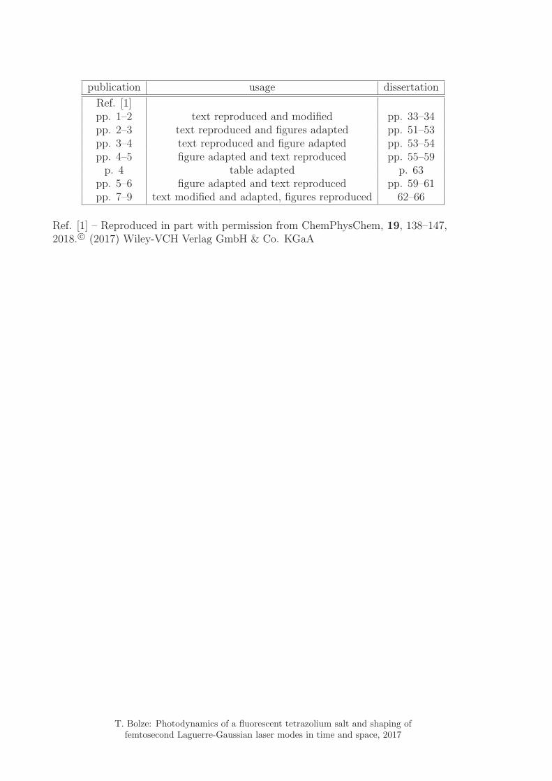
The publication above has partly been used in this thesis. The following table itemizes towhat extent the different sections of the article have been reused at which position in thepresent work. The permission of reproducing this material was given by the publishingcompany holding the copyright, the corresponding document is attached at the end ofthis work. Additionally, the sources of adapted figures are indicated at the end of thecorresponding figure captions.


publication usage dissertation

Ref. [1]pp. 1–2 text reproduced and modified pp. 33–34pp. 2–3 text reproduced and figures adapted pp. 51–53pp. 3–4 text reproduced and figure adapted pp. 53–54pp. 4–5 figure adapted and text reproduced pp. 55–59

p. 4 table adapted p. 63pp. 5–6 figure adapted and text reproduced pp. 59–61pp. 7–9 text modified and adapted, figures reproduced 62–66

Ref. [1] – Reproduced in part with permission from ChemPhysChem, 19, 138–147,2018. c© (2017) Wiley-VCH Verlag GmbH & Co. KGaA


CONTENTS

List of Publications VII

1 Introduction 1

2 Theoretical concepts 52.1 Mathematical description of femtosecond laser pulses . . . . . . . . . . . . 5

2.1.1 Temporal and spectral shape of E(t, ω) . . . . . . . . . . . . . . . . 62.1.2 The influence of dispersion and spectral phase on the temporal shape 92.1.3 Concept of a 4f -pulseshaper . . . . . . . . . . . . . . . . . . . . . . 132.1.4 Spatial properties of electromagnetic waves . . . . . . . . . . . . . . 152.1.5 Nonlinear optical processes . . . . . . . . . . . . . . . . . . . . . . . 21

2.2 Molecules and light . . . . . . . . . . . . . . . . . . . . . . . . . . . . . . . 232.2.1 Electronic structure of molecules . . . . . . . . . . . . . . . . . . . 232.2.2 Transitions in molecules . . . . . . . . . . . . . . . . . . . . . . . . 25

2.3 Time-resolved fluorescence spectroscopy techniques . . . . . . . . . . . . . 272.3.1 Time correlated single photon counting . . . . . . . . . . . . . . . . 292.3.2 Fluorescence upconversion . . . . . . . . . . . . . . . . . . . . . . . 30

3 Experimental Techniques 333.1 Instrumentation for the fluorescence studies . . . . . . . . . . . . . . . . . 33

3.1.1 Sample preparation . . . . . . . . . . . . . . . . . . . . . . . . . . . 333.1.2 Fluorescence quantum yield determination . . . . . . . . . . . . . . 353.1.3 TCSPC device . . . . . . . . . . . . . . . . . . . . . . . . . . . . . 373.1.4 Femtosecond fluorescence upconversion . . . . . . . . . . . . . . . . 38

3.2 Pulse-shaping setup . . . . . . . . . . . . . . . . . . . . . . . . . . . . . . . 403.2.1 The laser system . . . . . . . . . . . . . . . . . . . . . . . . . . . . 403.2.2 LG-mode conversion . . . . . . . . . . . . . . . . . . . . . . . . . . 433.2.3 The 4f -pulseshaper . . . . . . . . . . . . . . . . . . . . . . . . . . . 453.2.4 The combined setup . . . . . . . . . . . . . . . . . . . . . . . . . . 47

4 Fluorescence studies of PTC 514.1 Static absorption and fluorescence spectra . . . . . . . . . . . . . . . . . . 51


X CONTENTS

4.2 Quantum yield measurements . . . . . . . . . . . . . . . . . . . . . . . . . 534.3 Time resolved fluorescence measurements . . . . . . . . . . . . . . . . . . . 55

4.3.1 picosecond-dynamics . . . . . . . . . . . . . . . . . . . . . . . . . . 554.3.2 femtosecond-dynamics . . . . . . . . . . . . . . . . . . . . . . . . . 59

4.4 Interpretation and discussion of the results . . . . . . . . . . . . . . . . . . 62

5 Pulseshaping of fs-Laguerre-Gaussian laser modes 675.1 Setup characterization . . . . . . . . . . . . . . . . . . . . . . . . . . . . . 67

5.1.1 Pulse characterization of the LG and HG Arm . . . . . . . . . . . . 685.1.2 Time integrated LG-HG interference in 1st and 2nd order . . . . . . 705.1.3 Spatially-resolved crosscorrelation of the shaped and unshaped pulses 74

5.2 Temporally shaped LG pulses . . . . . . . . . . . . . . . . . . . . . . . . . 755.3 Time evolution of the spatially resolved LG-HG interference . . . . . . . . 80

5.3.1 Simulation . . . . . . . . . . . . . . . . . . . . . . . . . . . . . . . . 825.3.2 Measurement . . . . . . . . . . . . . . . . . . . . . . . . . . . . . . 85

6 Summary and Outlook 89

List of Abbreviations VII

Biblography XIX

Permissions XXI

Acknowledgements XXIII


CHAPTER 1

INTRODUCTION

Light is as omnipresent in our daily lives as it is essential for it. The perception of light asan electromagnetic wave by James Clerk Maxwell in 1865 was as groundbreaking as it wasingenious at the time and is now considered as one of the greatest intellectual achievementsmankind has ever made. Ever since then the study of the light-matter interactions hasseen a tremendous scientific attention with the goal to unravel the mysteries of life andthe universe.

Among the many quests surrounding electromagnetic radiation is its control and manip-ulation. The prediction of the laser by Einstein and its first experimental realization inthe 1960s gave rise to an array of new techniques and methods for studying light-matterinteractions. For the first time in history a monochromatic light source, that is highlycollimated and intense, was available, although in its first implementations the laser wasdescribed as a solution searching for a problem. An assessment that turned out to bemore than false from today’s point of view. For a review of the laser development seeref. [2]. Soon after the first demonstration of the laser, effort had been made towardssub-nanosecond pulsed lasers, that eventually lead to pulses on the time scale of a couplefemtoseconds (10−15 s). These electromagnetic events are among the shortest man-madeand controllable events and have found their way into several high-tech applications and alot of scientific methods. For example, they offer a great tool to understand the dynamicsof chemical reactions, since those typically take place on time scales down to femtosec-onds. The term femtochemistry describes a junction of chemistry and laser pulses on thistime scale. In 1999 the Nobel Prize in Chemistry was awarded to one of the founders ofthis research field, Ahmed Zewail. Topics in this field range from observing to controllingchemical reactions in real time. The latter was termed quantum control and has given riseto several several schemes that allow the control of quantum mechanical systems [3–7].

The observation of chemical reactions on the other hand has also spawned its own uniquemethods and techniques involving femtosecond laser pulses. Most notably the pump-probescheme [8, 9] is wide-spread and has found its way into many scientific applications. Theadvantage of knowing the exact point in time at which a photo-induced chemical reactionstarts allows for a sampling of the detection with another pulse and thus monitoring thedynamics of the reaction in time. Light induced chemical reactions, that have been stud-


2 1 Introduction

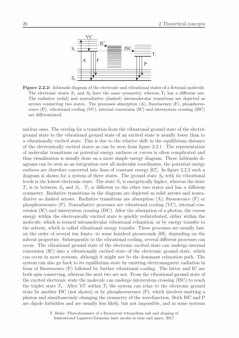
ied extensively by pump-probe schemes are dissociation, isomerization, and intersystemcrossing [7, 10–13], however also intramolecular relaxation processes can be investigatedby these methods. Such dynamics take place after a molecule absorbs energy of some kindand tries to equilibrate the energy within itself or its surroundings. Uptake of energy canlead to several types of dynamics, for example translation, rotation, and vibration. Alsoelectronic excitation is possible, where an electron resting in the ground state of a moleculechanges its potential energy surface, which is followed by another sequence of possible dy-namics. Among those processes is the ability of certain molecules to emit light, whichis called luminescence that can be differentiated into fluorescence and phosphorescence.The latter involves a spin flip in the system and is therefore classically spin forbidden,although spin-orbit coupling especially in larger molecules and atoms might loosen thisrule. Fluorescence does not involve a spin flip and is therefore more common and easierto observe. The dynamics of the light emission of a molecule are strongly related to itsquantum chemical structure, thus may offer insight into the latter. Fluorescence is alsoa way of relaxation for a molecule trying to reach its ground state, as such it is usuallyaccompanied by other intra- and intermolecular relaxation processes. Especially in theliquid phase, where molecules are constantly interacting with the solvent, rich dynamicsappear in the molecule and the solvent trying to equilibrate the energy that is depositedin the system for example though light absorption [14, 15].

The compound class of tetrazolium salts was first described in 1894 by Pechmann andRunge [16]. These molecules are characterized by a low reduction threshold, which makesthem an ideal sensor for monitoring the reductive and oxidative features of their sur-roundings. Since metabolic reactions in the cellular environment often involve changingthe local chemical potential, tetrazolium salts have found their way into many applica-tions surrounding the metabolism of cells. Most notably are techniques in the fields ofagriculture [17, 18], cell biology [19, 20], cancer [21, 22] and other medical research [23, 24],organic chemistry [25, 26], ionic liquids as cations [27, 28], and dosimetry for quantifica-tion of ultraviolet light [29, 30]. One rather unexplored feature of tetrazolium salts istheir emission capability, although it is known that fluorescing specimen exist [31]. Onegoal of this thesis is to elaborate further into the dynamics of this compound by meansof time resolved fluorescence spectroscopy.

Using fluorescent tetrazolium salts in cell biology would for example give access to themethods of fluorescence microscopy, which is a major tool to understand processes inliving cells. Among the most cutting edge fluorescence microscopy methods is stimulatedemission depletion (STED)[32], which was awarded with the Nobel Prize in Chemistryto Stefan Hell in 2014. In 2017 the newest iteration of this technique was reported [33],that is able to determine the coordinates of a molecule with minmal emission fluxes andis termed MINFLUX. The resolution of the STED method was already groundbreaking,as it surpassed the Abbe diffraction limit, however MINFLUX has a reported resolutionof ≈ 1 nm. The concept of both techniques relies on a pump-dump scheme, in whichone laser excites the fluorescent molecules in the sample. A second laser then dumps theexcitation by stimulated emission. The dump-beam has a doughnut-like shape, whereasthe pump-beam is Gaussian in shape. This results in a detectable fluorescence of thesample that only originates from the dark spot in the center of the Laguerre-Gaussian(LG) beam, as doughnut-shaped beams are called.

These LG beams have a unique feature, since they have a helical spatial phase and are


3

therefore carrying an orbital angular momentum (OAM). They have first been described in1992 by Padgett and Allen [34] and a lot of progress has been made in the last two decadesregarding the understanding of their properties and prospective applications. Commercialoptical communication systems use photons for information transfer. To encode as muchinformation as possible into as few photons as possible frequency multiplexing is thecommon technique in optical communication. OAM multiplexing, that can be understoodas a special kind of space-multiplexing, has been demonstrated in free space [35, 36] andfibers [37] to increase the information density much further. Also quantum cryptographyusing entangled pairs of OAM carrying photons is discussed in literature [38–40]. Thelaser systems used in these experiments are either continuous wave or narrow bandwidthinfrared light sources. Although femtosecond pulses with LG beamprofiles have beendemonstrated, not all methods of controlling and measuring fs pulses have been appliedto LG beams yet. To close the gap this work will focus on some of them, namely fstemporal pulse-shaping, frequency conversion, and temporal characterization.This work is ordered as follows: chapter 2 will give an insight into the theoretical conceptsof femtosecond laser pulses, a quantum mechanical description of molecules and their tran-sitions, and time-resolved fluorescence spectroscopy techniques used in this work. Chap-ter 3 gives a detailed overview of the instruments and methods used for the experiments.Chapter 4 will give an overview of the studies performed on the fluorescence dynamics ofPTC in alcoholic solutions. First, steady-state absorption and emission spectroscopy willbe employed to get information on the general electronic structure of the molecule andits fluorescence quantum yield in several alcoholic solvents. Time-resolved experimentswith varying excitation wavelengths using time correlated single photon counting (TC-SPC) and fs-fluorescence upconversion will be shown, that consistently demonstrate thatone dominant process is responsible for the majority of the PTC fluorescence. Dynamicsthat depend on the alcoholic solvent used will be shown and discussed, in order to gaina deeper understanding of the intramolecular processes. Moreover solvent related relax-ation dynamics will be disclosed with respect to the ultrafast part of the fluorescence. Theaccumulated observations will then be discussed and joined into a photoreaction schemeof PTC.In chapter 5 the results of the experiments involving fs-LG pulses will be presented. Aftera detailed characterization of the mode conversion and related parts of the beam path itwill be demonstrated that LG pulses can be generated from temporally shaped fs pulsesand characterized by the same means as Hermite-Gaussian (HG) pulses. The last partof this chapter will deal with the temporal evolution of the LG-HG interference of twofs pulses. Its behavior in time will be calculated using space-time dependent fields and amethod will be explored that involves frequency conversion to visualize and measure thistime evolution. An experimental approach will be done to measure the predictions anddiscuss them in the context of the simulations.The work will be summarized in chapter 6, a discussion will be given, and future experi-ments that could extend the findings of this work will be outlined.


4 1 Introduction


CHAPTER 2

THEORETICAL CONCEPTS

This chapter will provide an overview of the theoretical concepts of the experimentspresented in this thesis, which is divided in two parts. The first focuses on the investigationof fluorescence dynamics of molecules in different solvents. Since these processes occuron ultrashort time scales, techniques must be used that have access to these types ofshort-time events. This feat is accomplished by the use of laser pulses, which are shorterthan the dynamics that are investigated. These light pulses are also highly controllable interms of wavelength and timing, which makes them the ideal tool to start photoinduceddynamics and to monitor them as well. The second part will deal with manipulating thefield of such a laser pulse in terms of its exact temporal and spatial shape. Therefore, adeep understanding of laser pulses as a prerequisite to all presented experiments is needed,which is given in section 2.1 of this chapter. It is followed by a section dealing with thequantum mechanical description of molecular systems in 2.2. In the end two time resolvedspectroscopy techniques, that are used for the experiments in this thesis, will be presentedin section 2.3.

2.1 Mathematical description of femtosecond laser

pulses

In 1861 James Clerk Maxwell published his work on electromagnetism[41], wherein for-

mulas that describe the interactions of electric ~E and magnetic ~B fields can be found.Based on that he published his ”Electromagnetic Theory of Light” four years later [42].Light as an electromagnetic wave can be can be described by the Maxwell equations intheir Heavyside form:[43]

~∇ · ~E =ρ

ǫ0(2.1.1)

~∇ · ~B = 0 (2.1.2)


6 2 Theoretical concepts

~∇× ~E = −∂ ~B

∂t(2.1.3)

~∇× ~B = µ0~J + µ0ǫ0 ·

∂ ~E

∂t(2.1.4)

with the charge density ρ, the permittivity of free space ǫ0, the permeability of freespace µ0 and the current density ~J . These equations describe light as well, due to theirelectromagnetic nature, as Maxwell later deduced. Since light or electromagnetic radiationis omnipresent, its nature and interaction with matter is of great importance to understandphenomena and processes in our world. The invention of the laser (light amplification bystimulated emission of radiation) in the early 60s as a tool for these investigations wasgroundbreaking. For the first time in history an intense light source with coherent andhighly collimated emission was available. Nowadays, lasers are widely used in almostevery major industrial branch. On top of continuous emission also pulsed lasers havebeen constructed and have established themselves as a powerful tool for spectroscopicinvestigations of atomic and molecular systems.This section will deal with the mathematical formulation of light pulses. First, a generaldescription of the temporal and spectral structure of a pulse and its interconnection willbe given in section 2.1.1. Then the effect of natural dispersion on the spectral phaseand thus the temporal shape of the pulse will be discussed in section 2.1.2. Thereaftera concept of arbitrary alteration of the spectral phase will be introduced in section 2.1.3with the principles of a 4f -Pulseshaper. Section 2.1.4 will deal with the spatial propertiesof plane and non-planar waves. Discussion of nonlinear optical processes relevant to thiswork will top this section of in 2.1.5.

2.1.1 Temporal and spectral shape of E(t, ω)

Inserting ~∇× ~B from equation 2.1.4 in the curl of ~∇× ~E in equation 2.1.3 and using thevector identity ∇×∇× E = ∇(∇ · E) −∇2E leads to the wave equation in free space:

∇2E = µ0ǫ0∂2E

∂t2. (2.1.5)

Assuming a plane wave, equation 2.1.5 simplifies to the plane wave equation

∂2E

∂z2= µ0ǫ0

∂2E

∂t2(2.1.6)

where z is the direction of propagation. The sinusoidal solution to equation 2.1.6 for laserpulses takes the form:

E(z, t) = A(t) · cos(ω0t + φ0 + φ(t)) (2.1.7)

where A(t) denotes time-dependent amplitude, ω0 the central angular frequency, φ0 theconstant phase and φ(t) the time-dependent phase. Both phases have no impact on theenvelope of the pulse, since its amplitude part is separated from the oscillating part,however, especially the time-dependent phase may change the frequency of the oscillationover the duration (e.g. the course) of the pulse. Therefore, the instantaneous frequencyω(t) is defined as


2.1 Mathematical description of femtosecond laser pulses 7

ω(t) =d

dt· (ω0t + φ0 + φ(t)) = ω0 +

dφ(t)

dt. (2.1.8)

An equivalent form of equation 2.1.7 can also be written as

E(z, t) = Re[

A(t)eiω0teiφ0eiφ(t)]

(2.1.9)

where Re denotes the real part. Here the separation of amplitude, oscillatory part andphase becomes apparent as well.Since the superposition principle holds, a laser pulse that is fixed in space can be repre-sented by a series of monochromatic waves that are fixed in space as well. This so-calledFourier decomposition is described by the Fourier transform

E(t) =1

2π

∞∫

−∞

E(ω)eiωtdω (2.1.10)

and the inverse Fourier transform

E(ω) =

∞∫

∞

E(t)e−iωtdt. (2.1.11)

This interconnection of time space and frequency space is known from acoustics[44, 45].In optics the same principles holds, a short event has to have a broad spectrum, whereas anarrow spectrum corresponds to a near constant signal in time. Laser pulses can actuallybecome so short (sub 5 fs) that their spectrum spans the whole visible region of theelectromagnetic spectrum.Analogue to equation 2.1.9 the spectral electric field can be separated into an amplitudeand phase part. In its nature as the Fourier transform of the real valued temporal electricfield, which is not necessarily symmetric with respect to time, the spectral electric fieldin general is complex and takes the form

E(ω) =√

I(ω)e−iφ(ω), (2.1.12)

where I(ω) is the spectral intensity, which is proportional to the power spectral densitythat can be measured with a spectrometer, and φ(ω) is the spectral phase. Analogue tothe instantaneous frequency, which describes the instance at which a certain frequency ispresent in time, a measure of the time delay for a specific frequency component can bederived from φ(ω). This parameter is called group delay

Tg(ω) =dφ(ω)

dω. (2.1.13)

For any spectral phase φ(ω) independent of the frequency ω the spectral and temporalamplitudes satisfy the uncertainty relation

∆t∆ω ≥ K (2.1.14)

where the constant K depends on the shape of the spectrum. For Gaussian spectra,which will be discussed exclusively in this thesis, the constant becomes K = 0.441. This



2 0. 2 2. 2 4. 2 6. 2 8.frequency (rad/fs)

-10

0

10

f(w

) (r

ad)

-100

0

100

200

T ( g

w)

(fs)

(a)

-40 -20 0 20 40time (fs)

0

5

10

f(t

) (r

ad)

2 2.

2 4.

2 6.

w(t

) (r

ad/f

s)

(b)

Figure 2.1.1: A bandwidth limited pulse with a central wavelength of 800 nm and a temporalFWHM of 10 fs. Spectral intensity I(ω), spectral phase φ(ω) and group delay Tg(ω) areshown in (a). Temporal Intensity I(t), temporal phase φ(t) and instantaneous frequency ω(t)are displayed in (b).

relation is known as the time-bandwidth product. A pulse that satisfies the equality iscalled bandwidth limited or Fourier-transform limited. An example of such a pulse isdisplayed in figure 2.1.1 for a central wavelength of 800 nm and a temporal full width athalf maximum (FWHM) of 10 fs. The spectral intensity I(ω) along with the spectral phaseφ(ω) and the group delay Tg(ω) is illustrated in the left panel. Note that the spectralphase (and group delay) is zero over the whole spectral range of the pulse, which meansthat the pulse is bandwidth limited. In the right panel, the temporal intensity I(t) isdepicted along with the temporal phase φ(t) and the instantaneous frequency ω(t). Thephase is again zero over the whole duration of the pulse and ω(t) is constant at 2.35 rad

fs,

which is the central angular frequency. Any non-zero spectral phase can be expanded ina Taylor series for quantification. This series expands the phase into

φ(ω) =∞∑

n=0

φn(ω0)

n!· (ω − ω0)

2

with

φn(ω0) =dnφ(ω)

dωn

∣

∣

∣

∣

ω=ω0

.

Aborting the series after n = 3 yields:

φ(ω) = φ(ω0) + φ′(ω0)(ω − ω0) +1

2φ′′(ω0)(ω − ω0)

2 +1

6φ′′′(ω0)(ω − ω0)

3. (2.1.15)

The effect of every polynomial of this series on the pulse shape will be discussed in thenext subsection. Any nonlinear term applied to the spectral phase results in the inequalityof equation 2.1.14 and thus broadens the pulse.



-10 -5 0 5 10-1 0.

-0 5.

0 0.

0 5.

1 0.E

(t)

a u

.(

.)

t fs( )

(a)

-1 0.

-0 5.

0 0.

0 5.

1 0.

E(t

)a.

u.

()

-10 -5 0 5 10t fs( )

(b)

Figure 2.1.2: Temporal electric field (black) and envelope (red) of a pulse with a centralwavelength of 800 nm and a temporal FWHM of 5 fs. If the spectral phase φ(ω) = 0 themaximum of the field and envelope coincide, leading to a cosine pulse (a). For a spectralphase of φ(ω) = π

2 the field is zero at the maximum of the envelope, leading to a sine pulse(b).

2.1.2 The influence of dispersion and spectral phase on the tem-poral shape

The simplest polynomial spectral phase is that of a constant, which is represented by thefirst term in equation 2.1.15. This term is often called b0 and has no influence on theamplitude part of the temporal electric field but on the oscillatory part from equation2.1.7. More precisely b0 is the phase between the envelope and the oscillation, thus onlybecomes relevant for pulses that are consisting of only a few optical cycles[46, 47]. Infigure 2.1.2 the oscillatory (red) and the amplitude (black) part of a pulse with a centralwavelength of 800 nm and a FWHM of 5 fs are shown for a constant spectral phase ofφ(ω) = 0 (left) and φ(ω) = π

2(right). For a phase of zero, a maximum of the oscillation

and the maximum of the envelope coincide at time t = 0 fs. This is called a cosine pulse.In case of φ(ω) = π

2the oscillation is shifted a quarter of an optical cycle, which leaves

the electric field at time zero E(0) = 0, thus generating a sine pulse. The implicationof this is a slightly reduced maximum electric field strength, which can become relevantfor highly nonlinear processes with few-cycle pulses[48, 49]. In the scope of this thesis,however, no such pulses are used.

The linear polynomial term of the spectral phase (referred to as b1) does not change theoscillatory part of the electric field but the maximum of its envelope and thus shiftingthe pulse in time. Thereby, the pulse shape is not altered. In figure 2.1.3 the spectral(left) and temporal (right) intensities of an 800 nm pulse with a temporal FWHM of 10 fsand a linear spectral phase of b1 = 20 fs are shown along with the respective phases φ(ω)and φ(t), the group delay Tg(ω), and the instantaneous frequency ω(t). By applying alinear spectral phase, a constant group delay is introduced according to equation 2.1.13,which corresponds to a shift in the time domain. The temporal phase and instantaneousfrequency, however, are not changed. The direction in which the pulse is temporallyshifted is determined by the sign of b1, the reference is the time zero of a pulse without aspectral phase.

The quadratic spectral phase term is referred to as ‘linear chirp’ and denoted as b2. Ac-



-10

0

10

f(w

) (r

ad)

(a)

2 0. 2 2. 2 4. 2 6. 2 8.frequency (rad/fs)

-100

0

100

200

T ( g

w)

(fs)

-40 -20 0 20 40time (fs)

0

5

10

f(t

) (r

ad)

2 2.

2 4.

2 6.

w(t

) (r

ad/f

s)

(b)

Figure 2.1.3: A pulse with a central wavelength of 800 nm, a temporal FWHM of 10 fs and alinear spectral phase term b1 = 20 fs. Spectral intensity I(ω), spectral phase φ(ω) and groupdelay Tg(ω) are shown in (a). Temporal Intensity I(t), temporal phase φ(t) and instantaneousfrequency ω(t) are displayed in (b).

cording to equations 2.1.8 and 2.1.13 it induces a linear change of the instantaneousfrequency and the group delay, respectively. This entails that the different spectral com-ponents get ordered in time by increasing or decreasing frequency for positive or negativesigns of b2, respectively. A positive sign is referred to as an up-chirp and a negative as adown-chirp. In figure 2.1.4 the spectral (left) and temporal (right) intensities of a pulsewith 800 nm central wavelength and a temporal FWHM of 10 fs with a quadratic spectralphase of b2 = 200 fs2 is shown. The integral of the intensity over time, which is equivalentto the pulse energy, of the chirped pulse in figure 2.1.4 is the same as for the shifted pulsein figure 2.1.3. But due to the temporal broadening in case of a quadratic spectral phasethe peak intensity decreases, thus any process dependent on the intensity (but not theenergy) is sensitive to a chirp in the pulse. However, any pulse only becomes stretchedout in time due to a quadratic spectral phase. If Gaussian spectra are considered, thepulse length ∆tout of an input pulse ∆tin after applying a quadratic spectral phase of φ′′

can be estimated via[47, 50]

∆tout =

√

∆t2in +

(

4ln2φ′′

∆tin

)2

. (2.1.16)

The cubic spectral phase term (also called Third Order Dispersion) gives rise to aquadratic group delay. This leads to a fragmentation of the pulse. The central frequency(around which the phase is applied) carries most of the spectral intensity and is almostnot influenced by the phase, since a cubic function is in first approximation zero aroundω0. This results in a big sub-pulse around time zero, which is mostly composed of thecentral frequency components. However, around the carrier frequency all electromagneticwaves are dispersed in a way that two components with the same spectral separation fromthe central frequency, but in opposite directions, have the same delay. The instantaneousfrequency remains constant, since the mean of all occurring waves at any time is equal tothe central frequency. However, at any time two electromagnetic waves with different fre-quencies overlap and may interfere constructively or destructively. For some delay timesthis results in an annihilation and thus, a knot in the intensity profile and a formationof pulse fragments with different spectral composition. The temporal phase in this case



-10

0

10f

(w)

(rad

)(a)

2 0. 2 2. 2 4. 2 6. 2 8.frequency (rad/fs)

-100

0

100

200

T ( g

w)

(fs)

-40 -20 0 20 40time (fs)

0

5

10

f(t

) (r

ad)

2 2.

2 4.

2 6.

w(t

) (r

ad/f

s)

(b)

Figure 2.1.4: A pulse with a central wavelength of 800 nm, a temporal FWHM of 10 fs anda quadratic spectral phase term b2 = 200 fs2. Spectral intensity I(ω), spectral phase φ(ω)and group delay Tg(ω) are shown in (a). Temporal Intensity I(t), temporal phase φ(t) andinstantaneous frequency ω(t) are displayed in (b).

jumps from 0 and π and back between the sub-pulses. This is illustrated in figure 2.1.5,where the spectral intensity, phase, and group delay is depicted on the left and the tem-poral intensity, phase, and instantaneous frequency is depicted on the right for a pulsewith a central wavelength of 800 nm, a temporal FWHM of 10 fs and a cubic spectralphase of b3 = 1000 fs3. Phase components of third order also occur naturally in opticalmedia, however, they are usually in the same order of magnitude than second order dis-persion [47] and are therefore less relevant, due to their cubic dependence (ω−ω0)

3. Thenatural dispersion may introduce complex amplitude and phase modulation in the timeand frequency domain for ultrashort laser pulses. In general, the perturbation introducedvia dispersion can be described by a temporal M(t) and spectral M(ω) transfer function.Both functions represent a Fourier pair.

M(t) =1

2π

+∞∫

−∞

M(ω)eiωtdω ⇐⇒ M(ω) =

+∞∫

−∞

M(t)e−iωtdt

If a pulse propagates through an optical element the electric field Ein(t) of the pulse getsconvoluted with the transfer function M(t) according to:

Eout(t) = Ein(t) ⊗M(t) =

+∞∫

−∞

M(t− t′)E+in(t′)dt′

and results in the electric field Eout(t) after passing through the element. The convolutiontheorem states that a convolution in one Fourier domain equals a multiplication of theFourier pairs in the other domain. In the present case this leads to the much easierexpression

Eout(ω) = Ein(ω) ·M(ω), (2.1.17)

where the incoming spectral electric field Ein(ω) gets multiplied with the spectral transferfunction yielding the outgoing spectral electric field. The spectral transfer function canbe written analogously to the spectral electric field of the pulse as



-10

0

10

f(w

) (r

ad)

(a)

2 0. 2 2. 2 4. 2 6. 2 8.frequency (rad/fs)

-100

0

100

200

T ( g

w)

(fs)

-40 -20 0 20 40time (fs)

0

5

10

f(t

) (r

ad)

2 2.

2 4.

2 6.

w(t

) (r

ad/f

s)

(b)

Figure 2.1.5: A pulse with a central wavelength of 800 nm, a temporal FWHM of 10 fs anda cubic spectral phase term b3 = 1000 fs3. Spectral intensity I(ω), spectral phase φ(ω)and group delay Tg(ω) are shown in (a). Temporal Intensity I(t), temporal phase φ(t) andinstantaneous frequency ω(t) are displayed in (b).

M(ω) = AM(ω)e−iφM (ω), (2.1.18)

where AM(ω) is the amplitude modulation, which is equivalent to the frequency dependentabsorption of the element, and φM(ω) is the phase modulation of the element[47, 51].Inserting equation 2.1.18 into 2.1.17 vividly illustrates that the modulation phase getsadded to the inherent phase of the pulse and therefore alters the pulse even in the absenceof any absorption. Thus, the above-described decomposition of the spectral phase intopolynomials of different orders is also useful for the natural dispersion of optical elements.A linear spectral phase is introduced by any optical element that involves the change ofthe refractive index. Since the speed of light c in a medium is connected to the speed oflight in vacuum c0 via the refractive index by

c =c0n

any change in the refractive index leads to a delay due to the lower velocity in the mediumrelative to a propagation where there is no medium. This delay can then be described bya linear spectral phase component b1. The refractive index is in general also a functionof frequency (or wavelength λ), therefore the speed of light in a medium is dependent onthe frequency of the wave. If all the electromagnetic waves that make up a pulse enteran element with frequency dependent refractive index, every wave exits the medium witha different delay. Thus, an ordering of the frequencies is created, which can be describedby a quadratic phase term b2. Cubic phases may also be introduced by dispersion ofoptical elements, but are less relevant as discussed above. Higher order terms can oftenbe neglected for linear optical media. The wavelength dependence of the refractive indexof a given optical medium is usually a complex function. For wavelength that are notclose to an absorption resonance of the medium, the refractive index function can beapproximated by the empirical Sellmeier equation

n2(λ) = 1 +B1λ

2

λ2 − C1

+B2λ

2

λ2 − C2

+B3λ

2

λ2 − C3

(2.1.19)

with Bi and Ci being material constants. These coefficients are known and tabulated



400 600 800 1000

2 4688.

2 4692.

2 4696.

refr

activ

e in

dex

n

wavelength (nm)

Figure 2.1.6: Approximation of the dispersion of the refractive index n(λ) for N-SF66 glassusing the Sellmeier equation 2.1.19 for the visible and near infrared region.

by optical glass supplying companies (e.g. SCHOTT AG). For example for the glass N-SF66 the constants are: B1 = 2.0245976, B2 = 0.470187196, B3 = 2.59970433, C1 =0.0147053225, C2 = 0.0692998276 and C3 = 161.817601 [52]. An empirical approximationof the dispersion of the refractive index for N-SF66 can thus be made and is shown infigure 2.1.6 for the visible and near infrared region.

2.1.3 Concept of a 4f-pulseshaper

The effect of dispersion is usually an unwanted one occurring in all transparent opticalmedia. However, the dispersion of a pulse may be compensated for by applying the samedispersion with a negative sign. Normal transparent media in the visible spectral regimeare not suited for this, since the sign of the dispersion they introduce is always positive,unlike for the IR regime, where negative dispersion is possible [53]. But with diffractiveelements such as prisms or gratings, it possible to disperse the pulse spectrally in space andthen manipulate each frequency independently. Therefore an arrangement of two prismsor gratings and a mirror may be sufficient to compensate the natural positive dispersionby introducing a variable negative dispersion. These devices are called (prism or grating)compressor and are used routinely in mode-locked laser systems for dispersion control andin amplifier systems to enable chirped pulse amplification. An approach to imprint morearbitrary phases on pulses and thus, enable access to the field of pulse shaping, is theuse of a zero dispersion compressor (ZDC) and a phase mask [54]. A ZDC is composedof two gratings or prisms and two cylindrical lenses or mirrors. The input pulse getsdiffracted by the first grating (or prism). The first diffraction order is then collimatedby a cylindrical lens (or mirror), which has its focus where the beam is diffracted on thegrating. At a distance of one focal length in the direction of light propagation is the socalled Fourier-plane. This is where each spectral component is projected into a sharpline. Putting a CCD detector here would yield the spectrum of the pulse. The ZDC iscompleted by a mirrored arrangement of a lens/mirror and a grating/prism, which has itsFourier-plane at the exact same location as the first setup. This device disperses the pulsespectrally, collimates it and then recombines the spectral components into a pulse again,without introducing any dispersion. However, it is easy to insert any phase or amplitudemask into the Fourier-plane of this device and thus, altering the spectral amplitude or



f f ff

LC-SLM

Fourier-plane

Figure 2.1.7: Basic layout of a 4f -pulseshaper based on a zero dispersion compressor (ZDC)consisting of two gratings and two cylindrical lenses. The distance between the point ofspatial dispersion and recombining of the pulse is four times the focal length as indicated. Inthe Fourier-plane a spatial light modulator (SLM) is placed to exert control over the spectralphase or amplitude of the pulse.

phase of the pulse. It is known from the previous section that such manipulation leads tocontrol over the temporal profile as well.

It is evident that the shaping capabilities of this setup is highly dependent on the qualityof the phase mask. For this purpose liquid crystal spatial light modulators (LC-SLM) arewidely used [55–57]. These electronic devices are inserted into the Fourier-plane of thedescribed ZDC and can be controlled via a computer. The geometry of this setup suggeststhe name of this device as a 4f -pulseshaper, since it expands over a distance, which isjust over four times the focal length of the used lenses/mirrors, to shape the spectralproperties of the pulse. The whole setup is illustrated in figure 2.1.7. The LS-SLM isan electro-optical element consisting of two glass substrates with programmable pixels inbetween. These pixels are composed of two transparent electrodes made of indium tinoxide over which a voltage can be applied, as is depicted in figure 2.1.8a. In betweenthese electrodes a solution of a nematic liquid crystals of rod-like molecules is placed. Inabsence of any voltage these rods are prealigned (see figure 2.1.8b) and therefore, the wholepixel is birefringent in nature because of the anisotropy of the electric dipole moments.Applying a voltage to the electrodes leads to a new alignment of the dipole moments ofthe liquid crystal molecules along the field lines (see figure 2.1.8c). This rotation takesplace in one plane and therefore may change the refractive index of the pixel for anelectromagnetic wave that is polarized in this plane. This can be done for every spectralcomponent of the pulse separately and thus introduces a different group delay for everycomponent, thereby changing the spectral phase of the pulse. This procedure is calledphase shaping and alters the exponential term in equation 2.1.18. It is also possible tomanipulate the amplitude of each spectral component, which corresponds to control overthe first term in equation 2.1.18. This is achieved by placing a polarizer in front of theLC-SLM and a second one in crossed position behind the electro-optic element. Theplane of alignment for the liquid crystals has to be 45◦ with respect to both axes of thepolarizers. Thus the linear polarized electric field that enters a pixel can be written as twoseparate linear components that are polarized perpendicularly to each other. One of thepolarization components is parallel to the plane of the liquid crystals and therefore maybe manipulated. This results in a change of the polarization state of the overall electricfield that exits the pixel. The second polarizer then absorbs the field either partially orcompletely and thereby alters the amplitude of that spectral component. This procedure



zxy

liquid crystal

ITO electrodes

glass substrate(a)z

yx

(b)

substrate ITOLC molecule

zy

x(c)

Figure 2.1.8: Basic layout of the pixels in an LC-SLM. (a) Front view: the pixelated indiumtin oxide (ITO) electrodes are coated on the insides of the glass substrates and the liquidcrystal solution is sealed inside. The light propagates in z-direction. (b) Top view into asingle pixel with no voltage applied. All liquid crystals are oriented in y-direction. Uponapplying a voltage the molecules rotate to face into the z-direction (c), thereby changing therefractive index for an electromagnetic wave with its polarization in the y-plane.

is done for every spectral component of the pulse and thus, amplitude shaping of thespectrum of a pulse is possible. By leaving the second polarizer out of the setup the sameapproach can be used to shape the polarization state of each spectral component[58, 59].This whole technique can be expanded by using multilayer LC-SLMs [60], which enablethe simultaneous control of two [61, 62] or even all three [63] of the mentioned properties.

2.1.4 Spatial properties of electromagnetic waves

The properties of electromagnetic waves discussed so far are solely time (or frequency)dependent. However, for the description of laser beams with their spatial and directionalproperties this is not sufficient. Therefore, the electric field in the wave equation 2.1.5 forbeams is in general a function of the spatial variable r =

√

x2 + y2 + z2. Furthermorethe solution of 2.1.5 can also be complex, as already indicated by equation 2.1.9. Thus,complex valued solutions of the wave equation may take the form:

E(r, t) = E(r)A(t)eiω0teiφ0eiφ(t). (2.1.20)

Note that the spatial and temporal properties of the wave are separated here. Solutionsfor the temporal part of equation 2.1.20 have been discussed in section 2.1.1. In this caseit was assumed that E(r) = 1, hence equation 2.1.20 is a more generalized ansatz. Usingthis equation in the wave equation the Helmholtz equation for E(r) is obtained: [43]

∇2E(r) + k2E(r) = 0 (2.1.21)

with

k2 =ω2

c2.

One solution of the Helmholtz equation is



E(r) = E0eikr,where k is the absolute value of the wave vector that is assumed to always point in thez-direction and E0 is a constant. Such a solution is called a plane wave and the electricfield has the same amplitude at any point in a plane perpendicular to the z-direction.Thus, the field expands infinitely in the xy-plane. This does not describe regular laserbeams, since they are not infinitely spread out. Another solution of 2.1.21 is

E(r) =C

reikr

where C is a constant. This field has the same amplitude on a sphere centered at x = 0,y = 0, z = 0 and is therefore called a spherical wave. Considering propagation in z-direction, the z coordinate may be replaced with the curvature radius R of the planewave. Thus the spatial variable r changes to

r =√

x2 + y2 + R2.

However, spherical waves do neither describe laser beams, since they are propagating inall spatial directions at the same time and their intensity decreases by the inverse squarelaw with respect to the point source, from which they originate. Beam-like solutions ofequation 2.1.21 take the form

E(r) = E0(r)eikz. (2.1.22)

Assuming that E0(r) and∂E(r)

∂zonly slowly changes with z leads to the paraxial approxi-

mation of the Helmholtz equation

∇2TE0(r) + 2ik

∂E0∂z

= 0 (2.1.23)

which every beam-like electromagnetic wave has to satisfy [43]. In the most prominentform the solution to this equation takes the form of a Gaussian in the plane perpendicularto the propagation direction. It can be written as

E0(x, y, z) = Aeikx2+y2

2q(z) eip(z), (2.1.24)

where A is a constant, q is a complex beam parameter that describes the size of thebeamprofile in the xy-plane and p is a spatial phase parameter. Since both q and p areallowed to vary with z the beam diameter and phase within the spatial distribution maychange upon propagation, respectively. Equation 2.1.24 is a solution to equation 2.1.23 ifq(z) and p(z) meet certain requirements [43] that are

1

q(z)=

1

R(z)+

iλ

πw2(z)

and

p(z) = iln

(

q0 + z

q0

)



xz

y

optical axis

w0

√ ∙w2 0

z0

z = 0

wavefronts

x

w(z)

Figure 2.1.9: Gaussian laserbeam that propagates in space along z. The parameters char-acterizing the beam are the beam waist w0 and the Rayleigh range z0. Also displayed isthe divergence angle ξ, the curvature of the wavefronts and change of the curvature uponpropagating through z = 0.

where R(z) is the radius of curvature of the waves at z, w(z) is the spot size, that isthe radius at which the intensity of the Gaussian distribution has decreased to a factor1/e2 of its peak intensity [43] and q0 = q(0). By allowing q(z) and p(z) to be complex,it is possible to describe the complex spatial electric field by real parameters, which isconvenient for describing laser radiation. Following this approach

R(z) = z +z20z

and

w(z) = w0

√

1 +z2

z20

can be obtained. Where z0 is defined by

z0 =πw2

0

λ

and is known as the Rayleigh range, and w0 is the minimal sport size called beam waistalong the direction of propagation. It is by definition located at z = 0. The Rayleighrange is the point in z-direction at which the beam waist has grown to

√2w0 and thus,

describes how collimated the beam is. Following the above assumptions the last term inequation 2.1.24 can be rewritten as

eip(z) =1

1 + izz0

=1

√

1 + z2

z20

e−iϕ(z) =w0

w(z)e−iϕ(z)

with

ϕ(z) = arctanz

z0.



ϕ(z) is called the Gouy phase and it describes the direction in which the wave front iscurved upon propagation along z. In figure 2.1.9 the beam parameters for a Gaussianbeam traveling along z and having a beam waist at z = 0 are visualized. The divergenceangle ξ is also depicted. For z >> z0 it can be assumed that the spot size grows linearlywith z and thus, ξ ≈ w0

z0. Note that figure 2.1.9 also displays the wavefronts of the

electromagnetic wave along z and that the direction of curvature is the same for −∞ <z < 0, but flips at z = 0 to be opposite for 0 < z < ∞. The behavior is described bythe Gouy phase. This also implies that only at z = 0 the wavefronts are truly planarand outside the beam waist the wavefronts are curved like those of a spherical wave. Forz → ∞ the radius of curvature of the wave goes to infinity and therefore the Gaussianbeam can be approximated as a plane wave for large z.Bringing all the above definitions together to formulate the spatial field of a Gaussianlaserbeam leads to:

E(x, y, z) = Aw0

w(z)eik

x2+y2

2R(z) e−x2+y2

w2(z) eikze−iϕ(z). (2.1.25)

Higher-order Hermite-Gaussian laser beams

Equation 2.1.25 is however, only the simplest solution to the Helmholtz equation 2.1.21.Equation 2.1.24 can be modified to obtain a more generalized ansatz [43] in the form of

E0(x, y, z) = A · g(

x

w(z)

)

h

(

y

w(z)

)

eiP (z)eikx2+y2

2q(z) . (2.1.26)

The functions g and h scale with the spot size and determine the beam profile in thexy-plane perpendicular to the direction of propagation. Since g and h are functions ofindependent variables, a separation ansatz can be used to solve the differential equa-tions associated with solving the wave equation. However, this whole procedure is ratherlengthly [43] and therefore the solutions will only be discussed qualitatively here. Thedifferential equations obtained for g and h are independent of each other, but resemble theproblem of the harmonic oscillator from quantum mechanics. Thus, it is not surprisingthat the solutions g and h are in fact a perpendicular basis set formed by the Hermitepolynomials [64, 65]

g

(

x

w(z)

)

= Hm

(√2

x

w(z)

)

h

(

y

w(z)

)

= Hn

(√2

y

w(z)

)

with m and n being integer numbers describing the order of the polynomial. The phaseparameter P (z) in equation 2.1.26 reduces such that

eiP (z) =w0

w(z)e−i(m+n+1)ϕ(z).

Putting the solutions together yields the generalized Hermite-Gaussian field equation forlaser beams:

Emn(x, y, z) = Aw0

w(z)Hm

(√2

x

w(z)

)

Hn

(√2

y

w(z)

)

eikx2+y2

2R(z) e−x2+y2

w2(z) eikze−i(m+n+1)ϕ(z).

(2.1.27)



HG00 HG01 HG02

HG10 HG11 HG12

HG20 HG21 HG22

Figure 2.1.10: Intensity patterns of Hermite-Gaussian leaser modes according to equation2.1.27 for mode indices of m = 0, 1, 2 and n = 0, 1, 2.

For m = 0 and n = 0 it is apparent that equation 2.1.27 reduces to equation 2.1.25since the zeroth Hermite polynomial is a constant. Therefore, the simplest solutions ofthe Helmholtz equation is part of the more generalized set of solutions obtained here.In figure 2.1.10 the intensity of the simplest Hermite-Gaussian (HG) modes are depictedfor m = 0, 1, 2 and n = 0, 1, 2. For increasing m or n an increasing number of intensitynodes appear within the beam profile. The nodes are oriented horizontally and vertically,also note their regular distribution. Most lasers produce exclusively the lowest ordermode HG00, however, this can be changed by introducing a slight disturbance withinthe cavity. If done correctly this disturbance lowers the gain for the HG00-mode andthe cavity prefers oscillation in a higher-order mode. This principle can also be used tosuppress any higher-order mode.

Laguerre-Gaussian laser beams

From figure 2.1.10 it can be seen that the HGmn modes show a rectangular symmetry.This is due to the Cartesian notation x and y in the plane perpendicular to the directionof propagation. By transforming the coordinates into the polar representation in r and θ,where r is now the distance from the beam propagation axis, a different set of solutionscan be obtained for the Helmholtz equation in polar coordinates. This set of solutionstakes the form [34]

Epl(r, θ, z) = Aw0

w(z)

(

r√

2

w(z)

)l

Llp

(

2r2

w2(z)

)

eikr2

2R(z) e− r2

w2(z) eikze−i(2p+|l|+1)ϕ(z)e−ilθ

(2.1.28)

with Llp being the associated Laguerre polynomials defined by [64, 65]



LG00 LG01 LG02

LG10 LG11 LG12

LG20 LG21 LG22

(a) (b)

Figure 2.1.11: Intensity patterns of Laguerre-Gaussian laser modes according to equation2.1.28 for mode indices of p = 0, 1, 2 and l = 0, 1, 2 (a) and the corresponding spatial phaseson a scale from −π to π (b).

Llp(x) = x−l

(

ddx

− 1)p

p!xp+l.

The second fracture in equation 2.1.28 results in radial nodes in the intensity pattern, whileLlp determines the intensity distribution around the nodes. The last exponential term e−ilθ

in equation 2.1.28 leads to an azimuthal phase going on a circle around the beam axis.For any l 6= 0 this results in the existence of a phase singularity on the beam axis since allazimuthal phases from 0 to 2π are present. This produces an additional intensity node onthe beam axis. This spatial phase corresponds to a orbital angular momentum (OAM) ofthe beam, which is not to be confused with the spin angular momentum of photons, whichis associated with the polarization state. A photon can carry a spin and an orbital angularmomentum, the total angular momentum is the sum of both. The intensity pattern ofthe first Laguerre-Gaussian LGpl laser modes for p = 0, 1, 2 and l = 0, 1, 2 are illustratedin figure 2.1.11a. For p = 0 and l = 0 equation 2.1.28 again reduces to equation 2.1.25and thus the lowest order mode in this basis set is the simple Gaussian laser mode again.The azimuthal phases of the modes are displayed in figure 2.1.11b on a scale from −π toπ. One unique property of the LGpl mode set is that the mode indices l can also becomenegative integer numbers. This changes the handedness of the azimuthal phase, analogueto left- and right-handed polarization states. An interesting side effect of this is thatthe total angular momentum of a photon can be zero although the photon is circularlypolarized, when the orbital angular momentum of the photon has the same magnitudebut the opposite sign.



2.1.5 Nonlinear optical processes

To describe the light matter interaction, Ampere’s law in the Maxwell equations has tobe generalized from its free space form to contain the properties of the medium [50]. Tothat end the electric flux density D = ǫ0E+P is introduced. The modified equation takesthe form:

∇× B = µ0J + µ0ǫ0 ·∂E

∂t+

∂P

∂t

with the polarization P of the medium

P = χeǫ0E

that can be understood as the result of the interaction between field and medium. Theparameter χe is the electric susceptibility of the medium. For dielectrics the polarizationis mostly linear to the field E, however, for high field intensities there might be nonlinearcomponents such that the above equation need to be modified to

~P = ǫ0

(

χ(1) ~E + χ(2) ~E · ~E + χ(3) ~E · ~E · ~E + ...)

with χ(n) being the nth order susceptibility. The contributions of the terms to the overallinteraction are diminishing quite fast with the order. The linear and quadratic terms aresufficient for all deliberations in the scope of this thesis. Thus, the polarization can bewritten with a linear and a nonlinear term P = PL +PNL. Inserting a real electrical fieldthat consists of two frequencies ω1 and ω2 into the nonlinear polarization term yields [50]

PNL =ǫ04χ(2)

[

E(ω1)eiω1t + E(ω2)e

iω2t + c.c]2

=ǫ04

[

χ(2)E2(ω1)ei2ω1t + χ(2)E2(ω2)e

i2ω2t + 2χ(2)E(ω1)E(ω2)ei(ω1+ω2)t

+2χ(2)E(ω1)E∗(ω2)e

i(ω1−ω2)t + χ(2)E(ω1)E∗(ω1) + χ(2)E(ω2)E

∗(ω2) + c.c]

with ∗ denoting the complex conjugate. It can be seen from the equation that the nonlin-ear polarization has different contributions in this case. There are two terms that oscillatewith 2ω1 and 2ω2, respectively. These are the second harmonics of their respective drivingfield, thus these terms describe the second harmonic generation (SHG). There is also oneterm that oscillates with ω1 + ω2, this is called the sum frequency of both driving fields(SFG). Next there is an oscillation with ω1−ω2, which is the difference frequency (DFG).The last two terms are connected to optical rectification and are of no further interest.On a microscopic level the occurrence of this nonlinearity can be understood as a classicparticle in an anharmonic potential driven by an external field. The equation of motionfor this particle may be solved perturbatively leading to a time dependent motion of theparticle that involves a term of oscillation with the driving frequency, but also a termthat allows motion with twice the frequency of the driving field.The above equation for the nonlinear polarization of the medium describe the secondorder processes that could occur. Each of these processes gives rise to an oscillation inthe polarization, which becomes a source of electromagnetic radiation itself. Thus, second



harmonic, sum, and difference frequencies can be emitted by any medium with a suffi-cient second order susceptibility coefficient. However, there is an additional requirementthat needs to be fulfilled and will be discussed by means of second harmonic generation.Considering a real 2ω field of the form

E =1

2

[

E2ω(z)e−i(2ωt−k2ωz) + c.c]

which must satisfy the Maxwell equation

∇2E − ǫ0µ0∂2E

∂t2= µ0

∂2P

∂t2

under the assumption that the polarization of the medium has a quadratic term. Findinga solution for E2ω(z) is possible when assuming that the driving ω field does not decreasein amplitude upon propagation along z. This leads to [43]

E2ω(z) = iω

√

µ0

ǫ2ωχ(2)E2

ω(z)zei∆kz/2

[

sin(

∆kz2

)

∆kz2

]

(2.1.29)

with

∆k = 2kω − k2ω = 2ω√ǫ0µ0[n(ω) − n(2ω)]. (2.1.30)

Two things to note are that E2ω(z) scales with the square of the fundamental field and that∆k has a big influence on the overall field via the last term in equation 2.1.29. The first isnot surprising when considering second order nonlinear effects, however, it unambiguouslydemonstrates that this process is more prominent in the intense field of a laser and laserpulses. However, the second requirement to the medium besides the existence of a second-order susceptibility, is shown by the emergence of ∆k, which is called the phase mismatch.For ∆k to vanish and thus, obtaining a maximum second-order field according to equation2.1.30 the refractive index to the ω and 2ω field must be the same. This process is calledphase matching and can be achieved in real media by different means. It is obvious thatin a normal isotropic medium phase matching is not possible, since the refractive indexof the medium is in general always a function of frequency. However, for a birefringentmaterial this is not necessarily the case. Birefringence in crystals usually appears whenthere is no inversion center in the unitcell. This leads to a direction dependence of thematerials polarization vector ~P . In the simplest case a crystal has only one axis withrespect to which it is birefringent and thus the material is uniaxial. This axis is called theoptical axis and any electromagnetic wave polarized perpendicularly to this axis witnessesa refractive index of no, where o stands for ordinary. For a linear polarization parallel tothe plane that formed by the optical axis and the direction of propagation the refractiveindex is ne, with e denoting extraordinary [43]. By tilting the optical axis and varyingits angle towards the propagation axis of the beam it is possible to match the refractiveindices for the ordinary and extraordinary beam. Therefore this process is termed angularphase matching, which is the most prominent and in this thesis exclusively used method ofphase matching. This means that the ω and 2ω fields do not have the same polarization.For Ti:Sapphire based femtosecond lasers with a central wavelength of about 800 nm, β-Barium borate (BBO) is the most common SHG crystal. To generate 400 nm light thisway, a BBO crystal is needed that has its optical axes cut at 29.2◦ with respect to the


2.2 Molecules and light 23

Phase matchingType

Polarization

ω3 ω2 ω1

Type I e o o

Type IIA e o e

Type IIB e e o

Table 2.1.1: Polarization of ω1, ω2 and ω3 along the ordinary (o) and extraordinary (e) directionwith respect to the optical axis for the different types of phase matching in the SFG processω3 = ω2 + ω1 in a negative uniaxial crystal like BBO.[50]

beam propagation axis. This phase matching scenario is called Type I. There are alsoother types that originate from different starting conditions. In the above case energythat is transferred from the ω to the 2ω field must also obey the energy conservation, thustwo photons from the ω field are converted to one photon of the 2ω field. In general, thetwo original photons do not need to originate from the same field. In fact, in the case ofsum frequency generation there are already two different fields present. The polarizationsof these fields do not need to be the same, they can even be perpendicular. In this casethe phase matching angle for the crystal is just different. This leads to the different typesof phase matching that are listed in table 2.1.1 for the general sum frequency case

ω3 = ω2 + ω1

which reduces to the in depth discussed case of SHG for ω1 = ω2.

2.2 Molecules and light

The previous section outlined the temporal and spatial structure of a laser beam by con-sidering it as a wave. In this section the quantum mechanical structure of molecules willbe explained alongside their interaction with the aforementioned light fields. The under-standing of the dynamics followed by these interactions are necessary for understandingthe studies presented in chapter 4.

2.2.1 Electronic structure of molecules

The state of a molecule consisting of N atoms and M electrons is fully described by itscorresponding hamiltonian H in dependence on the locations rM and momenta PM ofthe electrons and locations RN , momenta PN , mass MN , and charge Z of the nuclei,respectively: [66–68]

H(rM , RN) = TN(PN ,MN) + Te(PM) + VeN(Z,RN ) + VN(Z,RN ) + Ve(rM), (2.2.1)

where T denotes the kinetic energy of either the nuclei (N) or electrons (e). V describesthe potential arising from the interactions of the electrons with the nuclei (eN), the nucleiamong themselves (N) and electrons among themselves (e). Using this hamiltonian withthe time independent Schrodinger equation



H(rM , RN) |Ψ(rM , RN)〉 = W |Ψ(rM , RN )〉 (2.2.2)

yields the total molecular energy W when |Ψ(rM , RN)〉 is the molecular wavefunction.Solving equation 2.2.2 for a molecule would give its energy, however, most of the timethis is not possible in an analytical way. Therefore, approximations are necessary tosimplify the computation. Most notably, the Born-Oppenheimer approximation is themost well-known estimation in the quantum mechanics of molecules. It states that sincethe nuclei are several orders of magnitude heavier than the electrons, the latter and thefirst are can be treated independently during the light matter interaction. This wouldresult in a molecular wavefunction that consists of a wavefunction for the electrons thatsolely depends on the electron locations and the nuclei coordinates as a parameter and awavefunction for the nuclei that solely depends on the nuclear locations. Therefore in theBorn-Oppenheimer approximation the molecular wavefunction takes the form

|Ψ(rM , RN )〉 = |Ψe(rM , RN)〉 |Ψn(RN)〉 , (2.2.3)

where the wavefunction of the electrons Ψe contain the nuclear coordinates RM as aparameter, whereas the nuclear wavefunction Ψn is completely independent of the electronlocations rN . In that way, a time independent Schrodinger equation can be written forthe electronic and the nuclear wavefunction:[67, 68]

(Te + Ve + VeN) |Ψe(rM , RN)〉 = E(RN) |Ψe(rM , RN)〉 (2.2.4)

(TN + E(RN) + VN) |Ψn(RN)〉 = E |Ψn(RN)〉 . (2.2.5)

The first gives the electronic energy eigenvalue E(RN) for a fixed conformation of thenuclei and the latter the energy eigenvalue E of the total system, which contains E(RN)as the averaged electron-electron and electron-nuclei interactions. Solving equations 2.2.4and 2.2.5 in that order yields the potential energies of the molecule for every electronicstate. These potential energy curves are actually surfaces in a multidimensional spacesince the degrees of freedom of the whole system increases with the number of nucleiand electrons in the system. For simplicity, the whole surface is usually projected on oneinteratomic coordinate for the purpose of a better visualization. The degrees of freedomof a molecule are translation, rotation, vibration, and electronic excitation and the exactenergy of a molecule depends on the potential energy of the state (i.e. electronic state) andthe energy within its degrees of motion. Especially the vibrational and rotational statescan carry energy in the same or a few orders of magnitude less than the potential energyof the molecule. The electronic states of the molecule resemble an anharmonic potential,in which the vibrational states are stacked with decreased spacing towards higher energy.On top of the vibrational states are the rotational ones, which are of no further interestfor this thesis and are therefore not discussed. In figure 2.2.1 the potential energy curvesS0 and S1 of a fictional molecule are displayed in dependence on the internuclear distanceR. For each electronic state the absolute squares of the vibronic wavefunctions for thestates ν = 0 and ν = 3 are shown as well. Note that both curves have their minimum atdifferent coordinates, which is common and known from atomic states, where the meandistance of an electron also increases with its energy. Another aspect that is hinted infigure 2.2.1 is that there are only a finite number of bound vibrational states within oneelectronic state. This means that by increasing the vibrational energy of a molecule an


2.2 Molecules and light 25

E

RR0 R1 R

S0

S1

n = 0

n = 1

n = 2n = 3

n = 4

n = 0n = 1

n = 2n = 3

| |y2

Figure 2.2.1: The first two potential energy curves S0 and S1 of a fictional molecule. Since theelectronic states have a strong anharmonic character the energy distance between adjacentvibrational states decrease with the vibrational quantum number ν.

unbound state can be reached, which is equivalent to thermal dissociation of the molecule.[67]

2.2.2 Transitions in molecules

The interaction of molecular systems described in the previous section with light fieldsdescribed in section 2.1 lead to different types of transitions in the molecule. Accordingto Fermi’s golden rule the probability of a transition wT is proportional to the squareof the dipole matrix element, which is the result of the electric dipole operator µ actingupon the wavefunctions of the initial an final state of the system

wT ∝ |Mi→f |2 = | 〈Ψi|µ |Ψf〉 |2.When taking the Born-Oppenheimer approximation into consideration and writing thewavefunctions of the initial an final state as a product of an electric and a nuclear wave-function the dipole matrix element can be rewritten as

Mif = 〈Ψn,iΨe,i|µn + µe |Ψn,fΨe,f〉assuming that the dipole operator consists of two parts that depend either on the electronsor the nuclei. Furthermore, since the electric wavefunctions are an orthogonal set offunctions the dipole matrix element takes the form

Mif = 〈Ψe,i| |µe| |Ψe,f〉 × 〈Ψn,i| |Ψn,f〉where the absolute square of the second term is called the Franck-Condon factor. Itdescribes if and to what extent a transition is possible by looking at the overlap inte-gral of the vibrational wavefunctions. The better the overlap the higher the transitionprobability. These transitions would be depicted as vertical lines in the representationof the molecular energy state diagram illustrated in figure 2.2.1 in compliance with theBorn-Oppenheimer approximation that assumes electronic motions to be much faster than



S0

S1

T1

A F

ICVC

ISC

P

Figure 2.2.2: Jablonski diagram of the electronic and vibrational states of a fictional molecule.The electronic states S1 and S2 have the same symmetry, whereas T1 has a different one.The radiative (solid) and nonradiative (dashed) intramolecular transitions are depicted asarrows connecting two states. The processes absorption (A), fluorescence (F), phosphores-cence (P), vibrational cooling (VC), internal conversion (IC) and intersystem crossing (ISC)are differentiated.

nuclear ones. The overlap for a transition from the vibrational ground state of the electricground state to the vibrational ground state of an excited state is usually lower than toa vibrationally excited state. This is due to the relative shift in the equilibrium distanceof the electronically excited states as can be seen from figure 2.2.1. The representationof molecular transitions on potential energy surfaces or curves is often complicated andthus visualization is usually done on a more simple energy diagram. These Jablonski di-agrams can be seen as an integration over all molecular coordinates, the potential energysurfaces are therefore converted into lines of constant energy [67]. In figure 2.2.2 such adiagram is shown for a system of three states. The ground state S0 with its vibrationallevels is the lowest electronic state. The state S1 is energetically higher, whereas the stateT1 is in between S0 and S1. T1 is different to the other two states and has a differentsymmetry. Radiative transitions in the diagram are depicted as solid arrows and nonra-diative as dashed arrows. Radiative transitions are absorption (A), fluorescence (F) orphosphorescence (P). Nonradiative processes are vibrational cooling (VC), internal con-version (IC) and intersystem crossing (ISC). After the absorption of a photon, the excessenergy within the electronically excited state is quickly redistributed, either within themolecule, which is termed intramolecular vibrational relaxation, or by energy transfer tothe solvent, which is called vibrational energy transfer. These processes are usually fast,on the order of several ten femto- to some hundred picoseconds [69], depending on thesolvent properties. Subsequently to the vibrational cooling, several different processes canoccur. The vibrational ground state of the electronic excited state can undergo internalconversion (IC) into a vibrationally excited state of the electronic ground state, whichcan occur in most systems, although it might not be the dominant relaxation path. Thesystem can also go back to its equilibrium state by emitting electromagnetic radiation inform of fluorescence (F) followed by further vibrational cooling. The latter and IC areboth spin conserving, whereas the next two are not. From the vibrational ground state ofthe excited electronic state the molecule can undergo intersystem crossing (ISC) to reachthe triplet state T1. After VC within T1 the system can relax to the electronic groundstate by another ISC (not shown) or by phosphorescence (P), which involves emitting aphoton and simultaneously changing the symmetry of the wavefunction. Both ISC and Pare dipole forbidden and are usually less likely, but not impossible, and in some systems


2.3 Time-resolved fluorescence spectroscopy techniques 27

ISC can even be the dominant process [70].Since fluorescence is of further interest for chapter 4 it shall be discussed in more detail.After excitation, vibrational cooling of a molecule may end in a state from which it canemit a photon and thus, relax to the ground state. The emission itself is a statistical effectand for a single molecule it can occur at any time after excitation, however, the probabil-ity is a function of time. Considering an ensemble of Ni excited molecules that undergofluorescence, then the change in the population of the excited state over an interval dtcan be written as

dNi = −krNidt, (2.2.6)

where kr is the radiative rate for the respective transition. Therefore the time dependentpopulation of the excited state is

Ni(t) = Ni(0)e−krt, (2.2.7)

where Ni(0) is the population at the beginning. This exponential decay is fully character-ized by kr = τ−1, where τ is the so called lifetime of the fluorescence. Usually there aremore than one deactivation channels at work in a real molecule, so not all Ni molecules,that populate the excited state, may take the radiative pathway. The fraction

Φ =N r

i

Ni

(2.2.8)

of the subpopulation N ri taking the radiative channel to the total excited molecules Ni

is called fluorescence quantum yield. The rate equation for multiple relaxation processeschanges to

dNi = −(kr + knr)Nidt, (2.2.9)

where knr denotes the nonradiative relaxation rate. The fluorescence quantum yield canthen also be defined as

Φ =kr

knr + kr. (2.2.10)

Experimentally the sum of all rates that depopulate the radiative state can be obtainedfrom time-resolved fluorescence measurements that are outlined in the next section, butthe radiative rate alone is difficult to measure. However, by knowing the fluorescencequantum yields the radiative and nonradiative rates can be estimated as

knr =1 − Φ

τand kr =

Φ

τ. (2.2.11)

2.3 Time-resolved fluorescence spectroscopy techniques

In the previous section the dynamics of fluorescence were introduced. This section willdeal with the techniques used to measure it. To this end, first a general model of multi-exponential decays measured by any experimental setup will be given. Following that, auniversal detection scheme for light will be introduced. In the end two subsections will



present two standard techniques of time resolved fluorescence detection.An excited molecule usually has multiple ways of relaxing as already mentioned. There isalso the possibility of multiple radiative pathways back to the ground state. This wouldresult in a multiexponential decay of the fluorescence, one decay constant for each path.The fluorescence intensity Ifluo is proportional to the number of molecules choosing aradiative decay path. Equation 2.2.7 then takes the form

Ifluo =n∑

j=1

Aj · e−t·kj (2.3.1)

with j being the number of radiative decay pathways. The amplitude constant Aj foreach decay includes the proportionality factor between the population and the intensity.In the last step this equation is convoluted with the instrument response function (IRF),which includes the time resolution of the instrument with which the decay is measured,to form the model function which describes all the measured data in this thesis:

Imeasured = IRF⊗n∑

j=1

Aj · e−t·kj + c, (2.3.2)

where the convolution is denoted by ⊗ and c is a constant baseline offset. The IRF ischaracteristic for each device and may vary significantly for different techniques. Thetime resolution of any such device is basically limited by its gate function. The mostcommon device for measuring coherent light is a photo diode, which is a semiconductorbase opto-electric instrument. However, its sensitivity is limited and the spontaneousemission of fluorescence may not exceed the sensing threshold of such diodes. Therefore,photo multiplier tubes (PMT) are commonly used for the detection of incoherent lightsuch as fluorescence. A PMT consists of a series of electrodes. Upon irradiation andabsorption of a photon on the first electrode a photoelectron is released via the photo-electric effect [71, 72]. This electron is then accelerated with a high voltage onto the secondelectrode, where it releases several electrons via the energy transfer of its collision. Thisprocess is repeated many times until a measurable current is generated. The amplitude ofthis current is proportional to the amount of photons starting this whole sequence. Theamplification of the signal intensity by the PMT can be as high as 106, which even enablesdetection single photons [73]. However, a PMT is only sensitive to the amount of light, notits frequency. Unfortunately, the photon energy carries information about the states thatwere involved upon generating the photon and is thus interesting for understanding theoccurring processes. Therefore, a second device is necessary to enable frequency resolutionfor the detection. The most common way of doing this is by using a monochromator. Thisinstrument consists of two slits and a dispersive element, usually a grating. Light enteringthe monochromator through the first slit is dispersed into its spectral components via thedispersive element. Only a narrow bandwidth of the spectrum may then exit through thesecond slit. By turning the dispersive element, the spectrum of the incident light can beshifted across the second slit and thus, only a specified portion of the incident spectrumcan exit the monochromator and be measured by a PMT. This monochromator-PMTunit is commonly found in steady state and time resolved spectrometers for measuringabsorption and emission.



Ssample

PMT

TAC

ADC PC

(a)

photodiodem

onoc

hrom

ator

trigger eventde

tect

ion

even

t volta

getime delay

time

coun

ts

event no.(b)

S events1

n

12345678n

fluorescence decaymeasured histogram

Figure 2.3.1: Scheme of the TCSPC technique (a) with an excitation light source (S), thesample, a detector (D), the time-to-amplitude converter (TAC), analog-to-digital converter(ADC) and a computer (PC). All registered events sum up to a histogram, that follows thefluorescence decay (b).

2.3.1 Time correlated single photon counting

One of the more commonly used techniques to determine the time constants of fluorescenceprocesses is the time correlated single photon counting (TCSPC). The basic setup of thesedevices is depicted in figure 2.3.1a. A pulsed light source (S) excites the sample. At thesame time as the pulse exits the source an electric signal is given to the time-to-amplitudeconverter (TAC). The excited sample emits a fluorescence photon, which is registeredby the detector (D) that sends a second signal to the TAC. Within this device, the firstsignal starts a linear voltage ramp that increases on the nanosecond timescale. The secondsignal then stops the ramp and the voltage represents the time delay between the start ofthe experiment by the excitation pulse and the end by the detection of the fluorescencephoton. The travel times of the photons to the sample and the detector are constantand only the temporal evolution of the emission process dictates the overall time betweenthe trigger and detection event. Since fluorescence is a spontaneous effect it is more orless random when the emission of a photon from the sample occurs. Despite that, asingle photon does not carry information about the whole emission process, the key tothis technique is that this experiment is repeated millions and millions times. The TACoutput voltage of each iteration is stored in a PC via a analog-to-digital converter (ADC).All registered events then take the form of a histogram, which follows the fluorescencetime evolution convoluted with the IRF of the instrument as visualized in figure 2.3.1b.The pulsed light sources that can be used in this technique range from nanosecond tofemtosecond lasers and also laser diodes (LD) and pulsed light emitting diodes (LED).The latter two being the most common nowadays, as they provide short pulses in therange of several tenth picoseconds, give access to a wide range of excitation wavelengthand are very compact. The repetition rate of the source is another crucial feature, sincethe single experiment has to be done many times over. This gets further stressed out by



the fact that only every 100th excitation pulse is supposed to lead to the detection of anemission photon. This has to be the case since the TAC is stopped by the first photonthat the detector registers. Since the probability of the emission of a photon for earlytimes of the decay is much higher than for the later times the count rate on the detectormust be low enough that events where two photons are emitted can be excluded. In thesecases the second photon would be omitted and the measured histogram would be biasedtowards early emission events. The detector usually is a PMT since it is sensitive and hasa fast reaction time. The addition of a monochromator enables wavelength sensitivity ofthe measured fluorescence decay. The limitation of the time resolution of this techniqueoriginates from the detection unit, which is several hundred picoseconds for most PMTsor by the light source if nanosecond pulses are used. If the dynamics surrounding thefluorescence are faster than 100 ps TCSPC is unable to give reliable results. [74]

2.3.2 Fluorescence upconversion

To overcome the limitation of the time resolution of the TCSPC, a differently designedtechnique has to be applied. Femtosecond fluorescence upconversion comprises an all-opticalprinciple and has a significantly more complex setup. It relies on the shortest timeevents in the visible region that are possible, femtosecond laser pulses. An introductionto these pulses is given in section 2.1. However, the light source is not the limiting factorfor TSCPC either, rather than the detection scheme. With fs pulses this can be overcomeby a design shown in figure 2.3.2. The key to this technique is that the pulses delivered bythe laser are split into two beams of an interferometer-like setup. While one beam excitesthe sample, the second one can be delayed with respect to the first. The fluorescencegenerated by the first beam is collected, usually by spherical or parabolic mirrors, andthen focused into a sum-frequency generating crystal after the excitation beam is blockedby a filter. There, the second pulse is spatially overlapped and temporally varied. TheSFG process (for details see section 2.1.5) results in a signal whose intensity is dependenton the delay of the second beam with respect to the first one and thus, which respect to theemitted fluorescence. This allows gating of the fluorescence decay by spatially elongatingone beam path. The fluorescence and gate are focused into the crystal with a small anglebetween them. For reasons of momentum conservation, the generated SFG signal travelsin between the two incident beams. Those are then easily spatially filtered and thus donot interfere with the detection of the SFG signal. The time resolution of this techniqueis therefore only limited by the actual pulse length and not the temporal response ofthe detector. The generated SFG signal can then be measured by a monochromator-PMT unit to evaluate its intensity and gain access to the spectral information. Theexcitation wavelength of this technique is not strictly limited to the wavelength of thelaser spectrum, but also includes its higher harmonics. The SHG of the laser can veryeasily used by implementing a suitable BBO crystal and optical filter into the excitationbeam. Also the third harmonic generation (THG) is accessible via an additional SFGstep involving the SHG and fundamental pulse. Since fs lasers can also be constructedwith a certain variability in its central frequency there is some flexibility in the excitationwavelength with one laser, which is explained in section 3.1.4 and demonstrated in theexperiments in chapter 4. However, to span the whole frequency range of LDs and LEDsseveral lasers and more complicated frequency conversion schemes would be needed in



fs l

aser

variable delay

bea

msp

litt

er sam

ple

PMT

DFGgate

fluore

scen

cefilter

monoch

rom

ator

Figure 2.3.2: General setup for femtosecond fluorescence upconversion. The laser is splitinto two paths, one that excites the sample and one that pose as a variable gate for a sumfrequency signal that is detected by a monochromator-PMT unit.

addition to fs lasers being more complex themselves. [74, 75]




CHAPTER 3

EXPERIMENTAL TECHNIQUES

The previous chapter outlined the theoretical background of the studies presented in thisthesis, starting from femtosecond laser pulses and their temporal, spectral and spatialproperties to the energetic molecular structure and the basic principle of the time re-solved spectroscopy techniques used here. This chapter will give a more detailed overviewof the instrumentation. The first section will provide a detailed insight into how thefluorescence studies of the investigated tetrazolium salt were performed. Therefore, thesample preparation from the precursor will be explained, how the quantum yield of theprepared sample in different solvents was determined, and a detailed insight into theTCSPC and fs-upconversion devices will be given. The second section will deal with thesetup for shaping the temporal and spatial properties of light. To this end, the lasersystem with its pulse parameters and their determination will be presented, how the con-version of a HG-mode to a higher order LG-mode is performed, the used 4f -pulseshaperwill be discussed in more detail, and how the whole setup is combined on the laser table.

3.1 Instrumentation for the fluorescence studies

The goal of this project was to determine the fluorescence dynamics of a tetrazolium saltin solutions of different alcohols. This class of molecules is known since 1894 [16] and isknown to have a rich photochemistry [25, 31, 76], which led to many applications[17–24].The investigated compound is one of the few known fluorescing tetrazolium salts[31]. Thestudy included steady-state absorption and emission spectroscopy as well as determina-tion of the fluorescence quantum yield in different alcohols. Furthermore, time resolvedexperiments have been performed to reveal the emissive decay lifetimes on the time scalefrom a couple of nanoseconds down to 100 femtoseconds.

3.1.1 Sample preparation

Tetrazolium salts are widely used in cell biology, agriculture and cancer research, for ex-ample, therefore it is not surprising that a lot of compounds in this class are readily avail-able from commercial retailers. Unfortunately, the investigated phenyl-benzo[c]tetrazolo-


34 3 Experimental Techniques

N

N

N

N

N

N

N

N

N

HN

N

N

hn+

TTC PTC TPF

Figure 3.1.1: Photoreaction of TTC to PTC and TPF. In alcohols, only PTC is formed, whileaqueous solutions favor a mixture of TPF and PTC.

cinnolium chloride (PTC) is not, due to its light sensitivity and up to now limited com-mercial applications. However, it can be derived from the commercially available 2,3,5-triphenyl-tetrazolium chloride (TTC) (CAS number 298-96-4, Sigma-Aldrich) by meansof a simple photoreaction. This reaction (illustrated in figure 3.1.1) has PTC as its soleproduct in alcohols [31, 76] but may also lead to 1,3,5-triphenyltetrazolium formazan(TPF), which is the main photoproduct in aqueous solutions. The normalized absorptionspectra of TTC and TPF are shown in figure 3.1.2 (a) and (b) respectively. The samplesfor the studies presented in this thesis were prepared by illuminating a TTC sample with254 nm light from a VL-4.LC lamp by Vilbert Lourant, which has an output power of4 W at 254 nm. The generation of PTC was monitored via a Jasco V-770 steady stateabsorption spectrometer and a Jasco FP-8300 steady state emission spectrometer. Theaccumulation of PTC from a 3.9µmol/L TTC solution can be seen in the absorptionspectra in figure 3.1.3 for steps of two minute exposure to the UV lamp. The spectralfeatures are of no further interest here and are explained in detail in section 4.1. Atthis point, only note that the shape of the spectrum does not significantly change uponirradiation, only the amplitude of the whole spectrum is altered. Also no absorptionabove 400 nm is present, thus TPF generation can be excluded. The inset in figure 3.1.3shows the absorbance at 265 nm versus the exposure time. From this, it is evident that arapid buildup of the absorption at this wavelength takes place and that after about tenminutes photodegradation sets in and PTC gets partially destroyed. The quantum yieldand TCSPC measurements were performed with cuvettes of 2 mm thickness, in whichthe samples were also prepared. For TCSPC experiments the starting concentration ofTTC for the samples was 8.1µmol/L, the corresponding results can be found in section4.3.1. The quantum yield determination was performed according to section 4.2 and the

300 400 500 6000 0.

0 5.

1 0.

no

rm.

abso

rban

ce (

a.u

.)

wavelength (nm)

300 400 500 6000 0.

0 5.

1 0.

no

rm.

abso

rban

ce (

a.u

.)

wavelength (nm)

(a) (b)

Figure 3.1.2: Normalized absorption spectra of TTC in ethanol (a) and TPF in ethanol (b).


3.1 Instrumentation for the fluorescence studies 35

250 300 350 4000 00.

0 05.

0 10.

0 15.

0 20.

0 25.

abso

rban

ce (

OD

)

wavelength (nm)

2 min4 min6 min8 min10 min12 min14 min16 min18 min20 min22 min

2 6 10 14 18 22

0 18.

0 22.

0 26.

OD

at

26

nm

5

exposure time (min)

Figure 3.1.3: Photogeneration of PTC from TTC in ethanol visualized via the change in theabsorbance after two minute steps of exposure to the 254 nm lamp. The inset shows theabsorbance at 265 nm versus the exposure time.

results can be found in section 4.2. For the upconversion measurements, however, thephotodegradation has to be considered, since measurements of this kind naturally takemore time. Therefore, a peristaltic pump was necessary to achieve an exchange of PTCin the interaction volume with the excitation laser. To this end, a volume of 100 mL ofa 40.3µmol/L TTC solution was irradiated in a beaker with the UV lamp shining fromthe top into the solution, since the glass of the beaker is not transparent for the used UVlight. Similar as before the time of optimal irradiation was tested and found to be about70 min before photodegradation sets in. The results of this study can be found in section4.3.2.

3.1.2 Fluorescence quantum yield determination

The ratio of radiatively decaying molecules to the total of the excited molecules is thefluorescence quantum yield according to section 2.2.2. The determination of the absolutefluorescence quantum yield of a fluorophore is quite challenging. There are however sometechniques that allow its deduction rather accurately. The definition of the quantum yieldcan be rewritten as the ratio of the emitted photons relative to the absorbed photons.Estimating the number of absorbed photons experimentally can be done with photoncounting devices such as photodiodes and PMTs down to a single-photon scale. However,measuring the exact amount of emitted photons is rather complicated since fluorescenceis spontaneous in its timing and direction. The most common setup for the latter is anintegrating sphere, where the sample is put in the center of a sphere that is reflective onthe inside [77]. The excitation light can enter through a small hole. The fluorescence thatis radiated in all directions gets reflected multiple times in the inside of the sphere andeventually exits into a fiber that is coupled to the sphere. The accurate measurement ofthe number of emitted photons is then done with a spectrometer with a highly sensitivedetector to enable single (or near single) photon accuracy[78]. There are also other meth-ods of determining the absolute fluorescence quantum yield like thermal lensing [79] andphotoacoustic spectroscopy [78, 80]. Both exploit the temperature change of the sam-



ple upon absorption. The first directly measures the temperature change in the sampleand thus estimates the nonradiatively decaying subpopulation, while the second does thesame by measuring the amplitude of the pressure wave emanating from the temperaturejump by an acoustic sensor. All three methods are however quite complicated and arenot suited for every day lab routine. Fortunately, there is also a method to determine therelative fluorescence quantum yield [81, 82]. All that is needed for this are steady-statespectrometers and one or two reference fluorophores with known quantum yield. Thesereferences can be found in literature and are usually determined by means of an absolutemethod. A measurement of the absorption and fluorescence spectrum of both the refer-ence and investigated substance is enough for an estimation of the fluorescence quantumyield. Since the relative absorption is connected to the number of absorbed photons andthe integration of the emission spectrum is an equivalent of the amount of emitted pho-tons, only an instrument factor remains in both cases. Thus the ratio of the quantumyields Φi of the reference R and test sample X is the same as the ratio of their integratedfluorescence intensity EM to their absorbance AB at the excitation wavelength

ΦX

ΦR

=

∫

EMX(λ)

ABX(λex.)∫

EMR(λ)

ABR(λex.)

(3.1.1)

and the instrument factors cancel each other. However, this method is rather prone toerrors, since concentration effects, different solvents and the reliability of the reference arenot considered. A more refined way is the use of two references and performing a series ofmeasurements for different fluorophore concentrations. The absorbance is expected to risewith the concentration according to the Beer-Lambert law, and so does the fluorescenceintensity. Plotting the latter against the first leads to a linear increase, whose slope isproportional to the fluorescence quantum yield. That way, concentration effects can beexcluded. By using two reference substances, one can be calibrated against the other andvice versa, if both calibrations lead to the respective literature value the spectrometersettings and calibrations can be seen as constant factors. Lastly, the refractive indices ni

of the solvents are added to form the empirical relation

ΦX = ΦR

(

GX

GR

)(

nX

nR

)2

(3.1.2)

with Gi being the gradient of the integrated fluorescence intensity versus the absorbance atthe excitation wavelength. For the studies in this thesis harmane in H2SO4 and anthracenein ethanol were chosen, since they have similar absorption and emission characteristicsas PTC. Furthermore, their fluorescence quantum yields from literature are 81%[83] forharmane at 365 nm excitation wavelength and 27%[84] for anthacene at 340 nm excitation.For each reference, six solutions with concentrations between 6.6µmol/L and 12.1µmol/Lfor harmane and 6.7µmol/L and 12.3µmol/L for anthracene were prepared. For the PTCinvestigation six TTC solutions with concentrations from 36µmol/L to 66µmol/L wereprepared in methanol, ethanol, ethylene glycol, and glycerol. The preparation of eachsample was done according to section 3.1.1 with irradiation times ranging from 22 min to32 min for the respective concentrations to make sure the actual PTC concentration in



the samples was at its maximum.

3.1.3 TCSPC device

The TCSPC experiments presented in this thesis were performed with a commercial Fluo-Time 200 device by PicoQuant GmbH. It is a state-of-the-art instrument [85, 86] using thesame principle described in section 2.3.1. The time-to-amplitude as well as the analogue-to-digital converter are integrated into a card on a PC board. In addition to what isdescribed in section 2.3.1 there are two polarizers implemented, to enable the device toperform anisotropy experiments. All the measurements shown in this thesis were per-formed under the magic-angle of θ = 54.7 ◦ [87, 88], so no anisotropy results are reported.The excitation light source used was a LDH-P-C-375 picosecond laser diode with a centralfrequency of 375 nm. The diode was operated by a PDL 800-B driver, which triggeredthe diode as well as the TAC. The driver also controlled the pulse energy of the attachedlaser head and its repetition rate between 2.5 MHz and 40 MHz. The latter enables anadjustable time window of the measurement from 400 ns down to 25 ns for the respectivefrequency. For the measurements done in this thesis, it was found that the fluorescencedynamics in methanol and ethanol are finished within 25 ns, while it lasted slightly longerin ethylene glycol and glycerol. Therefore, the repetition rate was set to 40 MHz for themeasurements in methanol and ethanol and to 20 MHz in ethylene glycol and glycerol.The laser diode was specified with a pulse width of 52 ps, however the IRF of the wholeinstrument was limited to the reaction time of the PMA-C 182-N-N PMT. Therefore,the IRF was measured in situ by the elastic scattering of a LUDOX R© (colloidal silica)solution, which can be seen as instantaneous on the time scale of this device [89]. By de-tecting at different wavelengths, uncertainties in the central frequency of the diode wereaccounted for. Also the pulse energy is supposed to have an effect on the pulse width, soit was varied as well. The resulting curves were fitted to obtain their FWHM, which wasthen plotted against the output power for each wavelength and can be seen in figure 3.1.4.For all wavelengths the FWHM increases drastically for output powers above 1.0 mW, butall frequencies display the same behavior. For the measurements presented in section 4.3.1three IRFs at 373.5 nm, 375.0 nm, and 376.5 nm were recorded (for their FWHM see table

0 50. 0 75. 1 00. 1 25. 1 50.

225

250

275

300

FW

HM

(p

s)

output power (mW)

373.0 nm373.5 nm374.0 nm374.5 nm375.0 nm375.5 nm

376.0 nm376.5 nm

377.0 nm

Figure 3.1.4: FWHM of the excitation pulseversus output power of the diode for wave-length between 373 nm and 377 nm.

wavelength (nm) FWHM (ps)

373.5 220

375.0 243

376.5 218

Table 3.1.1: FWHM of the IRFs at373.5 nm, 375.0 nm, and 376.5 nm.



Ti:

sapphir

e fs

-las

er

SHG

BS

adjustable delay line

HWPsample

filter

SFGmonochromator PMT

764 n

m7 n

J, 1

00 f

s

Figure 3.1.5: Experimental scheme of the fs fluorescence upconversion setup used to investigatefluorescence dynamics of PTC under excitation of 382 nm.

3.1.1). The central frequency of 375.0 nm showed a slightly higher FWHM in its IRF,however the response function was less noisy and had the highest count rates. For thedata analysis all three IRFs were used in the evaluation and the results were compared.In all cases it was found that the IRF of the central frequency produced the best resultsand no significant deviations for the other IRFs was found. The data recording was per-formed directly after the sample was prepared, to exclude photodegradation. The quartzcuvette was put in the sample chamber of the TCSPC device and the count rates wereadjusted with an iris before the monochromator, such that the counts on the detectorwere low enough to satisfy the condition that only for every 100th pulse a fluorescencephoton is detected. The control software of the device also allowed for subsequent mea-surements at different wavelengths. Thereby, for every sample a region from 410 nm to470 nm was scanned in 13 steps. This covers the major part of the fluorescence peakof PTC, as discussed in section 4.1. Since the output power of the excitation source israther low and the whole measurement of one sample was done in less than 30 minutes,photodegradation can be excluded. However, it should be mentioned that especially forthe glycerol sample a decrease in the count rates has been noticed. The acquired datasets were analyzed globally using a MATLAB script. The fitting routine includes severaldecay time constants, whose amplitudes are individual fit parameters for each wavelengthtrace. Also a convolution of the measured IRF with the assumed decay was performedto model the experimental data. Statistical error estimations for each parameter werederived from the determinant of the Jacobi matrix of the fit.

3.1.4 Femtosecond fluorescence upconversion

The upconversion measurements were performed with a FLUOMAX-SC spectrometer byIB Photonics Ltd., that was modified and optimized to increase performance [90]. TheTi:Sapphire fs-laser source is described in detail in section 3.2.1. To obtain an excitationwavelength of 382 nm the central wavelength of the laser was detuned from its optimum



SHG BS

adjustable delay line

HWP

sample

filter

SFGmonochromator PMT

800 n

m10 n

J, <

90 f

sT

i:sa

pphir

e fs

-las

er

calciteTHG

HWP

Figure 3.1.6: Experimental scheme of the fs fluorescence upconversion setup used to investigatefluorescence dynamics of PTC under excitation of 266 nm.

at 800 nm to 764 nm. At the corresponding settings, the laser produced pulses with ap-proximately 7 nJ energy and 100 fs FWHM. The first step in the upconversion setup wasthe second harmonic generation of the input beam to obtain 382 nm for the excitation.The SHG and unconverted fundamental were split using a dichroic beamsplitter. TheUV light was turned in polarization using a λ/2 wave plate to ensure magic-angle config-uration [87, 88], redirected by a couple of mirrors to achieve temporal overlap with thefundamental later, and was then focused into the sample. After the sample, a long passfilter with a cut-on wavelength of 420 nm was used to block the excitation light. Thefluorescence passes the filter and gets collimated by a parabolic mirror and focused bya second one into the SFG crystal. In the birefringent crystal the focused fundamentalbeam, which in the meantime had passed an adjustable delay line, is spatially overlappedwith the fluorescence. The generated sum-frequency signal is collimated and focused intothe double monochromator and in the end detected by a PMT. This whole setup is il-lustrated in figure 3.1.5. The pulse energy at the sample position with 382 nm excitationwas approximately 0.4 nJ.Also the third harmonic of the fundamental at 800 nm was used to investigate the fluo-rescence dynamics of PTC. In this setting the laser produced pulses with 10 nJ energyand sub 90 fs FWHM. For this excitation scheme, the generated SHG and remaining fun-damental passed a calcite plate to adjust their temporal mismatch acquired in the BBOcrystal for the SHG. After that, a half wave plate turned the polarization of both beamsto be parallel. Subsequent focusing into a second BBO crystal that is optimized for thirdharmonic generation leads to 266 nm pulses. The collinear UV and NIR pulses are splitusing a dichroic mirror. The fundamental travels the same path as for the SHG excitationscheme after it has been collimated and rotated by a half wave plate to ensure magic-angle configuration. The UV pulses are also collimated and the SHG is filtered using ahigh reflective mirror for 400 nm. The THG is then set onto the same beam path as forthe SHG excitation scheme. The pulse energy at the sample position for THG excitation



was approximately 60 pJ. The whole THG excitation scheme is illustrated in figure 3.1.6.The sample for the upconversion measurements were prepared according to section 3.1.1.Since the data acquisition takes several hours, a significant photodegeneration was no-ticed and constant exchange of PTC in the interaction volume was required. To this end,a peristaltic pump and a flow-through cuvette with 2 mm thickness was implemented toenable overnight measurements. The fluorescence peak was again scanned from 430 nmto 470 nm with nine steps. The fluorescence decay was scanned up to 2 ns for each wave-length and this cycle was repeated up to 75 times to increase the signal to noise. Theacquired data sets were analyzed with the same MATLAB script as the TCSPC data,however the IRF was assumed to be Gaussian shaped and its FWHM was one of the fitparameters.

3.2 Pulse-shaping setup

This section will explain the instrumentation and setup for the pulse shaping experiments.First, the laser system used in these studies as well as the PTC experiments presentedin chapter 4 will be explained and characterized in section 3.2.1. In section 3.2.2, theconversion of the fundamental transverse laser mode to a higher order Laguerre-Gaussianmode will be explained. The 4f -pulseshaper arrangement, characteristics, and calibrationwill be presented in section 3.2.3. In the last part 3.2.4, all elements presented in theprevious sections will be combined and the general concept of the whole setup will beoutlined.

3.2.1 The laser system

This section will describe the laser system that is used for all studies involving femtosecondpulses, that are presented throughout this thesis. The instrument is a femtosecond oscil-lator MIRA R© model B by COHERENT R©, that is based on a titanium doped sapphirecrystal Ti:Al2O3. The setup of the laser is illustrated in figure 3.2.1 according to [91]. Theoscillator is pumped by a Nd:YAG solid state cw laser VERDI R© V5 in the earlier segmentof the thesis and was later replaced by a V6 version of the same series due to a damagedlaser head. For the theory of laser operation and pulse generation via mode locking see

outputcoupler

slit

BRF

starter

Ti:Salens

BP1

BP2

P2

P1

Pump

Figure 3.2.1: Setup of the pulsed Ti:Sa laser system MIRA R© model B that is pumped by aVERDI R© V5/V6, both by COHERENT R©. According to [91].


3.2 Pulse-shaping setup 41

D

2wSHG

crystallens

t

Delay stage

BS

E(t)

Photodiode

delay t

SH

G i

nte

nsi

ty

Spectrometer

delay t

wav

elen

gth

Figure 3.2.2: General setup of a non-collinear characterization scheme for femtosecond pulses.An interferometric setup splits the input beam in two parts by a beamsplitter BS, delaysone of them variably, and focuses both into a BBO crystal. The generated SHG signal isdetected either by a photodiode, which leads to an intensity autocorrelation (AC), or by aspectrometer, which generated a 2D intensity map, that is called frequency resolved opticalgating (FROG) trace. [47]

references [43, 47, 50]. The pump beam is frequency doubled inside the laser head of theVERDI R© to 532 nm and coupled into the laser cavity of the oscillator via two periscopesP1 and P2 to adjust height and polarization. The cavity of the MIRA R© is divided intotwo parts, one that consists of the output coupler, the starter for passive modelocking,a birefrigent filter (BRF) for wavelength adjustment, two focusing mirrors and the lasercrystal and one that houses a Brewster prism compressor for dispersion management.Without the prism BP1 an auxiliary cavity is formed for alignment purposes by the firstpart of the laser and two additional mirrors. Inserting the prism after prealignment allowsfor an easier to achieve modelocked operation and the length of the beampath inside theprisms BP1 and BP2 enabled dispersion compensation of all transmissive elements in thecavity, especially the laser crystal, to achieve near bandwidth limited pulses.The characterization of the generated pulses was carried out by two well establishedschemes, namely intensity autocorrelation (AC)[92] and frequency resolved optical gating(FROG)[93]. The fundamental setup for both techniques is very similar and illustrated infigure 3.2.2. Both are based on an interferometric measurement of the pulses. The inputbeam, that is supposed to be characterized, is split into two beams, one of which has anadjustable beam path length by the use of a delay stage. In the non-collinear geometrydepicted in figure 3.2.2, both beams are then focused into a BBO crystal with spatialoverlap. The autocorrelation can also be performed collinear, but a disentanglement ofdifferent signal contributions has to be done and no further information is gained [47]. Bychanging the length of the second beam path an adjustable delay τ is introduced betweenboth pulses. The generated SHG signal strength (for details about second harmonic gen-eration see section 2.1.5) is therefore dependent on τ . Note that the signal is backgroundfree and that contributions from SHG of one of the two beams is geometrically displacedand only the cooperative signal from both pulses gets detected. The difference betweenAC and FROG arises from the used detector. For the autocorrelation a photodiode isused and only the overall intensity of the signal is detected as a function of τ , whereasFROG uses a spectrometer, therefore generates a spectrum in dependence on the delay,



780 800 8200

1

2

3

inte

nsi

ty (

10

3co

un

ts)

wavelength (nm)

10.3 nm

Figure 3.2.3: Typical MIRA spectrum (black dots) for operation at a central wavelengthof 800 nm. A fit of the data with a Gaussian distribution (red line) yields a FWHM of∆t = 10.3 nm.

thus the data is a 2D intensity map.Since the correlation of one pulse with itself is mathematically a convolution, the evalu-ation of the autocorrelation function is quite simple. Assuming a Gaussian input pulsewith a temporal FWHM ∆t, the convolution is also of Gaussian shape with a FWHM of√

2 · ∆t. The assumption of a Gaussian pulse is good for most applications, however fora completely arbitrary pulse it is impossible to retrieve the pulse shape and phase withjust the autocorrelation function. Additional information has to be known, for examplethe spectrum of the pulse [47].

The spectral information is inherently included in the FROG trace, thus making it su-perior in terms of information that can be gained by one measurement. However, ananalytic computation of the pulse shape is also not possible for FROG. A FROG tracebasically poses a two-dimensional phase retrieval problem [94–96]. Therefore, it had beenestablished to use adaptive algorithms to find the optimal retrieval [97–100]. After mea-suring a FROG trace the algorithm starts by guessing an arbitrary pulse and computesits FROG trace, which will then be compared to the measured one and a fitness of theguessed pulse will be calculated. This fitness is fed back into the loop for the generationof the next guessed pulse. After several iterations a maximum is found, however this isalways a local one, not necessarily the global one. The algorithm can be improved toalways yield results close to the global maximum. The remaining uncertainty and themore complicated analysis is a drawback of FROG over AC.The instruments used for characterization are compact commercial adaptations of theabove described techniques. Autocorrelations were measured using a PulseCheck USB 15ShortPulse by APE and FROG traces came from a GRENOUILLE Model 8-50-ECO bySwamp Optics, which is explained in detail in [101]. Spectra were measured by an OceanOptics USB2000+ CCD spectrometer and the pulse energy was derived from the laserpower that was measured by a FieldMax II powermeter by COHERENT R©. A typicallaser spectrum is displayed in figure 3.2.3. The central frequency is 800 nm, which wasadjusted by the BRF. The spectral FWHM of a Gaussian fit of the spectrum is 10.3 nmand the pulse energy is ≈ 10 nJ. The bandwidth limited pulse length of this spectrum ac-cording to equation 2.1.14 under the assumption of a Gaussian pulse shape is ∆t = 91 fs.However, the real pulse length might be influenced by dispersion, especially originatingfrom the output coupler. An autocorrelation measurement was performed and is displayed



-300 -150 0 150 3000 2.

0 4.

0 6.

0 8.

1 0.in

ten

sity

(a.

u.)

time (fs)-300 -150 0 150 300

0 00.

0 25.

0 50.

0 75.

1 00.

fiel

d i

nte

nsi

ty (

a.u

.)

time (fs)

150 fs

(a) (b)

101 fs

measured trace

reconstructed trace

Figure 3.2.4: Characterization of the 800 nm pulses with (a) an autocorrelation shows a Gaus-sian pulse shape with a FWHM of ∆tAC = 150 fs. FROG traces were measured with aGRENOUILLE (b), the algorithm reconstructed the measured trace well (see insets) and apulse FWHM of ∆t = 101 fs was retrieved.

in figure 3.2.4a as black dots alongside a Gaussian fit marked as a red line. The fit yieldsa FWHM of the autocorrelation of 150 fs, assuming Gaussian shaped pulses results in apulse FWHM of ∆t = 106 fs. A characterization of the pulse by the GRENOUILLE yieldsa FROG trace illustrated in the upper inset of figure 3.2.4b. The reconstruction algorithmretrieved a matching trace displayed in the lower inset. The reconstructed temporal in-tensity of the pulse is shown in the main graph of figure 3.2.4b. A Gaussian fits resultsin a pulse FWHM of ∆t = 101 fs. Both characterization methods yield similar resultswithin the accuracy of such devices. However, both results do not match the computedbandwidth limited pulse of the spectrum. Some dispersion remains, which cannot only beattributed to the output coupler that has a 10 mm substrate of N-BK7. It should be notedat this point that spectra usually were recorded from the scattered beam for convenienceand not by focusing into the fiber. Detection of the scattered light is dependent on theexact angle of incident between the scattering origin and optical fiber.The experiments presented in section 4.3.2 were performed with the same laser system.For excitation with 266 nm the same laser configuration was used as discussed above.For 382 nm illumination of the sample the BRF of the laser was turned to approximately760 nm. To achieve modelocked operation the second concave mirror encompassing thelaser crystal was moved and adjusted in its angle. Pulses with energies of ≈ 7 nJ and asimilar spectral FWHM were generated.

3.2.2 LG-mode conversion

The concept of Laguerre-Gaussian laser modes and their orbital angular momentum hasbeen discussed in literature for the first time in 1992 [34]. In the same year, the firstobservation of optical phase singularities generated from a computer-generated hologramwas reported [102]. Only two years later the first demonstration of such a mode can befound using a spiral phase plate (SPP) [103]. These optical elements introduce a spa-tial phase due to their staircase-like geometry and thus introduce a different optical pathlength for different parts of the spatial intensity distribution. It has been demonstratedthat a number of discrete phase steps as low as eight produces a reasonably good LG



527 512 487 466 444

629 620 596 577 561

736 728 689 679

850 844 827 807 796

991 1000 984 939960

Figure 3.2.5: Sketch of the SPP array of the used VPP-1a phaseplate by RPC Photonics. Thewavelength each square was optimized for is marked according to the manufacturer. The LGmodes generated from some selected SPPs are indicated.

mode [104]. Both computer-generated holograms [105] and spiral phase plates [106] havebeen successfully applied to femtosecond pulses. For SPPs, pulse energies as high as200 mJ were achieved for a 130 fs pulse [106], however this generation scheme was demon-strated not to be suitable for pulses shorter than 15 fs [107]. The issue originates from theconcept of different optical path lengths for each spatial component, which is no longerapplicable for broadband pulses. The dispersion of the material would result in differentspectral components in different spatial parts of the beam, having the same spatial but adifferent spectral phase, thus the generation of a proper phase singularity is not possible.Eventually, broadband optical vortices in the NIR were reported using a mode converterinvolving a axial symmetric halfwave plate [108] and spiral gratings [109]. Also spatiallight modulators (SLMs) were used in a 2f and 4f geometry to achieve shaping of thespatial properties of laser beams [110–112]. The advances in orbital angular momentumcarrying beam have been reviewed in [113, 114].Within this thesis the generation of fs-LG modes was achieved using a VPP-1a phaseplate by RPC Photonics, which consists of a array of 25 elements including 24 SPPs op-timized for wavelength ranging from 527 nm to 1000 nm that is depicted in figure 3.2.5according to the manufacturer. From the figure, it is evident that the square with thenumber 20, when starting to count from the top left corner, should contain the SPPfor 796 nm, which is the one most closely optimized for the used pulses. To check thealignment marker by the manufacturer the laser was used to generate optical vorticesfrom the array elements 2, 4, 6, 8, 16, 20, 22, and 24, that are also illustrated in figure3.2.5. The best result was obtained from square 20, which was then exclusively used for



the presented experiments. The detection of all laser modes in this thesis was performedwith a TE/CCD-512TKBM/1/UVAR CCD camera by Roper Scientific, that consists ofa 512x512 pixel array and was cooled to −40 ◦ to decrease the background noise. At thispoint, only the successful generation of a doughnut-shaped intensity profile is reported.The results of the beams’ OAM determination via interference with a Gaussian beam willbe presented in section 5.1.2.

3.2.3 The 4f-pulseshaper

Manipulation of the temporal structure of the pulses was achieved with a 4f -pulseshaper,that was build up from two blazed gratings with 1800 lines/mm, two cylindrical lenseswith a focal length of 80 mm, two half-wave plates/polarizers, and a NIR-PHS spatiallight modulator by Cambridge Research & Instrumentation with 128 individually con-trollable pixels [115]. The zero dispersion compressor was first constructed without theSLM and the wave plates, to guarantee the correct positioning of the gratings and lenses.This was checked with an autocorrelation measurement performed simultaneously as afeedback signal. The recorded autocorrelation curve for the best alignment of the ZDC isillustrated in figure 3.2.6 alongside a Gaussian fit with a FWHM of 134 fs. This results ina pulse length after the compressor of ∆t ≈ 95 fs, which is slightly lower than the reportedpulse length of the laser system (see section 3.2.1). This might be connected to a slightdeviation in the spectral width of the pulse from day to day or to a compression of thedispersion the pulse had acquired by passing several transmissive optical elements. Thetotal transmission of the ZDC was ≈ 60%. However, the data suggests that an optimalalignment of the ZDC was achieved.To complete the pulseshaper, the SLM was reinstalled and crossed polarizers were placedinstead of the half-wave plates. The transmission axis of the first polarizer was oriented45 ◦ relative to the incoming polarization that is parallel to the laser table. This setupenables amplitude shaping of the spectrum, where the SLM is effectively used as a pro-grammable half-wave plate with spectral resolution. It was also used for the calibrationof the pulseshaper. The voltage of all pixels were increased in 4096 steps and the trans-mitted spectrum of the shaper was measured, this is illustrated in figure 3.2.7a. The datashows that for several voltages maximal and minimal transmission of the device can be

-200 -100 0 100 200

0 5.

0 7. 5

1 0.

inte

nsi

ty (

a.u

.)

time (fs)

134 fs

Figure 3.2.6: Autocorrelation of the pulse after an optimal alignment of the zero dispersioncompressor was achieved. A Gaussian fit with a FWHM of 134 fs is noted as well.



781

789

797

805

813

wav

elen

gth

(nm

)

0 800 1600 2400 3200 4000voltage step

(a)

780 790 800 810 8200

2

4

6

8

10

12

14

inte

nsi

ty (

10

co

un

ts)

3

wavelength (nm)

50%

75%

(b)

Figure 3.2.7: (a) Voltage calibration of the pulseshaper in amplitude shaping mode. Thevoltage of all pixels were increased in 4096 steps and the transmission spectrum was recorded.(b) Wavelength calibration spectrum. Every fourth pixel of the SLM is set to transmissionand two indicated pixels are set to 50% and 75% transmission.

achieved. The wavelength calibration was done with the voltages 850 for maximum and1090 for minimum transmission. The SLM was programmed in a way that every 4th pixelwas set to transmission, whereas the three pixels in between were set to no transmission.This results in a change of the spectrum into a comb-like shape as it is illustrated infigure 3.2.7b. Fitting the peak positions allowed for the wavelength to pixel assignment.The direction of the wavelength axis on the display was established using two specialpixels with a transmission of 50% and 75% (see figure 3.2.7b). The combined voltageand wavelength calibration was analyzed and phase calibrations curves for every pixelwere derived. These phase curves were then used to calculate the voltages that had to beapplied to the SLM to achieve a desired phase in the basis set of the Taylor coefficientsintroduced in section 2.1.2. The first test of the calibration was performed by trying tocompress the pulse to be as short as possible. For this purpose the GRENOUILLE was

-300 0 300time (fs)

395

400

405

wav

elen

gth

(nm

)

measu

red

395

400

405

reconstru

cted

(a)

-200 -100 0 100 200

0 00.

0 25.

0 50.

0 75.

1 00.

fiel

d i

nte

nsi

ty (

a.u

.)

time (fs)

(b)

97 fs

Figure 3.2.8: Measured and reconstructed FROG trace of the pulse with the applied com-pensation phase (a). Temporal profile of the retrieved pulse with a FWHM of ∆t ≈ 97 fs(b).



-400 -200 0 200 4003

4

5

6

7

8in

ten

sity

(a.

u.)

time (fs)

(a)

147 fs

-1000 -500 0 500 10002 8.

3 2.

3 6.

4 0.

4 4.

inte

nsi

ty (

a.u

.)

time (fs)

(b)

447 fs

Figure 3.2.9: Autocorrelation of the compensated pulse and a Gaussian fit with a FWHMof 147 fs (a) and for an additional quadratic phase term of b2 = 10000 fs2 added to thecompensation phase, alongside a Gaussian fit with a FWHM of 447 fs (b).

used as a feedback signal, since it is more sensitive to smaller pulse features. The FROGtrace of the measured and retrieved compressed pulse are illustrated in figure 3.2.8a. Thereconstructed temporal profile alongside a Gaussian fit is displayed in figure 3.2.8b. Thecompressed pulse has a FWHM of ∆t ≈ 97 fs and the FROG trace shows only minorasymmetries and no higher order phase components. Thus, it can be assumed that thepulse was successfully compressed. To quantify the calibration a quadratic phase compo-nent was added to the compensation phase and the pulse length of the dispersed pulse wascompared to the compressed pulse. To this end, the autocorrelation of the compressedpulse was measured and is displayed in figure 3.2.9a. The Gaussian fit revealed a pulselength of ∆t ≈ 104 fs. In the next step a quadratic phase term of b2 = 10000 fs2 was addedto the compensation phase and the autocorrelation was measured again. The result isillustrated in figure 3.2.9b, where a significantly longer pulse is depicted. The Gaussianfit of the data revealed a pulse with a duration of ∆t ≈ 316 fs. From equation 2.1.16 itcan be calculated that an input pulse of ∆tin = 100 fs, that acquires a quadratic spectralphase of b2 = 10000 fs2, is dispersed to a FWHM of ∆tout = 295 fs. The measurement isconsistent with this result, therefore it can be assumed that the calibration is quantita-tively working well. More details about the pulseshaper and a comprehensive instructionon its alignment can be found in [115].

3.2.4 The combined setup

The experiments presented in chapter 5 were performed using the whole or parts of aninterferometer-like setup that is depicted in figure 3.2.10. The output of the laser is spa-tially cleaned by a telescope consisting of a lens with a focal length of f = 150 mm, thatfocuses the beam through a pinhole with a diameter of 100µm before it is recollimatedby a second lens with a focal length of f = 50 mm, the total transmission was ≈ 70%. Alllenses used in the setup are made of NBK-7 glass. The beamprofile after the telescopeis perfectly round, without any residual fluorescence or stray light from the oscillator. Aperiscope then changes the beam height to match the desired height over the breadboardthe setup is build on. The wave vector of the beam is inverted after the element andtwo subsequent mirrors allow for incoupling of the beam into the setup via two irises.Two beamsplitters BS1 and BS2 create two of the three beam paths and the third was


48 3 Experimental Techniques800 n

m10 n

J,≈

100 f

sM

IRA

f =

150

mm

f =

50

mm

pin

hole

tele

scope

T1

iris

iris

iris

BS

1

compensation path 1

glass rod

SP

P

BS

2

adjustabledelay line

LC-SLM4f-pulseshaper

HWP HWPf = 50 mm

telescope T2ND filter

polarizerBS3

iris

HWPcompensation path 2

motorizeddelay stage

NDfilter

pola-rizer

iris

periscope

per

isco

pe

iris

f =

200

mm

f =

100

mm

BBO

ND

filt

er ban

dpas

sfi

lter

BS

4

CCD camera

pol.BP

pol.BP

pol.BP

Figure 3.2.10: Combined setup for fs-LG spatial pulse shaping. In the interferometer-likesetup the output of the soucre is split into three beams via beamsplitters (BS). The firstbeam is mode converted by an SPP and its delay is adjusted. The second beam contains the4f -pulseshaper and the third acts as the gate beam with a computer-controllable delay forthe subsequent type II SHG process. The beam profiles (BP) and polarizations of each pathare indicated at the end of the path.

constructed from the residual beam.The first path contains a compensation path, which elongates the arm to match the lengthof the second path. A subsequent glass rod, that is made of SF-66 heavy flint glass andis 74.5 mm long introduces a dispersion of b2 ≈ 20000 fs2 into the pulse. This is neededfor the experiments presented in section 5.3. For all other experiments the glass rod wasleft out of the setup. The HG00 laser mode is then converted into a LG01 by means of thespiral phase plate (SPP), for further detail see section 3.2.2. After an adjustable delaystage for fine tuning of the path length, a reflective neutral density (ND) filter is used toattenuate the beams intensity to match the one in the second arm of the interferometer-like setup.The 4f -pulseshaper, that is described in detail in section 3.2.3, is the main componentof the second beam path. The polarizers inserted instead of the half-wave plates (HWP)were only used for calibration. In all experiments presented in chapter 5 the wave plateswere used, thus allowing phase shaping of the pulses. A subsequent telescope T2 with atotal transmission of ≈ 50%, consisting of two lenses with a focal length of f = 50 mm andpinhole with a diameter of 300µm, ensures a Gaussian beamprofile. The polarization ofthe shaped HG and LG pulses is parallel to the laser table and is ensured to be exactly thesame by a VISIR-CW02 polarizer by CODIXX AG after the recombining beamsplitter.Both beams are spatially aligned to be collinear by two irises.The third beam path consists of a half wave plate to turn the polarization axis, a compen-sation path to match the overall path length, and a delay stage motorized by a T-NA08A50linear actuator by Zaber Technologies Inc., that allows for scanning the delay of the thirdpulse relative to the first two. A ND filter attenuates the beam intensity and a polarizerfixes the polarization to be orthogonal to the first two beams. The intensity profile re-



mains Gaussian in the third arm, that acts a gate in the following type II SHG step. Thegate pulse is aligned collinear to the first two beams via two irises.All three combined beams are adjusted in height by a periscope, that does not changethe direction of the wave vector. A lens with a focal length of f = 200 mm focuses thepulses into a BBO crystal and a second lens with f = 100 mm recollimates the beam.A subsequent bandpass filter with a central frequency of 400 nm and a FWHM of 40 nmwas inserted for detection of UV light and a ND filter was used to attenuate the beamsto levels that do not damage the CCD camera. SHG singals were generated using eithera 1 mm type I BBO cut under θ = 29.2 ◦ for the experiments shown in section 5.1.2or a 0.2 mm type II BBO cut under θ = 42.4 ◦ for experiments shown in section 5.1.3and 5.3. The spatial overlap at the BBO position was ensured by replacing the crystalwith a pinhole with a diameter of 150µm and optimizing the power throughput of allthree beams independently. The temporal overlap was adjusted with the type II BBO inplace, by maximizing the SHG signal on the cameras CCD chip. Arm one and two werealigned by moving the polarizer behind BS3 in front of the beam splitter and by insertinga HWP and polarizer in the second beam path to ensure orthogonal polarizations of thetwo beams. The path of the gate pulse was adjusted relative to the second arm of theinterferometer-like setup in the original configurations, since both already had orthogonalpolarization.The studies presented in section 5.2 used a slightly modified setup. Only the second beampath used and no focusing or birefringent optics were placed in front of the CCD cam-era. The SPP was moved behind beam splitter BS3 so that it was possible to investigatewhether the temporal shaping of the pulse had any impact on the mode conversion orvice versa. Also the characterization techniques for fs-laser pulses were tested with LGlaser modes.




CHAPTER 4

FLUORESCENCE STUDIES OF PTC

In this chapter, the steady state and time-resolved fluorescence studies of PTC in methanol,ethanol, ethylene glycol, and glycerol will be presented. The employed setups and thesample generation are reviewed in section 3.1. The majority of the results of this chapterhas been published in [1], alongside transient absorption measurements, that will not becovered in this thesis. The chapter is organized as follows: first, an overview of the staticabsorption and emission characteristics of PTC and the associated substances will begiven in section 4.1, followed by the results of the quantum yield measurements of PTC inmethanol, ethanol, and ethylene glycol in section 4.2. In glycerol, the determination wasprevented by the formation of TPF. Section 4.3 is focused on the time-resolved resultsand is split into the dynamics on the picosecond time scale that are observed using TC-SPC and the femtosecond dynamics investigated via fs fluorescence upconversion. Lastly,section 4.4 will provide and interpretation and discussion of the results presented in thefirst three sections.

4.1 Static absorption and fluorescence spectra

This section will give an overview of the static absorption and emission spectra of thecompounds involved in this study. As already presented in section 3.1.1 the investigatedPTC is acquired through a photoreaction of TTC, which could have TPF as a byproductas well. It has already been noted in literature that PTC is one of the few tetrazoliumcompounds that exhibit fluorescence and that it can be formed through a photoreactionof TTC [31][116][117]. However, it is at this point not clear why PTC does partiallyrelax radiatively while TTC does only non-radiatively. The only structural differencebetween both compounds are the locked phenyl rings in PTC, which may rotate in TTC.This subunit of the molecule is called benco[c]cinnoline (BCC) and is also formed uponPTC reduction [116]. In TTC both phenyl rings can freely rotate in solution [76] andare also found to be twisted in the crystal structure [118][119]. This could hint towardsa link between the emission characteristics of PTC and BC. The normalized absorptionspectra are illustrated in figure 4.1.1 for PTC (solid), TTC (dashed), and BCC (dotted),all measured in ethanol. Through the photoreaction the main absorption peak of TTC at


52 4 Fluorescence studies of PTC

250 300 350 4000 00.

0 25.

0 50.

0 75.

1 00.

no

rm.

abs

(a.u

.).

wavelength (nm)

300 400 500 6000 0.

0 5.

1 0.

no

rm.

abs

(a.u

.).

wavelength (nm)

Figure 4.1.1: Normalized absorption spectra of TTC (dashed), accumulated PTC (solid), andBCC (dotted) in ethanol. The BCC spectrum is amplified by a factor of four for comparison.The inset shown the absorption spectrum of TPF in ethanol. Adapted from ref. [1].

247 nm shifts to 265 nm, the main peak for PTC. The progress of the sample preparationhas been monitored via the rise of the latter peak (see section 3.1.1). Also note thatfor PTC a separated absorption band centered at 350 nm appears, whereas TTC onlyexhibits a shoulder towards this region. The absorption spectrum of BCC shown in figure4.1.1 is scaled by a factor of four. The similarity between the aforementioned absorptionband of PTC and a similar band of BCC becomes more striking by the scaling. The insetshows the absorption spectrum of TPF, which might be formed as a byproduct due toimpurities of the solvents. A large absorption band at around 500 nm is present, thatcould interfere with the fluorescence of PTC, as can be seen from figure 4.1.2a. Here thenormalized fluorescence spectra are depicted for PTC under excitation of 266 nm (solid)and 350 nm (dashed). The only difference between both excitation wavelength is thepresence of a small double peak feature at 343 nm / 358 nm for deeper UV excitation.This points towards contributions from higher lying orbitals than the S1. For comparison,

400 500 600 7000 00.

0 25.

0 50.

0 75.

1 00.

no

rm.fl

uo

resc

ence

(a.

u.)

wavelength (nm)

(a)

400 500 600 7000

500

1000

1500

flu

ore

scen

ce.

int

(co

un

ts)

wavelength (nm)

(b)

Figure 4.1.2: (a) Normalized fluorescence spectra for PTC in ethanol for excitation at 267 nm(solid) and 350 nm (dashed) and BCC (dotted) in ethanol for 252 nm excitation. Taken fromref. [1]. (b) Absolute fluorescence intensity of a sample of initially only TTC in ethanol forthree consecutive measurements of the same sample.


4.2 Quantum yield measurements 53

250 300 350 4000 00.

0 25.

0 50.

0 75.

1 00.

no

rm.

int

(a.u

.).

wavelength (nm)

250 300 350 4000 0.

0 5.

1 0.

no

rm.in

t.(a

.u.)

wavelength (nm)

Figure 4.1.3: Normalized spectra of absorption (dashed) and excitation (solid) for an emissionat 439 nm of PTC in ethanol. The inset shows the normalized absorption and emissionspectrum of BCC for an emission at 490 nm.

also the emission spectrum of BCC under excitation of 252 nm is displayed. Apart fromthe maximum being at around 500 nm the structure of the fluorescence peak is remarkablysimilar to PTC, although it should be noted that the absolute intensity of the emissionof BCC is much weaker than for PTC. This is supported by the reported quantum yieldof BCC of only 2% [120]. It should also be noted that an emission spectrum of TTCcan be recorded, however it is found that the intensity of the emission increases aftersubsequent measurements of the same sample. This is illustrated in figure 4.1.2b, whereTTC in ethanol was measured three times. Each previous measurement increased thesignal strength by approximately the same amount. This can be attributed to a formationof PTC in the sample due to the excitation light. The almost identical emission spectraof PTC under excitation with 266 nm and 350 nm (figure 4.1.2a) imply that the emissionis independent of the electronic state that is excited through the absorption. To furthercorroborate this argument the excitation spectrum of PTC in ethanol for emission at439 nm is displayed in figure 4.1.3 (solid) alongside the normalized absorption spectrum(dashed). Both spectra match sufficiently well over the whole measured region. Thisfurther confirms that there is only one radiating relaxation path in PTC. Note that thisbehavior is very similar in BCC as can be seen in the inset of figure 4.1.3. The excitationspectrum (solid) also follows the absorption spectrum (dashed) over the whole measuredwavelength region. Therefore, it can be assumed that also in BCC only one radiatingspecies is present.

4.2 Quantum yield measurements

The determination of the quantum yields of PTC in methanol, ethanol, ethylene glycol,and glycerol was performed according to section 3.1.2. First the results for harmane inH2SO4 and anthracene in ethanol under excitation with 365 nm and 340 nm, respectively,have been analyzed. The emission of harmane is a broad, structureless feature with a peakat 433 nm, similar in shape as what was reproted for PTC in section 4.1. The fluorescence



0 04. 0 05. 0 06. 0 07.0

10

20

30in

teg

rfl

uo

in

t. (

x1

0

cou

nts

).

.5

absorbance (OD)

harmaneanthracene

(a)

inte

gr

flu

o

int.

(x

10

co

un

ts)

..

5

absorbance (OD)

(b)

0 04. 0 06. 0 08.

2 5.

5 0.

7 5.MeOHEtOHEtGly

Figure 4.2.1: (a) Integrated fluorescence intensity versus absorbance for the reference sub-stances harmane in H2SO4 (red) and anthracene in ethanol (blue) under excitation of 365 nmand 340 nm, respectively. (b) Integrated fluorescence intensity versus absorbance for PTC inmethanol (orange), ethanol (green), and ethylene glycol (purple) for excitation with 375 nm.Adapted from ref. [1].

of harmane was integrated from 384 nm to 600 nm. The emission of anthracene is ared-shifted and mirrored version of its absorption spectrum with several peaks at 378 nm,399 nm, 423 nm, and 448 nm. The fluorescence was integrated from 350 nm to 700 nm. Theintegrated fluorescence intensities were plotted against the absorbance at the excitationwavelength for six samples with different substance concentration in figure 4.2.1a. Inaddition, a linear regression with an intercept of zero was performed for each data setand included in the plot. Note that the slope for harmane and anthracene differs greatly,as is expected from their different quantum yields. Using equation 3.1.2 for deriving theyields for each substance, while the other is treated as the reference, results in a quantumyield of 81% for harmane and 27% for anthracene. Both values match the reported oneexactly for the respective molecules [83][84]. Therefore, the chosen method, instrumentsettings, and instrument calibrations seem to be suited for quantum yield determination.Solutions of PTC in methanol, ethanol, ethylene glycol, and glycerol have been prepared.However, it was observed that the glycerol samples turn pale red during the irradiationwith UV light for the PTC generation. This is attributed to the formation of TPFimpurities. However, this interferes with the quantum yield determination, since TPFabsorbs the emission of PTC, as can be seen from figures 4.1.1 and 4.1.2. For the othersolvents the measured data sets followed the expected linear model well, as can be seenfrom figure 4.2.1b. The quantum yields for methanol, ethanol, and ethylene glycol are(18.2±0.3)%, (16.0±0.2)%, and (31.6±0.6)%, respectively. The quantum yields togetherwith the fluorescence lifetimes presented in the next section will enable an estimation ofthe radiative and non-radiative rates. Setting these into relation to solvent parameterslike viscosity η or polarity will provide further insight into the nature of the processes.At this point, only a dependence of the non-radiating relaxation pathway on the solventcan be assumed, which would imply some sort of molecular motion or twist in the non-radiative relaxation. These motions could be hindered or supported in different solvents,thus having an impact on the competing relaxation path, which is fluorescence in thiscase. These findings will be discussed together with the time resolved results in section4.4.


4.3 Time resolved fluorescence measurements 55

0 5000 10000 15000 20000

10-5

10-4

10-3

10-2

10-1

100

MeOH 410 nm420 nm430 nm440 nm450 nm460 nm470 nm

inte

nsi

ty (

a.u

.)

time (ps)

Figure 4.3.1: TCSPC results for PTC in methanol for emission wavelength between 410 nmand 470 nm under 375 nm excitation.

4.3 Time resolved fluorescence measurements

The time resolved emission characteristics of PTC was investigated on the picosecond timescale for different solvents using TCSPC and on the femtosecond time scale for one solventusing fluorescence upconversion. The details of how these experiments were performedcan be found in section 3.1.3. The analysis of the recoded data was done with a Matlabscript involving a fit model in the form of equation 2.3.2. In the following the results forboth time scales will be presented separately and discussed in the context of the otherresults in section 4.4.

4.3.1 picosecond-dynamics

The TCSPC data were recorded according to section 3.1.3. The emission of PTC wasscanned from 410 nm to 470 nm in 10 nm steps for each solvent. The magic angle configu-ration was ensured by the polarizer in front of the monochromator. Figure 4.3.1 displays

Table 4.3.1: Results of the global analysis of the TCSPC data of PTC in methanol for thetime constants τ0, τ1, τ2, and their respective amplitudes Ai. For methanol a biexponentialmodel was sufficient to describe the data.

wavelength [nm] τ0 [ns] A0 τ1 [ps] A1 τ2 [ps] A2

410

3.0 ± 2.0

0.000

808 ± 1

1.000

-

-420 0.000 1.000 –430 0.000 1.000 –440 0.000 1.000 –450 0.001 0.999 –460 0.002 0.998 –470 0.003 0.997 –



0 5000 10000 15000 20000

10-5

10-4

10-3

10-2

10-1

100

inte

nsi

ty (

a.u

.)

time (ps)

EtOH 410 nm420 nm430 nm440 nm450 nm460 nm470 nm

Figure 4.3.2: TCSPC results for PTC in ethanol for emission wavelength between 410 nm and470 nm under 375 nm excitation. Adapted from ref. [1].

the background subtracted results for PTC in methanol. Note that the intensity-scaleis logarithmic, in this representation a monoexponential decay looks linear. The decayin methanol is mainly monoexponential, however a slight tail towards longer time scalesis observed especially for longer emission wavelengths. Therefore, a biexponential modelwas used for the global analysis. The time constants for the decay and the amplitudesfor each wavelength are listed in table 4.3.1. The major contribution is τ1 = (808± 1) ps,which has an amplitude of over 99% for all emission wavelengths. A longer time constantof τ0 = (3.0 ± 2.0) ns is also observed, which describes the aforementioned tail. Its am-plitude is well under 1% even for the most red shifted emission wavelength. Also notethat the error is very large at 67%, due to the low amplitude. The emission characteris-tics of PTC in ethanol changes slightly compared to methanol, which is expected due totheir quantum yields also differing a little (compare section 4.2). The data for ethanol isvisualized in figure 4.3.2, where it becomes apparent that the tail towards longer timesbecomes bigger in amplitude but similar in time scale. This can also be extracted fromthe results of the global analysis in table 4.3.2. The main emission feature has a time

Table 4.3.2: Results of the global analysis of the TCSPC data of PTC in ethanol for the timeconstants τ0, τ1, τ2, and their respective amplitudes Ai. For ethanol a biexponential modelwas sufficient to describe the data.


410

3.2 ± 0.3

0.002

671 ± 1

0.998

-

-420 0.004 0.996 –430 0.004 0.996 –440 0.005 0.995 –450 0.007 0.993 –460 0.009 0.991 –470 0.011 0.989 –



0 5000 10000 15000 20000

10-5

10-4

10-3

10-2

10-1

100

inte

nsi

ty (

a.u

.)

time (ps)

ethylene glycol

410 nm420 nm430 nm440 nm450 nm460 nm470 nm

Figure 4.3.3: TCSPC results for PTC in ethylene glycol for emission wavelength between410 nm and 470 nm under 375 nm excitation.

constant of τ1 = (671 ± 1) ps, which is faster than in methanol, which is expected due tothe lower quantum yield. The amplitude for the longer emission with τ0 = (3.2 ± 0.3) psrises to about 1% for 470 nm in ethanol. Note that the statistical error of the globalanalysis is now much lower for τ0. For ethylene glycol even longer emission time constantsare expected, due to the greatly increased quantum yield. Indeed, a significant differencein the fluorescence dynamics can be seen from figure 4.3.3. First note that the emissionwavelength 430 nm displays the fast dynamics of the Raman peak, which is calculated tobe at 429 nm. This inelastic scattering is accounted for in the global analysis by addingthe IRF to the model, since inelastic, much like elastic scattering, is instant on the timescales of the TCSPC. Overall, the decay in ethylene glycol is much longer compared tomethanol and ethanol. However, one more time constant is necessary to model the de-cay. The results of the global analysis are found in table 4.3.3. Note that τ0 increases to(3.93 ± 0.07) ns and has a much higher amplitude of up to 10% for the longest emissionwavelength. The main emission however, is much longer with τ1 = (1360 ± 10) ps com-pared to methanol and ethanol. Additionally, a short time constant of (τ2 = 125 ± 5) ps

Table 4.3.3: Results of the global analysis of the TCSPC data of PTC in ethylene glycolfor the time constants τ0, τ1, τ2, and their respective amplitudes Ai. For ethylene glycol atriexponential model was sufficient to describe the data.


410

3.93 ± 0.07

0.061

1360 ± 10

0.625

125 ± 5

0.314420 0.079 0.838 0.083430 0.076 0.743 0.181440 0.090 0.782 0.128450 0.099 0.721 0.180460 0.102 0.582 0.316470 0.104 0.548 0.348



0 5000 10000 15000 20000

10-5

10-4

10-3

10-2

10-1

100

inte

nsi

ty (

a.u

.)

time (ps)

410 nm420 nm430 nm440 nm450 nm460 nm470 nm

gylcerol

Figure 4.3.4: TCSPC results for PTC in glycerol for emission wavelength between 410 nm and470 nm under 375 nm excitation.

appears with a fairly large amplitude. However, A2 does not seem to vary consistentlywith the emission wavelength. Also note that the IRF of the system is approximately220 ps, thus τ2 might represent a faster dynamic, that is simply not correctly resolveddue to the limited time resolution of the system. The dynamics in glycerol are somewhatsimilar, but not identical to ethylene glycol. The quantum yield in glycerol is expectedto be a bit larger than in ethylene glycol, however due to formation of TPF it was notpossible to measure it. The TCSPC results, illustrated in figure 4.3.4, show that the mainemission with τ1 = (1030 ± 20) ps is faster than in ethylene glycol, however not as fastas in the monoalcohols. The long emission constant of τ0 = (3.94 ± 0.04) ps is almostidentical to the one in ethylene glycol, but has slightly larger amplitude, for the longestemission wavelength it reaches 15%. However, a third time constant of τ2 = (204 ± 4) psemerges from the analysis as well. It is longer compared to ethylene glycol and in thesame range as the IRF of the instrument. Therefore, it has a much higher significancethan in the case of ethylene glycol. Its amplitude is around 50% − 55% except for theemission wavelength 420 nm and 430 nm, which also happen to be the one most affected

Table 4.3.4: Results of the global analysis of the TCSPC data of PTC in glycerol for the timeconstants τ0, τ1, τ2, and their respective amplitudes Ai. For glycerol a triexponential modelwas sufficient to describe the data.


410

3.94 ± 0.04

0.058

1030 ± 20

0.388

204 ± 4

0.554420 0.058 0.298 0.647430 0.077 0.340 0.583440 0.109 0.357 0.534450 0.125 0.351 0.524460 0.138 0.344 0.518470 0.149 0.335 0.516



0 20 100 1000

inte

nsi

ty(a

rb.u

nit

s)

time (ps)

470 nm

460 nm

450 nm

440 nm

430 nm

Figure 4.3.5: Femtosecond upconversion results for PTC in ethanol for emission wavelengthfrom 430 nm to 470 nm at an excitation wavelength of 380 nm. The scale changes from linearto logarithmic at 30 ps (dashed vertical line). Adapted from ref. [1].

by the Raman scattering. Although inelastic scattering was included in the analysis ofthe glycerol data as well, the deviation of the amplitudes of τ2 for 420 nm and 430 nmmight be attributed to it. The overview of the results of the global analysis for PTC inglycerol is given in table 4.3.4.

4.3.2 femtosecond-dynamics

To unravel dynamics on the femtosecond time scale, that cannot be investigated with TC-SPC, fs fluorescence upconversion experiments have been performed on PTC in ethanol.Details on the setup and how the measurements were performed can be found in section3.1.4. Also note that the setup unambiguously gives excess to excitation of different elec-tronic states by either irradiating the sample with the second or third harmonic of thefundamental. Although for PTC in ethanol the TCSPC results do not disclose dynamicson the order of hundreds of picoseconds, faster dynamics on the scale of a few pico- downto several hundred femtoseconds could be present due to solvation and cooling effects.Time traces of the fluorescence evolution have been taken for several wavelengths across

Table 4.3.5: Results of the triexponential global analysis of the upconversion data of PTC inethanol for the time constants τ1, τ2, τ3, and their respective amplitudes Ai under 380 nmexcitation.

wavelength [nm] τ1 [ps] A1 τ2 [ps] A2 τ3 [ps] A3

430

680 ± 10

0.318

9 ± 1

0.119

0.21 ± 0.04

0.563440 0.483 0.080 0.437450 0.869 0.025 0.106460 1.960 −0.159 −0.801470 1.987 −0.359 −0.628



430 440 450 460 470

0

1

2

wavelength (nm)

A /

Ax

1

A /A2 1

A /A3 1

Figure 4.3.6: Evolution of the amplitudes from the global analysis of the decays τ2 (triangles)and τ3 (diamonds) relative to the slowest constant τ1 as a function of emission wavelengthfor an excitation with 380 nm. Adapted from ref. [1].

the fluorescence peak of PTC. However, it should be noted that the used edge-pass filterrestricted the detection to wavelengths above 425 nm. Excitation in the red edge of theS1 absorption feature of PTC (see figure 4.1.1) with 380 nm led to the traces depicted infigure 4.3.5. The first 2 ps of the PTC fluorescence are shown for emission wavelengthsranging from 430 nm to 470 nm. Note that the time axis changes from linear to logarith-mic at 30 ps indicated by the dashed vertical line. In the data a dominant Raman peak(located at ≈ 437 nm) can be seen for a fluorescence wavelength of 430 nm and 440 nm.Its temporal profile follows the cross correlation of the involved pulses, which are mainlyresponsible for the system IRF. This is included in the fit model in the same way as forthe TCSPC measurements. Apart from the Raman peak, the more interesting ultrafastdynamics of the vibrational cooling can be observed from the traces of the red edge emis-sion. A global fit was performed using a triexponential function. The fit parameters arelisted in table 4.3.5. The slowest time constant τ1 = (680 ± 10) ps matches well with thetime constant τ1 from the analysis of the TCSPC data in ethanol (see section 4.3.1). How-

0 20 100 1000

inte

nsi

ty(a

rb.u

nit

s)

time (ps)

470 nm

460 nm

450 nm

440 nm

430 nm

Figure 4.3.7: Femtosecond upconversion results for PTC in ethanol for emission wavelengthfrom 430 nm to 470 nm at an excitation wavelength of 266 nm. The scale changes from linearto logarithmic at 30 ps (dashed vertical line). Adapted from ref. [1].



430 440 450 460 470

-0 4.

-0 2.

0 0.

0 2.

A /

Ax

1

wavelength (nm)

A /A2 1

A /A3 1

Figure 4.3.8: Evolution of the amplitudes from the global analysis of the decays τ2 (triangles)and τ3 (diamonds) relative to the slowest constant τ1 as a function of emission wavelengthfor an excitation with 266 nm. Adapted from ref. [1].

ever, two additional ultrafast time constants of τ2 = (9 ± 1) ps and τ3 = (0.21 ± 0.04) pshave been found. These constants are most likely associated with the spectral coolingand thus with the solvent rearrangement after excitation. The amplitudes of the ultrafastdynamics vary significantly across the acquired data set. This is visualized in figure 4.3.6,where the amplitudes A2 (triangles) and A3 (diamonds) are normalized to A1 and plottedagainst the emission wavelength. Note that both of them switch sign at around 450 nm,which means that they no longer describe dynamics that depopulate the fluorescent state,but rather ones that populate the red shifted emissive states. The results for excitationwith 266 nm are shown in figure 4.3.7. The Raman peak is not observed in this data set,since the elastically scattered excitation light has a wavelength of 292 nm. Despite that,the emission dynamics look similar to excitation with 380 nm, the global analysis revealssome subtle differences. The parameters of the fit are listen in table 4.3.6. The first timeconstant τ1 = (655 ± 15) nm does vary slightly from the results with SHG excitation,however it is still consistent with the TCSPC results. Furthermore, both ultrafast timeconstants increase to τ2 = (34 ± 6) ps and τ3 = (0.6 ± 0.1) ps. Therefore, an excitation-energy-dependent process seems to be connected to them. The amplitudes of these timeconstants show a trend similar to the SHG excitation that is illustrated in figure 4.3.8.However, only for τ3 a switch in the sign is observed, for τ2 this change is only indicated bythe trend. The interpretation of these findings are discussed in the next section alongsidethe TCSPC and steady state results.

Table 4.3.6: Results of the triexponential global analysis of the upconversion data of PTC inethanol for the time constants τ1, τ2, τ3, and their respective amplitudes Ai under 266 nmexcitation.

wavelength [nm] τ1 [ps] A1 τ2 [ps] A2 τ3 [ps] A3

430

655 ± 15

0.768

34 ± 6

0.173

0.6 ± 0.1

0.059440 0.958 0.149 −0.107450 1.251 0.131 −0.382460 1.509 0.087 −0.596470 1.884 0.039 −0.923



4.4 Interpretation and discussion of the results

This section will combine the collected data on the fluorescence characteristics on PTC invarious solvents that were presented throughout sections 4.1, 4.2, 4.3.1, and 4.3.2 to givea deeper insight into the occurring processes and converge the findings into a conceivablephotoreaction scheme.

Long lived emission τ0

From the TCSPC measurements a nanosecond decay with the time constant τ0 arose inall investigates solvents, although it should be noted that this decay was very weak inmethanol and ethanol with amplitudes below 0.1% and 1%, respectively. Nevertheless,a tail towards longer emission times can be seen with the help of a logarithmic intensityscaling in those data sets as well. In the more viscous solvents ethylene glycol and glycerolthe time constant itself is a bit larger, which might be attributed to the bigger amplitudethose solvents exhibit as well. A bigger amplitude reduces the uncertainty of the fitresults, this can be seen in the statistical errors given in the respective tables 4.3.1, 4.3.2.4.3.3, and 4.3.4. Nonetheless, the amplitude is low in all solvents compared to the mainemission time τ1. Therefore, its origin is either an impurity or a subensemble of the excitedmolecules. PTC in solution might form different conformers, one of which could be thesource of the long-lived emission. However, it is also possible that an impurity might causenanosecond fluorescence. One possible candidate is BCC, since it is also a byproductof the photo-generation of PTC from TTC via illumination with UV light [121]. Alsophoto-degradation of PTC under UV light into BCC is possible [116]. The fluorescence ofBCC has been investigated in [120] and a lifetime of 4.3 ns was found accompanied by aquantum yield of 2%. Although the reported lifetime does not match the ones presentedin section 4.3.1 of this thesis, it is conceivable that the observed emission originates froma different species. This argument gets further reinforced by the fact that degradation ofPTC and also the formation of TPF is faster in ethylene glycol and glycerol than it is inmethanol and ethanol. This has been observed in form of decreasing count rates duringthe TCSPC measurements in ethylene glycol and glycerol, whereas methanol and ethanoldid not show this behavior. Also TPF formation was the reason that it was not possibleto determine the quantum yield in glycerol. On the ground of these arguments and thefact that amplitudes of this emission is comparably low, τ0 will be neglected in the furtherdiscussion of the results, since it is likely not originating from PTC.

Main fluorescence τ1

The fluorescence of PTC decays mainly with the time constant τ1, which has been inde-pendently confirmed via TCSPC and fluorescence upconversion. The latter has also shownthat the emission is insensitive to the excitation energy. A characteristic has already beenhinted by the steady-state excitation spectra in figure 4.1.3 for an emission wavelengthof 439 nm. This means that in PTC only one electronic state exists, which displays aradiative relaxation. This time constant has also been confirmed by transient absorptionstudies performed on PTC in methanol with excitation wavelength of 260 nm and 351 nm[1]. An overview of τ1 in the different solvents alongside the respective quantum yieldsis given in table 4.4.1. Also the viscosity η and the empirical Kamlet-Taft parameter for


4.4 Interpretation and discussion of the results 63

-3.7

-3.6

-3.3

-3.2

-3.1

-3.0

-2.9

log

(/p

s)

k-1

h [mPa s] p*

0 4 8 12 16 0.5 0.7 0.9

(a) (b)

Figure 4.4.1: Dependence of the logarithmic radiative (blue crosses) and nonratiavite (redcrosses) rates of the solvent viscosity η (a) and the Kamlet-Taft parameter π∗ for solventpolarity (b). A linear dependence is indicated by the dotted lines, whereas the solid lineshows a fit independent of π∗. Taken from ref. [1].

solvent dipolarity /polarizability for the respective solvent is noted. From the quantumyield and the lifetime the radiative rate kr = Φ

τ1and the non-radiative rate knr = 1−Φ

τ1are

computed for methanol, ethanol, and ethylene glycol. Note that the error estimations forboth are derived from the statistical error of Φ and τ1. In this light, the radiative ratekr seems to be independent of the solvent within the experimental error. Both solventproperties viscosity and dipolarity/polarizability might change the dynamics of the non-radiative relaxation however. To elucidate further on this kr and knr are plotted againstη in figure 4.4.1a and versus π∗ in figure 4.4.1b. The radiative rates marked with bluecrosses do not change with either property of the solvent. For the correlation with theKamlet-Taft parameter, a fit with linear dependence to π∗ is added as the dotted linealongside a fit that is independent of π∗ as the solid line. Only a slight deviation is seenbetween both fits, which further suggests that within the experimental error the radiativerate is independent of the solvent. For the non-radiative rate however, an almost lineardependence to the Kamlet-Taft parameter is observed, which means that the process ispolarity sensitive, rather than viscosity. The implication of this is is further discussed

Table 4.4.1: Solvent parameters viscosity η and Kamlet-Taft parameter π∗ for dipolar-ity/polarizability and overview of the time constants τ1 for the fluorescence decay of PTCin these alcoholic solvents as obtained by TCSPC. The radiative rate Φ

τ1and non-radiative

rate 1−Φτ1

are also given for for methanol, ethanol and ethylene glycol (τ0 is neglected for thiscalculation). Adapted from ref. [1].

solventη [122]

[mPa s]π∗ Φ [%] τ1 [ps] Φ

τ1[108s−1] 1−Φ

τ1[108s−1]

methanol 0.544 0.60[123] 18.2 ± 0.3 808 ± 1 2.25 ± 0.04 10.12 ± 0.05

ethanol 1.074 0.54[123] 16.0 ± 0.2 671 ± 1 2.38 ± 0.03 12.52 ± 0.05

ethyleneglycol

16.06 0.92[123] 31.6 ± 0.6 1360 ± 10 2.32 ± 0.06 5.03 ± 0.08

glycerol 934 1.07[124] – 1030 ± 20 – –



later in this section.

Relaxation times τ2 and τ3

Relaxation processes usually take place on the timescale of tens of femtoseconds to tensof picoseconds. Among the dynamics are intramolecular vibrational redistribution (IVR),vibrational and structural relaxation, and solvation, the latter meaning that solventmolecules reorient upon the excitations and the accompanied change in the dipole mo-ment of the solute. IVR usually proceeds in less than a picosecond [13], while vibrationalrelaxation may be described with a biphasic model, where the first sub-ps componentdescribes the transfer of vibrational energy to the first solvation shell, and the subse-quent thermalization takes tens of picoseconds [125][126]. Solvation dynamics are usuallycomplex, i.e. not monoexponential, and may consist of an ultrafast component followedby a slower process, that may take up to several nanoseconds for more viscous solvents[13][127]. All the above mentioned contributions are entangled and may add up to formthe Stokes shift. Unraveling the whole process is difficult and often not possible.The fluorescence upconversion studies revealed the time constants τ2 and τ3, which repre-sent one or a sum of the previous mentioned processes. This can be seen from figures 4.3.6and 4.3.8, where the amplitudes of τ2 and τ3 are plotted against the emission wavelength.For both excitation energies it is observed that the ultrafast components describe pro-cesses that decrease the fluorescence for the shorter wavelength emission, whereas for thelonger emission wavelength they describe a rise time. This is characteristic for a Stokesshift, which τ2 and τ3 are most likely linked to. The determined time constants maydescribe the part of the shift that occurs after the IVR, in ethanol the short-time andlong-time behavior of this is characterized by the time constants 0.29 ps and 16 ps [69].Vibrational relaxation takes place on similar time scales and the observed time constantsmight be a convolution of solvation dynamics and vibration relaxation. This is hintedby the fact that an excitation energy dependence of τ2 and τ3 is found in the upcon-version experiments. Both time constants were larger after excitation with 266 nm thanthe respective decay constants for 380 nm excitation. This is likely been caused by theexcitation into a higher-lying electronic state by 266 nm and thus the additional internalconversion step causes a prolonged cooling process. That τ2 and τ3 do not only describevibrational cooling, but also include the solvation dynamics is hinted by the TCSPC datain the viscous solvents. In ethylene glycol a solvation constant of ≈ 30 ps is reported[128][129]. This time constant is well below the resolution of the used TCSPC device,therefore this time constant would show up in the data as dynamic with a decay constantclose to the resolution limit of the device, which happens to be around 110 ps. For glyc-erol, solvation is solute dependent (at least for coumarin dyes) and is usually on the orderof several hundred picoseconds [130][131]. For PTC in glycerol a value of τ2 = 204 ps isfound, which might correspond to these observations.

Conceivable photoreactions

The results presented and the discussion given so far allows for an assessment of a possiblephotoreaction scheme. In the simplest case PTC is excited into one or another higher-lying electronic states, then solvation and vibrational relaxation occurs and all moleculesend up in the lowest lying excited state. From here a radiative path associated with τ1 and


4.4 Interpretation and discussion of the results 65

260 n

m

351 n

m

relaxed excited state

intermediate

excited states

fluores-cence

non-radiativeN

N

N

N

Figure 4.4.2: Conceivable photoreaction scheme of PTC after excitation via different wave-length. Taken from ref. [1].

a non-radiative path compete for the relaxation back to the ground state. This scheme isillustrated in figure 4.4.2 and the associated lifetimes and rates are listed in table 4.4.1.In the simplest case, the non-radiative path is an internal conversion, which however isnot the case for PTC. This is known from transient absorption (TA) studies [1] , wherea long lived TA signal is found on the nanosecond time scale. This persisting signal doesnot grow with τ1, therefore the fluorescence does not lead to this state. The remaining ab-sorption is also not connected to TPF, since its peak is located at around 560 nm (for theTPF absorption see inset of figure 4.1.1). However, it is known that PTC can be reducedto a radical [31][132][133], which is not stable in alcohols. Photo-induced formation of aPTC radical has not been reported yet, however it might occur on the short time scaleas a transient species. The uptake of an electron, which is required for the generation ofa radical, would be in line with the polarity dependence of the non-radiative rate seen infigure 4.4.1b, hence a radical might be formed in the non-radiative path. However, thePTC radical has a reported absorption feature at 515 nm [132]. The remaining signal inthe reported TA data in [1] has a different peak wavelength, even when considering thatthe solvent is different and that overlap with different other features occurs, then thiscannot be conciliated. Another possible non-radiative path would be photodegradation,however no fragmentation was found during the studies presented in this thesis. Addi-tionally this would lead to a TA signal rising with τ1 in [1], which is not observed.In the context of the fact that the BCC fluorescence is not observed in the BCC cation[134] and that fluorophores inserted into tetrazolium salts may only fluoresce when thecorresponding formazan is generated, a quenching supposedly linked to a cationic stateof the tetrazolium [135][136] might takes place. This would leave the emissive state to beradical in nature. However, the PTC radical is non-fluorescent in benzene solution [132],therefore it seems more plausible that the cerulean emission of PTC originates from acationic excited state.The exact assignment of the dynamics occurring after photoexcitation of PTC remainunsettled at this point. It can be stated that the emissive state is likely cationic in natureand that the fluorescence decay proceeds with τ1, however from the quantum yields it isknown that the radiative path has a minor contribution to the overall relaxation dynam-ics. The majority of the excited molecules take a non-radiative path back to the groundstate, which might involve formation of a intermediate radical, since the non-radiative



rate is highly solvent dependent. However, observation of the PTC radical has not yetbeen reported in literature for alcoholic solvents.In summary, the studies presented in this chapter investigated on the photoinduced dy-namics of PTC, which is one of the few known fluorescent tetrazolium salts, using steady-state spectroscopy, TCSPC, and femtosecond fluorescence upconversion. Ultrafast time-resolved fluorescence measurements performed with different excitation energies disclose abiphasic solvation and vibrational relaxation character. The fluorescence quantum yieldswere determined in different alcoholic solvents and found to be on the order of severaltens of percent. TCSPC revealed a fluorescence lifetime of several 100 picoseconds in allsolvents, that, together with the quantum yields, lead to a solvent independent radiativerate and a most likely solvent polarity dependent non-radiative rate. A possible pho-toreaction scheme is discussed, whose exact details remain to be illuminated by futureexperiments and theoretical studies.


CHAPTER 5

PULSESHAPING OF

FS-LAGUERRE-GAUSSIAN LASER

MODES

This chapter will give an overview of the performed experiments involving femtosecondLaguerre-Gaussian laser pulses. A detailed explanation of the laser system used canbe found in section 3.2.1. Sections 3.2.2, 3.2.3, and 3.2.4 give further insight into theexperimental apparatus. This chapter is ordered as follows: section 5.1 contains a morein-depth characterization of the whole setup, where the spatial and temporal propertiesof the beam paths for mode conversion and pulse shaping will be discussed, alongsidethe orbital angular momentum of the generated LG modes and their second harmonic.This section will be topped off by demonstrating spatially resolved crosscorrelations ofshaped and unshaped pulses. Section 5.2 will show that the temporal shape of a LGpulse can be manipulated by means of a 4f -pulseshaper, subsequent measurement of thetemporal and spatial profile will provide a characterization of the exact shape. Lastlysection 5.3 will demonstrate that a gated SHG of the LG-HG interference does changeits spatial intensity distribution on the time scale of the pulse in the calculation and anexperimental approach of its measurement will be given.

5.1 Setup characterization

This section provides a characterization of the Laguerre-Gaussian and the Hermite-Gaussianlaser pulses that are used in the subsequent experiments. The calibration and character-ization of the 4f -pulseshaper is already given in section 3.2.3 and no further informationon the temporal shape of the HG pulses will be given here. However, the spatial shape ofthe HG pulses will be discussed in section 5.1.1, alongside the spatial and temporal shapeof the generated LG pulses. The OAM of the Laguerre-Gaussian mode will be investi-gated via its interference with a HG mode for the fundamental and the second harmonicin section 5.1.2. Section 5.1.3 will demonstrate spatially resolved crosscorrelations of thechirped LG pulses with a compressed HG and an oppositely chirped HG pulse.


68 5 Pulseshaping of fs-Laguerre-Gaussian laser modes

790 800 8100 00.

0 25.

0 50.

0 75.

1 00.MIRA

LG-Arm

PS-Arm

no

rm.

inte

nsi

ty (

a.u

.)

wavelength (nm)8 02

Figure 5.1.1: Normalized spectra at the laser output (black), at the end of the mode conversionbeam path (blue), and after the telescope T2 behind the pulse shaper (red). Each datasetwas normalized to the intensity at its respective central frequency.

5.1.1 Pulse characterization of the LG and HG Arm

This section will establish a understanding of the spatial and temporal shape of thepulses that are generated by the setup displayed in figure 3.2.10. The temporal shapingof the Hermite-Gaussian (HG) pulses that are traveling the second beampath of theinterferometer-like setup has been demonstrated via the 4f -pulseshaper in section 3.2.3.It was established that the pulses are temporally compressed at the output of the shaper.The experiments shown in sections 5.1.2 and 5.3 rely on the interference of the LG modewith the HG mode. This however is only possible if both beams have spectral overlap,which was not demonstrated up to this point. Figure 5.1.1 shows the spectra of thelaser system (black), at the end of the mode converting beam path (blue), and after thetelescope behind the 4f -pulseshaper (red). Each spectrum is normalized with respectto the intensity of its central frequency, which has been determined via a Gaussian fitof the respective spectrum. The results of all three fits show that the central frequencyof all three spectra is the same within one nanometer. Also the spectral FWHM is notsignificantly altered by the setup. The laser system provided pulses with a spectral widthof ∆λ ≈ 11.6 nm, whereas the HG and LG pulses have a spectral width of ∆λ ≈ 11.0 nmand ∆λ ≈ 10.5 nm, respectively. Therefore, it can be assumed that the mode conversionvia the SPP does not alter the spectrum and that the 4f -pulseshaper does not introducea major spatial chirp.All the beamprofiles were measured with the CCD camera according to figure 3.2.10and section 3.2.4. To elaborate further on the transverse laser mode, a vertical and ahorizontal cut through the center of the measured profiles were taken and fitted. Themodel F (x) for the fit contains the intensity profiles of the first four Laguerre-Gaussianlaser modes LG00, LG01, LG02, and LG03, which all possess an orbital angular momentumand a doughnut-like intensity shape (see figure 2.1.11). An offset with the form m · x+ nwas assumed, since the background of the takes images was not always flat, due to straylight. The combined model F (x) takes the form:

F (x) = A00 · ILG00 + A01 · ILG01 + A02 · ILG02 + A03 · ILG03 + m · x + n (5.1.1)

with the amplitudes Apl of the respective LG mode. The beamprofile of the beam path


5.1 Setup characterization 69

1.00

0.81

0.61

0.42

0.22

(a)

2

4

6

8

10

pixel #

inte

nsi

ty (

10 co

unts

)3

(c)

100 400200 300

2

4

6

8

10

inte

nsi

ty (

10 co

unts

)3

0

(b)

pixel #100 400200 300

Figure 5.1.2: (a) Beamprofile of the arm containing the 4f -pulseshaper, measured with theother beam paths blocked and no BBO crystal inserted. (b) Horizontal cut through thebeamprofile (blue dots) and fit (red line) with a model described by equation 5.1.1. (c) Sameas (b) for a vertical cut through the beamprofile.

containing the 4f -pulseshaper is displayed in figure 5.1.2a. It was found that the beam-profile at the output of the shaper was distorted with respect to the input, and that thetelescope T2 has an astigmatism. Reducing the astigmatism, using the second lens inT2, at the position of the CCD camera led to the displayed beamprofile. A horizontaland vertical cut through the mode is illustrated in figure 5.1.2b and 5.1.2c, respectively,as blue dots. A fit with the model F (x) was performed and is included in the plots as ared line. The results of the fit show that the amplitude A00 is dominant for both cuts,amplitudes A01, A02, A03 << 1%. The determined FWHMs of both datasets do differ byabout 10% (∆H = 99 pixel vs. ∆V = 110 pixel), which results in an elliptic beamprofilewith an eccentricity of e = 0.44.

A typical transverse mode of the LG beam path is depicted in figure 5.1.3a. The typicaldoughnut shaped intensity distribution can clearly be seen. The quantification of thebeamprofile was performed analogue to the HG mode. The horizontal and vertical cutthrough the center and the respective fit with the model F (x) is displayed in figure 5.1.3band 5.1.3c, respectively. The results show that the most dominant mode in the measuredbeamprofile is LG01 with an amplitude of A01 ≈ 97% for both cuts. As in the case ofthe HG mode, the FWHM of the LG mode is sightly different for both directions, inthe horizontal direction the width is estimated to be ∆H = 106 pixel and in the verticaldirection ∆V = 98 pixel, which leads to an eccentricity of the LG mode of e = 0.38.The temporal shape of the HG pulses can be controlled via th 4f -pulseshaper and isalready characterized in section 3.2.3. The LG pulses were also characterized by means ofa FROG measurement. The experimental trace is illustrated in the top left inset of figure5.1.4. The reconstructive algorithm retrieved a trace that is depicted in the top rightof the same figure. The main plot in figure 5.1.4 shows the reconstructed field intensity(black dots) and a Gaussian fit (red line) with a FWHM of ∆t ≈ 91 fs. This result isconsistent with data shown in section 3.2.1 within the margin of error, that is given bythe day to day fluctuations of the laser performance. Another observation, that can bemade from the FROG data is that the LG pulse does not have any detectable phase front



1.00

0.86

0.71

0.56

0.42

(a)

3

4

5

8

7

pixel #

inte

nsi

ty (

10 co

unts

)3

(c)

100 400200 300

5

4

6

8

inte

nsi

ty (

10 co

unts

)3

3

(b)

pixel #100 400200 300

6

7

Figure 5.1.3: (a) Beamprofile of the arm containing the SPP, measured with the other beampaths blocked and no BBO crystal inserted. (b) Horizontal cut through the beamprofile (bluedots) and fit (red line) with a model described by equation 5.1.1. (c) Same as (b) for a verticalcut through the beamprofile.

tilt. The GRENOUILLE method is sensitive to this by displaying the FROG trace of apulse with a tilted front shifted to the edge of the detecting CCD chip. All FROG tracesrecorded for LG and HG pulses were centered on the middle of the chip, therefore it canbe assumed that no phase front tilt was present in either of the beam paths.

In summary, both beam paths display the same spectrum, which means that both beamsshould interfere in the experiments shown in the next section. Also the beamsprofileexamination showed that the mode conversion to the LG mode is very efficient and thecontrast of the mode is good. At this point no statement about the OAM of the modecan be made, since all measurements presented so far are insensitive to the spatial phase.Experiments shown in the next section will elaborate deeper into this topic. Lastly themode conversion does not seem to have a major impact on the temporal shape of thegenerated LG mode, as the FROG shows almost no dispersion. The polymers used forthe coating of the SPP do not seem to affect the spectral phase, only the substrate doesintroduce some dispersion.

5.1.2 Time integrated LG-HG interference in 1st and 2nd order

So far, the determination of the Laguerre-Gaussian beamprofile was made purely on thespatial intensity distribution of the beam. However, the more unique feature of LGbeams is their orbital angular momentum, which is rooted in the spatial phase of thebeam as explained in section 2.1.4. The presence and amount of OAM can be determinedfrom the spatial interference pattern with a Hermite-Gaussian beam. The typical case oftwo slightly non-collinear HG beams overlapping and forming a grating like interferencepattern is displayed in figure 5.1.5a. For its measurement the SPP was taken out of thebeam path and both HG pulses were misaligned slightly in the horizontal direction to havea small angle in-between them, to visualize the interference grating on the CCD camera.Performing the same experiment with the SPP in place allows for the measurement of theinterference grating of a LG with a HG pulse, that is illustrated in figure 5.1.5b. Using an



-200 -100 0 100 200

0 0.

0 2.

0 4.

0 6.

0 8.

1 0.

fiel

d i

nte

nsi

ty (

a.u

.)

time (fs)

91 fs

measured trace reconstructed trace

Figure 5.1.4: Reconstructed temporal field intensity of the pulse after the mode conversion bythe SPP and Gaussian fit with a FWHM of ∆t ≈ 91 fs. The top left inset shows the measuredFROG trace and the top right displays the result of the reconstruction.

LG beam gives rise to the characteristic forked-grating shape of the interference pattern,where on of the grating lines splits into two at the center of the beam. This patternhas been predicted theoretically [102] and measured routinely for the determination ofthe OAM of a beam [113]. Furthermore, the diffraction of a HG beam on a transmissivegrating with a forked-like shape is an established way of generating LG beams [105]. Fromthis experiment, it can be concluded that the SPP does not only generate the doughnutshaped intensity pattern of a LG beam, but also induces a spatial phase, which leads to anOAM with the absolute value of |l| = 1. The latter can be extracted from the number oflines the grating splits into at the optical singularity in the center of the beam. The signof the OAM cannot be determined by this scheme, since it is not sensitive to it, similar toa polarizer that can register the presence of circular polarization, but not the direction ofrotation. The interference pattern of two non-planar HG beams with different curvatureleads to the common ring-shaped patterns, that are well known. An optical element withsuch a ringed-shaped transmission pattern is known as a Fresnel lens and can be used tofocus light. This effect is based on a two dimensional Fourier transform of the diffracted

0.00

0.25

0.50

0.75

1.00

(a) (b)

Figure 5.1.5: Measurement of the spatial interference patterns of (a) two noncollinear Gaussianbeams and (b) one Gaussian and one Laguerre-Gaussian beam.



0.00

0.25

0.50

0.75

1.00

Figure 5.1.6: Measurement of the spatial interference pattern of a planar Laguerre-Gaussianand a non-planar Gaussian beam.

beam, which projects the input beam into the focus of the lens. A similar optical elementknown as a zone plate can be used to transform a HG input beam into a converging LGbeam [102, 109, 137]. The shape of the transmission pattern of this plate is a spiral, withthe number of arms representing the value of |l| that is introduced into the beam. Forthe same reason as for the Fresnel lenses, the spiral shape of the zone plates, or vortexproducing lenses, can be measured from the spatial interference patterns of non-planarwaves. To this end, a lens with f = −150 mm was introduced into the beam path of the4f -pulseshaper behind the telescope T2. The spiral wavefronts of the LG beam interferedwith the spherical fronts of the HG beam to form the interference pattern shown in figure5.1.6. The one-armed spiral pattern indicates that the OAM of the beam has a value of|l| = 1.

Momentum conservation requires the orbital spin of the pulse to double after second har-monic generation. To corroborate this prediction, different BBO crystals were introducedinto the beam path alongside two lenses, as it is indicated in figure 3.2.10. First the typeI BBO was used. To ensure type I phasematching a polarizer behind the recombiningbeamsplitter BS3 of the LG and HG path was used to ensure the same polarization of

0.01

0.15

0.30

0.45

0.60

Figure 5.1.7: Measurement of the spatial interference pattern of a Laguerre-Gaussian and aGaussian beam after frequency doubling in a type I BBO.



0.00

0.10

0.20

0.30

0.40

Figure 5.1.8: Spatial interference pattern of a Laguerre-Gaussian and a Gaussian beam afterfrequency doubling in a type II BBO.

both pulses. The BBO crystal was optimized in position and angle for the HG beam, theSHG signal was filtered from the remaining fundamental by a bandpass filter. For typeI phasematching, three signal contributions are expected, two for the SHG fields of bothindividual fundamental fields and one for a mixing of both the LG and HG field. The firsttwo SHG contributions should interfere to form a forked grating shaped intensity patternwith three lines converging into one, to indicate that the OAM of the LG SHG had dou-bled. First, the SHG of both beams was measured, while the other was blocked. It wasfound, that the HG beam showed an identical intensity pattern as the fundamental, theLG beam, however, displayed a beamprofile with two optical singularities. The observedSHG of the interference of the LG and HG pulse is displayed in figure 5.1.7, where aninterference pattern with two forked gratings next to each other can be seen. Apparentlythe dominant term in the measured distribution is the third SHG contribution of bothfields mixing together to form the SHG field. The reason that two optical vortices seemto appear can be linked to the SHG of the LG beam, which also showed two vorticesnext to each other. This could originate from the birefringence of the crystal itself, whichcould result in a diffraction into two beams, due to the two refractive indices the ordinaryand extraordinary waves may be diffracted differently and thus gaining two different wavevectors. To investigate on the SHG of the LG field and observe a doubling of the OAM,the cooperative signal contribution of the LG-HG interference to the overall SHG signalhas to be minimized.To achieve this, the experiment was repeated using a type II BBO with slightly modifiedbeam paths. A HWP was placed in the HG beam and polarizers were used to achieveorthogonal polarization of the HG and LG beam. The type II BBO was inserted in sucha way, that the SHG signal generated by the HG beam was minimized, while the LG pathwas blocked. Then the polarizer in the LG beam was optimized for minimal SHG with-out altering the BBO angle and position, while the HG path was blocked. This ensuredthat both beams are orthogonal polarized and aligned to the crystal axis. Turning theBBO around the beam axis slightly enabled both beams to generate a type I SHG signal,in which no cooperative contributions were possible, since the fundamental fields werepolarized perpendicular to each other. The SHG of both beams were parallel polarizedalong the crystal axis and thus could interfere. The intensity pattern of this interference



is illustrated in figure 5.1.8, where the single beam signals were subtracted after multi-plying them by a factor of 0.4 and 0.8 for the LG and HG beam, respectively. A distinctforked-grating with three lines converging int one can be observed. This proves, that theSHG of the LG beam, which only had one optical singularity in this experiment, did carryan OAM of |l| = 2.

5.1.3 Spatially-resolved crosscorrelation of the shaped and un-shaped pulses

In the last step of the setup assembly the SF-66 glass rod was inserted into the LGbeam path. The chirped LG pulse was characterized by crosscorrelation with the HGpulse. The 4f -pulseshaper was used as a programmable delay stage. This has also beendemonstrated in common path geometry with a dual-layer SLM with very high precision[138]. To achieve this, a linear phase with varying slope was applied. As explained insection 2.1.2 a linear spectral phase delays the pulse in time by the value of the slope.This was performed using the type II BBO and monitoring the spatial beamprofile for51 delays in 50 fs steps. Nine selected beamprofiles spanning the whole measured delayfrom −1200 fs to +1200 fs are depicted in figure 5.1.9a. The spatial intensity distributionsshow an increase in amplitude as the delay of both pulses becomes smaller. The shaperemained unchanged, with only minor fluctuations from shot to shot. Each beamprofilewas integrated and the amplitude was plotted against the delay in figure 5.1.9b. AGaussian fit revealed a FWHM of the crosscorrelation of 582 fs. The compressed HGpulse has a pulse length of ∆t ≈ 100 fs, as had been shown in section 3.2.3. This resultsin a pulse length of the chirped LG pulse of ∆tLG =

√

τ 2CC − ∆t2HG ≈ 573 fs. The glassrod has a length of 74.5 mm and thus introduces a quadratic spectral phase of +20000 fs2.The bandwidth limited LG pulse has a temporal FWHM of ∆t ≈ 91 fs, as had beenestablished in section 5.1.1. From equation 2.1.16 the dispersed LG pulse should have alength of ∆t ≈ 616 fs, which is consistent with the experimental result for ∆tLG withinthe error of the crosscorrelation, the day to day fluctuations in laser performance, andthe statistical error of the detection.

t = +1200 fs

t = 0 fs

t = +900 fs t = +600 fs

t = +300 fs t = -300 fs

t = -600 fs t = -900 fs t = -1200 fs2k

17k

31k

46k

60k

(a)

-1000 -500 0 500 10000 25.

0 50.

0 75.

1 00.

amp

litu

de

(a.u

.)

time (fs)

582 fs

(b)

Figure 5.1.9: (a) Beamprofiles of the crosscorrelation measurement for nine delays of thecompressed HG pulse relative to the chirped LG pulse. (b) Normalized integrated beamprofileversus delay and Gaussian fit with a FWHM of 582 fs.


5.2 Temporally shaped LG pulses 75

t = +2000 fs

t = 0 fs

t = +1500 fs t = +1000 fs

t = +500 fs t = -500 fs

t = -1000 fs t = -1500 fs t = -2000 fs2k

14k

26k

38k

50k

(a)

amp

litu

de

(a.u

.)

time (fs)

(b)

- 0016 - 008 0 800 1600

0 50.

0 75.

1 00.

886 fs

Figure 5.1.10: (a) Beamprofiles of the crosscorrelation measurement for nine delays of theinversely chirped HG pulse relative to the chirped LG pulse. (b) Normalized integratedbeamprofile versus delay and Gaussian fit with a FWHM of 886 fs.

In the next step, the 4f -pulseshaper was used to apply a quadratic spectral phase ofb2 = −20000 fs2 to the HG pulse. Another crosscorrelation was measured to check forconsistency in the pulse durations. The beamprofiles of the type II SHG signals weremeasured for 41 delays with a step size of 100 fs. Nine intensity distributions for selecteddelays are displayed in figure 5.1.10a. Again no significant change in the shape of theprofile was recognized upon variation of the delay. Each distribution was integrated andthen plotted against the delay in figure 5.1.10b. A Gaussian fit of the dataset revealed aFWHM of the crosscorrelation of 886 fs. With the previous result for the length of thechirped LG pulse, the inversely chirped HG pulse has a duration of ∆tHG ≈ 676 fs. Bothpulses share the same spectrum, therefore they should ultimately have the same bandlimited pulse length and since their quadratic spectral phase only differs in sign, theyshould have the same chirped pulse length of ∆t ≈ 616 fs. Considering that this indirectdetermination has several steps, each with an uncertainty, the results for the pulse lengthsare consistent. It is also demonstrated that both pulses have a comparable pulse length,only the sign of the chirp is different.Crosscorrelation was chosen for pulse characterization here, since the GRENOUILLEdevice does not deliver reliable results for pulse length larger than 500 fs and the intensityof the chirped pulses were not sufficient for a measurement via the autocorrelator.

5.2 Temporally shaped LG pulses

The experiments on fs-LG pulses presented so far did only elaborate on the spatial shape,OAM, bandwidth limited temporal shape, and dispersed temporal shape. To the bestof the authors knowledge pulseshaping of fs-LG pulses has not been demonstrated yetin literature. A setup for achieving this, however, is rather straight-forward, since atemporally shaped HG pulse should also be converted into a temporally shaped LG pulseby the SPP. In the experiments shown in this section the 4f -pulseshaper arm of theinterferometer-like setup, illustrated in figure 3.2.10, was exclusively used and the SPPfor mode conversion was placed in the beam path succeeding beamsplitter BS3. No



1.0

0.5

0.0

beamprofile

Her

mit

e -

Gau

ssia

n p

uls

e

Lagu

erre

- G

au

ssia

n p

uls

e

FROG trace

reconstructed spectralintensity and phases

780 790 800 810 820

0 0.

0 2.

0 4.

0 6.

0 8.

1 0. I( )w

spec

tral

in

ten

sity

a.u

.(

)wavelength nm( )

-1 0.

-0 5.

0 0.

0 5.

1 0.f(w) HG

f(w) LG

spec

tral

ph

ase

(p)

395

400

405

wav

elen

gth

(nm

)

395

400

405w

avel

ength

(nm

)measured reconstructed

-300 0 300time (fs)

-300 0 300time (fs)

395

400

405

wav

elen

gth

(nm

)

395

400

405

wav

elen

gth

(nm


-300 0 300time (fs)

-300 0 300time (fs)

1.0

0.5

0.0

beamprofile

FROG trace

Figure 5.2.1: Spatial and temporal shape of the Hermite-Gaussian (left) and Laguerre-Gaussian (right) pulse for their respective compensation phase. The beamprofiles, measuredand retrieved FROG trace are shown for both laser modes. The reconstructed spectral in-tensity of the HG pulse and the spectral phases for both modes are shown in the middle.

focusing optics or BBOs were used, the beamprofile was directly measured by the CCDcamera after an additional beamsplitter redirected half of the beams intensity into theFROG device for a simultaneous measurement of the temporal structure of the pulse.Four different spectral phases were imprinted by the pulseshaper, the same approach wasrepeated without the SPP for a HG pulse for comparison. The first phase tested was thecompensation phase for each of the pulses, which was found iteratively with the FROGtrace of the GRENOUILLE as a live feedback. It was found, that the compensationphases for the HG and LG mode did differ only slightly, compensating for the additionalglass of the SPP. The Taylor coefficients for both modes are:

HG-pulse LG-pulse

b0 = −1 b0 = −1

b1 = 65 fs b1 = 65 fs

b2 = −4800 fs2 b2 = −4900 fs2

b3 = −15000 fs3 b3 = −18000 fs3.

No significant difference in the compensation phases arises due to the presence of the SPP.The beamprofiles, measured, and retrieved FROG trace for the HG and LG mode areshown in figure 5.2.1 left and right, respectively. The middle illustrates the reconstructedspectral intensity of the HG pulse and the spectral phases of the HG and the LG pulse.The spectral intensity profile of the doughnut shaped beam was identical to the one ofthe HG pulse and is not shown here. The spectral phases of both modes are flat over thecourse of the spectrum, only deviating at the edges, where the lower intensity impedes anexact determination. Nevertheless, the compensation phase provided good results for bothmodes as the measured FROG trace in both cases is highly similar and almost perfectlysymmetric. The reconstruction yields pulses with a duration of ≈ 100 fs for both modesand spectra with a FWHM of ≈ 9 nm, which according to equation 2.1.14 represents abandwidth limited Gaussian shaped pulse.

In the next step, a quadratic phase term of b2 = −15000 fs2 was added to the respective



beamprofileH

erm

ite

- G

au

ssia

n p

uls

e

Lagu

erre

- G

au

ssia

n p

uls

e

FROG trace

reconstructed spectralintensity and phases

780 790 800 810 820

0 0.

0 2.

0 4.

0 6.

0 8.

1 0. I( )w

spec

tral

in

ten

sity

a.u

.(

)

wavelength nm( )

- 04.

-2.0

-1.0

0.0

1 0.

f(w) HG

f(w) LG

spec

tral

ph

ase

(p)

395

400

405

wav

elen

gth

(nm

)

395

400

405

wav

elen

gth

(nm


-450 0 450time (fs)time (fs)

395

400

405

wav

elen

gth

(nm

)

395

400

405

wav

elen

gth

(nm


-450 0 450time (fs)

-450 0 450time (fs)

-450 0 450

-3.0

appliedphase

FROG trace

1.0

0.5

0.0

1.0

0.5

0.0

beamprofile

Figure 5.2.2: Spatial and temporal shape of the Hermite-Gaussian (left) and Laguerre-Gaussian (right) pulse for their respective compensation phase plus a quadratic phase term ofb2 = −15000 fs2. The beamprofiles, measured and retrieved FROG trace are shown for bothlaser modes. The reconstructed spectral intensity of the HG pulse and the spectral phasesfor both modes are shown in the middle.

compensation phase of each mode. It was not possible to apply a larger chirp due tolimitations in the maximum pulse length the GRENOUIILE device is able to determine.Applying the additional phase did not alter the beamprofile of either the HG nor the LGmode, as can be seen from figure 5.2.2. The measured FROG trace for the HG modeshowed a significant stretch in time, note that the time axis of the trace did change incomparison to figure 5.2.1. The FROG of the LG pulse yields a slightly asymmetric trace,which is attributed to a non-ideal incoupling into the device. In both cases, however, didthe retrieval algorithm reconstruct the measured traces well. The spectral intensity ofthe results for the HG pulse is shown in the center, alongside the spectral phases for bothmodes, and the calculated applied phase (dashed line). The retrieved phases match thetheoretical one very well. The reconstructed spectral and temporal FWHM is ≈ 9.2 nmand 414 fs, respectively, for the HG and ≈ 9.9 nm and 445 fs, respectively, for the LG pulse.According to equation 2.1.16 a 100 fs input pulse is elongated in time by a dispersion ofb2 = 15000 fs2 to 428 fs. It becomes apparent that the non-ideal incoupling for the LGpulse led to some deviation from the previous results in terms of spectral width and fromthe theoretical calculation in the case of the temporal duration. However, assuming abandwidth limited Gaussian pulse with a spectral FWHM of 9.9 nm and applying a chirpof b2 = 15000 fs2 would result in a pulse duration of 448 fs. The experimental outcomefor the LG pulse, therefore, is self consistent and the minor deviations (¡10%) with theprevious results can thus be attributed to the incoupling into the device. For the HGmode, the results match the previous ones and the theoretical calculation quite well.

For the third applied phase, a cubic phase term of b3 = 106 fs3 was added to the respectivecompensation phase for each pulse. As explained in section 2.1.2 this kind of dispersionleads to sub-pulses in time, where the temporal phase between each sub-structure jumpsby a value of π. The results for both modes are displayed in figre 5.2.3, from which itcan again be concluded that the spectral phase does not have an influence on the spatialbeamprofile for either mode. The measured FROG traces showed slight asymmetriesfor the HG as well as the LG pulse, which are attributed to the incoupling into the



beamprofile

Her

mit

e -

Gau

ssia

n p

uls

e

Lagu

erre

- G

au

ssia

n p

uls

e

FROG trace

reconstructed temporalintensity and phases

-450 -225 0

0 0.

0 2.

0 4.

0 6.

0 8.

1 0.

spec

tral

in

ten

sity

a.u

.(

)time (fs)

-2.0

-1.0

0.0

1 0.

spec

tral

ph

ase

(p)

395

400

405

wav

elen

gth

(nm

)

395

400

405w

avel

ength

(nm



395

400

405

wav

elen

gth

(nm

)

395

400

405

wav

elen

gth

(nm


-450 0 450time (fs)

-450 0 450time (fs)

-450 0 450

-3.0

FROG trace

1.0

0.5

0.0

1.0

0.5

0.0

beamprofile

225 450

I(t)

f( )t HG

f( )t LG

Figure 5.2.3: Spatial and temporal shape of the Hermite-Gaussian (left) and Laguerre-Gaussian (right) pulse for their respective compensation phase plus a qubic phase term ofb3 = −106 fs3. The beamprofiles, measured and retrieved FROG trace are shown for bothlaser modes. The reconstructed spectral intensity of the HG pulse and the spectral phasesfor both modes are shown in the middle.

device. Especially small temporal structures in the characterized pulses are susceptibletowards non-ideal execution of the FROG. However, the typical star-like shape of theFROG traces of pulses with a cubic spectral phase can be seen. The reconstructionelucidates this further, as for both modes the retrieved trace looks remarkably similar.The reconstructed temporal intensity of the HG pulse is shown in the center of figure5.2.3 confirms the occurrence of sub-pulses in time. The temporal phase for both modesis plotted alongside the intensity and shows jumps with an amplitude of approximatelyπ between the sub-structures. The sign of the change, however, cannot be determined bythis SHG-FROG scheme, similar to the sign of the b2 component above. The temporalintensity of the LG pulse is in accordance to the illustrated one, however, the temporalduration cannot be converged into a single number, as done before, and compared. Thereconstructed spectra, that are not shown here, are almost identical and have a width of≈ 7 nm. This seems to contradict the results for the compensation phase shown above,however, note that the spectral components further away from the central frequency arecombined into sub-pulses further delayed from the main pulse. These small temporalfeatures, as already stated, are susceptible towards imperfection in the implementation ofthe FROG. Therefore, they might not be accounted for, since they do not show up in thetrace with a significant amplitude.

The last phase tested was a linear phase of b1 = −210 fs for ω < ω0 and b1 = 210 fs forω > ω0 added to the compensation phase of each mode. This V-shaped phase results intwo pulses with different spectra, since one half of the spectrum witnesses a linear phasewith a negative slope, while the other half is delayed by a linear phase with a positiveslope of the same magnitude. This leads to a so-called colored double-pulse [139, 140].The FROG trace of the double-pulse is more complicated and structured as the onesshown above. As two copies of the double-pulse are delayed with respect to one another,at some point temporal overlap of two out of the overall four pulses is achieved. Sincethe double-pulse is only copied and not inverted in time, the first two pulses overlappingupon changing the delay do always have a different spectrum. This leads to a peak in



beamprofileH

erm

ite

- G

au

ssia

n p

uls

e

Lagu

erre

- G

au

ssia

n p

uls

e

FROG trace

reconstructed temporalintensity and phases

-750 -375 0

0 0.

0 2.

0 4.

0 6.

0 8.

1 0.

spec

tral

in

ten

sity

a.u

.(

)

time (fs)

-2.0

0.0

2.0

spec

tral

ph

ase

(p)

395

400

405

wav

elen

gth

(nm

)

395

400

405

wav

elen

gth

(nm



400

405

410

wav

elen

gth

(nm

)

400

405

410

wav

elen

gth

(nm


-450 0 450time (fs)

-450 0 450time (fs)

-450 0 450

FROG trace

1.0

0.5

0.0

1.0

0.5

0.0

beamprofile

375 750

4.0I(t)

f( )t HG

f( )t LG

Figure 5.2.4: Spatial and temporal shape of the Hermite-Gaussian (left) and Laguerre-Gaussian (right) pulse for their respective compensation phase plus a linear phase term ofb1 = 210 fs × sgn(ω − ω0), resulting in a v-shaped phase. The beamprofiles, measured andretrieved FROG trace are shown for both laser modes. The reconstructed spectral intensityof the HG pulse and the spectral phases for both modes are shown in the middle.

the FROG trace at the center frequency of the original pulse, since the spectra of bothinvolved pulses do add up to the original spectrum. As the delay is decreased further,those two pulses do no longer overlap and the feature of the trace vanishes. However,as the delay approaches zero, complete overlap of the double-pulse sequence is achieved.In this scenario the sub-pulses overlapping do have the same spectral components. Thisleads to two peaks in the FROG trace, that are displaced from the center frequency, butoccurring at the same delay. As the pulse sequences are delayed further the same eventsplay out in reversed order, as a SHG FROG trace always has to be symmetrical withrespect to the zero delay. In the experiment, FROG traces with the described shapecan be observed for the HG as well as the LG mode, as can be seen in figure 5.2.4.Imperfections in the traces originate from the incoupling into the device. The temporalintensity of the reconstructed LG pulse is shown in the center of figure 5.2.4 and displays adistinct double-pulse shape. The reconstructed temporal intensity of the HG mode, thatis not shown, displays the same behavior, however both sub-pulses did not have the sameamplitude. This is linked to the trace, in which an asymmetry between two central peakscan be observed, the retrieval remodels this behavior, that is most likely linked to thealignment. The temporal distance between the two maxima of the reconstructed temporalintensity is ≈ 430 fs. Considering each part of the spectrum is delayed 210 fs away fromtime zero, the retrieval does confirm the expectation of the temporal locations of thesub-pulses. The beamprofiles of both modes remain unchanged by temporal shaping ofthe pulses.In summary, it has been demonstrated that shaping fs-pulses in time does not alter theconversion of a HG mode into a LG mode by a SPP in any significant way. The doughnut-shaped beamprofile remained unchanged, even after temporally splitting the spectrum ofthe pulse into two separate pulses. Furthermore, characterization of LG pulses usinga commercial FROG device has been shown to deliver reliable results with the sameaccuracy as for a comparable HG pulse.

At this point it should be noted, that 4f -pulseshapers are known to have a certain cross-



t = -640 fs t = -480 fs t = -320 fs t = -160 fs t = 0 fs t = +160 fs t = +320 fs t = +480 fs t = +640 fs

Figure 5.2.5: Simulation of the time resolved spatial interference of a HG pulse with b2 =+20000 fs2 and a LG pulse with b2 = +20000 fs2 for a time scale from −640 fs to +640 fs.

talk between the temporal and spatial profile of a pulse. This is known a space-timecoupling (STC) and originates from diffraction effects at the SLM [141–143]. Especiallymodulators with few pixels and spectral phases, which have a lot of phase jumps, areknown to cause STC. However, in the performed studies no indications for additionalproblems with STC after introducing the SPP was found. Furthermore, the telescopebehind the 4f -shaper also included a pinhole, which should reduce STC to a minimum.

5.3 Time evolution of the spatially resolved LG-HG

interference

The spatial interference of the HG and LG mode displayed in figure 5.1.5b in section 5.1.2shows the time integrated interference of both pulses. The time resolved spatial intensityof the interference of a HG and LG pulse, both with a quadratic spectral phase termof b2 = +20000 fs2, are displayed in figure 5.2.5 for 160 fs steps covering an interval oft = −640 fs to t = +640 fs, which was already outlined in ref. [144]. The pulses used forthe calculation have a central wavelength of 799 nm, a spectral FWHM of ∆λ = 12 nm,which corresponds to a bandwidth limited pulse with a duration of ∆t ≈ 78 fs, and noother spectral phase components other than the mentioned one. No dynamics can be seenin the simulation, the amplitude of the interference follows the envelope of the square of

t = -640 fs t = -576 fs t = -512 fs t = -448 fs t = -384 fs t = -320 fs t = -256 fs

t = -192 fs t = -128 fs t = -64 fs t = 0 fs t = +64 fs t = +128 fs t = +192 fs

t = +192 fs t = +256 fs t = +384 fs t = +448 fs t = +512 fs t = +576 fs t = +640 fs

Figure 5.3.1: Simulation of the time resolved spatial interference of a HG pulse with b2 =−20000 fs2 and a LG pulse with b2 = +20000 fs2 for a time scale from −640 fs to +640 fs.


5.3 Time evolution of the spatially resolved LG-HG interference 81

(a)

-600 -400 -200 0 200 400 600

time (fs)

ampli

tude

(a.u

.)

0.0

0.2

0.4

0.6

0.8

(b)

22 24 26 28 30

22

24

26

28

30

●

●

●●

●

●

●

●

●

●

●

●

●

●

●

●

●

●

●

●

● ●

●

●

●

●

●

●

●●

●

●

●

●

●

●

●

●

●● ●

●

●

●

●

●

●

●

●

●

●

●

●

●

●●

●●●●●●●●●●●●●● ● ●

●●

●

●

●

●

●

●

●

●

●

●

●

●

●

●

●●●

●

●

●

●

●

●

●

●

● ●

●

●

●

●

●

●

●●

●

●

●

●

●

●

●

●

●

●

●

●

●

●

●

●

●●

●

●

pix

el #

in

y

pixel # in x

Figure 5.3.2: (a) Amplitude versus delay for the point in space, at which the intensity ismaximal for τ = 0, which is indicated by the inset by a black dot. (b) Coordinates of thecenter of mass for delays in 10 fs steps. The connecting lines show the previous and thesubsequent delay.

the combined electric fields. The intensity shows a bean-like shape and is located right ofthe propagation axis. This is expected, since the LG pulse has a helical wavefront, whichallows constructive interference of the fields on one half of the spatial distribution, whilethe other half will always have the opposite sign in its phase and therefore destructivelyinterfere. The situation, however, changes when the sign of one of the spectral phasesis inverted. The results of a simulation incorporating this is shown in figure 5.3.1. TheHG pulse used for this calculation has a spectral phase of b2 = −20000 fs2, while the LGpulse remains positively chirped. As a result, it can be seen that the spatial intensitydistribution at each time has the aforementioned bean-like shape, but with a changingorientation in space as time progresses. The reason for this rotation dynamics is thevarying point in space, at which constructive interference occurs, when the pulses areoppositely chirped. The motion was investigated further by plotting the intensity variationat one point in space with time, which is illustrated in figure 5.3.2a. The location in space,that was chosen for the calculation was the maximum of the intensity distribution at timezero, as indicated in the inset of figure 5.3.2a by a black dot. Around time zero, the motionis slow and no significant variation can be seen until 100 fs. After that, however, almostthree full rotations can be seen within 350 fs with an angular frequency, that remainsalmost constant. The rotation is symmetric with respect to time zero, thus changesdirection at time zero, as can be seen from figure 5.3.1. Additionally, the center of massfor each time between −640 fs and +640 fs was calculated in 10 fs steps. The center ofmass xi of a function I(x) can be derived according to

xi =

∑

x · I(x)∑

I(x), (5.3.1)

whereas for 2D arrays, a center of mass can be calculated by integrating over one di-mension and calculating xi over the remaining one and then repeating the process, whileintegrating over the other dimension to compute yi. For this purpose, the spatial inten-sity distributions were calculated on a 51 × 51 pixel grid, since the analytic computationwas not feasible for the results of the next section, but consistency of the methods wasa keynote. The coordinates of the center of mass of the HG-LG interference evolve withtime according to figure 5.3.2b, where the connecting lines illustrate the previous and



subsequent delay. From the calculations it is clear that the interference moves on a circle.The presented dynamics are, however, not measurable with time-integrated detectors likeCCD cameras. The setup is designed to determine the time-resolved interference by gat-ing it with an orthogonal polarized HG pulse in a type II SHG process. The results of theexperiment will be shown in section 5.3.2 after its simulation is presented in the followingsection 5.3.1.

5.3.1 Simulation

The calculations of the time resolved dynamics of the LG-HG interference presented aboveare performed using two space and time dependent fields and deriving the spatial intensityat each time that is shown. The experimental setup, however, does detect the spatial SHGintensity distribution as a function of the time delay of the third pulse, that acts as a gatein the type II SHG process. If the gate pulse would be infinitely short, the result of thegating would be the same as depicted in figure 5.3.1 multiplied by the spatial intensitydistribution of the gate pulse. For an infinitely long gate pulse no rotation would beobservable at all, since all rotations will be averaged over and a Gaussian shaped intensitydistributions centered on the beam axis would be obtained. This section will provide asimulation of the experimental data with a gate pulse of finite duration. For this purpose,three electric fields were assumed, that take the form of Epl(r, θ, z) from equation 2.1.28.

Calculations were performed in Cartesian coordinates, so r is replaced by√

x2 + y2 andθ by the argument of x + iy. The constants A, w0, k, and z0 were set constant and thesame for all fields and all calculations were performed for z = 0. The spatial field wascomplemented by a temporal field to achieve a full space and time dependent descriptionthat takes the form:

E(p, l, x, y, z, t) = Epl(√

x2 + y2, Arg[x + iy], z) · E(t) (5.3.2)

with

E(t) = F−1

[

e−4·Log(2)

(

ω−ω0√

2∆ω

)2

e−iφ(ω)

]

, (5.3.3)

where F−1 denotes the inverse Fourier transformation. The central frequency ω0 andspectral FWHM ∆ω were chosen to be 799 nm and 12 nm, respectively, for all three pulses.The spectral phase φ(ω) was zero for the gate pulse, for the LG and HG pulses a quadraticspectral phase with b2 = ±20000 fs2 was assumed. The mode indices for the Gaussianbeams were set to p = l = 0 and to p = 0 and l = 1 for the Laguerre-Gaussian beam. Forthe gate pulse, a delay τ was added to the time dependence, to enable shifting the pulsewith respect to the other two, that stay fixed in time. The space- and time-dependentfields of the chirped Gaussian pulse EHG, the inversely chirped Laguerre-Gaussian pulseELG and the bandwidth limited gate pulse EG were then used to calculate the SHG fieldESHG of the desired interaction. First, the results for gating either EHG or ELG by EG,while the other chirped field is not present, was calculated. The SHG intensity for thesetwo-field interactions takes the form of:

ISHG = |ESHG|2 = |(EG + ELG)2|2 = |E2G + E2

LG + 2EGELG|2 (5.3.4)



(a) t = -512 fs t = -384 fs t = -256 fs

t = -128 fs t = 0 fs t = +128 fs

t = +256 fs t = +384 fs t = +512 fs

(b) t = -512 fs t = -384 fs t = -256 fs

t = -128 fs t = 0 fs t = +128 fs

t = +256 fs t = +384 fs t = +512 fs

Figure 5.3.3: (a) Simulation of the spatial intensity of the SHG signal of the gated HG pulsefollowing a type II SHG process for delays of the gate between −512 fs and +512 fs. (b) Sameas (a) for the gating of the LG pulse.

in the example of a gating of the Laguerre-Gaussian pulse. Considering type II phase-matching in the SHG process, the first two terms on the right side of the above equationvanish and only the third describes the SHG intensity. The results for the simulation ofthe gating of the HG and LG pulses are displayed in figure 5.3.3a and b, respectively,the time-dependent intensity of the SHG was integrated and then illustrated for fifteendifferent delays in the interval of −512 fs to +512 fs.This simulation basically represents a type II intensity crosscorrelation with spatial reso-lution. From figure 5.3.3a and b, it is observed that no dynamics are supposed to appear,apart from amplitude changes of the intensity following the envelope of the crosscorrela-tion. This was also expected and reproduced by the calculation.For the interaction of all three pulses the SHG field is more complicated and the intensitytakes the form:

ISHG = |ESHG|2 = |E2G + E2

LG + E2HG + 2EGELG + 2EGEHG + 2ELGEHG|2.

(5.3.5)

The general solution for the SHG intensity of a three field interaction has thus fifteendifferent terms. However, for type II phasematching only the fourth and fifth term on theright side of the above equation contribute to the signal. That leads to a SHG intensityof

ISHG = |4E2GE2

LG + 4E2GE2

HG + 8E2GELGEHG|. (5.3.6)

Comparing this to the time-resolved intensity of the HG-LG interference displayed infigure 5.3.1, that has the form

I = |ELG + EHG|2 = |E2LG + E2

HG + 2ELGEHG|, (5.3.7)

it becomes apparent that ISHG is the same as I multiplied by 4E2G. Therefore, the rota-






Figure 5.3.4: Simulation of the spatially resolved SHG intensity of the HG-LG interferencefor 21 different gate delays in the interval between −640 fs to +640 fs.

tion behavior should remain the same in the gated second-order detection with type IIphasematching. The results of the calculation of the SHG intensity for 21 different delaysτ of the gate pulse is illustrated in figure 5.3.4. It can be seen that the SHG intensitydoes indeed rotate around the beam axis in the same way as the time-resolved intensityof the interference in figure 5.3.1 does.

The point in space with the highest intensity for τ = 0 fs shows a varying amplitudewith the delay of the gate, this is illustrated in figure 5.3.5a. It can be seen, that theamplitude for this point in space is highest for a delay of ±100 fs around time zero. Thedynamics are similar to the ones of the interference without gating, depicted in figure5.3.2a, however not as pronounced, especially for time delays > 400 fs. Also the centerof mass of the intensity distributions were calculated for delays between 0 fs and 590 fs in10 fs steps in the same way as for figure 5.3.2b. Since the dynamics are symmetric withrespect to time zero, it is sufficient for its description to use only positive delays. Thecalculations were done numerically, due to limitations in computational power. To thisend, the analytical intensities for each delay and time were converted into 2D-arrays with51 × 51 numerical values and integrated in time. The center of mass for every delay wascalculated according to equation 5.3.1.

The results that were derived are depicted in figure 5.3.5b, where the coordinates of thecenter of mass are illustrated as a dot and the connecting lines show the center of massof the previous and subsequent delays. The center of mass coordinates are arranged in aspiral shape with time zero being the outer most point, at which the spiral starts turninginwards. Within the first 100 fs the center of mass of the intensity distribution does rotateless than an eighth around its beam axis, whereas in the next 100 fs it rotates by abouta fourth. After about 200 fs the angular velocity of the rotation seems to be more or lessconstant as the center of mass spirals inwards. The first full rotation within the simulationstarting at time zero takes about 370 fs, the second 150 fs, and the third is not completedwithin the time frame of the calculation. The spiral shape itself arises from the circularmotion of the interference (see fig 5.3.2) and from the fact that the gate pulse has a finite



(a)

-600 -400 -200 0 200 400 6000

200

400

600

800

1000

time (fs)

ampli

tude

(a.u

.)(b)

24 25 26 27 28

23

24

25

26

27

28

●

●● ●

●

●

●

●●●

●

●

●

●

●● ●

●

●

●

●

●

●

●●

●

●

●

●

●

●

●

●

●● ●

●

●

●

●

●

●

●

●

●

●

●

●

●

●●

●●

●●●●●●●

pix

el #

in

y

pixel # in x

Figure 5.3.5: (a) Amplitude versus delay for the point in space, at which the intensity ismaximal for τ = 0, which is indicated by the inset. (b) Coordinates of the center of mass fordelays in 10 fs steps. The connecting lines show the previous and the subsequent delay.

duration. Around time zero, where the rotation of the interference is slow, the gatingworks perfectly fine, however, as the rotation becomes faster towards larger delays, moreangular rotation of the beamprofile happens within the duration of the gate. Therefore,the upconverted signal for larger delays averages the rotation over a larger arch and resultsin a signal closer to the center pixel of the whole image.

5.3.2 Measurement

The experiments were performed with the setup exactly arranged as depicted in figure3.2.10. The BBO type II crystal was inserted in front of the camera. All beamprofilespresented in this section were taken with an exposure time of 500 ms and averaged over240 images, thus a total of 2 min beam exposure of the camera produced one final imagefor each delay. First the HG and LG pulse alone were gated and the spatially resolvedSHG signal was detected. The results for the HG beam are illustrated in figure 5.3.6a fornine delays between −512 fs and +512 fs. Notice that the overall amplitude follows theenvelope of the crosscorrelation, as also observed in the simulation in figure 5.3.3a. Forthe gated LG pulse the results are illustrated in figure 5.3.6b, a clear deviation from thesimulated data in figure 5.3.3b is obvious. First, the intensity of the signal persists muchlonger than expected with significant amplitude and second, the beamprofile does onlytake the doughnut shape expected from the calculation for a delay of +256 fs and +384 fs.For all other measured delays a bean-like shape of the spatial intensity distribution isobserved. A reason for this behavior could be a smaller beam size of the gate pulse, theresult would be that not the whole beamprofile of the LG pulse can contribute to theSHG signal. However, that for two delays a doughnut shape is observed points towardsanother issue, namely that either the gate, the LG pulse, or both show a noticeable beampointing. Averaging over a total exposure of 2 min was thought to eliminate this sourceof error, but the problem might still be present. The fact that the SHG signal in bothcases persists for longer delays is over-exaggerated in the presented illustrations of theexperiments, since the color code used was the same as for the results in sections 5.1,5.1.2, 5.1.3, and 5.2, which is not linear as the color code used for the simulated data insection 5.3.1. The nonlinear code was chosen to reinforce the visibility of smaller changesin the measured beamprofiles. Nevertheless, the issue of a certain spatial instability of



(a) t = -512 fs t = -384 fs t = -256 fs

t = -128 fs t = 0 fs t = +128 fs

t = +256 fs t = +384 fs t = +512 fs

(b) t = -512 fs t = -384 fs t = -256 fs

t = -128 fs t = 0 fs t = +128 fs

t = +256 fs t = +384 fs t = +512 fs

Figure 5.3.6: (a) Measurement of the spatial intensity of the SHG signal of the gated HGpulse following a type II SHG process for delays of the gate between −512 fs and +512 fs. (b)Same as (a) for the gating of the LG pulse.

beam with respect to one another remains.

The spatial intensity of the gated LG-HG interference is depicted in figure 5.3.7 for 21delays between −640 fs and +640 fs. The results also indicate a slightly longer persistingSHG signal compared to the simulation (see figure 5.3.4). In accordance to the simulation,the intensity distribution takes a bean-like shape, whose alignment also changes with thedelay. There seem to be two artifacts, however, for delays of −320 fs and +512 fs. Both donot seem to follow the envelope of the space integrated crosscorrelation, that is expectedfor this experiment, with the first delay having a too low amplitude, while the secondseems to be too intense. The latter is even comparable to the beamprofile at time zero.Apart from these artifacts, the overall dynamics in the measurement do not fully resemblethe simulated rotation of the spatial intensity distribution around the beam axis. Theremight be some signals remaining that superimpose with the desired three-field signal,contributions of only one field can be excluded, as they were practically zero, but the gateproduced some noticeable two-field signals with the HG and LG pulses. Calculating thecenter of mass for the measured data could give some insight into the dynamics of thedata, as well as elaborate on the beam stability issue. The centers of mass of the SHGbeamprofiles for all delays of the gated HG pulse, LG pulse, and HG-LG interference areplotted in figure 5.3.8a, b, and c, respectively. The centers of mass for all datasets arelocated on a 20 × 20 pixel section of the CCD camera. For the HG pulse a seeminglyrandom motion of the center of mass is observed, while the LG signal seems to movepreferably in the horizontal and less in the vertical direction. The center of mass of theHG-LG interference does move horizontally and vertically roughly by the same amountand remotely follows a circular behavior, however no clear indication of the spiralingmotion, that is expected from simulation in figure 5.3.5b, can be observed. The factthat the HG signal does move approximately the same amount in vertical and horizontaldirection as the HG-LG interference suggests that beam pointing is an issue, that mightprevent a clear determination of the rotation dynamics in the recorded data altogether.






Figure 5.3.7: Measurement of the spatially resolved SHG intensity of the HG-LG interferencefor 21 different gate delays in the interval between −640 fs to +640 fs.

A mechanical perturbation of the setup by the shutter of the camera was excluded byplacing the camera of a separate table next to the laser table. Also the air conditioning inthe lab itself and the neighboring labs along with all expendable chillers were shut downduring the measurement to ensure no disruption from nearby mechanical motions arise.In addition the measurements presented were taken over night at a weekend, which led toslight improvements compared to data recorded on weekday afternoons, so disturbancesshould have been reduced to the minimum. However, one source of perturbation remainedin the lab, namely the experimenter. All measurements presented in this section weretaken in the same session parallel to each other, which required blocking the beam pathsof certain arms of the interferometer-like setup manually, since no mechanical shutterswere installed. The experimenter, however, is not the lone source of the beam pointing onthe camera, this was checked by a test measurement controlled via remote excess to the

255 260 265 270220

225

230

235

240

pix

el #

in

y

pixel # in x

(a) (b)

255 260 265 270

pixel # in x

(c)

255 260 265 270

pixel # in x

220

225

230

235

240

pix

el #

in

y

HG + G LG + G LG + HG + G

Figure 5.3.8: Coordinates of the center of mass for each delay (dots), the connecting linesindicate the previous and subsequent delay. For gated signal of the (a) HG pulse, (b) LGpulse, and (c) the LG-HG interference.



controls of the experiment. Despite all these sources of error the center of mass of the LG-HG interference signal in figure 5.3.8c does move on a course that somewhat resembles acircle. This may indicate the rotation movement derived in the simulations. However, atthis point the identification of the observed motion of the center of mass as the calculatedmotion of the interference is at best only qualitative. Interferometric stability is crucialand was not sufficient for a more pronounced demonstration of the spiraling motion.


CHAPTER 6

SUMMARY AND OUTLOOK

This thesis focused on the application of ultrafast time-resolved techniques using fem-tosecond laser pulses to light-matter interaction and the generation of fs pulses bearingorbital angular momentum (OAM). In the first part of the presented work the interactionof light with matter was exploited to shed new light on the photo-dynamics of phenyl-benzo[c]tetrazolo-cinnolium chloride (PTC), that is one of the few known tetrazoliumsalts that displays fluorescence. The first step involves a photo-reaction to form PTCfrom the precursor 2,3,5-triphenyl-tetrazolium chloride (TTC) after irradiation with UVlight. The fs light pulses can be used to excite PTC, the dynamics afterward can thenbe monitored using sophisticated experimental techniques. These molecular processesare unique for every compound, but have certain systematic for one class of molecules.Therefore, learning about the excited state dynamics of one tetrazolium salt could helpunderstanding the observations of another closely related compound. The techniquesapplied in this thesis focused on monitoring the fluorescence decay in time. These emis-sion processes usually take place on time scales between several hundred femtoseconds toseveral nanoseconds, whereas phosphorescence can even take up to several microseconds.The slow contributions to the fluorescence were investigated using TCSPC and the fasterdynamics using femtosecond fluorescence upconversion. The second part investigated theproperties of light fields with non-planar wavefronts, namely fs Laguerre-Gaussian pulses.These modes have helical wave fronts, due to a helical spatial phase, and a doughnutshaped spatial intensity distribution. Visualization of the spatial phase is desirable, how-ever not easily achievable. For example the interference of a Laguerre-Gaussian (LG) andHermite-Gaussian (HG) pulse, that are chirped oppositely to each other, does rotate inspace on the time scale of the chirped pulses. In this thesis, LG pulses were investigatedwith respect to their temporal and spatial properties and an approach to measure therotation of the interference was explored, that utilizes a type II SHG process with a gatepulse.

The results of the performed PTC studies are presented in chapter 4. After the steady-state spectroscopic characteristics of PTC and the related compounds TTC and benco-[c]-cinnoline (BCC) were investigated, it became clear that PTC has only one fluorescentstate. The fluorescence quantum yield was determined in the alcoholic solvents methanol,


90 6 Summary and Outlook

ethanol, and ethylene glycol suggesting a dependence of either the viscosity or polarity ofthe solvent. Time-resolved spectroscopy on the picosecond time scale revealed fluorescencelifetimes that depend on the solvation environment of the chromophore. Whereas a longnanosecond time constant is present, but neglectably low in amplitude in methanol andethanol, a second main emission constant was determined, that is attributed to the mainfluorescence of PTC. The amplitude of the nanosecond time constant not only increasesin the more viscous solvents ethylene glycol and glycerol, also a third contribution arises,which is very fast on the time scale of the instrument and is attributed to solvationeffects. It was found that the main emission time constant does increase with the solventviscosity. However, a correlation of the radiative and non-radiative rate with solventparameters revealed an independence of the emissive relaxation path on the viscosity andthe polarity, whereas the non-radiative relaxation is polarity dependent. Further studiesof PTC using fs fluorescence upconversion offered an insight into the biphasic solvationdynamics, that describe the complex relaxation dynamics of the system between excitationand emission. This study also revealed an excitation energy independence of the mainfluorescence lifetime, whereas the duration of the relaxation prior to the luminescenceincrease to account for the additional relaxation of the higher lying electronic state. Theconducted experiments led to a conceivable photoreaction scheme that involves one relaxedexcited state to which every excited states eventually relaxes. This luminescent state caneither relax radiatively or non-radiatively. At this point it is not clear whether the latterhas an intermediate transition state or not. Furthermore, the strong solvent dependencyof the non-radiative rate suggests that a transition radical might also be conceivable,which, however, had not yet been reported in literature. The findings could help inunderstanding the photodynamics of other fluorescent tetrazolium compounds. Althoughfluorescent formazans are highly interesting for cytotoxicity assays [136], since they offerthe possibility to add microscopy and flow cytometry techniques to the assay, a fluorescenttetrazolium salt would offer the complementary advantage of being able to monitor thedifferent metabolic activities within different locations of the cell. Prior to any suchapplication an understanding of the photodynamics of the fluorescent tetrazolium has tobe established, the groundwork of which had partly been laid out in chapter 4.

The properties of Laguerre-Gaussian laser beams have been subject of investigation sincetheir discovery. The studies presented in chapter 5 corroborate further into these lasermodes with their unique helical wavefronts. First, the spatial intensity distributionsof a LG and a HG pulse were investigated and compared quantitatively. The modeconversion via a spiral phase plate (SPP) displayed a beamprofile with a doughnut shapedspatial intensity distribution with no amplitude on the propagation axis of the beam.Furthermore, temporal characterization showed that the conversion into a LG mode doesnot alter the temporal shape of the used pulse. The non-collinear interference of a LGwith a HG beam was used to determine the orbital angular momentum (OAM) of thebeam, that describes the amount of 2π changes that the spatial phase performs for onerevolution around the beam axis. It was found that the SPP produces exclusively theLG01 mode. After frequency doubling it has been shown that OAM of the SHG is doubleddue to momentum conservation. Both pulses were then chirped inversely to each otherand characterized for their temporal shape. Changing the spectral phase of an LG doesnot alter the spatial intensity distribution of the pulse, as was shown with three non-zerospectral phases. Also the same characterization techniques as for HG pulses were deployed


91

and no considerable difference was noted in terms quality and reliability of the results. Themain goal of this project was the investigation of the temporal evolution of the interferenceof a LG pulse with a HG pulse, when both are inversely chirped. These dynamics werefirst explored theoretically via calculations of the expected behavior. On the one hand itwas found that, if both pulses have the same sign in their respective quadratic spectralphase term, no dynamics in the spatial interference of both is expected. On the otherhand, if both pulses are inversely chirped the spatial intensity distribution does move ina spiraling motion around the beam axis on the timescales of the pulses. This ultrafastintensity motion cannot be observed by any electronic device, as it is too fast. However,the simulation revealed that a type II SHG process, in which the LG-HG interference isgated by a third bandwidth limited pulse, should result in a signal that is experimentallyattainable and displays the intensity distribution motion around the beam axis. It wasfound from the calculation that the spiraling motion is slow at time zero of the interferenceand does increase in angular velocity towards later and earlier times, thus the rotationdoes change direction at time zero. The experimental setup, that was designed, build up,and characterized to measure this rotation, however, only reproduced the calculations toa very limited extent. Measurements on the type II SHG signal of the LG and HG pulsesalone with the gate pulse revealed a potential obstacle that could hinder the measurementof the rotation. Nevertheless, the LG-HG interference was also measured in a gated typeII SHG process, however no rotation was observed from the beamprofiles. Also the centerof mass of the images for each delay, that were used in the simulation to characterizethe rotation motion, did not show a satisfying spiraling behavior. Although it shouldbe noted that the LG-HG interference displayed a jittery circular motion, however itcannot be stated with certainty that this is due to the predicted behavior or to thebeam pointing, that had been observed for the gated LG and HG SHG. At this pointthe experiment lags behind the simulation, a point of improvement would definitely bethe use of some kind of beam stabilization unit to increase the interferometric stability.Efforts had been made to increase the stability, however the experiments results indicatethat the interferometric stability of the setup was not sufficient. The beam profile behindthe 4f -pulseshaper remained an issue until the end, only minimizing the ellipticity wasfeasible. However, these laser modes are interesting and not fully explored yet, especiallyapplications in quantum communication [145–149] and cryptography [38–40] are on thehorizon and applications in microscopy see a lot of attention recently in literature [33].Considering these advances a deeper understanding of fs Laguerre and Bessel beams arenecessary to unlock the full potential of technologies involving these classes of laser modes.


List of Abbreviations VII

List of Abbreviations

• 2D - two-dimensional

• AC - autocorrelation

• ADC - analog-to-digital converter

• a.u. - arbitrary unit

• BBO β-barium borate

• BCC - benco[c]cinnoline

• BP - Brewster prism

• BRF - birefringent filter

• BS - beamsplitter

• CCD - charge coupled device

• DFG - difference frequency generation

• e.g. - exempli gratia

• FROG - frequency resolved optical gating

• fs - femtosecond

• FWHM - full width at half maximum

• GRENOUILLE - Grating-eliminated no-nonsense observation of ultrafast incidentlaser light e-fields

• HG - Hermite-Gaussian

• HWP - halfwave plate

• IC - internal conversion

• i.e. - id est

• IR - infrared

• IRF - instrument response function

• ISC- intersystem crossing

• ITO - indium tin oxide

• IVR - intramolecular vibrational redistribution

• laser - light amplification by stimulated emission of radiation


VIII List of Abbreviations

• LC - liquid crystal

• LD - laser diode

• LED - light emitting diode

• LG - Laguerre-Gaussian

• ND - neutral density

• NIR - near infrared

• OAM - orbital angular momentum

• PMT - photo multiplier tube

• ps - picosecond

• PTC - phenyl-benzo-[c]-tetrazolo-cinnolium chloride

• SFG - sum frequency generation

• SHG - second harmonic generation

• SLM - spatial light modulator

• SPP - spiral phase plate

• STC - space-time coupling

• STED - stimulated emission depletion

• TA - transient absorption

• TAC - time-to-amplitude converter

• TCSPC - time correlated single photon counting

• THG - third harmonic generation

• Ti:sapphire - titanium-doped aluminium oxide (Al2O3)

• TOD - third order dispersion

• TPF - 1,3,5-triphenyiltetrazium formazan

• TTC - 2,3,5-triphenyltetrazolium chloride

• UV - ultraviolet

• VC - vibrational cooling

• ZDC - zero dispersion compressor


BIBLIOGRAPHY

[1] T. Bolze, J.-L. Wree, F. Kanal, D. Schleier, and P. Nuernberger, Ultrafast dynamicsof a fluorescent tetrazolium compound in solution, ChemPhysChem 19, 138–147(2018).

[2] J. Hecht, Short history of laser development, Opt. Eng. 49, 49–23 (2010).

[3] D. J. Tannor and S. A. Rice, Control of selectivity of chemical reaction via controlof wave packet evolution, J. Chem. Phys. 83, 5013–5018 (1985).

[4] P. Brumer and M. Shapiro, Control of unimolecular reactions using coherent light,Chem. Phys. Lett. 126, 541 – 546 (1986).

[5] A. P. Peirce, M. A. Dahleh, and H. Rabitz, Optimal control of quantum-mechanicalsystems: Existence, numerical approximation, and applications, Phys. Rev. A 37,4950–4964 (1988).

[6] R. Unanyan, M. Fleischhauer, B. Shore, and K. Bergmann, Robust creation andphase-sensitive probing of superposition states via stimulated raman adiabatic pas-sage (stirap) with degenerate dark states, Opt. Commun. 155, 144 – 154 (1998).

[7] A. Assion, T. Baumert, M. Bergt, T. Brixner, B. Kiefer, V. Seyfried, M. Strehle,and G. Gerber, Control of chemical reactions by feedback-optimized phase-shapedfemtosecond laser pulses, Science 282, 919–922 (1998).

[8] Y. J. Yan and S. Mukamel, Femtosecond pump-probe spectroscopy of polyatomicmolecules in condensed phases, Phys. Rev. A 41, 6485–6504 (1990).

[9] W. T. Pollard, S. Lee, and R. A. Mathies, Wave packet theory of dynamic absorptionspectra in femtosecond pump–probe experiments, J. Chem. Phys. 92, 4012–4029(1990).

[10] H. Umeda, M. Takagi, S. Yamada, S. Koseki, and Y. Fujimura, Quantum control ofmolecular chirality: Optical isomerization of difluorobenzo[c]phenanthrene, J. Am.Chem. Soc. 124, 9265–9271 (2002).


X Biblography

[11] G. Vogt, G. Krampert, P. Niklaus, P. Nuernberger, and G. Gerber, Optimal controlof photoisomerization, Phys. Rev. Lett. 94, 068305 (2005).

[12] P. Nuernberger, G. Vogt, T. Brixner, and G. Gerber, Femtosecond quantum controlof molecular dynamics in the condensed phase, Phys. Chem. Chem. Phys. 9, 2470–2497 (2007).

[13] T. Kumpulainen, B. Lang, A. Rosspeintner, and E. Vauthey, Ultrafast elementaryphotochemical processes of organic molecules in liquid solution, Chem. Rev. 117,10826–10939 (2017).

[14] J. Knorr, P. Sokkar, S. Schott, P. Costa, W. Thiel, W. Sander, E. Sanchez-Garcia,and P. Nuernberger, Competitive solvent-molecule interactions govern primary pro-cesses of diphenylcarbene in solvent mixtures, Nat. Commun. 12968 (2016).

[15] A. J. Orr-Ewing, Taking the plunge: chemical reaction dynamics in liquids, Chem.Soc. Rev. (2017), doi:10.1039/c7cs00331e.

[16] H. v. Pechmann and P. Runge, Oxydation der Formazylverbindungen. II. Mit-theilung, Ber. Dtsch. Chem. Ges. 27, 2920–2930 (1894).

[17] G. Lakon, The topographical tetrazolium method for determining the germinatingcapacity of seeds, Plant Physiol. 24, 389–394 (1949).

[18] R. P. Moore, Tetrazolium seed testing developments in North America, J. Seed Tech-nol. 1, 17–30 (1976).

[19] T. Mosmann, Rapid colorimetric assay for cellular growth and survival: Applicationto proliferation and cytotoxicity assays, J. Immunol. Methods 65, 55–63 (1983).

[20] M. V. Berridge, P. M. Herst, and A. S. Tan, Tetrazolium dyes as tools in cellbiology: New insights into their cellular reduction, Biotechnol. Annu. Rev. 11, 127–152 (2005).

[21] J. Carmichael, W. G. DeGraff, A. F. Gazdar, J. D. Minna, and J. B. Mitchell,Evaluation of a tetrazolium-based semiautomated colorimetric assay: Assessment ofchemosensitivity testing, Cancer Res. 47, 936–942 (1987).

[22] M. C. Alley, D. A. Scudiero, A. Monks, M. L. Hursey, M. J. Czerwinski, D. L. Fine,B. J. Abbott, J. G. Mayo, R. H. Shoemaker, and M. R. Boyd, Feasibility of drugscreening with panels of human tumor cell lines using a microculture tetrazoliumassay, Cancer Res. 48, 589–601 (1988).

[23] C. Pannecouque, D. Daelemans, and E. D. Clercq, Tetrazolium-based colorimetricassay for the detection of hiv replication inhibitors: revisited 20 years later, Nat.Prot. 3, 427–434 (2008).

[24] C.-X. Wei, M. Bian, and G.-H. Gong, Tetrazolium compounds: synthesis and appli-cations in medicine, Molecules 20, 5528–5553 (2015).


Biblography XI

[25] A. W. Nineham, The chemistry of formazans and tetrazolium salts, Chem. Rev. 55,355–483 (1955).

[26] N. D. Cheronis and H. Stein, Tetrazolium salts as chemical reagents, J. Chem. Edu.33, 120 (1956).

[27] D. D. Zorn, J. A. Boatz, and M. S. Gordon, Electronic structure studies oftetrazolium-based ionic liquids, J. Phys. Chem. B 110, 11110–11119 (2006).

[28] A. Chowdhury, S. T. Thynell, and P. Lin, Confined rapid thermolysis/ftir/tof studiesof tetrazolium-based energetic ionic liquids, Thermochim. Acta 485, 1 – 13 (2009).

[29] S. Ebraheem, A. Abdel-Fattah, F. Said, and Z. Ali, Polymer-based triphenyl tetra-zolium chloride films for ultraviolet radiation monitoring, Rad. Phys. Chem. 57, 195– 202 (2000).

[30] A. Mills, P. Grosshans, and M. McFarlane, UV dosimeters based on neotetrazoliumchloride, J. Photochem. Photobiol. A 201, 136–141 (2009).

[31] I. Hausser, D. Jerchel, and R. Kuhn, Ein blau fluorescierendes Bestrahlungsproduktvon Triphenyl-tetrazolium-chlorid, Chem. Ber. 82, 195–199 (1949).

[32] K. I. Willig, S. O. Rizzoli, V. Westphal, R. Jahn, and S. W. Hell, STED microscopyreveals that synaptotagmin remains clustered after synaptic vesicle exocytosis, Na-ture 440, 935–939 (2006).

[33] F. Balzarotti, Y. Eilers, K. C. Gwosch, A. H. Gynna, V. Westphal, F. D. Stefani,J. Elf, and S. W. Hell, Nanometer resolution imaging and tracking of fluorescentmolecules with minimal photon fluxes, Science 355, 606–612 (2017).

[34] L. Allen, M. W. Beijersbergen, R. J. C. Spreeuw, and J. P. Woerdman, Orbitalangular momentum of light and the transformation of laguerre-gaussian laser modes,Phys. Rev. A 45, 8185–8189 (1992).

[35] C. Paterson, Atmospheric turbulence and orbital angular momentum of single pho-tons for optical communication, Phys. Rev. Lett. 94, 153901 (2005).

[36] J. Wang, J.-Y. Yang, I. M. Fazal, N. Ahmed, Y. Yan, H. Huang, Y. Ren, Y. Yue,S. Dolinar, M. Tur, and A. E. Willner, Terabit free-space data transmission employ-ing orbital angular momentum multiplexing, Nat. Photonics 6 (2012).

[37] N. Bozinovic, Y. Yue, Y. Ren, M. Tur, P. Kristensen, H. Huang, A. E. Willner,and S. Ramachandran, Terabit-Scale Orbital Angular Momentum Mode DivisionMultiplexing in Fibers, Science 340, 1545 (2013).

[38] S. Groblacher, T. Jennewein, A. Vaziri, G. Weihs, and A. Zeilinger, Experimentalquantum cryptography with qutrits, New J. Phys. 8, 75 (2006).

[39] J. Leach, B. Jack, J. Romero, A. K. Jha, A. M. Yao, S. Franke-Arnold, D. G.Ireland, R. W. Boyd, S. M. Barnett, and M. J. Padgett, Quantum correlations inoptical angle–orbital angular momentum variables, Science 329, 662–665 (2010).


XII Biblography

[40] M. Mafu, A. Dudley, S. Goyal, D. Giovannini, M. McLaren, M. J. Padgett, T. Kon-rad, F. Petruccione, N. Lutkenhaus, and A. Forbes, Higher-dimensional orbital-angular-momentum-based quantum key distribution with mutually unbiased bases,Phys. Rev. A 88, 032305 (2013).

[41] J. C. Maxwell, On physical lines of force, Philosophical Magazine XXI, 161–175(1861).

[42] J. C. Maxwell, A dynamical theory of the electromagnetic field, Philos. Trans. Roy.Soc. London 155, 459–512 (1865).

[43] P. W. Milonni and J. H. Eberly, Lasers, Wiley, New York, NY (USA) (1988).

[44] L. E. Kinsler, A. R. Frey, A. B. Coppens, and J. V. Sanders, Fundamentals ofAcoustics, Wiley, New York, NY (USA) (1999).

[45] R. H. Randall, An Introduction to Acoustics, Dover Publications, Mineola, NY(USA) (2005).

[46] D. J. Jones, S. A. Diddams, J. K. Ranka, A. Stentz, R. S. Windeler, J. L. Hall, andS. T. Cundiff, Carrier-envelope phase control of femtosecond mode-locked lasers anddirect optical frequency synthesis, Science 288, 635–639 (2000).

[47] F. Trager, Springer Handbook of Lasers and Optics, Springer, New York, NY (USA)(2007).

[48] C. G. Durfee, A. R. Rundquist, S. Backus, C. Herne, M. M. Murnane, and H. C.Kapteyn, Phase matching of high-order harmonics in hollow waveguides, Phys. Rev.Lett. 83, 2187–2190 (1999).

[49] P. Dietrich, F. Krausz, and P. B. Corkum, Determining the absolute carrier phaseof a few-cycle laser pulse, Opt. Lett. 25, 16–18 (2000).

[50] A. M. Weiner, Ultrafast Optics, Wiley, Hoboken, NJ (USA) (2009).

[51] J.-C. Diels and W. Rudolf, Ultrashort Laser Pulses Phenomena, Elsevier, Amster-dam (NL) (2006).

[52] SCHOTT AG, Optical Glass - Collection Datasheets, Homepage:http://www.us.schott.com/advanced optics/english/products/optical-materials/optical-glass/optical-glass/index.html (2017).

[53] E. Hecht, Optik, Addison-Wesley, Bonn (GER) (1994).

[54] A. M. Weiner, J. P. Heritage, and E. M. Kirschner, High-resolution femtosecondpulse shaping, J. Opt. Soc. Am. B 5, 1563–1572 (1988).

[55] A. M. Weiner, D. E. Leaird, J. S. Patel, and J. R. Wullert, Programmable femtosec-ond pulse shaping by use of a multielement liquid-crystal phase modulator, Opt.Lett. 15, 326–328 (1990).


Biblography XIII

[56] A. M. Weiner, D. E. Leaird, J. S. Patel, and J. R. Wullert, Programmable shapingof femtosecond optical pulses by use of 128-element liquid crystal phase modulator,IEEE J. Quantum Electron. 28, 908–920 (1992).

[57] A. M. Weiner, Ultrafast optical pulse shaping: A tutorial review, Opt. Commun.284, 3669 – 3692 (2011).

[58] O. Masihzadeh, P. Schlup, and R. A. Bartels, Complete polarization state control ofultrafast laser pulses with a single linear spatial light modulator, Opt. Express 15,18025–18032 (2007).

[59] M. Ninck, A. Galler, T. Feurer, and T. Brixner, Programmable common-path vectorfield synthesizer for femtosecond pulses, Opt. Lett. 32, 3379–3381 (2007).

[60] T. Brixner and G. Gerber, Femtosecond polarization pulse shaping, Opt. Lett. 26,557–559 (2001).

[61] M. M. Wefers and K. A. Nelson, Generation of high-fidelity programmable ultrafastoptical waveforms, Opt. Lett. 20, 1047–1049 (1995).

[62] M. M. Wefers and K. A. Nelson, Analysis of programmable ultrashort waveformgeneration using liquid-crystal spatial light modulators, J. Opt. Soc. Am. B 12,1343–1362 (1995).

[63] F. Weise and A. Lindinger, Full control over the electric field using four liquid crystalarrays, Opt. Lett. 34, 1258–1260 (2009).

[64] S. Hassani, Classical Orthogonal Polynomials, 241–263, Springer International Pub-lishing, Cham (2013).

[65] J. J. Foncannon, Classical and quantum orthogonal polynomials in one variable,Math. Intelligencer 30, 54–60 (2008).

[66] D. J. Tannor, Introduction to quantum Mechanics – A Time-Dependent Perspective,University Science Books, Sausalito, CA (USA) (2007).

[67] H. Haken and H. C. Wolf, Molekulphysik und Quantenchemie, Springer, Berlin(GER) (2005).

[68] G. C. Schatz and M. A. Ratner, Quantum Mechanics in Chemistry, Dover Publica-tions, Mineola, NY (USA) (2002).

[69] M. L. Horng, J. A. Gardecki, A. Papazyan, and M. Maroncelli, Subpicosecond mea-surements of polar solvation dynamics: Coumarin 153 revisited, J. Phys. Chem. 99,17311–37 (1995).

[70] A. A. Lamola and G. S. Hammond, Mechanisms of photochemical reactions in so-lution. XXXIII. intersystem crossing efficiencies, J. Chem. Phys. 43, 2129–2135(1965).

[71] C. C. Lo and B. Leskovar, Performance studies of high gain photomultiplier havingz–configuration of microchannel plates, IEEE Trans. Nucl. Sci. 28, 698–704 (1981).


XIV Biblography

[72] M. Ito, H. Kume, and K. Oba, Computer analysis of the timing properties in microchannel plate photomultiplier tubes, IEEE Trans. Nucl. Sci. 31, 408–412 (1984).

[73] I. Yamazaki, N. Tamai, H. Kume, H. Tsuchiya, and K. Oba, Microchannel–platephotomultiplier applicability to the time–correlated photon–counting method, Rev.Sci. Instrum. 56, 1187–1194 (1985).

[74] J. R. Lakowicz, Principles of Fluorescence Spectroscopy, Springer, New York, NY(USA) (2010).

[75] G. Fleming, Chemical applications of ultrafast spectroscopy, Oxford UniversityPress, Incorporated, Oxford (UK) (1986).

[76] B. Jambor, Tetrazoliumsalze in der Biologie, VEB Gustav Fischer, Jena (1960, andreferences therein).

[77] N. Greenham, I. Samuel, G. Hayes, R. Phillips, Y. Kessener, S. Moratti, A. Holmes,and R. Friend, Measurement of absolute photoluminescence quantum efficiencies inconjugated polymers, Chem. Phys. Lett. 241, 89 – 96 (1995).

[78] C. Wurth, M. G. Gonzalez, R. Niessner, U. Panne, C. Haisch, and U. R. Genger,Determination of the absolute fluorescence quantum yield of rhodamine 6G withoptical and photoacoustic methods – providing the basis for fluorescence quantumyield standards, Talanta 90, 30 – 37 (2012).

[79] C. V. Bindhu, S. S. Harilal, G. K. Varier, R. C. Issac, and V. P. N. N. C. P. G.Vallabhan, Measurement of the absolute fluorescence quantum yield of rhodamine bsolution using a dual-beam thermal lens technique, J. Phys. D 29, 1074 (1996).

[80] M. J. Adams, J. G. Highfield, and G. F. Kirkbright, Determination of the abso-lute quantum efficiency of luminescence of solid materials employing photoacousticspectroscopy, Anal. Chem. 52, 1260–64 (1980).

[81] T. R. Williams, Alun, S. A. Winfield, and J. N. Miller, Relative fluorescence quantumyields using a computer-controlled luminescence spectrometer, Analyst 108, 1067–71(1983).

[82] G. A. Crosby and J. N. Demas, Measurement of photoluminescence quantum yields.review, J. Phys. Chem. 75, 991–1024 (1971).

[83] A. Pardo, D. Reyman, J. M. L. Poyato, and F. Medina, Some β-carboline derivativesas fluorescence standards, J. Lumin. 51, 269–74 (1992).

[84] W. H. Melhuish, Quantum efficiencies of fluorescence of organic substances: Effectof solvent and concentration of the fluorescent solute, J. Phys. Chem. 65, 229–3(1961).

[85] S. D’Souza, E. Antunes, C. Litwinski, and T. Nyokong, Photophysical behavior ofzinc monoaminophthalocyanines linked to mercaptopropionic acid-capped cdte quan-tum dots, J. Photochem. Photobiol. 220, 11 – 19 (2011).


Biblography XV

[86] A. Martinez-Peragon, D. Miguel, A. Orte, A. J. Mota, M. J. Ruedas-Rama, J. Jus-ticia, J. M. Alvarez-Pez, J. M. Cuerva, and L. Crovetto, Rational design of a newfluorescent ’on/off’ xanthene dye for phosphate detection in live cells, Org. Biomol.Chem. 12, 6432–6439 (2014).

[87] H. E. Lessing and A. Von Jena, Separation of Rotational Diffusion and Level Kinet-ics in Transient Absorption Spectroscopy, Chem. Phys. Lett. 42, 213–217 (1976).

[88] S. Schott, A. Steinbacher, J. Buback, P. Nuernberger, and T. Brixner, Generalizedmagic angle for time-resolved spectroscopy with laser pulses of arbitrary ellipticity,J. Phys. B: At. Mol. Opt. Phys. 47, 124014 (2014).

[89] R. Luchowski, Z. Gryczynski, P. Sarkar, J. Borejdo, M. Szabelski, P. Kapusta, andI. Gryczynski, Instrument response standard in time-resolved fluorescence, Rev. Sci.Instrum. 80, 033109 (2009).

[90] L. Grimmelsmann, A. Marefat Khah, C. Spies, C. Hattig, and P. Nuernberger,Ultrafast dynamics of a triazene: Excited-state pathways and the impact of bindingto the minor groove of dna and further biomolecular systems, J. Phys. Chem. Lett.8, 1986–1992 (2017).

[91] C. Inc., Operator’s Manual: The Coherent Mira Model 900-B Laser, COHERENTInc., Santa Clara (CA) (1993).

[92] J.-C. M. Diels, J. J. Fontaine, I. C. McMichael, and F. Simoni, Control and measure-ment of ultrashort pulse shapes (in amplitude and phase) with femtosecond accuracy,Appl. Opt. 24, 1270–1282 (1985).

[93] D. J. Kane and R. Trebino, Characterization of arbitrary femtosecond pulses usingfrequency-resolved optical gating, IEEE J. Quantum Electron. 29, 571–579 (1993).

[94] R. Barakat and G. Newsam, Necessary conditions for a unique solution to two–dimensional phase recovery, J. Math. Phys. 25, 3190–3193 (1984).

[95] J. R. Fienup, Reconstruction of a complex-valued object from the modulus of itsfourier transform using a support constraint, J. Opt. Soc. Am. A 4, 118–123 (1987).

[96] H. Stark, Image Recovery: Theory and Application, Elsevier, Amsterdam (NL)(1987).

[97] D. J. Kane and R. Trebino, Single-shot measurement of the intensity and phase ofan arbitrary ultrashort pulse by using frequency-resolved optical gating, Opt. Lett.18, 823–825 (1993).

[98] K. W. DeLong and R. Trebino, Improved ultrashort pulse-retrieval algorithm forfrequency-resolved optical gating, J. Opt. Soc. Am. A 11, 2429–2437 (1994).

[99] K. W. DeLong, D. N. Fittinghoff, R. Trebino, B. Kohler, and K. Wilson, Pulseretrieval in frequency-resolved optical gating based on the method of generalized pro-jections, Opt. Lett. 19, 2152–2154 (1994).


XVI Biblography

[100] D. J. Kane, G. Rodriguez, A. J. Taylor, and T. S. Clement, Simultaneous measure-ment of two ultrashort laser pulses from a single spectrogram in a single shot, J.Opt. Soc. Am. B 14, 935–943 (1997).

[101] P. O’Shea, M. Kimmel, X. Gu, and R. Trebino, Highly simplified device forultrashort-pulse measurement, Opt. Lett. 26, 932–934 (2001).

[102] N. R. Heckenberg, R. McDuff, C. P. Smith, and A. G. White, Generation of opticalphase singularities by computer-generated holograms, Opt. Lett. 17, 221–223 (1992).

[103] M. Beijersbergen, R. Coerwinkel, M. Kristensen, and J. Woerdman, Helical-wavefront laser beams produced with a spiral phaseplate, Opt. Commun. 112, 321 –327 (1994).

[104] T. Watanabe, M. Fujii, Y. Watanabe, N. Toyama, and Y. Iketaki, Generation of adoughnut-shaped beam using a spiral phase plate, Rev. Sci. Instrum. 75, 5131–5135(2004).

[105] K. Bezuhanov, A. Dreischuh, G. G. Paulus, M. G. Schatzel, and H. Walther, Vorticesin femtosecond laser fields, Opt. Lett. 29, 1942–1944 (2004).

[106] K. Sueda, G. Miyaji, N. Miyanaga, and M. Nakatsuka, Laguerre-gaussian beamgenerated with a multilevel spiral phase plate for high intensity laser pulses, Opt.Express 12, 3548–3553 (2004).

[107] K. J. Moh, X.-C. Yuan, D. Y. Tang, W. C. Cheong, L. S. Zhang, D. K. Y. Low,X. Peng, H. B. Niu, and Z. Y. Lin, Generation of femtosecond optical vortices usinga single refractive optical element, Appl. Phys. Lett. 88, 091103 (2006).

[108] K. Yamane, Y. Toda, and R. Morita, Ultrashort optical-vortex pulse generation infew-cycle regime, Opt. Express 20, 18986–18993 (2012).

[109] M. Bock, J. Jahns, and R. Grunwald, Few-cycle high-contrast vortex pulses, Opt.Lett. 37, 3804–3806 (2012).

[110] O. Martınez-Matos, J. A. Rodrigo, M. P. Hernandez-Garay, J. G. Izquierdo,R. Weigand, M. L. Calvo, P. Cheben, P. Vaveliuk, and L. Banares, Generationof femtosecond paraxial beams with arbitrary spatial distribution, Opt. Lett. 35,652–654 (2010).

[111] A. S. Ostrovsky, C. Rickenstorff-Parrao, and V. Arrizon, Generation of the perfectoptical vortex using a liquid-crystal spatial light modulator, Opt. Lett. 38, 534–536(2013).

[112] O. Martınez-Matos, P. Vaveliuk, J. G. Izquierdo, and V. Loriot, Femtosecond spatialpulse shaping at the focal plane, Opt. Express 21, 25010–25025 (2013).

[113] M. Padgett and L. Allen, Light with a twist in its tail, Contemp. Phys. 41, 275–285(2000).


Biblography XVII

[114] S. Franke-Arnold, L. Allen, and M. Padgett, Advances in optical angular momentum,Laser Photon. Rev. 2, 299–313 (2008).

[115] T. Brixner, Koharente Kontrolle von Photodissoziationsreaktionen mit optimalgeformten ultrakurzen Laserpulsen, Diplomarbeit, Julius-Maximulians-Universitat,Wurzburg (GER) (1998).

[116] F. Weygand and I. Frank, Uber die Einwirkung von Licht auf Tetrazolium-Verbindungen: Tetrazolium-Typie. I. Mitt., Z. Naturforsch. B 3, 377–379 (1948).

[117] F. Kanal, D. Schleier, and P. Nuernberger, Ultrafast photogeneration of a tetrazolinylradical, ChemPhysChem 16, 3143–3146 (2015).

[118] M. Predota, V. Petrıcek, Z. Zak, T. G lowiak, and J. Novotny, Structure du per-rhenate de triphenyl-2,3,5 tetrazolium, Acta Cryst. C 47, 738–740 (1991).

[119] M. Gjikaj, T. Xie, and W. Brockner, Uncommon compounds in antimony pentachlo-ride – ionic liquid systems: synthesis, crystal structure and vibrational spectra of thecomplexes [TPT][SbCl6] and [Cl-EMIm][SbCl6], Z. Anorg. Allg. Chem. 635, 1036–1040 (2009).

[120] M. Takezaki, N. Hirota, and M. Terazima, Excited state dynamics of 9,10-diazaphenanthrene studied by the time-resolved transient grating method, J Phys.Chem. 100, 10015–10020 (1996).

[121] F. A. Neugebauer, Substituted 5-t-butyl tetrazolinyl and phototetrazolinyl radicals,Tetrahedron 26, 4843 – 4851 (1970).

[122] D. R. Lide, CRC Handbook of Chemistry and Physics, CRC Press, Boca Raton, FL,79 edition (1998).

[123] C. Reichardt and T. Welton, Solvents and Solvent Effects in Organic Chemistry,Wiley-VCH, Weinheim, 4 edition (2011).

[124] P. G. Jessop, D. A. Jessop, D. Fu, and L. Phan, Solvatochromic parameters forsolvents of interest in green chemistry, Green Chem. 14, 1245–1259 (2012).

[125] O. Braem, T. J. Penfold, A. Cannizzo, and M. Chergui, A femtosecond fluorescencestudy of vibrational relaxation and cooling dynamics of uv dyes, Phys. Chem. Chem.Phys. 14, 3513–3519 (2012).

[126] D. K. Das, K. Makhal, S. N. Bandyopadhyay, and D. Goswami, Direct observation ofcoherent oscillations in solution due to microheterogeneous environment, Sci. Rep.4, 6097 (2014).

[127] R. A. Nome, Ultrafast dynamics of solvation: The story so far, J. Braz. Chem. Soc.21, 2189–2204 (2010).

[128] P. van der Meulen, H. Zhang, A. M. Jonkman, and M. Glasbeek, Subpicosecondsolvation relaxation of 4-(dicyanomethylene)-2-methyl-6-(p-(dimethylamino)styryl)-4h-pyran in polar liquids, J. Phys. Chem. 100, 5367–5373 (1996).


XVIII Biblography

[129] R. Adhikary, P. Mukherjee, T. W. Kee, and J. W. Petrich, Excited-state intramolec-ular hydrogen atom transfer and solvation dynamics of the medicinal pigment cur-cumin, J. Phys. Chem. B 113, 5255–5261 (2009).

[130] A. Chakraborty, D. Seth, P. Setua, and N. Sarkar, Dynamics of solvent and rota-tional relaxation of glycerol in the nanocavity of reverse micelles, J. Phys. Chem. B110, 5359–5366 (2006).

[131] H. Kaur, S. Koley, and S. Ghosh, Probe dependent solvation dynamics study in a mi-croscopically immiscible dimethyl sulfoxide–glycerol binary solvent, J. Phys. Chem.B 118, 7577–7585 (2014).

[132] R. Kuhn and D. Jerchel, Kristallisiertes 2,3-diphenylen-5-phenyl-tetrazolium-radikal, Liebigs Ann. Chem. 578, 1–5 (1952).

[133] D. Jerchel and H. Fischer, 2,3-Diphenylen-tetrazoliumsalze und daraus entstehendeRadikale, Liebigs Ann. Chem. 590, 216–231 (1954).

[134] F. Dorr, G. Hohlneicher, and S. Schneider, Die Elektronenspektren 2,2’-verknupfterDiphenyle; Polarisationsgradspektren und Modellrechnungen. Teil I: Phenanthren,9,10-Diazaphenanthren-Base und -Kation, Ber. Bunsenges. Phys. Chem. 70, 803–817 (1966).

[135] E. Seidler, The tetrazolium-formazan system: Design and histochemistry, Prog. His-tochem. Cytochem. 24, 1–79 (1991).

[136] M. K. Ladyman, J. G. Walton, A. Lilienkampf, and M. Bradley, Fluorescentformazans and tetrazolium salts – towards fluorescent cytotoxicity assays, Comb.Chem. High Throughput Screen. 19, 384–391 (2016).

[137] E. Rueda, D. Muneton, J. A. Gomez, and A. Lencina, High-quality optical vortex-beam generation by using a multilevel vortex-producing lens, Opt. Lett. 38, 3941–3944 (2013).

[138] J. Kohler, M. Wollenhaupt, T. Bayer, C. Sarpe, and T. Baumert, Zeptosecondprecision pulse shaping, Opt. Express 19, 11638–11653 (2011).

[139] G. Vogt, P. Nuernberger, R. Selle, F. Dimler, T. Brixner, and G. Gerber, Analysisof femtosecond quantum control mechanisms with colored double pulses, Phys. Rev.A 74, 033413 (2006).

[140] M. Renard, R. Chaux, B. Lavorel, and O. Faucher, Pulse trains produced by phase-modulation of ultrashort optical pulses: tailoring and characterization, Opt. Express12, 473–482 (2004).

[141] M. M. Wefers and K. A. Nelson, Space-time profiles of shaped ultrafast optical wave-forms, IEEE J. Quantum Electron. 32, 161–172 (1996).

[142] B. J. Sussman, R. Lausten, and A. Stolow, Focusing of light following a 4-f pulseshaper: Considerations for quantum control, Phys. Rev. A 77, 043416 (2008).


Biblography XIX

[143] F. Frei, A. Galler, and T. Feurer, Space-time coupling in femtosecond pulse shapingand its effects on coherent control, J. Chem. Phys. 130, 034302 (2009).

[144] P. Nurnberger, Adaptive Control of Quantum Systems with Femtosecond LaserPulses, Dissertation, Julius-Maximulians-Universitat, Wurzburg (BY) (2007).

[145] A. Vaziri, G. Weihs, and A. Zeilinger, Superpositions of the orbital angular momen-tum for applications in quantum experiments, J. Opt. B 4, S47 (2002).

[146] G. Gibson, J. Courtial, M. J. Padgett, M. Vasnetsov, V. Pas’ko, S. M. Barnett, andS. Franke-Arnold, Free-space information transfer using light beams carrying orbitalangular momentum, Opt. Express 12, 5448–5456 (2004).

[147] G. Molina-Terriza, J. P. Torres, and L. Torner, Twisted photons, Nat. Phys. 3,305–310 (2007).

[148] E. Nagali, F. Sciarrino, F. De Martini, L. Marrucci, B. Piccirillo, E. Karimi, andE. Santamato, Quantum information transfer from spin to orbital angular momen-tum of photons, Phys. Rev. Lett. 103, 013601 (2009).

[149] R. Bruning, B. Ndagano, M. McLaren, S. Schroter, J. Kobelke, M. Duparre, andA. Forbes, Data transmission with twisted light through a free-space to fiber opticalcommunication link, J. Opt. 18, 03LT01 (2016).


XX Biblography


PERMISSIONS

Reuse of Reference [1]

Dear Tom Bolze,

We hereby grant permission for the requested use expected that due credit is given to theoriginal source.

If material appears within our work with credit to another source, authorisation fromthat source must be obtained.

Credit must include the following components:

- Journals: Author(s) Name(s): Title of the Article. Name of the Journal. Publica-tion year. Volume. Page(s).(not yet published) Copyright Wiley-VCH Verlag GmbH &Co. KGaA. Reproduced with permission.

If you also wish to publish your thesis in electronic format, you may use the articleaccording to the Copyright transfer agreement:

3. Final Published Version.

Wiley-VCH hereby licenses back to the Contributor the following rights with respectto the final published version of the Contribution:

a. [...]

b. Re-use in other publications. The right to re-use the final Contribution or partsthereof for any publication authored or edited by the Contributor (excluding journal ar-ticles) where such re-used material constitutes less than half of the total material in suchpublication. In such case, any modifications should be accurately noted. [This applies toeach article, not the three articles in total].


XXII Permissions

Kind regards

Heike WellerRights ManagerRights & Licenses

Wiley-VCH Verlag GmbH & Co. KGaABoschstraße 1269469 WeinheimGermanywww.wiley-vch.deT +(49) 6201 606-585F +(49) 6201 [email protected]


ACKNOWLEDGEMENTS

The dissertation at hand was partly conducted at the Institute for Physical and Theoret-ical Chemistry at the university of Wurzburg and partly at the Institute for Chemistryand Biochemistry in Bochum. Many people have contributed over past five years to thesuccess of this work. At this point, I would like to express my gratitude to:

• Prof. Dr. Patrick Nurnberger for supervising my dissertation and giving methe opportunity to work in this interesting and exciting field of science. WheneverI needed guidance, help, or motivation he never hesitated to share his vast knowl-edge and inspiring enthusiasm. The friendly and cooperative working atmospherehe created in both laboratories I worked together with him were beneficial for allmembers or the group. I am also thankful for the trust I was met with in the questof moving from Wurzburg to Bochum and building up the new lab. Thank you verymuch!

• Prof. Dr. Tobias Brixner, as the second member of my GSST supervisory board,for his support and advice regarding every question that ever arose. I am thankfulfor the opportunity to work his laboratory and group for the first part of my PhDproject.

• Prof. Dr. Tobias Hertel for his support as the third member of my GSSTsupervisory board.

• Dr. Christian Spies for his insight into his chemical view and knowledge aboutsteady-state spectroscopy and TCSPC.

• Dr Johannes Knorr for his help in understanding the transient absorption datawithin the PTC project and the friendly work atmosphere.

• Dr. Christoph Schwarz and Dr. Christian Kramer for their help and adviceregarding the calibration and use of the 4f -pulseshaper.

• Dr. Florian Kanal and Dominik Schleier for inspiring the PTC project andcontributing their transient absorption data to the publication.

• Dr. Andreas Steinbacher for his LabView support and mostly welcomed adviceevery scientific or personal matter.


XXIV Acknowledgements

• Jan-Lucas Wree for his outstanding contributions to the PTC project, with hisrelentless and independent work ethic he made the project run as smoothly aspossible.

• Lena Grimmelsmann for her commendable work ethic, friendly and helpful per-sonality, as well as proof reading and fun in the lab.

• Bastian Geissler for his support with the TCSPC, for allocating his Matlab scriptfor global data analysis of time resolved spectroscopy data, and for always being ahelpful colleague.

• Kevin Artmann for his LabView support and help in the project on shaped fsLaguerre-Gaussian pulses.

• And all other colleagues I had the pleasure to work with in my time as a doc-toral student in Wurzbug and Bochum: Dr. Christina Consani, Dr. FedericoKoch, Dr. Stefan Rutzel, Dr. Martin Kullmann, Dr. Philipp Rudolf,Dr. Monika Paw lowska, Dr. Christian Rewitz, Sebastian Schott, Sebas-tian Gotz, Sebastian Roding, Marco Schmid, Simon Draeger, BernhardHuber, Heiko Hildenbrand, Niklas Gessner and Svenja Wortmann

• Andrea Gehring and Christel Tonnissen for their help with every organizationaland bureaucratic problem.

• Dr. Ole Riemann and Dr. Stephan Schroder-Kohne for organizing the GSSTstudy program.

• The Deutsche Forschungsgemeinschaft for their research support in the frame-work of the Emmy-Noether program and the Cluster of Excellence RESOLV (EXC1069).

• The Wilhelm and Else Heraeus-Stiftung for financial support of various annualDPG spring meetings.

Finally I would like to thank my friends and family for their ongoing support,especially my beloved mother, whose never ending support and trust in my abilitiesover the past decade made this whole work possible and me who I am now. Thankyou!

”If I’m sad, I stop being sadand be awesome instead.”- Barnie Stinson


Affidavit

I hereby confirm that my thesis entitled

Photodynamics of a fluorescent tetrazolium salt and shaping of femtosecondLaguerre-Gaussian laser modes in time and space

is the result of my own work. I did not receive any help or support from commercialconsultants. All sources and / or materials applied are listed and specified in the thesis.

Furthermore, I confirm that this thesis has not yet been submitted as part of anotherexamination process neither in identical nor in similar form.

Bochum, 16. November 2017Signature

Eidesstattliche Erklarung

Hiermit erklare ich an Eides statt, die Dissertation

Photodynamik eines fluoreszierenden Tetrazoliumsalzes und Formung von Fem-tosekunden Laguerre-Gauss Lasermoden in Raum und Zeit

eigenstandig, d.h. insbesondere selbstandig und ohne Hilfe eines kommerziellen Promo-tionsberaters, angefertigt und keine anderen als die von mir angegebenen Quellen undHilfsmittel verwendet zu haben.

Ich erklare außerdem, dass die Dissertation weder in gleicher noch in ahnlicher Form bere-its in einem anderen Prufungsverfahren vorgelegen hat.

Bochum, 16. November 2017Unterschrift


Date post:	10-Aug-2019
Category:	Documents
Upload:	vannga
View:	213 times
Download:	0 times

Photodynamics of a ﬂuorescent tetrazolium salt and shaping ... · Stempel Graduate School...

Documents