Photolysis frequency measurement techniques: results of acomparison within the ACCENT project
B. Bohn1, G. K. Corlett 2, M. Gillmann 3,*, S. Sanghavi3, G. Stange4, E. Tensing4, M. Vrekoussis5,** , W. J. Bloss6,*** ,L. J. Clapp7, M. Kortner 8,**** , H.-P. Dorn1, P. S. Monks2, U. Platt3, C. Plass-Dulmer4, N. Mihalopoulos5, D. E. Heard6,K. C. Clemitshaw7,***** , F. X. Meixner8, A. S. H. Prevot9, and R. Schmitt10
1Institut fur Chemie und Dynamik der Geosphare 2: Troposphare, Forschungszentrum Julich, 52425 Julich, Germany2Department of Chemistry, University of Leicester, Leicester LE1 7RH, UK3Institut fur Umweltphysik, Universitat Heidelberg, 69120 Heidelberg, Germany4Deutscher Wetterdienst, Meteorologisches Observatorium Hohenpeissenberg, 82383 Hohenpeissenberg, Germany5Environmental Chemistry Laboratory, University of Crete, 71003 Voutes, Heraklion, Greece6School of Chemistry, University of Leeds, Leeds LS2 9JT, UK7Department of Environmental Science and Technology, Imperial College London, Silwood Park Campus,Ascot SL5 7PY, UK8Biogeochemistry Department, Max Planck Institute for Chemistry, 55128 Mainz, Germany9Laboratory of Atmospheric Chemistry, Paul Scherrer Institute, 5232 Villigen, Switzerland10Meteorologie Consult GmbH (Metcon), 61462 Konigstein, Germany* now at: SIG Plasmax GmbH, 22145 Hamburg, Germany** now at: Institut fur Umweltphysik, University of Bremen, 28359 Bremen, Germany*** now at: School of Geography, Earth & Environmental Sciences, University of Birmingham,Birmingham B15 2TT, UK**** now at: Muller-BBM GmbH, 63589 Linsengericht, Germany***** now at: Department of Earth Sciences, Royal Holloway, University of London, Egham TW20 0EX, UK
Received: 7 April 2008 – Published in Atmos. Chem. Phys. Discuss.: 2 June 2008Revised: 19 August 2008 – Accepted: 19 August 2008 – Published: 10 September 2008
Abstract. An intercomparison of different radiometrictechniques measuring atmospheric photolysis frequenciesj (NO2), j (HCHO) andj (O1D) was carried out in a two-week field campaign in June 2005 at Julich, Germany. Threedouble-monochromator based spectroradiometers (DM-SR),three single-monochromator based spectroradiometers withdiode-array detectors (SM-SR) and seventeen filter radiome-ters (FR) (tenj (NO2)-FR, sevenj (O1D)-FR) took part inthis comparison. Forj (NO2), all spectroradiometer re-sults agreed within±3%. For j (HCHO), agreement wasslightly poorer between−8% and+4% of the DM-SR ref-erence result. For the SM-SR deviations were explained bypoorer spectral resolutions and lower accuracies caused bydecreased sensitivities of the photodiode arrays in a wave-length range below 350 nm. Forj (O1D), the results were
more complex within+8% and−4% with increasing de-viations towards larger solar zenith angles for the SM-SR.The direction and the magnitude of the deviations were de-pendent on the technique of background determination. Allj (NO2)-FR showed good linearity with single calibrationfactors being sufficient to convert from output voltages toj (NO2). Measurements were feasible until sunset and com-parison with previous calibrations showed good long-termstability. For thej (O1D)-FR, conversion from output volt-ages toj (O1D) needed calibration factors and correctionfunctions considering the influences of total ozone columnand elevation of the sun. All instruments showed good linear-ity at photolysis frequencies exceeding about 10% of maxi-mum values. At larger solar zenith angles, the agreement wasnon-uniform with deviations explainable by insufficient cor-rection functions. Comparison with previous calibrations forsomej (O1D)-FR indicated drifts of calibration factors.
Published by Copernicus Publications on behalf of the European Geosciences Union.
5374 B. Bohn et al.: ACCENT photolysis frequencies
1 Introduction
ACCENT (Atmospheric Composition Change – The Euro-pean Network of Excellence) is a European joint researchprogramme (http://www.accent-network.org/). An integra-tion task within this project is the quality assurance of mea-surement techniques used in field campaigns. The currentwork is part of this activity and concerned radiometric mea-surements of atmospheric photolysis frequencies.
Atmospheric chemistry is controlled by the formation ofhighly reactive radical species in photolysis processes. Theseradicals initiate complex chain reactions, e.g. the degrada-tion of many trace gases released into the atmosphere by an-thropogenic, biogenic and geological processes (e.g.Ehhalt,1999; Jenkin and Clemitshaw, 2000). Photolysis frequenciesare first-order rate constants quantifying the rate of photoly-sis processes, i.e. of primary radical production. It is there-fore important to perform reliable measurements of photoly-sis frequencies with accurate techniques, in order to improveour current knowledge concerning the atmospheric photo-chemistry.
A summary of available techniques of photolysis fre-quency measurements in the atmosphere was given in recentreviews byClemitshaw(2004) andHofzumahaus(2006). Al-though there are absolute chemical methods available (chem-ical actinometry), radiometric measurement techniques aremost common for reasons of convenience and versatility.The radiometric approach of photolysis frequency determi-nations is based on measurements of solar actinic radiationeither spectrally resolved with spectroradiometers or inte-grated over selected wavelength ranges with filter radiome-ters. The relationship for a photolysis reaction
A+hν → B(+ products) (1)
is given by the following equation:
j (A → B)=
∫λ
Fλ σA φB dλ. (2)
The notationj (A→B) is often abbreviatedj (A) or j (B)dependent on context.j (NO2) andj (O1D) are well knownexamples for these abbreviations (see Eqs.3 and5 below).Fλ is the spectral actinic photon flux density (denoted spec-tral actinic flux in the following),σA is the absorption crosssection of the reactant molecule A, andφB is the quantumyield of the photo-product B. These quantities are depen-dent on wavelengthλ and consequently the integrations inEq. (2) are covering wavelength ranges where the productFλσAφB 6=0. In the troposphere photolysis processes mainlyproceed in the wavelength range 290 nm≤λ≤420 nm. Impor-tant exceptions are the photolysis of NO3 (420–640 nm) andthe photolysis of O3 in the Chappius band (440–850 nm).
For major atmospheric photolysis processes the molecularparametersσA andφB are known from laboratory work. Sig-nificant uncertainties still exist for less abundant compounds,
e.g. for many complex carbonyl compounds formed as inter-mediates in atmospheric VOC degradations. The accuracyof photolysis frequency measurements based on Eq. (2) de-pends on both accurate spectral actinic flux and molecularparameters. However, the uncertainties of the molecular pa-rameters are not the scope of the present work. Previousfield measurement studies combining chemical actinometryand spectroradiometry have pointed to errors in molecularparameters (e.g.Muller et al., 1995; Shetter et al., 1996) butthey can only be quantified through laboratory studies. Thequestion addressed in this work was if different instrumentsand measurement techniques produce consistent photolysisfrequency results based on common sets of molecular param-eters.
Technically, the radiometric measurement of actinic fluxrequires receiver optics reproducing the geometric recep-tion characteristics of molecules in the gas-phase, namelyan angle-independent sensitivity over a 2π sr (or 4π sr)solid angle field of view (Hofzumahaus, 2006). This canbe achieved by frosted quartz or teflon domes combinedwith horizontal shadow rings limiting the field of view toone hemisphere. The collected radiation is then guided to-wards dispersive elements dependent on technique as de-scribed briefly in the following.
Spectroradiometers (SR) measureFλ as a function ofwavelength. Spectral resolutions of≈1 nm are generally suf-ficient for measurements aiming at photolysis frequencies.However, this is not a strict rule and depends on the wave-length range, the photolysis process and the desired accu-racy (Hofzumahaus et al., 1999). Spectroradiometry is themost versatile approach because any photolysis frequencycan be calculated from theFλ spectra ifσA andφB in Eq. (2)are known. There are two principal methods of spectrora-diometry utilised for atmospheric measurements. The firstmethod uses double monochromators for wavelength sep-aration and successive measurements with single detectors(e.g. photomultipliers) upon scanning the wavelength. Thisconcept will be denoted DM-SR in the following and is ex-cellent for stray light suppression which is important in theUV-B range (e.g.Shetter and Muller, 1999; Hofzumahauset al., 1999). Drawbacks are the comparatively long time pe-riods to complete the wavelength scans (≥30 s) and the useof motor-driven optical components which may cause stabil-ity problems under field measurement conditions. The sec-ond method uses single monochromators and detector arrays(e.g. photodiode arrays) for simultaneous measurements cov-ering the whole range of relevant wavelengths. This conceptwill be denoted SM-SR in the following and has the advan-tage of high time-resolution and stability because no mov-able parts are involved. These are important requirements forexample for aircraft measurements (e.g.Jackel et al., 2005;Stark et al., 2007). Drawbacks are insufficient stray-lightsuppression and cross-talk within the detector arrays limit-ing accuracy in the UV-B (e.g.Kanaya et al., 2003; Edwardsand Monks, 2003; Jackel et al., 2006). With both types of
B. Bohn et al.: ACCENT photolysis frequencies 5375
Table 1. Overview of contributing institutions, acronyms, and instruments: Double-monochromator spectroradiometers (DM-SR), single-monochromator spectroradiometers (SM-SR) and different types of filter radiometers (FR). Plus signs (+) indicate a further, similar instru-ment.
University of Leeds ULE − − − ULE-FRImperial College London ICL − − ICL-FRa
−
Paul Scherrer Institute PSI − − PSI-FRa−
Metcon GmbH MET − − MET-FR −
a 4π sr instruments with two opposite 2π sr receiver optics
spectroradiometersFλ measurements can be made on an ab-solute scale because calibrations are feasible with irradiancestandards that can be traced to national standards. However,in this procedure the properties of the actinic receiver op-tics must be taken into account (Hofzumahaus et al., 1999).Moreover, actinic flux under atmospheric conditions can begreater by two orders of magnitude compared with typicalcalibration conditions in the laboratory, i.e. there are highdemands on linearity and dynamic range.
Filter radiometers (FR) use combinations of optical fil-ters and detectors instead of monochromators to measureFλ
integrated over expanded wavelength ranges. The relativespectral sensitivities are chosen to closely match those ofthe productsσAφB in Eq. (2) for a selected photolysis reac-tion. Ideally, the FR outputs are then proportional to the cor-responding photolysis frequencies and absolute calibrationscan be obtained from in-field comparisons with reference in-struments, e.g. spectroradiometers.
From the point of view of atmospheric chemistry, nitro-gen dioxide photolysis and ozone photolysis in the Hugginsbands are of particular importance because they form promi-nent species in secondary reactions, namely ozone:
NO2+hν(λ≤420 nm) −→ O(3P)+NO (3)
O(3P)+O2+M −→ O3+M (4)
and OH radicals:
O3+hν(λ≤340 nm) −→ O(1D)+O2 (5)
O(1D)+H2O −→ 2 OH (6)
Consequently, filter radiometers were designed to specif-ically measure the photolysis frequenciesj (NO2) (Reac-tion 3) or j (O1D) (Reaction5) (Junkermann et al., 1989;Volz-Thomas et al., 1996). The main advantage of filter ra-diometers is that the instruments are light-weight and easyto handle making them ideal for routine measurements with
high time resolution (1 s). The disadvantage of filter ra-diometers is that only photolysis frequencies of a single reac-tion are obtained with limited potential to deduce other pho-tolysis frequencies.
The purpose of this work was to bring together varioustypes of instruments from European groups for an in-fieldcomparison of photolysis frequency measurements. Therewere several objectives. Firstly, to compare independentlycalibrated spectroradiometers under atmospheric conditions.Secondly, to assess the performance of SM-SR in particularfor measurements in the UV-B, i.e. forj (O1D), by compar-ison with a DM-SR reference. Thirdly, to provide a com-mon spectroradiometer reference for the calibration of filterradiometers.
Besidesj (O1D) and j (NO2) in this work we will ex-amine the atmospherically important photolysis frequenciesj (HCHO)m andj (HCHO)r of methanal (formaldehyde) pho-tolysis:
HCHO+hν(λ≤355 nm) −→ H2+CO (7)
HCHO+hν(λ≤335 nm) −→ H+HCO (8)
The indicesm andr stand for the molecular (Reaction7)and the radical channel (Reaction8), respectively. (Reac-tion 7) is the main source of atmospheric H2 while (Re-action 8) is an important primary source of HOx becauseboth radical fragments quantitatively form HO2 under tro-pospheric conditions. Spectrally HCHO photolysis falls be-tween those of O3 and NO2. Nevertheless, the measure-ment of HCHO photolysis frequencies with spectroradiome-ters is difficult because the HCHO absorption spectrum iscomposed of sharp peaks requiring measurements with suffi-cient spectral resolutions. Other photolysis frequencies willnot be addressed specifically but this does not imply they areunimportant.
5376 B. Bohn et al.: ACCENT photolysis frequencies
0.0
0.2
0.4
0.6
0.8
1.0
1.2
Zp
340 nm 380 nm 420 nm ideal
340 nm 380 nm 420 nm ideal
90 60 30 0 30 60 90
ϑ / deg
0.0
0.2
0.4
0.6
0.8
1.0
1.2
Zp
sin(
ϑ)
90 60 30 0 30 60 90
ϑ / deg
Fig. 1. Upper panels: Relative responseZp of the reference instru-ment receiver optics as a function of polar angle and wavelength.The two plots show the dependencies for two perpendicular orien-tations with respect to azimuth angles. Lower panels:Zp from theupper panels multiplied by sin(ϑ) indicating the relative weight foran isotropic sky radiance distribution of the upper hemisphere.
2 Experimental
Table1 gives an overview of participating groups and instru-ments. Most groups operated one filter radiometer (Univer-sity of Leeds (ULE), Imperial College London (ICL), PaulScherrer Institute (PSI) and Metcon GmbH (MET)), two sim-ilar filter radiometers (Max Planck Institute for Chemistry(MPIC)) or a pair of different filter radiometers (Universityof Crete (UCR)). Moreover, except for MET these groupshad no independent means of calibration with a reference in-strument. University of Heidelberg (IUP) operated a DM-SR. Deutscher Wetterdienst (DWD) and University of Le-icester (ULI) operated both SM-SR and pairs of different FR.These two groups had their own irradiance standards whichwere used for independent calibrations. ForschungszentrumJulich (FZJ) provided the DM-SR reference and also oper-ated SM-SR and pairs of different FR. In the following sub-sections the different instrument types will be briefly intro-duced and technical aspects of the intercomparison will beaddressed. The reference instrument will be described inmore detail than the others.
2.1 DM-SR and reference instrument
A DM-SR by FZJ was selected as a reference (FZJ-SR1). The instrument was assembled from a double-monochromator (Bentham, DTM 300), a 10 m quartz fibre,a 30 mm diameter quartz receiver (Metcon GmbH), and a
350 mm diameter horizontal shadow ring. Radiation was de-tected with a UV sensitive photomultiplier (EMI, 9250QB).The setup was described in detail byHofzumahaus et al.(1999). Here we give additional or updated information onthis instrument to justify its use as a reference.
Spectral sensitivity calibration was made with a PTBtraceable 1000 W irradiance standard (Gigahertz-Optik, BN-9101). 45 W secondary standards (Optronic) were usedto check the stability of the instrument during the cam-paign which remained stable to 2%, independent of wave-length. Wavelength offsets at positions (air) 296.728 nm,334.148 nm and 407.784 nm were checked regularly using alow-pressure mercury lamp (Oriel, 6035). In five of thesechecks between 25 May and 14 June 2005 minimum andmaximum offsets of−0.02 nm and+0.03 nm were found.For a given wavelength these offsets were stable within±0.02 nm. This stability was achieved by temperature-stabilising the double-monochromator to about±1 K. Wave-lengths steps and spectral resolution (FWHM, full width athalf maximum) were set to 1 nm. A scanning range 280–420 nm was selected resulting in typical scanning times ofabout 90 s. Total measurement times for spectra includingbackground determinations were about 110 s.
The angular response properties of the optical receiverof FZJ-SR1 were tested in the laboratory as described byHofzumahaus et al.(1999). Generally, these properties weredifferent for each optical receiver and optimised by thoroughalignments of internal parts. The upper panels of Fig.1show the relative responseZp as a function of polar angle(ϑ) for three wavelengths within the scanning range. In thelower panels of the same figure these data were multipliedby sin(ϑ) to demonstrate the effects of theZp functions onactinic flux reception assuming a hypothetical isotropic skyradiance distribution. For comparison the black lines in bothpanels illustrate the ideal behaviour.
The lower panels of Fig.1 can be rationalised by the rela-tion between spectral actinic flux and spectral radiance (Lλ):
Fλ(λ)=
∫ 2π
0
∫ π
0Lλ(λ, ϑ, ϕ) sin(ϑ) dϑ dϕ (9)
Assuming an isotropic radiance distribution(Lλ=constant), the measured spectral actinic flux isproportional to the integrals underneath the curves in thelower panels of Fig.1. This demonstrates that for diffuseradiation the receiver characteristics at large polar angles arevery important also considering unintentional reception ofup-welling radiation.
Under conditions with low ground albedo up-welling ra-diation can be neglected and the ratiosZH of the inte-grals (measured/ideal) under theZp sin(ϑ) curves in a rangeϑ≤90◦ can be used to quantify the deviation caused bythe non-ideal angular response characteristics (Hofzumahauset al., 1999). Figure2 shows the corresponding correctionfactors 1/ZH as functions of wavelength. These factors are
B. Bohn et al.: ACCENT photolysis frequencies 5377
close to unity and independent of wavelength in a range be-low 450 nm and therefore no correction was applied. Ofcourse, under atmospheric conditions diffuse sky radiationis not isotropic and the contribution from direct sun is scaledby the receiver byZp(SZA) (SZA=solar zenith angle). Nev-ertheless, the deviations were estimated to remain within 2%under typical conditions during the current campaign. Nu-merical tests showed that the correction factors exhibited lit-tle dependence on the angular radiance distribution. More-over, the contribution of direct sun generally diminishes withdecreasing solar elevation whenZp(SZA) drops significantlyin a range SZA>80◦.
It should be noted that under conditions where up-wellingradiation is not negligible the situation is more complex.In particular 4π sr aircraft applications with two optical re-ceivers covering opposite hemispheres need extended con-siderations for two reasons. Firstly, SZA and polar an-gles may differ during flight manoeuvres unless technicalequipment ensures compensating movements of the receivers(Jackel et al., 2005). Secondly, measures to minimise crosstalks to the opposite hemispheres are complicated by restric-tions to the size of horizontal shadow rings for aerodynamicreasons. In principle the receivers should be selected andadjusted to obtain optimum 4π sr response. However, thisimplies that up- and down-welling radiation may not be ac-curately separable. Examples for aircraft applications of ac-tinic flux receiver optics can be found elsewhere (e.g.Volz-Thomas et al., 1996; Hofzumahaus et al., 2002; Shetter et al.,2003; Jackel et al., 2005).
Total accuracy of the spectral actinic flux measurementsof the reference instrument was estimated 5–7% based on theaccuracy of the irradiance standard, the calibration procedureand the uncertainties regarding the angular response prop-erties of the optical receiver. FZJ-SR1 participated in twoprevious international intercomparison campaigns for spec-tral actinic flux measurements, namely IPMMI (Bais et al.,2003) and INSPECTRO (Thiel et al., 2008). In these com-parisons agreement within 5–10% was obtained with otherabsolutely calibrated spectroradiometers consistent with ac-curacy estimates.
A second DM-SR of FZJ (FZJ-SR2) was operative whichmeasured with two receiver optics simultaneously. The set-up was similar to the reference instrument but the total slitheight of the double monochromator was used for two sep-arate optical paths. One channel measured the total spec-tral actinic flux, the other measured the contribution fromdiffuse sky radiation by obstructing direct sun with an addi-tional shadow ring. More details on this technique can befound elsewhere (Bohn and Zilken, 2005). In the presentwork the measurement of diffuse sky radiation merely servedas a charaterisation of ambient conditions regarding the pres-ence and contribution of direct sun. The calibration proce-dure, scanning scheme and wavelength stability were similarto the reference instrument. Angular response characteristicswere close to those shown in Fig.1. A slightly poorer per-
350 450 550
λ / nm
0.96
0.98
1.00
1.02
1.04
ZH
−1
350 450 550
λ / nm
Fig. 2. Correction factors 1/ZH for isotropic sky radiation from theupper hemisphere as a function of wavelength. Left and right panelscorrespond to left and right panels in Fig.1, respectively. Variationsat short wavelengths were caused by low signals from laboratorylamps. The full lines show a fitted mean dependence consideringall measured data.
formance towards large polar angles was compensated by acorrection factor 1/ZH=1.03 for the receiver measuring thetotal actinic flux. Because of co-channel operation measure-ment times of FZJ-SR2 were increased to about 135 s perspectrum.
The DM-SR of University of Heidelberg (IUP-SR) wasassembled from a double-monochromator (Bentham, DMc150), a 3 m quartz fibre, a hemispherical PTFE (teflon) re-ceiver (10 mm diameter), and a 100 mm diameter horizon-tal shadow ring. Radiation detection was made by a cooled(263 K) photomultiplier tube (Bentham, DH-10-Te). A scan-ning range 250–600 nm and a FWHM of 1 nm was used.Wavelength steps were 5 nm in the range 250–280 nm (back-ground measurement), 1 nm in the range 280–450 nm and5 nm in the range 450–600 nm. This scheme resulted in scan-ning times of about 6 min. Wavelength calibration was per-formed with a low pressure mercury lamp and wavelengthoffsets were considered in the data analysis. Spectral sensi-tivity calibration was made directly after the intercomparisonwith the same irradiance standard as used for the referenceinstrument. As for the other SR described above, an accu-racy of 5% was estimated for this calibration. However, theangular response properties of the teflon receiver optics ofIUP-SR were found to be unsuitable with sensitivities de-creasing significantly towards larger polar angles. As a firstapproximation this was compensated by a correction factor1/ZH=1.52 in the data analysis again obtained assuming anisotropic angular distribution of sky radiance. The additionaluncertainty associated with this correction was estimated 0–20% dependent on conditions, i.e. presence or absence of di-rect sun, SZA and wavelength range.
A further, more general problem of teflon receivers shouldbe mentioned here. A phase transition of the PTFE materialat around 292 K was reported to change the transmittances ofteflon diffusers by about 3% (Ylianttila and Schreder, 2005).This may have affected spectral sensitivities of IUP-SR. Be-cause this potential problem was unnoticed at the time of the
5378 B. Bohn et al.: ACCENT photolysis frequencies
campaign temperature data were not recorded during mea-surements and calibrations. We therefore estimate a further5% uncertainty for the measurements of IUP-SR. Total un-certainties may thus cumulate to 10–30%, dependent on con-ditions.
2.2 SM-SR
The SM-SR by University of Leicester (ULI-SR) was de-scribed in detail byEdwards and Monks(2003) andMonkset al. (2004). Briefly, the instrument was composed ofa quartz receiver as described above, a ceramic singlemonochromator (Zeiss) and a 512-pixel photodiode array(Hamamatsu, S3904). The set-up was developed by MetconGmbH and contained in a water-tight aluminium housing foroutdoor operation. The ceramic housing of the monochro-mator ensured excellent wavelength stability with regard totemperature variations specified as 5×10⁻⁴ nm K−1. Witha step-size of 0.83 nm/pixel measurements were feasible be-tween 280 nm and 700 nm. However, data analysis was con-fined to a wavelength range 280–450 nm. A 1000 W NISTtraceable irradiance standard (Oriel) was used for calibrationunder laboratory conditions. The accuracy of the calibrationwas estimated 8% in the UV-A and 9% in the UV-B range, in-cluding uncertainties associated with the quartz receiver butnot considering any stray-light effects (Edwards and Monks,2003). Wavelength offsets and slit functions were obtainedusing Na and Hg atomic line lamps. Atmospheric measure-ments were made with a fixed integration time of 1 s. Spec-tra were then averaged over 1 min periods. Background sig-nals (electronic and stray-light) were determined in a range285–290 nm where atmospheric radiation at ground level wasnegligible. These background signals were subtracted at allwavelengths.
DWD-SR and FZJ-SR3 were similar in construction repre-senting slightly modified versions of the ULI-SR instrumentmainly regarding the housings provided by Metcon GmbH.FWHM and wavelength offsets were obtained by measuringemission lines from low pressure mercury lamps. FWHM ofDWD-SR was about 2.3 nm (manufacturer) with wavelengthoffsets ranging between 0.06 nm at 297 nm and 0.01 nm at546 nm. The FWHM of FZJ-SR3 was about 1.7 nm andwavelength offsets ranged between−0.01 nm at 297 nm and−0.05 nm at 546 nm. Calibrations were made with the sameirradiance standard as for the reference instrument (FZJ) andwith a further NIST traceable 1000 W standard (OptronicsLaboratories) (DWD). The calibration procedures were per-formed in two steps accounting for the low sensitivities ofthe diode arrays in the UV range and the low outputs of thecalibration lamps. Calibration measurements were made atstandard (70 cm) and reduced (≈30 cm) distances betweenthe lamps and the optical receivers. At the shorter distancesspectral calibrations were obtained on a relative scale butwith improved signal-to-noise ratios. The corresponding rel-ative sensitivities were then transferred to the regular dis-
tance by scaling factors from a wavelength range≥400 nmwhere good signal-to-noise ratios were obtained at both dis-tances. The accuracy of these calibrations were estimated5% above 400 nm and 6–10% in the UV range, generally de-creasing with decreasing wavelength for DWD-SR and FZJ-SR3.
Calibrations also included measurements with and with-out cut-off filters at 320 nm (Schott, WG320) to quantify thelevel of stray-light in the range 280–320 nm and to investi-gate the cross-talk within the diode arrays. The latter typi-cally led to slightly increasing signals upon approaching thecut-off wavelength of the filters in a range where the trans-mittance of the filters was negligible. Atmospheric spectrawere therefore treated as follows: After subtraction of elec-tronic background obtained in the dark, the derivative of thesignal with wavelength was calculated averaging over 3–5neighbouring pixels. A minimum positive gradient was thendefined as significant marking the actual onset of the atmo-spheric spectrum. At this wavelength the offset was deter-mined and subtracted at all wavelengths. Data from wave-lengths below this starting point were neglected.
Up to four different integration times between 0.5 s and 5 swere utilised to measure in different spectral ranges, e.g. 1 sin the UV-A and 5 s in the UV-B range, dependent on condi-tions. Final spectra were then assembled to obtain maximumintegration times for all wavelengths without saturation. Thisresulted in typical measurement times of about 12 s (DWD-SR, four integration times) and 8 s (FZJ-SR3, two integrationtimes) for a single spectrum. These data were saved withoutfurther averaging.
2.3 j (NO2)-FR andj (O1D)-FR
The instrumental setup and properties ofj (NO2)-FR andj (O1D)-FR were described in detail byVolz-Thomas et al.(1996) andJunkermann et al.(1989), respectively. Briefly30 mm diameter quartz receivers with 140 mm diameter hor-izontal shadow rings were used for 2π sr radiation collec-tion. For thej (NO2)-FR, combinations of bandpass andcut-off filters (Schott) were used for the wavelength sep-aration and phototubes (Hamamatsu, R840) for radiationdetection. j (O1D)-FR used narrow-band interference fil-ters (λmax≈300 nm, FWHM≈10 nm, Schott) and solar-blindphotomultipliers (Hamamatsu, R759). These componentswere assembled in water-tight aluminium cylinders for out-door operation. The cylinders were equipped with cells fordrying agents to ensure proper operation of optical and elec-tronic components. The instruments of this campaign rep-resented various versions of commercially available setupsby Metcon GmbH. High voltages of thej (O1D)-FR werechecked before and after the campaign. The final outputswere analogue voltages in a 0–10 V range that could berecorded continuously.
B. Bohn et al.: ACCENT photolysis frequencies 5379
Fig. 3. Photograph taken at the roof platform at ForschungszentrumJulich on 1 June 2005 during the measurement campaign.
j (NO2)-FR were available in the form of 2π sr instru-ments and 4π sr instruments with two opposite 2π sr re-ceiver optics. After half of the campaign the latter instru-ments were rotated by 180◦ to obtain calibrations for bothsides.
Accuracy estimates for filter radiometers are difficult be-cause they depend on the accuracy of the reference methodused for calibration. Moreover, instrument specific long-termdrifts or spectral response properties may lead to time andcondition dependent uncertainties (see Sect.3.2for more de-tails).
2.4 Campaign location and conditions
The intercomparison was conducted on a roof platform atForschungszentrum Julich (50.91 N, 6.41 E, 110 m a.s.l.)during the period 1 June–12 June 2005. The campaign pe-riod was selected to cover the maximum range of solar zenithangles possible for this latitude, i.e. SZA≥27◦. The plat-form provided virtually full view of the upper hemisphere(≈97%). Figure3 shows a photograph of the platform takenduring the campaign. The roof underneath the platformwas covered with black roofing fabric and the building wasmainly surrounded by trees exhibiting low reflectivity in theUV. This limited local up-welling actinic flux. Mutual influ-ence of instruments mounted at the same level at distances>25 cm was estimated<0.3%. Underneath the platform alaboratory was arranged housing DM-SR, FR power sup-plies, data loggers and control computers.
In Fig. 4 measurements of global shortwave radiation(λ≤3µm) during the campaign period are plotted. Thesedata were obtained with a pyranometer (CM7, Kipp-Zonen)and correspond to the solar radiant energy flux density inci-dent at a horizontal surface (solar irradiance). The data rep-resent a fundamental meteorological quantity used here tocharacterise the measurement conditions. Solar irradiances
0.0
0.5
1.0
1.5 01 June
02 June
03 June
0.0
0.5
1.0
1.5 04 June
05 June
06 June
0.0
0.5
1.0
1.5 07 June
08 June
09 June
0 6 12 18 240.0
0.5
1.0
1.5 10 June
0 6 12 18 24
11 June
0 6 12 18 24
time of day (UTC)
G /
103 W
m−
2 12 June
Fig. 4. 1-min averages of global shortwave radiation (solar irradi-ance) during the 2005 measurement campaign (blue). The strongvariability indicated mostly cloudy conditions. The red line showsclear sky data from 12 June 2006 for comparison.
showed strong variability caused by clouds. Unfortunately,clear-sky conditions were rare during the measurement pe-riod. For comparison clear-sky data observed on 12 June2006 are plotted in Fig.4. This comparison shows that occa-sionally solar irradiances were significantly greater than un-der clear-sky indicating broken-cloud conditions where re-flections on clouds led to enhanced irradiances. On the otherhand, clouds effectively reduced solar irradiances when thesun’s disc was blocked. Overall the campaign period appar-ently offered the desired dynamic range of natural insolationconditions albeit superposed by rapid changes.
2.5 Timing and data handling
Recording of analogue FR data was made with a commondata logger (Disys, PCI-13) provided by FZJ except forthe two instruments by ULI for which 1 min averages wererecorded separately. For all the other FR data, recordingwas made with a time resolution of 1 s and 5 s averageswere saved. The clocks of the computers controlling theFZJ data logger and FZJ spectroradiometers were network-synchronised. After initial synchronisation the DWD-SR
5380 B. Bohn et al.: ACCENT photolysis frequencies
Table 2. Ratiosj/jref of photolysis frequencies calculated from simulated TUV 4.3 clear sky solar actinic flux spectra. The referencespectrum was simulated for 1 June 11:20 UTC (noon) with a wavelength resolution of 0.1 nm. Photolysis frequencies were calculated usingEq. (10). jref was obtained using1λ=0.1 nm. Thej were calculated after imposing different spectral resolutions (FWHM) to the referencespectrum and using experimental1λ and two methods of numerical integration. Method 1: re-interpolation ofFλ spectra to a 0.1 nmwavelength grid. Method 2:σ×φ averages over FWHM wavelength ranges (see Sect.3.1.1).
computer clock remained within 2 s compared to FZJ. Thedrifting time-shifts of two further computer clocks (IUP,ULI) and that of the ULI data logger were recorded on a dailybasis and linearly interpolated after the campaign. After cor-rection, synchronisation of clocks was estimated to be within2 s.
3 Results and discussion
3.1 Spectroradiometers
3.1.1 Calculation of photolysis frequencies and influenceof FWHM
For the analysis of all spectroradiometer data, common ab-sorption cross sections and quantum yields from the litera-ture were used assuming a temperature of 298 K. For O3 ab-sorption cross sections byMalicet et al.(1995) and O(1D)quantum yields byMatsumi et al.(2002) were selected. ForNO2 absorption cross sections byMerienne et al.(1995) andquantum yields byTroe(2000) were used and for HCHO ab-sorption cross sections byMeller and Moortgat(2000) andquantum yields recommended byAtkinson et al.(2004).
Technically photolysis frequencies were obtained by sum-mation of the productsFλσφ at the measurement wave-lengthsλi and multiplication by the step-size1λ:
j (A → B)≈∑
iFλ(λi) σA(λi) φB(λi) 1λ (10)
Absorption cross sections were available with higher spec-tral resolutions compared to theFλ measurements and quan-tum yields. Two methods were tested to deal with the differ-ent resolutions. In method 1 data were forced to a commonwavelength grid with1λ=0.1 nm by averagingσ and linearlyinterpolatingφ andFλ (Hofzumahaus et al., 1999). Alterna-tively (method 2), the experimental1λ of 1.0 nm (DM-SR)and 0.83 nm (SM-SR) were used and the molecular data wereaveraged over the FWHM of the instruments.
To find out if the FWHM or the method of calculation hadan influence on photolysis frequencies, an actinic flux refer-ence spectrum with1λ and full width resolution of 0.1 nm
was calculated using a radiation transfer model (TUV 4.3 byS. Madronich,http://cprm.acd.ucar.edu/Models/TUV/). Aclear sky spectrum for 1 June 2005 was calculated for noontime conditions assuming TUV standard aerosol load and aNASA-TOMS based ozone column of 340 DU. Because noabsolute comparison with measured spectra was intended thechoice of these parameters was considered secondary. To re-produce the spectral resolutions of the instruments, Gaussiancurves with the experimental FWHM were used to degradethe simulated high resolution spectrum. Photolysis frequen-cies were calculated for the reference spectrum and the spec-tra with the reduced resolutions using the two methods out-lined above. The ratiosj/jref of the photolysis frequenciesare listed in Table2. The results show that forj (NO2) no sig-nificant deviations (>1%) were found. For the other photoly-sis frequencies both methods provided similar results within±2% of the reference calculation at a FWHM of 1 nm. Ata FWHM of 2 nm method 1 gave results within±3% of thereference while method 2 produced slightly improved resultsfor j (O1D) (+2%) and slightly poorer results forj (HCHO)(−4%). Overall differences between method 1 and method2 were minor and no recommendation was made. Consid-ering the FWHM of DM-SR and SM-SR in this work, dif-ferences on the order 2% forj (HCHO) were expected dueto spectra resolution differences. The results obtained herewith method 1 were consistent with previous conclusions byHofzumahaus et al.(1999) who used a similar approach.
3.1.2 Campaign overview
Figures5 and6 show an overview ofj (NO2) and j (O1D)data obtained during the period 1 June–12 June 2005. FZJ-SR2 data were selected for this overview because this in-strument also provided information on the presence and con-tribution of direct sun. In accordance with the solar irradi-ances shown in Fig.4, the photolysis frequencies exhibitedstrong variability and rapidly changing contributions of di-rect sun. However, compared with the solar irradiances thevariations caused by clouds were less pronounced in particu-lar for j (O1D). The values ofj (NO2) andj (O1D) represent
B. Bohn et al.: ACCENT photolysis frequencies 5381
0
4
8
12 01 June
02 June
03 June
0
4
8
12 04 June
05 June
06 June
0
4
8
12 07 June
08 June
09 June
0 6 12 18 240
4
8
12 10 June
0 6 12 18 24
11 June
0 6 12 18 24
time of day (UTC)
j(N
O2)
/ 10
−3 s
−1
12 June
Fig. 5. j (NO2) during the 2005 measurement period. Data wereobtained with FZJ-SR2. Red: totalj (NO2), blue: j (NO2) fromdiffuse sky radiation. The differences corresponded to the contribu-tions from direct sun.
in good approximation the UV-A and UV-B range, respec-tively. Thus, on a relative scale stronger Rayleigh scatteringand absorption by stratospheric ozone expectedly led to nar-rower diurnal shapes and lower contributions of direct sun forj (O1D) than forj (NO2). j (HCHO)r andj (HCHO)m are notshown here because they exhibit relative diurnal variationsbetween those of Figs.5 and6.
3.1.3 FZJ-SR2
Figure7 compares FZJ-SR2 data with those of the referenceinstrument. Correlation plots (left) and ratios as a functionof SZA (right) are plotted. The synchronised data for theseplots were obtained by linear interpolation of the referenceinstrument data to the FZJ-SR2 time axis. In this procedurethe measurement times for both instruments were defined bythe centres of the integrals in Eq. (2). Note that for scanningspectroradiometers wavelength is proportional to time withina spectrum. The FZJ-SR2 time axis was selected for inter-polation because the reference data had a higher time reso-lution. The resulting scatter was mainly caused by the com-bined influences of clouds and the differences in the scanning
0
1
2
3 01 June
02 June
03 June
0
1
2
3 04 June
05 June
06 June
0
1
2
3 07 June
08 June
09 June
0 6 12 18 240
1
2
3 10 June
0 6 12 18 24
11 June
0 6 12 18 24
time of day (UTC)
j(O
1 D)
/ 10−
5 s−
1
12 June
Fig. 6. j (O1D) during the 2005 measurement period. Data wereobtained with FZJ-SR2. Red: totalj (O1D), blue: j (O1D) fromdiffuse sky radiation. The differences corresponded to the contribu-tions from direct sun.
times of the instruments, i.e. by the imperfect synchronisa-tion of the scanning schemes rather than instrument preci-sions. This scatter appears random, but dependent on condi-tions (SZA, cloud movement, etc.). In previous comparisonsof the instruments FZJ-SR1 and FZJ-SR2 with synchronisedscanning schemes (unpublished results) lower scatter was ob-served independent of external conditions confirming this in-terpretation. Upon averaging the data over longer time pe-riods (e.g. 30 min) the scatter strongly reduced in the cor-relation plots of Fig.7 while the slopes remained virtuallyunchanged. However, such averaging made the assignmentof SZA less precise and was therefore not implemented.
Linear regressions of the data in the correlation plots re-sulted in slopes close to unity within 2% for all photolysisfrequencies. In Table3 the corresponding results were listed.Because scatter was dominated by synchronisation effectsmeasurement precisions were not considered in the regres-sions. Exchangingx andy gave slopes within 0.5% of theinverse slopes listed in Table3. Thus, neglecting instrumenterrors in the regressions did not seem to produce any system-atic differences.
5382 B. Bohn et al.: ACCENT photolysis frequencies
Table 3. Spectroradiometer instrument results overview. Linear regressions (slopes and intercepts) and mean ratios (instrument/reference,reference=FZJ-SR1). For the calculation of mean ratios data were selected where photolysis frequencies were greater than 5% of maximumvalues forj (NO2) andj (HCHO), and greater than 10% of maximum values forj (O1D). The errors of the mean ratios are 1σ standarddeviations.N= number of data points during the period 1–12 June 2005. Numbers in brackets are exponents to base 10.
a Reference instrument data interpolated to measurement timesb Instrument data interpolated to reference measurement timesc Averaged data over reference instrument scanning intervalsd Minimum N corresponds toj (O1D), maximumN corresponds toj (NO2)
The plots on the right hand side of Fig.7 indicated thatthe ratios of the photolysis frequencies were independent ofSZA. In contrast to the correlation plots this representationequally weights all data independent of the photolysis fre-quency values. Any systematic deviation towards large SZAwould be apparent in these plots. In Table3 mean ratios andstandard deviations are listed for the different photolysis fre-quencies as an alternative measure for the agreement of theinstruments. For these calculations data were selected wherephotolysis frequencies are greater than 5% of the maximumvalues forj (NO2) andj (HCHO), and greater than 10% ofmaximum values forj (O1D). These limits were chosen be-cause they seemed applicable for all instruments discussedin the following. In Fig.7 the corresponding data points arecolor-coded. The mean ratios were in agreement with theslopes from the linear regressions within 1%. The standarddeviations of the mean ratios mainly reflect the magnitude ofthe scatter produced by the synchronisation effects. Overallthe agreement of FZJ-SR2 and FZJ-SR1 was within the esti-mated uncertainties regarding the optical receiver properties(≈2%).
3.1.4 IUP-SR
Figure8 shows a comparison of IUP-SR and reference datain the same representations as Fig.7. Synchronisation wasmade by interpolation of the reference instrument data to theIUP-SR measurement times. Caused by the increased scan-ning times of IUP-SR (6 min) the resulting scatter is strongly
increased. Linear regressions yielded slopes close to unitywith deviations between 2% forj (NO2) and 8% forj (O1D)(Table3). The mean ratios of the photolysis frequencies inTable3 reflect corresponding agreements in reasonable ac-cordance with the regression slopes within error limits. How-ever, the fact that there is a 4% difference between the regres-sion slope and the mean ratio forj (NO2) indicates a slightnon-linearity probably caused by the imperfections of theteflon receiver of IUP-SR. Moreover, because the same irra-diance standard was used for calibration of IUP-SR and FZJ-SR1, also the systematic deviations from unity were mostlikely caused by these imperfections.
The plots of the ratios of photolysis frequencies in Fig.8indicate slight dependencies on SZA with minima close to60◦. Qualitatively this behaviour is explained by the prop-erties of the teflon receiver of IUP-SR. At SZA≈60◦ the ap-plied correction factor andZp compensated each other, i.e.Zp/ZH≈1. Thus direct sun was treated correctly at this SZAwhile at smaller SZA the correction overcompensated the im-perfections of the receiver for direct sun. Occasionally thisled to greater values at smaller SZA. Under overcast con-ditions the correction factor 1/ZH of 1.52 based on the as-sumption of an isotropic radiance distribution may be toogreat by about 6% if empirical distributions of sky radianceunder overcast conditions are taken into account (Grant andHeisler, 1997). Overall, given the uncertainties of the correc-tions accounting for the deficiencies of the optical receiverthe agreement was satisfactory.
B. Bohn et al.: ACCENT photolysis frequencies 5383
0 4 8 12
j(FZJ−SR1) / 10−3 s−1
0
4
8
12j(
FZ
J−S
R2)
/ 10
−3 s
−1
20 40 60 80 100
SZA / deg
0.5
1.0
1.5
j(F
ZJ−
SR
2) /
j(F
ZJ−
SR
1)
0 1 2 3 4 5
j(FZJ−SR1) / 10−5 s−1
0
1
2
3
4
5
j(F
ZJ−
SR
2) /
10−
5 s−
1
20 40 60 80 100
SZA / deg
0.5
1.0
1.5
j(F
ZJ−
SR
2) /
j(F
ZJ−
SR
1)
0 1 2 3 4
j(FZJ−SR1) / 10−5 s−1
0
1
2
3
4
j(F
ZJ−
SR
2) /
10−
5 s−
1
20 40 60 80 100
SZA / deg
0.5
1.0
1.5
j(F
ZJ−
SR
2) /
j(F
ZJ−
SR
1)
0 1 2 3
j(FZJ−SR1) / 10−5 s−1
0
1
2
3
j(F
ZJ−
SR
2) /
10−
5 s−
1
20 40 60 80 100
SZA / deg
0.5
1.0
1.5
j(F
ZJ−
SR
2) /
j(F
ZJ−
SR
1)
j(NO2)
j(NO2)
j(HCHO)m
j(HCHO)m
j(HCHO)r
j(HCHO)r
j(O1D)
j(O1D)
Fig. 7. Left: Correlation plots of photolysis frequencies from FZJ-SR1 and FZJ-SR2 during the period 1–12 June 2005 (N=5281).Data of FZJ-SR1 were interpolated to the measurement times ofFZJ-SR2. Full lines show linear regressions (Table3). Dashedblack lines indicate the 1:1 relationships. Right: Ratios of pho-tolysis frequencies as a function of solar zenith angles. Red datapoints indicate values below 5% of maximum values forj (NO2)andj (HCHO), and below 10% of maximum values forj (O1D).
3.1.5 ULI-SR
The comparison of ULI-SR with FZJ-SR1 is shown in Fig.9.The scatter is small because the ULI-SR data were higherresolved (1 min averages) and were linearly interpolated tothe measurement times of the reference instrument. In Ta-ble 3 the results of the data analysis are summarised. Forj (NO2) agreement of ULI-SR with the reference was within3%. Because calibration was made with a different irradi-ance standard this result is well within the accuracy esti-mates of both instruments. For the HCHO photolysis fre-quencies the agreement was slightly poorer with deviationsof about−5% and−8% for j (HCHO)m andj (HCHO)r, re-spectively. These differences were independent of SZA andpartly (≈2%) explainable by the greater FWHM of ULI-SR (see Sect.3.1.1). The remaining differences mainly forj (HCHO)r were explained by the limited accuracy of the sen-sitivity of the instrument in the UV where both the sensitivityof the photodiode arrays and the irradiance of the standard
0 4 8 12
j(FZJ−SR1) / 10−3 s−1
0
4
8
12
j(IU
P−
SR
) / 1
0−3 s
−1
20 40 60 80 100
SZA / deg
0.5
1.0
1.5
j(IU
P−
SR
) / j
(FZ
J−S
R1)
0 1 2 3 4 5
j(FZJ−SR1) / 10−5 s−1
0
1
2
3
4
5
j(IU
P−
SR
) / 1
0−5 s
−1
20 40 60 80 100
SZA / deg
0.5
1.0
1.5
j(IU
P−
SR
) / j
(FZ
J−S
R1)
0 1 2 3 4
j(FZJ−SR1) / 10−5 s−1
0
1
2
3
4
j(IU
P−
SR
) / 1
0−5 s
−1
20 40 60 80 100
SZA / deg
0.5
1.0
1.5
j(IU
P−
SR
) / j
(FZ
J−S
R1)
0 1 2 3
j(FZJ−SR1) / 10−5 s−1
0
1
2
3j(
IUP
−S
R)
/ 10−
5 s−
1
20 40 60 80 100
SZA / deg
0.5
1.0
1.5
j(IU
P−
SR
) / j
(FZ
J−S
R1)
j(NO2)
j(NO2)
j(HCHO)m
j(HCHO)m
j(HCHO)r
j(HCHO)r
j(O1D)
j(O1D)
Fig. 8. Left: Correlation plots of photolysis frequencies from FZJ-SR1 and IUP-SR during the period 2–12 June 2005 (N=1693). Dataof FZJ-SR1 were interpolated to the measurement times of IUP-SR.See Fig.7 for more details.
lamps strongly decreased. These problems were accountedfor by the greater error estimate for ULI-SR in the UV-Brange (9%) which covers the remaining about 6% difference.
Forj (O1D) there were significant deviations of about 15%at SZA≈60◦ and 30% at SZA≈70◦ which further increasedtowards larger SZA. Similar positive deviations were recog-nised for the other photolysis frequencies albeit at SZA ex-ceeding 90◦ which was considered irrelevant. The reason forthese deviations probably was insufficient background and/orstray-light subtraction under the atmospheric measurementconditions. Background was determined in a range 285–290 nm where no atmospheric radiation is expected. If stray-light and/or additional background (cross-talk) increased inthe range between 290 nm and the actual atmospheric cutoffwavelength this led to an overestimation of radiation in thisrange. At larger SZA thej (O1D) response to these overes-timations was extremely sensitive. However, the deviationswere hardly visible in the correlation plots in Fig.9 becausethey affected times of the day wherej (O1D) was small. De-viations exceeding 20% were only observed atj (O1D) below
5384 B. Bohn et al.: ACCENT photolysis frequencies
0 4 8 12
j(FZJ−SR1) / 10−3 s−1
0
4
8
12
j(U
LI−
SR
) / 1
0−3 s
−1
20 40 60 80 100
SZA / deg
0.5
1.0
1.5
j(U
LI−
SR
) / j
(FZ
J−S
R1)
0 1 2 3 4 5
j(FZJ−SR1) / 10−5 s−1
0
1
2
3
4
5
j(U
LI−
SR
) / 1
0−5 s
−1
20 40 60 80 100
SZA / deg
0.5
1.0
1.5
j(U
LI−
SR
) / j
(FZ
J−S
R1)
0 1 2 3 4
j(FZJ−SR1) / 10−5 s−1
0
1
2
3
4
j(U
LI−
SR
) / 1
0−5 s
−1
20 40 60 80 100
SZA / deg
0.5
1.0
1.5
j(U
LI−
SR
) / j
(FZ
J−S
R1)
0 1 2 3
j(FZJ−SR1) / 10−5 s−1
0
1
2
3
j(U
LI−
SR
) / 1
0−5 s
−1
20 40 60 80 100
SZA / deg
0.5
1.0
1.5
j(U
LI−
SR
) / j
(FZ
J−S
R1)
j(NO2)
j(NO2)
j(HCHO)m
j(HCHO)m
j(HCHO)r
j(HCHO)r
j(O1D)
j(O1D)
Fig. 9. Left: Correlation plots of photolysis frequencies from FZJ-SR1 and ULI-SR during the period 1–12 June 2005 (N=5960). Dataof ULI-SR were interpolated to the measurement times of FZJ-SR1.See Fig.7 for more details.
about 3×10⁻⁶ s−1 corresponding to about 10% of the maxi-mum values. Photochemically the impact of these deviationsis probably minor.
3.1.6 DWD-SR
Figure 10 shows a comparison of DWD-SR and referenceinstrument data. Synchronisation was made by averagingthe DWD-SR data (12 s time resolution) over the respectivescanning intervals of the reference instrument. Forj (NO2)averaging windows of 45 s were used corresponding to awavelength range of about 335–410 nm covering the majorfraction of the NO2 photolysis spectral range. For the otherphotolysis frequencies 25 s averaging windows were used.As a result of the averaging the scatter decreased further incomparison to the other SR discussed so far. In Table3the results of the data analysis were summarised. Regard-ing j (NO2) the result was again excellent with an agreementwithin 1% although a third irradiance standard was used forcalibration by DWD. The smaller standard deviation of theratios reflects the higher time resolution of the measurements
0 4 8 12
j(FZJ−SR1) / 10−3 s−1
0
4
8
12
j(D
WD
−S
R)
/ 10−
3 s−
1
20 40 60 80 100
SZA / deg
0.5
1.0
1.5
j(D
WD
−S
R)
/ j(F
ZJ−
SR
1)
0 1 2 3 4 5
j(FZJ−SR1) / 10−5 s−1
0
1
2
3
4
5
j(D
WD
−S
R)
/ 10−
5 s−
1
20 40 60 80 100
SZA / deg
0.5
1.0
1.5
j(D
WD
−S
R)
/ j(F
ZJ−
SR
1)
0 1 2 3 4
j(FZJ−SR1) / 10−5 s−1
0
1
2
3
4
j(D
WD
−S
R)
/ 10−
5 s−
1
20 40 60 80 100
SZA / deg
0.5
1.0
1.5
j(D
WD
−S
R)
/ j(F
ZJ−
SR
1)
0 1 2 3
j(FZJ−SR1) / 10−5 s−1
0
1
2
3j(
DW
D−
SR
) / 1
0−5 s
−1
20 40 60 80 100
SZA / deg
0.5
1.0
1.5
j(D
WD
−S
R)
/ j(F
ZJ−
SR
1)
j(NO2)
j(NO2)
j(HCHO)m
j(HCHO)m
j(HCHO)r
j(HCHO)r
j(O1D)
j(O1D)
Fig. 10. Left: Correlation plots of photolysis frequencies from FZJ-SR1 and DWD-SR during the period 1–12 June 2005 (N=5975).Data of DWD-SR were averaged over the scanning periods of FZJ-SR1. See Fig.7 for more details.
further diminishing the cloud effects. Corresponding agree-ment was found for the other photolysis frequencies with amaximum negative 3–4% deviation forj (HCHO)r. As ex-plained above this was partly attributed to the lower spectralresolution.
The plots of the ratios as a function of SZA reveal sys-tematic negative deviations towards large SZA mainly forj (O1D). The sporadic deviations at smaller SZA also cor-respond to low values of photolysis frequencies as indi-cated by the colors in Fig.10. The behaviour is oppositeto that of ULI-SR and is explained by the different methodof background subtraction. A minimum gradient was de-fined to locate the onset wavelength of atmospheric radiation(Sect.2.2). This led to an underestimation of spectral ac-tinic flux at lower wavelengths. Nevertheless the approachwas justified because apart from the direction, the deviationswere smaller compared to the overestimations resulting fromconstant background subtraction. Deviations exceeding 20%were only observed atj (O1D) below about 1×10⁻⁶s−1 cor-
B. Bohn et al.: ACCENT photolysis frequencies 5385
responding to about 3% of maximum values.It should be noted that the selected minimum gradient was
based on the current intercomparison, i.e. the data shown inFig. 10 were the result of an iterative improvement. Thismethod of background determination is therefore dependenton at least one comparison with a reference instrument toallow this optimisation. On the other hand, the magnitude ofthe gradient in a wide range only affectedj (O1D) at largeSZA and hardly influenced the regression results in Table3.
3.1.7 FZJ-SR3
Figure11 depicts the FZJ-SR3 and the reference instrumentdata. Synchronisation was made by averaging FZJ-SR3 datawith ≈8 s time resolution over the scanning periods of thereference instrument using the same averaging windows asfor DWD-SR. The method of background subtraction wassimilar to that used for DWD-SR but the minimum gradi-ent applied in the data analysis was smaller because the rawsignals of the instrument were lower. Nevertheless, with theselected gradientj (O1D) measurements were feasible up toSZA≈80◦.
The overall performance of FZJ-SR3 was comparable withDWD-SR. Forj (NO2), agreement within 1% was obtained.Slightly larger deviations of the regression slopes and meanratios of−4% and−6% were obtained forj (HCHO)m andj (HCHO)r, respectively. Although the differences werewithin the estimated accuracy for the spectral sensitivitymeasurements under laboratory conditions, the results hinttowards a general problem regarding the calibration of theSM-SR because all SM-SR exhibited similar deviationsfor the j (HCHO). Becausej (HCHO)r was affected morestrongly thanj (HCHO)m and j (NO2) was unaffected, dif-ferences seemed to increase with decreasing wavelength. Forj (O1D) this trend may have been compensated or even over-compensated by the background subtraction problems. Areview of the calibration procedure and further tests couldclarify the cause of these systematic effects. This may alsohelp to improve the performance forj (O1D) measurementsat large SZA.
3.2 Filter radiometers
3.2.1 j (NO2)-FR
The j (NO2)-FR measurements provided continuous, highlytime resolved (5 s) analogue voltage data. Background volt-ages were determined during the night at SZA≥98◦ and thenaveraged and subtracted. Except for ULI-FR1 (1 min aver-ages) where interpolations were used, synchronisations withthe referencej (NO2) data were made by averaging over theSR scanning periods using 45 s windows. Calibration fac-tors were obtained by linear regressions which were forcedthrough the origins. These factors are listed in Table4. InFig. 12 the corresponding photolysis frequencies are plotted
0 4 8 12
j(FZJ−SR1) / 10−3 s−1
0
4
8
12
j(F
ZJ−
SR
3) /
10−
3 s−
1
20 40 60 80 100
SZA / deg
0.5
1.0
1.5
j(F
ZJ−
SR
3) /
j(F
ZJ−
SR
1)
0 1 2 3 4 5
j(FZJ−SR1) / 10−5 s−1
0
1
2
3
4
5
j(F
ZJ−
SR
3) /
10−
5 s−
1
20 40 60 80 100
SZA / deg
0.5
1.0
1.5
j(F
ZJ−
SR
3) /
j(F
ZJ−
SR
1)
0 1 2 3 4
j(FZJ−SR1) / 10−5 s−1
0
1
2
3
4
j(F
ZJ−
SR
3) /
10−
5 s−
1
20 40 60 80 100
SZA / deg
0.5
1.0
1.5
j(F
ZJ−
SR
3) /
j(F
ZJ−
SR
1)
0 1 2 3
j(FZJ−SR1) / 10−5 s−1
0
1
2
3j(
FZ
J−S
R3)
/ 10
−5 s
−1
20 40 60 80 100
SZA / deg
0.5
1.0
1.5
j(F
ZJ−
SR
3) /
j(F
ZJ−
SR
1)
j(NO2)
j(NO2)
j(HCHO)m
j(HCHO)m
j(HCHO)r
j(HCHO)r
j(O1D)
j(O1D)
Fig. 11. Left: Correlation plots of photolysis frequencies from FZJ-SR1 and FZJ-SR3 during the period 1–12 June 2005 (N=6731).Data of FZJ-SR3 were averaged over the scanning periods of FZJ-SR1. See Fig.7 for more details.
against the reference data for the second campaign period 7–12 June. All instruments show very good linearity which isalso reflected in the plots of the ratios as a function of SZAin Fig. 13. For the first campaign period where the oppositesides of the 4π sr instruments were operative the figures lookvery similar. The data are therefore not plotted separately.Calibration factors for this period, mean ratios and standarddeviations of the ratios can also be found in Table4. For thecalculation of all ratios data were considered whenj (NO2)was greater than 5% of maximum values which is consistentwith the analysis for the SR in Table3.
A single calibration factor was sufficient to convert thebackground corrected output voltages toj (NO2). Except forICL-FR a slight≈5% increase of the ratios with SZA wasobserved. This behaviour is explained by a non-ideal match-ing of the instrument spectral sensitivities with the productof σφ for NO2 photolysis. The spectral sensitivities of FZJ-FR1 and FZJ-FR2 were determined in the laboratory and themagnitude and direction of the deviations were reproducible
5386 B. Bohn et al.: ACCENT photolysis frequencies
Table 4. j (NO2)-FR results overview. Calibration factors from linear regressions of this work, previous calibration factors, and meanratios ofj (NO2) (instrument/reference) after application of the calibration factors. Error limits of mean ratios correspond to 1σ standarddeviations. For the ratios data were considered wherej (NO2) was greater than 5% of maximum values.
instrument # calibration period calibration factor / 10−3 s−1 V−1 ratiothis work (2005) previous (year)
4π sr instruments
ICL-FR 012 1–6 June 1.91 1.76a 1.003±0.030010 7–12 June 1.87 1.97a 1.000±0.033
PSI-FR 401 1–6 June 1.02 1.04b 1.009±0.020402 7–12 June 1.08 1.13b 1.008±0.021
DWD-FR1 511 1–6 June 1.37 1.31 (2001) 1.014±0.027501 7–12 June 1.01 1.03 (2004) 1.011±0.022
FZJ-FR1 614 1–6 June 1.55 1.54 (2002) 1.009±0.025615 7–12 June 1.34 1.32 (2002) 1.010±0.024
FZJ-FR2 616 1–6 June 1.34 1.26 (2002) 1.009±0.027617 7–12 June 1.47 1.43 (2002) 1.010±0.022
2π sr instruments
MET-FR 739 1–12 June 2.27 2.32 (2001) 1.009±0.0221–6 June 2.28 1.010±0.0237–12 June 2.26 1.009±0.021
UCR-FR1 741 1–12 June 1.68 1.69 (2004) 1.005±0.0191–6 June 1.69 1.007±0.0197–12 June 1.67 1.005±0.020
ULI-FR1 n/a 1–12 June 4.67 4.59 (2002) 1.011±0.0301–6 June 4.70 1.011±0.0267–12 June 4.63 1.010±0.032
MPIC-FR1 408 9–12 June 5.79 5.64 (2004) 1.011±0.024MPIC-FR2 686 9–12 June 5.07 5.12 (2004) 1.013±0.025
a 10–15 year old calibration based on a comparison with a reference FR calibrated against a chemical actinometer.b The date of the calibration is unknown. Previously applied factors were greater by a factor of two to account for the use of a voltage divider.
with the reference instrument spectra of this work. The rea-son that ICL-FR showed the opposite behaviour remains un-clear. It may contain a different filter combination. The smalldeviations towards larger SZA could be compensated usingpolynomial calibration fits rather than single factors. How-ever, the possible improvements were considered minor.
Three 2π sr instruments (ULI-FR1, UCR-FR1, MET-FR)were operated during the whole campaign. If the results ofthe first period (1–6 June) and the second period (7–12 June)are compared, a drift of about 1% towards smaller calibra-tion factors was consistently found for all three instruments.This drift was attributed to the reference instrument but con-sidered insignificant within error limits.
A comparison with previous calibration factors showedgood stability for most instruments. Except for ICL-FR, PSI-FR and ULI-FR the previous calibration factors were basedon similar comparisons with FZJ-SR1 or FZJ-SR2 indicat-
ing stable calibration factors over several years. The previ-ous ICL-FR calibration was obtained from a comparison witha reference FR calibrated with a chemical actinometer. Al-though these calibrations date back 10–15 years, the factorsare still within a 5–8% range of the 2005 values confirm-ing the long-term stability of the instrument. Nevertheless,regular checks of calibration factors are recommended. If nospectroradiometer reference is available a calibratedj (NO2)-FR can be used as a secondary reference. Consistency checkscan also be made with 4π sr instruments by repeatedly rotat-ing the instrument under stable atmospheric conditions or bycomparison with radiation transfer model results under clearsky conditions. However, model calculations should not beconsidered as an absolute reference because of uncertaintiesregarding aerosol loads. Examples of the influence of air pol-lution on j (NO2) can be found elsewhere (e.g.Thielmannet al., 2002; Hodzic et al., 2007).
B. Bohn et al.: ACCENT photolysis frequencies 5387
0
4
8
12
0
4
8
12
0
4
8
12
j(N
O2)
(FR
) / 1
0−3 s
−1
0
4
8
12
0 4 8 12
j(NO2)(SR) / 10−3 s−1
0
4
8
12
0 4 8 12
j(NO2)(SR) / 10−3 s−1
ICL−FR PSI−FR
DWD−FR1 FZJ−FR1
FZJ−FR2 MET−FR
UCR−FR1 ULI−FR1
MPIC−FR1 MPIC−FR2
Fig. 12. Correlation plots ofj (NO2) photolysis frequencies fromFZJ-SR1 andj (NO2)-FR during the period 7–12 June 2005. Fulllines correspond to 1:1 relationships after application of the calibra-tion factors from Table4.
3.2.2 j (O1D)-FR
The j (O1D)-FR measurements also provide continuous,highly time resolved analogue voltage data. Backgroundvoltages were determined during the night at SZA≥98◦ andthen averaged and subtracted. With the exception of ULI-FR2 (1 min averages) synchronisations with the referencej (O1D) data were made by averaging over the referencescanning periods using 25 s windows.
j (O1D)-FR data analysis is more complex because thereis normally no linear relationship betweenj (O1D) and out-put voltages. The reason for this non-linearity is the strongvariability of the solar spectrum in the UV-B range as afunction of ozone column and SZA combined with non-ideal spectral responses of the instruments. To compen-sate for this, output signals were multiplied by instrument-specific correction functions considering ozone column andSZA prior to conversion toj (O1D) with an adjustable cal-ibration factor. These calculations were made by the par-ticipants using their usual routines after common data setscontaining ozone columns, SZA and averaged instrument
0.5
1.0
1.5
0.5
1.0
1.5
0.5
1.0
1.5
j(N
O2)
(FR
) / j
(NO
2)(S
R)
0.5
1.0
1.5
30 60 90
SZA / deg
0.5
1.0
1.5
30 60 90
SZA / deg
ICL−FR PSI−FR
DWD−FR1 FZJ−FR1
FZJ−FR2 MET−FR
UCR−FR1 ULI−FR1
MPIC−FR1 MPIC−FR2
Fig. 13. Ratios ofj (NO2) photolysis frequencies as a functionof solar zenith angle during the period 7–12 June 2005. Red datapoints indicate values below 5% of maximum values.
voltages for thej (O1D) measurement times were circulated.Ozone columns were taken from NASA/GSFC TOMS (http://toms.gsfc.nasa.gov/) where daily data from the Earth-Probesatellite were available in June 2005.
From thej (O1D)-FR data provided by the participants andthej (O1D) reference data, linear regressions were performedwhich resulted in scaling factors to update previous calibra-tion factors. These scaling factors varied in the range 0.98–1.23 and are listed in Table5. Correlation plots and plotsof the resulting ratios as a function of SZA can be found inFigs. 14 and15. Table5 also lists the meanj (O1D) ratiosand the 1σ standard deviations. As for the spectroradiome-ters in these calculations only data were taken into accountwhenj (O1D) was greater than 10% of maximum values. Therespective data points are color-coded in Fig.15. Scaling fac-tors are reported here instead of calibration factors to avoidconfusion with the calibration factors in Table4 which di-rectly convert output voltages toj (NO2). Combinations ofcalibration factors and correction functions are necessary toobtainj (O1D) but details of the correction functions appliedby the participants are complex and will not be discussed inthis work.
5388 B. Bohn et al.: ACCENT photolysis frequencies
Table 5. j (O1D)-FR results overview. Scaling factors from linear regressions of this work updating old calibration factors and mean ratiosof j (O1D) (instrument/reference) after application of the scaling factors. Error limits of mean ratios correspond to 1σ standard deviations.For the ratios data were considered wherej (O1D) was greater than 10% of maximum values.
Instrument # calibration period scaling factor ratiothis work / old (year)
UCR-FR2 102 1–12 June 1.230 (2003) 0.979±0.047FZJ-FR3 110 1–12 June 1.163 (2003) 0.993±0.027ULE-FR 111 1–12 June 0.985 (2002) 0.994±0.026FZJ-FR4 119 1–12 June 1.169 (2003) 1.008±0.037
DWD-FR2 120 1–12 June 0.994 (2004) 1.006±0.041DWD-FR3 126 1–12 June 1.015 (2004) 0.997±0.024ULI-FR2 n/a 1–12 June 1.225 (2002) 1.000±0.089
0
1
2
3
0
1
2
3
0
1
2
3
0 1 2 3
j(O1D)(SR) / 10−5 s−1
0 1 2 3
j(O1D)(SR) / 10−5 s−1
0
1
2
3
UCR−FR2 FZJ−FR3
ULE−FR FZJ−FR4
DWD−FR2 DWD−FR3
ULI−FR2
j(O
1 D)(
FR
) / 1
0−5 s
−1
Fig. 14. Correlation plots ofj (O1D) photolysis frequencies fromFZJ-SR1 andj (O1D)-FR during the period 1–12 June 2005. Fulllines correspond to 1:1 relationships after application of the scalingfactors from Table5.
Compared with thej (NO2)-FR the performance of thej (O1D)-FR is poorer. Scatter towards large SZA is greaterand for some instruments significant systematic deviationsare evident at SZA greater than 60◦. Nevertheless, differ-ences are acceptable at smaller SZA or greatj (O1D). Sys-tematic deviations at large SZA are attributed to inadequatecorrection functions with regard to ozone column and SZA.These functions were derived in the past from the spectralsensitivities of the instruments, simulated actinic flux spec-tra and the molecular dataσ (O3) andφ(O1D). The theoret-
0.5
1.0
1.5
0.5
1.0
1.5
0.5
1.0
1.5
20 40 60 80 100
SZA / deg
20 40 60 80 100
SZA / deg
0.5
1.0
1.5
UCR−FR2 FZJ−FR3
ULE−FR FZJ−FR4
DWD−FR2 DWD−FR3
ULI−FR2
j(O
1 D)(
FR
) / j
(O1 D
)(S
R)
Fig. 15. Ratios ofj (O1D) photolysis frequencies as a functionof solar zenith angle during the period 1–12 June 2005. Red datapoints indicate values below 10% of maximum values.
ical background of this approach was described elsewhere(Bohn et al., 2004). Most participants use parameterisationsfor the correction functions which were purchased with theinstruments. However, regardingφ(O1D) there were signif-icant changes in the recommendations since 1994 (Matsumiet al., 2002; Hofzumahaus et al., 2004). Consequently, oldercorrection functions may have been outdated and improvedcorrections could not be calculated because the current spec-tral sensitivities of the instruments were unknown. Overallbased on the intercomparison alone no improvement of thecorrection functions is feasible.
B. Bohn et al.: ACCENT photolysis frequencies 5389
The deviations of the scaling factors from unity for someinstruments indicate drifts of the calibration factors. Thiscould be caused by an aging of the PMTs used for radia-tion detection. Calibrations should therefore be made on aregular basis or before and after field campaigns to trace anydrifts. Alternatively irradiance standards can be used to mon-itor drifts on a relative scale between successive calibrations.This method has already been used in a long-term study onthe relationship betweenj (O1D) and OH radical concentra-tions (Rohrer and Berresheim, 2006). However, after techni-cal problems, e.g. water penetration or replacement of opti-cal components, calibrations against a reference are essentialto obtain new calibrations factors and to check the validityof the correction functions. Irradiance standards can also beused for absolute calibrations ofj (O1D)-FR if the relativespectral sensitivities are known (Bohn et al., 2004) but thisapproach was not considered here because the data were notavailable. Finally,j (O1D)-FR data should be corrected forthe significant temperature dependence ofj (O1D) for whichparameterisations were derived (Bohn et al., 2004). For thecurrent work no such correction was necessary.
4 Conclusions
The DM-SR used in this work showed good agree-ment within estimated instrumental uncertainties (≈2% forj (NO2)). Somewhat larger discrepancies for one instrumentwere explained by a suboptimal optical teflon receiver. Forfuture applications this instrument will be equipped with a re-ceiver with improved angular response properties. The majordrawback of the DM-SR is the long scanning time with se-quential recording of spectra producing measurement uncer-tainties under variable atmospheric conditions. On the otherhand the technique is essential as a reference for accurate andsensitive measurements in the UV-B.
For the diode array based SM-SR agreement with the DM-SR reference was good forj (NO2) andj (HCHO) with mi-nor (≤8%) systematic deviations forj (HCHO). The SM-SRsuffered from sensitivities decreasing with wavelength in theUV, insufficient stray-light suppression and cross-talk withinthe detector arrays. Consequently, accuracies in the UV-Bwere slightly poorer andj (O1D) values obtained at largerSZA were dependent on the method of background deter-mination. Forj (O1D) the gradient method searching forthe atmospheric cutoff in the spectra provided slightly bet-ter results than background determinations in a range below290 nm. The problem of low UV sensitivities was recentlyimproved with instruments using CCD array detectors ratherthan diode arrays but the method of background determina-tion remains a critical issue (e.g.Eckstein et al., 2003; Jakelet al., 2007). It is believed that SM-SR will become a stan-dard for photolysis frequency measurements because of un-deniable advantages regarding time resolution, stability andweight. However, comparisons with DM-SR references will
remain a useful means to characterise the instruments andto optimise methods of background subtraction. Within theACCENT project a further intercomparison is planned withdifferent types of CCD array and diode array based SM-SR.
j (NO2)-FR are reliable instruments forj (NO2) measure-ments with a high degree of linearity and good detection limitallowing measurements until sunset or even beyond. In thiswork no indication for stronger drifts of calibration factorswas found.
j (O1D)-FR also provide a useful alternative for spectro-radiometer measurements. However, data analysis is rathercomplex and calibration factors seemed to be subject to con-siderable drifts illustrating the need for regular calibrationchecks. In addition stronger deviations towards larger SZAclearly indicate the need for updated characterisations of theinstruments and calculation of consistent correction func-tions. During the ACCENT project a number of thej (O1D)-FR addressed in this work were modified. New interferencefilters were inserted and spectral characterisations were madewhich led to significant improvements. Upon completionthese activities will be described in a separate paper.
The conclusions of the present work are in general agree-ment with a previous extensive study on photolysis frequencymeasurements and modelling, namely IPMMI (Bais et al.,2003; Cantrell et al., 2003; Shetter et al., 2003; Hofzumahauset al., 2004). In these studies also slightly better agreementwas obtained forj (NO2) than for j (O1D) in particular to-wards larger SZA. However, besides radiative transfer mod-els also chemical actinometers were employed as absolutereferences during IPMMI. The choice of molecular data usedin this work is based on the IPMMI based recommendationsconsistent with previous comparisons of spectroradiometersand chemical actinometers (e.g.Muller et al., 1995; Krauset al., 2000). Thus it is expected that the data of this work areboth accurate within about 5–10% and consistent because thedata analyses were based on the same molecular data. How-ever, this may not apply forj (HCHO) where greater uncer-tainties still exist in particular for the quantum yields of themolecular and radical reaction channels.
Acknowledgements.Financial support of the ACCENT projectby the European Commission is gratefully acknowledged.K. C. Clemitshaw and L. J. Clapp gratefully acknowledge theassistance of David L. Ames with the operation of the ICL-FR.A. S. H. Prevot is grateful to Institute for Atmospheric and ClimateScience at ETH Zurich for providing the PSI-FR. M. Vrekoussisacknowledges consecutive supporting fellowships by the A. v.Humboldt Foundation and the EU (Marie Curie - Intra EuropeanFellowships). Public provision of total ozone column data bythe NASA/GSFC TOMS Ozone Processing Team is gratefullyacknowledged.
5390 B. Bohn et al.: ACCENT photolysis frequencies
References
Atkinson, R., Baulch, D. L., Cox, R. A., Crowley, J. N., Hamp-son, R. F., Hynes, R. G., Jenkin, M. E., Rossi, M. J., and Troe, J.:Evaluated kinetic and photochemical data for atmospheric chem-istry: Part 1 – gas phase reactions of Ox, HOx, NOx and SOxspecies, Atmos. Chem. Phys., 4, 1461–1738, 2004,http://www.atmos-chem-phys.net/4/1461/2004/.
Bais, A., Madronich, S., Crawford, J., Hall, S., Mayer, B., vanWeele, M., Lenoble, J., Calvert, J., Cantrell, C., Shetter, R.,Hofzumahaus, A., Koepke, P., Monks, P., Frost, G., McKen-zie, R., Krotkov, N., Kylling, A., Swartz, W., Lloyd, S., Pfis-ter, G., Martin, T., Roeth, E.-P., Griffioen, E., Ruggaber, A.,Krol, M., Kraus, A., Edwards, G., Mueller, M., Lefer, B., John-ston, P., Schwander, H., Flittner, D., Gardiner, B., Barrick, J.,and Schmitt, R.: International Photolysis Frequency Measure-ment and Model Intercomparison (IPMMI): Spectral actinic so-lar flux measurements and modeling, J. Geophys. Res, 108, 8543,doi:10.1029/2002JD002891, 2003.
Bohn, B. and Zilken, H.: Model-aided radiometric determination ofphotolysis frequencies in a sunlit atmosphere simulation cham-ber, Atmos. Chem. Phys., 5, 191–206, 2005,http://www.atmos-chem-phys.net/5/191/2005/.
Bohn, B., Kraus, A., Muller, M., and Hofzumahaus, A.: Mea-surement of atmospheric O3 → O(1D) photolysis frequen-cies using filterradiometry, J. Geophys. Res., 109, D10S90,doi:10.1029/2003JD004319, 2004.
Cantrell, C., Calvert, J., Bais, A., Shetter, R., Lefer, B.,and Edwards, G.: Overview and conclusions of the Interna-tional Photolysis Frequency Measurement and Modeling In-tercomparison (IPMMI) study, J. Geophys. Res., 108, 8542,doi:10.1029/2002JD002962, 2003.
Clemitshaw, K. C.: A review of instrumentation and measurementtechniques for ground-based and airborne field studies of gas-phase tropospheric chemistry, Crit. Rev. Environ. Sci. Technol.,34, 1–108, 2004.
Eckstein, E., Perner, D., Bruhl, C., and Trautmann, T.: A new ac-tinic flux 4π -spectroradiometer: instrument design and applica-tion to clear sky and broken cloud conditions, Atmos. Chem.Phys., 3, 1965–1979, 2003,http://www.atmos-chem-phys.net/3/1965/2003/.
Edwards, G. D. and Monks, P. S.: Performance of a singlemonochromator diode array spectroradiometer for the determi-nation of actinic flux and atmospheric photolysis frequencies, J.Geophys. Res., 108, 8546, doi:10.1029/2002JD002844, 2003.
Ehhalt, D. H.: Photooxidation of trace gases in the troposphere,Phys. Chem. Chem. Phys., 1, 5401–5408, 1999.
Grant, R. H. and Heisler, G. M.: Obscured overcast sky radiancedistributions for ultraviolet and photosynthetically active radia-tion, J. Appl. Meteorol., 36, 1336–1345, 1997.
Hodzic, A., Madronich, S., Bohn, B., Massie, S., Menut, L., andWiedinmyer, C.: Wildfire particulate matter in Europe duringsummer 2003: meso-scale modeling of smoke emissions, trans-port and radiative effects, Atmos. Chem. Phys., 7, 4043–4064,2007,http://www.atmos-chem-phys.net/7/4043/2007/.
Hofzumahaus, A.: Measurement of Photolysis Frequencies in theAtmosphere, in: Analytical Techniques for Atmospheric Mea-surement, edited by: Heard, D. E., chap. 9, 406–500, BlackwellPublishing, 2006.
Hofzumahaus, A., Kraus, A., and Muller, M.: Solar actinic fluxspectroradiometry: A technique for measuring photolysis fre-quencies in the atmosphere, Appl. Opt., 38, 4443–4460, 1999.
Hofzumahaus, A., Kraus, A., Kylling, A., and Zerefos, C. S.: So-lar actinic radiation (280–420 nm) in the cloud-free tropospherebetween ground and 12 km altitude: Measurements and modelresults, J. Geophys. Res., 107, 2002.
Hofzumahaus, A., Lefer, B. L., Monks, P. S., Hall, S. R., Kylling,A., Mayer, B., Shetter, R. E., Junkermann, W., Bais, A., Calvert,J. G., Cantrell, C. A., Madronich, S., Edwards, G. D., Kraus, A.,Muller, M., Bohn, B., Schmitt, R., Johnston, P., McKenzie, R.,Frost, G. J., Griffioen, E., Krol, M., Martin, T., Pfister, G., Roth,E. P., Ruggaber, A., Swartz, W. H., Lloyd, S. A., and VanWeele,M.: Photolysis frequency of O3 to O(1D): Measurement andmodelling during the international photolysis frequency mea-surement and modelling intercomparision (IPMMI), J. Geophys.Res., 109, D08S90, doi:10.1029/2003JD004333, 2004.
Jackel, E., Wendisch, M., Kniffka, A., and Trautmann, T.: Airbornesystem for fast measurements of upwelling and downwellingspectral actinic flux densities, Appl. Opt., 44, 434–444, 2005.
Jackel, E., Wendisch, M., and Lefer, B.: Parameterization of ozonephotolysis frequency in the lower troposhere using data fromphotodiode array detector spectrometers, J. Atmos. Chem., 54,67–87, 2006.
Jakel, E., Wendisch, M., Blumthaler, M., Schmitt, R., and Webb,A. R.: A CCD spectroradiometer for ultraviolet actinic ra-diation measurements, J. Atmos. Ocean. Tech., 24, 449–462,doi:10.1175/JTECH1979.1, 2007.
Jenkin, M. E. and Clemitshaw, K. C.: Ozone and other secondaryphotochemical pollutants: chemical processes governing theirformation in the planetary boundary layer, Atmos. Environ., 34,2499–2527, 2000.
Junkermann, W., Platt, U., and Volz-Thomas, A.: A photoelectricdetector for the measurement of photolysis frequencies of ozoneand other atmospheric molecules, J. Atmos. Chem., 8, 203–227,1989.
Kanaya, Y., Kajii, Y., and Akimoto, H.: Solar actinic flux and pho-tolysis frequency determinations by radiometers and a radiativetransfer model at Rishiri Island: comparisons, cloud effects, anddetection of an aerosol plume from Russian forest fires, Atmos.Environ., 37, 2463–2475, 2003.
Kraus, A., Rohrer, F., and Hofzumahaus, A.: Intercomparison ofNO2 photolysis frequency measurements by actinic flux spectro-radiometry and chemical actinometry during JCOM97, J. Geo-phys. Res. Lett., 27, 1115–1118, 2000.
Malicet, J., Daumont, D., Charbonnier, J., Parisse, C., Chakir, A.,and Brion, J.: Ozone UV Spectroscopy II: Absorption cross-sections and temperature dependence, J. Atmos. Chem., 21, 263–273, 1995.
Matsumi, Y., Comes, F. J., Hancock, G., Hofzumahaus, A., Hynes,A. J., Kawasaki, M., and Ravishankara, A. R.: Quantum yieldsfor production of O(1D) in the ultraviolet photolysis of ozone:Recommendation based on evaluation of laboratory data, J. Geo-phys. Res., 107(D3), 4024, doi:10.1029/2001JD000510, 2002.
Meller, R. and Moortgat, G. K.: Temperature dependence of the ab-sorption cross sections of formaldehyde between 223 and 323 Kin the wavelength range 225–375 nm, J. Geophys. Res., 105,7089–7101, 2000.
B. Bohn et al.: ACCENT photolysis frequencies 5391
Merienne, M. F., Jenouvrier, A., and Coquart, B.: The NO2 absorp-tion spectrum: 1. Absorption cross-sections at ambient temper-ature in the 300–500 nm region, J. Atmos. Chem., 20, 281–297,1995.
Monks, P., Rickard, A., Hall, S., and Richards, N.: Attenuationof spectral actinic flux and photolysis frequencies at the sur-face through homogeneous cloud fields, J. Geophys. Res., 109,D17206, doi:10.1029/2003JD004076, 2004.
Muller, M., Kraus, A., and Hofzumahaus, A.: O3 → O(1D) photol-ysis frequencies determined from spectroradiometric measure-ments of solar actinic UV-radiation: Comparison with chemicalactinometer measurements, Geophys. Res. Lett., 22, 679–682,1995.
Rohrer, F. and Berresheim, H.: Strong correlation between levelsof tropospheric hydroxyl radicals and solar ultraviolet radiation,Nature, 442, doi:10.1038/nature04924, 2006.
Shetter, R. E., Cantrell, C. A., Lantz, K. O., Flocke, S. J., Orlando,J. J., Tyndall, G. S., Gilpin, T. M., Fischer, C. A., Madronich, S.,Calvert, J. G., and Junkermann, W.: Actinometric and radiomet-ric measurement and modeling of the photolysis rate coefficientof ozone to O(1D) during the Mauna Loa Observatory Photo-chemistry Experiment 2, J. Geophys. Res., 101, 10 631–10 642,1996.
Shetter, R. E. and Muller, M.: Photolysis frequency measurementsusing actinic flux spectroradiometry during PEM-Tropics Mis-sion: Instrumentation description and some results, J. Geophys.Res., 104, 5647–5661, 1999.
Shetter, R. E., Junkermann, W., Swartz, W. H., Frost, G. J., Craw-ford, J. H., Lefer, B. L., Barrick, J. D., Hall, S. R., Hofzuma-haus, A., Bais, A., Calvert, J. G., Cantrell, C. A., Madronich, S.,Muller, M., Kraus, A., Monks, P. S., Edwards, G. D., McKenzie,R., Johnston, P., Schmitt, R., Griffioen, E., Krol, M., Kylling, A.,Dickerson, R. R., Lloyd, S. A., Martin, T., Gardiner, B., Mayer,B., Pfister, G., Roth, E. P., Koepke, P., Ruggaber, A., Schwan-der, H., and van Weele, M.: Photolysis frequency of NO2: Mea-surement and modelling during the international photolysis fre-quency measurement and modelling intercomparision (IPMMI),J. Geophys. Res., 108, 8544, doi:10.1029/2002JD002932, 2003.
Shetter, R., Cinquini, L., Lefer, B., and Madronich, S.: Comparisonof airborne measured and calculated spectral actinic flux and de-rived photolysis frequencies during the PEM Tropics B mission,J. Geophys. Res., 108, doi:10.1029/2001JD001 320, 2003.
Stark, H., Lerner, B. M., Schmitt, R., Jakoubek, R., Williams,E. J., Ryerson, T. B., Sueper, D. T., Parrish, D. D., andFehsenfeld, F. C.: Atmospheric in situ measurement of ni-trate radical (NO3) and other photolysis rates using spectrora-diometry and filter radiometry, J. Geophys. Res., 112, D10S04,doi:10.1029/2006JD007578, 2007.
Thiel, S., Ammannato, L., Bais, A., Bandy, B., Blumthaler, M.,Bohn, B., Engelsen, O., Gobbi, G. P., Grobner, J., Jakel,E., Junkermann, W., Kazadzis, S., Kift, R., Kjeldstad, B.,Kouremeti, N., Kylling, A., Mayer, B., Monks, P. S., Reeves,C. E., Schallhart, B., Scheirer, R., Schmidt, S., Schmitt, R.,Schreder, J., Silbernagl, R., Topaloglou, C., Thorseth, T. M.,Webb, A. R., Wendisch, M., and Werle, P.: Influence of cloudson the spectral actinic flux density in the lower troposphere (IN-SPECTRO): Overview of the field campaigns, Atmos. Chem.Phys., 8, 1789–1812, 2008,http://www.atmos-chem-phys.net/8/1789/2008/.
Thielmann, A., Prevot, A. S. H., and Staehelin, J.: Sen-sitivity of ozone production derived from field measure-ments in the Italian Po basin, J. Geophys. Res., 107, 8194,doi:10.1029/2000JD000119, 2002.
Troe, J.: Are primary quantum yields of NO2 photolysis atλ≤398 nm smaller than unity?, Z. Phys. Chem., 214, 573–581,2000.
Volz-Thomas, A., Lerner, A., Patz, H.-W., Schultz, M., McKenna,D. S., Schmitt, R., Madronich, S., and Roth, E. P.: Airbornemeasurements of the photolysis frequency of NO2, J. Geophys.Res., 101, 18 613–18 627, 1996.
Ylianttila, L. and Schreder, J.: Temperature effects of PTFE dif-fusers, Opt. Mater., 27, 1811–1814, 2005.

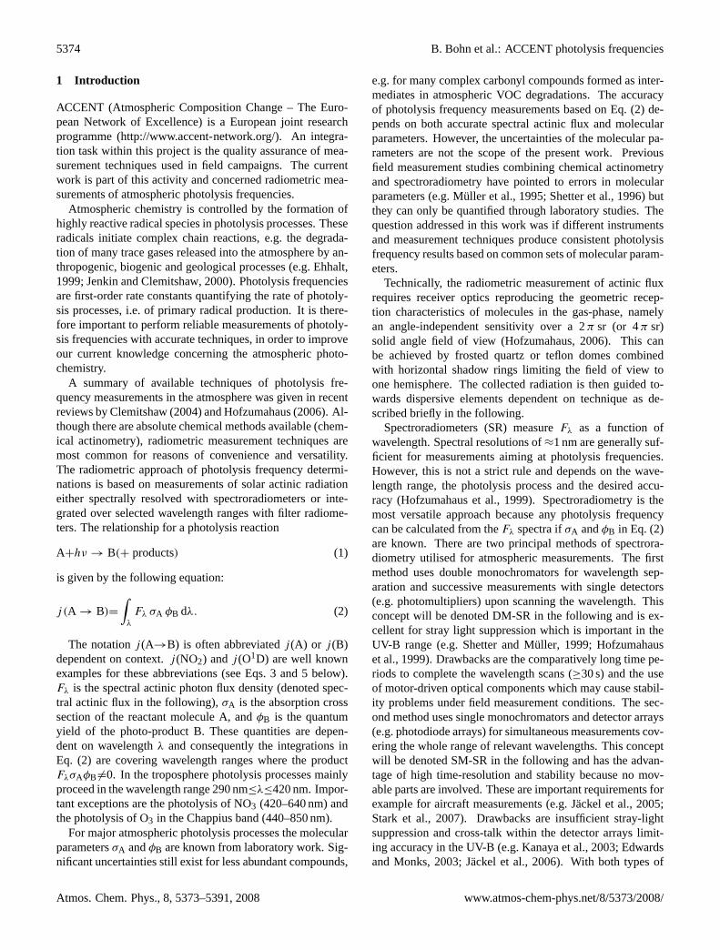


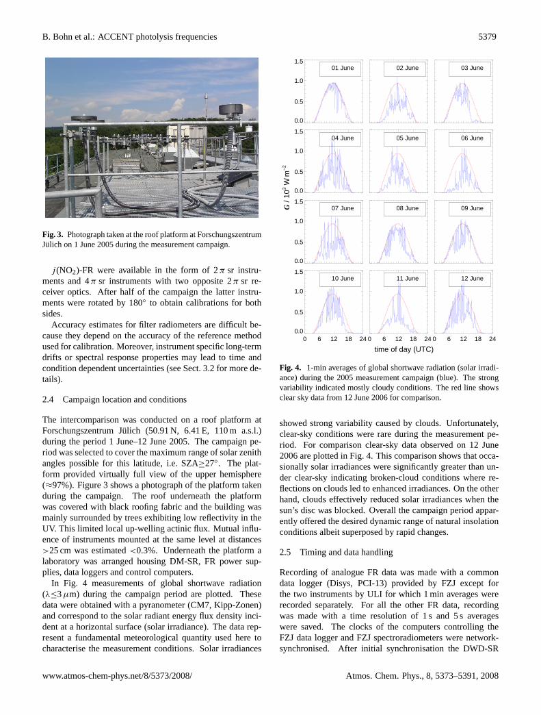

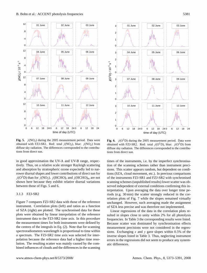


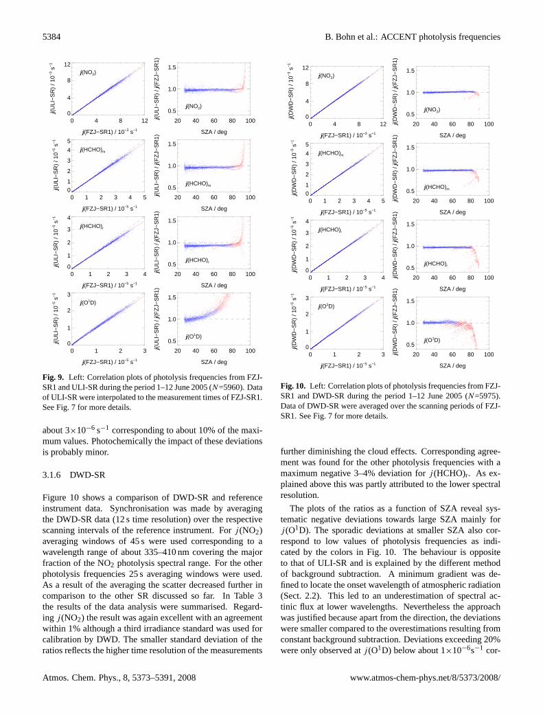


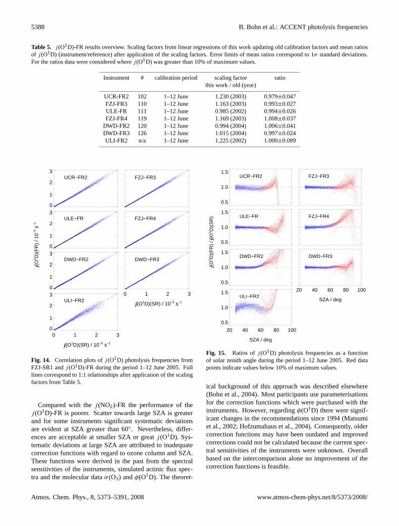


![Photolysis frequency of NO : Measurement and modeling ...russ/shetter_etal_2003.pdf[1] The photolysis frequency of NO 2, j(NO 2), was determined by various instrumental techniques](https://static.documents.pub/doc/80x56/5e7a9fbe414b0304c03c3cd3/photolysis-frequency-of-no-measurement-and-modeling-russshetteretal2003pdf.jpg)


![Impacts of aerosols and clouds on photolysis frequencies and ... of aerosols and cloud… · [2] Photolysis reactions play a very important role in atmospheric chemistry. Ozone photolysis](https://static.documents.pub/doc/80x56/5f07e35b7e708231d41f41d6/impacts-of-aerosols-and-clouds-on-photolysis-frequencies-and-of-aerosols-and.jpg)


