Abstract: We demonstrate the capabilities of principal componentanalysis (PCA) for studying the results of finite-difference time-domain(FDTD) algorithms in simulating photonic crystal microcavities. Thespatial-temporal structures provided by PCA are related to the actualelectric field vibrating inside the photonic microcavity. A detailed analysisof the results has made it possible to compute the phase maps for each modeof the arrangement at their respective resonant frequencies. The existenceof standing wave behavior is revealed by this analysis. In spite of this, somenumerical artifacts induced by FDTD algorithms have been clearly detailedthrough PCA analysis. The data we have analyzed are a given set of mapsof the electric field recorded during the simulation.
References and links1. E. Yablonovitch, “Inhibited spontaneous emission in solid-state physics and electronics,” Phys. Rev. Lett. 58,
2059-2062 (1987).2. P. R. Villeneuve, S. Fan, and J. D. Joannopoulos, “Microcavities in photonic crystals: mode symmetry, tunability,
and coupling efficiency,” Phys. Rev. B 54, 7837-7842 (1996).3. H. Y. Ryu and M. Notomi, “Enhancement of spontaneus emission from the resonant modes of photonic crystal
slab single-defect cavity,” Opt. Lett. 28, 2390-2392 (2003).4. C. Lixue, D. Xiaxou, D. Weiqiang, C. Liangcai, and L. Shutian, “Finite-difference time-domain analysis of
optical bistability with low treshold in one-dimensional non-linear photonic crystal with Kerr medium,” Opt.Commun. 209, 491-500 (2002).
5. A. Taflove and S. C. Hagness Computacional Electrodynamics: The Finite-Difference Time Domain Method, 2nded. (Artech House, Boston, 2000).
6. S. Guo and S. Albin, “Numerical techniques for excitation and analysis of defect modes in photonic crystals,”Opt. Express 11, 1080-1089 (2003); http://www.opticsexpress.org/abstract.cfm?URI=OPEX-11-9-1080
7. J. Jiang, J. Cai, G. P. Nordin, and L. Li, “Parallel microgenetic algorithm design for photonic crystal and waveg-uide structures,” Opt. Lett. 28, 2381-2383 (2003).
8. J. M. Lopez-Alonso, J. Alda, and E. Bernabeu, “Principal component characterization of noise for infrared im-ages,” Appl. Opt. 41, 320-331 (2002).
9. D. F. Morrison, Multivariate Statistical Methods, 3rd ed. (McGraw-Hill, Singapore, 1990), Chap. 8.10. J. M. Lopez-Alonso, and J. Alda, “Operational parametrization of the 1/f noise of a sequence of frames by means
of the principal components analysis in focal plane arrays,” Opt. Eng. 42, 427-430 (2003).11. R. B. Cattell, “The scree test for the number of factors,” J. Multivar. Behav. Res. 1, 245-276 (1966).12. D. D. Ghiglia and M. D. Pritt, Two Dimensional Phase Unwrapping(Wiley, New York, 1998), Chap. 4.13. A. Tredicucci, “Marriage of two device concepts,” Science 302, 1346-1347 (2003).
(C) 2004 OSA 17 May 2004 / Vol. 12, No. 10 / OPTICS EXPRESS 2176#4082 - $15.00 US Received 23 March 2004; revised 3 May 2004; accepted 3 May 2004
Since the late 1980s, after the publication of some seminal papers (for example, Ref. [1]), thenumber of experimental and numerical results on photonic crystal structures have increased.Among the wide variety of structures analyzed, photonic crystal microcavities [2] have becomea new tool for enclosing radiation. Some nontrivial phenomena—the modification of sponta-neous emission, the Kerr effect in photonic crystals [3, 4]—have been identified, and greateffort has been devoted to investigating and clarifying the causes of these facts. Numerical sim-ulations are essential tools for obtaining a deeper insight into the physics underlying photoniccrystal behavior. One approach that is often used is to solve Maxwell equations through a finite-difference time-domain numerical scheme (FDTD) [5]. Time-domain computations allow foran unambiguous characterization of important properties of microcavities, such as band-gapfeatures, resonant defect mode dynamics, and far-field pattern properties of crystal modes. Theresults have frequently been interpreted by use of fast Fourier transform analysis and filteringtechniques [6]. A complete numerical characterization of the photonic crystal is often required,guiding the design process. Furthermore, other numerical tools and optimization algorithms canbe incorporated into this process to improve and refine the final results [7].
Therefore, techniques for extracting useful information about mode characteristics should beavailable to photonic crystal researchers. In this paper, we propose applying a technique basedon principal component analysis (PCA) to analyze the results obtained from FDTD simula-tions of two-dimensional photonic crystal microcavities. PCA has been successfully employedfor analysis in image-processing systems and in noise characterization of cameras [8]. Herewe illustrate how PCA methods produce a more accurate determination of photonic crystalsproperties.
Section 2 explains the PCA analysis. In Section 3 we focus on the photonic crystal mi-crocavity that we have simulated. We have chosen a well-known system: a two-dimensionalphotonic crystal with a central defect [6]. The cavity is made of GaAs cylinders in air. It allowsthe presence of localized modes in the bandgap: the resonant modes of the system. They areexcited selectively by placing a specific set of point sources in different configurations. Thethree subsections developed here are devoted to the analysis of specific features of the electricfield distribution that remained unnoticed without the application of the PCA method. A spatialdistribution of the mode’s phase is computed in Subsection 3.1 as a consequence of the group-ing of couples of principal components with the same harmonic temporal evolution but shiftedπ/2 between them. Subsection 3.2 analyzes the meaning of another principal component thatappears systematically after the PCA action. Its electric field distribution is related to the exis-tence of a standing wave within the microcavity. Another interesting result derived from PCAis the capability to discern the presence of artifacts resulting from symmetry mismatch. Thiscapability is demonstrated in Subsection 3.3. Finally, Section 4 summarizes the main findingsof the paper.
2. Basis of the principal component analysis
PCA has demonstrated its utility for the classification and analysis of several sets of images.It is based on multivariate statistical techniques [9]. In our case, the input data are a set ofN frames containing maps of a given electromagnetic component regularly spaced in time,{F1,F2, . . . ,FN}, where Fi = F(ti), with ti the instants of time where the frames are taken. Eachframe contains M points arranged as one-, two-, or three-dimensional maps. If the map is notone dimensional, it is reshaped as a one-dimensional vector by a procedure that preserves theinformation about the actual location of each spatial point. The statistical variables are theelectromagnetic component at different time instants, Fi . They configure an N−dimensionalvariable, {Fi}. The M points define M realizations of the previously defined statistical variable.
(C) 2004 OSA 17 May 2004 / Vol. 12, No. 10 / OPTICS EXPRESS 2177#4082 - $15.00 US Received 23 March 2004; revised 3 May 2004; accepted 3 May 2004
The large number of statistical realizations usually available when analyzing irradiance mapsor electromagnetic field maps has made possible a clearer interpretation of the obtained data.Actual data exhibit nonnegligible correlations among frames. PCA generates a collection ofnew frames, or variables, that are uncorrelated. They are the so-called principal components,Yα , where α runs from 1 to N. These new variables are obtained by a diagonalization procedureapplied to the covariance matrix, S. The covariance matrix is calculated between frames. Then,S is a N×N matrix. The diagonalization procedure can be written as follows,
Seα = λα eα , (1)
where λ denotes the eigenvalues of this equation that represent the contributions of the principalcomponent with the same label, α ; and eα denotes the eigenvectors of the previous diagonal-ization. In addition, these eigenvectors are used to generate the principal components from theoriginal data,
Yα =N
∑i=1
eα (ti)F(ti). (2)
This last equation shows how the principal components can be written as a linear combinationof the original frames. In some manner, the PCA method can be seen as a linear change ofcoordinates. Moreover, the previous equation can be inverted to obtain the original frames fromthe principal components. When doing such a reconstruction, we can also limit or select theprincipal components. The result will be a filtered version of the original frames. This is alsoknown as principal component rectification.
The results of the PCA applied to N frames are N eigenvalues (λα ), N eigenvectors (eα ), andN principal components (Yα ). Each principal component can be arranged as a map having Mpoints. We may define them as eigenframes or eigenimages. The eigenvectors are orthogonaland represent the temporal evolutions of the contribution of each eigenimage to the originaldata. When describing frames with a given power spectrum density for a temporal-stationaryphenomena , PCA can be used to sample the spectrum and characterize it. The involved princi-pal components have quasi-harmonic time dependence [10]. Finally, the eigenvalues, explain indecreasing order the contribution of their associated principal component to the total varianceof the original data. It is also interesting to note that the capability of the PCA for sectioningthe variance and quantify the individual contributions of the obtained principal components tothe total variance of the original data, has made possible to reveal spatial-temporal structureshidden behind the main contributions to the variance of the data. To quantify this, we define thefollowing parameter,
wα =λα
∑Nα=1 λα
, (3)
where λα denotes the eigenvalues obtained from the PCA, and wα is the relative contributionof the given principal component, α , to the total variance of the data.
When we characterize noise within this multivariate technique, it is possible to associate anuncertainty to each eigenvalue [9]. This uncertainty is used to connect two consecutive eigen-values when their respective uncertainties overlap [8, 11]. Then a process is defined as theframes retrieved when only the principal components associated with consecutively overlappedeigenvalues are used. The concept of process is used to ease the interpretation of the resultsobtained from the PCA. The classification into processes reduces and groups the meaningfulprincipal components and provides an analytical tool that can be automatically applied andimplemented.
FDTD data are generated by computational algorithms that have been scrutinized and refinedover time to improve their output and make them more accurate and reliable. However, their
(C) 2004 OSA 17 May 2004 / Vol. 12, No. 10 / OPTICS EXPRESS 2178#4082 - $15.00 US Received 23 March 2004; revised 3 May 2004; accepted 3 May 2004
Fig. 1. Sequence of frames obtained for the photonic crystal analyzed in this paper andexcited to generate the monopolar mode. In all the figures of this paper, the grid nodescoincides with the centers of the cylinders of the microcavity (video file, 512 KB)
implementation will be affected by intrinsic limitations and constraints derived from the finiteand discretized realizations of the algorithm, both in time and in space. PCA has been proposedas a tool to identify and quantitatively estimate the presence of numerical artifacts and noise inthe FDTD output. An important feature of FDTD data is that the “signal” is much larger thanthe “noise.” In this case the signal is the primary source of the variance of the data. This fact,along with the decreasing importance of ordering of the eigenvalues, will identify the actualelectromagnetic field distributions with the first principal components. These “signal” principalcomponents may also be grouped into several processes according to the previously establishedmethod for defining a process. These features will be used and illustrated in the followingsections.
3. Photonic crystals analyzed by PCA
Our goal in this paper is to demonstrate the utility of PCA through a detailed study of a “bench-mark” example. A complete description of the simulated structure can be found in Ref. [6].For a better understanding we have followed the same choices and simulation parameters asthose used in Ref. [6]. The analyzed photonic crystal can support five modes, two of which aredegenerated. The resonance frequencies can be found in Ref. [6]. Simulations are two dimen-sional. The nonzero components of the electromagnetic fields are Ez, Hx, and Hy (this situationcorresponds to a TMz mode). We are going to excite some modes of the cavity in order to studythem with the PCA technique. By using this method, we will discriminate processes associatedwith different variance structures and we will ascribe them to relevant physical quantities of themodes. At this point, we should note this fact: PCA methods can be applied to any sequenceof frames and will be efficient in the analysis of any other photonic crystals. The dimensionallimitations are more related to the actual capabilities of the computing hardware. The PCAmethod is a blind tool that analyzes the structure of the variance of the data. Here the sourceexcitation methods, the size and location of the computational grid, or the geometry and natureof the spatial structure will not compromise the application of PCA. However, all these con-stitutive parameters and properties are necessary for properly understanding and analyzing thePCA results.
In the following subsection we will illustrate some of the most relevant features that havebeen obtained from the results of the PCA. In Fig. 1 we have represented the FDTD results for
(C) 2004 OSA 17 May 2004 / Vol. 12, No. 10 / OPTICS EXPRESS 2179#4082 - $15.00 US Received 23 March 2004; revised 3 May 2004; accepted 3 May 2004
Fig. 2. Semilog plot of the eigenvalues of each principal component after application of thePCA method to the sequence of frames shown in Fig. 1. The classification and groupingtechnique of the principal components can be applied by grouping together those principalcomponents that have consecutive overlapping in their respective uncertainties. We haveplotted the images corresponding to four principal components (numbers 20, 40, 60, and80) embedded in the same noise process.
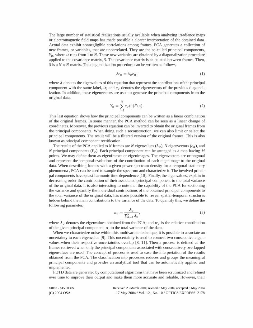
the monopolar mode of the simulated geometry. The computational spatial grid is composed of221× 221 nodes, the Courant factor is s= 0.7068, and the spatial step is δ = 0.025µm. Weobtained the data by selecting the electric field maps every 10 temporal steps. This rate guaran-tees that the temporal evolution is correctly sampled. The number of frames in the sequence ofdata is 101. In this case, the starting point for recording the data is placed after 40.000 temporalsteps. These results are in perfect accordance with the referenced results of Guo and Albin [6].Figure 2 represents the eigenvalues in a semilog plot. At the same time, we have applied theclassification method to group together those principal components with eigenvalues that areundistinguished. In this figure, we have also included the maps of some eigenimages (numbers20, 40, 60, and 80) belonging to the same process. This process makes up 0.00328% of the totalvariance. The temporal evolutions of the first principal components are shown in Fig. 3. Thequasi-harmonic dependencies are clearly visible. In this case, eigenvectors e1 and e2 oscillate asharmonic functions and are shifted π/2 one with respect to the other. This frequency is the sameas the monopolar mode frequency. In representing e1(t) versus e2(t), the points are located ona circle, thus validating the existence of the quasi-monochromatic process. The analysis of theeigenimages is left for the following subsections.
3.1. Phase map computation
The application of PCA for the analysis of noise figures made possible the definition of spatial-temporal processes that were obtained during analysis of the uncertainty and distinguishabilityof the eigenvalues obtained in the PCA application. These processes reduce the complexity ofthe variance structure by grouping together those structures that have eigenvalues with con-secutive overlapping uncertainties. The uncertainties themselves were obtained with statisti-cal techniques. On the other hand, the temporal evolution of the variance spatial structures,the eigenimages, are described by the associated eigenvectors. This fact was studied more indepth for finally relating the eigenvalues with sampled values of the power spectral density of agiven sequence of frames [10]. In that case, the eigenvectors showed a clear harmonic evolution
(C) 2004 OSA 17 May 2004 / Vol. 12, No. 10 / OPTICS EXPRESS 2180#4082 - $15.00 US Received 23 March 2004; revised 3 May 2004; accepted 3 May 2004
Fig. 3. The temporal evolution of the principal component is described by the associatedeigenvectors. In this figure we plot the first three eigenvectors obtained from the PCAmethod. They show an harmonic dependence. In (a) we plotted the first two eigenvectors,which show the same temporal frequency but shift π/2. Image (b) corresponds to the thirdeigenvector. When representing e2 versus e1, in (c), we can check that the frequency is thesame and that the relative phase delay is π/2.
that allowed a temporal frequency interpretation. In the case analyzed in this paper, we havefound some other connections between the temporal evolution of the eigenvectors. These find-ings have been interpreted within the scope of the electromagnetic computations performed bythe FDTD methods. Then we have proposed grouping together those eigenimages associatedwith eigenvectors that have the same frequency in their quasi-harmonic temporal evolution.As shown below, this association is made in couples. Moreover, their temporal evolutions areshifted π/2 one with respect to the other. This is the only solution for the eigenvectors to remainorthogonal at the same frequency [10]. Therefore, we may propose the existence of “quasi-monochromatic processes” formed by the eigenvectors (and their associated eigenimages andeigenvalues) with the same temporal frequency.
A relevant feature obtained from the PCA for the photonic crystal study is that two principalcomponents, Ya and Yb, are associated with eigenvectors that oscillate at the same frequency butshifted π/2 one eigenvector with respect to the other. Although they are not connected by theirrespective eigenvalues’ uncertainties, we could still generate a collection of frames by recon-structing a filtered version of the original data with only these two principal components. Theresulting spatial-temporal structure is the “quasi-monochromatic process” of the kind proposedin the previous paragraph. This process usually represents a large amount of the total varianceof the original data. The reconstruction of the original data with these two eigenvectors can bewritten as follows,
Fa,b(x,y, t) = ea(t)Ya(x,y)+eb(t)Yb(x,y), (4)
where the superindex a,b stands for the two principal components involved in the calculation.The eigenvectors, ea and eb, are given by
(C) 2004 OSA 17 May 2004 / Vol. 12, No. 10 / OPTICS EXPRESS 2181#4082 - $15.00 US Received 23 March 2004; revised 3 May 2004; accepted 3 May 2004
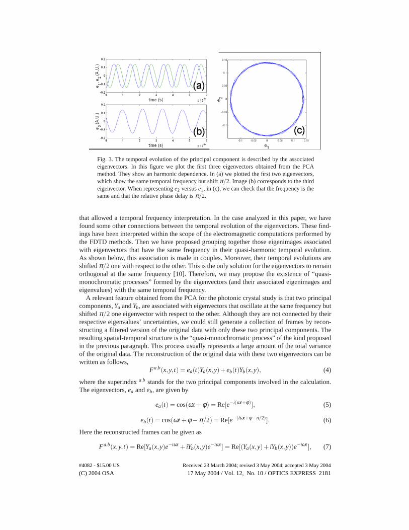
Fig. 4. On the left-hand side we show the sequence of frames (video file 495 KB) obtainedby reconstructing the data with only Y1(x,y) and Y2(x,y) for the original data presented inFig. 1. This result can be considered as a filtered version of the FDTD output that con-tains 99.98701% of the total variance of the original data. The mode observed here is themonopolar one. On the right-hand side we present the difference between the original andthe filtered version (video file 809 KB).
where we set φ = 0 without loss of generality. Equation (7) defines a complex principal com-ponent, Ya,b, that deserves special attention. Alternatively, it can be written as follows,
The phase of this principal component shows temporal and spatial dependence. The previousdevelopment is based on the linear character of the Maxwell’s equations and the media involvedin the calculation.
As illustrated above, the application of the PCA method to FDTD data, obtained for awell-referenced photonic crystal simulation that generates a monopolar mode, has produceda couple of eigenvectors with quasi-harmonic dependence. They can be grouped into a “quasi-monochromatic” process. From the results of the simulation this process represents 99.98701%of the total variance of the original data. In Fig. 4 (left), we show the results after reconstruct-ing the frames with only the quasi-monochromatic process, F1,2(x,y, t), following Eq. (9). Thismovie can be seen as a filtered version of the original data obtained directly, without any otherfiltering technique, from the FDTD algorithm. The difference between the original and thePCA-filtered data is also included in this figure. It contains two main features. In the center, wecan observe a high-frequency evolution. These patterns were also plotted in Fig. 2 and shouldbe associated with noise processes. The other feature will be explained in the next subsection.
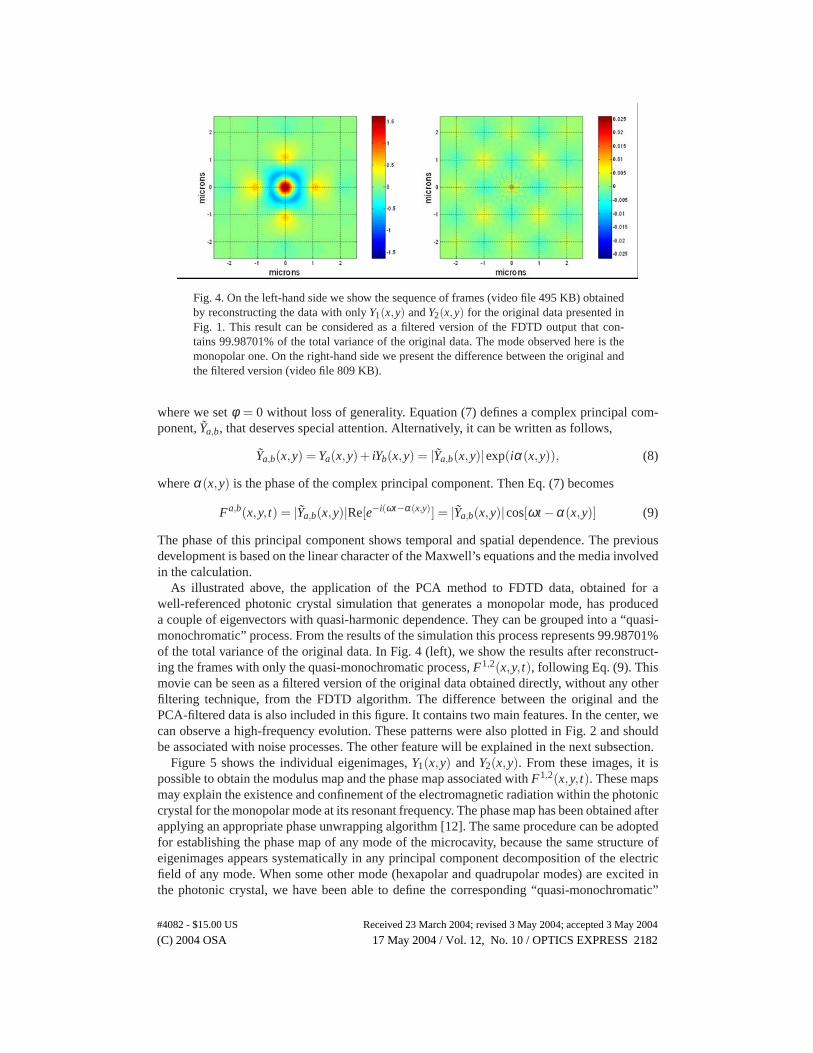
Figure 5 shows the individual eigenimages, Y1(x,y) and Y2(x,y). From these images, it ispossible to obtain the modulus map and the phase map associated with F1,2(x,y, t). These mapsmay explain the existence and confinement of the electromagnetic radiation within the photoniccrystal for the monopolar mode at its resonant frequency. The phase map has been obtained afterapplying an appropriate phase unwrapping algorithm [12]. The same procedure can be adoptedfor establishing the phase map of any mode of the microcavity, because the same structure ofeigenimages appears systematically in any principal component decomposition of the electricfield of any mode. When some other mode (hexapolar and quadrupolar modes) are excited inthe photonic crystal, we have been able to define the corresponding “quasi-monochromatic”
(C) 2004 OSA 17 May 2004 / Vol. 12, No. 10 / OPTICS EXPRESS 2182#4082 - $15.00 US Received 23 March 2004; revised 3 May 2004; accepted 3 May 2004
Fig. 5. In this figure we have plotted the spatial maps of the electric field associated withthe first two principal components, Y1(x,y) (top left) and Y2(x,y) (top right), obtained fromthe simulation carried out for the monopolar mode. It is possible to evaluate the modulus(bottom left) and the phase(bottom right) of the complex eigenimage associated with theseprincipal components.
processes that allow the calculation of the distribution associated with each one of the modes.The determination of the modulus and the phase related to these modes are presented in Fig. 6.
3.2. Standing waves
Another interesting result is related to the characteristics of those principal components havingquasi-harmonic dependence in their temporal evolution that can not be grouped with anotherprincipal component to form a “quasi-monochromatic” process. The associated eigenvectorsare quasi-harmonic and are characterized by a given temporal frequency. No other principalcomponent shows temporal evolution with quasi-harmonic dependence at the same frequency.Typically, the temporal frequency of the associated eigenvector falls in the tails of the spectrumfor some of the modes of the photonic crystal. These structures are labelled as standing waves.In some other previous contribution it has been stated the presence of stationary waves withinthe structure of photonic crystals [13].
In the analyzed examples, the frequencies of the standing waves are located outside the bandgap of the structure[6]. The band-gap comprises frequencies between 0.29 c
a and 0.42 ca , where c
is the speed of light and a is the lattice constant of the crystal. We have simulated three modes:monopolar, one of the quadrupolars, and the hexapolar. The standing waves only appear distin-guished from noise for the monopolar and the hexapolar modes computations. In the monopolarcase, the frequency of the standing wave is 0.281 c
a , that is smaller than the lower limit of thebandgap. Moreover, for the hexapolar case, the frequency, 0.57 c
a , is higher than the upper limit
(C) 2004 OSA 17 May 2004 / Vol. 12, No. 10 / OPTICS EXPRESS 2183#4082 - $15.00 US Received 23 March 2004; revised 3 May 2004; accepted 3 May 2004
Fig. 6. Spatial distribution of the modulus and the phase associated with the “quasi-monochromatic” processes obtained for the hexapolar (left column) and one of thequadrupolar (right column) modes of the photonic crystal analyzed in this paper.
of the bandgap. This is because the tails of the monopolar and hexapolar spectra spread outsidethe band gap with a non-negligible amplitude. This is not the case for the quadrupolar mode,whose tails outside the bandgap are negligible [6].
In order to assure that these processes are actually present in the spatial-temporal evolutionof the data, we have performed several simulations by using excitation sources with the charac-teristic temporal frequency of the obtained eigenvector. The results have always produced onlyone principal component having such a temporal evolution. For the monopolar mode, the PCAhas produced a principal component, Y3(x,y), that shows a harmonic dependence, e3(t) (seefigure 3.b). The contribution of this third principal component to the total variance of the datais only w3 = 0.00971%. Then, the presence of this oscillation may be swept out by any filteringtechnique applicable to the original data. On the other hand, the spatial distribution is quiteremarkable and resembles the geometrical arrangements of the photonic crystal. Besides, theassociated eigenvector follows a quasi-harmonic dependence. When reconstructing a filtered setof frames by using only this principal component, we may observe the typical behavior of anstanding wave (see left map in Fig. 7). The nodes are also located in good accordance with thesymmetry of the arrangement. The modulus of the instantaneous Poynting vector is displayedin the center of figure 7. This plot suggests that the energy is trapped at the cylinders’ locations.The hexapolar mode has produced another standing wave principal component, Y3(x,y) (seeright map of figure 7). Its contribution to the total variance is 0.00569%. The symmetry of thisstanding wave is driven by the symmetry of the hexapolar mode and it is again attached to the
(C) 2004 OSA 17 May 2004 / Vol. 12, No. 10 / OPTICS EXPRESS 2184#4082 - $15.00 US Received 23 March 2004; revised 3 May 2004; accepted 3 May 2004
Fig. 7. On the left we show the temporal evolution of the frames rectified by using only thestanding wave principal component excited when the monopolar mode is fed at the centerof the structure (video file 975 KB). The modulus of the instantaneous Poynting vectoris displayed in the central map. The plot on the right corresponds to the standing waveobtained for the hexapolar mode excitation.
Fig. 8. Spatial distribution of one of the principal components obtained for a decenteredexcitation of the monopolar mode. The spatial distribution closely resembles much thehexapolar mode that is generated when the excitation is not centered. The temporal evolu-tion given by the associated eigenvector also coincides with the hexapolar mode frequency.The relative contribution to the total variance of this principal component is 0.0017%.
central cylinder structure.
3.3. Decentering artifacts
The analysis of the computational noise generated by the FDTD algorithms is also possible.One of the most striking results of the usefulness of the PCA has been obtained when themonopolar mode of the analyzed photonic crystal is generated within a two dimensional gridwith even number of nodes along the orthogonal directions. In such case, the excitation cannot be precisely located at the center of the photonic crystal. The excitation frequency is thatone of the monopolar mode. However, the application of the PCA has produced as a secondaryprocess the excitation of noncentered modes, as the hexapolar one. The monopolar mode isstill the most contributing one, but a detailed analysis of the obtained eigenimages has revealedthe presence of another oscillation, clearly linked with the lack of centration of the excitationwithin the two-dimensional grid. This oscillation follows the spatial and temporal pattern of thehexapolar mode (see Fig. 8).
(C) 2004 OSA 17 May 2004 / Vol. 12, No. 10 / OPTICS EXPRESS 2185#4082 - $15.00 US Received 23 March 2004; revised 3 May 2004; accepted 3 May 2004
The use of FDTD techniques for simulating the interaction of electromagnetic fields with ma-terial structures has become a well-established tool for the analysis of photonic crystals. WhenPCA techniques are applied to the temporal evolution of the maps of electromagnetic magni-tudes, the obtained results reveal spatial-temporal structures that can be interpreted and linkedwith the actual geometrical and constitutive properties of the photonic crystals. In this paper,we have demonstrated the pertinence of such analysis of FDTD results. The outputs of the PCAmethod have been interpreted as follows: the eigenimages represent maps of electromagneticfields (here, the electric field and the Poynting vector); the eigenvectors represent temporal evo-lutions linked with the expected harmonic variations of the modes of the photonic crystal; andthe eigenvalues represent their contribution to the total variance of the original data.
PCA allows an easy classification and grouping of the principal component into processes.When the classification of these processes is made in terms of eigenvalue distinguishability,the number of principal components associated with physically meaningful maps is drasticallyreduced, providing a simple tool for cleaning and filtering the FDTD results. Inasmuch as thePCA analyzes the correlation structure of the data, some spatial-temporal patterns with differentcorrelations are distinguished. Furthermore, these structures with some correlation are extractedfrom the noise itself. When PCA is applied to the photonic crystal analysis, it has produced threetypes of spatial-temporal patterns. The first one is a “quasi-monochromatic” process relatedto the defect modes of the photonic crystal. It gives the resonant frequency, and the spatialdistribution of its modulus and phase. The second one has been interpreted as a standing wavelinked to the geometry and symmetry of the microcavity and the mode. Their frequencies falloutside the bandgap. Finally, the third spatial-temporal pattern can be interpreted as numericalnoise. Some of the spatial-temporal structures with physical meaning contribute with muchless than 1% to the total variance; however, their spatial shape and their temporal evolutiondenote inner relations that can be properly determined. In this case, they could be swept out byconventional filtering techniques.
When symmetric structures are simulated with symmetric calculation grids, special attentionhas to be paid to the matching of these symmetries. PCA has shown that even a minimumdecentering may provoke the excitation of other modes of the photonic crystal. Owing to thenegligible contribution to the total variance of that mode, it is not surprising that the applicationof any other filtering technique hides and erases the existence of those decentering artifacts.However, PCA has revealed them and quantified their importance. Moreover, some other subtleeffects and interpretations are possible by a dedicated analysis of the data.
Acknowledgments
This research has been supported by the project “Optical Antennas,” TIC2001-1259, financedby the Ministerio de Ciencia y Tecnologıa of Spain.
(C) 2004 OSA 17 May 2004 / Vol. 12, No. 10 / OPTICS EXPRESS 2186#4082 - $15.00 US Received 23 March 2004; revised 3 May 2004; accepted 3 May 2004