Phylogenetics

Tanmoy Bhattacharya

Los Alamos National Laboratory

4th qBio Summer School

July 28, 2010

outline

1. Inference in historical sciences.2. State versus Process.3. Importance of Time Scales.4. Maximum Likelihood and Bayesian.5. Information Criteria.6. Example from HIV:

I Getting the tree.I Using the tree: timing.I Using the tree: population history.I Using the tree: counting.I Practical uses.

7. Conclusions.

Science and repeatabilityThese steps must be repeatable in order to dependably predict any future results. (Wikipaedia)

The Book of Optics by Ibn al-Haytham (1021): consciousreliance upon repeated observations to infer regularities.

Repeated observations can come from:I Performing controlled experiments, orI Selecting from a stream of data.

Small correlation structure leads to independent observations.

History may have long correlations: not independent.

I Cosmic Variance: the problem of one universe.

I Large planets have lower density: rule?

I Widespread language similarities: cognitive structure?

I Four limbs: adaptation?

I Similarity across religions: common truth?

Galton’s Problem

Ought we ... to begin by discussing each separate species—man, lion, ox, and the like—taking each kind in handindependently of the rest ... (De partibus Animalium)

In 1889 Sir Edward Tylor presented a paper on correlationsbetween marital systems and societal complexity.

Sir Francis Galton pointed out confounding by borrowing andcommon descent.

General problem of dealing with autocorrelation called Galton’sproblem by Raoul Naroll in 1961.

If the cause of the correlation is known, one can reduce it byvarious methods: data selection, multiple regression, orlagging.

How do we know what is independent?

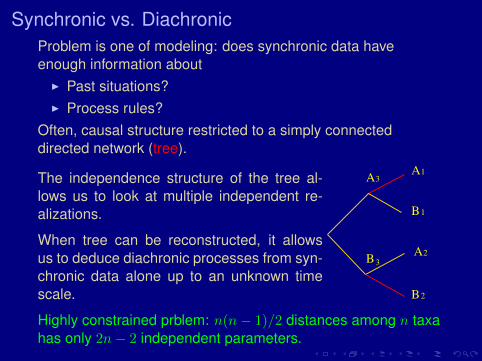
Synchronic vs. DiachronicProblem is one of modeling: does synchronic data haveenough information about

I Past situations?I Process rules?

Often, causal structure restricted to a simply connecteddirected network (tree).

The independence structure of the tree al-lows us to look at multiple independent re-alizations.

When tree can be reconstructed, it allowsus to deduce diachronic processes from syn-chronic data alone up to an unknown timescale.

3

B

A

B

A

B

A

2

2

1

1

3

Highly constrained prblem: n(n− 1)/2 distances among n taxahas only 2n− 2 independent parameters.

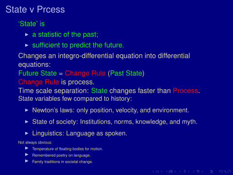
State v Prcess‘State’ is

I a statistic of the past;I sufficient to predict the future.

Changes an integro-differential equation into differentialequations:Future State = Change Rule (Past State)Change Rule is process.Time scale separation: State changes faster than Process.State variables few compared to history:

I Newton’s laws: only position, velocity, and environment.

I State of society: Institutions, norms, knowledge, and myth.

I Linguistics: Language as spoken.Not always obvious:

I Temperature of floating bodies for motion.I Remembered poetry on language.I Family traditions in societal change.

Branching Processes

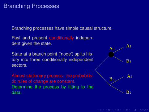
Branching processes have simple causal structure.

Past and present conditionally indepen-dent given the state.

State at a branch point (‘node’) splits his-tory into three conditionally independentsectors.

Almost stationary process: the probabilis-tic rules of change are constant.Determine the process by fitting to thedata.

3

B

A

B

A

B

A

2

2

1

1

3

Timescales

Example:I Large number of almost independent traits.I Varying at different rates.I Rates constant, though different for different traits.

Fast Traits

2

B

A

B

A

B

A

2

2

1

1

3

3

1C

C

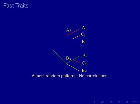
Almost random patterns. No correlations.

Slow Traits

2

B

A

B

A

B

A

2

2

1

1

3

3

1C

C

Essentially constant. Replicated initial conditions.

Informative Traits

2

B

A

B

A

B

A

2

2

1

1

3

3

1C

C

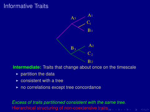
Intermediate: Traits that change about once on the timescaleI partition the dataI consistent with a treeI no correlations except tree concordance

Excess of traits partitioned consistent with the same tree.Hierarchical structuring of non-coextensive traits.

Hierarchical Structure

Fast Random Traits

Hierarchical Structure

Implicational scaling

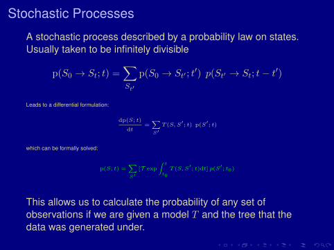
Stochastic Processes

A stochastic process described by a probability law on states.Usually taken to be infinitely divisible

p(S0 → St; t) =∑St′

p(S0 → St′ ; t′) p(St′ → St; t− t′)

Leads to a differential formulation:

dp(S; t)

dt=

∑S′T (S, S

′; t) p(S

′; t)

which can be formally solved:

p(S; t) =∑S′

[T exp

∫ t

t0

T (S, S′; t)dt] p(S

′; t0)

This allows us to calculate the probability of any set ofobservations if we are given a model T and the tree that thedata was generated under.

Forward process; Backward inferenceModel is constant! How do we determine it?

I Choose model parameters.I Forward: Either simulate or calculate expected

observations.I Evaluate how expected the actual observations are.I Backward: Vary model and choose best.

How does this perform with large amount of independent data?True Model M : Independent observations with prbability {pi}.Observation i seen with frequency fi ≈ pi.

Let model Mj assign it probablities pij . Log Total probability

lnL(Mj) ≡ ln p(Data |Mj) =∑i

fi ln pij .

Maximize over j subject to∑

i pij = 1: pij = fi.

The model chosen by Maximum Likelihood is consistent.

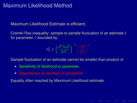
Maximum Likelihood Method

Maximum Likelihood Estimate is efficient.

Cramer-Rao inequality: sample-to-sample fluctuation of an estimate bfor parameter β bounded by:

σ2b ≥

(∂2 lnL∂β2

)−1⟨∂b

∂β

⟩2

.

Sample fluctuation of an estimate cannot be smaller than product of

I Sensitivity of likelihood to parameter.

I Dependence of estimate on parameter.

Equality often reached by Maximum Likelihood estimate.

Example

Toss a loaded coin many times: how do we determineprobability of heads?

As the probability of heads increases, the fraction of headsincreases. So, does the number of runs of heads.

Can use different features of the data, e.g.,I Fraction of heads.I Average length of runs of heads.

Maximum likelihood chooses fraction of heads, because it ismost informative.

Similarly, no need to sort out non-informative fast and slowtraits: Maximum Likelihood method weights each trait at itsproper time depth.

Model misspecification

Likelihood based methods are ideal ifI There is enough data.I Model in the specified class.

When model does not allow features of the data: one can getbizarre results.Model: Bengali derived from the Vedic language of India.We want to find how long back Vedic was spoken.If we do not recognize that many modern words are actuallyfrom Persian, English, Portuguese, Dravidian, Austrasiatic, etc.,we will get a very wrong answer.But, if we allow a probability for random new word: we startgetting reasonable results.Rare forgotten processes can sometimes be replaced byuncorrelated random processes.

Likelihood RatioFor Normal distribution, −2 lnL ≡ χ2 +

∑ln(2πσ2).

I Maximum Likelihood is a generalization of minimum χ2.I Provides confidence intervals.

Adding parameters gives better fit even at random.Best fit models with δ more parameters: 2∆ lnL ∼ χ2

δ .I Quantifies overfitting.

This can be generalized to Bayesian posterior

p(Mi | Data) ∝ p(Mi)L(Mi) .

I Can incorporate prior knowledge.I Penalizes extra parameters more.I Can be evaluated by a Markov Chain Monte Carlo.

Markov Chain Monte CarloHow to sample a random distribution?Replace ensemble average by time average. Choices:

1. Design a deterministic ergodic process.2. Use Markov processes.

If there is a random Markov process, p(X → Y ), such thatI p(X→Y )

p(Y→X) = π(Y )π(X) ,

I Every state is reachable in one or more moves,I The process is not periodic, andI The expected number of moves to return is finite,

Then, this ergodic process samples X in proportion to π(X).Much easier problem because p(X → Y ) is local.Example:

I Choose a small neighbourhood {Xj} for each Xi.

I Choose p(Xi → Xj) = 1 if π(Xj) > π(Xi).

I Choose p(Xi → Xj) = π(Xi)/π(Xj) otherwise.

I Check the criteria.

Information Criteria

How do we decide when a richer model should be used?

Three problems with increasing parameters:I More parameters make estimation more noisy.I More parameter models more sensitive to noisy estimates.I Many more multiparameter models to choose from:

fairness?

Akaike Information Criterion: Choose number of parameters tomaximize predictability.Bayesian Information Criterion: Use a prior on number ofparameters; minimize unassumed coincidences.

Akaike Information Criterion

Two parts:I Parameter fits non-reproducible noise.I Parameter mispredicts future observations.

Let,I θ be the true model,I X be some observations,I Y be similar future observations.

Let θX be the model estimated from X: i.e., the model thatmaximizes the likelihood L(θX |X). But, what we really want is amodel that assigns high probability p(Y ) to future observations.

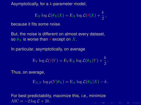
Asymptotically, for a k-parameter model,

EX logL(θX |X) = EX logL(θ|X) +k

2,

because it fits some noise.

But, the noise is different on almost every dataset,so θX is worse than θ except on X.

In particular, asymptotically, on average

EY logL(θ|Y ) = EY EX logL(θX |Y ) +k

2.

Thus, on average,

EX,Y log p(Y |θX) = EX logL(θX |X)− k .

For best predictability, maximize this, i.e., minimizeAIC ≡ −2 logL+ 2k.

Bayesian Information Criterion

Data can’t prove a hypothesis: it can rule it out.

Bayesian prior: how much support from data do we need torule out the hypothesis?

Uniform prior: Each hypothesis has equal a priori probability= 1/Number of hypothesis.

If lower parameter model a point in higher parameter space:zero a priori probability; needs infinite data to override!

Use distributions (Dirac δ functions): total probability of lowerparameter model equal to total probability of higher parametermodel.

This is equivalent to letting data resolution decide the ‘size’ ofthe lower dimensional point.

If data sample is of size n, error bars are size 1/√n. So, a k

lower-dimensional point has relative volume exp−k2 log n.

Equal probability means, lower dimensional model hascorrespondingly larger a priori weight compared to every pointin the higher dimension: so, choosing a higher parametermodel requires that much more evidence.

So, to maximize Bayesian posterior, minimizeBIC ≡ −2 logL+ k log n.

Since sample size arbitrary: being just able to rule out lower dimensional model is surprising. BIC requires that the

fit be better in proportion to data.

Example: phylogeny in biologyCan one use these methods to infer history of life? Is history oflife tree-like?

But history of what?

Traits are inherited

I From parents.

I From peers.

I From physical environment.

I From previous changes in environment . . . .

Look for a large co-inherited bundle of traits. Define this as‘vertical transmission.’ Other inheritences referred to thisbaseline.

One such large bundle: genetic traits.

Genotype

Most of life has a strong genotype-phenotype separation.

I Genotype encodes heredity: phenotype is selectable.I Genotype to phenotype program not easily invertible.I Genotype changes mainly dictated by chemistry: almost

stationary process.

Genotype changes randomly, weakly filtered by selection. Vastamount of almost independent traits, almost stationary process.

I Most of life close to fitness maximum.I Robustness: Few changes fatal, most neutral.I High mutation rates harmful.

(Eigen’s law: no more than 1 change/unit/generation.)I Mutation rate maximized for adaptability.

Genetic Change

Most of the changes are ‘point mutations’:

GTAAGACAGTATGATCAGATACTCATAGAAATCTGTGGA →GTAAAACAATATGATCAGGTATCTATAGAAATTTGTGGA .

Some regions are prone to insertions or deletions.

AGTAATACTACTAGTAAT ↔ACT ATACTA AAT .

Daughter may form from parts of different parents

...AGGATGGAC...

...TTTATGCTG...→ ...AGGATGCTG...

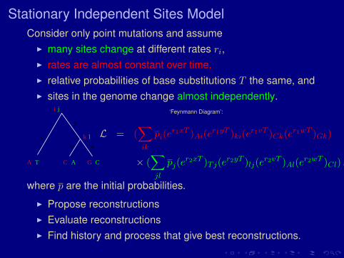
Stationary Independent Sites ModelConsider only point mutations and assume

I many sites change at different rates ri,I rates are almost constant over time,I relative probabilities of base substitutions T the same, andI sites in the genome change almost independently.

T A CA C G

i

k

j

lx

y

v w

‘Feynmann Diagram’:

L = (∑ik

pi(er1xT )Ai(e

r1yT )ki(er1vT )Ck(e

r1wT )Gk)

× (∑jl

pj(er2xT )Tj(e

r2yT )lj(er2vT )Al(e

r2wT )Cl) ,

where p are the initial probabilities.

I Propose reconstructionsI Evaluate reconstructionsI Find history and process that give best reconstructions.

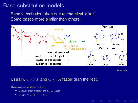
Base substitution modelsBase substitution often due to chemical ‘error’.Some bases more similar than others:

Wikimedia

Usually, C ↔ T and G↔ A faster than the rest.

The calculation simplifies further ifI p is stationary distribution: Tp = 0, andI Tijpj = Tjipi ∀i, j.

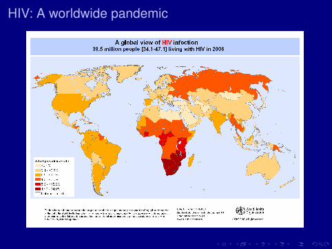
HIV: A worldwide pandemic

HIV: A social problemAffects the sexually active (productive) age group.

Destroys families: orphans and the aged.

Asymptomatic phase before AIDS: 9 years untreated.

Escapes single drugs within a couple of days. Escapes doublecombinations in years.

Prevention difficult

I lifestyle changes (e.g.,monogamy, condoms,circumcision)

I screening bloodI sterilizing needlesI expensive drugs

Medipedia

HIV: The VirusWe knowthe structure, the function,

Adcock Ingram

the genetics,

HIV Database

and the infection dynamics.

McMichael et al.,Nat. Rev. Immun. 2010 Jan; 10(1):11–23.

HIV: Extreme DiversityNo effective vaccine yet!

HIV InfluenzaArcher and Robertson, Smith et al.,

AIDS 2007 Aug 20; 21(13):1693–1700 Science 2004 Jul 16: 305(5682):371–376

Need to understand biology and evolution.

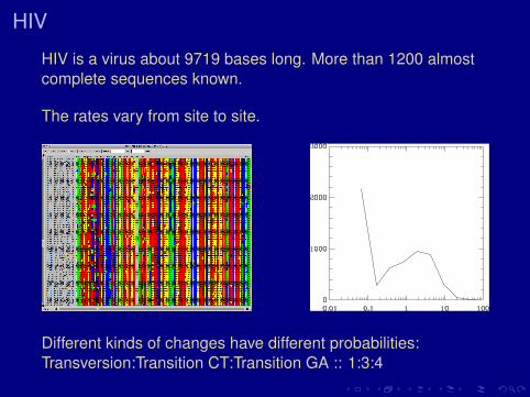
HIV

HIV is a virus about 9719 bases long. More than 1200 almostcomplete sequences known.

The rates vary from site to site.

Different kinds of changes have different probabilities:Transversion:Transition CT:Transition GA :: 1:3:4

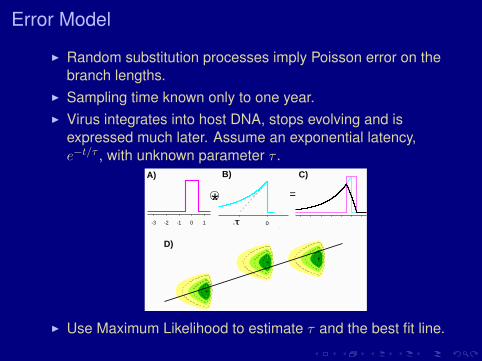
Error Model

I Random substitution processes imply Poisson error on thebranch lengths.

I Sampling time known only to one year.I Virus integrates into host DNA, stops evolving and is

expressed much later. Assume an exponential latency,e−t/τ , with unknown parameter τ .

B)

-3 -2 -1 0 1 - 0

=*τ

A) C)

D)

I Use Maximum Likelihood to estimate τ and the best fit line.

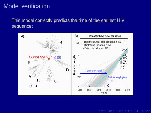
Model verification

This model correctly predicts the time of the earliest HIVsequence:

F

0.10

1959

C

CONSENSUS

B

D

HJA

A) B)

Bra

nch

Leng

th .15

Year

.05

.10

Best fit line, real data excluding ZR59Bootstraps excluding ZR59Data point, all post-1983

Test case: the ZR1959 sequence

1957

ooo

o

o

o

o

oo

o

o

o

o

o

o

oo

o

oo

o

o

o

o

o

o

o

o

o

o

o

o

o

o

o

o

o

o

o

o

o

o

o

oo

o

o

o

o

oo

o

o

o

o

o

o

o

o

o

o

o

o

o

o

o

o

o

o

o

oo

o

o

o

o

o

o

o o

o

oo

o

o

o

o

o

oo

o

o

o

o

o

o

oo

o

o

o

o

o

o

o

o

o

o

o

oo

oo

oo

o

o

oo

o

oo

o o

oo

o

o

o

o

o

o

o

o

o

o

o

o

o

o

o

1900 1920 1940 1960 1980 20000

.20

Predicted sampling time

ZR59 branch length

o

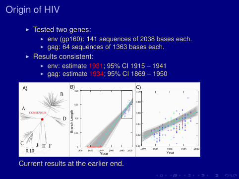
Origin of HIV

I Tested two genes:I env (gp160): 141 sequences of 2038 bases each.I gag: 64 sequences of 1363 bases each.

I Results consistent:I env: estimate 1931; 95% CI 1915 – 1941I gag: estimate 1934; 95% CI 1869 – 1950

0.14

0.16

0.18

0.12

A)

C

A

Year

Bra

nch

Length

0.10HJ

B) C)

CONSENSUS

B

D

F 0

0.05

0.15

0.10

C

A

C

A

C

B

A

B

B

B

CB

B

B

B

B

B

B

C

F

C

B

B

B

A

C

B

B

B

B

J

B

C

C

CFD

B

B

B

B

C

D

B

B

C BC

A

B

B

B

B

C

C

A

D

A

F

C

F

C

A B

B

D

C

CB

B

B

C

D

B

A

B

H

C

B

D

B

B

BB

B

B

A

B

A

B

B

D

B

B

C

B

B

A

A

A

C

JB

D

D

B

B

B

C

B

C

B

B

B

B

B

D

B

D

B

D

B

B

C

B

B

B

B

A

C

B

B

B

B

C

BB

B

B

D

B

1900 1920 1940 1960 1980 2000

0.20 0.20

2000

Year

C

A

C

A

C

B

A

B

B

B

CBB

BB

B

B

BC

F

C

B

B

B

A

C

B

B

B

B

J

B

C

C

CFD

B

B

B

B

C

D

B

B

C BC

A

B

B

B

B

C

C

A

D

A

F

C

F

C

A B

B

D

C

CB

B

B

C

D

B

A

B

H

C

B

D

B

B

BB

B

B

A

B

A

B

B

D

B

B

C

B

B

A

A

A

C

JB

D

D

B

B

B

C

B

C

B

B

B

B

B

D

B

D

B

D

B

B

C

B

B

B

B

A

C

B

B

B

B

C

BB

B

B

D

B

1980 1985 1990 19950.10

Current results at the earlier end.

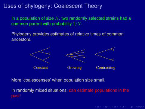
Uses of phylogeny: Coalescent Theory

In a population of size N , two randomly selected strains had acommon parent with probability 1/N .

Phylogeny provides estimates of relative times of commonancestors.

ContractingConstant Growing

More ‘coalescenses’ when population size small.

In randomly mixed situations, can estimate populations in thepast!

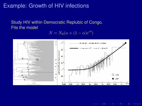
Example: Growth of HIV infections

Study HIV within Democratic Replubic of Congo.Fits the model

N = N0(α+ (1− α)ert)

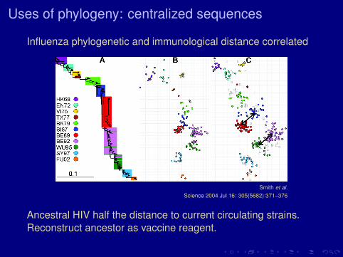
Uses of phylogeny: centralized sequences

Influenza phylogenetic and immunological distance correlated

Smith et al.Science 2004 Jul 16: 305(5682):371–376

Ancestral HIV half the distance to current circulating strains.Reconstruct ancestor as vaccine reagent.

Uses of phylogeny: A Problem in HIV immunologyCytotoxic T Lymphocytes (CTL) recognize and kill virallyinfected cells.

Small bits of virus presented for recognition by class I HumanLeukocyte Antigen (HLA).

Halling-Brown, Ph.D. Thesis

3�

2� 1�

�-microglobulin

en.wikipaedia:atropos235

Which bits of the virus (epitopes) are recognized by CTLs?

Solution

Direct SolutionFind the HLA type of the individual.Find sequence positions where change is selected over time.Construct overlapping stretches of small peptides.Study binding.

Statistical Solution

Individuals differ in HLA.If an epitope recognized, it may escape by changing.Study a population and HIV extracted from them.If an HIV sequence position correlates with host HLA, it is likelyto be in an epitope.

Incorrect Results!!!

89/202 (37–51%) positions in the protein Pol correlated withhost HLA.

11 (3–10%) significant even after correction for multiple tests.Moore et al., Science 2002 296:1439–1443.

A separate study: 346/624 (51–59%) positions correlated.

80 (10–16%) significant with a cutoff on false positive rate of20%. Kiepiela et al., Nature 2004 432:769–775.

Conclusion:CTL escape significant factor in shaping HIVevolution.

C*1701

Dataset from Perthdominated by B subtype.

All C*1701+ people in thedataset are C subtypeinfected. C*1701 common in south Africa,

south African epidemic dominated by C subtype.

All clades except B aredominated by Leucine.

Valine is not changing toLeucine in C*1701+ people.

Correlation betterexplained bycommon descent andmigration.

Phylogeny provides a Model of Covariance

In 1985 Felsenstein proposed phylogenetically independentcontrasts.

Consider a trait diffusing on a phylogenetic tree:I The changes on each branch are

independent variables, with variancegiven by branch length.

I The ancestral state can beestimated from the descendants bya mean, weighted by inverse branchlengths.

I A contrast is normalized differencebetween two daughter nodes:

A/σ2A −B/σ2B1/σ2A + 1/σ2B

3

B

A

B

A

B

A

2

2

1

1

3

Markovian Processes

In a Markov process, the changes at various instants,conditioned by the state at that instant, are still independent: soinstead of looking at the state, one can look at the change.

This formalizes the intuitive problem noticed before: Valine wasnot changing to Leucine in C*1701+ people.

So, we devise the following method:I Calculate the ancestor of sequencesI Select cases with common ancestor.I Correlate change or not change with feature.

Count

C*1701

In other words instead of look-ing at a table like:

V Not-VC*1701+ 0 7Not C*1701+ 115 45

p = 0.0002

we should look at tables like:V→ V→V Not-V

C*1701+ 0 0Not C*1701+ 75 7

p = 1

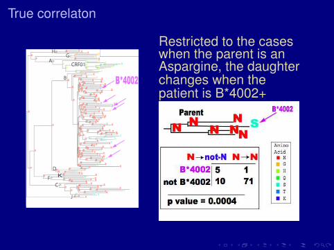
True correlaton

Restricted to the caseswhen the parent is anAspargine, the daughterchanges when thepatient is B*4002+

Sensitivity and Specificity

The new method does correct for the phylogenetic artifact.

Without phylogenetic correction, silent mutations correlate atthe same rate with host HLA.Silent: 10/153 (3–12%)Non-silent: 138/1732 (7–9%)Some silents are very significant: p < 0.00002.

With phylogenetic correction 62/80 significant cases due toclade association, and only 7/80 strongly supported.

4/6 were known epitopes, and 2 more were later experimentallyfound to be true.

Also performs well on synthetic data.

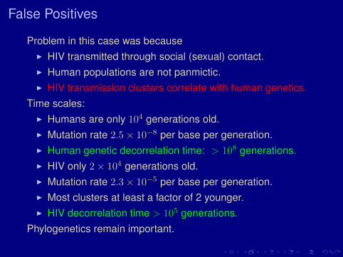
False Positives

Problem in this case was becauseI HIV transmitted through social (sexual) contact.I Human populations are not panmictic.I HIV transmission clusters correlate with human genetics.

Time scales:I Humans are only 104 generations old.I Mutation rate 2.5× 10−8 per base per generation.I Human genetic decorrelation time: > 108 generations.I HIV only 2× 104 generations old.I Mutation rate 2.3× 10−5 per base per generation.I Most clusters at least a factor of 2 younger.I HIV decorrelation time > 105 generations.

Phylogenetics remain important.

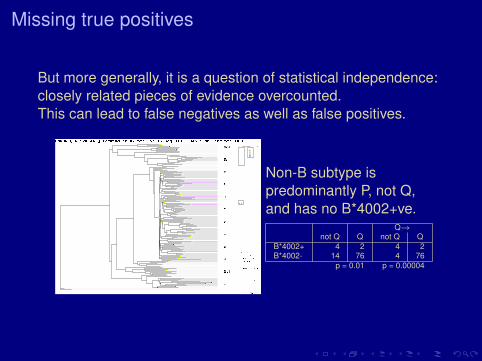
Missing true positives

But more generally, it is a question of statistical independence:closely related pieces of evidence overcounted.This can lead to false negatives as well as false positives.

Non-B subtype ispredominantly P, not Q,and has no B*4002+ve.

Q→not Q Q not Q Q

B*4002+ 4 2 4 2B*4002- 14 76 4 76

p = 0.01 p = 0.00004

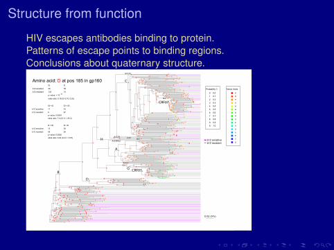
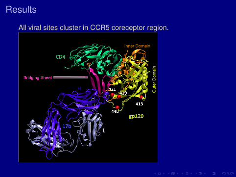
Structure from function

HIV escapes antibodies binding to protein.Patterns of escape points to binding regions.Conclusions about quaternary structure.

60

656

000

00

000

0

00000000

16

000

00

000

00

000

0

00

0

00000

000

00

0000

000

20000

00000

0

0

0

0

00

8

4

4

2

000

11

2

2

1

0011

61

0000

11

1

1

2

8986

6

856

666

6

6X

266

66

6

90

X9999

6

6

6

6

6

6

6

4466

6

9

00000

0

00

000

00

0

000

0

00

0

0

0

0000

0

0

0000

000

111

11

00

0

0

XX

6

7

0000

64

44

19

09

03

00X

XXX

13XX

X

000

X

X

8

9

9

XX

XXXX

XXXX

XXX

X

X

X

X

XXXX

X

88XX

XX

X

X

X

X

X

X

XXXX

XX

5

XXXXX

XXX

X

0

XXXXX

X

XX

X

X

X

XXX

XXXX

XX

0XX

XXX

X

X

XX

XXXXX

XX

X

1XX

X

X

X 000 0X00 0 X00000 X0 0X0000 0000 X00 00 0 00 X0 0 0 00X 00 00 X 000 0 00 0X X0 0 000000 0X 0 000 X0 0000 00X 0 X 00X00 0000 00 000 0X 0 XX000 000 000 X0 000 0 0 X0X0 X 0XX0000X 00 XXX0 00 00 0X 00 0 00 00 00X X 0 0 00X00 0 000 000 00 000 00000 0X0 X 000 00000 00 XX 0 00 0 00 X X00 0 00 0000 00 00 00 00 0 X00 000XX0X X 00X X X 0XXX 0XXX 0 XX X XX XX 0 0 X00 XXX XX 0XXX 000 XX 0X XX 0000 XX XXXX XX0 0X 0 X0XXXX XX 00 0XX 0X0 0X XXX X 0X0X 00XX

Amino acid: D at pos 185 in gp160

38 50

132 31

!D D

b12 sensitive

b12 resistant

SíYDOXH������

odds ratio: 0.18 (CI 0.10, 0.32)

11 25

6 97

�'í!' �'í!�'

b12 sensitive

b12 resistant

SíYDOXH��������

odds ratio: 7.0 (CI 2.1, 25.3)

13 39

35 25

'í!�' 'í!'

b12 sensitive

b12 resistant

SíYDOXH��������

RGGV�UDWLR��������&,�����������

- 8

A/C/D

C

A/C/D

B/CC/D

HA/CRF02

A

A/D

GCRF01

D

B

CRF07

G/J

B/C

Amino Acids

D

N

T

S

R

E

K

H

G

P

V

A

L

F

I

Q

0

1

2

3

�

5

6

7

8

9

X

3UREDELOLW\�D

0.0

0.1

0.2

0.3

���

0.5

0.6

0.7

0.8

0.9

1.0

b12 sensitive

b12 resistant

0.02 (5%)

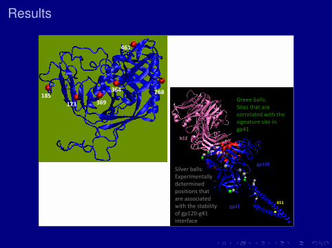
Results

ImmunogenicitySome antibodies neutralize many viruses. Rarely produced.Some people make good antibodies.

Host genetics or viral genetics?

Results

All viral sites cluster in CCR5 coreceptor region.

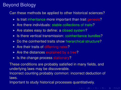
Beyond Biology

Can these methods be applied to other historical sciences?

I Is trait inheritance more important than trait genesis?I Are there individuals: stable collections of traits?I Are states easy to define: a closed system?I Is there vertical transmission: coinheritance bundles?I Do the coinherited traits show hierarchical structure?I Are their traits of differring rates?I Are the distances explained by a tree?I Is the change process stationary?

These conditions are probably satisfied in many fields, andunderlying laws may be discoverable.Incorrect counting probably common: incorrect deduction oflaws.Important to study historical processes quantitatively.