PHYLOGEOGRAPHY OF CRYPTOTIS PARVA IN THE...

PHYLOGEOGRAPHY OF CRYPTOTIS PARVA IN THE UNITED STATES USING

MORPHOMETRICS AND POPULATION GENETICS

Sarah J. Hutchinson

A Thesis Submitted to the

University of North Carolina Wilmington in Partial Fulfillment

of the Requirements for the Degree of

Master of Science

Department of Biology and Marine Biology

University of North Carolina Wilmington

2010

Approved By:

Advisory Committee

Marcel van Tuinen Brian Arbogast

David Webster

Chair

Accepted by

Dean, Graduate School

TABLE OF CONTENTS

ABSTRACT ................................................................................................................................................ iv

ACKNOWLEDGMENTS ............................................................................................................................. v

LIST OF TABLES ....................................................................................................................................... vi

LIST OF FIGURES ..................................................................................................................................... vii

INTRODUCTION ......................................................................................................................................... 1

METHODS.................................................................................................................................................... 6

Morphology ...................................................................................................................................... 6

Genetics ............................................................................................................................................ 9

RESULTS.................................................................................................................................................... 13

Morphology .................................................................................................................................... 13

Genetics .......................................................................................................................................... 21

Cytochrome-b .................................................................................................................... 21

Apolipoprotein and Cytochrome Oxidase I....................................................................... 29

DISCUSSION ............................................................................................................................................. 33

Taxonomy and Systematics ............................................................................................................ 33

Revised Distribution ....................................................................................................................... 36

Phenotypic Plasticity and Bergmann’s Rule .................................................................................. 38

Biogeography ................................................................................................................................. 39

CONCLUSIONS ......................................................................................................................................... 41

Conservation .................................................................................................................................. 41

Future Focus ................................................................................................................................... 42

LITERATURE CITED ............................................................................................................................... 43

APPENDIX I ............................................................................................................................................... 48

APPENDIX II ............................................................................................................................................. 60

iv

ABSTRACT

The least shrew (Cryptotis parva) is a short-tailed shrew (Insectivora: Soricidae) whose

distribution encompasses the central and eastern United States from New Mexico and Wyoming eastward

to the Atlantic coast and northward to Michigan, Southern Ontario, and New York. Traditional taxonomy

recognizes five subspecies of least shrew in the United States: C. p. parva, C. p. harlani, C. p. elasson, C.

p. floridana, and C. p. berlandieri. Most of these taxa, however, were named on the basis of

morphological characters in relatively few specimens, and the validity of some designations has been

questioned. The current study used morphological cranial characters in conjunction with molecular

techniques to do the first thorough revision of the genus in the United States in about 100 years. Seven

cranial measurements were used to perform multivariate statistics on 1020 specimens to elucidate

geographic patterns in morphology. Additionally, three genetic markers (cytochrome-b, barcode, and

Apolipoprotein-B) were used to infer genetic relationships using Bayesian, maximum likelihood, and

maximum parsimony methods. Results indicate that two genetically distinct, sympatric species of least

shrew exist in the United States, Cryptotis parva and Cryptotis floridana, and that both species show

evidence of phenotypic plasticity throughout their ranges. Furthermore, within C. parva there is no

evidence for the validity of C. p. harlani or C. p. elasson.

v

ACKNOWLEDGMENTS

Thank you to my committee my mentors and committee members David Webster, Marcel van

Tuinen, and Brian Arbogast. I also want to acknowledge funding from Figure ‘8’ Beach Homeowners’

Association and UNCW. Special thanks to the curators of the following museums that provided

specimens and tissues, without which this project would not have been possible: American Museum of

Natural History (AMNH), Natural History Museum, Cornell University (CU), Field Museum of Natural

History (FMNH), Georgia Museum of Natural History (GMNH), Highlands Biological Station (HBS),

Illinois Natural History Survey (INHS), Museum of Natural History, University of Kansas (KU),

Louisiana State Museum (LSU), Museum of Comparative Zoology, Harvard University (MCZ), Fort

Hays State University, Sternberg Museum of Natural History (MHP), Museum of Southwestern Biology

(MSB), Museum of Vertebrate Zoology, University of California (MVZ), North Carolina State Museum

of Natural Sciences (NCSM), National Museum of Natural History (NMNH), Royal Ontario Museum

(ROM), Florida Museum of Natural History (FLMNH), Museum of Zoology, University of Michigan

(UMMZ), and Natural History Museum, University of North Carolina Wilmington (UNCW).

vi

LIST OF TABLES

Table Page

1. Definition of cranial characteristics measured on 1020 specimens of Cryptotis parva ................... 7

2. Primers used to amplify mitochondrial and nuclear markers ......................................................... 12

3. Eigenvector loadings on principal components I & II for seven measurements in C. parva ......... 14

vii

LIST OF FIGURES

Figure Page

1. Traditional taxonomic distribution of Cryptotis parva and its subspecies in the United States....... 2

2. Measurements taken from 1020 specimens of Cryptotis parva ....................................................... 8

3. Locations of 67 OTUs in the United States and Mexico ................................................................ 10

4. Principal component analysis for the means of 67 OTUs of Cryptotis parva ................................ 15

5. Phenogram based on a cluster analysis of seven cranial characters ............................................... 17

6. GLS plotted against latitude for 1020 specimens of Cryptotis parva ............................................ 19

7. GLS plotted against longitude for 1020 specimens of Cryptotis parva ......................................... 19

8. Interpolated GLS measurements from 1020 specimens using ArcGIS .......................................... 20

9. Bayesian phylogenetic tree based on a 218 bp fragment of the cytochrome-b .............................. 22

10. Mismatch distribution of all samples for which cytochrome-b was amplified .............................. 25

11. Mismatch distribution frequency for the Floridana Group............................................................. 26

12. Mismatch distribution frequency for the Parva East Population .................................................... 26

13. Mismatch distribution frequency for the Parva West Population .................................................. 26

14. Network analysis of least shrew cytochrome-b sequences............................................................. 28

15. Maximum likelihood tree of a 210 bp fragment of ApoB .............................................................. 30

16. Maximum likelihood tree of a 143 bp fragment of cytochrome oxidase I of the mitochondria .... 32

17. Geographic distribution of molecular sequences overlaid onto the interpolated GLS sizes .......... 35

18. Revised distribution of Cryptotis parva and Cryptotis floridana in the United States .................. 37

PHYLOGEOGRAPHY OF CRYPTOTIS PARVA IN THE UNITED STATES USING

MORPHOMETRICS AND POPULATION GENETICS

INTRODUCTION

Shrews belong to a very speciose family, Soricidae, comprised of over 250 currently recognized

species. Members of this family span Africa, Eurasia, and the Americas. The least shrew, Cryptotis

parva, is a short-tailed, small shrew in the subfamily Soricinae, and is the only shrew to have penetrated

into South America (Churchfield, 1990). It averages about 70-92 mm in total length, with a 13-26 mm

tail, 9-13 mm hind foot, and weighs around 4.0 g (Webster et al., 1985). Its dense, short pelage is

brownish to grayish in color with a paler underside, its tail is bicolored, and its eyes and ears are small.

The pointed snout contains 30 pigmented teeth with bilobed incisors, four unicuspids, and a W-shaped

ectoloph pattern on the fourth premolar and molars. The fourth unicuspid in Cryptotis parva is minute

and usually not visible in a lateral view. This unique dentition distinguishes Cryptotis from other North

American short-tailed shrews (genus Blarina). Finally, as is the case with all shrews, Cryptotis parva

lacks zygomatic arches and auditory bullae (Hall, 1981; Whitaker, 1974).

The least shrew is the only species of Cryptotis in the United States. Its geographic distribution

(Fig. 1) ranges throughout the Southwest eastward to the East Coast, southward to Florida, and northward

to southern Ontario, New York, and Connecticut (Hall, 1981). Newly discovered populations of C. parva

in Wyoming (Marquardt et al., 2006) and New Mexico (Hafner and Shuster, 1996) indicate a recent

westward range expansion. Five subspecies currently are recognized (Merriam, 1895; Hall, 1981;

Whitaker and Hamilton, 1998). The subspecies were first described in the mid-1800s to the mid-1900s

based primarily on cranial and dental characteristics as well as variations in pelage coloration. The

subspecies C. p. parva is found throughout most of the range described above; it is moderate in size. C.

p. floridana, which is the largest subspecies in external and cranial measurements, is restricted to

peninsular Florida and southern parts of Georgia. C. p. berlandieri is similar to C. p. parva in size, but it

has been described as having noticeably larger teeth that vary to a subtle degree in their orientation

2

Fig. 1: Traditional taxonomic distribution of Cryptotis parva and its subspecies in the United States.

(1=C. p. parva, 2=C. p. harlani, 3=C. p. elasson, 4=C. p. floridana, 5=C. p. berlandieri) Map modified

from Hall (1981). Dots represent marginal records; exact locations and citations can be found in Hall &

Kelson (1959) and Hall (1981).

3

(Baird, 1859); it inhabits the Rio Grande Valley southward into northern Mexico. C. p. elasson of Ohio

and C. p. harlani of Indiana and parts of Illinois are smaller than C. p. parva (Bole and Moulthroup,

1942). Prior to these descriptions there was much taxonomic confusion, and, in fact, members of the

genus Cryptotis were included in the genus Blarina (Whitaker, 1974).

Bole and Moulthroup (1942) considered a specimen of Cryptotis harlani from New Harmony,

Indiana, to be an intergrade between C. p. elasson and C. p. parva, noting that, although it was similar in

size to C. p. parva, its pelage was darker with a hint of gray (like that of C. p. elasson). It is noteworthy

that only 12 specimens of C. p. harlani from Illinois and Indiana were examined by Bole and Moulthrop

(1942), and of these, nine were taken from owl pellets, so the skulls could not be compared in their

entirety. Pelage color can be useful in identifying variation in some organisms; however, in most shrew

species this character is highly variable (Choate, 1970). In most parts of the range, least shrews exhibit

seasonal variation in pelage color, displaying a darker hue in the winter than in the summer (Jackson,

1961; Lyon, 1936). Also, juvenile shrews have been reported to be slightly darker than adults (Jackson,

1961), and museum specimens often become foxed and pigmentation changes over time (Lowery, 1974;

Handley and Varn, 1994).

In the last three decades the validity of C. p. harlani has been doubted. In Illinois, C. p. harlani

was thought to occupy the eastern part of the state, whereas C. p. parva was thought to occupy the

western and southern parts of the state. Mumford and Whitaker (1982) declined to differentiate

specimens from Indiana as a separate subspecies other than C. p. parva, claiming more investigation was

needed to clarify the issue. Hoffmeister (2002) performed canonical variate and discriminant function

analyses on five groups of Cryptotis from eastern Nebraska (C. p. parva), western Illinois (C. p. parva),

eastern Illinois (C. p. harlani), southern Illinois (C. p. parva), and western Indiana (C. p. harlani). This

study revealed no significant difference in cranial characteristics between any of these groups. Based on

these results, Hoffmeister (2002) concluded that Cryptotis parva harlani was not a distinct subspecies.

Least shrews from Florida are larger in size when compared to specimens of Cryptotis parva

throughout the remainder of its geographic range, and currently these populations are designated as the

4

subspecies C. p. floridana (Whitaker, 1974; Hall, 1981). There is some question, however, as to exactly

how different least shrews in Florida and parts of southern Georgia are when the species as a whole is

compared on a larger geographic scale, and taxonomic designation has fluctuated between subspecific and

specific levels over the years. Baird (1857) noted obvious differences between an individual from Indian

River, Florida and those from other locations in the geographic distribution of Cryptotis. Whitaker and

Hamilton (1998) agreed with Handley and Varn (1994) that specimens in southeastern Georgia and

Florida are also darker and have longer tails than Cryptotis parva from sites located farther north.

Handley and Varn (1994) agreed with the conclusion of Merriam (1895) that these organisms were

specifically distinct, with specimens from southeastern Georgia and peninsular Florida comprising

Cryptotis floridana.

Large sizes of C. parva have been observed in animals along the Atlantic Coast as well as in

Florida, leading some investigators to believe that the range of C. p. floridana is not restricted solely to

Florida. Handley and Varn (1994) compared samples from southern Florida, northern Florida, coastal

South Carolina, coastal North Carolina, and Raleigh, North Carolina (the latter used to represent typical

C. p. parva in size similar to that at the type locality in Blair, Nebraska). They noted that specimens

demonstrate clinal decreases in size from south to north and that they often appear larger near the coastal

regions of North and South Carolina. In the specimens they examined there was a 10.2% decrease in total

length from southern Florida to coastal North Carolina (indicating that even within Florida organisms are

biggest in the southern part of the state), but from coastal North Carolina to Raleigh (a much shorter

geographic distance) there was a 12.3% decrease in total size. Also, the tail length in specimens from

Florida northward along the coast to North Carolina was 25% of their total length, but those of Raleigh

specimens averaged 21%. These findings led to the conclusion that specimens from coastal North

Carolina and coastal South Carolina represent the same taxon found Florida. This interpretation finds

support from Baird (1857), who first suggested that least shrew specimens from South Carolina

constituted the same population as those in Florida.

5

Preliminary evidence (Hutchinson, 2007) from statistical analyses of cranial characteristics

suggests that specimens of C. parva from the Outer Banks of North Carolina are noticeably and abruptly

larger than those existing on the adjacent mainland in Dare and Hyde counties. The possibility exists that

these specimens may represent an undescribed subspecies or C. p. floridana. Further investigation into

these specimens is warranted to better identify their taxonomic status.

Hall (1981) last provided the distributional limits of the five subspecies of Cryptotis parva, but

his interpretation was based in large part on the revision done by Merriam (1895) almost 100 years

earlier, which was based on morphological characteristics of relatively few specimens. Changes in

morphology are assumed to reflect changes in genetic structure (Avise, 2004), so taxonomy based on

morphology is often useful when delineating genera or species. However, this method alone often falls

short when used to infer population dynamics within a species that may not have had time for the

morphological changes to reflect the molecular changes. Modern molecular techniques can be used in

conjunction with traditional morphometrics to gain a better understanding of the phylogeography of

closely related taxa.

Mitochondrial DNA is useful for studying evolutionary events on the intraspecific level because

of its high rate of evolutionary substitutions and maternal inheritance (Kocher et al., 1989; Avise, 2004).

Cytochrome-b (cyt-b) and cytochrome oxidase I (COI) are two mitochondrial markers that have been

shown to be appropriate for resolving relationships over the last 20 MY and have been widely used to

analyze animal sequences (Harrison, 1989; Irwin et al., 1991; Peppers and Bradley, 2000; Shinohara et

al., 2003; Avise, 2004; Blois and Arbogast, 2006). Nuclear DNA evolves at a much slower rate than

mitochondrial DNA and, therefore, is useful for resolving relationships at higher taxonomic levels. The

Apolipoprotein-B (ApoB) marker from the nuclear genome will be used in conjunction with

mitochondrial DNA to provide multiple lines of evidence for the genetic relationships within Cryptotis of

the United States. The ApoB gene was chosen in this study because of the availability of published

sequences of three species of least shrews, including one sequence of Cryptotis parva.

6

This study will use both morphology and molecular data to infer the phylogenetic relationships of

Cryptotis parva throughout its range in the United States. Specifically, the following null hypotheses will

be tested:

1) Samples of Cryptotis parva parva, Cryptotis parva elasson, Cryptotis parva harlani, Cryptotis

parva floridana, and Cryptotis parva berlandieri are not significantly different from one another

in their morphometrics or genetics.

2) Specimens along the East Coast of the United States are not significantly larger than those further

inland.

3) The population of Cryptotis parva on the Outer Banks of North Carolina is not distinct from those

on the adjacent mainland in their morphometrics or genetics.

METHODS

Morphology

A total of 1700 specimens of Cryptotis parva from 18 museums were examined for

morphological analysis (Appendix I). Materials examined from these specimens included combinations

of skins, skulls, and complete skeletons. External measurements (total length, tail length, hind foot

length, and weight) as well as any additional information were recorded from specimen tags.

Furthermore, seven cranial measurements were taken with digital calipers to the nearest 0.1 mm from

individuals (n=1020) whose condition allowed for the complete suite of measurements to be taken. These

measurements included: greatest length of skull (GLS), occipital-premaxillary length (OPL), interorbital

breadth (IB), greatest cranial breadth (GCB), width across molars (WM), palatine length (PL), and the

distance from the fourth premolar to third molar (P4-M3). These measurements were selected because

they have proved useful in determining shrew relationships by other investigators (Bole and Moulthrop,

1942; Choate, 1970; Genoways and Choate, 1972; Moncrief et al., 1982; Woodman and Timm, 2000).

For definitions of measurements see Table 1 and Fig. 2.

7

Table 1: Definition of cranial characteristics measured on 1020 specimens of Cryptotis parva. The

numbers correlate with those in Figure 2.

Number Abbreviation Measurement Definition

1. GLS Greatest Length of Skull Greatest distance from the posterior-most

projection of the occipital to the anterior-

most projection of the upper incisors

2. OPL Occipital-Premaxillary

Length

Distance from the posterior-most

projection of the exoccipital condyle to the

anterior-most projection of the premaxillae

3. IB Interorbital Breadth Least distance across the orbits measured

perpendicular to the longitudinal axis of the

cranium

4. GCB Greatest Cranial Breadth Greatest mastoidal breadth measured

perpendicular to the longitudinal axis of the

cranium

5. WM Width Across Molars Greatest distance across the palate

between the labial-most projections of the

upper molars

6. PL Palatal Length Greatest distance from the anterior-most

point of the upper incisors to the hind edge

of the bony palate

7. P4-M3 Fourth Premolar to Third

Molar Length

Greatest distance from the anterior-most

projection of the upper premolar to the

posterior-most projection of the upper

third molar

8

Fig. 2: Measurements taken from 1020 specimens of Cryptotis parva. The numbers correlate with the

definitions given in Table 1. (Image modified from Whitaker, 1974)

9

Because external measurements were taken by many individuals, and are therefore highly

variable, only cranial measurements taken personally were used in statistical analyses. Individuals whose

cranial sutures were not fused were considered to be juveniles and were excluded from analyses.

Individuals for which cranial measurements were able to be taken were grouped into 67 operational

taxonomic units (OTUs) based on geographic location, being careful not to cross any current taxonomic

designations, major physiographic provinces, or major geographic boundaries (Fig. 3).

A single classification analysis of variance (F-test, significance level 0.05) was used to test for

significant geographic variation among the OTUs using the GLM procedure in SAS (v9.1), and a Tukey’s

HSD posteriori pairwise test was used to determine which OTUs differed significantly. Principal

components analysis was performed by deriving a product-moment correlation matrix from variance-

standardized character means for each OTU, extracting eigenvectors, and generating a two dimension plot

of OTUs. Additionally, the MEANS, CLUSTER, and TREE procedures were used in SAS (v9.1) to

generate means for each measurement of each OTU, cluster the means hierarchically, and create a

phenogram based on the clusters, respectively. Finally, coordinates for each individual were acquired

from the MANIS database, when possible, or interpreted from Google Earth (v5.1) for analyses of clinal

variation using standard correlation and regression calculations derived from Excel between cranial size

and latitude and longitude. Furthermore, the coordinates were put into ArcGIS (v9.3.1) to interpolate

measurements for parts of the range where specimens were either not available or too badly damaged to

measure.

Genetics

Fresh tissue samples were obtained from New Hanover and Brunswick counties of North

Carolina (n=3), frozen tissue collections at the Natural History Museum at UNCW (n=7), and loan

requests made to frozen tissue banks around the country (n=10). However, these individuals neither

encompassed the scope of the distribution of Cryptotis parva in the United States, nor allowed for

10

Fig. 3: Locations of 67 OTUs in the United States and Mexico.

11

extensive sample size. Fresh tissues were supplemented using toes from prepared specimens at the

UNCW Natural History Museum (n=13) and using soft tissue that remained on museum skulls after the

cleaning process was complete, referred to as residual tissue (n=46). Finally, 11 sequences were obtained

from the GenBank database, including outgroup sequences of Blarina brevicauda, B. carolinensis, C.

magna, C. goldmani, and C. mexicana for cytochrome-b and C. magna and C. goldmani for ApoB. A

complete list of source museums, tissue type, markers amplified, and collection locations are in Appendix

II.

Tissues were extracted according to the protocol of the Animal Extraction Kit from MOBIO

Laboratories (Carlsbad, CA). Following extraction, PCR inhibitors were removed using the MOBIO

PowerClean Kit.

A 218 bp fragment of cytochrome-b was amplified for 79 individuals using primers 950F/15915,

950F/1118R, 1021F/15915 (Irwin et al., 1991). A 143 bp fragment of cytochrome oxidase I was

amplified for 21 fresh tissue extractions using primers COIF/COIR, and a 210 bp fragment of

Apolipoprotein-B was amplified for 14 fresh tissue extractions using ApoF/ApoR (Table 2). Due to the

low success rate for COI and ApoB, these markers were used only to corroborate any patterns observed in

the cyt-b data. PCR amplification was performed following the protocol of GoTaq Green Master Mix

from Promega Corp. (Madison, WI). Thermocycler conditions were set at 40 cycles of 95ºC for 2min,

95ºC for 50s, 50ºC for 50s, and 72ºC for 40s, with an extension at 72ºC for 5min at the end of the PCR.

PCR products were first visualized on a 2% agarose gel electrophoresed for 20min and soaked in

ethidium bromide for 15min. Products were then purified according to the ExoSAP protocol from USB

Corporation (Cleveland, OH) before final sequencing was outsourced to Macrogen Inc. (Seoul, Korea).

Sequences were aligned with Sequencher 4.8 and refined by eye, and the possibility of pseudogenes in the

dataset was rejected by the lack of stop codons and the presence of expected proportions of bases in the

sequences (i.e. low GC content in mitochondrial DNA).

12

To apply the appropriate substitution model to the alignment of the three markers, JModelTest

version 0.1.1 (Guindon and Gascuel, 2003; Posada, 2008.) was used. This software analyzes 88

nucleotide substitution models of increasing complexity and uses a likelihood ratio test based on the AIC

Table 2: Primers used to amplify mitochondrial and nuclear markers.

Primer Sequence (5´-3´)

950F TCYAAACAACGAAGYATAATA

1021F AGGACARCCCGTCGAACAYCC

1118R TCRARTAGGCTTGTGATTGG

COIF CCGYTGAYTATTYTCTACYAACCAC

COIR GAAAATTATRACRAATGCGTGRGC

ApoF TGAGAAAGTCAGAGACCAGGC

ApoR ACAGAGAAGCCAGAACCCAGG

criterion to find the best-fit model, including appropriate gamma distributions for modeling rate

heterogeneity across sites and percentage of invariant sites for modeling the unchanging portion of the

data. The hypothesis of recent population growth was tested using Tajima’s D, Fu’s Fs, and mismatch

distribution tests in Arlequin v3.1 (Excoffier et al., 2005) using the appropriate gamma and base

frequencies obtained from jModelTest. Additionally, genetic diversity indices of Theta-pi and Theta-S

were obtained. Analysis of Molecular Variance (AMOVA) was run based on the genetic structure

obtained from phylogenetic analyses, using clades that grouped together with posterior and bootstrap

probabilities greater than 50%. Haplotype genealogies were estimated using minimum spanning network

analyses in TCS version 1.21 (Clement et al., 2000), which calculates the level of divergence for

connections that have a maximum parsimony probability greater than 0.95 (Templeton et al., 1992).

Inference of phylogeny was done using Bayesian methods for the cytochrome-b marker in

BEAST v1.4.8 and its accompanied program Tree Annotator v1.5.3. Bayesian analyses use

13

predetermined priors to search the set of trees with the best topologies and combination of parameters

(Felsenstein, 2004). For this study, all priors were left at the default values except for clock calibrations.

Assigning Blarina brevicauda and Blarina carolinensis as a monophyletic outgroup, the lower and upper

bounds of the split between Cryptotis and Blarina were set at 9 MYA and 15 MYA, respectively, based

on the ages of the oldest modern Cryptotis fossil and the oldest Adeloblarina fossil (Harris, 1998).

Cryptotis goldmani, C. mexicana, and C. magna were also assigned to be included in order to better

calibrate the bounds. Three independent MCMC analyses were run for 80 million iterations with a burn-

in of 10%. Each analysis was viewed using Tracer v1.4, appropriate ESS values were verified (>200),

and convergence between runs was checked. The three analyses were then combined to create one

uniform tree using Tree Annotator v1.5.3, and the tree was viewed and formatted using FigTree v1.3.

PAUP* version 4.0 (Swofford, 2003) was used to calculate bootstrap values using 1000 replicates,

likelihood optimality criterion, neighbor-joining search method, and the best-fit model results from

jModelTest. These values were then superimposed onto the Bayesian gene tree created for cytochrome-b.

Maximum likelihood trees were generated in PAUP* for the nuclear Apolipoprotein-B and the

mitochondrial COI genes according to the parameters determined in jModelTest. Additionally, bootstrap

values were generated for both markers using both likelihood and parsimony optimality criteria.

RESULTS

Morphology

Ninety percent of the variation among the 67 OTUs is accounted for on the first two principal

components (Table 3). Principal component I (PC I) explains 83% and principal component II (PC II)

explains 7% of the overall variation in the data set. All seven cranial characteristics load positive on PC I

and have approximately the same loadings (Table 3). Therefore, PC I reflects size. Only interorbital

breadth (IB) and greatest cranial breadth (GCB) load positively on PC II and eigenvector loadings

indicate that IB, GCB, and palatal length (PL) have the most influence, with the latter loading negatively.

Therefore PC II represents shape, indicating an inverse trend between cranial and interorbital width on

14

one hand and palatal length on the other along this factor. Width across molars (WM) also loads

negatively on PC II, indicating that more robust animals do not necessarily become more robust in

toothrow characteristics.

Table 3: Eigenvector loadings on

principal components I & II for

seven measurements in C. parva.

Variable PCI PCII

GLS 0.41 -0.09

OPL 0.40 -0.07

IB 0.35 0.58

GCB 0.35 0.55

WM 0.37 -0.11

PL 0.37 -0.51

P4_M3 0.39 -0.26

Total variation explained (%)

83 7

When PCI and PC II are plotted against one another (Fig. 4), four groups of OTUs are revealed.

A general pattern of increasing size from inland populations to coastal populations, with the largest

individuals residing in Florida, is apparent. Group I has the most negative PC I values. This group

includes OTUs from the remainder of the species range. This group is formed from inland OTUs with

only two exceptions, OTU 46 from New Hanover County, North Carolina and OTU 41 from Hyde

County, North Carolina.

Group II is made up of only three OTUS (8, 10, and 49) from the general areas of Logan County,

Arkansas, Aransas County, Texas, and Aiken County, South Carolina. Least shrews from these OTUs are

moderate in overall size (PC I), but they have negative values on PC II and are characterized by having

narrow cranial and interorbital regions but relatively long palates. No geographic coordination between

these groups is apparent, however.

Group III is primarily formed from coastal OTUs (13, 33, 34, 42, 43, 50, 55, and 57) as well as

two OTUs in Florida (63 and 65). These OTUs are smaller than those in Group IV in overall size (PC I)

and they have less variation in shape (PC II). The largest group (Group IV) consists of eight OTUs from

15

Fig. 4: Principal component analysis for the means of 67 OTUs of Cryptotis parva. Principal Component

I (Prin1) represents overall size and Principal Component II (Prin2) represents an inverse relationship

between interorbital and cranial breadth on one hand and palatal length on the other.

16

Florida (OTUs 58, 59, 60, 61, 62, 64, 66, and 67) as well as OTU 28 from New Jersey, OTU 11 from

Hidalgo County, Texas, and OTU 53 from Liberty County, Georgia, which are all coastal locations.

These OTUs are strongly positive on PC I, but their PC II loadings range from strongly positive (OTU 67,

Key Largo, Florida) to strongly negative (OTU 61, St. Johns County, Florida), indicating large variation

in cranial robustness and palatal length.

It is important to note that the group assemblages produced by this PCA do not correlate

geographically with the distributions of C. p. elasson or C. p. harlani whose type localities are included in

OTU 26 and OTU 19, respectively. OTU 19 is neither unique along PC I or PC II which coincides with

the results found by Hoffmeister (2002). Also, the type locality for C. p. berlandieri (OTU 12) is nested

well within Group I, and does not appear unique according to this analysis. OTU 26 is not unique with

respect to Group I along PC I, but it is the most negative from that group along PC II. However, it is not

the most negative given data from other groups, meaning that while individuals in this area may be on the

slender side, they are not the most slender individuals when considering the entire range under

investigation. OTUs 42 and 43 represent individuals from the Outer Banks, North Carolina and the

adjacent mainland in Dare County, North Carolina. Both fall out within in Group III on the positive side

on the PC I axis.

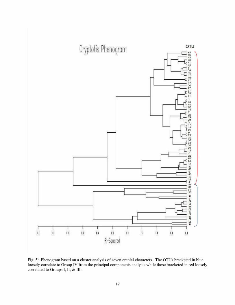
A phenogram (Fig. 5) created using the seven cranial characteristics analyzed supports the trend

seen in the principal components analysis. Two major clades are apparent in the phenogram, which

loosely correspond to Group IV and Groups I, II, and III in the PCA. Although there are a few exceptions

such as OTUs 52, 55, and 8, which include individuals around the areas of Burke and Ben Hill counties in

Georgia and Logan County in Arkansas, the biggest animals group together into a clade consisting

exclusively of OTUs from Florida and other coastal regions. OTUs 18-21 represent individuals of C. p.

harlani from Indiana and Illinois, and OTUs 24, 26, and 27 represent individuals of C. p. elasson. Note

that these OTUs do not group together in any notable pattern.

All seven variables measured display significant (p<0.0001) geographic variation. The

subsequent posterior test (data available from author upon request) revealed that GLS and OPL exhibit

17

Fig. 5: Phenogram based on a cluster analysis of seven cranial characters. The OTUs bracketed in blue

loosely correlate to Group IV from the principal components analysis while those bracketed in red loosely

correlated to Groups I, II, & III.

18

the same pattern. Generally speaking, OTUs in Florida, Texas, and along the Atlantic Coast were not

significantly different from one another, but were significantly different from those in the remainder of

the range. There was no apparent geographic signal in IB or GCB except in extreme parts of the range

(northwest and southern Florida). Relatively few significant differences were evident in WM, PL, and the

distance from the fourth premolar to the third molar (P4-M3) measurements, and those OTUs that were

significant in these variables showed little geographic pattern. Rather, patches of larger and smaller

individuals reside more or less randomly throughout the range. However, even when there is a pocket of

smaller individuals, for example, the difference is clinal. In all measurements OTUs in Florida were

largest. In no measurement were specimens from the type locality of C. p. elasson (OTU 26) and those

from the type locality of C. p. harlani (OTU 19) significantly different from one another. For

comparative purposes C. p. berlandieri is represented by specimens from Tamaulipas, Mexico (OTU 12),

the type locality. These specimens were significantly smaller than those from OTUs 67 (GLS, OPL, and

GCB), 66 (GLS and OPL), 64 (GLS and OPL), 62 (GLS and GCB), and 60, 59, 58, and 28 (GLS), but not

significantly different from C. p. parva in Texas or elsewhere in its range. OTU 16 (Cheatham County,

Tennessee) and OTU 27 (representing Lake County, Ohio, which is an area near the individual used for

molecular analyses from Portage County, Ohio) were both similar to specimens from Florida (OTUs 58,

59, 60, 62, 64, and 67) and New Jersey (OTU 28) and significantly different from all other OTUs in the

measurement of GLS. However, while they were not significantly different from Florida samples, they

were smaller by an average of 1.45 mm (OTU 16) and 1.67 mm (OTU 27). No other geographic variation

was present in any other measurements for these two OTUS except for OPL and GCB where they were

only different from the largest of the samples (Dade Co. and Key Largo, Fl and New Jersey).

Furthermore, specimens from OTU 42 (mainland of Dare County, North Carolina) and OTU 43 (Outer

Banks of Dare County, North Carolina) were not significantly different from one another in any

measurement.

To further investigate whether larger sized shrews in Florida and along the coast were a result of

an abrupt increase or a clinal increase in response to geography, size was plotted against latitude and

19

Fig. 6: GLS plotted against latitude for 1020 specimens of Cryptotis parva.

Fig. 7: GLS plotted against longitude for 1020 specimens of Cryptotis parva.

20

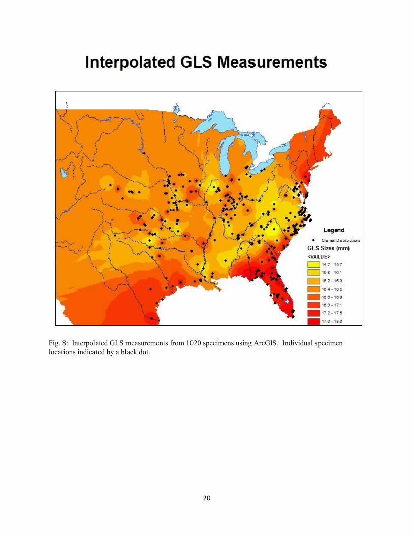
Fig. 8: Interpolated GLS measurements from 1020 specimens using ArcGIS. Individual specimen

locations indicated by a black dot.

21

longitude and correlation analyses were performed (Fig. 6 and Fig. 7). Cranial sizes for the entire species

range were also interpolated in ArcMap version 9.3.1 (ESRI Inc.) using the spatial analyst tool, the

inverse distance weighted method, and the cranial sizes of the 1020 individuals measured (Fig. 8).

Because GLS was determined to express the most variation in the ANOVA, it was used as a proxy for

overall cranial size in these analyses. There is a significant negative correlation (-0.41, p<0.0001)

between latitude and GLS, however the R2 value is only 0.165. Most of this correlation lies between the

latitudes of 25º and 30º which roughly correspond to the latitudes of Florida and southern Georgia.

There is no significant correlation between longitude and GLS (p=0.07). In the scatterplot, however,

increased sizes around the longitudes that correspond with the East Coast are apparent. These results

indicate that Cryptotis does exhibit an abrupt increase in size in the southern parts of its range. The map

of interpolated distances nicely displays the results found in the morphological analyses. Using the

inverse distance weighted method cells without data are assigned values based on cells with data. The

program assumes closer cells should be weighted heavier than cells further away. One caveat of the

method, however, is that it is sensitive to cells with only one data point represented and displays them

with a tight circle of color. Also, the model interpolates for the entire area in question so the color

gradient extends beyond the bounds of the species range.

Genetics

Cytochrome-b

Amplification of the cytochrome-b fragment successfully yielded clean sequences for 79

Cryptotis parva samples: 20 fresh samples, 13 toe tissue samples, and 46 samples of residual cranial

tissue, spanning the species range in the United States (Appendix II). The best fit model of nucleotide

substitution according to the AIC criterion was TIM1+G. This model was used for all analyses in PAUP*

software (Swofford, 2003), however, it is not available in BEAST software and for that reason the second

best model of HKY+G was used to construct a phylogeny of cytochrome-b. Data was partitioned by

22

Fig. 9: Bayesian phylogenetic tree based on a 218 bp fragment of the cytochrome-b. Fifty percent

consensus tree created from the results of three runs that concurrently estimated phylogeny, mutation

parameters, and branch lengths. Time scale is in million years before present. Red indicates the

Floridana Group and blue and green branches are part of the Parva Group. Green branches indicate the

Parva East population and blue branches indicate the Parva West population. Posterior probabilities of

>0.50 are displayed above branches and bootstrap probabilities >50% are displayed below. If a branch

does not have bootstrap support, values are replaced with dashes. The black lines are the individuals from

St. Johns County, Florida and Taylor County, Florida that are loosely referred to as the Parva South

Population.

23

codon position and a Yule Speciation event was determined to have the lowest posteriors and highest

Bayes factors. Bootstrap values were obtained using the distance criterion and a neighbor-joining search

method. To calculate bootstrap values using PAUP* (Swofford, 2003) the following parameters of the

optimized model (T1M1+G) were used: alpha=0.189, A=0.34, C=0.27, G=0.11 and T=0.28.

Four clades emerge in the resulting cytochrome-b gene tree of Cryptotis parva (Fig. 9), which do

not support the traditional systematic distinctions of C. p. parva, C. p. elasson, C. p. harlani, and C. p.

floridana. Most major clades described in the tree are strongly supported by posterior probabilities >0.90

and bootstrap values >50%. The first of these clades (referred to herein as Floridana Group) to emerge

(6.1 MYA) consists of three individuals from Highlands County, Florida, two individuals from Cheatham

County, Tennessee, and one individual each from Thomas, Charlton, and Grady counties in Georgia as

well as Portage County, Ohio and Taylor County, Florida. Bayesian and bootstrap support is strong

(posterior probability=1.0, bootstrap=66) for the monophyly of the Floridana Group to the exclusion of

the remainder of the individuals sampled (referred to as the Parva Group). Structuring within the

Floridana Group began around 3.0 MYA, producing one clade beginning with individuals from Charlton

and Thomas counties in Georgia (posterior probability=0.95) and a second clade comprised of the

remaining specimens (posterior probability=1; bootstrap=92). Structure within the Parva Group began

around 3.4 MYA when three clades emerge. The first radiation to occur within the Parva Group forms

what will be referred to as the Parva West Population which consists primarily of individuals from the

western United States (Arkansas, Louisiana, Kansas, Missouri, Texas, Nebraska, and Indiana) with the

exception of five individuals from Ohio, Maryland, Georgia, and Florida. Bayesian support is strong

(posterior probability=1.0) and there is relatively high bootstrap support (85%) for the monophyly of the

Parva West Population. The next radiation within the Parva Group occurred approximately 3.0 MYA and

produced two clades. This node, however, has neither Bayesian nor bootstrap support. This is due to the

instability of the first clade to emerge consisting of only two individuals, one from St. Johns County,

Florida and one from Taylor County, Florida. Uncertainty exists if these two individuals should form

their own clade (Parva South Population) or belong to the Parva East Population. The last clade to

24

emerge from the Parva Group will be referred to as the Parva East Population, which primarily contains

individuals from the eastern United States (Maryland, North Carolina, West Virginia, Virginia, New

York, and Ohio) except for four individuals from Arkansas, Florida, Oklahoma, and Georgia. The

monophyly of the Parva East and Parva West Populations is strongly supported with posterior

probabilities of 0.92 and 0.99, respectively; however, bootstrap support is weak for both clades.

Structuring within these two clades began roughly 1.3 MYA (Parva West) and 2.1 MYA (Parva East), but

no definitive geographic patterns emerge. Support for terminal nodes of both the Parva Group and the

Floridana Group are lacking, indicating quick population growth and expansion. The nucleotide

substitution rate in this analysis was 0.89subs/site/MY. This rate seems low when considering the high

metabolic rate of least shrews, but it is consistent with data found in other studies (Fumagalli et al., 1999;

Brant and Ortí, 2002).

To further investigate population dynamics, the data was initially analyzed without predetermined

population structure. A mismatch distribution was performed on the traditional C. parva (Fig. 10) which

showed three major peaks and possibly a fourth smaller peak, indicating that the data set represents

multiple populations. Subsequently, structure was enforced in the analyses performed based on the three

main clades (Floridana Group, Parva West, and Parva East) determined in the Bayesian phylogeny. The

individuals from St. Johns and Taylor counties, in Florida, were excluded from these analyses due to the

small sample size and low support of the clade. Phylogenetically, neither individual clearly was placed

among the other well-defined clades. The clade representing Charlton and Thomas counties in Georgia

may represent a unique population within the Floridana Group; however, because of small sample size

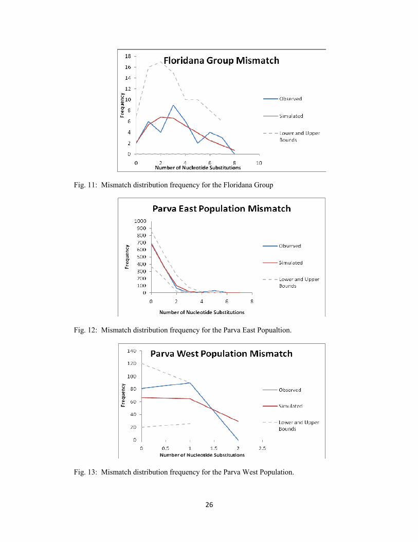
these individuals were analyzed together with the rest of the Floridana Group. Mismatch distributions

performed according to the structure recognized in the Bayesian analysis (Fig. 11-13) show signals of

expansion in each group and population. Fu’s Fs and Tajima’s D values significantly support expansion

in Parva West and Parva East populations. For both populations Fu’s Fs is largely negative and highly

significant (p<0.0001). Tajima’s D is significantly negative (-1.37, p<0.0001) for Parva East, but is not

significant for Parva West (1.54, p<0.524). The mismatch distribution of the Floridana Group either

25

Fig. 10: Mismatch distribution of all samples for which cytochrome-b was amplified. Also shown are

simulated values under constant size (red), including the 5% and 95% bounds.

26

Fig. 11: Mismatch distribution frequency for the Floridana Group

Fig. 12: Mismatch distribution frequency for the Parva East Popualtion.

Fig. 13: Mismatch distribution frequency for the Parva West Population.

27

represents a single expansion that is not sampled efficiently to display a smooth peak, or represents three

peaks. Also, some conflict exists in the Fu’s Fs and Tajima’s D values for this group. Tajima’s D value

for this group indicates significant contraction in the Floridana Group (0.03, p<0.015) while Fu’s Fs

strongly indicates expansion (-6.46, p<0.0001). It is possible that the conflict in this group may indicate

additional structure within the Floridana Group.

AMOVA results supported the separation of the Floridana Group from that of the Parva Group as

well as the separation of the Parva West Population from the Parva East Population. Variation among

groups (Floridana Group and Parva Group) accounted for 76.35% of the total variation in the data set.

The variation among populations within groups (Parva West Population and Parva East Population)

accounted for 19.81% of the total variation. Only 3.83% of the variation was explained by the

relationships within populations. Theta-S (1.35, 0.29) and Theta-pi (0.63, 0.53) diversity indices for the

Parva East and Parva West populations, respectively, indicate slightly more diversity in Parva East. The

most diversity, however, is found in the Floridana Group (Theta-S = 3.31, Theta-pi = 3.33).

When these data are compared to those from a network analysis (Fig. 14) it is clear that these

expansions correlate to what was identified in the phylogeny as the Floridana Group, followed by the

Parva West Population and Parva East Population. The results of the network analysis show that

haplotypes connected by fewer than five nucleotide substitutions are connected with a parsimony value of

>0.95. All cytochrome-b haplotypes were connected in one network. Network analysis considers the

most frequent haplotype to be the oldest and is indicated by a rectangle. Haplotypes are connected by

lines in the genealogy and the open circles between the lines represent missing haplotypes that are either

locally extinct or unsampled in the analysis. The deepest structure in this analysis is apparent in

distinguishing the Floridana Group (red circles) from other haplotypes, followed by separating the Parva

West (green circles) from Parva East haplotypes (blue circles). Consistent with the mismatch distribution,

the Parva East haplotypes display a fairly recent expansion with haplotypes generally one substitution

removed from the most frequent haplotype. The gray circle represents the two individuals from St. Johns

28

Fig. 14: Network analysis of least shrew cytochrome-b sequences. Rectangle indicates the oldest, most

frequent haplotype, and sizes of circles indicate frequency of haplotype. Open circles indicate missing

haplotypes. Colors correspond to clades described in Bayesian analysis: Red = Floridana Group, Green

= Parva West, Blue=Parva East, Grey=Parva South.

29

and Taylor counties in Florida that grouped at the base of the Parva East clade in the phylogeny, but with

little statistical support. In agreement with the Bayesian and ML analyses, these individuals identify more

closely with the Parva East group (separated by fewer missing haplotypes). Network analyses indicate

that this haplotype bridges the three clades, a pattern not observed from phylogenetic analysis.

Apolipoprotein and Cytochrome Oxidase I

The GTR model was used with base frequencies of: A=0.38, C=0.20, G=0.13, T=0.29, acquired

from jModelTest, to generate a maximum likelihood gene tree (Fig. 15) for a 210 bp fragment of

Apolipoprotein-B for 14 Cryptotis parva, one Cryptotis magna, one Cryptotis goldmani, and one Blarina

brevicauda assigned as outgroup (Appendix II). A full heuristic search with TBR branch swapping was

performed to generate the tree. A heuristic search was also used to generate bootstrap values from 1000

replicates using the likelihood criterion, and a fast-heuristic search of 1000 replicates generated the

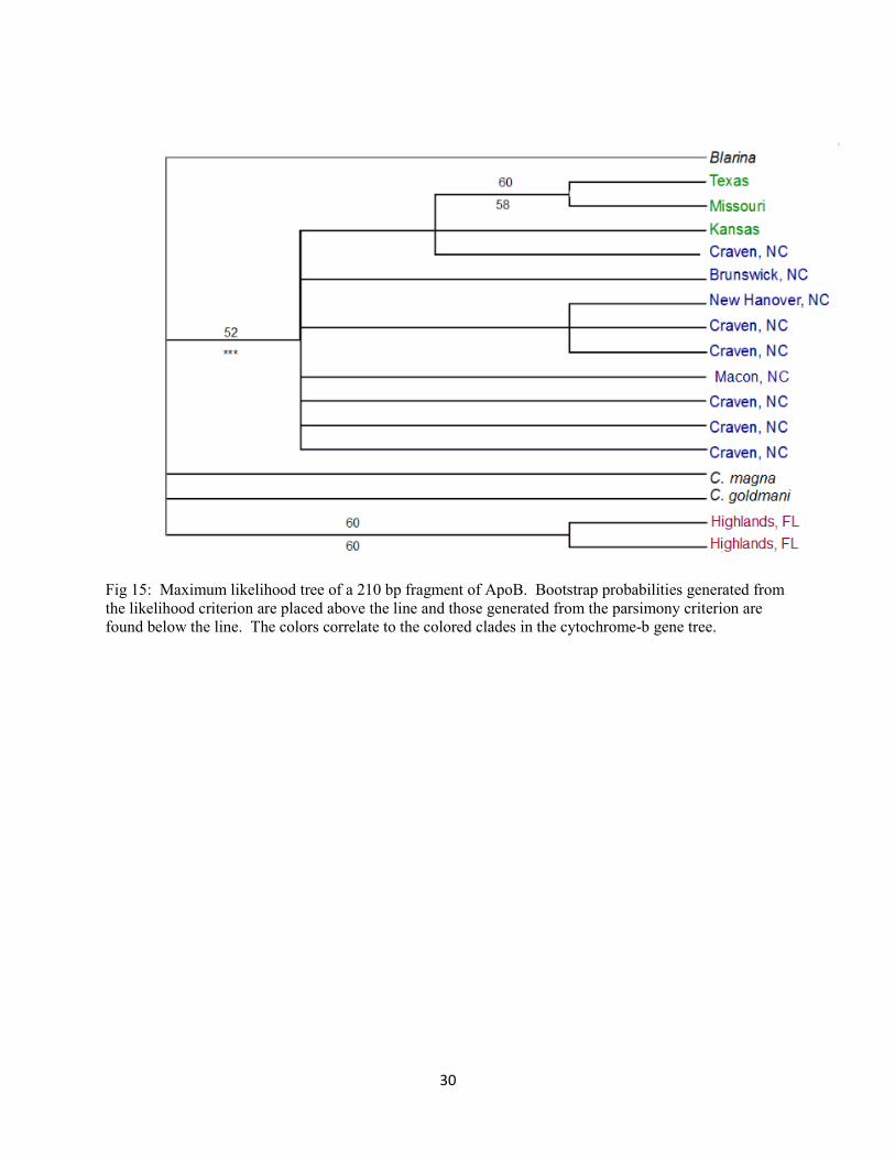
bootstrap values according to the parsimony criterion. Two individuals from Highlands County, Florida

group together to the exclusion of all other Cryptotis with bootstrap value of 60 for both likelihood and

parsimony criterion. The remainder of the Cryptotis sampled from the United States generated a

likelihood bootstrap probability of 52; there is no reportable parsimony value. Finally, an individual from

Tom Green County, Texas (Genbank) and an individual sequenced from Missouri are grouped together

with likelihood and parsimony bootstrap values of 60 and 58, respectively. The only difference between

the ML tree shown and one generated from MP is that the individual from Craven County, North Carolina

does not fall out with the individuals from western states as it does here. Although bootstrap values are

low and there is high amount of polytomy in this gene tree, the general structure seen in the cytochrome-b

data is reflected in the Apolipoprotein-B data as well. The colors of the terminal labels in Fig. 15

correspond to the clades from which these individuals were found in the cytochrome-b data. The two

individuals from Florida clearly represent a group of their own. Also, the same general pattern of an

eastern and western clade of Cryptotis, with the western clade originating from the eastern clade, is seen

in the nuclear data. The discrepancy of the placement of one individual from Craven County, NC could

30

Fig 15: Maximum likelihood tree of a 210 bp fragment of ApoB. Bootstrap probabilities generated from

the likelihood criterion are placed above the line and those generated from the parsimony criterion are

found below the line. The colors correlate to the colored clades in the cytochrome-b gene tree.

31

be explained by the slower rate of evolution in the nuclear genome compared to that of mitochondrial

genome or to differential lineage sorting (Avise, 2004).

The K80 (K2P) model with a gamma value of 0.07 and ti/tv=8.61 was used to create a maximum

likelihood tree for a 143 bp fragment of the mitochondrial COI gene for 20 individuals of Cryptotis parva

(Fig. 16). A full heuristic search with TBR branch swapping was performed to generate the ML tree.

Also, bootstrap values were generated using fast-heuristic searches for both likelihood and parsimony

criteria at 1000 replicates. Unfortunately, at the time of this publication there were no published barcode

sequences for any short-tailed shrews. Furthermore, alignment was unsuccessful using the barcode

sequences published for Crocidura and Sorex specimens. For that reason, the maximum likelihood tree

described is midpoint rooted. Amplification of the barcode in specimens representing the Floridana

Group was also unsuccessful. Nonetheless, the phylogeny and bootstrap values offer strong support for

the structure of the Parva East and the Parva West Populations, although there is overlap between these

groups. Most of the North Carolina specimens grouped together with bootstrap values of 98 (likelihood)

and 72 (parsimony). Contrary to expectations, however, one specimen from Brunswick County does fall

outside of this group, and one specimen from Wabaunsee, Kansas (which would be expected to fall within

the Parva West population) falls within the Parva East population. There is no bootstrap support for the

placement of the specimen from Brunswick County, however, indicating that this sample needs to be

confirmed (which could not be done) or Brunswick County needs to be better sampled.

32

Fig. 16: Maximum likelihood tree of a 143 bp fragment of the cytochrome oxidase I of the mitochondria.

Bootstrap probabilities generated from the likelihood criterion are placed above the line and those

generated from the parsimony criterion are found below the line. The colors correlate to the colored

clades in the cytochrome-b gene tree.

33

Discussion

Taxonomy and Systematics

Neither molecular nor morphological analyses support subspecific designation of Cryptotis parva

elasson in Ohio. In the cytochrome-b phylogeny a sample from northern Ohio groups with the Floridana

Group while two others, one of which is from the type locality of C. p. elasson, groups with the Parva

group. In neither group do these individuals break off into their own clade. In fact, in the Parva Group

the two samples from Ohio are not even assigned to the same population. Morphologically, all OTUs

representing Ohio samples are statistically small in size when compared with samples from Florida and

other coastal areas, whether they genetically fall into the Floridana Group or the Parva Group. However,

for the most part they are not statistically significantly different from other Cryptotis in surrounding

states.

The case is the same with regards to Cryptotis parva harlani. The individual genetically analyzed

was assigned to the same clade as others from Ohio within the Parva Group. Admittedly this race was not

well represented in the molecular analysis. However, in the morphological analyses C. p. harlani was

represented by three separate areas of Indiana (OTUs 11, 12, and 54), one of which includes the type

locality for the subspecies, as well as one area of Illinois (OTU 53). These results agree with those of

Hoffmeister (2002) showing that specimens from Indiana are the same morphologically as specimens

from Ohio. Furthermore, the null hypotheses (specimens from Ohio and Indiana are not significantly

different from one another nor from other Cryptotis parva) could not be rejected. Therefore, there is no

validity to the distinct taxonomic status traditionally given to specimens of Cryptotis in these regions and

both should be referred to as Cryptotis parva parva.

Cryptotis parva berlandieri was represented in the morphological aspect of this study by two

OTUs (11 and 12). Neither principal components analysis nor analysis of variance supported the

subspecific designation given to these individuals, as one would expect if the designation were valid. It

would appear, based on these data, that the individuals collected from these locations are actually

members of C. p. parva. These results coincide with the findings of Raun (1965) who found there was

34

just as much variation in cranial characters within C. p. parva in Texas as between C. p. parva and C. p.

berlandieri. It is possible that C. p. berlandieri does not rightfully exist, or that the distribution line of the

subspecies actually exists somewhere further south in Mexico and that the individuals sampled are

integrades between the two subspecies. Unfortunately lack of sampling within what is currently

recognized as C. p. berlandieri, small sample size (n=1) for OTU 11, and lack of molecular data make

determination of taxonomic status with any reasonable amount of certainty impossible. For this reason,

the null hypothesis that the subspecies C. p. berlandieri is not significantly different from C. p. parva

cannot be supported or rejected and the traditional status of this shrew should be maintained until more

data become available.

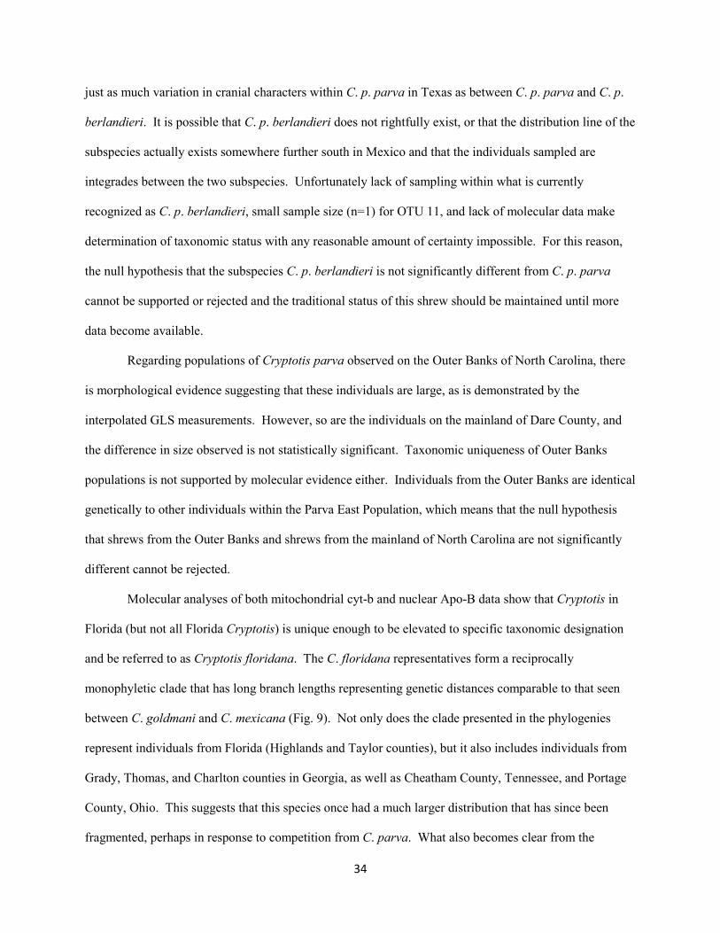
Regarding populations of Cryptotis parva observed on the Outer Banks of North Carolina, there

is morphological evidence suggesting that these individuals are large, as is demonstrated by the

interpolated GLS measurements. However, so are the individuals on the mainland of Dare County, and

the difference in size observed is not statistically significant. Taxonomic uniqueness of Outer Banks

populations is not supported by molecular evidence either. Individuals from the Outer Banks are identical

genetically to other individuals within the Parva East Population, which means that the null hypothesis

that shrews from the Outer Banks and shrews from the mainland of North Carolina are not significantly

different cannot be rejected.

Molecular analyses of both mitochondrial cyt-b and nuclear Apo-B data show that Cryptotis in

Florida (but not all Florida Cryptotis) is unique enough to be elevated to specific taxonomic designation

and be referred to as Cryptotis floridana. The C. floridana representatives form a reciprocally

monophyletic clade that has long branch lengths representing genetic distances comparable to that seen

between C. goldmani and C. mexicana (Fig. 9). Not only does the clade presented in the phylogenies

represent individuals from Florida (Highlands and Taylor counties), but it also includes individuals from

Grady, Thomas, and Charlton counties in Georgia, as well as Cheatham County, Tennessee, and Portage

County, Ohio. This suggests that this species once had a much larger distribution that has since been

fragmented, perhaps in response to competition from C. parva. What also becomes clear from the

35

Fig. 17: Geographic distribution of molecular sequences overlaid onto the interpolated GLS sizes.

Black=C. parva west, Gray=C. parva east, Blue=C. parva (undetermined clade, Parva South), White=C.

floridana.

36

molecular data is that both species (C. floridana and C. parva, and both east and west Parva Populations)

occupy Florida (Fig. 17). Additionally, both species were found in Grady County, Georgia and Taylor

County, Florida.

Revised Distribution

Cryptotis parva appears to contain only two subspecies. The range of C. p. berlandieri was not

altered in this study, pending molecular analyses of the group. C. p. parva, on the other hand, has a range

that spans the majority of the United States from mid-Texas, northern New Mexico (Owen and Hamilton,

1986), mid-eastern Colorado (Siemer et al., 2006), and southern Wyoming (Marquardt et al., 2006) east to

the Atlantic Coast, and from southern Texas, Georgia, and Florida north to South Dakota, Michigan, and

New England (Fig. 18). Apparently, however, the species has been locally extirpated from Michigan and

northern Ohio (Philip Myers, personal communication). The youngest specimen examined for this study

from Michigan or northern Ohio was collected in 1957. Therefore, without more rigorous sampling, the

exact bounds of the northern limits of Cryptotis parva are unknown. Two clades within this species

emerged in the analysis of two mitochondrial markers (cyt-b and COI), one nuclear marker (Apo-B), and

analyses of population genetics (Fig. 17). The Parva West clade consists mostly of samples from states

west of the Mississippi while the Parva East clade consists mostly of samples east of the Appalachian

Mountains. These two clades appear to have a large zone of intergradation between these two landmarks.

The pattern of genetic differentiation marked by the Mississippi River and the Appalachian Mountains

can be seen in other short-tailed shrews of the genus Blarina (Brant and Ortí, 2002; Brant and Ortí, 2003).

'eotoma floridana also was found by Hayes and Harrison (1992) to be a species made up of a western

phylogroup and a northeastern phylogroup.

Cryptotis floridana most likely occupies southern Florida and parts of southern Georgia including

Grady, Thomas, and Charlton counties. It is uncertain if these two populations are connected along the

eastern coast of Florida or have been completely isolated. Isolated populations of C. floridana are also

present in Cheatham Counties, Tennessee and Portage County, Ohio. The specimen from Portage County

37

Fig. 18: Revised distribution of Cryptotis parva and Cryptotis floridana in the United States.

Distributions are derived from the specimen localities resulting from an exhaustive search of museum

databases and recent literature. 1=C. p. berlandieri, 2=C. p. parva, and 3=C. floridana. Mapping

coordinate system is GCS_North_American_1983.

38

was collected in 1940 so, again, it is uncertain if this population persists or has been extirpated. The

revised distributions described are subject to change with more intense sampling in priority areas.

Phenotypic Plasticity and Bergmann’s Rule

One reason that the distinction between species within Florida has gone unobserved for so long

could be explained by the concept of phenotypic plasticity. The morphological data from multiple

statistical tests suggest specimens retain moderate sizes in the majority of the genus’ range in the United

States, but are large in Florida and near the Atlantic Coast, regardless of which species, or clade within

species (in the case of Cryptotis parva) to which they belong. This trend does not appear to be a clinal

increase in size from west to east or north to south, but rather an abrupt increase. Both races of C. parva

are found in Florida, and, both races are larger in Florida than in the remainder of the range. This pattern

occurs with specimens of Cryptotis floridana as well. Those that are found in Florida are large in size,

and those found in isolated pockets of Tennessee (corresponds to OTU 16) and Ohio (OTU 27) are small.

This explains the incongruence between this study and past studies that have been based purely on

phenotypic characters. Cases of phenotypic plasticity demonstrate the importance of using molecular data

in conjunction with morphological data in describing species and assessing evolutionary classifications.

Phenotypic characters can often evolve independently in response to environmental factors, which has

important ecological implications but can confuse phylogenetic relationships (Avise, 2004).

Cryptotis floridana could represent a cryptic species or a sibling species. Molecular techniques

have been very effective in identifying similar cases of cryptic structure in both invertebrates and

vertebrates (Avise, 2000; Peppers and Bradly, 2000; Herbert et al., 2004; Olson et al., 2004; Stuart et al.,

2006), including in other genera as species of shrews (Basset et al., 2006; Dubey et al., 2007). It is

possible, however, that this is not a cryptic species, but that there is a morphological difference between

the two species that has remained unnoticed. Woodman et al. (2003) and Woodman and Morgan (2005)

have proposed morphological differences in the osteology of the humerus and forefeet, respectively, in

species of Cryptotis. Furthermore, the difference between the two species could be due to habitat

39

partitioning or different ecological requirements. Specimens of Cryptotis that are caught in the wild are

usually associated with primary successional habitats such as marshes, meadows, fields, and prairies, but

they have also been collected from mature sand pine scrubs and mesic flatwoods. Kale (1972) reports a

series of almost 200 Cryptotis caught in a mature oak forest in Indian River, Florida (close to the type

locality of C. floridana) during a small mammal census studying the relationships of mosquitoes and their

hosts.

Bergmann’s rule states that animals in colder climates and higher latitudes will generally have

larger body sizes than those of the same species in warmer climates in order to maintain normal body

temperatures. The data collected in this study suggest that Cryptotis parva and Cryptotis floridana are

exceptions to this rule. Correlation analyses indicate that size negatively correlated with latitude, and that

the organisms are largest in Florida and other coastal locations. Ashton et al. (2000) performed a meta-

analysis of body length data available for 110 species of mammals. Although most of the studies

provided support for Bergmann’s rule, some exceptions were observed. The kangaroo rat (Dipodomys)

did not conform to Bergmann’s rule and it was suggested by Best (1981) that seasonality, not

temperature, affected body size. Voles also did not conform to the rule, presumably because of a negative

relationship of temperature and food availability. Finally, two species of weasels were found to conflict

with the rule, possibly because of predator/prey interactions with voles (Ashton et al., 2000). Meiri and

Dayan (2003) performed another review including 149 mammalian species. They found that while

Bergmann’s rule can be used as a generalized pattern in ecology, it is sensitive to mass measurements

rather than linear measurements. In their study they found that animals in the smallest weight class (4-

50g), which included insectivores and rodents, there was no observable validity in the rule. Freckleton et

al. (2003) extended the original dataset of Ashton et al. to include body mass and came to the same

conclusions as Meiri and Dayan (2003) that smaller mammals are less affected by Bergmann’s rule than

larger mammals.

Biogeography

40

Molecular dating of this data indicates that the split between Blarina and Cryptotis happened 13.6

MYA. The isolation and subsequent speciation of Cryptotis parva and Cryptotis floridana (6.1 MYA)

coincides with other lines of evidence suggesting that speciation is often a pre-Pleistocene phenomenon

for many taxa (Zink and Slowinski, 1995; Demboski and Cook, 2001; Avise et al., 2009). An increase in

number of haplotypes around 0.7-0.1 MYA indicates an expansion event suggesting that there was an out-

of-Florida dispersal trend after a period of isolation and subsequent speciation.

All haplotypes within the eastern and western lineages of Cryptotis parva are similar, indicating a

more recent expansion event in these groups. The two radiations of C. parva suggest two source

populations which became isolated about 1.7 MYA towards the beginning of the latest glacial event.

Brant and Ortí (2003) noticed a similar pattern in specimens of Blarina brevicauda and postulated that the

increased water levels of the Mississippi River during interglacial periods would have prevented easy

dispersal of eastern and western isolates across the Mississippi River Valley. Most of the radiation within

the two lineages of Cryptotis parva is concentrated between 1 MYA and 0.2 MYA (mid-late Pleistocene)

and is marked by high haplotype diversity and low nucleotide divergence, which is consistent with

structuring formed by fluctuating glaciations events. The eastern clade began moving west and south out

of a refugia that may have existed somewhere on the East Coast while the western clade began moving

east and south from a refugia possibly existing in the Southwestern United States (Estill and Cruzan,

2001; Sorrie and Weakley 2001). Exact locations of glacial refugia are uncertain, but studies hypothesize

a southwestern refugia having occurred somewhere around northern Texas, Oklahoma, and southern

Kansas (Jones et al., 1984). At the same time that the two lineages of Cryptotis parva were moving

towards the interior of the country, Cryptotis floridana was dispersing from Florida and as the two

lineages of Cryptotis parva began to converge, the competition pressure may have suppressed C.

floridana into isolated pockets.

CONCLUSIONS

Conservation

41

Arguably, the two lineages of Cryptotis parva may fall into the definition of management unit

(MU) given by Moritz (1994) because of the significant divergence between the two clades, however, all

indications produced by population level analyses suggest that both clades within Cryptotis parva are

expanding and maintaining genetic diversity. Furthermore, evidence suggests that this species has a large

geographic distribution that is expanding in the northwest of its range. Therefore, it is more prudent to

focus conservation efforts on its sister species, Cryptotis floridana.

Even though some molecular analyses such as the mismatch distribution suggest that Cryptotis

floridana, as a population, is historically expanding, it is clear that the species is currently undergoing

severe habitat fragmentation and isolation, specifically in northern Ohio and Tennessee. It is possible that

despite the habitat fragmentation, C. floridana so far has managed to maintain genetic diversity within the

populations, possibly due to periods of water level decline during glaciations cycles that may have

allowed more connectivity. Additionally, the species represents an evolutionarily significant unit that is

reciprocally monophyletic to C. parva in mitochondrial and possibly nuclear genes (Moritz, 1994), and

for this reason the species merits conservation. Further study of the isolated pockets of this species may

yield information on what environmental variables allow this species to thrive in these areas. That

information can then be used to model where other pockets may exist, and determine if there is a

possibility of other relict populations in other parts of the United States. The data obtained from such a

modeling study could then be applied to ecosystem based approaches of the conservation of Cryptotis

floridana. If this management technique is applied to Florida, for example, the unique ecology that

allows two species of Cryptotis to coexist would be focused on in its entirety which would positively

benefit other Florida biota. Several species have been found to have unique races that exist only in

Florida (Soltis, 2006; Avise et al., 2009) as evidenced by a typical zone of hybridization or intergredation

along the midsection of the panhandle. Prioritizing conservation of the entire Florida ecology would

serve to conserve two species and three genetic clades of least shrews.

Future Focus

42

The inconclusive placement of the two individuals from St. Johns and Taylor counties in Florida

may be the result of inadequate sampling in this region. Sampling efforts in the future should be

prioritized to areas between these locations and well established haplotypes. It is also necessary to focus

sampling efforts to areas in and around Portage County, Ohio, and Cheatham County, Tennessee, in order

to quantify the frequency and distribution of Cryptotis floridana in these areas.

Furthermore, sampling efforts need to be prioritized in southern Georgia and Florida.

Specifically, there is potentially a second population in Florida as evidenced by the strong support for the

large split between individuals from Charlton and Thomas counties in Georgia from the remainder of the

C. floridana. Furthermore, the branch lengths between these potential C. floridana populations is

comparable to that seen separating the C. parva east and C. parva west clades. More individuals from

this area are needed to confirm this relationship and to further investigate the dynamics within that

population.

Because much of the starting material for molecular analyses was highly degraded and in low

concentrations, only a small fragment of each marker was amplified. It is possible that if the entire

mitochondrial and/or nuclear genomes were sequenced, the phylogenetic signal within the genus would

be improved. With sampling more clearly directed, resources can be used to acquire fresh tissue that will

permit the amplification of larger gene fragments.

Finally, it is important to expand the search of morphological characters that might reflect the

genetic differences observed between C. parva and C. floridana as well as between the two genetic clades

within C. parva. Additionally, it would be useful to test the extent of phenotypic plasticity observed in

cranial characters of the least shrew experimentally.

43

LITERATURE CITED

Arbogast, B. S. 1999. Mitochondrial DNA phylogeography of the New World flying squirrels

(Glaucomys): implications for Pleistocene biogeography, Journal of Mammalogy, 80:142-155.

Ashton, K. G., M. C. Tracy, A. de Queiroz. 2000. Is Bergmann’s rule valid for mammals?. The

American Naturalist, 156(4):390-415.

Avise, J. C. 2000. Phylogeography. Cambridge: Harvard University Press.

Avise, J. C. 2004. Molecular Markers, Natural History, and Evolution. 2nd Ed. Sinauer Associates, Inc.

Publisher, Sunderland, Massachusetts. 684 pp.

Avise, J. C., D. Walker, and G. C. Johns. 2009. Speciation durations and Pleistocene effects on vertebrate

phylogeography. Proceedings of the Royal Society, 2665:1707-1712.

Baird, S. F. 1859. Mammals of North America; The Descriptions of Species Based Chiefly on the

Collections in the Museum of the Smithsonian Institution. Arno Press, New York. 764 pp.

Basset, P., G. Yannic, and J. Hausser. 2006. Genetic and karyotypic structure in the shrews of the Sorex

araneus group: are they independent? Molecular Ecology, 15: 1577-1587.

Best, T. L. 1981. Relationships between ecogeographic and morphologic variation in the agile kangaroo

rat (Dipodomys agilis) in Baja California, Mexico. Bulletin of the Southern California Academy

of Sciences 80:60-90.

Blois, J. L., and B. S. Arbogast. 2006. Conservation genetics of the Sonoma tree vole (Arborimus Pomo)

based on mitochondrial and amplified fragment length polymorphism markers. Journal of

Mammalogy, 87:950-960.

Bole, B. P., Jr., and P. N. Moulthrop. 1942. The Ohio recent mammal collection in the Cleveland

Museum of Natural History. Scientific Publication of the Cleveland Museum of Natural History,

5:83-181.

Brant, S. V., and G. Ortí. 2002. Molecular phylogeny of short-tailed shrews, Blarina (Insectivora:

Soricidae). Molecular Phylogenetics and Evolution, 22:163-173.

Brant, S. V., and G. Ortí. 2003. Phylogeography of the northern short-tailed shrew, Blarina

brevicauda (Insectivora: Soricidae): past fragmentation and postglacial recolonization.

Molecular Ecology, 12:1435-1449.

Choate, J. R. 1970. Systematics and zoogeography of Middle American shrews of the genus Cryptotis.

University of Kansas Publications, Museum of Natural History, 19:195-317.

Churchfield, S. 1990. The natural history of shrews. A & C Black Publisher, London, 178pp.

Clement, M., D. Posada, and K. A. Crandall. 2000. TCS: a computer program to estimate gene

genealogies. Molecular Ecology, 9: 1657-1660.

44

Demboski, J. R., and J. A. Cook. 2001. Phylogeography of the dusky shrew, Sorex monicolus

(Insectivora, Soricidae): insight into deep and shallow history in northwestern North

America. Molecular Ecology, 10:1227-1240.

Drummond A. J., and A. Rambaut. 2007. BEAST: Bayesian evolutionary analysis by sampling trees.

BMC Evolutionary Biology, 7:214.

Dubey, S., N. Salamin, S. D. Ohdachi, P. Barrière, and P. Vogel. 2007. Molecular phylogenetics of

shrews (Mammalia: Soricidae) reveal timing of transcontinental colonizations. Molecular

Phylogenetics and Evolution, 44:126-137.

Estill, J. C., and M. B. Cruzan. 2001. Phytogeography of rare plant species endemic to the

southeastern United States. Castanea, 66:2-23.

Excoffier, L. G. Laval, and S. Schneider. 2005. Arlequin ver. 3.0: An integrated software

package for population genetics data analysis. Evolutionary Bioinformatics Online :47-50.

Felsenstein, J. 2004. Inferring phylogenies. Sinauer Associates, Inc., Massachusetts, 664pp.

Freckleton, R. P., P. H. Harvey, and M. Pagel. 2003. Bergmann’s rule and body size in mammals. The

American Naturalist, 161(5):821-825.

Fumagalli, L., P. Taberlet, D. T. Stewart, L. Gielly, J. Hausser, and P. Vogel. 1999. Molecular

phylogeny and evolution of Sorex shrews (Soricidae: Insectivora) inferred from mitochondrial

DNA sequence data. Molecular Phylogenetics and Evolution, 11(2):222-235.

Genoways, H. H., and J. R. Choate. 1972. A multivariate analysis of systematic relationships among

populations of the short-tailed shrew (genus Blarina) in Nebraska. Systematic Zoology, 21:

106-116.

Guindon, S., and O. Gascuel. 2003. A simple, fast, and accurate method to estimate large phylogenies by

maximum-likelihood. Systematic Biology, 52:696-704.

Hafner, D. J., and C. J. Shuster. 1996. Historical biogeography of western peripheral isolates of the

least shrew, Cryptotis parva. Journal of Mammalogy, 77:536-545.

Hall, E. R., 1981. The Mammals of North America. Second ed. John Wiley and Sons, New York, 1271pp.

Hall, E. R., and K. R. Kelson. 1959. The mammals of North America. Ronald Press, New York,

1241pp.

Handley, C. O., Jr., and M. Varn. 1994. Identification of the Carolinian shrews of Bachman 1837.

pp.393-406. In Advances in the Biology of Shrews (J. F. Merritt, G. L. Kirkland Jr., and R. K.

Rose, eds.), Special Publication, Carnegie Museum of Natural History, 18.

Harris, A. H. 1998. Fossil history of shrews in North America, pp. 133-156. In Evolution of Shrews.

Mammal Research Institute, Polish Academy of Sciences, (Wójcik, J. M., and M. Wolsan, eds.)

Bialowieza.

Harrison, R. G. 1989. Animal mitochondrial DNA as a genetic marker in population and evolutionary

biology. Trends in Ecology and Evolution, 4:6-11.

45

Hayes, J. P., and R. G. Harrison. 1992. Variation in mitochondrial DNA and the biogeography history of

woodrats ('eotoma) of the Eastern United States. Systematic Biology, 42:331-344.

Herbert, P. D. N., E. H. Penton, J. M. Burns, D. H. Janzen, and W. Hallwachs. 2004. Ten species in one:

DNA barcoding reveals cryptic species in the neotropical skipper butterfly Astraptes fulgerator.

PNAS, 101:14812-14817.

Hoffmeister, D. F. 2002. Mammals of Illinois. University of Chicago Press, Chicago, IL 384pp.

Hutchinson, S. 2007. Morphological variation in the insectivores of North Carolina. Unpublished

Honors Thesis, University of North Carolina Wilmington., Wilmington, North Carolina, 54pp.

Irwin, D. M., T. D. Kocher, and A. C. Wilson. 1991. Evolution of the cytochrome b gene of

mammals. Journal of Molecular Evolution, 32:128-144.

Jackson, H. H. T. 1961. Mammals of Wisconsin. University of Wisconsin Press, Madison,

Wisconsin, 504 pp.

Kale II., H. W. 1972. A high concentration of Cryptotis parva in a forest in Florida. Journal of

Mammalogy, 53:216-218.

Kocher, T. D., W. K Thomas, A. Meyer, S. V. Edwards, S. Pääbo, F. X. Villablanca, and A. C. Wilson.

1989. Dynamics of mitochondrial DNA evolution in animals: amplification and sequencing with

conserved primers. Proceedings from the National Academy of Sciences, 86:6196-6200.

Lowery, G. H., Jr. 1974. The mammals of Louisiana and its adjacent waters. Louisiana State University

Press. 565pp.

Lyon, J. W., Jr. 1936. Mammals of Indiana. American Midland Naturalist, 17:1-373.

Marquardt. 2006. First record of the least shrew in Wyoming. Prairie Naturalist, 38:195-196.

Meiri, S., and T. Dayan. 2003. On the validity of Bergmann’s rule. Journal of Biogeograhy, 30:331-351.

Merriam, C. H. 1895. Revision of the shrews of the American genera Blarina and Notiosorex. North

American Fauna, 10:5-34.

Moncrief, N. D., J. R. Choate, and H. H. Genoways. 1982. Morphometric and geographic relationships

of short-tailed shrews (Genus Blarina) in Kansas, Iowa, and Missouri. Annals of Carnegie

Museum, 51:157-180.

Moritz, C. 1994. Defining ‘evolutionary significant units’ for conservation. Trends in Ecology and

Evolution, 9:373-375.

Mumford, R. E., and J. O. Whitaker, Jr. 1982. Mammals of Indiana. Indiana University Press,

Bloomington, 537 pp.

Olson, K. E., S. M. Goodman, and A. D. Yoder. 2004. Illumination of cryptic species boundaries in

long-tailed shrew tenrecs (Mammalia: Tenrecidae; Microgale), with new insights into

46

geographic variation and distributional constraints. Biological Journal of the Linnean Society,

83:1-22.

O’Neill, M. B., D. W. Nagorsen, and R. J. Baker. 2005. Mitochondrial DNA variation in water shrews

(Sorex palustris, Sorex bendirii) from western North America: implications for taxonomy and

phylogeography. Canadian Journal of Zoology, 83:1469-1475.

Owen, R. D., and M. J. Hamilton. 1986. Second record of Cryptotis parva (Soricidae: Insectivora) in

New Mexico with a review of its status on the Llano Estacado. Southwestern Naturalist,

31:403-405.

Peppers, L. L., and R. D. Bradley. 2000. Cryptic species in Sigmodon hispidus: Evidence from DNA

sequences. Journal of Mammalogy, 81:332-343.

Posada, D. 2008. JModelTest: phylogenetic model averaging. Molecular Biology and Evolution, 25:

1253-1256.

Raun, G. G. 1965. Cryptotis parva from Coahuila, Mexico and comments on the taxonomy of least

shrews in Texas. The Southwestern Naturalist, 10(3):214-218.

Shinohara, A., K. L. Cambell, and H. Suzuki. 2003. Molecular phylogenetic relationships of moles,

shrew moles, and desmans from the new and old worlds. Molecular Phylogenetics and

Evolution, 27:247-258.

Siemer, J. L., Y. R. Chen, K. M. Canstorp, J. R. Sovell, and K. L. Cornelisse. 2006. Range Expansion of

the least shrew (Cryptotis parva) in Colorado. The Southwestern Naturalist, 51:267-269.

Sorrie, B. A., a. S. Weakley. 2001. Coastal Plain vascular plant endemics: phytogeographic

patterns. Castanea, 66:50-82.

Stuart, B. L., R. F. Inger, and H. K. Voris. 2006. High level of cryptic species diversity revealed by

sympatric lineages of Southeast Asian forest frogs. Biology Letters, 2:470-474.

Swofford, D. 2003. PAUP*: phylogenetic analysis using parsimony (*and other methods). Sinauer

Associates, Inc., Publishers, Sunderland, Massachusetts.

Webster, W. D., J. F Parnell, and W. C. Biggs, Jr. 1985. The mammals of the Carolinas, Virginia, and

Maryland. University of North Carolina Press, Chapel Hill, North Carolina, 255 pp.

Whitaker, J. O, Jr. 1974. Cryptotis parva. Mammalian Species, 43:1-8.

Whitaker, J. O., Jr., and W. J. Hamilton, Jr. 1998. The Mammals of the Eastern United States. Cornell

University Press, Ithaca, New York, 581 pp.

Woodman, N. and R. M. Timm. 2000. Taxonomy and evolutionary relationships of Phillips’ small-eared

shrew, Cryptotis phillipsii (Schaldach, 1966), from Oaxaca, Mexico (Mammalia: Insectivora:

Soricidae). Proceedings of the Biological Society of Washington, 113: 339-335.

Woodman, N., C. A. Cuartas-Calle, and C. A. Delgado-V. 2003. The humerus of Cryptotis

colombiana and its bearing on the species phylogenetic relationships (Soricomorpha:

Soricidae). Journal of Mammalogy, 84:832-839.

47

Woodman, N., and J. P. Morgan. 2005. Skeletal morphology of the forefoot in shrews (Mammalia:

Soricidae) of the genus Cryptotis, as revealed by digital x-rays. Journal of Morphology, 266:60-

73.

Zink R. M., and J. B. Slowinski. 1995. Evidence from molecular systematic for decreased avian

diversification in the Pleistocene Epoch. Proceedings of the National Academy of

Sciences, 92:5832-5835.

48

Appendix I

Canada

Ontario (n=2). 'orfolk County: Longpoint (1 ROM, 1 USNM).

United States

Arkansas (n=11). Benton County: 9 mi N Bentonville (1 KU). Desha County: White River

National Wildlife Refuge (1 NMNH). Logan County: 11 mi W New Blaine, jct SR 197 & SR 22 (2 CU).

Ouachita County: Camden (1 NMNH). Washington County: 3 mi SE Winslow (1 KU); 1.5 mi S

Winslow (5 KU).

Alabama (n=22). Clarke County: Jackson (1 NMNH). Clay County: Talladega National Forest

(1 CU). Dekalb County: Mentone, Lookout Mountain (2 AMNH). Jackson County: Hogwood Ridge,

1.4 mi S Tennessee border (1 NCSM); 0.5 mi N Money Hollow, 0.75 mi E Rt 79, Jack Gap (4 NCSM);

Woodville (1 NMNH). Lee County: Auburn (1 KU). Marshall County: Cane Creek, 6 mi N Oleander (1

NMNH ). Mobile County: Alabama Port (1 NMNH). Montgomery County: Barachias (7 NMNH).

Talapaloosa County: HOBE, Horseshoe Bend (1 NMNH). County Unknown: Sand Mountain (1

NMNH).

Colorado (n=20). Larimer County: 1.8 mi N, 0.5 mi E Fort Collins, Willox Lane (15 MSB). Kit

Carson County: 4 mi E Flagler (1 KU). Morgan County: 2 mi N, 2.5 mi W Fort Morgan (2 KU). Yuma

County: 1 mi E Laird (2 KU).

Connecticut (n=1). Middlesex County: Westbrook Salt Marsh (1 AMNH).

Delaware (n=3). 'ew Castle County: Delaware City (2 NMNH); 1.5 mi N Odessa (1 NMNH).

Florida (n=185). Alachua County: South Gainesville, Paynes Prairie, Hailes Landing (3

UMMZ); 6 mi E Gainesville (4 UMMZ); 5 mi NW Hawthorn (3UMMZ); La Crosse (3 NMNH). Baker

County: Glen St Mary (4 NMNH); Osceola National Forest, Junction 1-10, FSR 263 (1 FLMNH).

Bradford County: exact location unknown (2 FLMNH). Brevard County: Canaveral (1 NMNH);

Floridana Beach (1 NCSM); Georgiana (1 NMNH); Grant (1 ROM); Oak Lodge (2 MCZ); Oak Lodge, E

49

Penn Opp Micco (12 MCZ). Charlotte County: Englewood (3 FMNH). Colombia County: Lake City (1

NMNH); Osceola National Forest (1 FLMNH). Dade County: Hialeah (1 KU); WSW Kendall (1 KU); 4

mi W Kendall (1 KU); Miami, 108 St (3 KU). Dixie County: Oldtown (1 NMNH). Duval County:

TIMU, Thomas Creek (1 UNCW). Escambia County: Pensacola (1 NMNH). Franklin County: 8 mi

SSE Panacea, Alligator Point (2 NMNH). Hardee County: 4 mi N, 4 mi E Duetee (1 KU); 0.5 mi SE

Fort Green Springs (1 KU); 1 mi S Fort Green Springs (1 KU); 2 mi N, 1 mi E Fort Green Springs (1

KU). Highlands County: Archbold Biological Station (1 FMNH, 1 FLMNH); Archbold Biological

Station, 8 mi S Lack Placid (8 FLMNH); 8 mi E Archbold Biological Station, Buck Island Ranch (3

FMNH); Avon Park (3 NCSM); Gould Unit (1 FLMNH); Hicoria, Archbold Biological Station (1

FMNH); Highlands Hammock State Park (1 FMNH); 4 mi N Lake Placid, near Lake Francis (9

FLMNH); Royce Unit (2 FLMNH); SR 70, 7.5 mi Hwy 27 (1 FMNH); Exact location unknown (1

FMNH). Hillsborough County: 2 mi N, 2 mi E Fort Lonesome (1 KU); 1 mi N Picnic (1 KU); 1 mi N, 4

mi W Picnic (1 KU). Lake County: Clermont, 0.5 mi NW Citrus Tower on US 27 (1 FLMNH). Leon

County: AKE Iamonia, Tall Timbers Inc. (1 GMNH); 3 km W Tallahassee (1 LSU). Levy County: 18 mi

SW Otter Creek (1 FLMNH); salt marsh on Wacosassa Bay (1 FLMNH). Madison County: Ellaville,

vicinity of Ellaville (1 FLMNH); Madison (5 NMNH). Marion County: McIntosh (1 NMNH); Ocala

National Forest (1 GMNH). Monroe County: Key Largo (2 KU). Pinellas County: exact location

unknown (3 FLMNH). Polk County: Arbuckle State Forest (1 FMNH); 6 mi SW Bartow (2 KU); 6 mi S,

1 mi W Bartow (1 KU); 0.5 mi S, 2 mi W Brewster (1 KU); 1.5 mi S, 3 mi E Brewster (1 KU); 2 mi S

Brewster (1 KU); Flaming Arrow Boy Scout Camp (1 FMNH); 1 mi S, 7 mi W Fort Meade (1 KU); 15

mi SW Fort Meade (1 KU); Lakeland (1 NCSM); Lakeland, Orange Park Study Area (1 NCSM); Orange

Park (1 NCSM). Putnam County: 3 mi E Melrose, Smith Lake Sandhill, Ordway Preserve (3 FLMNH);

Ordway Preserve (9 FLMNH); Rodman (6 FLMNH); Welaka (2 FLMNH); Welaka Preserve (1

FLMNH); 1 mi S Welaka, University of Florida Conservation Reserve (5 UMMZ). Santa Rosa County:

Girl Scout on S Shore of Pensacola (1 FMNH). St Johns County: south end of Anastasia Island, 15 mi S

St Augustine (1 AMNH); Carterville (3 MCZ); Summer Haven (2 MCZ); Tolomata River, St Johns Rd

50

158 (1 FLMNH). Taylor County: 4 mi NNW Perry (2 AMNH, 1 KU); 4 mi NNW Perry, Blanham Farm

(1 AMNH); 4 mi SW Perry (1 AMNH, 1 KU); 5 mi N Salem, Hwy 19/98 (1 UNCW). Volusia:

Enterprise (1 FMNH). Wakulla County: St Marks National Wildlife Refuge (1 FMNH, 2 NMNH); St

Marks National Wildlife Refuge, Panacea Unit (4 NMNH); St Marks National Wildlife Refuge, St Marks

Unit (9 NMNH). Walton County: 3 mi W Freeport on Hwy 20 (1 FLMNH). Washington County:

Chipley (1 KU). County Unknown: exact location unknown (1 FMNH).

Georgia (n=123). Appling County: 3 mi E Baxley (1 GMNH). Berrian County: 11 km E

Nashville (1 NMNH). Bulloch County: Statesboro city limits (1 KU); 3 mi N Statesboro (2 KU); 5 mi N

Statesboro (2 KU). Ben Hill County: Fitzgerald (2 GMNH). Bryan County: Fort Stewart, Hwy 144, 4

km W Hwy 67 jct (1 GMNH). Burke County: Di-Lane Plantation Wildlife Management Area (3 GMNH).

Camden County: St Mary’s (2 MCZ). Charlton County: Cowhouse Island, TT-14 Rd, Union Camp

Land, Crew’s Circle (1 GMNH); Okefenokee Swamp, Billy’s Island (2 CU); Okefinokee Swamp, Race

Pond, King’s Canal (1 CU); 2 mi S Race Pond (1 AMNH). Chatham County: Skiddaway Island (1

MCZ). Clarke County: Athens (11 GMNH, 1 KU); Athens, College Station Road, Horseshoe Bend (1

GMNH); Athens, across river from UGA poultry (1 GMNH); Athens, Alps Rd field (1 GMNH); Athens,

River Rd dump (1 GMNH); Athens, near Lake Kirota (2 GMNH); 1 mi SE Athens (3 GMNH); I-13 (1

GMNH); Sandy Creek (1 GMNH). Cobb County: Kennesaw Mountain (2 UNCW). Dekalb County:

Atlanta, Panthersville Road, Georgia State University Property (1 GMNH); Clarkston, field at intersection

of Stone Mt Freeway and Montreal Rd (2 GMNH). Emanuel County: Blundale, 14 km S Wadley, off FA

Hwys 1 & 4 (1 GMNH). Grady County: Beachton (3 FLMNH, 5 NMNH); Beachton, Birdsong

Plantation (4 NMNH); 4 mi S Beachton, Birdsong Plantation (5 NMNH); Beachton, Sherwood Plantation

(11 NMNH). Greene County: Greensboro (1 GMNH). Gwinnett County: CHAT, Abbott’s Bridge (2

UNCW). Liberty County: 0.7 mi S, 0.3 mi W of Canoochee River & Hwy 119 intersection (2 GMNH);

Ft Stewart (4 KU); Riceboro, LeConte Plantation (4 NMNH); exact location unknown (1 NMNH).

McIntosh County: Sapelo Island, various sites (7 GMNH). Muscogee County: Ft Benning, array 5 (3

GMNH). Montgomery County: Chatham (1 UMMZ); exact location unknown (8 MCZ). Olgethorpe

51

County: 10 mi SW Crawford (6 GMNH); Colbert, Angus Farm (1 GMNH). Tift County: 2 km E Tifton

(2 GMNH). Thomas County: Boston (1 NMNH); Metcalf (1 FLMNH); Thomasville, Spring Hill (1

UMMZ).

Iowa (n=25). Boone County: Polly Creek (2 NMNH). Decatur County: Leon (2 NMNH).

Fremont County: 3 mi S, 9 mi W Sidney (1 KU). Lee County: Montrase (1 NMNH); Washington (2

NMNH); Jefferson (3 NMNH). Montgomery County: Red Oak (5 NMNH). Story County: Ames (1

NMNH). Cass County: Atlantic (1 NMNH). Des Moine County: 2 mi W, 1 mi N West Burlington (1

KU). Keokuk County: Sigourney (1 KU). Mahaska County: 3.5 W Oskaloosa (3 KU). Monona County:

0.5 mi S, 2 mi W Moorhead (1 KU). Van Buren County: Lasey, Keosagua State Park (1 NMNH).

Illinois (n=37). Alexander County: Cache (1 FLMNH). Champaign County: SW Champaign (1

INHS); Fisher (1 INHS); Mayview (1 INHS); Phillips Tract (1 INHS); Seymour (2 INHS); Trelease

Prairie (2 INHS); Trelease Woods (1 INHS); Urbana (6 INHS); 1.5 mi SW University of Illinois (1

INHS); 1.25 mi N Urbana (1 INHS); 2 mi S Urbana (1 INHS); 2.5 mi S Urbana (2 INHS); 3 mi E, 1 mi N

Urbana (6 INHS); 4 mi E Urbana (1 INHS); 4 mi E Urbana, Mayview Prarie (1 INHS); 5 mi NE Urbana

(3 INHS). Dekalb County: Cortland (1 NMNH). Jasper County: 7 mi SW Newton (1 MSB). McClean

County: Bloomington, Archibuteo (1 NMNH). Piatt County: 5 mi W, 2.5 mi S Monticello Allerton Park

(1 FLMNH). Wabash County: exact location unknown (1 NMNH).

Indiana (n=88). Allen County: 0.25 mi N New Haven (1 NMNH). Benton County: 8 mi N

Harold, Otterbein (1 NMNH). Clay County: 1 mi W Brazil (2 NMNH). Crawford County: Wyandotte

(1 NMNH). Daviess County: 4 mi E Odon (1 NMNH). Dearborn: Bright (1 NMNH). Floyd County: 6

mi N New Albany on Rt 111 (1 NMNH); 1 mi S St Joseph (1 NMNH). Fountain County: Attica (1

NMNH); 2 mi SE Wallace (1 INHS). Franklin County: Blooming Grove (1 NMNH). Fulton County:

0.5 mi W Rochester (1 NMNH). Gibson County: 1 mi S Patoka (1 NMNH). Jackson County: Kurtz (1

FMNH). Jenmings County: Crasley Fish and Game Area (1 NMNH). Johnson County: 0.25 mi W

Edinburg (1 NMNH). Knox County: Bicknell (1 NMNH). Marion County: exact location unknown (1

NMNH). Martin County: Crane (1 NMNH); Crane, Naval Ammunition Depot (1 ROM). Monroe

52

County: 2 mi SE Bloomington (1 UMMZ). Montgomery: 3 mi S Waynetown (1 NMNH). Orange

County: exact location unknown (1 NMNH). Owen County: 3 mi E Spencer, entrance to McCormic

Creek State park (2 INHS). Perry County: Cannelton (1 NMNH). Pike County: 2 mi SE Coe, Purdue-

Enos Study Area (1 NMNH); 2 mi N Spurgeon, Purdue-Enos Study Area (9 NMNH). Porter County:

Exact location unknown (1 NMNH). Posey County: Hovey Lake (7 UMMZ); W Hovey Lake (1

UMMZ); exact location unknown (1 UMMZ). Putnam County: 0.5 mi W Pleasant Gardens (1 NMNH).

Ripley County: Rexville (5 NMNH); 0.5 mi E Rexville (4 NMNH); 0.5 mi E, 0.25 mi S Rexville (1

NMNH). Sullivan County: exact location unknown (1 UMMZ). Tippecanoe County: west Lafayette (5

NMNH); 10 mi W Lafayette (7 NMNH); exact location unknown (3 NMNH). Vigo County: Terra Haute

(1 NMNH); 1 mi S Terre Haute (3 INHS); 6 mi W Terre Haute (1 INHS). Warrick County: 5 mi N

Newburgh (5 NMNH). Washington County: 3 mi N Smedley (4 NMNH).

Kansas (n=103). Anderson County: 1 mi N, 1.5 mi E Colony (1 KU); 3.7 mi S Garnett (1 KU); 2

mi S, 0.5 mi W Welda (1 KU). Atchison County: 1.5 mi S Muscotah (1 KU). Barber County: Plum

Thicket, Sharon (1 KU); 3 mi N, 1 mi E Sharon (1 KU); 5 mi N, 0.5 mi E Sharon (1 KU); 5 mi N, 1.5 mi

E Sharon (5 KU). Butler County: 1 mi N Towanda (1 KU). Cherokee County: 1 mi S Baxter Springs (1

KU); 2 mi N Baxter Springs (1 KU); 2 mi N, 0.5 mi W Baxter Springs (2 KU); 0.33 mi N, 6 mi E Baxter

Springs (1 KU); 2 mi S, 1 mi E Galena (1 KU). Coffey County: 2.5 mi S Burlington (1 KU). Cowley

County: 8.1 mi E Arkansas City (1 KU); 2 mi S, 0.5 mi W Udall (1 KU). Doniphan County: Geary (2

KU); 0.2 mi N Troy (1 KU). Douglas County: Lawrence (1 AMNH, 6 CU, 2 INHS, 1 UMMZ, 2

NMNH); 1 mi W Lawrence (3 MSB); 2 mi SW Lawrence (1 ROM); 1 mi E, 2 mi S Lawrence (1

FLMNH); 1 mi S, 8 mi W Lawrence (5 NMNH); 5 mi N Lawrence (4 NMNH); University of Kansas,

Lawrence, Prairie Acre (1 FLMNH); exact location unknown (1 UMMZ). Ellis County: 11.25 mi N, 0.5

mi E Victoria (1 KK). Greenwood County: 0.25 mi E Hamilton (4 UMMZ). Hodgeman County: 0.5 mi

S, 5 mi E Kalvesta (1 KK). Jefferson County: 14 km NE Lawrence (1 NMNH). Kingman County: quail

farm (2 KU). Leavenworth County: Tom Searingen’s House (4 KU). Linn County: 6 mi N Pleasanton

(2 INHS). Lyon County: Emporia Bluestem Prairie Meadow (1 UMMZ). Meade County: 1.5 mi N

53

Fowler (9 KU); Meade State Park (1 INHS); Meade County State Lake, Old CCC barracks (6 KU); 1 mi

SW Meade (1 KU); 8 mi S, 6 mi W Meade (1 KU); 17 mi S Meade (6 KU); 17 mi SW Meade (1 KU, 1

UMMZ). Riley County: exact location unknown (4 UMMZ). Wabaunsee County: 3 mi S, 3.7 mi E

Alma (1 KK). County Unknown: eastern Kansas (2 KU); 1.5 mi SW Hayes (1 NMNH).

Kentucky (n=23). Crittenden County: Floodplain of Tradewater river, 13 air km W SR 120 and

river (1 NMNH). Edmonson County: 1 mi S Brownsville (1 NMNH); 11 mi S Brownsville (1 NMNH).

Franklin County: 2.2 km S Peaks Mill Rd & Holt Dr (1 NMNH). Hopkins County: 9 mi NE

Madisonville (2 NMNH). Kent County: Trigg, 8 mi NNE Golden Pond (1 UMMZ). Logan County: 1.3

km W jct. SR 106 & US 431 (3 NMNH). Meade County: 2 mi SE Bradenburg Station (2 NMNH). Ohio

County: 2 mi NE Hartford (1 NMNH). Rockcastle County: 6 mi S Berea (2 NMNH). Trigg County:

Canton (8 NMNH).

Louisiana (n=42). Acadia Parish: Mermentau (12 FMNH). Caldwell Parish: Columbia (5

FMNH). East Baton Rouge Parish: Exact location unknown (1 UMMZ). Saint Landry Parish: 10 km S

Opelousas (1 LSU). Saint Martin Parish: Butte La Rose (2 LSU); 8 km N Catahoula on outer W levee

(1 LSU); Henderson (3 LSU); 1 km N Henderson (1 LSU); 2 km S Henderson, along levee (2 LSU); 6 km

N Henderson on the levee (2 LSU); 14 km S Henderson (1 LSU); 2 km W Saint Martinville (8 LSU).

Washington Parish: Hackley (3 FMNH).

Maryland (n=68). Accomack County: Chincoteague Island (1 NMNH). Allegheny County: 9 mi

S Old Town (1 NMNH). Anne Arundel County: Annapolis, 4 mi W Broom Sage (1 NMNH); 2 mi N

Annapolis (1 NMNH). Baltimore County: Baltimore (1 NCSM); Loch Raven Reservoir, east of Dulaney

Valley Road (1 NMNH). Calvert County: Solomons (1 NMNH); 0.75 mi N Solomon Island (7 NMNH).

Charles County: Port Tobacco (1 NMNH). Dorchester County: Cambridge (5 KU, 4 MCZ, 2 ROM, 3

UMMZ); Cambridge, Blackwater Refuge (1 NMNH). Hartford County: exact location unknown (1

NMNH). Montgomery County: Bethesda (1 NMNH). Prince George’s County: Laurel (3 NMNH);

Patuxent Research Refuge (6 NMNH); Oxon Hill (2 NMNH). Queen Anne’s County: Parsons Island (1

NMNH). Somerset County: Irish Grove (1 NCSM). Worcester County: Assateague National Seashore

54

(6 KU); between Snow Hill & Assateague (1 NCSM); Chincoteague Bay (1 NMNH); Mills Island (4

NMNH); 4 mi S Ocean City, Assateague Island (2 NMNH); 5 mi S Ocean City, Assateague Island (5

NMNH); 15 mi S Ocean City, Assateague Island (1 NMNH); Pocomoke Cypress Swamp (1 NMNH); 5

mi SE Snow Hill, Chincoteague Bay (2 NMNH).

Michigan (n=37). Lenawee County: Adrian (1 NMNH). Washtenaw County: Ann Arbor (7

UMMZ); 5.5 mi SW Ann Arbor (1 UMMZ); 6 mi ENE Ann Arbor (6 UMMZ); Pittsfield (2 UMMZ);

Portage Lake (2 UMMZ); 1 mi W Superior Twp (1 UMMZ); Whitmore Lake (16 UMMZ); Ypsilanti,

Michigan State Normal (1 UMMZ).

Mississippi (n=15). Adams County: Washington (2 NMNH). Kalamazoo County: Vicksburg (4

NMNH). Marshall County: Wall Doxey State Park (9 KU).

Missouri (n=33). Adair County: 5 mi S Kirksville (2 NMNH); 5 mi N, 2 mi W Kirksville (11

FMNH); 6 mi N Kirksville (1 INHS). Clay County: Greenfield Village, NHC (1 KU). Jackson County:

4 mi NE Independence (1 KU); exact location unknown (1 UNCW). Lewis County: 8 mi N Lewiston,

Deer Ridge Wildlife Area (3 KU). Macon County: 5 mi N, 1 mi W Macon, Atlanta Wildlife Area (1

KU); 8.5 mi N Macon, Atlanta Wildlife Area (1 KU). 'odaway County: 5 mi ENE Maryville (2

NMNH). Pettis County: Sedalia (1 NMNH); 4 mi NW Sedalia (1 KU). Saline County: Marshal (1

UMMZ). Saint Charles County: Portage des Sioux (3 NMNH). County Unknown: Exact location

unknown (3 UNCW).

Nebraska (n=38). Cass County: 0.3 mi S, 2 mi W Weeping Water (1 KU); 0.4 mi N, 2 mi W

Weeping Water (7 KU); 1 mi N, 2 mi W Weeping Water (2 KU); 2 mi N, 2 mi W Weeping Water (1

KU); 3 mi N, 2 mi W Weeping Water (1 KU). Douglas County: Omaha, 8240 Keystone Dr (2 KU).

Dundy County: 2 mi SW Bendelman (1 KU); 5 mi N, 2 mi W Parks (1 KU). Gage County: 2 mi W, 1

mi S Barnston (1 KU). Keith County: 4 mi NNW Keystone (1 KU). Lancaster County: College View (1

FMNH); Lincoln (1 AMNH); West Lincoln (1 AMNH); West Lincoln, nr. Oak Creek (1 AMNH).

Pawnee County: 8 mi W, 4 mi S Pawnee City (1 KU). Red Willow County: 8 mi S, 3 mi E McCook (1

KU). Sarpy County: Fort Crook (2 AMNH). Washington County: Blair (12 NMNH).

55

New Jersey (n=6). Atlantic County: 0.7 mi ESE Oceanville, Brigantine National Wildlife Refuge

(4 NMNH). Burlington County: Burlington, near junction Wading River and Head’s Creek (1 CU).

Ocean County: ca. 6 mi SSE Tuckerton (1 NCSM).

New Mexico (n=3). Quay County: W side of Tucumcare Lake (1 MSB); 1.1 km SW Tucumcari

Lake (1 MSB); 6.5 mi SW Tucumcari Airport (1 MSB).

New York: (N=5). Orange County: West Point (2 NMNH). Richmond County: Staten Island,

Richmond (1 AMNH); Staten Island, New Dorp (1 AMNH). Wayne County: North Rose (1 NMNH).

North Carolina (n=479). Alexander County: 6 km NW Ellendale (1 UNCW). Beaufort County:

Aurora (1 UNCW); Aurora Texas Gulf (4 UNCW); 4 km N Aurora (1 UNCW); 6 km N Aurora (14 UNCW); 3

km N South Creek. Bertie County: exact location unknown (2 UMMZ). Bladen County: Hwy 210 at Holly

Creek (1 UNCW); 6 km ENE White Lake (1 NCSM). Brunswick County: 3 km SE Ash (2 UNCW); Belville (6

UNCW); Belville, 5.3 km W Wilmington (1 UNCW); Ev-henwood (3 UNCW); 5 km NE Freeland, SR 1335 (4

UNCW); Lincoln Plant (8 UNCW); near Rabontown (1 UNCW); 1 km N Rabontown (1 UNCW); 1 km NW

Rabontown (1 UNCW); 2 km NW Rabontown (4 UNCW); 19 km WSW Shallotte (1 UNCW); 9 km W

Wilmington (1 UNCW). Buncombe County: Enka (2 UMMZ); Leister (1 UNCW); Little Pisgah (1 NCSM);

Weaverville (2 AMNH). Burke County: 5 km W Ramsey (3 UNCW). Carteret County: 10 km NE Beaufort

(2 NMNH); Croatan National Forest (2 NCSM); 5 km ENE Harlowe (1 NCSM); 9 km S Merriman (5 NCSM);

Morehead City, Bogue Island (2 NMNH). Chowan County: 2 km W Edenton, Hwy 17 (1 UNCW); 7 km SE

Edenton (1 NCSM); 7 air km SE Edenton (2 NCSM); 14 km E Edenton, Sommerset Farm (1 NCSM); 9 km

NE Maysville (1 NCSM); 9 km NW Valhalla (2 NCSM); exact location unknown (2 UNCW). Columbus

County: 5 km NE Freeland, SR 1335 (2 UNCW). Craven County: Corner of Schull Road and Braxton Road

(3 UNCW); End of Browns Farm Rd (8 UNCW); 2 km NNW Rhems (1 UNCW). Cumberland County:

Gallberry Rd (1 UNCW); 2 km SSE Hope Mills (8 UNCW); 3 km S Vander, SR 2010 (8 UNCW). Currituck

County: 1 km S Currituck (2 UMMZ); 5 km W Moyock (1 NCSM). Dare County: Bodie Island (13 UNCW);

Bodie Island, S Nags Head (1 UNCW); Bodie Island, Oregon Inlet (1 UNCW); Buxton (1 NCSM, 2 UMMZ, 1

56

UNCW); 3 km WSW Buxton (1 NCSM); Cape Hatteras (1 AMNH, 1 UNCW); Little Kinnakeet (4 UNCW);

Nagshead, Cape Hatteras (1 UNCW); Stumpy Point (1 NMNH); 13 km SW Stumpy Point (4 NMNH); 16 km

SW Stumpy Point (1 NMNH); exact location unknown (1 NCSM, 1 UMMZ). Duplin County: 4 km ENE

Magnolia, I-40 (8 UNCW); 4 km ESE Magnolia, I-40 (1 UNCW); 4 km W Magnolia, I-40 (2 UNCW); 2.5 km E

Rose Hill, I-40 (3 UNCW); 5 km ESE Rose Hill, SR 1148 (1 UNCW); Wallace (2 UNCW); 4 km SSW Warsaw,

I-40 (1 UNCW); 4 km W Warsaw, Hwy 24 (16 UNCW); 5 km S Warsaw, I-40 (5 UNCW); 5.5 km S Warsaw,

I-40 (1 UNCW); 5 km S Watha, I-40 (1 UNCW). Durham County: Durham (1 NCSM); exact location

unknown (1 NMNH). Edgecombe County: 6 km ESE Battleboro, Davenport Farm (2 NCSM); ca. Swift

Creek, Davenport Farm (3 NCSM). Forsyth County: Bethbara (1 MVZ, 1 NCSM). Gates County: 6 km

WSW Corapeake (1 NCSM); 4 km E Gatesville (1 NCSM). Greene County: 7 km S Snowhill, Hwy 258 (1

UNCW). Guilford County: Greensboro (3 UNCW). Hertford County: 2 km NW Akshoski (4 UNCW); mi S

Winton off Rt 13 (1 NMNH); 5 km SE Winton, Hwy 45 (1 UNCW); exact location unknown (2 UNCW).

Hoke County: 6 km W Raefod, Hwy 211 (1 UNCW); 12 km NE Raeford, Fort Bragg (1 NCSM); exact

location unknown (1 NCSM). Hyde County: 9 km NW Engelhard (9 UNCW); 16 km N Engelhard (2

NMNH); 5 km W Lake Landing (7 NMNH); Lake Mattamusket National Wildlife Refuge (1 UNCW); 4 km N

Scranton, Hwy 264 (6 UNCW); 5 km SW Woodington, SR 1925 (1 UNCW); exact location unknown (5

UNCW). Jones County: 6 km NE Maysville (6 NCSM); 11 km ESE Maysville (1 NCSM); exact location

unknown (2 NCSM). Mecklenburg County: Pineville (1 GMNH, 1 UMMZ). New Hanover County:

Carolina Beach (2 NCSM, 4 UNCW); 3 km SE Castle Hayne, I-40 (2 UNCW); 5 km SE Castle Hayne, I-40 (3

UNCW); Eagle Island (1 UNCW); Gordon Road exit, I-40 (1 UNCW); Ogden (1 UNCW); Wilmington (3

UNCW); 10 km N Wilmington (1 UNCW); Wrightsville (1 UNCW); Wrightsville Beach (3 UNCW).

Pasquotank County: Elizabeth City (1 MVZ); Elizabeth City, Hwy 17 (3 UNCW); 8 km N Elizabeth City (2

UNCW). Pender County: 3 km NE Burgaw, I-40 (5 UNCW); 5.5 km SE Burgaw, I-40 (2 UNCW); 5.5 km SSE

Burgaw, I-40 (2 UNCW); 7 km SE Burgaw, I-40 (17 UNCW); 8 km SSE Burgaw, I-40 (15 UNCW); 6 km N

57

Castle Hayne, I-40 (1 UNCW); 6 km NNE Castle Hayne, I-40 (2 UNCW); 10 km N Hampstead (1 UNCW);

Holly Shelter Gamelands (10 UNCW); Lincoln Plant near Belville (6 UNCW); Moores Creek (7 UNCW); 5.5

km SE Wallace, I-40 (2 UNCW); 6.5 km SE Wallace, I-40 (1 UNCW); 2 km E Watha, I-40 (7 UNCW); 3 km E

Willard, I-40 (9 UNCW). Polk County: 6 km NE Saluda, SR 1151(1 UNCW); 8 km NE Saluda, SR 1151 (3

UNCW); 8 km E Saluda, SR 1151 (6 UNCW). Robeson County: 6 km WSW Lumberton, SR 2503 (2 UNCW).

Rutherford County: Scott Jenkins Bog (4 NCSM). Sampson County: 9 km NNW Delway (1 NCSM); 8 km E

Faison (5 UNCW). Scotland County: 3 km SE Laurinburg, Hwy 24, 2 km from jct SR 1481 (6 NCSM); 8 km

SW Laurinburg Hwy 15/401 (6 NCSM). Stokes County: 2 km NNE Dillard (1 NCSM). Tyrrell County: 16

km E Colombia, Hwy 64 (1 UNCW). Union County: 4 km NE center of Monroe (1 NCSM); exact location

unknown (1 NCSM). Wake County: Raleigh (5 AMNH, 1 FMNH, 2 KU, 5 MCZ, 1 MVZ, 3 NCSM, 2 UMMZ;

26 NMNH); I-40 intersection with Hwy 64 (1 NCSM). Washington County: 1 km W Pleasant Grove, Hwy

64 (1 UNCW). Wilkes County: 6 km S Moravian Falls (2 UNCW); 7 km SSE Moravian Falls, Pores Knob (1

UNCW). County unknown: exact location unknown (1 NCSM).

Ohio (n=37). Adams County: Smoky Creek, Green Township (1 INHS). Ashtabula County:

Geneva (2 UMMZ). Clermont County: 5 mi N Batavia (2 KU); Glen Este, Union Township (4 INHS);

near Glen Este, Union Township (2 INHS); 4 mi E Goshen (1 INHS); Owensville (7 INHS). Cuyahoga

County: Lyndhurst (1 UMMZ). Hamilton County: Cincinnati, California (1 INHS); Cincinnati, Delhi (1

INHS); Miami River Road (2 INHS). Hancock County: Bowling Green (1 AMNH). Lake County:

Mentor, Wayside Gardens (1 UMMZ). Lucas County: nr Monclova (1 AMNH). Mohoning County:

Ellsworth (1 NMNH). Portage County: Aurora Pond (1 UMMZ); Garrettsville (2 NMNH). Seneca

County: Bettsville (6 UMMZ).

Oklahoma (n=34). Adair County: Stillwell, Boston Mountains (1 NMNH). Canadian County:

El Reno (1 NMNH); 5.5 mi SE Hinton (1 KU). Comanche County: 3 N Cache (1 NMNH); Wichita

Mountains Wildlife Refuge (6 NMNH). Custer County: 1.25 mi N, 0.75 mi W Weatherford (1 KU).

Harper County: 3 mi N fort Supply (1 NMNH). Murray County: Sulfur, Rock Creek Camp Ground,

58

Platt National Park (1 KU). Osage County: 5.5 mi N, 4 mi E Shidler (1 KU); 12 mi N, 5 mi E Shidler, K.

S. Adams Ranch (6 KU); Ottawa County: 2 mi S, 6 mi E Afton (3 KU). Payne County: Stillwater (2

UMMZ, 1 NMNH). Pottawatomic County: 1 mi SE Tecumsch (1 KU). Rogers County: Garnett (3

UMMZ); Exact location unknown (1 MSB). Tulsa County: Red Fork (1 NMNH). Woodward County:

Woodward (1 NMNH); 2 S, 4.5 W Woodward (1 NMNH).

South Carolina (n=63). Aiken County: Savaannah River Plant, various sites (23 GMNH);

Talatha (1 GMNH). Anderson County: 6.8 mi N Anderson (1 KU); Barnwell County: 33º0.25 N,

81º.25.50´W (7 GMNH). Berkeley County: 15.8 mi N Charleston (1 KU). Charleston County: near

ACL, RR Station (2 GMNH); 3.5 mi W Charleston (1 KU); 15 mi S Charleston (1 KU); Lagaris Farm, St

Andrews Parish (2 KU); McClellanville (6 NMNH); 3.4 km NE McClellanville (8 NMNH); Mount

Pleasant (1 NMNH); Porchers Bluff (1 ROM); exact location unknown (1 ROM). Darlington County:

Society Hill (1 NMNH). Georgetown County: Georgetown (1 NMNH). Greenville County:

Hillsborough (1 NMNH). Oconee County: Tugaloo, Tugaloo Lake, 3.2 mi E int. Hwy 151 and US 441

(1 GMNH). Orangeburg County: 1 mi NW Orangeburg (1 ROM). Richland County: COSW (2

UNCW).

Tennessee (n=23). Anderson County: exact location unknown (1 NCSM). Cheatham County:

29 km W Nashville (3 LSU). Giles County: 6 mi E Pulaski (5 NMNH). Knox County: 5 mi SE

Knoxville (1 KU); 10 mi W Knoxville (1 KU); 10 mi SW Knoxville (2 KU). Lake County: Reelfoot

Lake (4 NMNH). Montgomery County: Clarksville (3 NMNH). Shelby County: 6 mi N Memphis (3

KU).

Texas (n=29). Aransas County: Aransas National Wildlife Refuge, North edge (2 MCZ). Bexar

County: 1 mi E San Antonio, Highland (1 AMNH); 5 mi E San Antonio, U. S. 87 (1 KU). Brazos

County: College Station (2 KU). Colorado County: Eagle Lake (1 KU). Cooke County: Gainsville (1

NMNH). Denton County: 4 mi WNW Justin (1 ROM). Galveston County: 0.5 mi N Lamarque (1 KU).

Hardin County: 5.5 mi NW Sour Lake (3 MSB). Harris County: 1.7 mi S jct US Hwy 80 and Voss

Road, west edge Houston (3 KU). Hemphill County: 1 mi N, 12 mi E Canadian, Lake Marvin (3 KU).

59

Hidalgo County: 7 mi S Alamo (1 MCZ). Mitchell County: Colorado City (2 NMNH). Montagorde

County: 13 mi S, 8 mi W Bay City (1 NCSM). Palo Pinto County: 10 mi W Graford (2 MSB). Randall

County: Buffalo Lake (1 MSB). San Patricio: Welder Wildlife Refuge, Tule Lake (1 MCZ); Welder

Wildlife Refuge, Camp House (1 MCZ). Wichita County: 6.2 mi W Iowa Park (1 NMNH).

Virginia (n=117). Accomack County: Assateague Island (22 NMNH); Assateague Island,

Chincoteague Refuge (2 NMNH); Assateague Island, Popes Island Coast Guard Station (3 NMNH);

Chincoteague Refuge (6 NMNH); Chincoteague Island (1 NCSM, 4 NMNH); Wallops Island (12

NMNH). Caroline County: Fort APHill (31 UNCW). Montgomery County: 0.5 mi SW Blacksburg (1

UMMZ). 'orfolk County: 9 mi S Portsmouth (1 NCSM). 'orthampton County: Oyster (7 AMNH).

Prince Williams County: Manassas (1 NCSM). Princess Anne’s County: 6.8 mi SE Pungo, Backbone

National Wildlife Refuge (4 NMNH). Russell County: Roaring Springs Creek (1 UMMZ). Smyth

County: Sugar Grove (1 UMMZ). Tazewell County: Burkes Garden (14 NMNH). County Unknown:

coastal plain (1 NCSM); Dismal Swamp (1NMNH); Shenandoah National Park headquarters (3 NMNH);

Yorktown National Monument (1 KU).

West Virginia (n=12). Cabell County: 0.5 mi S Cox Landing (2 KU). Greenbrier County:

White Sulphur Springs (2 MCZ, 4 FMNH, 3 NMNH). Kanawha County: Charlestown (1 NMNH).

Mexico

Michoacan (n=2). 3 mi E Pátzcuaro (1 UMMZ); Sierra Baralosa, 1 hr 20 min (mule) NE Rancho

Baralosa (1 UMMZ).

Tamaulipas (n=9). 1 mi S Altamira (8 KU); 10 mi W, 2 mi S Piedra, Sierra de Tamaulipas (1

UMMZ).

60

APPENDIX II

Information pertaining to the specimens used for molecular analyses. Not every individual was collected

from an area where an OTU was designated for morphological analyses, however, the OTU number that

most closely corresponds to the specimen location geographically is provided. Numbers in parentheses

correlate to the order of multiple sequences from a single location in the Bayesian phylogeny. Also, in

the material used column, RT=residual tissue and FT=fresh tissue.

Museum

umber/Genbank

umber

Location (County,

State)

Material

Used

Gene(s)

Amplified

Associated

OTU

U CW 2657 Duplin (3), NC Toe Cyt-b 39

CU 16565 Logan (1), AK RT Cyt-b 8

GM H 835 Mecklenburg, NC RT Cyt-b 36

FLM H 26030 Pinellas (2), FL RT Cyt-b 63

KU 89175 Ottawa, OK RT Cyt-b 7

U CW 4738 Hyde (1), NC Toe Cyt-b 41

U CW 1297 Beaufort (1), NC Toe Cyt-b 40

CU 3747 Douglas (1), KS RT Cyt-b 4

CSM 5619 Norfolk, VA RT Cyt-b 35

U CW 8230 Caroline (1), VA RT Cyt-b 31

KU 153905 Clermont, OH RT Cyt-b 24

U CW 5187 Hyde (4), NC RT Cyt-b 41

KU 14559 Cherokee, KS RT Cyt- b 7

KU 45465 Dorchester (3), MD RT Cyt-b 32

KU 45462 Dorchester (1), MD RT Cyt-b 32

U CW 4072 Robeson, NC Toe Cyt-b 48

A MH 30552 Richmond, NY RT Cyt-b 28

U CW 17776 Brunswick (2), NC FT Cyt-b, COI,

ApoB

46

FLM H 26029 Pinellas (1), FL RT Cyt-b 63

U CW 18936 Craven (3), NC FT Cyt-b, COI,

ApoB

40


ApoB

40

U CW 18935 Craven (5), NC FT Cyt-b, COI 40


ApoB

40


FLM H 5205 Grady (1), GA RT Cyt-b 57

U CW 3319 Duplin (1), NC RT Cyt-b 39

U CW 17777 Brunswick (3), NC FT Cyt-b, COI 46

U CW 18311 New Hanover, NC FT Cyt-b, COI 46

UMMZ 54008 Wake, NC RT Cyt-b 38

AM H 123992 North Hampton, VA RT Cyt-b 40

U CW 18938/HBS

08-02*

Macon, NC FT Cyt-b, COI,

ApoB

36


ApoB

40

U CW 3318 Duplin (2), NC Toe Cyt-b, COI 39

61

U CW 47 Dare, NC Toe Cyt-b 43

U CW 11006 Caroline (2), VA Toe Cyt-b 31


ApoB

40



U CW 18939 Craven (1), NC FT Cyt-b, COI 40



FLM H 13115 Santa Rosa, FL RT Cyt-b 58

U CW 18276 Brunswick (1), NC RT Cyt-b, COI 46

CSM 2932 Polk, FL RT Cyt-b 63

KU 39058 Cabell, WV RT Cyt-b 30

ROM 17312 Dorchester (2), MD RT Cyt-b 32

U CW 2357 Beaufort, NC RT Cyt-b 40

FLM H 12663 St. Johns, FL RT Cyt-b 61

AM H 131600 Taylor (1), FL RT Cyt-b 59

LSU 29802 St. Martin Parish (2), LA RT Cyt-b 14

CU 14774 Logan (2), AK RT Cyt-b 8

KU 1145 Ellis, KS FT Cyt-b, COI 6



UMMZ 122686 Seneca, Oh RT Cyt-b 26

KK 1582 Wabaunsee, KS FT Cyt-b, COI 4

CU 3745 Douglas (2), KS RT Cyt-b 4

KK 2146 Hodgeman, KS FT Cyt-b, ApoB,

COI

6

U CW 19450** Boone or Adair (1), MO FT Cyt-b, COI 3

AF 395484 Eastern Nebraska (2) Genbank Cyt-b 2

U CW 10088 Gwinnett, GA Toe Cyt-b 51

UMMZ 57264 Dorchester (4), MD RT Cyt-b 32

U CW 19428 Lancaster, NE FT Cyt-b, COI 2

ROM 3603310019 Douglas (3), KS RT Cyt-b 4

AF 395483 Eastern Nebraska (1) Genbank Cyt-b 2

FLM H 658 Putnam (1), FL RT Cyt-b 62

FLM H 11 Levy, FL RT Cyt-b 62

U CW 19451** Boone or Adair, MO FT Cyt-b, COI,

ApoB

3

UMMZ 65391 Posey, IN RT Cyt-b 19

KU 89175 Barber, KS RT Cyt-b 6

AB 175135 Tom Green, TX Genbank Cyt-b 9

UMMZ 6668 Putnam (2), FL RT Cyt-b 62

FLM H 5206 Thomas, GA RT Cyt-b 57

CU 4038 Charlton, GA RT Cyt-b 61

FLM H 31353 Highlands (2), FL FT Cyt-b, ApoB 65

UMMZ 122691 Portage, OH RT Cyt-b 27

U CW 19473 Taylor (2), FL RT Cyt-b 59

FLM H 31362 Highlands (1), FL FT Cyt-b, ApoB 65

AM H 100199 Grady (2), GA RT Cyt-b 57

LSU 19446 Cheatham (2), TN RT Cyt-b 16

LSU 19444 Cheatham (1), TN RT Cyt-b 16

62

FLM H 31363 Highlands (2), FL FT Cyt-b 65

U CW 18941 Craven, NC FT ApoB

DQ630196 (Blarina) Michigan Genbank ApoB NA

DQ630180 Tom Green, Texas Genbank ApoB 9

DQ630186 (C. magna) Oaxaca, MX Genbank ApoB NA

DQ630189 (C.

goldmani)

Gurrero, MX Genbank ApoB NA

AB175141 (C. magna) NA Genbank Cyt-b NA

AB175143 (C.

mexicana)

NA Genbank Cyt-b NA

AB175138 (C.

goldmani)

NA Genbank Cyt-b NA

Date post:	22-Apr-2018
Category:	Documents
Upload:	truongdung
View:	217 times
Download:	4 times

PHYLOGEOGRAPHY OF CRYPTOTIS PARVA IN THE...

Documents