71
PHYS-4007/5007: Computational Physics Course Lecture Notes Appendix B Dr. Donald G. Luttermoser East Tennessee State University Version 7.0

PHYS-4007/5007: Computational PhysicsCourse Lecture Notes
Appendix B
Dr. Donald G. Luttermoser
East Tennessee State University
Version 7.0
Abstract
These class notes are designed for use of the instructor and students of the course PHYS-4007/5007:Computational Physics I taught by Dr. Donald Luttermoser at East Tennessee State University.
Appendix B. Scientific Programming Using FORTRAN
A. Fortran 77 Basics.
1. Section II introduces programming in Fortran 77. Fortran 77 is
still widely used by professional physicists and astronomers for its
number-crunching capabilities. This Appendix gives a detailed
tutorial in programming in Fortran.
2. When writing computer code that is compiled, remember this
simple rule: computers do not think, they only follow in-
structions following a set of rules! As mentioned a little
later on, integer ‘3’ divided by integer ‘2’ is equal to ‘1’ (one)
in compiled programs, whereas real ‘3.’ divided by real ‘2.’ (note
the decimal points) is equal to ‘1.5’.
3. A Fortran program is just a sequence of lines of text. The text
has to follow a certain structure to be a valid Fortran program.
We start by looking at a simple example:
PROGRAM CIRCLE
REAL R, AREA
C This program reads a real number r and prints
C the area of a circle with radius r.
WRITE (∗, ∗) ’Give radius R:’
READ (∗, ∗) R
AREA = 3.14159∗R∗R
WRITE (∗, ∗) ’Area = ’, AREA
STOP
END
a) The lines that begin with “C” are comments and have no
purpose other than to make the program more readable
Appendix B–1
Appendix B–2 PHYS-4007/5007: Computational Physics
for humans. Originally, all Fortran programs had to be
written in all upper-case letters. Many people now use
lower-case letters in their code.
b) You may wish to mix case, but Fortran is not case-sensitive
(unlike the C programming language), so “X” and “x” are
the same variable.
c) In order to make my Fortran codes more readable, I always
use upper-case letters for the coding part of my programs
and save lower-case letters for the comments in my codes.
4. Program organization: A Fortran program generally consists
of a main program (or driver) and possibly several subprograms
(functions or subroutines). For now we will place all the state-
ments in the main program; subprograms will be treated later.
The structure of a main program is:
PROGRAM name
declarations
statements
STOP
END
a) In programs listed in these course notes, words that are
in italics should not be taken as literal text, but rather as
a description of what belongs in their place.
b) The STOP statement is optional and may seem super-
fluous since the program will stop when it reaches the
end anyway, but it is recommended to always terminate a
program with the STOP statement to emphasize that the
execution flow stops there.
Donald G. Luttermoser, ETSU Appendix B–3
c) You should note that you cannot have a variable with the
same name as the program (or subroutines or functions).
5. Column position rules: Fortran 77 is not a free-format lan-
guage, but has a very strict set of rules for how the source code
should be formatted. The most important rules are the column
position rules:
Col. 1 : Blank, or a “c” or “*” for comments
Col. 1–5 : Statement label (optional)
Col. 6 : Continuation of previous line (optional)
Col. 7–72 : StatementsCol. 73–80 : Sequence number (optional, rarely used today)
Most lines in a Fortran 77 program starts with 6 blanks and ends
before column 72 (i.e., only the statement field is used).
6. Comments: A line that begins with the letter “c”, “C”, or
an asterisk in the first column is a comment. Comments may
appear anywhere in the program. Well-written comments are
crucial to program readability. Commercial Fortran codes often
contain about 50% comments. You may also encounter Fortran
programs that use the exclamation mark (!) for comments. This
is not a standard part of Fortran 77, but is supported by several
Fortran 77 compilers and is explicitly allowed in Fortran 90 and
beyond. When understood, the exclamation mark may appear
anywhere on a line (except in columns 2-6).
7. Continuation: Sometimes, a statement does not fit into the
66 available columns of a single line. One can then break the
statement into two or more lines, and use the continuation mark
in position 6. Example:
Appendix B–4 PHYS-4007/5007: Computational Physics
c23456789 (This demonstrates column position!)
c The next statement goes over two physical lines
area = 3.14159265358979
+ * r * r
Any character can be used instead of the plus sign as a contin-
uation character. It is considered good programming style to
use either the plus sign, an ampersand, or digits (using 2 for the
second line, 3 for the third, and so on).
8. Blank spaces: Blank spaces are ignored in Fortran 77. So if you
remove all blanks in a Fortran 77 program, the program is still
acceptable to a complier but almost unreadable to humans.
B. Fortran Variables, Types, and Declarations
1. Variable names: Variable names in the ANSI standard version
of Fortran consist of 1-6 characters chosen from the letters A-Z
and the digits 0-9.
a) The first character must be a letter. Fortran 77 does not
distinguish between upper and lower case, in fact, it as-
sumes all input is upper case. However, nearly all Fortran
77 compilers will accept lower case. If you should ever
encounter a Fortran 77 compiler that insists on upper case
it is usually easy to convert the source code to all upper
case.
b) The words which make up the Fortran language are called
reserved words and cannot be used as names of variable.
Some of the reserved words which we have seen so far are
PROGRAM, REAL, STOP, and END.
Donald G. Luttermoser, ETSU Appendix B–5
c) Most of the modern Fortran 77 compilers allow more than
the maximum of 6 characters in length for a variable
name.
2. Types and declarations: Every variable should be defined in
a declaration. This establishes the type of the variable. The most
common declarations are:INTEGER list of variables
REAL list of variablesDOUBLE PRECISION list of variables
COMPLEX list of variables
LOGICAL list of variables
CHARACTER list of variables
a) The list of variables should consist of variable names sep-
arated by commas. Each variable should be declared ex-
actly once.
b) If a variable is undeclared, Fortran 77 uses a set of im-
plicit rules to establish the type. This means all variables
starting with the letters I-N are integers and all others are
real.
c) Table IV-1 lists these data types of variables for the For-
tran compiler that follow the DEC Standard Fortran 77 on
64-bit machines. The Fortran data types are as follows:
i) Integer — a whole number.
ii) REAL (REAL∗4) — a single-precision floating
point number (a whole number or a decimal frac-
tion or a combination).
iii) DOUBLE PRECISION (REAL∗8) — a double-
precision floating point number (like REAL∗4, but

Appendix B–6 PHYS-4007/5007: Computational Physics
with twice the degree of accuracy in its representa-
tion).
iv) REAL∗16 (64-bit processors only) — a quad pre-
cision floating point number (like REAL∗4, but with
four times the degree of accuracy in its representa-
tion).
v) COMPLEX (COMPLEX∗8) — a pair of REAL∗4
values representing a complex number (the first
part of the number is the real part, the second is
the imaginary part).
vi) COMPLEX∗16 (DOUBLE COMPLEX) — like
complex, but with twice the degree of accuracy in
its representation (its real or imaginary part must
be a REAL∗8).
vii) Logical — a logical value, .TRUE. or .FALSE.
viii) Character — a sequence of characters.
ix) BYTE — equivalent to INTEGER∗1.
3. Integers and Floating Point Variables: Fortran 77 has only
one type for integer variables. Integers are usually stored as 32
bits (4 bytes) variables. Therefore, all integer variables should
take on values in the range listed in Table IV-1.
a) Fortran 77 has two different types for floating point vari-
ables, called REAL and DOUBLE PRECISION. While REAL
is often adequate, some numerical calculations need very
high precision and DOUBLE PRECISION should be used.
Donald G. Luttermoser, ETSU Appendix B–7
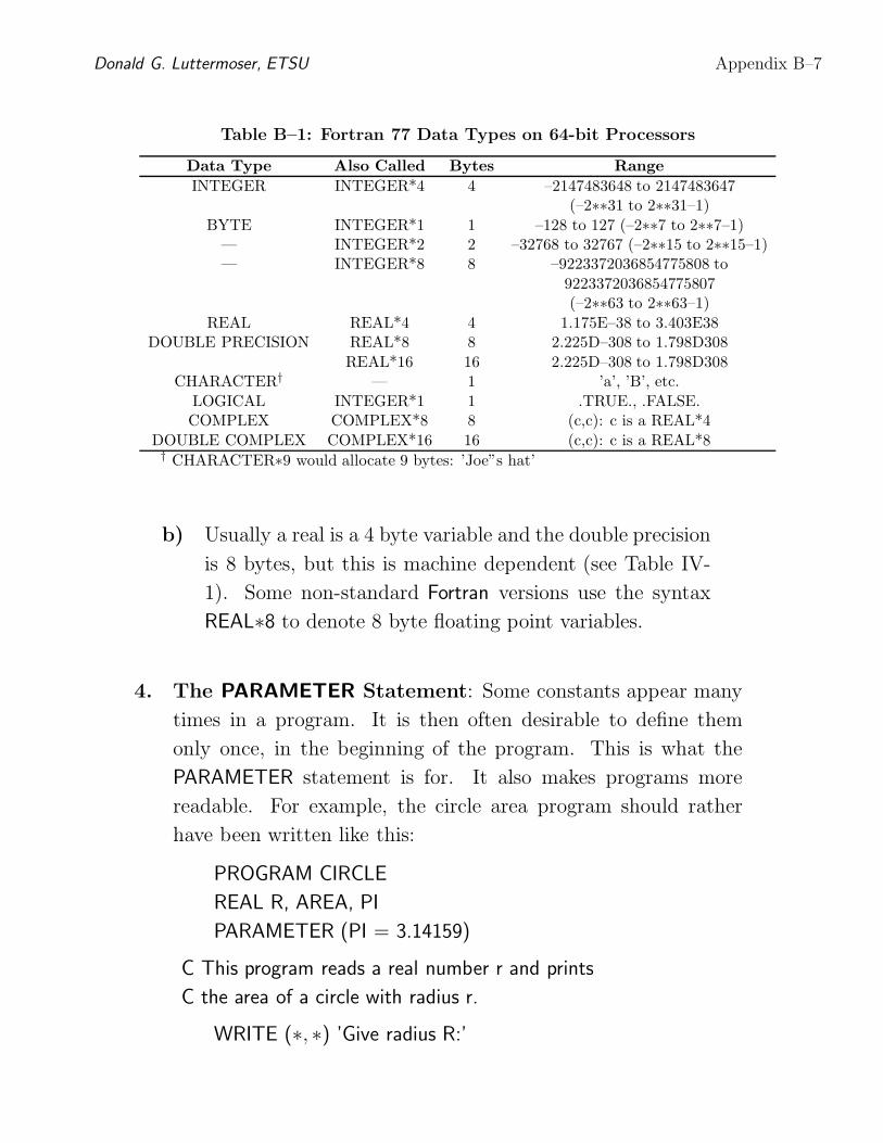
Table B–1: Fortran 77 Data Types on 64-bit Processors
Data Type Also Called Bytes Range
INTEGER INTEGER*4 4 –2147483648 to 2147483647(–2∗∗31 to 2∗∗31–1)
BYTE INTEGER*1 1 –128 to 127 (–2∗∗7 to 2∗∗7–1)— INTEGER*2 2 –32768 to 32767 (–2∗∗15 to 2∗∗15–1)— INTEGER*8 8 –9223372036854775808 to
9223372036854775807(–2∗∗63 to 2∗∗63–1)
REAL REAL*4 4 1.175E–38 to 3.403E38DOUBLE PRECISION REAL*8 8 2.225D–308 to 1.798D308
REAL*16 16 2.225D–308 to 1.798D308CHARACTER† — 1 ’a’, ’B’, etc.
LOGICAL INTEGER*1 1 .TRUE., .FALSE.COMPLEX COMPLEX*8 8 (c,c): c is a REAL*4
DOUBLE COMPLEX COMPLEX*16 16 (c,c): c is a REAL*8† CHARACTER∗9 would allocate 9 bytes: ’Joe”s hat’
b) Usually a real is a 4 byte variable and the double precision
is 8 bytes, but this is machine dependent (see Table IV-
1). Some non-standard Fortran versions use the syntax
REAL∗8 to denote 8 byte floating point variables.
4. The PARAMETER Statement: Some constants appear many
times in a program. It is then often desirable to define them
only once, in the beginning of the program. This is what the
PARAMETER statement is for. It also makes programs more
readable. For example, the circle area program should rather
have been written like this:
PROGRAM CIRCLE
REAL R, AREA, PI
PARAMETER (PI = 3.14159)
C This program reads a real number r and prints
C the area of a circle with radius r.
WRITE (∗, ∗) ’Give radius R:’
Appendix B–8 PHYS-4007/5007: Computational Physics
READ (∗, ∗) R
AREA = PI∗R∗R
WRITE (∗, ∗) ’Area = ’, AREA
STOP
END
a) The syntax of the parameter statement is
PARAMETER (name = constant, ... , name = constant )
b) The rules for the PARAMETER statement are:
i) The name defined in the PARAMETER statement
is not a variable but rather a constant. (You cannot
change its value at a later point in the program.)
ii) A name can appear in at most one PARAMETER
statement.
iii) The PARAMETER statement(s) must come be-
fore the first executable statement.
c) Some good reasons to use the PARAMETER statement
are:
i) It helps reduce the number of typos.
ii) It makes it easier to change a constant that ap-
pears many times in a program.
iii) It increases the readability of your program.
C. Fortran Expressions and Assignment.
1. Constants: The simplest form of an expression is a constant.
There are 6 types of constants, corresponding to the 6 data types:
a) Integers: 3, -606.
Donald G. Luttermoser, ETSU Appendix B–9
b) Reals: -2.345, 6.0234E-23.
c) Double precision constants: -2.34567823D-1, 1.0D209].
d) Complex: (2, -3), (1., 9.9E-1) — this is designated by a
pair of constants (integer or real), separated by a comma
and enclosed in parentheses, the first number denotes the
real part and the second the imaginary part.
e) Logical: .TRUE., .FALSE. — note that the dots are re-
quired.
f) Character constants: ’abc’, ’Hi There!’.
i) Strings and character constants are case sensitive.
A problem arises if you want to have an apostrophe
in the string itself.
ii) In this case, you should double the apostrophe:
’It”s a nice day’
2. Expressions: The simplest non-constant expressions are of the
form
operand operator operand
and an example is
X + Y
The result of an expression is itself an operand, hence we can
nest expressions together like X + 2 ∗ Y
a) This raises the question of precedence: Does the last ex-
pression mean X + (2∗Y) or (X+2)∗Y? The precedence
of arithmetic operators in Fortran 77 are (from highest to
lowest):
Appendix B–10 PHYS-4007/5007: Computational Physics
∗∗ exponentiation
∗, / multiplication, division+,− addition, subtraction
b) All these operators are calculated left-to-right, except the
exponentiation operator ∗∗, which has right-to-left prece-
dence.
c) If you want to change the default evaluation order, you
can use parentheses.
d) The above operators are all binary operators.
e) There is also the unary operator − for negation, which
takes precedence over the others. Hence an expression
like −X+Y means what you would expect.
f) Extreme caution must be taken when using the division
operator, which has a quite different meaning for integers
and reals.
i) If the operands are both integers, an integer divi-
sion is performed, otherwise a real arithmetic divi-
sion is performed.
ii) For example, 3/2 equals 1, while 3./2. equals 1.5
(note the decimal points).
3. Assignment: The assignment has the form
variable name = expression
The interpretation is as follows: Evaluate the right hand side
and assign the resulting value to the variable on the left. The
expression on the right may contain other variables, but these
Donald G. Luttermoser, ETSU Appendix B–11
never change value! For example,
AREA = PI ∗ R∗∗2
does not change the value of PI or R, only AREA.
4. Type Conversion: When different data types occur in the same
expression, type conversion has to take place, either explicitly or
implicitly.
a) Fortran will do some type conversion implicitly. For ex-
ample,
REAL X
X = X + 1
will convert the integer one to the real number one, and
has the desired effect of incrementing X by one.
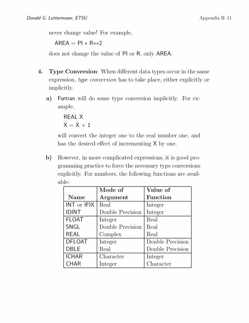
b) However, in more complicated expressions, it is good pro-
gramming practice to force the necessary type conversions
explicitly. For numbers, the following functions are avail-
able:
Mode of Value of
Name Argument Function
INT or IFIX Real Integer
IDINT Double Precision Integer
FLOAT Integer Real
SNGL Double Precision Real
REAL Complex Real
DFLOAT Integer Double Precision
DBLE Real Double Precision
ICHAR Character Integer
CHAR Integer Character
Appendix B–12 PHYS-4007/5007: Computational Physics
Example B–1. How to multiply two real variables X
and Y using double precision and store the result in the
double precision variable W:
W = DBLE(X)∗DBLE(Y)
Note that this is different from
W = DBLE(X∗Y)
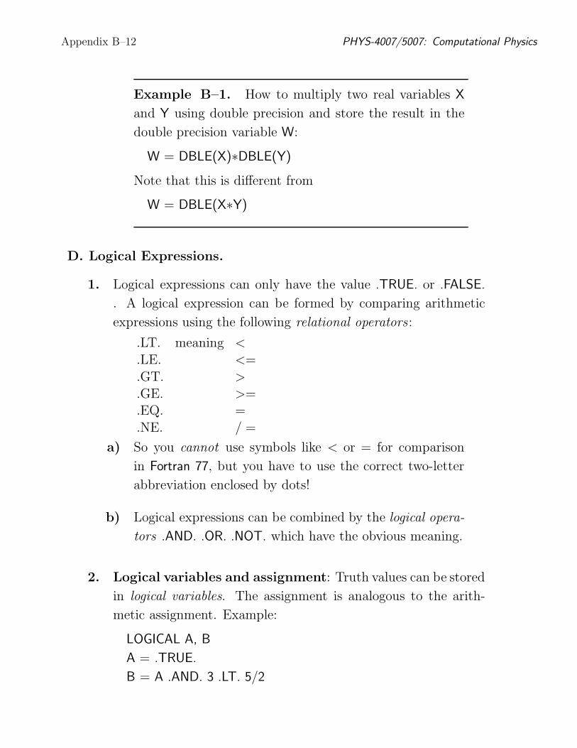
D. Logical Expressions.
1. Logical expressions can only have the value .TRUE. or .FALSE.
. A logical expression can be formed by comparing arithmetic
expressions using the following relational operators :
.LT. meaning <
.LE. <=
.GT. >
.GE. >=
.EQ. =
.NE. / =
a) So you cannot use symbols like < or = for comparison
in Fortran 77, but you have to use the correct two-letter
abbreviation enclosed by dots!
b) Logical expressions can be combined by the logical opera-
tors .AND. .OR. .NOT. which have the obvious meaning.
2. Logical variables and assignment: Truth values can be stored
in logical variables. The assignment is analogous to the arith-
metic assignment. Example:
LOGICAL A, B
A = .TRUE.
B = A .AND. 3 .LT. 5/2

Donald G. Luttermoser, ETSU Appendix B–13
a) The order of precedence is important, as the last example
shows. The rule is that arithmetic expressions are eval-
uated first, then relational operators, and finally logical
operators. Hence B will be assigned .FALSE. in the exam-
ple above.
b) Among the logical operators the precedence (in the ab-
sence of parenthesis) is that .NOT. is done first, then
.AND., then .OR. is done last.
c) Logical variables are seldom used in Fortran. But logical
expressions are frequently used in conditional statements
like the IF statement.
E. The IF Statements.
1. An important part of any programming language are the condi-
tional statements. The most common such statement in Fortran
is the IF statement, which actually has several forms. The sim-
plest one is the logical IF statement:
IF (logical expression ) executable statement
This has to be written on one line. This example finds the abso-
lute value of X:
IF (X .LT. 0) X = –X
a) If more than one statement should be executed inside the
IF, then the following syntax should be used:
IF (logical expression ) THEN
statements
ENDIF
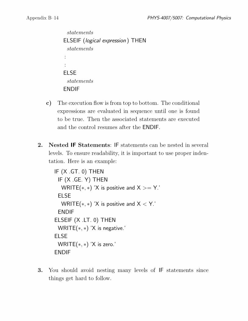
b) The most general form of the IF statement has the follow-
ing form:
IF (logical expression ) THEN
Appendix B–14 PHYS-4007/5007: Computational Physics
statements
ELSEIF (logical expression ) THEN
statements
:
:
ELSE
statements
ENDIF
c) The execution flow is from top to bottom. The conditional
expressions are evaluated in sequence until one is found
to be true. Then the associated statements are executed
and the control resumes after the ENDIF.
2. Nested IF Statements: IF statements can be nested in several
levels. To ensure readability, it is important to use proper inden-
tation. Here is an example:
IF (X .GT. 0) THEN
IF (X .GE. Y) THEN
WRITE(∗, ∗) ’X is positive and X >= Y.’
ELSE
WRITE(∗, ∗) ’X is positive and X < Y.’
ENDIF
ELSEIF (X .LT. 0) THEN
WRITE(∗, ∗) ’X is negative.’
ELSE
WRITE(∗, ∗) ’X is zero.’
ENDIF
3. You should avoid nesting many levels of IF statements since
things get hard to follow.

Donald G. Luttermoser, ETSU Appendix B–15
F. Fortran Loops.
1. For repeated execution of similar things, loops are used. Fortran
77 has only one loop construct, called the DO-loop. The DO-loop
corresponds to what is known as a for -loop in other languages.
Other loop constructs have to be built using the IF and GOTO
statements.
2. DO-Loops: The DO-loop is used for simple counting. Here is a
simple example that prints the cumulative sums of the integers
from 1 through N (assume N has been assigned a value else-
where):
INTEGER I, N, SUM
DO 10 I = 1, N
SUM = SUM + I
WRITE(∗, ∗) ’I = ’, I
WRITE(∗, ∗) ’SUM = ’, SUM
10 CONTINUE
a) The number 10 is a statement label. Typically, there will
be many loops and other statements in a single program
that require a statement label.
b) The programmer is responsible for assigning a unique num-
ber to each label in each program (or subprogram).
c) Recall that column positions 1-5 are reserved for state-
ment labels. The numerical value of statement labels have
no significance, so any integers can be used, in any order.
Typically, most programmers use consecutive multiples of
10.

Appendix B–16 PHYS-4007/5007: Computational Physics
3. The variable defined in the DO-statement is incremented by 1 by
default. However, you can define the step to be any number but
zero. This program segment prints the even numbers between 1
and 10 in decreasing order:
INTEGER I
DO 20 I = 10, 1, -2
WRITE(∗, ∗) ’I = ’, I
20 CONTINUE
4. The general form of the DO-loop is as follows:
DO label var = expr1, expr2, expr3
statements
label CONTINUE
a) var is the loop variable (often called the loop index ) which
must be integer.
b) expr1 specifies the initial value of var,
c) expr2 is the terminating bound,
d) expr3 is the increment (step).
e) Note: The DO-loop variable must never be changed by
other statements within the loop! This will cause great
confusion.
5. The loop index can be of type real, but due to round off errors
may not take on exactly the expected sequence of values. It’s
recommended that you use integers for the loop index.
6. Many Fortran 77 compilers allow DO-loops to be closed by the
ENDDO statement. The advantage of this is that the statement

Donald G. Luttermoser, ETSU Appendix B–17
label can then be omitted since it is assumed that an ENDDO
closes the nearest previous DO statement. The ENDDO construct
is widely used, but it is not a part of ANSI Fortran 77.
7. It should be noted that unlike some programming languages, For-
tran only evaluates the start, end, and step expressions once, be-
fore the first pass thought the body of the loop. This means that
the following DO-loop will multiply a non-negative J by two (the
hard way), rather than running forever as the equivalent loop
might in another language.
INTEGER I, J
READ(∗, ∗) J
DO I = 1, J
J = J + 1
ENDDO
WRITE(∗, ∗) J
8. While-Loops: The most intuitive way to write a WHILE-loop is
WHILE (logical expr) DO
statements
ENDDO
or alternatively,
DO WHILE (logical expr)
statements
ENDDO
a) The program will alternate testing the condition and exe-
cuting the statements in the body as long as the condition
in the WHILE statement is true.
b) Even though this syntax is accepted by many compilers,
it is not ANSI Fortran 77. The correct way is to use IF and

Appendix B–18 PHYS-4007/5007: Computational Physics
GOTO:
label IF (logical expr) THEN
statements
GOTO label
ENDIF
c) Here is an example that calculates and prints all the pow-
ers of two that are less than or equal to 100:
INTEGER N
N = 1
10 IF (N .LE. 100) THEN
WRITE(∗, ∗) N
N = 2∗N
GOTO 10
ENDIF
9. Until-Loops: If the termination criterion is at the end instead
of the beginning, it is often called an until-loop. The pseudocode
looks like this:
DO
statements
UNTIL (logical expr)
Again, this should be implemented in Fortran 77 by using IF and
GOTO:
label CONTINUE
statements
IF (logical expr) GOTO label
Note that the logical expression in the latter version should be
the negation of the expression given in the pseudocode!

Donald G. Luttermoser, ETSU Appendix B–19
G. Fortran Arrays.
1. Many scientific computations use vectors and matrices. The data
type Fortran uses for representing such objects is the array.
a) A one-dimensional array corresponds to a vector, while
a two-dimensional array corresponds to a matrix.
b) To fully understand how this works in Fortran 77, you will
have to know not only the syntax for usage, but also how
these objects are stored in memory.
2. One-dimensional arrays: The simplest array is the one-dimensional
array, which is just a sequence of elements stored consecutively
in memory.
a) For example, the declaration
REAL A(20)
declares A as a real array of length 20. That is, A consists
of 20 real numbers stored contiguously in memory.
b) By convention, Fortran arrays are indexed from 1 and up.
Thus the first number in the array is denoted by A(1) and
the last by A(20).
c) Note that this is different from either C and IDL, where a
20-dimensional array would range from A[0] to A[19].
d) However, in Fortran, it is possible to define an arbitrary
index range for your arrays using the following syntax:
REAL B(0:19), WEIRD(–162:237)
Here, B is exactly similar to A from the previous example,
except the index runs from 0 through 19. WEIRD is an
array of length 237–(–162)+1 = 400.
Appendix B–20 PHYS-4007/5007: Computational Physics
3. The type of an array element can be any of the basic data types.
Examples:
INTEGER I(10)
LOGICAL AA(0:1)
DOUBLE PRECISION X(100)
4. Each element of an array can be thought of as a separate variable.
You reference the I’th element of array A by A(I). Here is a code
segment that stores the 10 first square numbers in the array SQ:
INTEGER I, SQ(10)
DO 100 I = 1, 10
SQ(I) = I∗∗2
100 CONTINUE
5. A common bug in Fortran is that the program tries to access
array elements that are out of bounds or undefined. This is the
responsibility of the programmer, and the Fortran compiler will
not detect any such bugs prior to execution!
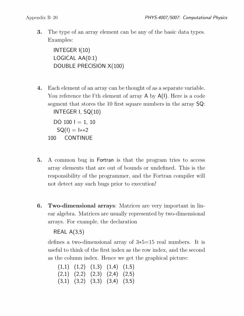
6. Two-dimensional arrays: Matrices are very important in lin-
ear algebra. Matrices are usually represented by two-dimensional
arrays. For example, the declaration
REAL A(3,5)
defines a two-dimensional array of 3∗5=15 real numbers. It is
useful to think of the first index as the row index, and the second
as the column index. Hence we get the graphical picture:
(1,1) (1,2) (1,3) (1,4) (1,5)
(2,1) (2,2) (2,3) (2,4) (2,5)(3,1) (3,2) (3,3) (3,4) (3,5)
Donald G. Luttermoser, ETSU Appendix B–21
7. Two-dimensional arrays may also have indices in an arbitrary
defined range. The general syntax for declarations is:
name (low index1 : hi index1, low index2 : hi index2)
The total size of the array is then
size = (hi index1-low index1+1)∗(hi index2-low index2+1)
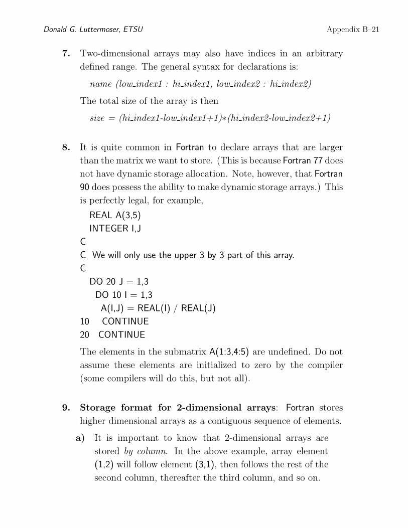
8. It is quite common in Fortran to declare arrays that are larger
than the matrix we want to store. (This is because Fortran 77 does
not have dynamic storage allocation. Note, however, that Fortran
90 does possess the ability to make dynamic storage arrays.) This
is perfectly legal, for example,
REAL A(3,5)
INTEGER I,J
C
C We will only use the upper 3 by 3 part of this array.
C
DO 20 J = 1,3
DO 10 I = 1,3
A(I,J) = REAL(I) / REAL(J)
10 CONTINUE
20 CONTINUE
The elements in the submatrix A(1:3,4:5) are undefined. Do not
assume these elements are initialized to zero by the compiler
(some compilers will do this, but not all).
9. Storage format for 2-dimensional arrays: Fortran stores
higher dimensional arrays as a contiguous sequence of elements.
a) It is important to know that 2-dimensional arrays are
stored by column. In the above example, array element
(1,2) will follow element (3,1), then follows the rest of the
second column, thereafter the third column, and so on.
Appendix B–22 PHYS-4007/5007: Computational Physics
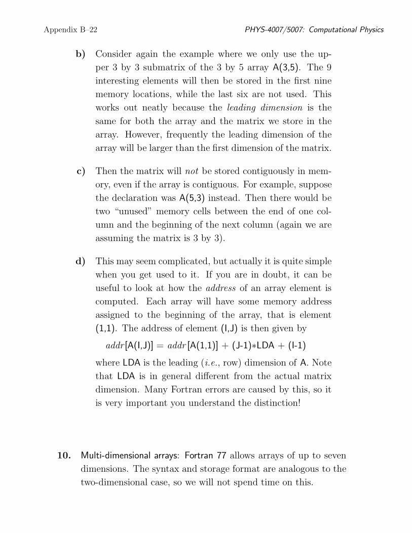
b) Consider again the example where we only use the up-
per 3 by 3 submatrix of the 3 by 5 array A(3,5). The 9
interesting elements will then be stored in the first nine
memory locations, while the last six are not used. This
works out neatly because the leading dimension is the
same for both the array and the matrix we store in the
array. However, frequently the leading dimension of the
array will be larger than the first dimension of the matrix.
c) Then the matrix will not be stored contiguously in mem-
ory, even if the array is contiguous. For example, suppose
the declaration was A(5,3) instead. Then there would be
two “unused” memory cells between the end of one col-
umn and the beginning of the next column (again we are
assuming the matrix is 3 by 3).
d) This may seem complicated, but actually it is quite simple
when you get used to it. If you are in doubt, it can be
useful to look at how the address of an array element is
computed. Each array will have some memory address
assigned to the beginning of the array, that is element
(1,1). The address of element (I,J) is then given by
addr [A(I,J)] = addr [A(1,1)] + (J-1)∗LDA + (I-1)
where LDA is the leading (i.e., row) dimension of A. Note
that LDA is in general different from the actual matrix
dimension. Many Fortran errors are caused by this, so it
is very important you understand the distinction!
10. Multi-dimensional arrays: Fortran 77 allows arrays of up to seven
dimensions. The syntax and storage format are analogous to the
two-dimensional case, so we will not spend time on this.

Donald G. Luttermoser, ETSU Appendix B–23
11. The DIMENSION Statement: There is an alternate way to
declare arrays in Fortran 77. The statements
REAL A, X
DIMENSION X(50)
DIMENSION A(10,20)
are equivalent to
REAL A(10,20), X(50)
This DIMENSION statement is considered old-fashioned style to-
day.
H. Fortran Subprograms.
1. When a program is more than a few hundred lines long, it gets
hard to follow. Fortran codes that solve real engineering and
scientific problems often have tens of thousands of lines. The
only way to handle such big codes, is to use a modular approach
and split the program into many separate smaller units called
subprograms.
a) A subprogram is a (small) piece of code that solves a well
defined subproblem. In a large program, one often has to
solve the same subproblems with many different data.
b) Instead of replicating code, these tasks should be solved
by subprograms.
c) The same subprogram can be invoked many times with
different input data.
d) Fortran has two different types of subprograms, called
functions and subroutines.
e) In C, all subprograms are functions, even the “main” pro-
gram is a function.

Appendix B–24 PHYS-4007/5007: Computational Physics
f) Meanwhile in IDL, the two types of subprograms are func-
tions (like Fortran functions) and procedures.
2. Functions: Fortran functions are quite similar to mathematical
functions: They both take a set of input arguments (parameters)
and return a value of some type.
a) In the preceding discussion we talked about user defined
subprograms. Fortran 77 also has some intrinsic (built-in)
functions.
b) A simple example illustrates how to use a function:
X = COS(PI/3.0)
Here COS is the cosine function, so X will be assigned the
value 0.5 (if PI has been correctly defined; Fortran 77 has
no built-in constants, unlike IDL which has !PI as a single-
precision constant of π and !DPI as the double-precision
version).
c) There are many intrinsic functions in Fortran 77. Some of
the most common are:
ABS absolute valueMIN minimum value
MAX maximum value
SQRT square root
SIN sineCOS cosine
TAN tangent
ATAN arctangentEXP exponential (natural)
LOG logarithm (natural)
d) In general, a function always has a type. Most of the
intrinsic functions mentioned above, however, are generic.

Donald G. Luttermoser, ETSU Appendix B–25
So in the example above, PI and X could be either of
type REAL or DOUBLE PRECISION. The compiler would
check the types and use the correct version of COS (real
or double precision).
e) Unfortunately, Fortran 77 is not really a polymorphic lan-
guage (unlike IDL which is) so in general you have to be
careful to match the types of your variables and your func-
tions! (See the Fortran Function Conversion handout on the
course web pages.)
3. Now we turn to the user-written functions. Consider the follow-
ing problem: A meteorologist has studied the precipitation levels
in the Bay Area and has come up with a model r(m, t), where r
is the amount of rain, m is the month, and t is a scalar parameter
that depends on the location. Given the formula for r and the
value of t, compute the annual rainfall.
a) The obvious way to solve the problem is to write a loop
that runs over all the months and sums up the values
of r. Since computing the value of r is an independent
subproblem, it is convenient to implement it as a function.
b) The following main program can be used:
PROGRAM RAIN
REAL R, T, SUM
INTEGER M
READ (∗, ∗) T
SUM = 0.0
DO 10 M = 1, 12
SUM = SUM + R(M,T)
10 CONTINUE
Appendix B–26 PHYS-4007/5007: Computational Physics
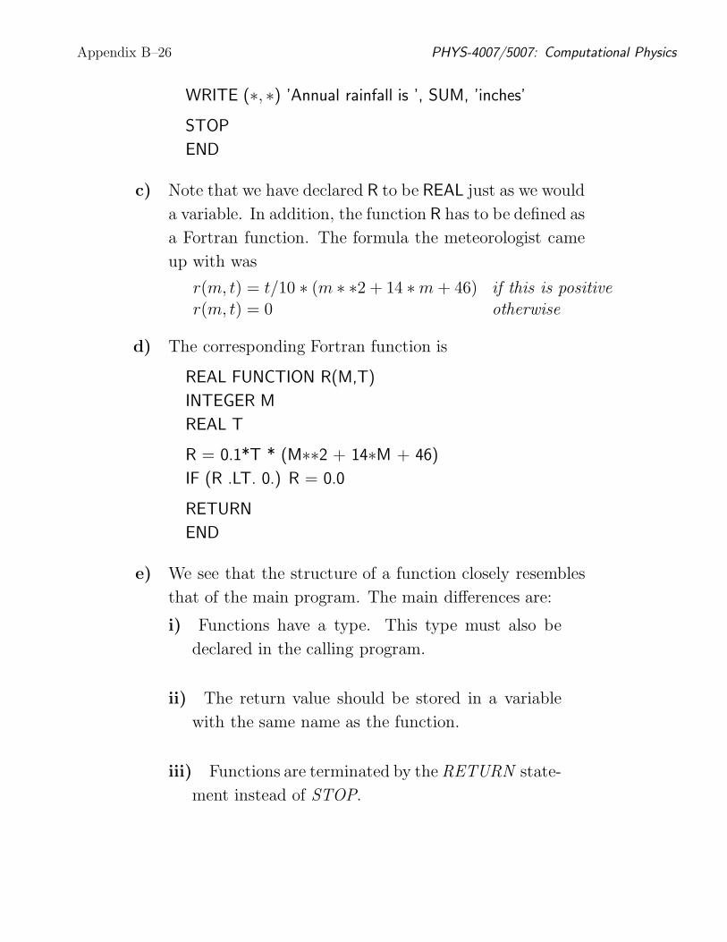
WRITE (∗, ∗) ’Annual rainfall is ’, SUM, ’inches’
STOP
END
c) Note that we have declared R to be REAL just as we would
a variable. In addition, the function R has to be defined as
a Fortran function. The formula the meteorologist came
up with was
r(m, t) = t/10 ∗ (m ∗ ∗2 + 14 ∗ m + 46) if this is positive
r(m, t) = 0 otherwise
d) The corresponding Fortran function is
REAL FUNCTION R(M,T)
INTEGER M
REAL T
R = 0.1*T * (M∗∗2 + 14∗M + 46)
IF (R .LT. 0.) R = 0.0
RETURN
END
e) We see that the structure of a function closely resembles
that of the main program. The main differences are:
i) Functions have a type. This type must also be
declared in the calling program.
ii) The return value should be stored in a variable
with the same name as the function.
iii) Functions are terminated by the RETURN state-
ment instead of STOP.

Donald G. Luttermoser, ETSU Appendix B–27
f) To sum up, the general syntax of a Fortran 77 function is:
type FUNCTION name (list-of-variables)
declarations
statements
RETURN
END
g) The function has to be declared with the correct type in
the calling program unit. If you use a function which has
not been declared, Fortran will try to use the same implicit
typing used for variables, probably getting it wrong.
h) The function is called by simply using the function name
and listing the parameters in parenthesis.
i) It should be noted that strictly speaking Fortran 77 doesn’t
permit recursion (functions which call themselves). How-
ever, it is not uncommon for a compiler to allow recursion.
4. Subroutines: A Fortran function can essentially only return one
value. Often we want to return two or more values (or sometimes
none!). For this purpose we use the SUBROUTINE construct.
The syntax is as follows:
SUBROUTINE name (list-of-arguments)
declarations
statements
RETURN
END
a) Note that subroutines have no type and consequently should
not (cannot) be declared in the calling program unit.
b) They are also invoked differently than functions, using the
word CALL before their names and parameters.

Appendix B–28 PHYS-4007/5007: Computational Physics
c) We give an example of a very simple subroutine. The
purpose of the subroutine is to swap two integers.
SUBROUTINE ISWAP(A,B)
INTEGER A, B
C Local variables
INTEGER TMP
TMP = A
A = B
B = TMP
RETURN
END
d) Note that there are two blocks of variable declarations
here. First, we declare the input/output parameters, i.e.,
the variables that are common to both the caller and the
callee. Afterwards, we declare the local variables, i.e., the
variables that can only be used within this subprogram.
e) We can use the same variable names in different subpro-
grams and the compiler will know that they are different
variables that just happen to have the same names.
5. Call-by-reference: Fortran 77 uses the so-called call-by-reference
paradigm.
a) This means that instead of just passing the values of the
function/subroutine arguments (call-by-value ), the mem-
ory address of the arguments (pointers) are passed in-
stead. A small example should show the difference:
PROGRAM CALLEX
INTEGER M, N
C
M = 1
Donald G. Luttermoser, ETSU Appendix B–29
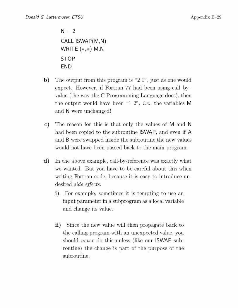
N = 2
CALL ISWAP(M,N)
WRITE (∗, ∗) M,N
STOP
END
b) The output from this program is “2 1”, just as one would
expect. However, if Fortran 77 had been using call–by–
value (the way the C Programming Language does), then
the output would have been “1 2”, i.e., the variables M
and N were unchanged!
c) The reason for this is that only the values of M and N
had been copied to the subroutine ISWAP, and even if A
and B were swapped inside the subroutine the new values
would not have been passed back to the main program.
d) In the above example, call-by-reference was exactly what
we wanted. But you have to be careful about this when
writing Fortran code, because it is easy to introduce un-
desired side effects.
i) For example, sometimes it is tempting to use an
input parameter in a subprogram as a local variable
and change its value.
ii) Since the new value will then propagate back to
the calling program with an unexpected value, you
should never do this unless (like our ISWAP sub-
routine) the change is part of the purpose of the
subroutine.

Appendix B–30 PHYS-4007/5007: Computational Physics
6. We will come back to this issue in a later section on passing
arrays as arguments (parameters).
I. Arrays in Subprograms.
1. Fortran subprogram calls are based on call-by-reference. This
means that the calling parameters are not copied to the called
subprogram, but rather that the addresses of the parameters
(variables) are passed.
a) This saves a lot of memory space when dealing with ar-
rays. No extra storage is needed as the subroutine oper-
ates on the same memory locations as the calling
(sub-)program.
b) However, you as a programmer have to know about this
and take it into account.
c) It is possible to declare local arrays in Fortran subpro-
grams, but this feature is rarely used. Typically, all arrays
are declared (and dimensioned) in the main program and
then passed on to the subprograms as needed.
2. Variable length arrays: A basic vector operation is the SAXPY
operation. This calculates the expression
y = α ∗ x + y
where α is a scalar but x and y are vectors. Here is a simple
subroutine for this:
SUBROUTINE SAXPY(ALPHA, X, Y, N)
INTEGER N
REAL ALPHA, X(∗), Y(∗)
C
C SAXPY: Compute y = alpha∗x + y,
C where x and y are vectors of length n (at least).
Donald G. Luttermoser, ETSU Appendix B–31
C
C Local variables
INTEGER I
C
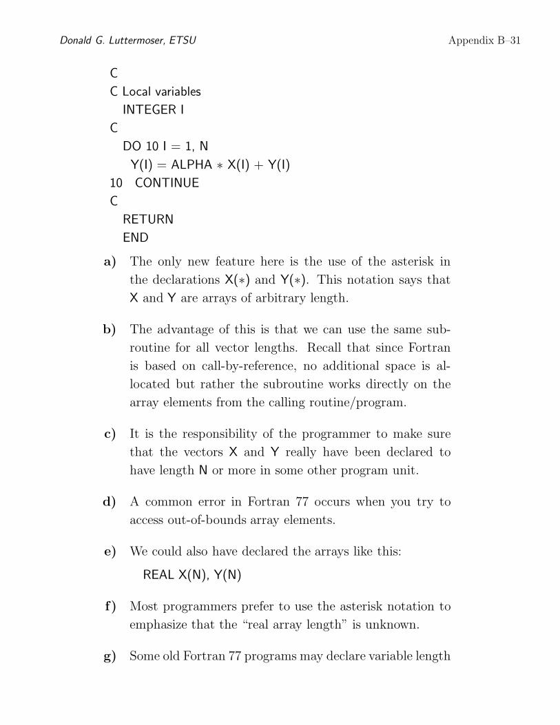
DO 10 I = 1, N
Y(I) = ALPHA ∗ X(I) + Y(I)
10 CONTINUE
C
RETURN
END
a) The only new feature here is the use of the asterisk in
the declarations X(∗) and Y(∗). This notation says that
X and Y are arrays of arbitrary length.
b) The advantage of this is that we can use the same sub-
routine for all vector lengths. Recall that since Fortran
is based on call-by-reference, no additional space is al-
located but rather the subroutine works directly on the
array elements from the calling routine/program.
c) It is the responsibility of the programmer to make sure
that the vectors X and Y really have been declared to
have length N or more in some other program unit.
d) A common error in Fortran 77 occurs when you try to
access out-of-bounds array elements.
e) We could also have declared the arrays like this:
REAL X(N), Y(N)
f) Most programmers prefer to use the asterisk notation to
emphasize that the “real array length” is unknown.
g) Some old Fortran 77 programs may declare variable length
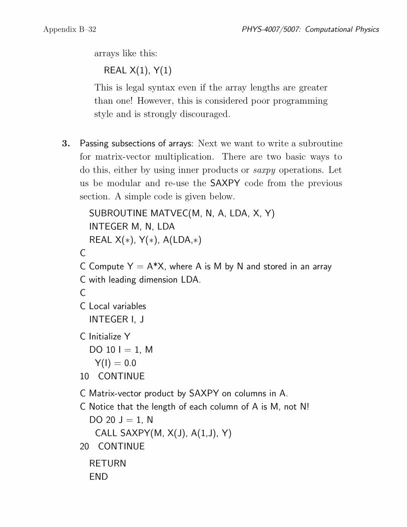
Appendix B–32 PHYS-4007/5007: Computational Physics
arrays like this:
REAL X(1), Y(1)
This is legal syntax even if the array lengths are greater
than one! However, this is considered poor programming
style and is strongly discouraged.
3. Passing subsections of arrays: Next we want to write a subroutine
for matrix-vector multiplication. There are two basic ways to
do this, either by using inner products or saxpy operations. Let
us be modular and re-use the SAXPY code from the previous
section. A simple code is given below.
SUBROUTINE MATVEC(M, N, A, LDA, X, Y)
INTEGER M, N, LDA
REAL X(∗), Y(∗), A(LDA,∗)
C
C Compute Y = A*X, where A is M by N and stored in an array
C with leading dimension LDA.
C
C Local variables
INTEGER I, J
C Initialize Y
DO 10 I = 1, M
Y(I) = 0.0
10 CONTINUE
C Matrix-vector product by SAXPY on columns in A.
C Notice that the length of each column of A is M, not N!
DO 20 J = 1, N
CALL SAXPY(M, X(J), A(1,J), Y)
20 CONTINUE
RETURN
END

Donald G. Luttermoser, ETSU Appendix B–33
a) There are several important things to note here. First,
note that even if we have written the code as general as
possible to allow for arbitrary dimensions M and N, we
still need to specify the leading dimension of the matrix
A.
b) The variable length declaration (∗) can only be used for
the last dimension of an array! The reason for this is the
way Fortran 77 stores multidimensional arrays (see the
section on arrays, §H in this Appendix).
c) When we compute y = A∗x by saxpy operations, we need
to access columns of A. The J’th column of A is A(1:M,J).
However, in Fortran 77 we cannot use such subarray syn-
tax (but it is encouraged in Fortran 90!).
d) So instead we provide a pointer to the first element in the
column, which is A(1,J) (it is not really a pointer, but it
may be helpful to think of it as if it were). We know that
the next memory locations will contain the succeeding
array elements in this column. The SAXPY subroutine
will treat A(1,J) as the first element of a vector, and does
not know that this vector happens to be a column of a
matrix.
e) Finally, note that we have stuck to the convention that
matrices have M rows and N columns. The index I is used
as a row index (1 to M), while the index J is used as a
column index (1 to N). Most Fortran programs handling
linear algebra use this notation and it makes it a lot easier
to read the code!
Appendix B–34 PHYS-4007/5007: Computational Physics
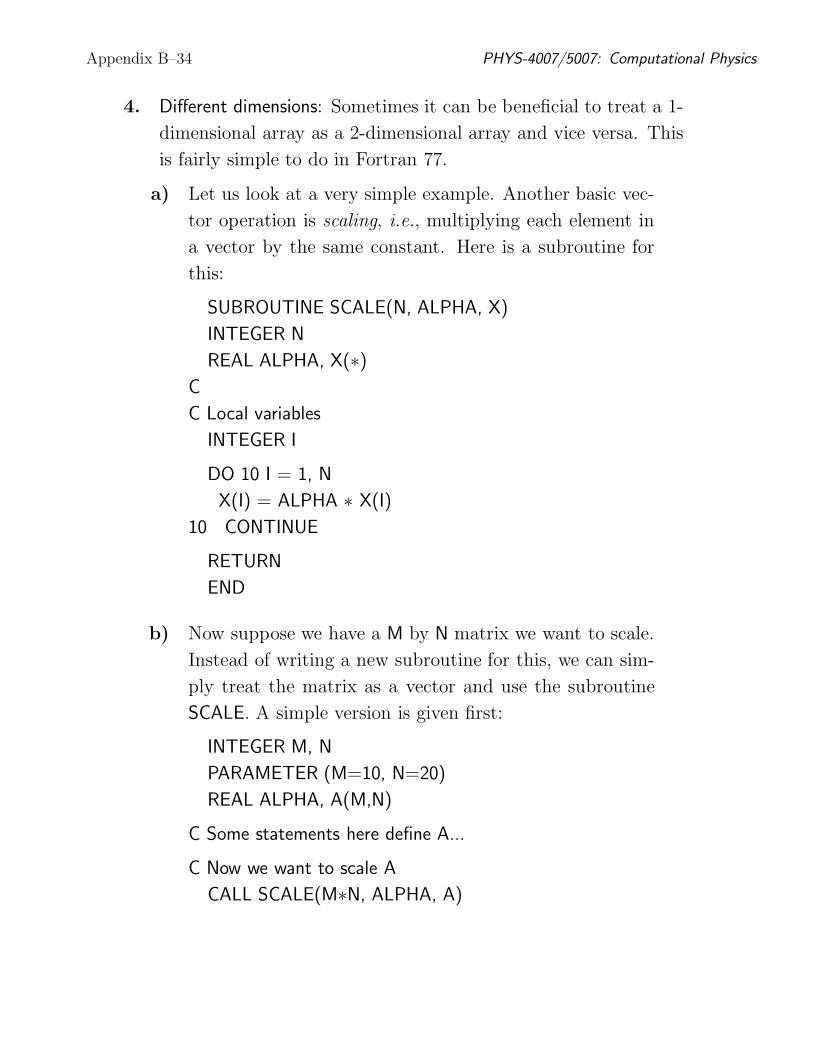
4. Different dimensions: Sometimes it can be beneficial to treat a 1-
dimensional array as a 2-dimensional array and vice versa. This
is fairly simple to do in Fortran 77.
a) Let us look at a very simple example. Another basic vec-
tor operation is scaling, i.e., multiplying each element in
a vector by the same constant. Here is a subroutine for
this:
SUBROUTINE SCALE(N, ALPHA, X)
INTEGER N
REAL ALPHA, X(∗)
C
C Local variables
INTEGER I
DO 10 I = 1, N
X(I) = ALPHA ∗ X(I)
10 CONTINUE
RETURN
END
b) Now suppose we have a M by N matrix we want to scale.
Instead of writing a new subroutine for this, we can sim-
ply treat the matrix as a vector and use the subroutine
SCALE. A simple version is given first:
INTEGER M, N
PARAMETER (M=10, N=20)
REAL ALPHA, A(M,N)
C Some statements here define A...
C Now we want to scale A
CALL SCALE(M∗N, ALPHA, A)
Donald G. Luttermoser, ETSU Appendix B–35
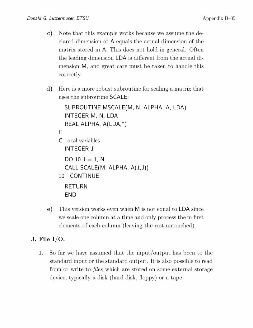
c) Note that this example works because we assume the de-
clared dimension of A equals the actual dimension of the
matrix stored in A. This does not hold in general. Often
the leading dimension LDA is different from the actual di-
mension M, and great care must be taken to handle this
correctly.
d) Here is a more robust subroutine for scaling a matrix that
uses the subroutine SCALE:
SUBROUTINE MSCALE(M, N, ALPHA, A, LDA)
INTEGER M, N, LDA
REAL ALPHA, A(LDA,*)
C
C Local variables
INTEGER J
DO 10 J = 1, N
CALL SCALE(M, ALPHA, A(1,J))
10 CONTINUE
RETURN
END
e) This version works even when M is not equal to LDA since
we scale one column at a time and only process the m first
elements of each column (leaving the rest untouched).
J. File I/O.
1. So far we have assumed that the input/output has been to the
standard input or the standard output. It is also possible to read
from or write to files which are stored on some external storage
device, typically a disk (hard disk, floppy) or a tape.

Appendix B–36 PHYS-4007/5007: Computational Physics
2. In Fortran each file is associated with a unit number, an integer
between 1 and 99 (IDL also follows the Fortran style). Some unit
numbers are reserved: 5 is standard input, 6 is standard output.
3. Opening and closing a file: Before you can use a file you have
to open it. The command is
OPEN (list-of-specifiers )
where the most common specifiers are:
UNIT = u
IOSTAT = iosERR = err
FILE = fname
STATUS = staACCESS = acc
FORM = frm
RECL = rl
a) The unit number u is a number in the range 1-99 that
denotes this file (the programmer may chose any number
but he/she has to make sure it is unique).
b) ios is the I/O status identifier and should be an integer
variable. Upon return, ios is zero if the statement was
successful and returns a non-zero value otherwise.
c) err is a label which the program will jump to if there is
an error.
d) fname is a character string denoting the file name.
e) sta is a character string that has to be either NEW, OLD
or SCRATCH. It shows the prior status of the file. A
scratch file is a file that is created when opened and deleted
when closed (or the program ends).
Donald G. Luttermoser, ETSU Appendix B–37
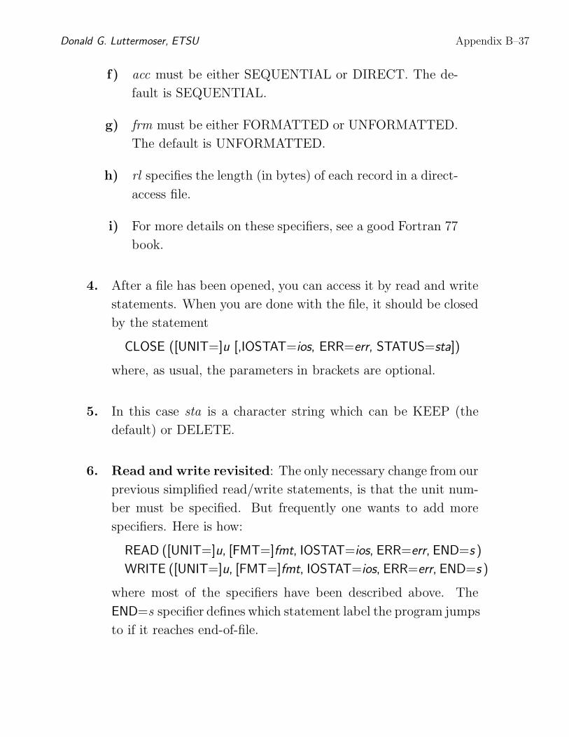
f) acc must be either SEQUENTIAL or DIRECT. The de-
fault is SEQUENTIAL.
g) frm must be either FORMATTED or UNFORMATTED.
The default is UNFORMATTED.
h) rl specifies the length (in bytes) of each record in a direct-
access file.
i) For more details on these specifiers, see a good Fortran 77
book.
4. After a file has been opened, you can access it by read and write
statements. When you are done with the file, it should be closed
by the statement
CLOSE ([UNIT=]u [,IOSTAT=ios, ERR=err, STATUS=sta])
where, as usual, the parameters in brackets are optional.
5. In this case sta is a character string which can be KEEP (the
default) or DELETE.
6. Read and write revisited: The only necessary change from our
previous simplified read/write statements, is that the unit num-
ber must be specified. But frequently one wants to add more
specifiers. Here is how:
READ ([UNIT=]u, [FMT=]fmt, IOSTAT=ios, ERR=err, END=s )
WRITE ([UNIT=]u, [FMT=]fmt, IOSTAT=ios, ERR=err, END=s )
where most of the specifiers have been described above. The
END=s specifier defines which statement label the program jumps
to if it reaches end-of-file.
Appendix B–38 PHYS-4007/5007: Computational Physics
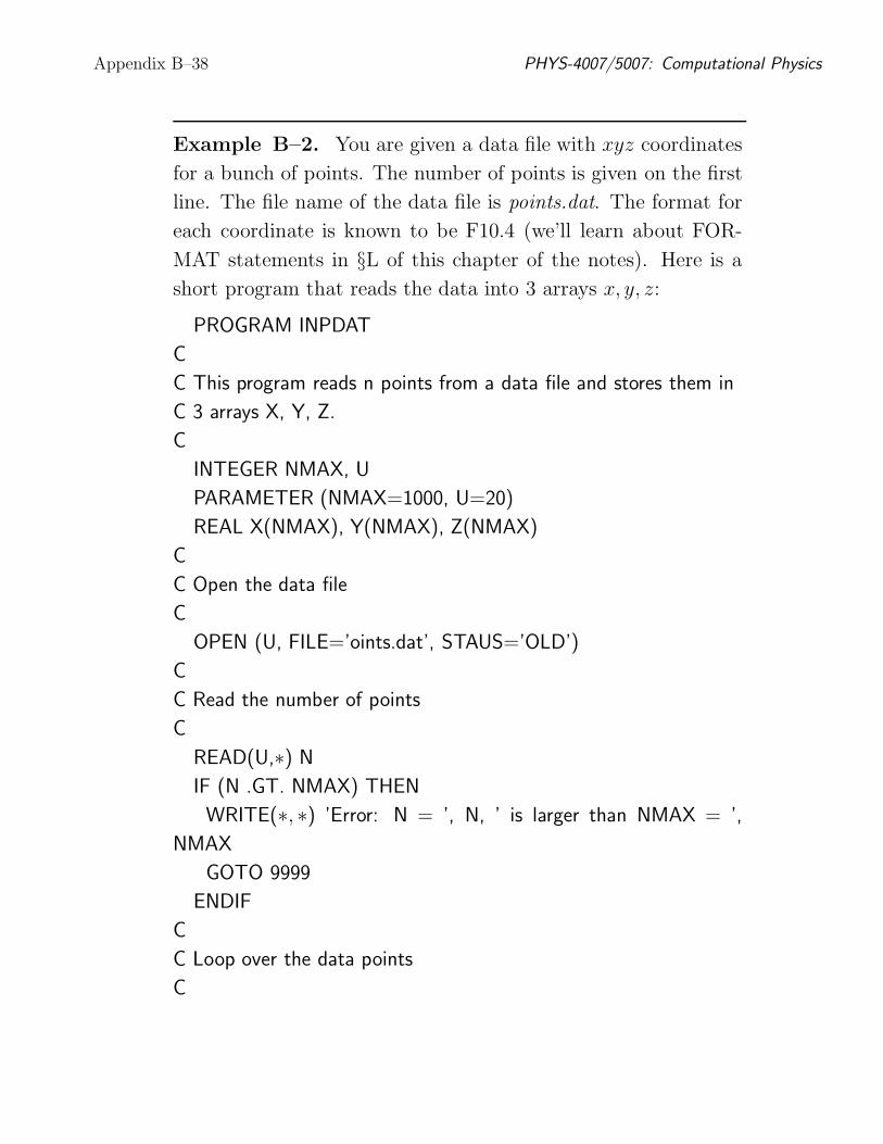
Example B–2. You are given a data file with xyz coordinates
for a bunch of points. The number of points is given on the first
line. The file name of the data file is points.dat. The format for
each coordinate is known to be F10.4 (we’ll learn about FOR-
MAT statements in §L of this chapter of the notes). Here is a
short program that reads the data into 3 arrays x, y, z:
PROGRAM INPDAT
C
C This program reads n points from a data file and stores them in
C 3 arrays X, Y, Z.
C
INTEGER NMAX, U
PARAMETER (NMAX=1000, U=20)
REAL X(NMAX), Y(NMAX), Z(NMAX)
C
C Open the data file
C
OPEN (U, FILE=’oints.dat’, STAUS=’OLD’)
C
C Read the number of points
C
READ(U,∗) N
IF (N .GT. NMAX) THEN
WRITE(∗, ∗) ’Error: N = ’, N, ’ is larger than NMAX = ’,
NMAX
GOTO 9999
ENDIF
C
C Loop over the data points
C
Donald G. Luttermoser, ETSU Appendix B–39
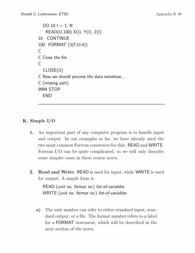
DO 10 I = 1, N
READ(U,100) X(I), Y(I), Z(I)
10 CONTINUE
100 FORMAT (3(F10.4))
C
C Close the file
C
CLOSE(U)
C Now we should process the data somehow...
C (missing part)
9999 STOP
END
K. Simple I/O
1. An important part of any computer program is to handle input
and output. In our examples so far, we have already used the
two most common Fortran constructs for this: READ and WRITE.
Fortran I/O can be quite complicated, so we will only describe
some simpler cases in these course notes.
2. Read and Write: READ is used for input, while WRITE is used
for output. A simple form is
READ (unit no, format no ) list-of-variables
WRITE (unit no, format no ) list-of-variables
a) The unit number can refer to either standard input, stan-
dard output, or a file. The format number refers to a label
for a FORMAT statement, which will be described in the
next section of the notes.

Appendix B–40 PHYS-4007/5007: Computational Physics
b) It is possible to simplify these statements further by using
asterisks (∗) for some arguments, like we have done in
most of our examples so far. This is sometimes called list
directed read/write.
READ (∗, ∗) list-of-variables
WRITE (∗, ∗) list-of-variables
c) The first statement will read values from the standard
input and assign the values to the variables in the variable
list, while the second one writes to the standard output.
Example B–3. Here is a code segment from a Fortran pro-
gram:
INTEGER M, N
REAL X, Y, Z(10)
READ(∗, ∗) M, N
READ(∗, ∗) X, Y
READ (∗, ∗) Z
We give the input through standard input (possibly through a
data file directed to standard input). A data file consists of
records according to traditional Fortran terminology. In this ex-
ample, each record contains a number (either integer or real).
Records are separated by either blanks or commas. Hence a le-
gal input to the program above would be:
–1 100
–1.0 1e+2
1.0 2.0 3.0 4.0 5.0 6.0 7.0 8.0 9.0 10.0
Or, we could add commas as separators:
–1, 100
–1.0, 1E+2
1.0, 2.0, 3.0, 4.0, 5.0, 6.0, 7.0, 8.0, 9.0, 10.0

Donald G. Luttermoser, ETSU Appendix B–41
3. Note that Fortran 77 input is line sensitive, so it is important
not to have extra input elements (fields) on a line (record). For
example, if we gave the first four inputs all on one line as
–1 100, –1.0, 1E+2
1.0, 2.0, 3.0, 4.0, 5.0, 6.0, 7.0, 8.0, 9.0, 10.0
then M and N would be assigned the values –1 and 100 respec-
tively, but the last two values would be discarded, X and Y would
be assigned the values 1.0 and 2.0, ignoring the rest of the second
line. This would leave the elements of Z all undefined.
4. If there are too few inputs on a line then the next line will be
read. For example
–1
100
–1.0
1E+2
1.0, 2.0, 3.0, 4.0, 5.0, 6.0, 7.0, 8.0, 9.0, 10.0
would produce the same results as the first two examples.
5. Other versions: For simple list-directed I/O it is possible to
use the alternate syntax
READ ∗, list-of-variables
PRINT ∗, list-of-variables
which has the same meaning as the list-directed read and write
statements described earlier. This version always reads/writes to
standard input/output so the ∗ corresponds to the format.
L. Format Statements.
1. So far we have mostly used free format input/output. This uses a
set of default rules for how to input and output values of different
Appendix B–42 PHYS-4007/5007: Computational Physics
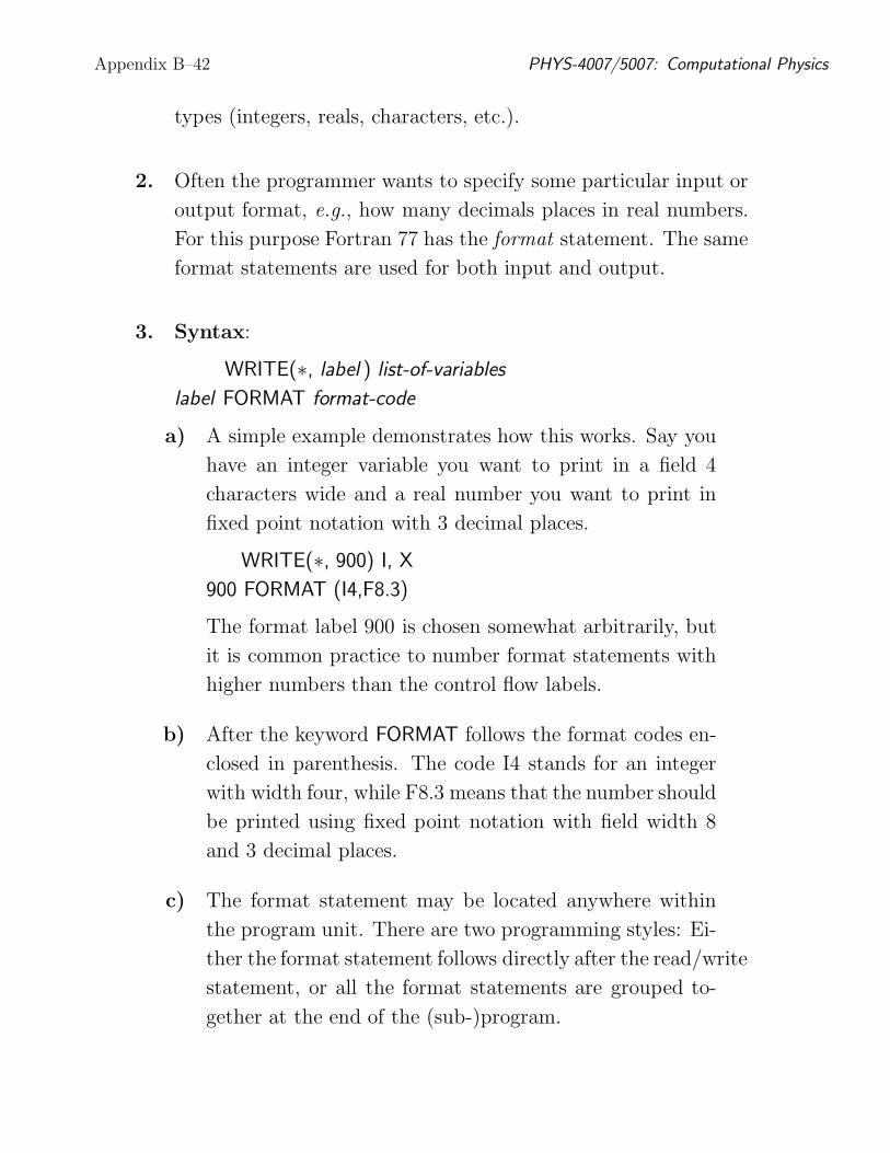
types (integers, reals, characters, etc.).
2. Often the programmer wants to specify some particular input or
output format, e.g., how many decimals places in real numbers.
For this purpose Fortran 77 has the format statement. The same
format statements are used for both input and output.
3. Syntax:
WRITE(∗, label ) list-of-variables
label FORMAT format-code
a) A simple example demonstrates how this works. Say you
have an integer variable you want to print in a field 4
characters wide and a real number you want to print in
fixed point notation with 3 decimal places.
WRITE(∗, 900) I, X
900 FORMAT (I4,F8.3)
The format label 900 is chosen somewhat arbitrarily, but
it is common practice to number format statements with
higher numbers than the control flow labels.
b) After the keyword FORMAT follows the format codes en-
closed in parenthesis. The code I4 stands for an integer
with width four, while F8.3 means that the number should
be printed using fixed point notation with field width 8
and 3 decimal places.
c) The format statement may be located anywhere within
the program unit. There are two programming styles: Ei-
ther the format statement follows directly after the read/write
statement, or all the format statements are grouped to-
gether at the end of the (sub-)program.
Donald G. Luttermoser, ETSU Appendix B–43
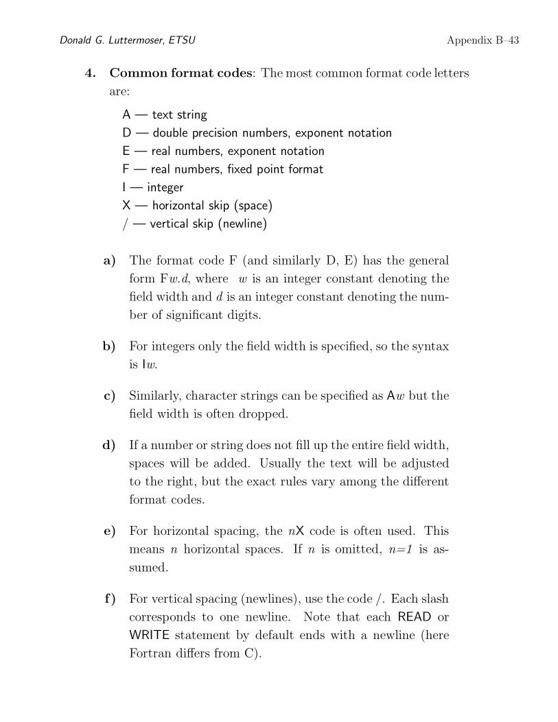
4. Common format codes: The most common format code letters
are:
A — text string
D — double precision numbers, exponent notation
E — real numbers, exponent notation
F — real numbers, fixed point format
I — integer
X — horizontal skip (space)
/ — vertical skip (newline)
a) The format code F (and similarly D, E) has the general
form Fw.d, where w is an integer constant denoting the
field width and d is an integer constant denoting the num-
ber of significant digits.
b) For integers only the field width is specified, so the syntax
is Iw.
c) Similarly, character strings can be specified as Aw but the
field width is often dropped.
d) If a number or string does not fill up the entire field width,
spaces will be added. Usually the text will be adjusted
to the right, but the exact rules vary among the different
format codes.
e) For horizontal spacing, the nX code is often used. This
means n horizontal spaces. If n is omitted, n=1 is as-
sumed.
f) For vertical spacing (newlines), use the code /. Each slash
corresponds to one newline. Note that each READ or
WRITE statement by default ends with a newline (here
Fortran differs from C).
Appendix B–44 PHYS-4007/5007: Computational Physics
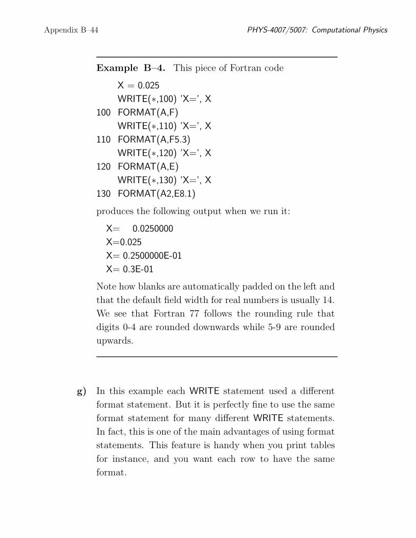
Example B–4. This piece of Fortran code
X = 0.025
WRITE(∗,100) ’X=’, X
100 FORMAT(A,F)
WRITE(∗,110) ’X=’, X
110 FORMAT(A,F5.3)
WRITE(∗,120) ’X=’, X
120 FORMAT(A,E)
WRITE(∗,130) ’X=’, X
130 FORMAT(A2,E8.1)
produces the following output when we run it:
X= 0.0250000
X=0.025
X= 0.2500000E-01
X= 0.3E-01
Note how blanks are automatically padded on the left and
that the default field width for real numbers is usually 14.
We see that Fortran 77 follows the rounding rule that
digits 0-4 are rounded downwards while 5-9 are rounded
upwards.
g) In this example each WRITE statement used a different
format statement. But it is perfectly fine to use the same
format statement for many different WRITE statements.
In fact, this is one of the main advantages of using format
statements. This feature is handy when you print tables
for instance, and you want each row to have the same
format.

Donald G. Luttermoser, ETSU Appendix B–45
5. Format strings in READ/WRITE statements: Instead of
specifying the format code in a separate format statement, one
can give the format code in the READ/WRITE statement directly.
For example, the statement
WRITE (∗,’(A, F8.3)’) ’The answer is X = ’, X
is equivalent to
WRITE (∗,990) ’The answer is X = ’, X
990 FORMAT (A,F8.3)
Sometimes text strings are given in the format statements, e.g.,
the following version is also equivalent:
WRITE (∗,999) X
999 FORMAT (’The answer is x = ’,F8.3)
6. Implicit loops and repeat counts: Now let us do a more
complicated example. Say you have a two-dimensional array of
integers and want to print the upper left 5 by 10 submatrix with
10 values each on 5 rows. Here is how:
DO 10 I = 1, 5
WRITE(∗,1000) (A(I,J), J=1,10)
10 CONTINUE
1000 FORMAT (I6)
a) We have an explicit do loop over the rows and an implicit
loop over the column index J.
b) Often a format statement involves repetition, for example
950 FORMAT (2X, I3, 2X, I3, 2X, I3, 2X, I3)
There is a shorthand notation for this:
950 FORMAT (4(2X, I3))
c) It is also possible to allow repetition without explicitly
stating how many times the format should be repeated.
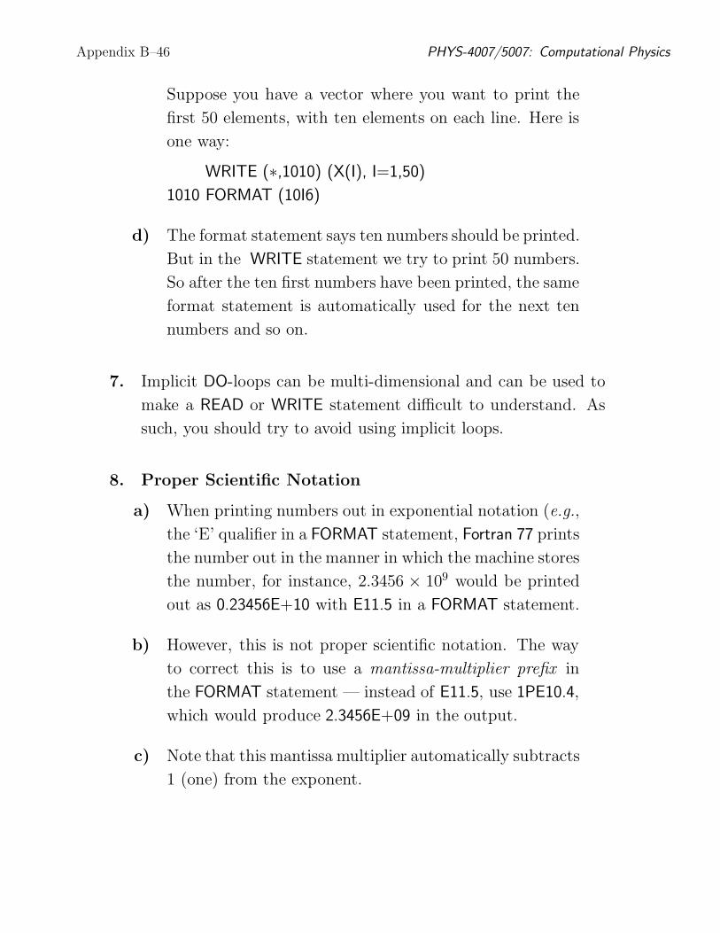
Appendix B–46 PHYS-4007/5007: Computational Physics
Suppose you have a vector where you want to print the
first 50 elements, with ten elements on each line. Here is
one way:
WRITE (∗,1010) (X(I), I=1,50)
1010 FORMAT (10I6)
d) The format statement says ten numbers should be printed.
But in the WRITE statement we try to print 50 numbers.
So after the ten first numbers have been printed, the same
format statement is automatically used for the next ten
numbers and so on.
7. Implicit DO-loops can be multi-dimensional and can be used to
make a READ or WRITE statement difficult to understand. As
such, you should try to avoid using implicit loops.
8. Proper Scientific Notation
a) When printing numbers out in exponential notation (e.g.,
the ‘E’ qualifier in a FORMAT statement, Fortran 77 prints
the number out in the manner in which the machine stores
the number, for instance, 2.3456 × 10⁹ would be printed
out as 0.23456E+10 with E11.5 in a FORMAT statement.
b) However, this is not proper scientific notation. The way
to correct this is to use a mantissa-multiplier prefix in
the FORMAT statement — instead of E11.5, use 1PE10.4,
which would produce 2.3456E+09 in the output.
c) Note that this mantissa multiplier automatically subtracts
1 (one) from the exponent.

Donald G. Luttermoser, ETSU Appendix B–47
d) This mantissa multiplier is applied to all floating point
numbers in the FORMAT statement after it is first used,
hence the ‘1P’ prefix would only have to be used once
in a given FORMAT statement, for instance, if IGH =
3458, R67 = 2.3456× 10⁹, I89 = 87, J67 = 19, and R98 =
−4.115645 × 10⁻⁷ in the WRITE statement below:
WRITE(12, 990) IGH, R67, I89, J67, R98
990 FORMAT(3X, I4, 1PE10.4, 2I3, E13.6)
would produce the following output:
3458 2.3456E+09 87 19 -4.115645E-07
e) However, this mantissa multiplier would also be used in
any floating-point number printed in decimal notation fol-
lowing its first use in a FORMAT statement. As such, if
YUH = 98.245 and DGL98 = -897.22 in the WRITE state-
ment below:
WRITE(12, 992) IGH, YUH, R67, R98, DGL98
992 FORMAT(3X, I4, F7.3, 1PE10.4, E13.6, F8.2)
This would produce the following output:
3458 98.245 2.3456E+09 -4.115645E-07 -8972.20
f) To fix this, we have to undo the mantissa multiplier with
the with the ‘0P’ (zero-P) format prefix, for instance in
the statement above:
WRITE(12, 992) IGH, YUH, R67, R98, DGL98
992 FORMAT(3X, I4, F7.3, 1PE10.4, E13.6, 0PF8.2)
This would produce the correct output:
3458 98.245 2.3456E+09 -4.115645E-07 -897.22
g) Note that if we had another variable to print in scientific
notation after the ‘0P’ prefix was issued in a FORMAT

Appendix B–48 PHYS-4007/5007: Computational Physics
statement, we would then have to include another ‘1P’
prefix after the ‘0P’ prefix was used, for instance:
WRITE(12, 992) IGH, YUH, R67, DGL98, R98
992 FORMAT(3X, I4, F7.3, 1PE10.4, 0PF8.2, 1PE13.6)
which would produce the correct output:
3458 98.245 2.3456E+09 -897.22 -4.115645E-07
h) Finally note that if we had a series of numbers to print in
scientific notation on one line, we would have the follow
FORMAT statement:
WRITE(12, 992) IGH, YUH, R67, DGL98, R98
992 FORMAT(3X, I4, F7.3, 1P3E10.4)
This would produce the following output:
3458 98.245 2.3456E+09 -8.9722E+02 -4.1156E-07
M. Common Blocks.
1. Fortran 77 has no global variables, i.e., variables that are shared
among several program units (subroutines).
2. The only way to pass information between subroutines we have
seen so far is to use the subroutine parameter list.
a) Sometimes this is inconvenient, e.g., when many subrou-
tines share a large set of parameters.
b) In such cases one can use a common block. This is a way
to specify that certain variables should be shared among
certain subroutines.
c) IDL also has common blocks. C, however, does not, but
instead, has global variables.
Donald G. Luttermoser, ETSU Appendix B–49
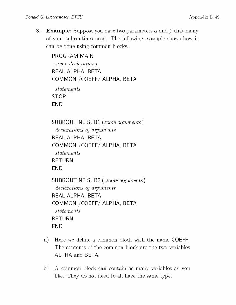
3. Example: Suppose you have two parameters α and β that many
of your subroutines need. The following example shows how it
can be done using common blocks.
PROGRAM MAIN
some declarations
REAL ALPHA, BETA
COMMON /COEFF/ ALPHA, BETA
statements
STOP
END
SUBROUTINE SUB1 (some arguments )
declarations of arguments
REAL ALPHA, BETA
COMMON /COEFF/ ALPHA, BETA
statements
RETURN
END
SUBROUTINE SUB2 ( some arguments )
declarations of arguments
REAL ALPHA, BETA
COMMON /COEFF/ ALPHA, BETA
statements
RETURN
END
a) Here we define a common block with the name COEFF.
The contents of the common block are the two variables
ALPHA and BETA.
b) A common block can contain as many variables as you
like. They do not need to all have the same type.
Appendix B–50 PHYS-4007/5007: Computational Physics
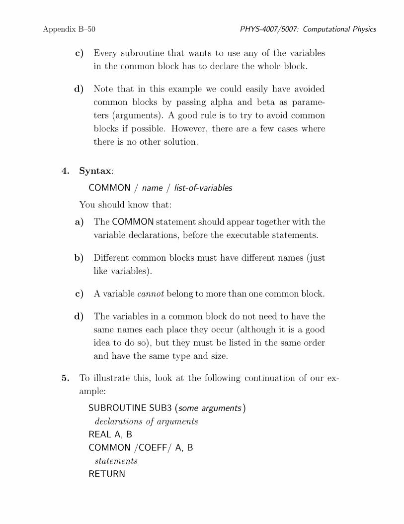
c) Every subroutine that wants to use any of the variables
in the common block has to declare the whole block.
d) Note that in this example we could easily have avoided
common blocks by passing alpha and beta as parame-
ters (arguments). A good rule is to try to avoid common
blocks if possible. However, there are a few cases where
there is no other solution.
4. Syntax:
COMMON / name / list-of-variables
You should know that:
a) The COMMON statement should appear together with the
variable declarations, before the executable statements.
b) Different common blocks must have different names (just
like variables).
c) A variable cannot belong to more than one common block.
d) The variables in a common block do not need to have the
same names each place they occur (although it is a good
idea to do so), but they must be listed in the same order
and have the same type and size.
5. To illustrate this, look at the following continuation of our ex-
ample:
SUBROUTINE SUB3 (some arguments )
declarations of arguments
REAL A, B
COMMON /COEFF/ A, B
statements
RETURN
Donald G. Luttermoser, ETSU Appendix B–51
END
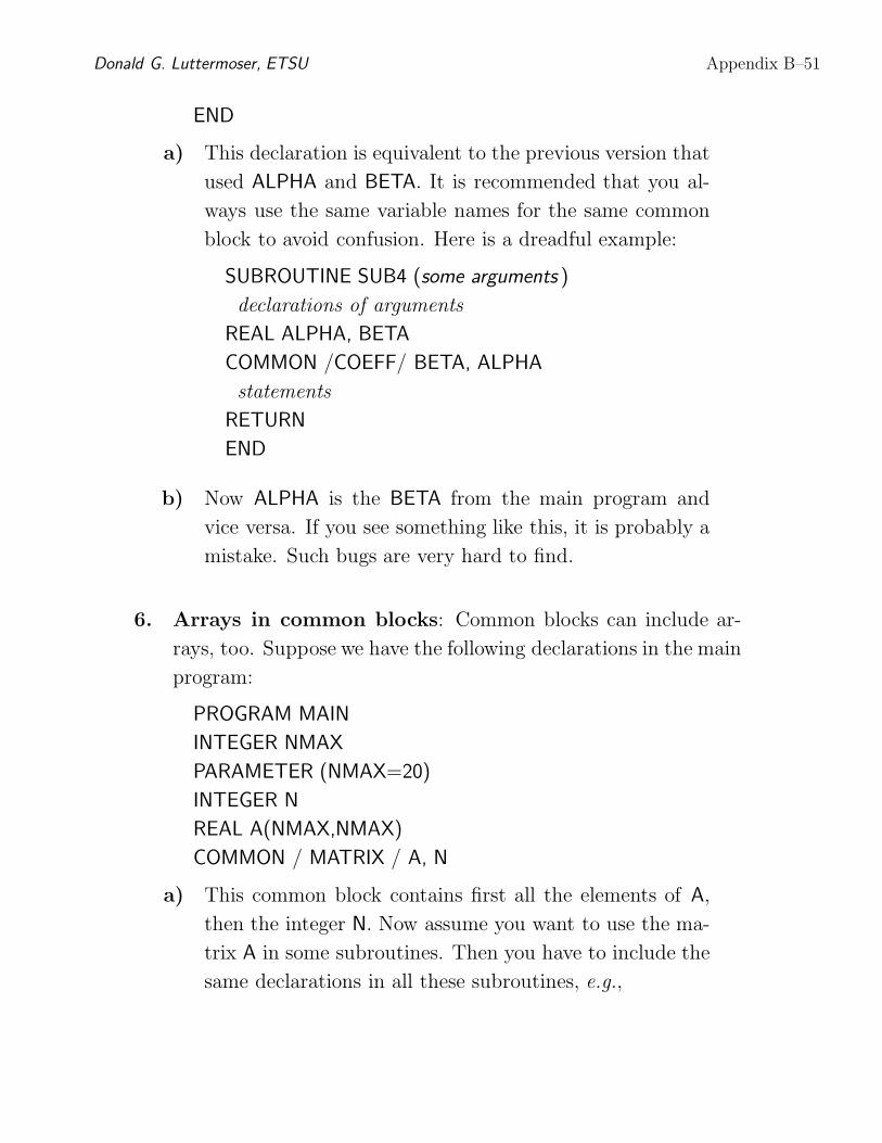
a) This declaration is equivalent to the previous version that
used ALPHA and BETA. It is recommended that you al-
ways use the same variable names for the same common
block to avoid confusion. Here is a dreadful example:
SUBROUTINE SUB4 (some arguments )
declarations of arguments
REAL ALPHA, BETA
COMMON /COEFF/ BETA, ALPHA
statements
RETURN
END
b) Now ALPHA is the BETA from the main program and
vice versa. If you see something like this, it is probably a
mistake. Such bugs are very hard to find.
6. Arrays in common blocks: Common blocks can include ar-
rays, too. Suppose we have the following declarations in the main
program:
PROGRAM MAIN
INTEGER NMAX
PARAMETER (NMAX=20)
INTEGER N
REAL A(NMAX,NMAX)
COMMON / MATRIX / A, N
a) This common block contains first all the elements of A,
then the integer N. Now assume you want to use the ma-
trix A in some subroutines. Then you have to include the
same declarations in all these subroutines, e.g.,
Appendix B–52 PHYS-4007/5007: Computational Physics
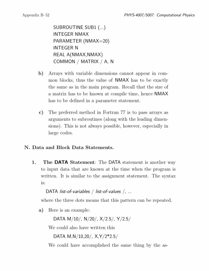
SUBROUTINE SUB1 (...)
INTEGER NMAX
PARAMETER (NMAX=20)
INTEGER N
REAL A(NMAX,NMAX)
COMMON / MATRIX / A, N
b) Arrays with variable dimensions cannot appear in com-
mon blocks, thus the value of NMAX has to be exactly
the same as in the main program. Recall that the size of
a matrix has to be known at compile time, hence NMAX
has to be defined in a parameter statement.
c) The preferred method in Fortran 77 is to pass arrays as
arguments to subroutines (along with the leading dimen-
sions). This is not always possible, however, especially in
large codes.
N. Data and Block Data Statements.
1. The DATA Statement: The DATA statement is another way
to input data that are known at the time when the program is
written. It is similar to the assignment statement. The syntax
is:
DATA list-of-variables / list-of-values /, ...
where the three dots means that this pattern can be repeated.
a) Here is an example:
DATA M/10/, N/20/, X/2.5/, Y/2.5/
We could also have written this
DATA M,N/10,20/, X,Y/2*2.5/
We could have accomplished the same thing by the as-

Donald G. Luttermoser, ETSU Appendix B–53
signments
M = 10
N = 20
X = 2.5
Y = 2.5
b) The DATA statement is more compact and therefore often
more convenient. Notice especially the shorthand nota-
tion for assigning identical values repeatedly.
c) The DATA statement is performed only once, right before
the execution of the program starts. For this reason, the
DATA statement is mainly used in the main program and
not in subroutines.
d) The DATA statement can also be used to initialize arrays
(vectors, matrices). This example shows how to make sure
a matrix is all zeros when the program starts:
REAL A(10,20)
DATA A/ 200 ∗ 0.0 /
e) Some compilers will automatically initialize arrays like
this but not all, so if you rely on array elements to be
zero it is a good idea to follow this example. Of course
you can initialize arrays to other values than zero. You
may even initialize individual elements:
DATA A(1,1)/12.5/, A(2,1)/–33.3/, A(2,2)/1.0/
Or you can list all the elements for small arrays like this:
INTEGER V(5)
REAL B(2,2)
DATA V/10,20,30,40,50/, B/1.0,-3.7,4.3,0.0/
Appendix B–54 PHYS-4007/5007: Computational Physics
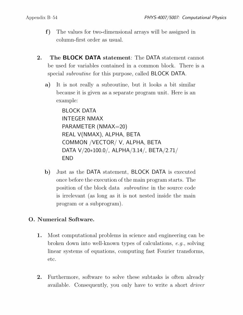
f) The values for two-dimensional arrays will be assigned in
column-first order as usual.
2. The BLOCK DATA statement: The DATA statement cannot
be used for variables contained in a common block. There is a
special subroutine for this purpose, called BLOCK DATA.
a) It is not really a subroutine, but it looks a bit similar
because it is given as a separate program unit. Here is an
example:
BLOCK DATA
INTEGER NMAX
PARAMETER (NMAX=20)
REAL V(NMAX), ALPHA, BETA
COMMON /VECTOR/ V, ALPHA, BETA
DATA V/20∗100.0/, ALPHA/3.14/, BETA/2.71/
END
b) Just as the DATA statement, BLOCK DATA is executed
once before the execution of the main program starts. The
position of the block data subroutine in the source code
is irrelevant (as long as it is not nested inside the main
program or a subprogram).
O. Numerical Software.
1. Most computational problems in science and engineering can be
broken down into well-known types of calculations, e.g., solving
linear systems of equations, computing fast Fourier transforms,
etc.
2. Furthermore, software to solve these subtasks is often already
available. Consequently, you only have to write a short driver
Donald G. Luttermoser, ETSU Appendix B–55
routine for your particular problem. This way people don’t have
to reinvent the wheel over and over again.
3. The best software for a particular type of problem must often be
purchased from a commercial company, but for linear algebra and
some other basic numerical computations there is high-quality
free software available (through Netlib).
4. Netlib: Netlib (the NET LIBrary) is a large collection of freely
available software, documents, and databases of interest to the
numerical, scientific computing, and other communities. The
repository is maintained by AT&T Bell Laboratories, the Uni-
versity of Tennessee and Oak Ridge National Laboratory, and
replicated at several sites around the world.
a) Netlib contains high-quality software that has been exten-
sively tested, but (as all free software) it comes with no
warranty and little (if any) support. In order to use the
software, you first have to download it to your computer
and then compile it yourself.
b) There are many ways to access Netlib. The most common
way is through their web page at
http://www.netlib.org/index.html
c) Two of the most popular packages at Netlib are the BLAS
and LAPACK libraries which we will describe in later sec-
tions.
5. Some commercial Fortran packages: In this section we briefly
mention a few of the largest (commercial) software packages for
general numerical computations.
Appendix B–56 PHYS-4007/5007: Computational Physics
a) NAG: The Numerical Algorithms Group (see
http://www.nag.com:81/) has developed a numerical
libraries at
http://www.nag.com:81/numeric/numerical libraries.asp
which are written in a variety of different programming
languages including Fortran. The Fortran library contains
over 1000 user-callable subroutines for solving general ap-
plied math problems, including: ordinary and partial dif-
ferential equations, optimization problems, FFT and other
transforms, quadrature, linear algebra, non-linear equa-
tions, integral equations, and more.
b) IMSL: The IMSL Fortran numerical library was origi-
nally sold by Visual Numerics, Inc., but now is sold by
Rogue Wave Software (http://www.roguewave.com/). The
IMSL software covers most of the areas contained in the
NAG library. It also has support for analyzing and pre-
senting statistical data in scientific and business applica-
tions.
c) Numerical Recipes: The books Numerical Recipes in
C/Fortran are very popular among scientists and engi-
neers because they can be used as a cookbooks where you
can find a recipe to solve the problem at hand. However,
the corresponding software is in no way (e.g., scope or
quality) comparable to that provided by NAG or IMSL.
d) It should be mentioned that all the software listed above
also comes in a C version (or is at least callable from C)
and other programming languages.

Donald G. Luttermoser, ETSU Appendix B–57
6. BLAS: BLAS is an acronym for Basic Linear Algebra Subrou-
tines. As the name indicates, it contains subprograms for basic
operations on vectors and matrices. BLAS was designed to be
used as a building block in other codes, for example LAPACK.
The source code for BLAS is available through Netlib. How-
ever, many computer vendors will have a special version of BLAS
tuned for maximal speed and efficiency on their computer. This
is one of the main advantages of BLAS: the calling sequences are
standardized so that programs that call BLAS will work on any
computer that has BLAS installed. If you have a fast version of
BLAS, you will also get high performance on all programs that
call BLAS. Hence BLAS provides a simple and portable way to
achieve high performance for calculations involving linear alge-
bra.
7. LAPACK is a higher-level package built on the same ideas.
8. Levels and naming conventions: The BLAS subroutines can
be divided into three levels :
a) Level 1: Vector-vector operations. O(n) data and O(n)
work.
b) Level 2: Matrix-vector operations. O(n2) data and O(n2)
work.
c) Level 3: Matrix-matrix operations. O(n2) data and O(n3)
work.
9. Each BLAS and LAPACK routine comes in several versions, one
for each precision (data type). The first letter of the subprogram
name indicates the precision used:

Appendix B–58 PHYS-4007/5007: Computational Physics
S Real single precision.
D Real double precision.C Complex single precision.
Z Complex double precision.
10. Complex double precision is not strictly defined in Fortran 77,
but most compilers will accept one of the following declarations:
DOUBLE COMPLEX list-of-variables
COMPLEX*16 list-of-variables
11. Elements of BLAS and How to Get It.
a) BLAS 1: Some of the BLAS 1 subprograms are:
xCOPY — copy one vector to anotherxSWAP — swap two vectors
xSCAL — scale a vector by a constant
xAXPY — add a multiple of one vector to anotherxDOT — inner product
xASUM — 1-norm of a vector
xNRM2 — 2-norm of a vector
IxAMAX — find maximal entry in a vector
The first letter (x) can be any of the letters S,D,C,Z de-
pending on the precision. A quick reference to BLAS 1
can be found at http://www.netlib.org/blas/blasqr.ps .
b) BLAS 2: Some of the BLAS 2 subprograms are:
xGEMV — general matrix-vector multiplicationxGER — general rank-1 update
xSYR2 — symmetric rank-2 update
xTRSV — solve a triangular system of equations
A detailed description of BLAS 2 can be found at
http://www.netlib.org/blas/blas2-paper.ps .
Donald G. Luttermoser, ETSU Appendix B–59
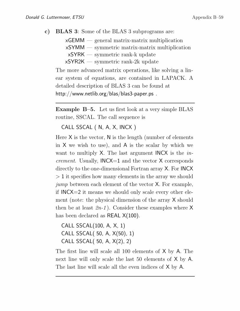
c) BLAS 3: Some of the BLAS 3 subprograms are:
xGEMM — general matrix-matrix multiplication
xSYMM — symmetric matrix-matrix multiplication
xSYRK — symmetric rank-k update
xSYR2K — symmetric rank-2k update
The more advanced matrix operations, like solving a lin-
ear system of equations, are contained in LAPACK. A
detailed description of BLAS 3 can be found at
http://www.netlib.org/blas/blas3-paper.ps .
Example B–5. Let us first look at a very simple BLAS
routine, SSCAL. The call sequence is
CALL SSCAL ( N, A, X, INCX )
Here X is the vector, N is the length (number of elements
in X we wish to use), and A is the scalar by which we
want to multiply X. The last argument INCX is the in-
crement. Usually, INCX=1 and the vector X corresponds
directly to the one-dimensional Fortran array X. For INCX
> 1 it specifies how many elements in the array we should
jump between each element of the vector X. For example,
if INCX=2 it means we should only scale every other ele-
ment (note: the physical dimension of the array X should
then be at least 2n-1 ). Consider these examples where X
has been declared as REAL X(100).
CALL SSCAL(100, A, X, 1)
CALL SSCAL( 50, A, X(50), 1)
CALL SSCAL( 50, A, X(2), 2)
The first line will scale all 100 elements of X by A. The
next line will only scale the last 50 elements of X by A.
The last line will scale all the even indices of X by A.

Appendix B–60 PHYS-4007/5007: Computational Physics
d) Observe that the array X will be overwritten by the new
values. If you need to preserve a copy of the old X, you
have to make a copy first, e.g., by using SCOPY.
e) Now consider a more complicated example. Suppose you
have two 2-dimensional arrays A and B, and you are asked
to find the (i, j) entry of the product A∗B.
i) This is easily done by computing the inner product
of row i from A and column j of B. We can use the
BLAS 1 subroutine SDOT. The only difficulty is to
figure out the correct indices and increments.
ii) The call sequence for SDOT is
CALL SDOT ( N, X, INCX, Y, INCY )
iii) Suppose the array declarations were
REAL A(LDA,LDA)
REAL B(LDB,LDB)
but in the program you know that the actual size
of A is M∗P and for B it is P∗N. The i’th row
of A starts at the element A(I,1). But since For-
tran stores 2-dimensional arrays down columns, the
next row element A(I,2) will be stored LDA elements
later in memory (since LDA is the length of a col-
umn). Hence we set INCX = LDA.
iv) For the column in B there is no such problem,
the elements are stored consecutively so INCY = 1.
The length of the inner product calculation is P.
Hence the answer is

Donald G. Luttermoser, ETSU Appendix B–61
CALL SDOT ( P, A(I,1), LDA, B(1,J), 1 )
f) How to get the BLAS: You can find it on Netlib at
http://www.netlib.org/blas/ .
g) Documentation: The BLAS routines are almost self-
explanatory. Once you know which routine you need,
fetch it and read the header section that explains the input
and output parameters in detail. We will look at an ex-
ample in the next section when we address the LAPACK
routines.
12. Elements of LAPACK and How to Get It.
a) LAPACK: LAPACK is a collection of Fortran subpro-
grams for advanced linear algebra problems like solving
systems of simultaneous linear equations, least-squares
solutions of linear systems of equations, eigenvalue prob-
lems, and singular value problems. LAPACK replaces the
older packages LINPACK and EISPACK. LAPACK sub-
routines were written to exploit BLAS as much as possi-
ble.
i) Routines: Probably the most widely used LA-
PACK routines are the ones that solve systems of
linear equations:
xGESV — Solve AX=B for a general matrix A
xPOSV — Solve AX=B for a symmetric positive
definite matrix AxGBSV — Solve AX=B for a general banded
matrix A
ii) There are many more routines for other special
types of matrices.

Appendix B–62 PHYS-4007/5007: Computational Physics
iii) The source code and executables for some com-
puters are available from Netlib at
http://www.netlib.org/lapack .
b) Documentation: Just like the BLAS routines, the LA-
PACK routines are virtually self-explanatory. Details of
the input and output parameters for any given subroutine
are contained in the header section of the file.
i) For example, here is the header section of the LA-PACK subroutine SGESV:
SUBROUTINE SGESV(N, NRHS, A, LDA, IPIV, B, LDB, INFO)∗
∗ – LAPACK driver routine (version 2.0) –∗ Univ. of Tennessee, Univ. of California Berkeley, NAG Ltd.,
∗ Courant Institute, Argonne National Lab, and Rice University∗ March 31, 1993
∗
∗ .. Scalar Arguments ..
INTEGER INFO, LDA, LDB, N, NRHS∗ ..
∗ .. Array Arguments ..INTEGER IPIV( ast )REAL A( LDA, ast ), B( LDB, ast )
∗ ..∗
∗ Purpose∗ =======
∗
∗ SGESV computes the solution to a real system of linear equations
∗ A ast X = B,∗ where A is an N-by-N matrix and X and B are N-by-NRHS
∗ matrices.∗
∗ The LU decomposition with partial pivoting and row interchanges
∗ is used to factor A as∗ A = P ast L ast U,
∗ where P is a permutation matrix, L is unit lower triangular, and U∗ is upper triangular. The factored form of A is then used to solve
∗ the system of equations A ast X = B.∗
∗ Arguments∗ =========
∗
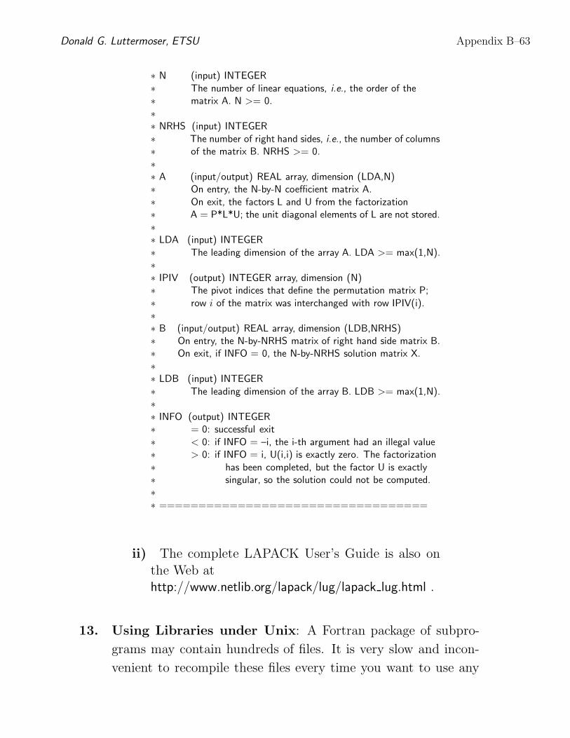
Donald G. Luttermoser, ETSU Appendix B–63
∗ N (input) INTEGER
∗ The number of linear equations, i.e., the order of the∗ matrix A. N >= 0.
∗
∗ NRHS (input) INTEGER
∗ The number of right hand sides, i.e., the number of columns∗ of the matrix B. NRHS >= 0.
∗
∗ A (input/output) REAL array, dimension (LDA,N)∗ On entry, the N-by-N coefficient matrix A.
∗ On exit, the factors L and U from the factorization∗ A = P*L*U; the unit diagonal elements of L are not stored.
∗
∗ LDA (input) INTEGER
∗ The leading dimension of the array A. LDA >= max(1,N).∗
∗ IPIV (output) INTEGER array, dimension (N)∗ The pivot indices that define the permutation matrix P;
∗ row i of the matrix was interchanged with row IPIV(i).∗
∗ B (input/output) REAL array, dimension (LDB,NRHS)∗ On entry, the N-by-NRHS matrix of right hand side matrix B.∗ On exit, if INFO = 0, the N-by-NRHS solution matrix X.
∗
∗ LDB (input) INTEGER
∗ The leading dimension of the array B. LDB >= max(1,N).∗
∗ INFO (output) INTEGER∗ = 0: successful exit
∗ < 0: if INFO = –i, the i-th argument had an illegal value∗ > 0: if INFO = i, U(i,i) is exactly zero. The factorization
∗ has been completed, but the factor U is exactly∗ singular, so the solution could not be computed.∗
∗ ==================================
ii) The complete LAPACK User’s Guide is also on
the Web athttp://www.netlib.org/lapack/lug/lapack lug.html .
13. Using Libraries under Unix: A Fortran package of subpro-
grams may contain hundreds of files. It is very slow and incon-
venient to recompile these files every time you want to use any
Appendix B–64 PHYS-4007/5007: Computational Physics
of the subroutines.
a) Under the Unix operating system you can avoid this by
making a library file. The library file is an object file, so
you only have to compile your additional main (driver)
program and then link it with library. (Linking is much
faster than compiling.)
b) Libraries have file names starting with lib and ending in
.a (and sometimes .so).
c) Currently, no Fortran math libraries have been installed
on the Linux side of the PCs in Brown Hall 264.
d) For a generic Unix system, if for example, the BLAS
library is stored in the file /usr/local/lib/libblas.a, you
would use the –l option to link it together with your main
program, e.g.,
f77 main.f –lblas
(note that on Linux, one would use the GNU Fortran com-
piler gfortran instead of f77).
e) You can link several files with several libraries at the same
time if you wish:
f77 main.f mysub.f –llapack –lblas
f) The order you list the libraries is significant. In the ex-
ample above –llapack should be listed before –lblas since
LAPACK calls BLAS routines.
g) If you want to create your own library, you can do so
by compiling the source code to object code and then
collecting all the object files into one library file. This

Donald G. Luttermoser, ETSU Appendix B–65
example generates a library called my lib:
f77 -c *.f
ar rcv libmy lib.a *.o
ranlib libmy lib.a
rm *.o
h) Check the manual pages or a Unix book for more infor-
mation on the commands ar and ranlib.
i) If you have the library file in the current directory, you
can link with it as follows:
f77 main.f -L. -lmy lib
j) One advantage of libraries is that you only compile them
once but you can use them many times.
14. Searching for mathematical software: A common situation
is that you need a piece of code to solve a particular problem.
You believe somebody must have written software to solve this
type of problem already, but you do not know how to find it.
Here are some suggestions:
a) Ask your co-workers and colleagues. Always do this first,
otherwise you can waste lots of time trying to find some-
thing the person next-door may have already.
b) Check http://www.netlib.org/index.html . They have a
search feature.
c) Look it up in GAMS (http://gams.nist.gov/), the ‘Guide
to Available Mathematical Software’ from the National
Bureau of Standards and Technology (NIST).
Appendix B–66 PHYS-4007/5007: Computational Physics
P. Fortran Programming Style.
1. There are many different programming styles, but here are some
general guidelines that are fairly non-controversial.
a) Portability: To ensure portability, use only ANSI stan-
dard Fortran 77 or Fortran 90.
b) Program structure: The overall program structure should
be modular. Each subprogram should solve a well-defined
task. Many people prefer to write each subprogram in a
separate file.
c) Comments: Write legible code, but also add (many)
comments in the source explaining what is happening! It
is especially important to have a good header for each sub-
program that explains each input/output argument and
what the subprogram does.
d) Indentation: Always use proper indentation for loops
and if blocks as demonstrated in the notes here.
e) Variables: Always declare all variables. Implicit type
declaration is bad (but actually, I do it all the time)! Try
to use variable names that describe what is being rep-
resented. Most Fortran compilers these days allow up to
31-characters maximum for the length of a variable name.
f) Subprograms: Never let functions have side effects, i.e.,
do not change the value of the input parameters. Use
subroutines in such cases.
g) In the declarations, separate parameters, common blocks,
and local variables.
h) Minimize the use of common blocks.

Donald G. Luttermoser, ETSU Appendix B–67
i) Goto: Minimize the use of GOTO. Unfortunately, it is
necessary to use GOTO in some loops since WHILE is
not standard Fortran 77 (it is standard in Fortran 90).
j) Arrays: In many cases it is best to declare all large arrays
in the main program and then pass them as arguments to
the various subroutines. This way all the space alloca-
tion is done in one place. Remember to pass the leading
dimensions. Avoid unnecessary reshaping of matrices.
k) Efficiency concerns: When you have a double loop ac-
cessing a two-dimensional array, it is usually best to have
the first (row) index in the innermost loop. This is be-
cause of the storage scheme in Fortran.
l) When you have IF-THEN-ELSEIF statements with mul-
tiple conditions, try to place the most likely conditions
first.
2. Be consistent in your programming style from this point forward.
You will find it much easier to work with codes over time if you
do.
3. Save the results of your ‘run’ in ASCII (i.e., text) output
files. This will insure that your data file can be read on
any machine by any operating system via any program-
ming language.
Q. Debugging Hints.
1. It has been estimated that about 90% of the time it takes to
develop software is spent debugging and testing. This shows
how important it is to write good code in the first place.
Appendix B–68 PHYS-4007/5007: Computational Physics
2. Still, we all discover bugs from time to time. Here are some hints
for how to track them down.
3. Useful compiler options: Most Fortran compilers will have
a set of options you can turn on if you like. In standard Unix,
print out the manual page on ‘f77’ or ‘f90’. In Linux, print out
the manual pages of ‘g77’ or ’gfortran’ if using either of these
GNU Fortran compilers.
4. Some common errors: Here are some common errors to watch
out for:
a) Make sure your lines end at column 72. The rest will be
ignored!
b) Do your parameter lists in the calling and the called pro-
gram match?
c) Do your common blocks match?
d) Have you done integer division when you wanted real di-
vision?
e) Have you typed an o (letter ‘o’) when you meant 0 (num-
ber zero), an l (letter ‘ell’) when you meant 1 (number
one)?
5. Debugging tools: If you have a bug, you have to try to locate
it. Syntax errors are easy to find. The problem is when you have
run-time errors.
a) The old-fashioned way to find errors is to add WRITE
statements in your code and try to track the values of
your variables.

Donald G. Luttermoser, ETSU Appendix B–69
b) This is a bit tedious since you have to recompile your
source code every time you change the program slightly.
c) Today one can use special debuggers which is a convenient
tool. You can step through a program line by line or define
your own break points, you can display the values of the
variables you want to monitor, and much more.
d) Most Unix machines will have debuggers. Check the ‘man’
pages or the ‘Help’ utility for further information about
debuggers for your given system.


