Physical processes of the CO 2 hydrate formation and decomposition at conditions relevant to Mars Dissertation zur Erlangung des Doktorgrades der Mathematisch-Naturwissenschaftlichen Fakultäten der Georg-August-Universität zu Göttingen vorgelegt von Georgi Yordanov Genov aus Varna, Bulgarien Göttingen 2005
Transcript
Physical processes of the CO2 hydrate
formation and decomposition at conditions
relevant to Mars
Dissertation zur Erlangung des Doktorgrades
der Mathematisch-Naturwissenschaftlichen Fakultäten der Georg-August-Universität zu Göttingen
vorgelegt von
Georgi Yordanov Genov
aus Varna, Bulgarien
Göttingen 2005
D 7 Referentin/Referent: Prof. Dr. W. F. Kuhs Korreferentin/Korreferent: Prof. Dr. S. Webb Tag der mündlichen Prüfung: 14.01.2005
Abstract This thesis is concerned with the formation and decomposition kinetics, as well as with the
microstructure of CO2 hydrate at conditions relevant to those on the Martian surface and in the
Martian interior. It was conducted in the framework of DFG-project Ku 920/11 – part of the larger
German research initiative (Schwerpunktprogramm 1115) “Mars and the terrestrial planets”.
Here, the results from neutron diffraction and gas consumption measurements of the CO2
hydrate growth in the temperature range 185 K – 272 K are gathered and checked for consistency.
Also first data from in situ neutron diffraction runs on CO2 hydrate decomposition are presented. A
sigmoid reaction development (higher order kinetics) was observed in a number of runs in both –
formation and dissociation, suggesting for concomitant nucleation and growth processes taking place.
The asymmetry, found in the sigmoid shape of the reaction curves, suggests that diffusion also plays
an appreciable role. A new two-stage method for data interpretation (stage A – nucleation-and-growth
transformation and stage B – diffusion controlled transformation), trying for the first time to unify the
theoretical description of both – formation and decomposition processes on macroscopic level is
suggested. The previously reported anomalous preservation for the CO2 hydrate case is confirmed and
first hints to explaining this problem are given. Thus, valuable information on the physics of the CO2
hydrate formation and dissociation is obtained. On this basis it can be calculated that a volume of ice
with a specific surface area of around 0.1 m2/g, exposed to Martian conditions, i.e. temperatures of
about 150 K and pressures around 6 mbar, will be half transformed into CO2 hydrate in approximately
10 000 yr and fully transformed in approximately 90 000 yr, disregarding the initial reaction-
controlled part and allowing only the diffusion to control the transformation. For its part, the
anomalous preservation may, on one hand, serve as an inhibitor or at least as a slow-down factor for
some catastrophic processes involving CO2 hydrate decomposition; on the other hand it may cause
such processes, once the ice-hydrate phase boundary is crossed.
Special attention is paid to the hydrate microstructure. For the first time an attempt for its
quantification is presented on the basis of a partly-open 3D clathrate foam structure. An estimate of
the connectivity between the foam cells (bubbles), important for different model simulations, is also
given. Moreover, a general image processing algorithm, allowing for fast quantification of foam
structures established by SEM is outlined.
i
Auszug Diese Doktorarbeit befasst sich mit der Kinetik der Bildung und der Zersetzung sowie mit der
Mikrostruktur von CO2-Hydrat unter p-T Bedingungen der Marsoberfläche und des Marsinneren. Sie
wurde im Rahmen des DFG Projektes Ku 920/11 als Teil einer DFG-finanzierten Forschungsinitiative
"Mars und die terrestrischen Planeten" (Schwerpunktprogramm 1115) durchgeführt.
Die Wachstumskinetik wurde mit Neutronenbeugungs- und Gasverbrauchs-Messungen im
Temperaturbereich von 185 K bis 272 K untersucht und die Ergebnisse der beiden Methoden auf
Konsistenz geprüft. Darüber hinaus werden erste Ergebnisse von in situ Neutronbeugungsmessungen
der CO2-Hydrat-Zersetzung präsentiert. Eine sigmoide Reaktionsentwicklung (Kinetik höherer
Ordnung) wurde mehrfach sowohl bei der Bildung, als auch bei der Zersetzung beobachtet. Diese
weist darauf hin, dass teilweise gleichzeitig Keimbildungs- und Wachstumsprozesse stattfinden. Die
Asymmetrie der sigmoiden Form der Reaktionskurven zeigt zudem, dass Diffusionsprozesse eine
wesentliche Rolle spielen. Mit einer erstmals hier vorgeschlagenen zweistufigen Methode für die
Dateninterpretation (Stufe A: Kernbildung- und Wachstumstransformation und Stufe B:
Diffusionskontrollierte Transformation) wird zum ersten Mal versucht, die theoretische Beschreibung
von Bildungs- und Zersetzungsprozessen auf phänomenologischem Niveau zu vereinheitlichen. Die
von anderen Autoren berichtete „anormale Erhaltung“ von CO2-Hydrat wird bestätigt und erste
Überlegungen zur Erklärung dieses Phänomens werden gegeben.. Die experimentellen
Untersuchungen erlauben erstmals Vorhersagen des Umwandlungsverhaltens von CO2-Hydraten unter
Marsbedingungen. So kann berechnet werden, dass ein Volumen von Eis mit einer spezifischen
Oberfläche von ca. 0.1 m2/g bei Marsbedingungen, d. h. bei Temperaturen von 150 K und einem
Druck um 6 mbar, in ca 10 000 J. zur Hälfte in CO2-Hydrat umgewandelt sein wird und in ca 90000 J.
völlig transformiert. Im wesentlichen ist die Umwandlungskinetik dabei von der Diffusion der
Bestandteile durch das kristalline Gashydrat bestimmt. Die „anormale Erhaltung“ steht zwar zunächst
den mehrfach zur Erklärung geomorphologischer Strukturen herangezogenen katastrophalen
Zersetzungsprozessen von Gashydraten entgegen, der Effekt kann andererseits aber auch solche
katastrophalen Prozesse fördern, indem er großen Mengen von Gashydraten metastabil erhält, die sich
dann beim Überschreiten des Eisschmelzpunkts in katastrophaler Weise zersetzen.
Spezielle Aufmerksamkeit wird in der Arbeit auch auf die Mikrostruktur der Gashydrate
gerichtet. Zum ersten Mal wird ein Versuch für die Quantifizierung der Mikrostruktur basierend auf
einer Beschreibung als teilweise offen-porigem Schaum präsentiert. Außerdem wird ein allgemeiner
Bildverarbeitungsalgorithmus, der die schnelle Quantifizierung von im Rasterelektronenmikroskop
beobachteten Schaumstrukturen zulässt, entworfen.
ii
Table of contents Abstract i Table of contents iii Chapter I – CO2 clathrate hydrates on Mars I-1 § 1. A few words about Mars I-1
§ 3. Field Emission Scanning Electron Microscopy (FE-SEM) II-22 3.1. Electron – basic physical properties II-22 3.2. Principles of the scanning electron microscopy II-23 3.3. LEO 1530 Gemini – one FE-SEM with cryo stage II-25 § 4. BET method II-27
Chapter III – Modeling approaches III -1 § 1. Multistage Model of Gas Hydrate Growth from Ice Powder III -1
1.1. The model III -1 § 2. JMAKGB – a combined Avrami-Erofeev and Ginstling-Brounshtein way of data
interpretation III -12 2.1. The approach III -12
Chapter IV – Experiments, results and conclusions IV-1 § 1. Experiments on CO2 hydrate formation IV-1
1.1. The starting material IV-1 1.2. The experiments IV-2 1.3. Data analyses and discussion IV-4
§ 2. Experiments on CO2 hydrate decomposition IV-18 2.1. Starting material and experiments IV-18 2.2. Data analyses and discussion IV-19
§ 3. Topological observations – hydrate foam structure IV-22 CO2 clathrate hydrates on Mars - yes or no? 1 References 5
iii
iv
Appendix I 15 Appendix II Sheet 1 Appendix III 24 Acknowledgements 39 Lebenslauf 40
Chapter I
CO2 clathrate hydrates on Mars
The aim of this chapter is to give the reader a general idea about the planet of Mars with its
atmosphere and inner structure, since the atmospheric conditions and the vertical thermal profile of the
Martian interior are of major importance for the existence of CO2 hydrates on the Red Planet (see § 2
and § 3). Also the ice Ih, as well as the clathrate hydrates with their structure and thermodynamics are
conversed. The possible significance of the gas hydrates for the Universe, the Solar system, and
certainly for our target – Mars is being discussed. Of course, this cannot be done in very detail for the
reason of limited space. Nevertheless, this is supposed to be one enjoyable reading.
§ 1. A few words about Mars1
1.1. Martian atmosphere
Being the fourth planet in the Solar system, Mars is the last of the inner planets, characterized
by their rocky composition, unlike the gaseous and icy outer ones. The history of Mars exploration
starts in the year 1608 with the first observations of Galilei. In 1659 Huygens saw a dark area on its
surface (Syrtis Major). It helped for defining the Martian rotation period. In 17-th and 18-th century
were found the polar ice regions and their seasonal variations, as well as the giant dust storms. The
attempts to map the Martian surface date from the 1830 when Mars was close to the Earth. In 1877
Schiaparelli, using the 22-cm refractor in Milan, observed and mapped his famous “canale” (Fig.I.1).
He had won his fame first showing that the Perseides were linked to the Swift-Tuttle comet, a
discovery that earned him his own observatory. Therefore his peculiar Martian map was taken
seriously and that was the beginning of the speculations for the existence of intelligent life there. Some
people even went further as for instance Clara Goguet Guzman, a French widow, who established the
“Guzman Prize” (100 000 FFr) for the one who first established a contact with another civilization.
By that time the scientific community got divided into two fractions - “canalists” and “anticanalists”.
This delusion lasted till the beginning of the XX-th century when better telescopes with higher
resolution appeared.
Since 1960, 36 unmanned missions were sent to Mars, 20 of them by USSR/Russia, one by
Japan, one by EU and the rest by USA. A huge amount of climate data, spectroscopic observations,
pictures etc was gathered.
1 More information can be found for instance in the book “Towards Mars!” – Edited by R. Pellinen & P. Raudsepp – Oy Raud Publishing Ltd. Helsinki, 2000
I-1
Fig.I.1 The map of Giovanni Schiaparelli. He called the straight lines canals, and found out that the patterns on the surface changed with the seasons. He attributed this to the seasonal vegetation changes. As mentioned above, Mars, just like Earth, has polar ice caps. Today they are assumed to
consist of CO2 and water ices (including CO2 hydrate), as well as dust in unknown proportions,
overlying the bedrock. The caps have two components – permanent and seasonal. The permanent
component consists mainly of water ice. The seasonal one is composed of dry ice and due to
deposition (during the autumn and winter) and sublimation of CO2 (during the spring and summer)
considerably varies in size. The permanent
northern cap (Fig.I.2) consists mainly of
water ice. The data recently received from
Mars Express suggest that the southern
cap consists mainly of dry ice but also
contains significant amounts of water ice
(Fig.I.12). In some years the southern cap
vanishes completely, during others a small
residual cap can be seen.
The atmosphere on Mars consists
mainly of CO2 (Appendix I) and is
extremely dry. If all atmospheric water is
deposited on the surface it will make a layer ≈ 100 µm thick. The pT conditions there are often close
to the water saturation ones. This leads to cloud formation early in the morning as near-surface fog,
and in the afternoon as high condensation clouds. If Mars did not have atmosphere its average
temperature would be determined by the radiation balance between the incoming solar radiation, the
outward thermal radiation from the surface and the heat coming from the planet interior. Mars receives
slightly more than 44 % of the solar radiation received by Earth. The heat conducted from the Martian
interior is 10-4 times the solar heating and is insignificant from a climatic point of view. That means
the first two factors play the principal role. The atmosphere itself significantly affects the average
planet temperature, since gases are poor absorbers of visible light but often absorb well the thermal
radiation, causing a greenhouse effect. CO2 is a good greenhouse gas. The increase of the temperature
due to it is about 11oC on Earth and represents almost 30 % of the total greenhouse effect here. On
Mars it worms up with about 7 oC.
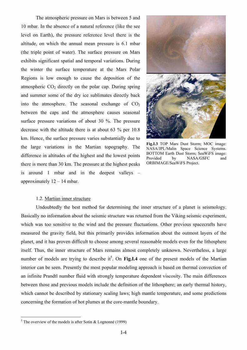
Dust and water ice particles can also strongly affect the atmospheric absorption and scattering
of the visible and thermal radiation and thus to modify the atmospheric circulation. These effects are
most common around the large volcanoes, the winter polar cap and globally, during dust storms
(Fig.I.3). Although, the atmosphere always contains enough aerosols (dust and ice particles) to scatter
~ 40 % of the incoming solar radiation. The net atmospheric effects depend on the physical properties
(such as size and optical properties) and on the spatial and temporal distributions of the aerosols. The
aerosols cause a strong decrease of the surface and near-surface daily temperatures as well as a
reduction in the vertical rate of change in temperature2.
The Martian near-surface atmospheric temperatures have been measured at the three landing
sites in the northern hemisphere: predominantly at the two Viking Lander sites3 for one or more
Martian years and by Pathfinder4 for about 1/8 Martian year during the summer. Elsewhere the surface
temperatures have been measured from orbit. The lowest surface temperatures occur in the southern
polar region during the winter. There they can go down to 148 K. The highest observed surface
temperature have been measured in the summer in northern mid-latitudes and goes up to 293 – 298 K.
In the Polar Regions the annual mean-surface temperature is between 158 and 163 K and at the
equator, between 218 and 223 K. The typical diurnal temperature variations as measured by the
Viking Landers at 1.5 m height above the surface showed values of around 70 K (Tillman et al. 1979).
The Mars Pathfinder performed these measurements at three heights (0.25, 0.5, 1 m) and found the
temperature to change very rapidly with height. The reason for that is the thin atmosphere. But during
dust storms the difference of 70 K can be reduced to 6 K or even less. One very useful link is:
http://www-mars.lmd.jussieu.fr/mars/live_access.html. It gives the opportunity to make a coarse
forecast of the weather on Mars as well as the thickness if the dry ice coverage at different places,
using the Martian Global Circulation Model linked to the Mars Climate Database.
2 A serious book, dealing with the Martian atmosphere, far not suitable for everybody is the one of Read & Lewis (2004). It can be described with four words “dynamic meteorology of Mars” 3 VL1 landed at Chryse Planitia (22.48° N, 49.97° W planetographic, 1.5 km below the datum and 6.1 mbar elevation). VL2 landed at Utopia Planitia (47.97° N, 225.74° W, 3 km below the datum elevation) 4 Mars Pathfinder landed at 19.3oN and 33.6oW.
I-3
The atmospheric pressure on Mars is between 5 and
10 mbar. In the absence of a natural reference (like the see
level on Earth), the pressure reference level there is the
altitude, on which the annual mean pressure is 6.1 mbar
(the triple point of water). The surface pressure on Mars
exhibits significant spatial and temporal variations. During
the winter the surface temperature at the Mars Polar
Regions is low enough to cause the deposition of the
atmospheric CO2 directly on the polar cap. During spring
and summer some of the dry ice sublimates directly back
into the atmosphere. The seasonal exchange of CO2
between the caps and the atmosphere causes seasonal
surface pressure variations of about 30 %. The pressure
decrease with the altitude there is at about 63 % per 10.8
km. Hence, the surface pressure varies substantially due to
the large variations in the Martian topography. The
difference in altitudes of the highest and the lowest points
there is more than 30 km. The pressure at the highest peaks
is around 1 mbar and in the deepest valleys –
approximately 12 – 14 mbar.
Fig.I.3 TOP Mars Dust Storm; MOC image: NASA/JPL/Malin Space Science Systems.BOTTOM Earth Dust Storm; SeaWiFS image: Provided by NASA/GSFC and ORBIMAGE/SeaWiFS Project.
1.2. Martian inner structure
Undoubtedly the best method for determining the inner structure of a planet is seismology.
Basically no information about the seismic structure was returned from the Viking seismic experiment,
which was too sensitive to the wind and the pressure fluctuations. Other previous spacecrafts have
measured the gravity field, but this primarily provides information about the outmost layers of the
planet, and it has proven difficult to choose among several reasonable models even for the lithosphere
itself. Thus, the inner structure of Mars remains almost completely unknown. Nevertheless, a large
number of models are trying to describe it5. On Fig.I.4 one of the present models of the Martian
interior can be seen. Presently the most popular modeling approach is based on thermal convection of
an infinite Prandtl number fluid with strongly temperature dependent viscosity. The main differences
between those and previous models include the definition of the lithosphere; an early thermal history,
which cannot be described by stationary scaling laws; high mantle temperature, and some predictions
concerning the formation of hot plumes at the core-mantle boundary.
5 The overview of the models is after Sotin & Lognonné (1999)
The oxygen atoms of the water molecules in ice Ih are arranged in layers of hexagonal rings.
The atoms of each hexagonal ring are displaced with respect to each other alternately in two planes.
The resulting hexagonal channels make ice Ih an open structure (see Fig.I.6). Its space group is
P63/mmc. In reality the water molecules experience small displacements from the shown positions.
Therefore, the arrangement on Fig.I.6 should be regarded as an averaged over space and time
formation. More details about the hexagonal ice structure and its properties can be found in Kuhs &
Lehmann (1986), Petrenko & Whitworth (1999). The water molecules on the ice surface are poorly
bound because they interact with other molecules only from one side. It makes the structure of the free
I-6
surface to some extent different from the one of the bulk. A number of experimental and theoretical
studies on the structure and the physical properties of the ice surface (e.g. Petrenko and Whitworth
1999) showed the importance and complexity of such investigations, especially close to the ice
melting point. Dash (1995) and Wettlaufer (1997) discussed theoretically the phenomenon of surface
premelting or the existence of a quasi-liquid layer at temperatures and pressures below the melting
point. Bluhm et al. (2002) presented experimental observations on the premelting of ice showing the
existence of a quasi-liquid layer at temperatures between -20°C and 0°C. When the temperature
approached the ice melting point the film was about 30 Å thick and at 253K it became insignificant.
Fig.I.6 Structure of ice Ih (taken from Lobban 1998). The right and the left pictures show the structure as seen parallel and perpendicular to the hexagonal channels, respectively.
2.2. Hydrate structures and phase diagram
Clathrate hydrates comprise a class of ice-like solids in which, usually apolar guest molecules
occupy, fully or partially, cages in the host structure formed by H-bonded water molecules. Different
people give different names to this structure – gas clathrates, gas hydrates, clathrates, hydrates etc –
but they all mean the same. They exist as stable compounds at high pressure and/or low temperature
(van der Waals and Platteeuw, 1959).
The gas hydrates (hence this will be the name most frequently used in this work) usually form
two crystallographic cubic structures – structure (Type) I and structure (Type) II (von Stackelberg &
Müller, 1954) of space groups nPm3 and mFd 3 respectively. Rather seldom a third hexagonal
structure of space group P6/mmm maybe observed (Type H).
The unit cell of Type I consists of 46 water molecules, forming two types of cages – small and
large (see Fig.I.7). The small cages in the unit cell are two against six large ones. The small cage has
the shape of pentagonal dodecahedron (512) (see Fig.I.7) and the large one that of tetrakaidecahedron
(51262). Typical guests forming Type I hydrates are CO2 and CH4.
The unit cell of Type II consists of 136 water molecules, forming also two types of cages –
small and large. In this case the small cages in the unit cell are sixteen against eight large ones. The
I-7
small cage has again the shape of pentagonal dodecahedron (512) but the large one this time is
hexakaidecahedron (51264). Type II hydrates are formed by gases like O2 and N2.
The unit cell of Type H consists of 34 water molecules, forming three types of cages – two
small of different type and one huge. In this
case, the unit cell consists of three small cages
of type 512, twelve small ones of type 435663
and one huge of type 51268. The formation of
Type H requires the cooperation of two guest
gases (large and small) to be stable. It is the
large cavity that allows structure H hydrates
to fit in large molecules (e.g. butane,
hydrocarbons), given the presence of other
smaller help gases to fill and support the
remaining cavities. Structure H hydrates were
suggested to exist in the Gulf of Mexico.
There thermogenically-produced supplies of
heavy hydrocarbons are common.
Fig.I.7 Schematic of the cages, building the unit cells of the different hydrate structures
The importance of the
gas hydrates here on Earth is out
of any doubt. The kinetics of
their formation and
decomposition, as well as their
physical properties are of a
significant importance for the
gas industry, economy and
ecology. Anyway, the topic of
this work is the gas hydrates on
Mars; therefore I am not going to
enter into a detailed discussion
about their role on our planet.
But their importance in cosmic
scale and especially for Mars
will be debated in the next
paragraph.
Fig.I.8 CO2 hydrate phase diagram. The black squares show experimental data (after Sloan, 1998). The lines drawing CO2 phase boundaries are calculated according to the Intern. thermodyn. tables (1976). The water phase boundaries are only guides to the eye.
The hydrate structures are stable at different pressure-temperature conditions depending on the
guest molecule. Here one Mars related phase diagram of the CO2 hydrate combined with those of pure
I-8
CO2 and water is given (Fig.I.8). The CO2 hydrate has two quadruple points: (I-Lw-H-V) (T = 273.1
K; p = 12.56 bar) and (Lw-H-V-LHC) (T = 283.0 K; p = 44.99 bar) (Sloan, 1998). The CO2 itself has a
triple point at T = 216.58 K and p = 5.185 bar and a critical point at T = 304.2 K and p = 73.858 bar.
The dark gray region (V-I-H) represents the conditions at which the CO2 hydrate is stable together
with gaseous CO2 and water ice (below 273.15 K). On the horizontal axes the temperature is given in
Kelvin and Celsius (down and up respectively). On the vertical ones the pressure (left) and the depth
in the Martian regolith (right) are given. The horizontal dashed line at zero depth represents the
average surface conditions. The two bent dashed lines show two calculated Martian geotherms after
Stewart & Nimmo (2002) at 30o and 70o latitude. I will come back to this phase diagram several times
later on.
As a matter of fact, probably the first evidence for the existence of CO2 hydrates dates back to
the year 1882, when Wroblewski (1882a, b and c) reported clathrate formation while studying
carbonic acid. He noted that the gas hydrate was a white material resembling snow and could be
formed by raising the pressure above certain limit in his H2O – CO2 system. He was the first to
estimate the CO2 hydrate composition, finding it to be approximately CO2·8H2O. He also mentions
that “…the hydrate is only formed either on the walls of the tube, where the water layer is extremely
thin or on the free water surface…” This already indicates the importance of the surface available for
reaction, i.e. the larger the surface the better. Later on in 1894, Villard deduced the hydrate
composition as CO2·6H2O. Three years later, he published the hydrate dissociation curve in the range
267 K – 283 K (Villard 1897). Tamman & Krige (1925) measured the hydrate decomposition curve
from 253 K down to 230 K and Frost & Deaton (1946) determined the dissociation pressure between
273 and 283 K. Takenouchi & Kennedy (1965) measured the decomposition curve from 45 bars up to
2 kbar. For the first time the CO2 hydrate was classified as a Type I clathrate by von Stackelberg &
Muller (1954).
2.3. Formation and decomposition kinetics
Since the 1950s, a large number of gas hydrate systems have been studied but still many of
their physico-chemical properties as well as their formation and decomposition kinetics are not well
understood, despite their importance for a number of reasons (e.g. Sloan 1998).
A review of the kinetics of gas hydrate formation in aqueous laboratory systems can be found
in Sloan (1998). The nucleation and the induction period of the gas hydrate formation in aqueous
solutions are described within the frames of the General Nucleation Theory in the papers of Kashchiev
and Firoozabadi (2002, 2003). Also a hypothetical microscopic mechanism for the nucleation of
hydrate from ice with an emphasize put on the role of the quasi-liquid layer can be found in Sloan and
Fleyfel (1991). Schmitt (1986) performed experimental measurements of the induction period of the
CO2 hydrate formation at low temperatures. No clear dependence on the temperature and the
I-9
overpressure was observed. A strong dependence of the transformation rates on the surface area of the
gas-ice contact was demonstrated by Barrer and Edge (1967). Later, Hwang et al. (1990) studied the
methane-hydrate growth on ice as a heterogeneous interfacial phenomenon and measured the clathrate
formation rates during ice melting at different gas pressures. Sloan and Fleyfel (1991) discussed
molecular mechanisms of the hydrate-crystal nucleation on ice surface, emphasizing the role of the
quasi-liquid-layer (QLL). Takeya et al. (2000) made in-situ observations of the CO2-hydrate growth
from ice-powder for various thermodynamic conditions using laboratory X-ray diffraction. They
distinguished the initial ice-surface coverage stage and a subsequent stage, which was assumed to be
controlled by gas and water diffusion through the hydrate shells surrounding the ice grains. The
process was modeled following Hondoh and Uchida (1992) and Salamatin et al. (1998) in a single ice
particle approximation. The respective activation energies of the ice-to-hydrate conversion were
estimated to be 19.2 and 38.3 kJ/mol. The first in-situ neutron diffraction experiments on kinetics of
the clathrate formation from ice-powders were presented by Henning et al. (2000). They studied the
CO2-hydrate growth on D2O ice Ih, using the high intensity powder diffractometer HIPD at Argonne
National Laboratory for temperatures from 230 to 263 K at a gas pressure of approximately 6.2 MPa.
The starting material was crushed and sieved ice with unknown but most likely irregular shape of the
grains. To interpret their results at a later stage of the hydrate formation process, the authors applied a
simplified diffusion model of the flat hydrate-layer growth, developed for the hydration of concrete
grains (Berliner et al. 1998; Fujii and Kondo 1974), and determined the activation energy of
27.1 kJ/mol. This work has been continued by Wang et al. (2002) to study the kinetics of CH4-hydrate
formation on deuterated ice particles. A more sophisticated shrinking-ice-core model (Froment and
Bischoff 1990; Levenspiel 1999) actually reduced to the diffusion model of Takeya et al. (2000; 2001)
has been used to fit the measurements. Higher activation energy of 61.3 kJ/mol was deduced for the
methane hydrate growth on ice. Based on Mizuno and Hanafusa (1987), the authors suggested that the
quasi-liquid layer of water molecules at the ice-hydrate interface may play a key role in the (diffusive)
gas and water redistribution although a definite proof could not be given.
One of the recent and most intriguing findings is that, at least in cases where the guest species
are available as excess free gas, some gas hydrate crystals grow with a nanometric porous
microstructure. Using cryo field-emission scanning electron microscopy (FE-SEM), direct
observations of such sub-micron porous gas hydrates have now repeatedly been made (Klapproth
2002; Klapproth et al. 2003; Kuhs et al. 2000; Staykova et al. 2002; Staykova et al. 2003; Genov et al.
2004). Hwang et al. (1990) reported that the methane hydrates formed from ice in their experiments
were bulky and contained many voids. Rather interestingly, there is evidence that besides dense
hydrates, some natural gas hydrates from the ocean sea floor also exhibit nanometric porosity (Suess et
al. 2002). Based on experimental studies (Aya et al. 1992; Sugaya and Mori 1996; Uchida and
Kawabata 1995) of CO2 and fluorocarbon hydrate growth at liquid-liquid interfaces, Mori and
I-10
Mochizuki (1997) and Mori (1998) had already proposed a porous microstructure of the hydrate layers
intervening the two liquid phases and suggested a phenomenological capillary permeation model of
water transport across the films. Although general physical concepts of this phenomenon in different
situations may be quite similar, still there are no sufficient data to develop a unified theoretical
approach to its modeling (Mori 1998).
In accordance with numerous experimental observations (Henning et al. 2000; Kuhs et al.
2000; Staykova et al. 2002; 2003; Stern et al. 1998; Takeya et al. 2000; Uchida et al. 1992; 1994), a
thin gas hydrate film rapidly spreads over the ice surface at the initial stage of the ice-to-hydrate
conversion (stage I after Staykova et al. 2002, 2003). Subsequently, the only possibility to maintain
the clathration reaction is the transport of gas molecules through the intervening hydrate layer to the
ice-hydrate interface and/or of water molecules from the ice core to the outer hydrate-gas interface. As
mentioned above, a diffusion-limited clathrate growth was assumed for this second stage described by
Takeya et al. (2000), Henning et al. (2000), and Wang et al. (2002) on the basis of the shrinking-core
models formulated for a single ice particle, in their treatment without taking explicitly account of a
surface coverage stage. Salamatin and Kuhs (2002) suggested in the case of porous gas hydrates, the
gas and water mass transport through the hydrate layer becomes much easier, and the clathration
reaction itself together with the gas and water transfer over the phase boundaries may be the rate-
limiting step(s) of the hydrate formation that follows the initial coverage and this process should be
modeled simultaneously with the ice-grain coating (stage II after Staykova et al. 2002, 2003). Still
they expect an onset of a diffusion-limited stage (stage III in this nomenclature) of the hydrate
formation process completely or, at least, partly controlled by the gas and water diffusion through the
hydrate phase. The values for the activation energies for the CH4 hydrate formation case they obtained
were 39.9 kJ/mol (with D2O ice) and 34 kJ/mol (with H2O ice) for the reaction-limited stage and 59.9
kJ/mol for the diffusion limited one. Later on, to improve the fit of the initial part of the reaction, the
first stage was divided into two sub stages (Genov et al. 2004) – stage Ia and stage Ib. Stage Ib was the
previously mentioned surface coverage, preceded by a crack filling stage Ia. In the case of CO2,
hydrate they reported activation energies for stage I 5.5 kJ/mol at low temperatures and 31.5 kJ/mol
above 220 K; 42.3 kJ/mol for stage II and 54.6 kJ/mol for stage III.
The anomalous preservation is a well established but little-understood phenomenon of a long-
term stability of gas hydrates outside their stability field. It occurs after some initial hydrate
decomposition into ice in certain temperature range. It is a very interesting phenomenon of substantial
scientific and practical interest. Davidson et al (1986) performed early observations of this effect. Such
were made independently in more detailed, by Yakushev & Istomin (1992). These authors observed an
unexpected perseverance when gas hydrates were brought outside their stability field at temperatures
below the ice melting point. More recently, Stern et al. (2001) and Takeya et al. (2001) investigated
the temperature dependency of the effect in the methane hydrate case and found that the effect also
I-11
had a lower limit. According to Stern et
al. (2001) the “anomalous preservation
window” is between 240K and the ice
melting point, while at temperatures
below 240K the decomposition is rapid
and appears to be thermally activated.
Within this window the decomposition
rates vary considerably by several
orders of magnitude in a reproducible
way (see Fig.I.9) with two minima at
around 250 and 268 K. Takeya et al.
2002 confirmed this effect and
suggested diffusion limitation for explaining the slow decomposition kinetics within the anomalous
preservation window. A similar, but not identical behaviour was observed for CO2 hydrate (Stern et al.
2003). Still, the deeper physical origin of “anomalous preservation” remains obscure and the
controlling parameters elusive (Wilder & Smith 2002, Stern et al. 2002, Circone et al. 2004). This
effect may lead to a revision of the existing ideas about the importance of the CO2 decomposition for
the processes running on Mars (see § 3).
Fig.I.9 Self-preservation of CH4. (Stern et al. 2001)
§ 3. CO2 hydrates on Mars
Iro et al. (2003), trying to interpret the nitrogen deficiency in comets, discussed in detail the
conditions needed to form clathrate hydrates in the proto-planetary nebulae, surrounding the pre-main
and main sequence (MS) stars. They stated most of the conditions for hydrate formation were fulfilled,
despite the rapid grain growth to meter scale. The key was to provide enough microscopic ice particles
exposed to a gaseous environment. De facto, observations of the radiometric continuum of
sircumstellar discs around τ-Tauri and Herbig Ae/Be stars suggest massive dust disks consisting of
millimeter-sized grains, which disappear after several millions of years (e.g. Beckwith et al. 2000,
Natta et al. 2000). A lot of work on detecting water ices in the Universe was done on the Infrared
Space Observatory (ISO). For instance, broad emission bands of water ice at 43 and 60 µm were found
in the disk of the isolated Herbig Ae/Be star HD 100546 in the constellation Musca. The one at 43 µm
is much weaker then the one at 60 µm, which means the water ice, is located in the outer parts of the
disk at temperatures below 50 K (Malfait et al. 1998). There is also another broad ice feature between
87 and 90 µm, which is very similar to the one in NGC 63026 (Barlow 1997). Crystalline ices were
also detected in the proto-planetary disks of ε-Eridani and the isolated Fe star HD 142527 (Li, Lunine
6 The Butterfly nebula in Scorpius.
I-12
& Bendo 2003, Malfait et al. 1999) in Lupus. 90 % of the ice in the latter was found crystalline at
temperature around 50 K. HST demonstrated that relatively old circumstellar disks as the one around
the 5 million year old B9.5Ve (Jaschek & Jaschek 1992) Herbig Ae/Be star HD 141569A are dusty
(Fig.I.10) (Clampin et al. 2003). Li & Lunine (2003) found water ice there. Knowing the ices usually
exist at the outer parts of the proto-planetary nebulae, Hersant et al. (2004) proposed an interpretation
of the volatile enrichment, observed in the four giant planets of the Solar System, with respect to the
Solar abundances. They assumed the volatiles had been trapped in the form of hydrates and
incorporated in the planetesimals flying in the proto-planets’ feeding zones. Obviously, the idea that
the gas hydrates may play a role in a cosmic scale starts to gain in popularity. Nevertheless, the
pressure and temperature conditions in the outer space and on Mars are distinctly different.
There is a well-known meteorological phenomenon called diamond dust production. At
temperatures below –18 oC, ice Ih crystals may form as irregular hexagonal plates or non-branched ice
needles or columns directly from water vapor in the air, through a process called deposition. Their size
may go below 20 µm across, which may result in “snow” with a very high specific surface area. The
ice existing and forming on Mars is most likely ice Ih in the shape of diamond dust.
CO2 is an abundant volatile on Mars. It dominates
in the atmosphere and covers the polar ice caps much of
the time. In the early seventies, the possible existence of
CO2 hydrates on Mars was proposed (Miller & Smythe
1970). Recent consideration of the temperature and
pressure of the regolith and of the thermally insulating
properties of dry ice and CO2 clathrate (Ross and Kargel,
1998) suggested that dry ice, CO2 clathrate, liquid CO2,
and carbonated groundwater are common phases even at
Martian temperatures (Lambert and Chamberlain 1978,
Hoffman 2000, Kargel et al. 2000).
What if CO2 hydrates are present in the Martian
polar caps as some authors suggest (e.g. Clifford et al. 2000, Nye et al. 2000)? Clifford (1980a, 1980b,
1993) first proposed that Chasma Boreale and Chasma Australe were possibly formed by a
jökulhlaup-type event. He noted the large size of these reentrants and the fact that they crosscut typical
polar channels and are geomorphologically similar to Ravi Vallis – an outflow channel with a flood
origin (Fig.I.11). Clifford (1980b) hypothesized a basal melting in the past history of the polar cap
was possible and that melt water could collect within and be catastrophically released from craters
beneath the cap, resulting in a jökulhlaup. Heat generated by turbulence and viscous dissipation within
the flowing water and by friction between the flowing water and surrounding ice could then serve to
enlarge the drainage tunnel.
Fig.I.10 Coronographic image of HD 141569
I-13
But if the polar caps contain
significant amounts of CO2 hydrate mixed
with water ice (Jakosky et al. 1995, Hoffman
2000), then the cap will not melt as readily as
it would if consisting only of water ice,
because of the clathrate’s lower thermal
conductivity, higher stability under pressures
and higher strength (Durham 1998), compared
to the pure water ice. Thus, obtaining an
accurate estimate of the amount of CO2
clathrate in the layered deposits is of major
importance. Mellon (1996) studied this
problem and found that the polar deposits probably contain relatively small amounts of CO2.
However, if the polar deposits contain significant amounts of CO2 clathrate, this would affect the
behavior of the melted polar material. Under constant pressure but increasing temperature beneath the
cap, the decomposed CO2 clathrate would release liquid CO2 (soluble in water at low temperatures and
high pressures), liquid water
and excess, gaseous CO2
(Hoffman 2000). When this
melt mixture reaches the cap
periphery, and pressure is
therefore greatly reduced, the
water would readily freeze
and CO2 would now be
nearly completely insoluble,
leaving unstable pockets of
CO2 gas within the ice which would be likely to burst (Hoffman 2000).
Fig.I.11 Formation of Chasma Boreale by an outflow of melt water (from Fishbaugh & Head 2002).
Fig. I.12 The Martian South Polar Cap as seen in terms of H2O (left), CO2 (middle) and normally (right). The arrows show the suspected clathrate containing regions. Courtesy: Mars Express, OMEGA team. Image Number: SEMVMA474OD
The question of a possible diurnal and annual CO2 hydrate cycle on Mars also stays, since the
large temperature amplitudes observed there cause leaving and reentering the clathrate stability field
on daily and seasonal basis. The question is can the gas hydrate be detected by any means, being
deposited on the surface. Probably yes. The OMEGA spectrometer on board of Mars Express returned
some data, which were used by the OMEGA team to produce images of the south polar cap, as it was
visible in terms of CO2 and H2O (Fig.I.12). The arrows assign areas where the existence of dry ice is
not very likely but still it is visible and a strong water ice signal can be detected. If one looks back at
the phase diagram from Fig.I.8 will see that dark gray p-T region where the water ice coexists with
gaseous CO2 and CO2 hydrate. It is not clear if this is hydrate, because the images are in a rainbow
I-14
scale, which is not published yet and will not be available before the beginning of the year 2005 due to
technical problems (OMEGA team private communication April 2004). Otherwise, one approach to
see if this is hydrate or not is to try to find there the “golden ratio” of ≈ 6:1 water to CO2 molecules. In
any case this is still an open question.
The decomposition of CO2 hydrate is believed to play a significant role in the terra-forming
processes on Mars. Many of the observed surface features are partly attributed to it. For instance,
Musselwhite et al. (2001) argued that the Martian gullies (Fig.I.13) had been formed not by liquid
water but by liquid CO2 since the present Martian climate does not allow liquid water existence at the
surface in general. Especially this is true for the southern hemisphere where most of the gully
structures occur. However, water can be present there as ice Ih, CO2 hydrates or hydrates of other
gases (e.g. Max & Clifford 2001, Pellenbarg et al. 2003) or liquid water at depths below 2 km under
the surface (see geotherms in the phase diagram Fig.I.8). With the present obliquity, the slopes where
the gullies occur remain generally shaded during most of the year and are among the coldest spots on
the planet. At such conditions, any dry ice just below the surface and in diffusive contact with the
surface should remain stable and act as a dam trapping gas hydrate, water ice and liquid CO2
underneath. In case of temperature increase the dry ice dam will get molten and the liquid CO2 will
drain out. It will rapidly vaporize. Some of the vapor may snow out, but the rapid expansion should be
enough to create a fluidized suspended flow of CO2 gas along with some entrained debris. The
clathrate hydrate will dissociate into CO2 vapor plus water ice and the additional gas release should
help to maintain the flow. Gully formation by this process can be in single or multiple episodes
depending on the rate of replenishment of the liquid-CO2 aquifer and the formation of a new dry-ice
plug. It is believed that the melting of ground-ice by high heat flux has formed the Martian chaotic
terrains (Mckenzie & Nimmo 1999). Milton (1974)
suggested the decomposition of CO2 clathrate had
caused rapid water outflows and formation of
chaotic terrains. When sediment saturated with
water becomes subjected to a stress, a loosely
packed grain framework suddenly collapses and the
grains become temporarily suspended in the pore
fluid (liquefaction) (see Fig.I.14). If water flows
fast enough so that it balances with the settling
velocity of grains, the grains are suspended in the
stream and the water-sediment mixture behaves like
fluid (fluidization). These two processes may have
played important roles in the chaotic terrain formation (Ori & Mosangini 1997). If the amount of gas
derived from clathrate is large enough and conditions for gas build-up under an impermeable layer
Fig.I.13 Gullies on a Crater Wall in Newton Basin MGS MOC Release No. MOC2-317, 8 August 2002
I-15
exist, the pressure release of gas can play a major role in pulverizing rocks and remaining ices.
Furthermore fragmented rocks by gas explosion can liquefy easily. Once liquefied and fluidized the
mobilized water-sediment mixture flows out catastrophically. In some cases, ponds of water may have
occurred in the depressions inside the chaotic terrain (Ori & Mosangini 1998). Ness & Orme (2002)
gave a similar explanation of the formation of the Martian spiders. In their interpretation the process
did not reach the stage of catastrophic flooding but stopped after intensive out-gassing and several
other events linked in one or another way with the CO2 hydrate formation and decomposition.
Cabrol et al. (1998) proposed that the physical environment and the morphology of the south
polar domes on Mars suggest for possible cryovolcanism. The surveyed region consisted of 1.5-km
thick-layered deposits covered seasonally by CO2 frost (Thomas et al. 1992) underlain by H2O ice and
CO2 hydrate at depths > 10m (Miller and Smythe, 1970). When the pressure and the temperature are
raised above the stability limit, the clathrate is decomposed into ice and gases, resulting in explosive
eruptions. Cabrol et al. observed these pancake-shaped domes only in impact structures and suggested
morphogenic processes associated with high pressure and high temperature conditions, created by
meteorite impacts that can generate eruptive conditions for clathrates. All the domes are observed at
the bottom of impact craters, and range between 40 - 50-km in diameter, with a few larger or smaller
exceptions. They are round at their base and show concentric rings. This observation rules out the
possibility of an aeolian construct. Their comparison illustrates a process of dome formation most
likely by the emergence of underground material, which can be compared to the formation of
terrestrial volcanic lava domes.
Fig.I.14 Chaotic terrain (left: Courtesy ESA Mars Express 2004) and a possible mechanism of its formation (right: after Komatsu et al. (2000)).
Still a lot more examples of the possible importance of the CO2 hydrate on Mars can be given.
One thing remains unclear: is it really possible to form hydrate there? Kieffer (2000) suggests no
I-16
I-17
significant amount of clathrates could exist near the surface of Mars. Stewart & Nimmo (2002) find it
is extremely unlikely that CO2 clathrate is present in the Martian regolith in quantities that would
affect surface modification processes. They argue that long term storage of CO2 hydrate in the crust,
hypothetically formed in an ancient warmer climate, is limited by the removal rates in the present
climate. Other authors (e.g. Baker et al. 1991) suggest that, if not today, at least in the early Martian
geologic history the clathrates may have played an important role for the climate changes there. Since
not too much is known about the CO2 hydrates formation and decomposition kinetics, their physical
and structural properties, it becomes clear that all the above mentioned speculations rest on extremely
unstable basis. How fast do CO2 hydrates form? What limits their growth? What controls the hydrate
decomposition? Is a catastrophic decomposition likely? Are the physics behind the hydrate formation
and decomposition similar? Can we describe better the hydrate microstructure, which certainly affects
its physical and mechanical properties? This work comes to try to throw more light upon these issues.
Chapter II
Methods and instrumentation
In this chapter will be discussed the basic physics of the neutrons, such as their physical
properties and interactions in which they play a role. A special emphasize will be put on the neutron
scattering, neutron production and detection. Some other processes involving neutrons, which do not
have a direct impact on the present studies will be mentioned very briefly. Also will be given a
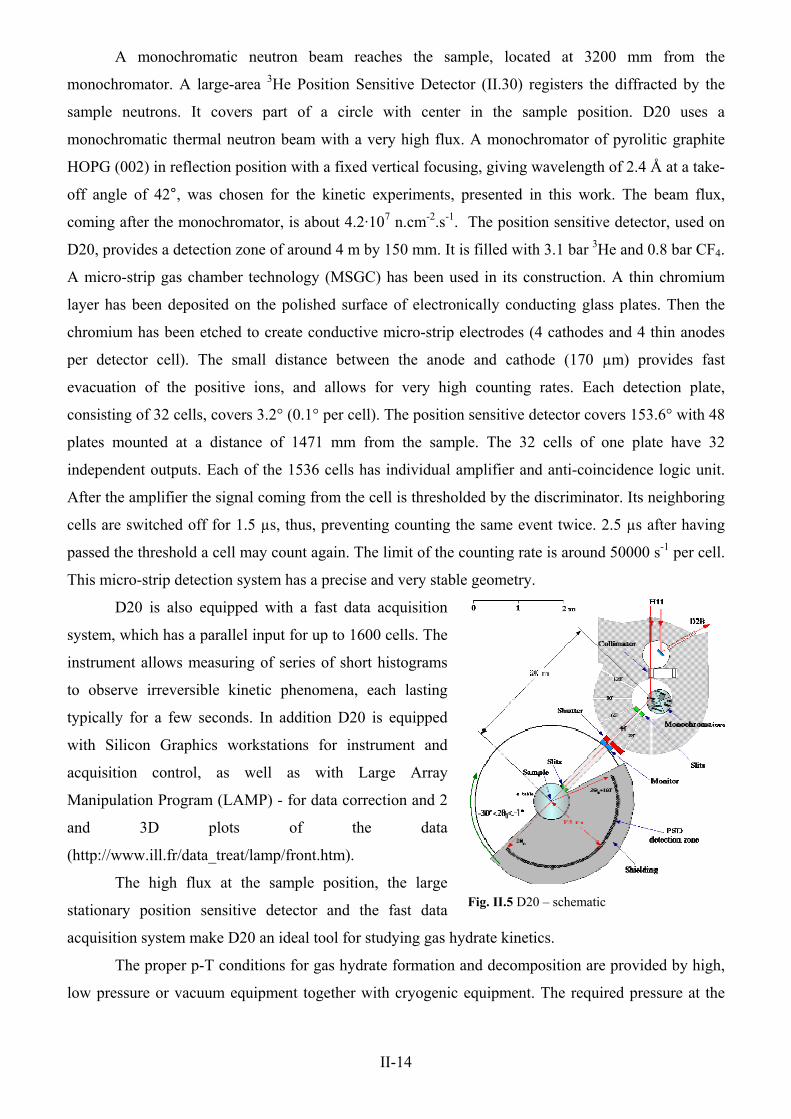
description of the instrument used in these studies – D20 – and certain issues of the radiation
protection will be conversed. Later on the pVT system used in the in-house work will be described and
its main ideology discussed. Then, the main principles of the electron microscopy will be introduced,
together with some basic information on the physics of the electrons and a description of LEO 1530
Gemini – the cryo FE-SEM used here. At the end of the chapter, the BET method for measuring
specific surface area will be briefly described.
§ 1. Neutrons – basic physics and instruments
1.1. Neutrons – basic physical properties
In the year 1930 Bothe and Becker performed an experiment on bombardment of beryllium
with alpha particles. They detected highly penetrating radiation, which they identified as γ-rays.
Frederic and Irene Joliot-Curie realized the considered radiation ejects protons out of paraffin target
and obtained the velocity of the ejected protons ≈ 3.3 x 10⁷ m/s. This was explained as a Compton
scattering of γ-rays from protons.
In 1932 James Chadwick (a student of Rutherford) carried out a series of experiments to define
the real nature of the “beryllium” rays. He investigated them passing not only through paraffin but also
through some other especially N-containing materials. Thus, he obtained the velocity of the ejected
nitrogen nuclei (≈ 4.7 x 10⁶ m/s). He rejected the hypothesis of the electromagnetic nature of this
radiation and assumed it to consist of neutral particles with a steady state mass close to that of the
proton (Chadwick 1932) – the neutron. For this, in 1935 he obtained the Nobel Prize in physics.
Let us have a fast look at the main properties of the neutrons as well as the interactions they
take part in.
Mass: Estimation about the mass of these particles could be done on the basis of the
conservation laws assuming them to be non-relativistic (with an accuracy of 1 %).
II-1
xx
xx
VMmvmv
VMmvmv
+=
+=
0
2220
222 (II. 1)
m and Mx are the masses of the unknown particle and the recoil nucleus respectively, v0 and v – the
velocity of the particle before and after the collision, Vx – the velocity of the nucleus. By solving
system (II.1) Chadwick got:
s a result, the neutron mass mn
the atomic nucleus consists of
neutron
e:
02 v
MmmV
xx += (II.2)
A = 939.57 Mev or 1.15 mp was found.
In the same year Ivanenko and Heisenberg suggested that
s and protons.
Electric Charg In the elementary particle physics as an electric charge of a particle is
underst
between the
particle
ood a discrete whole quantum number, whose conservation limits the possible kinds of
transformations of the particle. All elementary particles carry an elementary charge, equal either to 0 e
or to ±1 e. As a unit electric charge is taken the charge of the electron (1 e = 1.6 x 10⁻⁹ C).
From the other site, the electric charge is a quantitative measure for the interaction
s and the electric fields. The new theories unifying the forces require the neutron to be exactly
neutral. In this sense its charge is less then 10-21 e.
Spin: In the quantum mechanics is shown that the square magnitude of the orbital angular
momentum has a quantized spectrum of eigenvalues:
22)1( h
r+= lll )1( += lll h
r (II. 3)
where l is the azimuthal quantum number and for given principal quantum number n gets values l = 0,
or
1, 2……n – 1. The spectrum of the possible values of the projection of lr
over a given direction z has
(2l +1) values: 0;.....)1(; hh −±± ll . In the quantum physics only the maxi um projection of lmr
equal to
lh is measured.
The expe riments have shown that the elementary particles have inner angular momentum,
which has a quantum nature and is not connected with their orbital motion. It is called spin.
Analogously to the former may be shown that the eigenvalues of the square of the operator of the spin
are: 22 )1( h
r+= sss or )1( += sss h
r
s +1) different values. The neutrons have a spin
(II. 4)
The projection of over a given direction z has (2
=
sr
quantum number s ½. Thus, they follow the statistics of Fermi – Dirac and obey the principle of
II-2
Pauli, which states that in a quantum system two particles of the same type cannot be in the same
condition at the same time.
Magnetic momentum: From the classical electrodynamics is known that a particle with charge
e and mass m, has also a magnetic momentum µ. In the quantum mechanics is shown that the
magnetic momentum, which is due to the orbital motion of the particle, is equal to:
)1(2
+= llme
l hµ (II. 5)
and the one due to the spin is:
)1(2
+= ssmegs hµ (II. 6)
where g is the gyro magnetic ratio.
According to the equation of Dirac, a particle with spin equal to ½ should have a magnetic
momentum - one magneton, if the particle is charged and 0 magneton if it has a zero charge. The
experiments have shown anomalously high biases from the calculated values for the protons and
neutrons:
µp = 2.792763 µ0
µn = -1.91315 µ0
where µ0 is the nuclear magneton and is equal to pme 2/0 h=µ . This showed those particles had much
more complicated structure, impossible to be explained with simple assumptions. According to the
quantum chromodynamics, the hadrons (including the neutrons) consist of quarks, which together with
the leptons are the building units of the whole material world. They are fermions (spin 1/2) and have
non-zero steady state mass. The quarks interact between themselves with strong interactions carried by
the gluons - neutral bosons (spin 1), with a zero steady state mass. According to the fragrance (their
main characteristic) there are six quarks: u, d, s, c, b, t. The neutron has a udd structure.
1.2.Neutron interactions
1.2.1. Strong (nuclear) interactions
There are three types of strong interactions for the neutrons:
1. Neutron – proton interactions.
2. Neutron – neutron interactions.
3. Neutron – nucleus interactions.
The reaction cross-sections for the neutron case significantly
depend on its energy. The classification of the neutrons according to
their energies is given in Table II.1.
The nuclear interaction is, however weak in an absolute scale,
and therefore the neutrons can penetrate the sample and investigate the bulk properties
Name Energy [eV] Cold 0 – 0.005
Slow Thermal 0.005 – 0.5 Resonant 0.5 - 103
Intermediate 103 – 105 Fast 105 – 5 x 10⁷ Super fast > 5 x 10⁷ Table II.1 Neutron energy classification
II-3
1.2.2. Weak interactions
On the first place it appears with its beta decay:
eepn ν~++→ − t1/2 = 10.2 min (II. 7)
The neutron takes part in many other weak interactions, which will not be considered here.
1.2.3. Electromagnetic interactions
The neutrons that have wavelengths of the order of or bigger then the atomic
dimensions (En < 10 eV) take part in the electromagnetic interactions of the magnetic momentum of
the neutron with those of the electron layers of the atoms. These interactions can be used in a large
number of investigations in the field of the solid-state physics. The neutron can interact with the
electric fields of the nuclei as well as (n, e-) scattering is possible.
1.2.4. Radiative capture ((n, γ) reactions)
This is one of the most common reactions of the neutrons with the matter. It follows the
scheme,
γ+→+ + XXn AZ
AZ
110 (II. 8)
The latter nucleus is usually β-active. This type of reactions is typical for the slow and intermediate
neutrons and is widely used for their detection. It is also the main responsible for the activation of the
experimental equipment.
1.2.5. (n, p) reactions
It is typical for the fast neutrons.
YpXn AZ
AZ 1
11
10 −+→+ (II. 9)
This is an exothermal reaction because mn > mp. It cannot take part at low energies because the ejected
proton needs energy to jump over the Coulomb barrier.
1.2.6. (n, α) reactions
This is a reaction of the type,
YHeXn AZ
AZ
32
42
10
−−+→+ (II. 10)
It is typical mainly for the fast neutrons but in many cases the coulomb barrier of the nuclei for α
particles is too low and the reaction can happen even with thermal neutrons. Thus, for registration of
thermal neutrons the reaction,
MeVLiHeBn 8.273
42
105
10 ++→+ (II. 11)
is used.
Reactions resulting in producing more then one nucleon are also possible but will not be
considered here.
1.2.7. Neutron scattering1 1 This overview is based on: Pynn (1990) and Squires (1997)
II-4
When neutrons are scattered by matter, the process can change the momentum and the
energy of the neutrons and the matter. The scattering is not necessarily elastic because the atoms in the
matter can move to some extent. Therefore, they can recoil during a collision with a projectile, or if
they are moving when the neutron arrives, they can pass on or absorb energy.
The total momentum and energy are conserved. When a neutron is scattered it looses energy ε.
Knowing that
vmk rrh = (II. 12)
it is easy to see that the amount of momentum given up by the neutron during its collision, or the
momentum transfer, is
)( kkQ ′−=rr
hr
h (II. 13)
where is the wave vector of the incident neutrons and kkr
′r
is that of the scattered neutrons. The
quantity kkQ ′−=rrr
is the scattering vector, and the vector relationship betweenQr
, , and kkr
′r
can be
displayed in the scattering triangle (Fig.II.1). This triangle also emphasizes that the magnitude and
direction of Qr
are determined by the magnitudes of the wave vectors for the incident and scattered
neutrons and the deflection (scattering) angle 2θ. For elastic scattering (Fig.II.1a) = k , so ε = 0 and
applying a bit of trigonometry to the scattering triangle leads to
kr
′r
λθπ /sin4=Q .
In the neutron-scattering experiments, are measured the intensity of the scattered neutrons (per
incident neutron) as a function of Q and ε. This scattered intensity ),( εQIr
is often referred to as the
neutron scattering law for the sample.
In a complete and elegant analysis, van Hove showed in 1954 that the scattering law could be
written exactly in terms of time-dependent correlations between the positions of pairs of atoms in the
sample. His result is that ),( εQIr
is proportional to the Fourier transform of a function giving the
probability to find two atoms at a certain distance apart. Lets have a more detailed look at this.
He used the observation of Fermi that the actual interaction between a neutron and a nucleus
may be replaced by an effective potential, much weaker than the actual interaction. This pseudo-
potential causes the same scattering as the actual interaction but it is weak enough to be used in Born’s
perturbation expansion. The Born approximation says the probability an incident plane wave with a
wave vector k scattered by a weak potential Vr
)(rr to become an outgoing plane wave with a wave
vector is: k ′r
23.
23.. )()( ∫∫ =′− rdrVerderVe rQirkirki rr rrrrrr
(II. 14)
II-5
where the integration is over the volume
of the scattering sample. Even though
individual nuclei scatter spherically, V )(rr
represents the potential due to the entire
sample, and the resulting disturbance for
the assembly of atoms is a plane wave.
The potential to be used in (II. 14)
is the Fermi’s pseudo-potential, which for
a single nucleus is given by b )( jj rr rr−δ ,
where bj is the scattering length of a
nucleus labeled j at position jrr and δ is
the delta function of Dirac that is zero
unless the position vector rr coincides
with jrr . Thus, for an assembly of nuclei, such as a crystal, the potential V )(rr is the superposition of
individual neutron-nuclei interactions:
Fig. II. 1 Scattering triangles of (a) elastic scattering (k’ = k) and (b) inelastic scattering with gain (k’ > k) and loss (k’ < k) of energy from the projectile.
∑ −=j
jj rrbrV )()( rrr δ (II. 15)
The summation is over all nuclear sites in the crystal.
Using (II. 14) and (II. 15) van Hove showed that the number of neutrons scattered per incident
neutron is (van Hove’s neutron-scattering law):
∑ ∫∞
∞−
−−′=
lj
titrQirQilj dteeebb
kk
hQI jl
,
)(.)0(.1),( εεrrrrr
(II. 16)
The summation is over pairs of nuclei j and l and the nucleus labeled j is at position )(trjr at time t,
while the nucleus labeled l is at position )0(lrr at time t = 0. The angular brackets denote averaging
over all starting times for observations of the system, which is equivalent to an average over all
possible thermodynamic states of the sample. Let us treat equation (II. 16) as if it described a classical
mechanics system in order to clarify its physical meaning. The sum over atomic sites in (II. 16) can
then be rewritten as:
[ ] [ ]( )∑ ∫∑∞
∞−
−−− −−=lj
rQijllj
lj
trrQilj dtetrrrbbebb jl
,
.
,
)()0(. )()0(rrrrr rrrδ (II. 17)
Lets suppose for a second that the scattering lengths of all the atoms in the sample are the same
(bj = bl = b). The scattering lengths in (II. 17) can be removed from the summation, and the right-hand
side becomes:
II-6
N is the number of atoms in the sample. The delta function in the definition of G ),( trr is zero except
when the position of an atom l at time zero and the position of atom j at time t are separated by the
vector rr . ),( trG r is equal to the probability an atom to be at the origin of a coordinate system at time
zero and an atom to be at position rr at time t, because the delta functions are summed over all
possible pairs of atoms. ),( trG r is generally referred to as the time dependent pair-correlation function
because it describes how the correlation between two particles develops with time. (II. 16) can be
written as:
∫∞
∞−
− rdetrGNb rQi 3.2 ),(rrr
[ ]( )∑ −−=lj
jl trrrN
trG,
)()0(1),( rrrr δ(II. 18)
∫∞
∞−
−−′= rdtdeetrG
kk
hNbQI tirQi 3.
2
),(),( εεrrrr
(II. 19)
Thus, ),( εQIr
is simply proportional to the Fourier transform of a function giving the probability to
find two atoms at a certain distance apart. By inverting (II. 19), information about the structure and
dynamics of condensed matter may be obtained.
Actually, Van Hove’s formalism can be modified to expose two types of scattering effects. The
first is coherent scattering. Here the neutron wave interacts with the whole sample as a unit, thus
scattered waves from different nuclei interfere with each other. This type of scattering depends on the
relative distances between the constituent atoms and consequently gives information about the
structure. Elastic coherent scattering tells about the equilibrium structure, while inelastic coherent
scattering provides information about the collective motions of the atoms. The second type is the
incoherent scattering. Here the neutron wave interacts independently with every nucleus in the sample
in order that the scattered waves from different nuclei do not interfere but the intensities from each
nucleus just add up. For instance, the incoherent scattering may, be a result of the interaction of a
neutron wave with the same atom but at different positions and times, thus providing information
about diffusion.
Even for a sample made of a single isotope, the scattering lengths emerging in (II. 16) will not
be equal. This is because the scattering length of a nucleus depends on its spin. There is no correlation
between the spin and the position of a nucleus. Therefore, the scattering lengths from (II. 16) can be
averaged over the nuclear spin states without affecting the thermodynamic average (in the angular
brackets). After introducing a nuclear spin averaging the sum in (II. 16) becomes:
( )∑ ∑ ∑ −+=lj lj j
jjjljllj AbbAbAbb, ,
222 )()( (II. 20)
II-7
Ajl replaces the integral from (II. 16). The first term in the right-hand side of (II. 20) represents the
coherent scattering, and the second one corresponds to the incoherent one. Consequently, one can
define the coherent and incoherent scattering lengths as:
The expression for the coherent scattering law is a sum over j and l and thus involves
correlations between the position of an atom j at time zero and this of an atom l at time t. Though j and
l may sporadically be the same atom, in general they are not because of the large number N of nuclei
in the sample. Therefore, one can say coherent scattering basically describes interference between
waves produced by the scattering of a single neutron from all nuclei in a sample.
The incoherent scattering involves correlations between the position of an atom j at time zero
and the position of the same atom at time t. Consequently, here the scattered waves from different
nuclei do not interfere. Most often, the incoherent scattering intensity is the same for all scattering
angles, adding intensity to the background.
The simplest type of coherent neutron scattering is diffraction. Assume the atoms are arranged
at fixed positions in a lattice and a neutron beam is shooting at it. Let also the value of the incident
wave vector, is the same for all neutrons, i.e. they fly in parallel and have equal velocities. Because
the atoms and their associated nuclei are fixed by default, there is no change in the neutron’s energy
during the scattering and the scattering is elastic. When a projectile neutron wave arrives at each atom,
the atom becomes a center of a scattered spherical wave and interference will take place. As the waves
originate from a regular array of sites, the individual disturbances will reinforce each other only in
particular directions. These directions are closely related to the symmetry and spacing of the scattering
sites and can be used to deduce the symmetry of the lattice and the distances between the atoms.
kr
Though, the diffraction is an elastic scattering process (ε = 0), the diffractometers integrate
over the scattered neutrons energies. Therefore, rather then setting ε = 0 in (II. 16), to calculate the
diffracted intensity one integrates the equation over ε. This makes sure the effect of the atomic
vibrations is taken into account in the diffraction cross-section. The integration gives another delta
function, suggesting that the pair correlation function G ),( trr has to be evaluated at t = 0. Thus the
result for a single isotope crystal is:
∑ −−=lj
rrQicoh
ljebQI,
).(2)(rrrr
(II. 22)
If the atoms in the sample were really stationary, the thermodynamic averaging brackets could
be removed from (II. 22) since rj and rl would be constant. But de facto, the atoms oscillate around
their equilibrium positions. When this is taken into account, the thermodynamic average introduces the
Debye-Waller factor, and (II. 16) becomes:
II-8
)(bbbinc −= 22
bbcoh = (II. 21)
221
,
).(2 )()(22
QSeebQIuQ
lj
rrQicoh
ljrr rrr
≡=−−∑ (II. 23)
where 2u is the average of the square of the displacement of an atom from its equilibrium position;
)(QSr
is the structure factor.
One can determine Qr
at which )(QSr
is nonzero and at which diffraction occurs. Presume Qr
is perpendicular to a plane of atoms and if it is any integer multiple of d/2π , (d is the distance
between parallel, neighboring planes of atoms) then Qr
(rj – rl) is a multiple of 2π and )(QSr≠ 0
because each exponential term in the sum in (II. 16) is unity. Thus, Qr
must be perpendicular to planes
of atoms in the lattice and must not satisfy the condition, S )(Qr
= 0, and there will be no scattering. If
one applies the condition described above
)/2( dnQ π= , n – integer (II. 24)
to the scattering triangle for elastic scattering and then uses the relationship between Q, θ and λ, will
obtain:
θλ sin2dn = (II. 25)
This equation, called Bragg’s law, relates the scattering angle 2θ, to the interplanar spacing in a
crystalline sample. Bragg’s law can also be understood in terms of the path-length difference between
waves scattered from neighboring planes of atoms (Fig.II.2). Diffraction (or Bragg scattering) may
occur for any set of atomic planes one can imagine in a crystal, providing the wavelength λ and the
angle θ between the projectile neutron beam and the planes satisfy (II. 25). Bragg scattering from a
particular set of atomic planes resembles
reflection from a mirror parallel to those
planes: the angle between the incident beam
and the plane of atoms equals the angle
between the scattered beam and the plane. If
a beam of neutrons of a particular wavelength
shoots on a single crystal, there will be no
diffraction. To obtain diffraction for a set of
planes the crystal must be rotated to the
correct orientation so that Bragg’s law is
satisfied.
Fig. II. 2. The extra distance passed by the wave reflected by the second scattering plane is 2d.sinθ. When this distance is set to be equal to nλ the result is again the Bragg’s law.
To this moment only a simple type of
crystal that can be built of unit cells, each
containing one atom was discussed. On the
II-9
other hand, polycrystalline powders, which consist of many randomly oriented single-crystal grains,
will diffract neutrons whatever the orientation of the sample relative to the incident beam of neutrons
is. There will always be grains in the powder that are correctly oriented to diffract. Thus, whenever the
scattering angle, 2θ, and the wavelength λ satisfy the Bragg equation for a set of planes, a reflection
independent of the sample orientation will be detected. This observation is the basis of the powder
diffraction.
1.3.Neutron production
1.3.1. Neutrons from nuclear fission (Balabanov 1998)
The process of decay of the excited nuclei into 2 (rarely 3 or 4) pieces with comparable
masses is called fission. O. Hahn, F. Strassmann, L. Meitner and O. Frisch discovered it in 1938 by
bombardment of uranium-235 with neutrons.
The energetic instability of the heavy nuclei follows from the relatively small mass defects and
the coulomb forces cause the fission. The fission of the heavy nuclei can be spontaneous or provoked
by collisions with neutrons, protons, γ-rays etc and brings some energy gain.
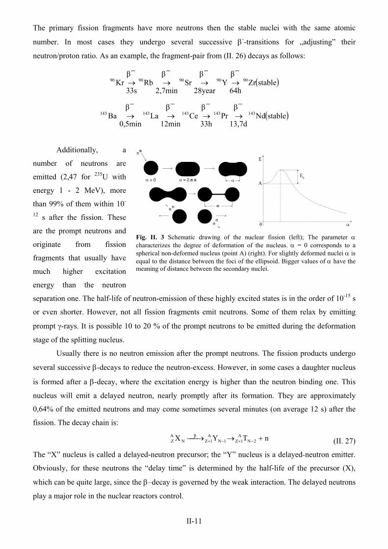
To split a nucleus a certain amount of energy is needed to deform it. If a spherical nucleus (α
= 0) is deformed to ellipsoidal its volume will not change because the nuclear matter is not deformable
but its surface will increase. From one side, this will cause an increase of the surface energy and the
nucleus will tend to recover its initial shape ∆Eattr. From the other side, this deformation will lead to
decreasing the coulomb repulsion energy ∆Erep. Obviously, if ∆Erep > ∆Eattr the nucleus will start to
increase its deformation and eventually split (Fig.II.3). The maximum of the curve on Fig.II.3b
corresponds to the state when the nucleus splits into two. The difference between the energy of the
non-excited state and the maximal one is the activation energy, Ea. It is equal to the kinetic energy of
the adsorbed neutron plus the binding energy fn of the neutron in the nucleus. If the binding energy is
bigger then the activation one the fission may take place even with thermal neutrons. This is the case
with 235U, where Ea = 5.8 MeV and fn = 6.4 MeV.
During the fission the 235U nucleus first absorbs a neutron, and a 236U compound nucleus is
formed in an excited state. It is unstable, and splits into two fragments2 (Keepin, 1969) (rarely more).
There are several hundred variants of splitting of 236U compound nucleus. Here is one of them:
235 236 90 143 3nU n U Kr Ba+ → → + +* (II. 26)
2 The nuclei formed within 10-14s are fission fragments. These fast nuclei slow down by colliding with the atoms of the fuel material, then pick-up electrons, and finally become neutral atoms. Since they are radioactive, they undergo several decay processes, and form the fission products.
II-10
The primary fission fragments have more neutrons then the stable nuclei with the same atomic
number. In most cases they undergo several successive β--transitions for „adjusting” their
neutron/proton ratio. As an example, the fragment-pair from (II. 26) decays as follows:
( )stableZrβ
64h Y
β
28year Sr
β
2,7min Rb
β
33s Kr 9090909090
−
→
−
→
−
→
−
→
( )stableNdβ
13,7d Pr
β
33h Ce
β
12min La
β
0,5min Ba 143143143143143
−
→
−
→
−
→
−
→
Additionally, a
number of neutrons are
emitted (2,47 for 235U with
energy 1 - 2 MeV), more
than 99% of them within 10-
12 s after the fission. These
are the prompt neutrons and
originate from fission
fragments that usually have
much higher excitation
energy than the neutron
separation one. The half-life of neutron-emission of these highly excited states is in the order of 10-15 s
or even shorter. However, not all fission fragments emit neutrons. Some of them relax by emitting
prompt γ-rays. It is possible 10 to 20 % of the prompt neutrons to be emitted during the deformation
stage of the splitting nucleus.
Fig. II. 3 Schematic drawing of the nuclear fission (left); The parameter α characterizes the degree of deformation of the nucleus. α = 0 corresponds to a spherical non-deformed nucleus (point A) (right). For slightly deformed nuclei α is equal to the distance between the foci of the ellipsoid. Bigger values of α have the meaning of distance between the secondary nuclei.
Usually there is no neutron emission after the prompt neutrons. The fission products undergo
several successive β-decays to reduce the neutron-excess. However, in some cases a daughter nucleus
is formed after a β-decay, where the excitation energy is higher than the neutron binding one. This
nucleus will emit a delayed neutron, nearly promptly after its formation. They are approximately
0,64% of the emitted neutrons and may come sometimes several minutes (on average 12 s) after the
fission. The decay chain is:
nTYX 2NA
1Z1NA
1Zβ
NAZ +→→ −+−+ (II. 27)
The “X” nucleus is called a delayed-neutron precursor; the “Y” nucleus is a delayed-neutron emitter.
Obviously, for these neutrons the “delay time” is determined by the half-life of the precursor (X),
which can be quite large, since the β–decay is governed by the weak interaction. The delayed neutrons
play a major role in the nuclear reactors control.
II-11
1.3.2. Neutron production via spallation
Another way of neutron production is to use an accelerator instead of a reactor. The
neutrons obtained that way are called spallation neutrons. This is done by letting high-energy protons
(or, less effectively, electrons) collide with a heavy-metal target, made of tungsten or uranium
(Fig.II.4). When a fast particle, such as the high-energy proton, bombards a heavy atomic nucleus,
some neutrons are “spalled”, or knocked out, in a nuclear reaction called spallation. Other neutrons are
“boiled off” as the bombarded nucleus heats up. It is something like when a bad Snooker player breaks
the balls at the start of the game using all the force he has. The result is that a few balls are
immediately ejected and many more will just start mooching around. For every proton striking the
nucleus, 20 to 30 neutrons are expelled. The accelerator coupled with a proton storage ring produces
the protons in bursts lasting for less than a microsecond. One of the advantages of a spallation source
is that only a small amount of energy (about 27 MeV per neutron) is deposited in the spallation target
by the protons. Nuclear fission produces at about four to five times more energy in generating each of
its neutrons. However, the price of producing the high-energy protons (electricity) is very high.
Neutrons from a spallation source arrive in pulses rather than continuously as they do at the
reactor. This means the monochromator crystal needed at
reactors, for instance, can be avoided and all the neutrons
can be used. The trick allowing for this is that one can
measure the time of flight of each detected neutron
between the moderator and the detector. From this time its
velocity and wavelength can be determined. Therefore,
generating a monochromatic beam is unnecessary.
A thermal neutron with energy of 25 MeV flies
with a speed of about 2.2 km/s (Mach 7). A typical neutron
spectrometer is about 10 m long, so the neutron travels
from the moderator to the detector in about 5 ms. Since the
duration of the neutron pulse emerging from the moderator
of a pulsed source is typically a few tens of microseconds, the time of flight of the neutron can be
determined with high relative precision.
Fig. II. 4 Mechanism of the neutron production via spallation
1.4.Neutron detection
The neutron detection is based on the registration of the products of the nuclear reactions they
cause. The neutron detector is an ordinary charged particle (or γ-quantum) detector whose working
media is rich in a solution reacting intensively with the neutrons. The large variety of nuclear reactions
caused by the neutrons and the different dependence of the reaction cross-sections on their energy
II-12
gives the opportunity different types of detectors to be constructed. All the methods for neutron
detection can be combined in several groups, briefly described below.
1.4.1. Radiative capture method
It is based on the registration of the γ-quanta coming from the radiative capture (n, γ)
reactions, charged particles or fission products. One very convenient reaction for detecting low-energy
neutrons is (II. 11). The Boron has a unique feature – the law “1/v”3 holds for it in a very broad energy
interval. Moreover, in such reactions α-particles are emitted, which makes the registration easier.
Usually (a) ionization cameras full of BF3 gas or with walls covered by a chemical compound rich in
Boron; (b) proportional counters full of BF3; (c) scintillators rich in B or Li; (d) nuclear photo
emulsions etc are used for neutron detection. Sometimes the reactions 6Li(n, α)3H and 3He(n, p)3H (II. 28)
are used. The second one4 is actually implemented in the detecting system of D20 (see Chapter II §1,
1.5).
1.4.2. Method of the recoiled nuclei
It is based on registering the recoiled nuclei (most frequently H2) as a result of elastic
collisions between the fast neutrons and the detector’s active medium. Proportional counters full of
hydrogen are used, as well as, Wilson and diffusion cameras full of gaseous or liquid hydrogen.
Measuring the trace length one can deduce the neutron energy. Organic scintillators and nuclear photo
emulsions with high hydrogen content are also utilized for this business.
1.4.3. Activation (method of the indicators of radioactivity)
The production of radioactive nuclei by bombarding a stable target with neutrons is
activation. By measuring the intensity of the artificially created radioactivity (resulting in β or γ
emission) the intensity of the neutron flux can be deduced. Unfortunately, this method does not give
any immediate information on the neutron fluens. It is used for measuring constant fluxes and is
useless for variable ones (as those during starting or stopping a reactor). It also plays a role for the
radiation protection and health physics.
1.5. D 20 – a high-intensity 2-axis neutron diffractometer
Now it is time to have a look at the neutron facility used in this work. Some of the in-situ
kinetic experiments on the CO2 hydrate formation and decomposition were performed using neutron
powder diffraction at the High-Intensity 2-Axis Neutron Diffractometer D20 (Fig. II. 5), at Institute
Laue-Langevin (ILL), Grenoble, France. A detailed description of the instrument can be found at
http://www.ill.fr/YellowBook/D20 and in Convert et al. (1998, 1999).
3 The neutron capture cross-section at energies smaller than the energy of the first resonance is described as: σ ≈ const/v 4 Here the reaction products, a 191 keV triton and a 573 keV proton, are emitted in opposite directions.
II-13
A monochromatic neutron beam reaches the sample, located at 3200 mm from the
monochromator. A large-area 3He Position Sensitive Detector (II.30) registers the diffracted by the
sample neutrons. It covers part of a circle with center in the sample position. D20 uses a
monochromatic thermal neutron beam with a very high flux. A monochromator of pyrolitic graphite
HOPG (002) in reflection position with a fixed vertical focusing, giving wavelength of 2.4 Å at a take-
off angle of 42°, was chosen for the kinetic experiments, presented in this work. The beam flux,
coming after the monochromator, is about 4.2·107 n.cm-2.s-1. The position sensitive detector, used on
D20, provides a detection zone of around 4 m by 150 mm. It is filled with 3.1 bar 3He and 0.8 bar CF4.
A micro-strip gas chamber technology (MSGC) has been used in its construction. A thin chromium
layer has been deposited on the polished surface of electronically conducting glass plates. Then the
chromium has been etched to create conductive micro-strip electrodes (4 cathodes and 4 thin anodes
per detector cell). The small distance between the anode and cathode (170 µm) provides fast
evacuation of the positive ions, and allows for very high counting rates. Each detection plate,
consisting of 32 cells, covers 3.2° (0.1° per cell). The position sensitive detector covers 153.6° with 48
plates mounted at a distance of 1471 mm from the sample. The 32 cells of one plate have 32
independent outputs. Each of the 1536 cells has individual amplifier and anti-coincidence logic unit.
After the amplifier the signal coming from the cell is thresholded by the discriminator. Its neighboring
cells are switched off for 1.5 µs, thus, preventing counting the same event twice. 2.5 µs after having
passed the threshold a cell may count again. The limit of the counting rate is around 50000 s-1 per cell.
This micro-strip detection system has a precise and very stable geometry.
D20 is also equipped with a fast data acquisition
system, which has a parallel input for up to 1600 cells. The
instrument allows measuring of series of short histograms
to observe irreversible kinetic phenomena, each lasting
typically for a few seconds. In addition D20 is equipped
with Silicon Graphics workstations for instrument and
acquisition control, as well as with Large Array
Manipulation Program (LAMP) - for data correction and 2
and 3D plots of the data
(http://www.ill.fr/data_treat/lamp/front.htm).
The high flux at the sample position, the large
stationary position sensitive detector and the fast data
acquisition system make D20 an ideal tool for studying gas hydrate kinetics.
Fig. II.5 D20 – schematic
The proper p-T conditions for gas hydrate formation and decomposition are provided by high,
low pressure or vacuum equipment together with cryogenic equipment. The required pressure at the
II-14
sample was supplied by gear built in Göttingen. Detailed descriptions of the used setups here and in
the lab will be given in the next subsection.
A calibrated temperature sensor fixed to the hull of the sample cell was reading the probe
temperature. In addition, the pressure stick was equipped with a heating coil, controlling the
temperature of the stick tube close to the one of the reaction. The aluminum sample cells used in the
neutron diffraction experiments were also manufactured in GZG, Göttingen.
A Helium Flow Cryostat (“Orange cryostat”), specially modified for D20, was providing the
temperature control during the in situ kinetic experiments. The pressure cell, mounted on the pressure
stick, was placed in a chamber with 10-20 mbar of He exchange gas, thus, giving the thermal contact
between the cell and the surrounding sample chamber. Here is good to mention that if the pressure of
the exchange gas is too high then the heat exchange between the stick and the cryostat becomes very
strong. If this is the case, the heating coil cannot cope with it and the stick becomes overcooled. In the
CO2 case this may lead to blockage due to dry ice formation.
Opening the “cold” valve, which changed the helium gas flow through the chamber, controlled
coarsely the chamber temperature. The heating coil of the cryostat heat exchanger provided the fine
temperature control. In addition a thermocouple was placed at the cryostat’s sample-chamber wall to
provide a reference temperature reading. The DTI temperature control interface adjusts automatically
the cryostat temperature with precision of a fraction of the degree, using the previously mentioned
reference temperature or the temperature measured on the hull of the sample cell, depending on the
needs. Details on the cryostat construction can be found in Staykova (2004).
1.6.Radiation protection
The only aspects of the radiation protection
debated here will be the activation of the experimental
equipment used in this work. There are two types of
interactions between the neutrons and the structuring
materials in the beam, which can lead to activation –
the radiative capture and the (n, α) reactions, described
in subsection 1.1 of this chapter. Following the
ALARA5 principle, when building such equipment,
materials with as low as possible interaction cross-
sections must be used, thus to reducing the degree of
activation. Also as little as possible material should be
placed in the beam. Fig. II. 6 The stick (right) and the part closest to the beam (left). The white rectangle shows approximately the target of the direct beam.
5 ALARA – As Low As Reasonably Achievable – the main principle of the radiation protection.
II-15
Fig.II.6 shows the sample stick and a zoom-in of the part with the sample cell attached to it.
The zoomed parts have been either in the beam or in some close vicinity. The tree white arrows assign
tree different regions of interest. The topmost one points to the welding, connecting the main stick
tube to the adapter for attaching the cell. It is a gas welding made with some composite containing Cu.
The arrow in the middle shows the cell, made of high-strength Al alloy. It has also a Cd shield for
reducing the scattering from the Bridgman seal. The third arrow points to the Bridgman seal,
consisting mainly of Co and steel. On Fig.II.7 the spectra measured at these tree places are shown.
Fig. II. 7. The spectra taken at the positions of the tree arrows from Fig. II. 6: the Bridgman seal (top), the welding (middle), the sample cell (bottom). Looking at the Bridgman seal spectrum, one can see only 56Mn in it. It has been produced by
neutron (radiative) capture from the stable 55Mn following the scheme 55Mn(n, γ)56Mn. For t1/2 =
2.5785 h it decays via β- to the ground state of 56Fe. 56Mn is present also in the other two spectra. This
is quite well understandable because Mn is one of the very important additives in different alloys. It is
II-16
added to steel to improve rolling and forging qualities, strength, toughness, stiffness, wear resistance,
hardness, and hardenability. With aluminum and antimony, and especially with small amounts of
copper, it forms highly ferromagnetic alloys. It is also used in small amounts in the high-strength
aluminum alloys together with silicon, magnesium and copper – the so-called silumins, as well as with
Zn in the deformable alloys. Let us consider the spectrum around the welding. Together with the 56Mn
some 64Cu appears. This is normal again knowing there is some Cu in the welding composite. It had
been produced again after neutron capture, according to the scheme 63Cu(n, γ)64Cu. 64Cu has t1/2 =
12.7 h and has two decay channels: via electronic capture or β+ to 64Ni with an overall probability of
61 %, or via β- to 64Zn with probability 39 %. Both products are stable. In the sample cell two other
isotopes are presented: 65Zn and 54Mn. The presence of 65Zn is not surprising, since 64Zn is one of the
components of the alloy, which again via neutron capture has been transformed to 65Zn. On the other
hand 65Zn undergoes electron capture to 65Cu with t1/2 = 244.26 d. But what does this exot 54Mn do
here? There are two explanations. The first and most likely explanation is the peak is week and the
program may have gotten confused. The second possibility is just for some reason 53Mn to be mixed in
this alloy. This is a radioactive isotope, which via electron capture decays to 53Cr with t1/2 = 3.74E6 y.
If any 53Mn is present in the alloy it will stay there for quite some time before decaying completely
and during this time it may eventually capture some neutron and transform to 54Mn, which decays in a
way very similar to the one of 64Cu to 54Cr or 54Fe with probabilities 100 % or < 2.9E-4 %
respectively.
Up to here I discussed only the “long living” activation products. Just to make the story more
complete I will mention one last activation possibility. The aluminum in the structuring materials is
100 % 27Al. It transforms to 28Al according to the well known already scheme 27Al(n, γ)28Al. Later on 28Al undergoes β- decay to 28Si. The half-life of 28Al is only 2.2414 min and this is the reason not to
see it in the spectra.
Unfortunately, for proper analysis of the activation and extraction of the activities due to every
single constituent a much more precise work is needed. In any case the activation levels are low
enough and after several days out of the beam most of the 64Cu and almost all of the 56Mn will be
gone. Anyway, these are the main contributors to the total activity of the materials I used. There will
be still 65Zn and 54Mn (if any 54Mn at all), but the experience shows in a few days the emitted radiation
is at background levels.
§ 2. pVT method
2.1. Main principles
The gas hydrate formation or decomposition can be observed in situ either by diffraction or by
continuous pressure recording during the reaction. The first method (already discussed in the previous
II-17
paragraph) is very accurate in terms of statistical precision, temporal resolution etc but is too
expensive. Usually the beam time at the diffraction facilities as this in Grenoble, for instance, is very
much limited and requires traveling together with the experimental setup, which the reader will
probably agree, is quite heavy and voluminous. So, it is necessary to find a way to do experiments in
the lab, and this way is exactly the implementation of pVT rigs.
Let us make one imaginary experiment. Suppose an isolated thermodynamic system at certain
temperature T, volume V and pressure p. If the system is really isolated, i.e. there is no gas supply
from outside or change in the temperature, the pressure measured by the imaginary pressure gauge of
this imaginary system will show the same pressure till the end of the Universe. Now let us put some
normal ice in the system and provide such thermodynamic conditions that make sure no kind of
reaction whatsoever can run in there. Again the pressure measured by the imaginary pressure gauge
will be absolutely stable with time. Now let us make the system enter into the gas hydrate stability
field by readjusting p, T or both to some new level. The ice lattice starts to rearrange and to arrest gas
molecules thus forming the clathrate structure. These gas molecules will no longer be giving any
contribution to the overall pressure in the system. Thus, by reducing the number of free gas molecules,
the pressure will start dropping. Then obviously, the pressure drop in the system, being proportional to
the number of the gas molecules trapped by the forming new phase, will be relative to the amount of
hydrate formed. It has already become clear that just by recording the pressure drop in the system with
time then transforming it into pressure accumulated in the hydrate phase and finally normalizing the
whole reaction data set to the final amount of hydrate in the sample, one will get the hydrate fraction
change with time.
This is in fact exactly how our lab pVT rigs work. The later normalization is done in a way that
after stopping the reaction and recovering the sample, the specimen is measured on the X-ray powder
diffractometer in the lab. The diffraction data, as always, are analyzed with GSAS (see Appendix V).
Up to now everything seams clear and straightforward but there is one problem and it is that
one can never achieve perfectly isolated system. Especially this is true when measuring very low
pressures, which is exactly my case in this work. Actually the diurnal temperature cycle made me
think of a number of improvements of the pVT rig I used. The evolution of the setup helped but did
not cure the problem completely. This will be discussed in the following subsection. In any case, at the
end the setup became so good that the temperature fluctuations were negligible in most of the cases
except during high summer when the air-conditioner was unable to cope with the heat. For this reason
the High-Summer Correction (HSC) was invented. In reality the measured reaction sometimes comes
out quite wavy, as one can see schematically on Fig.II.8. But this profile appears to be a superposition
of the pure reaction + pressure fluctuations due to the temperature changes. In order to get the pure
reaction out of this measured wavy chaos one needs only to subtract the background of the pressure
fluctuations. Unfortunately, the real temperature-pressure changes do not show such nice regular
II-18
behavior as the ones on the figure. It is basically impossible to simulate them with any reasonable
function. The way out of the mess is to generate the background using a record of the temperature
during the reaction, and applying the Charle’s law, to simulate the pressure variations. For a reference
pressure the one at the beginning of the reaction is to be
taken. Obviously, to simulate the background this way
an assumption that it has been produced in a system
exactly as the one used but in which no reaction takes
place and the pressure change is only due to the
temperature variations is needed. Sometimes due to the
imperfection of the thermodynamic boundary
conditions, this treatment may result in an over- or
under correction. To avoid this, a fetch factor can be
introduced to enhance or suppress the
pressure/temperature fluctuations (W. F. Kuhs private
communication). Finally one can say that the combination between the improved system and the HSC
gives really good data at the end.
Fig.II.8 Schematic of how the HSC correction works.
2.2. Experimental setups
First this is the place to mention that for the experiments on CO2 hydrate formation and
decomposition above 2 bar the setup of Staykova (2004) was used. For the low-pressure neutron and
in-house experiments, purpose built hardware was employed and it was generally the same for both
cases. Here only the low-pressure setup will be discussed, since information on the high-pressure one
can be found in Staykova (2004). The main difference between the neutron and the in-house setups
was the sample stick (Appendix II Sheet 5), which was quite long in order to be able to place the
sample in the orange cryostat at D20 at the level of the beam. Initially the idea was to make the setup
absolutely identical using the same sample stick in the lab and at the neutron facility. The low-
temperature baths used in the lab are relatively shallow and one could not expect to succeed to fit the
whole stick into the cooling tank. There was only place to submerge the cell. That meant the whole
stick was supposed to stay outside the coolant exposed to all possible temperature effects from the
environment. The first trials, of course, confirmed this suspicion by recording nothing but the
temperature diurnal variations. This suggested a reduction of the active volume and placing as much of
it as possible in the coolant. The result, I will later on refer to this setup as to Evolution 1 (E1), can be
seen in Appendix II Sheet 7. All the volume below the pressure gauge there is submerged. This put
the pVT system light years closer to what was needed and already reactions could be observed without
any problem. Of course the problems did not end here. The CO2 gas cylinder is stored at room
temperature next to the pVT rig. That means when one wants to introduce the gas into the system,
II-19
where the ice is placed in order to start the hydrate formation, this gas will be at room temperature
while the ice is at the temperature of the reaction (220 K for instance). Would this affect the reaction?
Actually E2 showed a dramatic change in the hydrate formation behavior. But this will be discussed in
the experimental chapter. Now, what was E2? It can be subdivided into E2a and E2b. E2a was when in
the system a high-precision dosing valve Pfeiffer EVN 116 was introduced. It allowed extremely slow
inflow of gas in the beginning of the reaction. Thus the gas would have all the time necessary to cool
down to the targeted temperature before the start of the reaction. Firstly, if one has a look again at
Appendix II Sheet 7 will realize that the surface available for the heat exchange and cooling the gas is
not very large. The diameter of the tube above the sample cell is 12 mm. That means the starting ice
will provide the main contribution to the cooling surface. Secondly, even if one decides to compensate
this effect by lowering the gas flux into the system (easily possible with the dosing valve), he will
enter into another trouble. It is that applying pressure from vacuum conditions at some stage one will
reach the ice-to-hydrate phase transition boundary. But the required reaction pressure is well beyond
this boundary. Until it is reached the system will be at conditions of hydrate formation and if it takes
too long the initial part of the reaction will not be recorded on one hand, and on the other hand the
formation will proceed at undefined conditions. To reduce these risks one needs to accelerate the gas
filling. This is already a real vicious circle. To get out of it I came up with E2b, which was to fill this
12 mm of diameter tube mentioned above with 1 mm in diameter bare-balls up to the top. Once they
are cooled well the gas is introduced at low rate and cools down wandering between the bare-balls.
Their existence already allows for much faster filling of the system with gas.
A thermocouple was installed in the gas volume, next to the pressure gauge from Sheet 7 in
Appendix II to read the gas temperature during the reaction. This temperature was used if needed for
the HSC.
Thus the system reached quite reasonable thermodynamic quality at relatively low price. The
next evolutionary step will be just to try to cool down the incoming gas more effectively either by
cooling the whole gas supply system including the gas cylinder or by introducing a small receiver
submerged in the cooling tank.
Now let us have a brief look at the technical specification of the used hardware (Fig.II.9). The
low temperature bath is NESLAB ULT-80 with temperature range between 193 K to 283 K and
temperature stability ±0.03o. The vacuum was produced by a vacuum pump Pfeiffer DUO 5, with
capacity of 5 m3/h and max vacuum 10-3 mbar read with Pfeiffer Compact Pirani Gauge TPR 265. Its
measurement range is 5×10⁻⁴ - 1000 mbar with accuracy of ≈ 10 % of the reading in the range of 10-3 -
100 mbar (outside of this range up to factor 2). The reaction pressure was followed by Pfeiffer
Compact Piezo Gauge APR 262. Its measurement range is 0.2 - 2200 mbar with accuracy of 2 % F.S.
both gauges were connected to a Pfeiffer Dual-Channel Measurement and Control Unit for Compact
Gauges TPG 262. An EXTECH 421508 thermometer with a K-type thermocouple read the
II-20
temperature in the system. Both the thermometer and the TPG 262 have RS 232 serial interface.
Through it the data were transferred to a PC using Windmill 5 with COMIML commercial software.
At the experiments above 2 bars the pressure was followed with 10 bar piezoelectric pressure sensor
ASHCROFT Type KXD.
Fig.II.9 The pressure changes in the system were transferred and stored on the PC using Windmill 5
§ 3. Field Emission Scanning Electron Microscopy (FE-SEM)
3.1. Electron – basic physical properties
In the year 1897, Joseph John Thomson proclaimed that cathode rays were negatively charged
particles, which he called “corpuscles”. He claimed that these corpuscles were the things from which
atoms were built up. This was much beyond what he had actually discovered. Even British scientists
did not generally accept Thomson’s corpuscle hypothesis, until he spoke of it again in 1899. By this
time, the Irish physicist George Francis Fitzgerald had suggested that Thomson’s “corpuscles” making
up the cathode ray were actually free electrons.
Let us summarize here the main electron properties. Its mass is me = 9.1x10⁻³¹ kg = 0.511
MeV, which is about three orders of magnitude less then these of the proton and the neutron. Its
electric charge and magnetic momentum are e = 1.6x10⁻¹⁹ C and µ = 1.00116 µB, respectively. The
electrons, having a spin s = ½, obey the statistics of Fermi – Dirac and follow the principle of Pauli as
in the case of protons and neutrons. The electron’s classical radius is re = 2.8x10⁻¹⁵ m. In the classical
electrodynamics the electron is considered as a particle whose motion is described by the equations of
Lorenz-Maxwell. In 1927 its wave properties were proven. Its spin is of major importance for the
motion of the electron in the atom. Taking this into account gives the opportunity to explain the
periodic system of the elements as well as the chemical bonds. The motion of the electron cannot be
described within the frames of the classical mechanics. It obeys the equations of Shrodinger and Dirac
for the non-relativistic and the relativistic cases, correspondingly. The Dirac equation is de facto a
system of four equations in three spatial and one temporal dimension:
0)()(3
0=+
∂∂∑
=
xmcix
xi i
i ψψγh
(II.31)
II-21
Here m is the mass of the particle and γi are the matrices of Dirac, which are expressed with the
matrices of Pauli σ1, σ2, σ3 and the unit matrix I:
,10
010
−
=γ i = 1 – 3 (II.32) ,0
0
−
=i
ii σ
σγ
,1001
=I (II.33) ,
00
2
−=
ii
σ0110
1
=σ ,
−
=10
013σ
The most significant result from this equation is the obtained relation between the energy, momentum
and mass of the free particle (in this case the electron):
224222422 cpcmEcpcmE eee +±=⇒+= (II.34)
This result suggests the electron can have either positive or negative energy. A forbidden energy
interval separates both energetic regions. The negative energy values correspond to the bound states.
3.2. Principles of the scanning electron microscopy
The scanning electron microscopy (SEM) is used for
observing bulk samples. It uses an electron beam to probe the
specimen. Also since the electrons are charged particles, having
magnetic momentum, they can be focused and accelerated in the
SEM by means of electrostatic and magnetic fields. When the
electron beam reaches the target a number of interactions can
take place, thus giving information about the target. The most
important processes are schematically shown on Fig.II.10.
The electrons, coming from the beam-sample
interactions, can be divided into several groups. Rutherford
elastic scattering occurs when an incident electron collides with
an atom of the sample and deflects without loosing energy. The
incident electrons reflected backwards by the specimen surface,
are called backscattered electrons. Since the scattering angles depend strongly on the atomic numbers
of the involved nuclei, the detected backscattered electrons give images with information on the
composition of the sample.
Fig.II.10. Schematic of the interactions between the incident electron beam and
the target sample.
When high-energy electrons fly closely by specimen atoms, they can pass on some of their
energy to electrons belonging to the outer levels of the atomic shells. As a result secondary electrons
are being produced. The amount of energy given to the secondary electrons is so small that only those
of them, which are created within a very thin surface layer (less than 10 nm thick), are able to escape
from the sample. The detection of these secondary electrons provides high-resolution topographic
images.
II-22
When a secondary electron leaves the inner atomic shell a vacancy is produced. A second
atomic electron from a higher shell fills it. Some energy must be simultaneously released. A third
electron (Auger electron) escapes carrying the excess energy in a radiationless process. The process of
excited ion decaying into a doubly charged ion by ejection of an electron is called Auger process.
Alternatively, an X-ray photon removes the energy. For low atomic number elements, the most
probable transitions occur when a K-level electron is ejected by the primary beam, L-level electron
drops into the vacancy, and another L-level electron is ejected. Higher atomic number elements have
LMM and MNN transitions that are more probable than KLL. Each auger electron has a characteristic
energy, corresponding to the element from which it is emitted and brings information about the
specimen composition. The characteristic X-ray radiation corresponds to the electronic transitions
involved in the energy release. Since these lines are specific for a given element, the composition of
the material can be deduced. This can be used to provide information about the elements present at a
given point of the sample, the so-called Energy-dispersive X-ray (EDX) analysis, or alternatively to
map the amount of a particular element as a function of the position.
The cathode luminescence (CL) or emission of ultraviolet, visible or infrared radiation is
caused by electron bombardment of semiconductors and mineral samples. In combination with the
electron-beam-induced-current (EBIC) in semiconductors, CL is used to image lattice defects. This is
possible because of the recombination of charge carriers at the lattice defects.
Unscattered primary beam electrons are incident electrons, which fly through the thin
specimen without any interaction. Incident electrons, which deflect from their initial path as a result of
elastic scattering without energy loss, are elastically scattered electrons. On the contrary, the
inelastically scattered electrons are those incident electrons, which loose energy in the interactions
with the specimen atoms.
The absorption of incident electrons by the sample can charge it.
The backscattered and secondary electrons carry the most important information for the image
production. The backscattered electrons provide a good compositional imaging of the sample, while
the secondary electrons produce better topographic images.
3.3. LEO 1530 Gemini – one FE-SEM with cryo stage
The ex-situ studies of the CO2 hydrates for this work were done on a high-resolution cryo field-
emission scanning electron microscope (FE-SEM) type LEO 1530 Gemini (Fig.II.11). It is equipped
with a cryo transfer unit (Oxford instruments). Dry N2-gas, at -190°C coming from a Dewar full of
liquid nitrogen, is used to cool the cryo stage. The gas flow and the level of liquid nitrogen in the
Dewar control the temperature of the cryo stage, thus permitting to perform SEM measurements at low
temperatures.
II-23
A schematic of the FE-SEM is shown
on Fig.II.12. The primary electrons are
emitted from ZrO/W (100) type of hot
Schottky field-emission cathode (Fig.II.13).
They are extracted from it and accelerated by
the potential differences between the
cathode’s tip and the first and the second
anode, respectively. ZrO coating lowers the
minimum energy required by one electron to
leave the surface of the tip from 4.5 eV (in a
thermionic tungsten emitter) to 2.8 eV (in a
ZrO/W emitter). The electrons are extracted by applying voltage of 5 kV to the extractor anode.
Selected (100) crystallographic orientation of the tip concentrates the emission within a cone with a
semi-apex angle of about 0.1 rad as a result of the dependence of the potential barrier on the surface
orientation of the tip. A second anode accelerates the emitted electrons. The brightness of the field-
emission gun is 5x10⁸ A/cm2sr that is about 100-1000 times higher than the one of the conventional
thermionic gun (105-106 A/cm2sr). The size of the crossover (10-20 nm) (the smallest beam cross-
section) of the ZrO/W Schottky type gun is 1000 times smaller than the one of the tungsten thermionic
gun (20-50 µm). A negative biased suppressor electrode, which helps the dispersed electrons with
kinetic energies lower than the one of the extracted electrons take the right direction, surrounds the
field emission cathode. In order to avoid the destruction of the cathode tip by ion bombardment from
the residual gas, ultrahigh vacuum of 10-9 mbar (UHV) is created. The vacuum is also necessary to
provide free travel of the electron beam from the gun along the column to the target. Also vacuum
conditions are necessary for the registration of the secondary electrons. Any foreign atoms along their
paths can easily alter their energy, possibly skewing the results. The electrons, coming from the
Schottky cathode, are pulled towards the sample surface by the potentials V0 and VB and focused on it
by the GEMINI column lens system. The beam booster maintains the high beam energy throughout
the whole optical column. An electromagnetic multi-hole beam aperture changer is incorporated close
to the electron source. This is used to select the optimum beam aperture angle and to tune the probe
current in conjunction with the magnetic field lens. The electron beam scans the sample in a mesh
controlled by the scan coils. It has a transverse chromatic aberration (enlargement of the focal spot),
caused by spreading of electron energy when the beam is redirected by the deflection system. This
effect can decrease the resolution of the outer areas of the image. LEO 1530 is equipped with Gemini
lenses (magnetic and
Fig.II.11 LEO 1530 with cryo stage used for the present studies. Photo by K.Techmer.
electrostatic, Fig.II.12), specially designed to reduce the chromatic aberration. They are made as an
analog of the optic achromatic lenses, consisting of two component lenses, one convergent and the
II-24
other one divergent. The working distance is defined as a distance between the electrostatic lenses and
the specimen. With increasing the distance the observed surface area increases together with the
spherical aberration, resulting in a blurred and strongly distorted image. With decreasing the working
distance the spherical aberration decreases. An optimum distance from the sample, providing optimal
observed area and low spherical aberration, has to be found. If the specimen is closer to the front
lenses then higher magnification of the observed object can be achieved.
The FE-SEM images are obtained by the
secondary electrons. The scintillator – photo-
multiplier combination known as a standard
Everhart-Thornley detector, detects them. The
secondary electrons are collected by a grid at
+350V and accelerated to the scintillator. This
light produced by the interaction of the
secondary electrons with the scintillator enters
the photo-multiplier. The current coming out of
the photo-multiplier depends on the number of
secondary electrons hitting the scintillator. By
measuring this current a point of a relevant
gray-scale value is displayed on the
graphic container control (GCC – Picture box) of
the imaging software. The repetition of this
procedure for the whole observed area leads to
the complete image build-up. After the scan is
finished and the save command is executed the content of the Picture box is saved in a file on the hard
disk. Just to cut the long story to a short, I will define the magnification in the SEM as the ratio of the
GCC area to the scanned area. Therefore, an increase of the magnification is achieved by scanning
over a smaller area. Since the size of the GCC depends on the screen size, the larger the screen is the
better. In the old machines, the magnification was the ratio of the effective CRT (cathode-ray-tube)
area to the scanned area.
Fig.II.12 Schematic of the optics of LEO 1530 Gemini. The potentials V1, V0 and VB note the extractor voltage, the accelerator voltage and the booster voltage, respectively. Original by Till Heinrichs. Digitally remastered Georgi Genov.
The tiny electron beam and the Gemini lenses permit the images obtained at low accelerating
voltage to be with high resolution and good contrast. The improved contrast makes a better gray scale
differentiation of the topology of the surface and more details are distinguished. A slow sublimation of
the sample surface takes place when the sample stays in the vacuum more than half an hour. A quick
sublimation within a defined area of some samples can be obtained with increasing the beam
accelerating voltage up to 2.5-3 kV, thus giving clues about the structure development in depth.
II-25
The surface charging is another
effect, which may appear during the
scanning. It depends on the sample and
scanning resolution (speed). The faster
the scanning is, the lower the charging
becomes. The sharp edges on the sample
surface can also lead to charging.
§ 4. BET method
Later, when the story comes to
the point of the microscopic observations
of the CO2 hydrate, the question of the degree of connectivity of the hydrate foam will arise (see
Chapter IV). One very powerful method can be used in the attempts to find the answer – the BET
method (surface adsorption). Actually, we started to work on this problem in the methane hydrate case
together with Andreas Zeller in 2002. Later on he continued working alone, since this was his master
thesis topic. Separate measurements for the CO2 hydrate case have not been done, but for reasons
discussed in Chapter IV, one parallel or extrapolation from the CH4 to the CO2 case is justified.
Moreover this method was used for estimating the specific surface area of the starting material for the
kinetic experiments.
Fig.II.13 Cutaway view of the Schottky gun (left) with an SEM picture of the emitter tip (right). Originals by Till Heinrichs. Digitally remastered Georgi Genov.
Let the surface of the substrate be an array with NS identical adsorption sites. No more than one
atom can occupy one site and the atoms do not interact between each other. In the grand canonical
ensemble, each site’s grand partition function is:
))(exp(1 0EzS −+=Ξ µβ (II.35)
E0 is the surface binding energy; z is the partition function associated with possible internal degrees of
freedom at every site (sometimes may be taken as unity); TkB
1=β is the inversed temperature and
µ is the chemical potential of the film. The grand canonical free energy is:
SSN
Ξ−=Ξ−=Ω lnln1ββ
(II.36)
Since the mean number of particles in the ensemble satisfies:
βµ
∂Ω∂
−=N (II.37)
the fractional occupation is:
)/(/ LS pppNN +==θ (II.38)
The characteristic scale of pressure is:
II-26
)exp( 03 Ez
gpL ββλ
= (II.39)
Here m/2 2hπβλ = is the de Broglie thermal wavelength and g is the spin degeneracy of the atom.
(II.38) is the Langmuir isotherm. It shows the coverage grows linearly at low p according to Henry’s
law and saturates at p >> pL.
Brunauer, Emmett & Teller (1938) (BET) extended this lattice gas model to the case of multi-
layer films. Their model allows the particles to occupy a 3D array of sites above the surface. The
interactions between the sites are neglected, but the sites closest to the substrate experience additional
attraction V1. The relative probability, exactly N sites above a given surface to be occupied, is
proportional to the corresponding term in the grand partition function for this site:
∑∞
=
+=Ξ1
)exp(1N
NS Nzc βµ (II.40)
Here c = exp(-βV1) and z is the internal partition function per site of the bulk adsorbate. Thus,
analogously to the Langmuir isotherm one obtains the BET isotherm:
c
cpp
Npp
Npp L
L
S
L
)1(1
1
−+=
−
(II.41)
On the basis of this isotherm, measuring the number of gas molecules adsorbed in the first layer
cladding the substrate one can calculate its specific surface area (e.g. Legagneux et al. 2002, Zeller
2004).
The first SSA measurements were performed on the BET machine at LGGE, Grenoble, France,
with the group of Florent Dominé. Later on a decision was made to build such machine in our lab in
Goettingen in a consilium with the group of Dr. Dominé using the French apparatus as a prototype,
trying to improve its thermodynamic performance and construction. Zeller (2004) gave a very detailed
description of the machine and the experimental procedures.
II-27
Chapter III
Modeling approaches
As already mentioned in the beginning (see Chapter I), the processes of gas hydrate formation
and decomposition are not well understood. There are two ways to study the problem: 1) molecular
dynamics simulations and 2) experimental, and two ways to describe it: 1) phenomenological and 2)
theoretical. Unfortunately, up to now, none of them has given the ultimate answers. With a lot of hard
work, at some point, both approaches will get closer to each other and finally will merge into a solid
theory but this moment is still far in the future. The problem of all previous modelling approaches
(phenomenological), briefly mentioned in Chapter I, was firstly - the stand-alone diffusion theory
could not describe the initial part of fast transformation and secondly - it was difficult to take account
of the shape of the starting material. The latter, for sure also affects the appearance of the diffusion law
used for fitting the diffusion controlled part of the reaction. Since the present work is also
phenomenological the modelling approaches considered here are also phenomenological.
§ 1. Multistage Model of Gas Hydrate Growth from Ice Powder
1.1 The model
The Multistage Model of Gas Hydrate Growth from Ice Powder (Salamatin & Kuhs 2002)
came to fill the gaps, mentioned a few lines earlier, including a description of the initial part. For this
purpose, a precise parameterisation of the sample geometry and its evolution with time during the
formation is of major importance for the kinetic data interpretation. Even in case of well-defined
powders, prepared as a random dense packing of spherical ice particles, the samples are characterized
by their size distribution function, typically a lognormal one (Kuhs & Salamatin 2003). A monosize
approximation (Salamatin & Kuhs 2002; Staykova et al. (2003)) of the system is applicable only for
modelling the starting phase of the process, until the spatial interaction of the hydrate shells growing
on the ice spheres becomes a main factor controlling the gas flux towards the ice cores and the
formation reaction itself. The theory of the hydrate formation kinetics in long-term experiments has
been developed in (Kuhs & Salamatin 2003, Staykova et al. 2003). They distinguish the initial stage
(I) of hydrate film spreading over the ice surface and the two subsequent stages, which are limited (II)
by the rate of hydrate formation at the ice-hydrate interface and (III) by the gas and water transport
(diffusion) through the hydrate shells, surrounding the shrinking ice cores. The second stage is
introduced to account for the porous hydrate microstructure, since the pores are considered as
pathways for the gas and the water molecules to go to and fro the ice surface covered by the growing
III-1
hydrate phase. This means the pores are assumed as tubes or hollows connected in a way that forms
tunnels.
The principal concepts of Arzt’s monodisperse model (1982) are generalized for the case of the
polydisperse structure of growing contacting spheres with special focus on sample consolidation
during the porous hydrate layer growth and its expansion beyond the initial ice-grain boundaries into
the sample voids. However, in all available experimental runs (e.g. Staykova et al. 2003) with different
gases and at different thermodynamic conditions, the model systematically underestimates the rates of
the hydrate formation in the very beginning of the initial stage I. Scanning Electron Microscope
(SEM) observations of ice powders during the first hours of hydrate formation show that the process
of the ice-grain coating is divided in two sub-stages: (a) fast hydrate formation in the cracks of the ice
grains and (b) subsequent spreading of the initial hydrate film across the ice-sphere surface (Genov et
al. 2004).
A log-normally distributed starting material (ice powder) is assumed:
( )
−−= 2
20
000 2
lnexp
21)(
aa
arr
rσπσ
ϕ , (III.1)
where r0 is the initial ice particle radius, and a and σa2 the mathematical expectation and variance of
the random value lnr0, respectively.
Actually in the experiments, one deals with a truncated form of the above distribution, which is
non-zero only within a certain finite interval of lnr0. A 2.5%-accuracy limit of lnr0-variation for the
lognormal law (III.1) is fixed within the range a ± 2.25σa. This means that the initial grain-size
During the gas hydrate formation, ice spheres of initial radius r0 transform to ice cores of
radius ri covered by the growing hydrate layers, which are modelled as spherical shells of external
radius rh truncated at the inter-grain contact areas (see Fig.III. 1). It should be noted that each ice
particle in a polydisperse powder at random dense packing has a specific relative environment of
surrounding grains and the initial particle size does not determine uniquely the process of its
conversion to hydrate. Consequently, the interaction of a reference ice sphere in the powder with
neighbouring spheres can be described only on average. In this context, the above-introduced radii ri
and rh should be understood as the mean (conditionally averaged) characteristics of all ice-hydrate
particles which develop from initial ice grains of the same radius r0. The most important consequence
of this approach is that the number of ice-hydrate particles in each initial size fraction remains constant
III-2
and the statistical ensemble of particles in the sample at any
moment t can be represented by the ice-core size distribution
function 1
0
)(−
t00 )(),(
=
drdr
rftrf ii , ri > 0. (III.3)
Equation (III.3) is the principal ice-particle
conservation relation, which describes the evolution of the
sample in case of dri/dr0 > 0. In general, f(ri, t) obeys the
population balance equation
Fig.III.1. Hydrate shell growth around a reference shrinking ice core (Staykova et al. 2003).
0=
∂∂
+∂∂ f
dtdr
rtf i
i
.
In accordance with the recent observations, ice spheres in the starting material may have cracks
(see Fig.III. 2) most probably caused by thermal strains which arise during ice powder preparation by
means of water droplets freezing in liquid nitrogen (Staykova et al. 2003). Correspondingly, let us
designate the total crack void fraction of ice grains in a sample as εf and the fissure-volume filling
degree in ice spheres of initial radius r0 as χ.
Hereinafter εf is considered as a small parameter.
Fig.III.2. Hydrate formation in ice-grain fissure and its A-A profile (Salamatin & Kuhs 2003).
By definition, the total number fraction of ice
grains, which currently are not completely converted to
hydrate, is given by
∫= ii drtrfn ),( (III.4)
where the ensemble averaged value ⟨ψ⟩ of any
characteristic ψ(r0, t), is determined as
0000 )(),( drrftr∫= ψψ (III.5)
Accordingly, the initial and current mean-volume radii ( 0r and ir ) of ice cores, average filling degree
of their fissures χ , and the total reaction degree α are
31300 rr = ,
313ii r=r , 3
03
0 rr χχ = , (III.6)
+
+−
−
−=
EEE
rr f
fi
f
εχε
εα 111
11
30
3
Here the hydrate-phase expansion coefficient E is the proportion of the hydrate volume excess with
respect to the consumed ice volume (Salamatin & Kuhs 2003, Staykova et al. 2003),
III-3
( ) 11
−−
=hhw
iEερ
ρ ,
expressed via the mole density of ice ρi, the mole density of water ρhw in hydrate and meso-porosity εh
of the clathrate phase.
Finally, the general problem of modelling the gas-hydrate formation from polydisperse
powders of randomly packed ice spheres is reduced to mathematical description of the evolution of a
single reference grain with a given crack volume fraction (characterized by parameters ri and χ)
plunged into the powder medium with conditionally averaged properties of surrounding ice-hydrate
particles.
The formation of the hydrate layer on the spherical surface of a reference ice particle in
polydispersed powder has been described in (Kuhs & Salamatin 2003). The conventional assumption
of the self-consistent field theory in the statistical physics and mechanics is that the conditionally
averaged properties of the system around the reference particle are identical to the corresponding
ensemble means. In this framework, as a starting point, one has to consider an ice grain of radius r0 in
the monodisperse powder with random dense packing of ice spheres of the average radius 0r , as
shown in Fig.III.3. The ice-mass balance equation governing the reduction of the ice core radius ri due
to the hydrate layer growth is written as (Salamatin & Kuhs 2002):
( t
i
VtS
i SS eedtdr ωω
ρ)ω
ωδ −− −−−= 10 . (III.7)
Here, δ0 is the thickness of the ice layer converted into initial hydrate film spreading across the ice-
grain surface; ωS and ωV denote the rates of the surface coating and the ice-to-hydrate transformation,
respectively. The former quantity can be defined as the fraction of the ice surface exposed to the
ambient gas, which becomes covered by the initial hydrate film during a unit time period, while the
latter one is the number of ice moles transformed to hydrate phase per unit of time on a unit area of
spherical ice surface after its coating. Depending on the rate-limiting step (stage) of the hydrate
formation process, ωV describes either the rate of the formation reaction (ωR) or the rate of the gas and
water mass transfer (ωD) through the hydrate shell. Parameter δ0 is small compared to the initial grain
size r0, but the formation rate (coating rate) due to the hydrate film formation ρiδ0ωS is assumed to be
much higher than ωV on the hydrate-coated surface, and the ice-core surface area remains practically
constant during the initial stage I.
The driving force of the hydrate formation is the super-saturation of the gas-ice-hydrate
system, ln(f/fd), expressed via the fugacities f and fd of the gaseous phase at the imposed and
decomposition pressures (p and pd respectively) at a given temperature T. For each stage, this force
determines the formation kinetics and is distributed among different steps of the ice-to-hydrate
conversion in proportion to their apparent resistances; namely, kS−1 for the initial hydrate film
III-4
spreading over the spherical ice surface, kR−1 and kD
−1 for the pure reaction and gas/water diffusion
through the hydrate layer, respectively. One can write:
dSS f
fk ln=ω , dDR
DRV f
fkk
kk ln+
=ω . (III.81)
The formation rate constants are assumed to be the Arrhenius-type functions of the temperature:
−=
TTRQ
kkg
JJJ
11exp ** , J = S, R, D, (III.82)
where kJ* and QJ are the rate constant at the reference temperature T* and the activation energy of the
J-type step, Rg is the gas constant.
Phenomenological equations (III.7) and (III.8) are
considered as a theoretical basis for detailed analysis of the
hydrate formation kinetics on ice-grain surface. Actually,
each J-th step, explicitly presented in the model may be
further divided into a sequence of sub-steps characterised by
their own resistances of which sum is kJ−1. Nevertheless, for
a fixed temperature kS and kR can still be used as tuning
parameters. But the sample structure, its permeability, and
the permeation rate constant kD depend on the geometrical
characteristics of the hydrate layers growing around
shrinking ice cores and must be related to ri and to
complete (III.7).
Fig.III.3. Conditionally averaged initial structure of the ice powder around a smaller (left) or larger (right) reference particle. The zoom-in shows the growth geometry of two contacting spheres (Kuhs & Salamatin 2003).
ir
Thermal stresses, which occur in freezing water droplets sprayed into liquid nitrogen during
the preparation of the ice powder, result in fracturing of some of the ice spheres. The fissures
examined in SEM images of the starting material (ice samples), although rather narrow, are open and
usually penetrate deep into the powder particles. The observed process of the fast initial hydrate
growth in the ice-grain fissure (crack), schematically shown in Fig.III.2, is assumed to develop
simultaneously with the hydrate film spreading over the spherical surface of the reference grain as an
independent counterpart (sub-stage) of the initial stage I (Genov et al. 2004). To calculate the volume
filling degree χ in a reference ice grain of initial radius r0, one writes analogues of (III.7) and (III.8)
for hydrate formation on the crack surface, designating all corresponding characteristics by primes.
Thus, for instance, the thickness δ0' of the ice layer converted to the initial hydrate film spreading over
the crack sides is introduced together with the respective rates ωS' and ωR' of the crack surface coating
and the formation reaction, the latter two being related to the temperature dependent rate constants k'S
and k'R with activation energies Q'S and Q'R. Then, for the mean crack-opening angle β the average
III-5
height h of the fissure filling normalised by r0 can be explicitly expressed (at constant ωR') versus time
t:
( ) tbearh ts ′+−′== ′−ωξ 10 , h < r0,
′′
−′=′Si
R
rEa
ωρω
δβ 0
0
, 0r
Eb
i
R
βρω′
=′ , (III.91)
until the complete filling is reached at h = r0, i.e. ξ = 1.
The area Sf of each crack side exposed to the ambient gas decreases as the hydrate fills the
fissure. The volume of hydrate growing in the crack is calculated by integration of the incremental
mean hydrate layers with respect to h, which yields the filling degree χ in the following form:
( ) ( ) 11211
23arcsin
23
43 232212 +−+−−−= ξξξξπξχ , ξ < 1 , (III.92)
and χ ≡ 1 for ξ > 1.
Although this relationship is derived for the fissure penetrating to the centre of a reference
grain, it has a general structure and after substitution of (III.92) can be tuned to any lesser mean initial
relative depth of cracks by appropriate correction of a' and b' (e.g. by β).
Hereinafter Kuhs & Salamatin (2003) follow the general line of the geometrical description of
the powder particle growth developed by Arzt (1982) for a random dense packing of monosize spheres
extended by them to a polydisperse powder. In addition, they assume the total crack-void fraction εf to
be small and neglect a possible minimum influence of fissure openings (grain surface discontinuities)
on the spatial (geometric) interaction of hydrate layers growing around ice cores. Fig.III.1 illustrates
that the shape of the hydrate layer formed from the reference ice grain is represented as a truncated
sphere of radius rh. The ice core shrinks due to the inward growth of the hydrate layer. But, because of
the lesser density of water in the porous hydrate phase, the excess water molecules must be transported
to the outward hydrate surface exposed to the ambient gas, and the hydrate layer simultaneously
expands into the macro-pore space of the sample between the original ice grains. To extend Arzt’s
approach to the polydisperse powder, the above scenario is also assumed for the “average” ice
particles surrounding the reference one (see Fig.III.3). All of them consist of the inner ice cores of
radius ir occluded in the truncated spherical hydrate shells of external radius hr . The existing contact
areas between the reference particle and the neighbouring ones increase, and additional contacts form
as rh and hr grow. Obviously, the evolution of a single reference ice grain of initial radius r0 must be
modelled in interaction with the simultaneous ice-to-hydrate conversion in the surrounding “average”
monodispersed medium of randomly packed spheres of radius 0r . Correspondingly, the specific
surface of original macro-voids Sm and the macro-porosity εm of the sample decrease.
In a random dense packing without particle rearrangement, the current number of contacts
(coordination number) Z per a reference grain plunged into the monodisperse powder of average
III-6
particles can be expressed after Arzt (1982) as a linear function of the respective hydrate shell radii rh
and hr :
−+−+=
0
000 2r
rrrrCZZ hh . (III.10)
Here Z0 is the initial coordination number of the reference ice grain, and C ~ 15.5 is the slope of the
random density function in the average monosize particle structure. It is well predictable that in a
polydispersed system Z0 monotonically increases with the relative size of the particle, and a plausible
parametric approximation can be written as
( )( )γ00min0min0 rrZZZZ −+= , (III.11)
where 0Z ~ 7 is the coordination number in the random dense packing of monosize spheres, exponent
γ ~ 1-2 and minimum coordination number Zmin ~ 2-3 are the approximation parameters
The principal geometric characteristic of the sample structure which determines the interaction
of the reference particle with the surrounding medium is the fraction s of the free surface area of the
hydrate shell (in units of 4πrh2) exposed to the ambient gas. In the polydisperse powder this quantity is
related to development of a contact area between two growing spheres (reference and average ones) of
different external radii rh and hr . The generalised analogue of Arzt’s expression (1982) extended to
polydisperse systems is
( ) ( )2000
000
00
821 rrrr
rrC
rrrrrZ
s hhh
hhh
−+−−−+−−=λλ
, (III.12)
where ( )0000 rrr +=λ .
The hydrate layer of the reference particle can grow only on the surface area of 4πsrh2 due to
the increase in the hydrate volume with respect to the consumed ice volume. The latter proportion is
described (Staykova et al. 2003) by the expansion coefficient E determined in (III.6). The initial
hydrate film thickness can be simultaneously calculated as d0 = δ0(1 + E).
The mass balance of water molecules directly relates the rate of the ice core radius decrease to
the rate of the external hydrate radius increase
dtdr
srEr
dtdr i
h
ih2
2
−= . (III.13)
Correspondingly, for the average grain (r0 = 0r , rh = hr ) from (III.12)-(III.13) comes
dtrd
rsrE
dtrd i
h
ih2
2
−= , (III.14)
where the mean free surface fraction s is
( ) ( )200
00
421 rr
rrCrr
rZs h
hh
h−−−−= .
III-7
(III.10)-(III.14) determine all important geometrical characteristics of the polydisperse ice
powder which are necessary to close the problem (III.7)-(III.9) of the conversion of a single ice grain
to hydrate in the powder medium and to model the evolution of the ice core size distribution
function (III.3) as well as other mean ensemble characteristics given by (III.4) and (III.5).
First, one has to evaluate the permeation rate constant kD in (III.8). In accordance with
(Staykova et al. 2003; Kuhs & Salamatin, 2003), for a given reference particle they introduce the
distance r from the ice core centre to an average contact plane (see Fig.III.1) which is calculated in
Appendix C
( )
−−=
Zsrr h
121 . (III.15)
The spherical boundary of radius r divides the hydrate shell into two sub-layers 1 and 2: from ri to r
and from r to rh, respectively. The permeation (diffusion) resistance of the spherical sub-layer 1 is
known from the diffusion theory (Crank 1975). To estimate the resistance of the truncated sub-layer 2,
they assume that locally the mass transfer process in it is similar to diffusion through a concave
spherical layer of the same thickness with the same total areas of bounding surfaces (see the insert in
Fig.III.1). Finally they arrive at the following expression for the permeation rate constant in (III.8):
( ) ( )rrrrrrs
rrsrD
khiih
h
i
iD −+−=ρ
, (III.16)
where D is the apparent gas/water mass transfer (permeation) coefficient (e.g. see Salamatin et al.
1998). The temperature dependence of the latter characteristic follows (82) with kD* corresponding to
D* at the reference temperature T * in (III.16).
The initial macro-porosity of the ice sample εm0 is directly linked to the structural parameters
0Z and C in (III.10) and (III.11), the quantity (1 − εm0)−1 being equal to the maximum relative volume
of the average ice-hydrate particle with maximum mean particle radius hr attainable at s = 0. In
accordance with definitions (III.5) and (III.6), the current porosity εm, specific surface area Si of ice
cores, and total specific surface area of the original macro-pore space between the particles Sm are
( )
−−−= 3
0
3
00 11rrE i
mmm εεε , 30
23
r
rS
i
ii ρ= , 3
0
23
r
srS
i
hm ρ= . (III.17)
Due to the gas-hydrate expansion, the permeability of the pore channels formed by the original
ice grains in the sample decreases, and the pores get closed at a certain macro-porosity εmc, related to a
definite value of the free surface fraction cs of average particles. This cuts the ambient gas flow
towards the particles and stops the clathration process. In polydisperse powder the close-off porosity is
preferentially reached near the bigger grains, which become isolated with time before their complete
transformation to the hydrate phase. Here they assume that the gas inflow to a reference grain expires
III-8
at s = cs , and the ice core is switched out of the reaction. There is indeed evidence in literature (Stern
et al. 1996) that a complete transformation is difficult to achieve (except with repeated milling). From
this point of view specific surface area of an average grain
( )50
20
23 rrrsS ihm ρ=
determined in (Kuhs & Salamatin, 2003) overestimates Sm and more closely compares to the specific
surface area of open pores.
Thus, they arrive at the complete model (III.1)-(III.17), which describes the detailed evolution
of the ice grain ensemble in the ice sample, during its conversion to hydrate.
They use now the basic equations (III.7) and (III.9) to derive the averaged mass balance
relation, governing the gas hydrate growth from the powder directly in terms of the reaction degree α.
This can be done explicitly only for the initial phase of the clathration process when the number of ice
cores does not change i.e. until substantial amount of smaller ice grains has not been completely
converted to hydrates and/or many of bigger ice grains have not got isolated, yet.
First, in accordance with (Staykova et al. 2003), they assume that the ice-to-hydrate conversion
at the earlier stages is limited by the reaction. Consequently, ωV is constant (ωV ≈ ωR), and the right
hand side of (III.7) does not depend on r0, that is dri/dr0 ≈ 1 in (III.3). As a result, the ice-core size
distribution function remains similar to the lognormal shape and is simply shifted with time to the left
along the ri-axis. Hence, the multiplication of (III.7) by ri2f0(r0) and its integration with respect to r0
yields the averaged equation for ir of the same structure as the phenomenological one used in the
monodisperse approximation (Staykova et al. 2003):
([ ]tV
tSii
i SS eeSrr
dtd ωω ωωδρ −− −+=
− 11 03
0
3
) , (III.18)
where Si is determined by (III.17) and the mean reaction rate Vω ≈ ωR.
By definition, the relative variance of the initial grain size r0 in the ice powder is
120
20
20 −= rrσ .
Based on the general properties of lognormal distributions, they approximately write 2
022 1 σ+≈≈ iiii rrrr .
and express Si approximately in terms of ir :
( )[ ]20
30
2 13 σρ +≈ rrS iii .
After substitution of this expression, the averaged equation (III.18) can be integrated
analytically. This gives the asymptotic solution at kD → ∞ in the form derived and discussed by
Salamatin & Kuhs (2002) in case of monodisperse powders:
( ) BteArr ti S −−−= −ω110 , (III.19)
III-9
with the mean-volume ice-grain radius 0r for the initial size of ice particles and with additional factor
( 1201
−+σ ) in definitions of coefficients A and B
( )
−
+=
Si
R
rA
ωρω
δσ 02
00 11 , ( )2
00 1 σρω+
=i
R
rB .
However, in case of non-zero crack void fraction εf the mean relative ice-core radius cannot be
directly expressed via the reaction degree α from (III.6). Neglecting terms of ( )22 EO fε -order of
magnitude, one obtains
χε
αε
EErr ffi −
+≈− 11 3
0
3
.
In accordance with (III.9), at the start of the reaction, when h → 0, the degree of fissure filling
χ ≈ (3/4)πh/r0, and, an approximate relation for χ asymptotically accurate at t → 0 directly follows
from the definition (III.6)
( )ξχχ ≈ , ( ) tBeA ts ′+−′= ′−ωξ 1 ,
where
( )
′′
−′+
=′Si
R
rEA
ωρω
δσβ 02
00 1 , ( )2
00 1 σβρω+
′=′
rEB
i
R .
Substitution of the above equations into (III.19) finally yields a generalized analogue of the
basic asymptotic relation (Salamatin & Kuhs, 2002) for the reaction-limited kinetics of the hydrate
formation process valid for small α
( ) ( ) ( ) BteAE
tf S −−−−≈− −ωξχε
α 13
11 31 . (III.20)
As before, (III.20) requires that the plot of (1−α)1/3 against time t in the beginning of the
hydrate formation during stage II limited by the clathration reaction for t >> ωS−1 should be a straight
line with slope B and intercept ( )EA f 31 ε−− .
In the case of diffusion-limited stage III in the beginning of the gas-hydrate growth, it becomes
clear from (III.16) that the rate of the hydrate formation ωV in (III.7) and (III.8) is inversely
proportional to ri. The averaging procedure applied to the basic equation (III.7) after multiplication by
ri2 would lead to a term ⟨ri
2ωV⟩ ~ ⟨ri⟩. Again, assuming the ice-core size distribution being
approximately a lognormal one, they arrive at (III.18) with Vω expressed as in (Staykova et al. 2003)
+−=
θωω
FRV1
11 ,
(III.21)
III-10
R
i
krD
F0
ρ= ,
( ) ( )[ ]RRRRRRsRRRs
hiihi
h
−+−=θ ,
where 0rrR ii = , 0rrR hh = , and 0rrR = are the mean normalised radii with r determined by
the averaged analogues of (III.10) and (III.15) for a monodisperse powder
( )
−−=
Zsrr h
121 , ( )10 −+= hRCZZ
The averaged model (III.18)-(III.21) extends the monosize approximation of the process of the
gas-hydrate formation from ice powders to polydispersed systems with non-zero crack void fraction
but, as discussed, the model is valid only at the beginning of the clathration reaction for small α until
the difference in ice grain size and the volume interaction between the particles does not become
crucial. Further on with time, the smaller-size fraction of ice cores disappears while and bigger ice
particles become isolated and are excluded from the reaction. This completely changes the size
distribution in the ensemble of ice cores involved in the ice-to-hydrate transformation process, and the
simplified averaged model breaks down.
At the end let us summarize. A general phenomenological model for the porous gas hydrate
formation from polydisperse ice powder is developed to describe the three predictable stages of the
process. The first is the initial stage I of the hydrate-film spreading over the ice surface, including a
fast sub-stage of hydrate formation in ice-grain cracks and filling the fissures. The two subsequent
stages II and III of the porous hydrate layer growth are limited by the clathration reaction (including
the gas transport along the pores of the ice-hydrate interface) and by the diffusive gas/water mass
transfer through the hydrate shells, respectively. This theory extends the previous results (Staykova et
al. 2003) for monodisperse powders to a more general case of ice-grain ensembles characterised by the
lognormal distributions. The obtained equations are compared to the monosize description of the
hydrate formation from ice powders and show that the latter simplified approach is valid only in the
beginning of the clathration process. The difference in size of initial ice particles in the sample results
in different rates of their conversion to hydrates with the larger-size fraction getting currently isolated
and switched out of the reaction. This additionally slows down the ice-to-hydrate conversion and stops
the hydrate growth in the sample before the complete transformation is achieved. At the same time,
fast hydrate growth in ice-grain cracks causes a jump-like change in the reaction degree in the very
beginning of the reaction clearly distinguished in most of experimental runs.
§ 2. JMAKGB – a combined Avrami-Erofeev and Ginstling-Brounshtein model
2.1. The approach
The search for another approach is provoked on one hand by my belief that the reactions of
hydrate formation and decomposition are in general reversible processes and there is no reason to try
III-11
to describe them differently (the multistage model was not foreseen to deal with decomposition at this
stage). On the other hand, the impression is that the Ockham’s razor may have to be applied to the
multistage model (see Chapter IV).
The way of data treatment I suggest here assumes that the hydrate formation and
decomposition can be treated in similar ways. At first sight it looks like both types of reaction proceed
in completely different manners but in fact they both are nucleation-and-growth processes. In the case
of hydrate formation, the hydrate is the growing phase and in the decomposition case – the ice is the
growing phase. The differences in the formation and decomposition experiments presented in this
work are firstly in the geometry of the starting material (ice spheres for formation, and hydrate with
unknown geometry for decomposition) and secondly – the mechanisms of water and gas diffusion
through ice and gas hydrate (including the porosity and inherent microstructures). All following
explanations concern the formation process but can be easily transferred to the one of decomposition.
In the present analyses, I assume that the hydrate formation starts with nucleation on the
surface of the starting ice and spreads across it like a point source generated “plane” wave. Thus, a
hydrate layer with small thickness compared to its surface extent covers the initial surface (or at least
part of it). The thickness will be more or less constant during the hydrate spreading across the surface.
The formation at this stage will be limited mainly by the reaction rate. After some time, the available
for reacting surface will be transformed into hydrate and to continue the reaction an inward gas (and
outward water) transports by means of diffusion through the hydrate layer will come into play and
limit the rate of reaction development. At this point it is good to call attention to the fact that there is a
clear front of advancing of the hydrate into the ice, which is clearly visible in all our electron
microscopic observations. In other words, I suggest a “two-stage interpretation of the results” – stage
A – nucleation and growth of the nuclei, and stage B – diffusion limited bulk growth. Of course one
should keep in mind that the diffusion controlled bulk growth takes place during the whole reaction
even at the earliest stages. That means the observed reaction profile is a superposition of both
processes. To separate both stages and to extract their parameters (ideally), one needs to have
sufficiently long reaction data sets in order to find the point when stage A switches off completely.
Then by analysing the pure diffusion limited part its parameters can be obtained and the data affected
mainly by stage A can be corrected for the diffusion influence. Thus, the pure stage A can be obtained
and further analysed. This means a sort of inversed order data analysis is to be performed. For the
processing of stage A the Avrami-Erofeev theory is used and for stage B – the Ginstling-Brounshtein
diffusion formula is applied. A detailed discussion on both follows.
2.1.1. Avrami-Erofeev equation
The process of nucleation is always followed by growth of the nuclei, once they reach
supercritical size. In many cases the nucleation theory is used for getting better insight in the
III-12
nucleation and growth rate laws involved in different processes running in the nature, under laboratory
or industrial conditions. The most widely used method to correlate these two is the use of the Avrami
equation. Its derivation is fairly straightforward. Assume the nucleation rate, I(t) and the crystal
growth rate, G(t), are known functions of the time (e.g. temperature). A crystal, which nucleates at
time τ after a while – at time t will have a volume of: dt
GdtSV
= ∫
τ
(III.22)
where S is a shape factor and d depends on the dimensionality of the growth – d = 1 for one-
dimensional growth (dendrites), to 2 for two-dimensional growth (plates) etc. If the nucleation rate is
I(t) at time τ, then the number of crystals nucleated within the time slot from τ to τ + dτ is given by
VsysI(τ)dτ, where Vsys is the available volume for nucleation at that time. Therefore, at time t, the total
volume of crystals nucleated within the considered time interval is: dt
sys dyyGdISVdV
= ∫
τ
ττ )()( (III.23)
If the shrinkage of the volume available for nucleation is ignored, then Vsys can be set equal to the total
volume of the material undergoing the transformation, Vtot. Let us name the extended volume dVex
instead of dV and also assign the ratio V/Vtot = α and Vex/Vtot = αex. To obtain the total volume
transformed during the entire nucleation and growth process it is enough simply to integrate (III.23):
( )∫ ∫
=
t t
ex ddyyGIS0
3
)( ττατ
(III.24)
(III.24) ignores the fact that the available volume for nucleation is shrinking, which leads to reducing
the total number of nucleation sites, N0. That means the calculated number of nucleation sites will
include a number of phantoms, which will never appear. It also neglects the fact that the growing
crystals will impinge onto each other. In other words it allows for nucleation on already formed
crystals and also crystals to grow into each other. Thus, to correct for these effects, Avrami suggested,
the real reaction extent to be related approximately to this gloomy αex in the following fashion:
)1( ααα −= exdd (III.25)
In general sense the Avrami correction is nothing but a mean field correction, very similar to those
performed in the statistical mechanics, for instance. Integrating both sides of that equation leads to:
)1ln()1( 1 ααααα −−=−== ∫∫ − ddxexex (III.26)
Let us suppose a first order formation of nuclei takes place. Then the total number of nucleation sites,
including the phantoms, Nex is:
( ))exp(10 tkNN nex −−= (III.27)
kn is the nucleation rate coefficient. Then the nucleation rate becomes:
III-13
)exp()( tkkdt
dNtI nnex −== (III.28)
If the growth rate G(t) = const = kg, i.e. the reaction runs at isothermal conditions and also that the
growth is in 3D (d = 3), the substitution of (III.28) in (III.24) leads to:
∫ −−=t
nngex dyykytNkSk0
30
3 )exp()(α (III.29)
Substituting (III.26) in (III.29) and integrating (III.29) gives:
+
−+−−=−−
!3!21)exp(
6)1ln(
3322
30
3 tktktktkk
NSk nnnn
n
gα (III.30)
For long times, when the overlapping of the crystals starts to play role, the expression in the brackets
can be approximated by its last term:
)exp(1 30
3 tNSkg−−=α (III.31)
The widely used general form of this equation is:
)exp(1 3Kt−−=α (III.32)
This equation is referred in many different ways as for example: JMA (Johnson-Mehl-Avrami), JMAK
(JMA with added Kolmogorov), Avrami, Avrami-Erofeev and what so ever.
Let us analyze equation (III.32). I particularly like to do that because in the literature one can
find a number of wrong uses and interpretations of this formula (see Lasaga 1998). Some authors
derive activation energies from the term K in (III.32), for instance. This cannot be done since in this
coefficient are mixed both – nucleation and growth, i.e. no activation energy can be extracted out of it.
What one can try to do is once obtaining K to go back to I and G and by treating them individually to
obtain some meaningful activation energies. Unfortunately, presently this is not possible (there are
some ideas how to overcome these problems in future) but still one can test whether it describes the
experimental results. Let us rewrite (III.32) in the following shape:
)exp(1 dKt−−=α (III.33)
The check is done by plotting the experimental data in the shape ln(ln(1/1-α)) vs. lnt. This is the well-
known (triple) logarithmic plot1, which should result in a straight line. Its slope gives d because if one
takes the logarithm of (III.33) obtains:
tdK lnln1
1lnln +=
−α (III.34)
Usually the power d is attributed to the number of the dimensions of growth of the investigated
matter. According to the pure Avrami theory, it can have only integer values from 1 to 3, as mentioned
above. But Erofeev considered the possibility that a nucleus may require β successive events to form
it, before it starts to grow. This leads to the more general form of (III.33): 1 One should always keep in mind that such type of plots can smear to a grate extend some reaction features.
III-14
)exp(1 dKt +−−= βα (III.35)
It means that the power may get integer values equal or grater then 1. If it is equal to 1 only nucleation
takes place.
Since the growth never proceeds in only 1, 2 or 3D, a requirement the power to take not only
integer values, but values bigger then 1 appears. In fact this is the case found most often in the
literature and rarely somebody obtains an integer d.
In general the Avrami-like reaction is a partial case of a sigmoid growth function. Such
functions are used in many different fields of the science to investigate processes from population
growth to crystal growth. As seen from Fig.III.4, for values of d bigger then 1, the function has the
traditional S-shape of the sigmoid growth functions. For d = 1, the Avrami formula describes the case
of a classical first order growth. The question is: is it possible for d to obtain values smaller then 1 and
if yes, what this means. As it will be shown in the next
Chapter IV, this is the case observed in most of the CO2
hydrate formation reactions. The first thought, which
comes forward when finding such case is that, the
considered events are in direct contradiction with the
Avrami theory (in the face of equation (III.35)) and it
cannot be applied for their analyses. But de facto, in
some of the formation runs a sigmoid reaction shape
appears and actually this is the way in which the reaction
should develop. The abnormal thing is when it does not
show this S-shape. I will come back to this problem in the next Chapter IV.
0 5 10 15 20 25 300.0
0.2
0.4
0.6
0.8
1.0
Rea
ctio
n Ex
tent
Time
d = 3 d = 1 d = 0
Fig.III.4 Sample Avrami curves with different values of the exponent, d.
2.1.2. Ginstling-Brounshtein – reaction of spherical particles
Let us consider a problem in which diffusion occurs in two different regions separated by a
moving interface. Examples of such problems are: (1) tarnishing reactions in which a film of tarnish is
formed at the surface of a metal by reaction with gas, where the diffusion of the gas through the layer
is the rate controlling process; (2) the progressive freezing of a liquid etc. The moving boundary may
be defined by a discontinuous change in the concentration as in (1) or by a discontinuity in the
gradient of the concentration as in (2). Nevertheless, these are the different faces of one mathematical
problem, which has been treated generally by Danckwerts (1950).
The formation, controlled by bulk hydrate diffusion, after the creation of the thin clathrate
surface crust can be considered as a typical case of a tarnishing reaction. A detailed description of this
and many other diffusion problems can be found in the book of Crank (1956).
III-15
Let us assume having a plane surface separating the two regions and let the diffusion take place
only in the direction perpendicular to this surface (x-axis). The concentration is initially uniform in
every region. The diffusion may cause changes, which result in appearance or disappearance of matter
at the interface in one or both regions, causing bodily movement of the matter in one or both regions
relative to the interface. The rates of bodily motion of the stuff in both regions with respect to the
interface are directly proportional to each other. Positions in medium 1 are defined by a coordinate in
x1 system, which is stationary with respect to medium 1. For medium 2 the positions are specified in x2
system, stationary with respect to medium 2. At time t the media are separated by a plane with
coordinates in both systems x1 = X1 and x2 = X2, which is initially at x1 = x2 = 0. Medium 1 occupies
the space between X1 < x1 < ∞ and medium 2 between -∞ < x2 < X2. In both media there is a substance
moving by diffusion from one to another medium, relative to x1 and x2. The concentration of the
diffusing substance at time t is c1 at x1 and c2 at x2. One can write the following equations:
21
12
11
xcD
tc
∂∂
=∂∂ (III.36)
22
22
12
xcD
tc
∂∂
=∂∂ (III.37)
where the diffusion coefficients D1 and D2 do not depend on c1 and c2.
At any time the concentrations c1 and c2 obey an equilibrium expression:
RXQcXc += )()( 1122 (III.38)
where Q and R are constants. The diffusing substance is conserved at the interface so that
0)()( 222
111
2
22
1
11
2211
=−+
∂∂
−
∂∂
==dt
dXXcdt
dXXcxcD
xcD
XxXx
(III.39)
As mentioned above, the rates of bodily motion of the stuff in both regions with respect to the
interface are directly proportional to each other, i.e.:
12 PXX = (III.40)
where P is a constant, depending on the conditions of the problem and sometimes may be zero2.
Consider an infinite media where equations (III.36) and (III.37) hold. Then the solutions are:
−=
−∞−∞
tDxerf
cccc
1
1
11
11
21
)0()()( (III.41)
−=
−∞−∞
tDxerf
cccc
2
2
22
22
21
)0()()( (III.42)
with initial and boundary conditions as follows:
c1 = c1(∞), x1 > 0, t = 0 c1 = c1(0), x1 = 0, t > 0
2 P = 0 in case of absorption of a single component of a gas mixture by a liquid, for instance. Then the x2 coordinate of the liquid surface does not change and therefore X2 = 0, c2(X2) = c2(0) for all t.
III-16
c2 = c2(-∞), x2 < 0, t = 0 c2 = c2(0), x2 = 0, t > 0
For the same conditions, the total amounts of diffusing substance V1 and V2 crossing the planes x1 = x2
= 0 in time t in the direction of decreasing x are:
( )π
tDccV 1
111 )0()(2 −∞= (III.43)
( )π
tDccV 2
222 )()0(2 −∞−= (III.44)
Now let us show that the solutions (III.41) and (III.42) are compatible with expressions
(III.38), (III.39) and (III.40) and the conditions determined by the character of the problem. There can
be two types of problems – problems of class A3 and class B4. The gas hydrate formation (as described
above) being a classical example of a problem of class A allows us to limit ourselves to consideration
only of the class A problems. Here should be mentioned that values of c1 outside medium 1 and of c2
outside medium 2 are considered without physical significance.
The motion of one or both media relative to the interface is caused by diffusion of substance
across the layer. Here two of the quantities c1(∞), c1(0), c1(X1), c2(-∞) or c2(0) are known and X1 and
X2 are all the time proportional to the amount of diffusing substance crossing the layer (x1 = X1 and x2
= X2). Thus one can write:
+
∂∂
==
dtdX
Xcxc
DSdt
dX
Xx
111
1
11
1 )(11
(III.45)
Here S is the ratio of the magnitude of X1 to the amount of diffusing substance crossing the interface in
the direction of decreasing x. Combining this with (III.39) and (III.40) one gets:
+
∂∂
==
dtdX
Xcxc
DPSdt
dX
Xx
222
2
22
2 )(22
(III.46)
Substituting (III.38), (III.40), (III.41), (III.42) in (III.45) and (III.46) leads to
( ) tDX
et
DccXc
SdtdX
1
21
411111
1 )0()()(1 −
−∞=
−
π (III.47)
( ) tDXP
et
DccXPQcPR
SdtdX
2
21
2
422211
1 )()0()(1 −
−∞−=
−−
π (III.48)
Putting x1 = X1 and c1 = c1(X1) in (III.41) gives
( )
−∞+=
tDXerfcccXc
1
111111 2
)0()()0()( (III.49)
Equations (III.47), (III.48), (III.49) can be simultaneously satisfied only if X1/t1/2 = const. Assuming
3 Class A problems – the movement of one or both media relative to the boundary is caused by the transfer of diffusing substance across the layer. 4 Class B problems – the movements of the media on either side of the interface are not related to the amount of diffusing substance, which has crossed the interface.
III-17
tDX 11 2α= (III.50)
and (III.47), (III.48), (III.49) become respectively
)exp()(1)0()( 21111 απα
−=−∞ Xc
Scc (III.51)
−−=−∞−
2
12211
2
122 exp)(1)()0(
DD
PXPQcPRSD
Dcc απα (III.52)
( ) )()0()()0()( 11111 αerfcccXc −∞+= (III.53)
putting in (III.42) x2 = X2 and using (III.50) and (III.40) gives
+=
−∞−−∞−+
2
1
22
211 1)()0(
)()(DDPerf
cccRXQc
α (III.54)
Equations (III.51) and (III.54) are independent and contain the quantities c1(∞), c1(0), c1(X1), c2(-∞),
c2(0), R, S and α. Thus, if two of the concentrations are given, the four equations can be solved for α
and the other three and c1 and c2 come as functions of x and t from (III.41) and (III.42). The so
obtained expressions for c1 and c2 satisfying the initial and the boundary conditions give the solution.
Substitution for α in (III.50) gives X1 in terms of t and then X2 comes from (III.40). At the end one
should point out that c1(X1) and c2(X2) at the interface are constant from (III.38) and (III.53).
Let us now go to the particular case of the tarnishing reactions. A film of tarnish (gas hydrate)
is formed on the ice surface. The reaction proceeds by diffusion of gas/water through the film to/from
the ice surface where its concentration c1(X1) is assumed to be zero (the film is assigned as medium 1).
That means that the rate of the reaction is entirely controlled by the diffusion. The outer surface of the
film is constantly saturated with gas.
Since c1(X1) is not determined by diffusion through another medium, expressions (III.52) and
(III.54) are not necessary. Let VM be the volume of tarnish containing one mole of gas and c1 – the
concentration of dissolved gas expressed in moles per unit volume at a distance x1 underneath the film
surface. The outer film surface is at x1 = 0 and the ice surface is at x1 = X1. From (III.45)
MVS −= (III.55)
Moreover, since c1(X1) = 0 and from equations (III.51) and (III.53), the saturated concentration of gas
at the outer film surface c1(0) is:
)()()exp()0( 21 αααπα gerfcVM == (III.56)
and we also know that
tDX 11 2α= (III.57)
where D1 is the diffusion coefficient of the dissolved gas in the film. If c1(0) « 1/VM the expansion of
exp(α2) and erf(α) shows that g ≈ 2α2 and
tVcDX M)0(2 111 = (III.58)
III-18
This is the well-known parabolic law for tarnishing reactions, which were first studied in detail by
Wagner in the middle of the 1930-ties.
The above treatment involves an approximation of quite obscure nature without a more
detailed treatment. Practically it gives a good approximation if the concentration of the diffusing gas is
much less then the concentration of the gas immobilized in the solid product. This means that large
fractional readjustments of concentration in the diffusion region can take place, while the interface is
moving very little.
As mentioned in the beginning of this paragraph, the above derivations deal with semi-infinite
geometry. In my formation experiments this is not the case because the starting material consists of
spherical ice grains. The question is how I can modify the above results to match my case. There is
some gloom in the literature on this. Usually three equations are used – the ones of Jander (1927), of
Ginstling-Brounshtein (1950) and of Dünwald-Wagner-Serin-Ellickson (Dünwald & Wagner (1934);
Serin & Ellickson (1941)). In the references to these equations clear indications of the approximations
involved are missing. Also it does not become clear that de facto they do not refer to one and the same
situation.
The equation of Dünwald-Wagner-Serin-Ellickson describes the total amount of material
entering or leaving a sphere as a fraction of the final amount, α = Mt/M∞:
∑∞
=∞
−−=1
22222 )/exp(161
n
t atDnnM
Mπ
π (III.59)
It comes from
∑∞
=
−−+=−−
1
222
10
1 )/exp()1(21n
n atDnCCCC
π (III.60)
Here C0 is the constant concentration at the sphere surface, C1 – the concentration in the sphere, a –
radius of the sphere, D – diffusion coefficient. A curve of α vs. the dimensionless parameter Dt/a2 can
be computed and used to convert values between both of them. A graph of α vs. time would be a
straight line with slope D/a2. In any case this equation is applicable to diffusion with constant D into
or out of a system of spheres of uniform radius with constant surface concentration of the diffusing
species. And here comes the important point – it is not appropriate to the case of a sharp reaction
interface advancing into the sphere. It works in cases in which the original interface becomes blurred
with the development of the reaction and disappears at the end as such. This expression cannot be used
here being in controversy with the always-observed (SEM) phenomenon of sharp borders between
hydrate and ice.
The equations of Jander and Ginstling-Brounshtein are both attempts to treat the advancing
reaction interface case in spherical geometry. The expression of Jander, being a very rough
III-19
approximation should be used only for small extents of the reaction α. The one of Ginstling-
Brounshtein is the proper analogue of the parabolic law in spherical geometry.
Now let us consider a sphere with initial radius b at which the concentration of the diffusing
species is c1(b) = const all the time. At time t the reaction front has penetrated to radius a at which the
reaction removes the diffusing species so that the concentration c1(a) becomes zero. The extent of the
reaction will be:
3
3
1ba
−=α (III.61)
Jander assumed that the thickness of the reacted layer X = (b – a) is given by the parabolic law
applicable to the semi-infinite geometry (III.58) with the following assumption:
tVbcDab M)(2)( 112 =− (III.62)
Equations (III.61) and (III.62) lead to
( )( ) 211
23
1 )(211b
tVbcD M=−− α (III.63)
This is the Jander equation, which obviously does not take into account the convergence of the
diffusion paths at the center of the sphere. It has been shown it cannot be trusted for α > 0.15 (Giess
1963).
The steady-state solution of the diffusion equation for a spherical shell of radii a and b is
)()()(1 abr
arbbcC−−
= (III.64)
from this the flow rate of matter through the shell is
ababbcD
rCDa
dtdM
ar
t
−=
∂∂
−==
)(44 1112 ππ (III.65)
In the usual manner of the quasi-stationary state approach, having derived the above expression on the
basis of constant a, let us allow a to vary with t:
M
t
Va
dadM 24π
−= (III.66)
)()(11
ababVbcD
dtda M
−−= (III.67)
∫
−=
a
bM daa
batVbcD
2
11 )( (III.68)
Integrating and using (III.61) to convert from a to α leads to the Ginstling-Brounshtein equation:
2113
2 )(2)1(321
btVbcD M=−−− αα (III.69)
III-20
The plot of the left-hand side of this equation vs. t should be linear with a slope 2D1c1(b)VM/b2. It
should be practically applicable up to high values of α. Its validity of course depends on the constancy
of D and on how well the system can be approximated with spherical geometry.
In the gas hydrate formation case the best variant, which seems to satisfy the observations, is to
use the Ginstling-Brounshtein equation. To apply it directly and to extract D, on the first place a value
for b is needed. Measuring spheres of the starting material gives it. Secondly – knowing the
thermodynamic conditions at which the gas is imposed one can calculate c1(b), using the van der
Waals real gas approximation. In the present interpretation I do not use c1(b), but the difference
between c1(b) and the hypothetical concentration at p-T conditions corresponding to the hydrate
formation/decomposition boundary, cd(b), i.e. C1(b) = c1(b) – cd(b). This plays the role of the driving
force for the reaction development.
VM can be calculated from:
h
hM
mV
ρ= (III.70)
where mh is the mass of the hydrate and ρh is its density. The mass of the hydrate should be given as a
sum of the masses of the CO2 molecules, m (or those of the gas involved) and that of the water
molecules, m :
2CO
OH2
OHCOh mmm22
+= (III.71)
The number of water molecules building a clathrate structure containing 1 mol of CO2 if the hydrate is
ideally stochyometric, i.e. the occupancy χ = 1, is approximately six water molecules per one gas
molecule. But this is often not the case and χ ≤ 1 and varies with temperature. Then the expression for
VM becomes:
h
OHCO
M
mmV
ρχ
22+
= (III.72)
Thus the modification of the Ginstling-Brounshtein equation I implement is:
tb
mmbCD
h
OHCO
2
11
32
2
2)(2
)1(321
ρχ
αα
+
=−−− (III.73)
III-21
Chapter IV
Experiments, results and conclusions
In this chapter will be presented the results from the CO2 formation and decomposition
experiments as well as the observations of the microstructure. In the first paragraph, dealing with the
clathrate formation, a comparison and critical discussion of the results arising from the two methods of
data analysis, described in detail in Chapter III, will be given. In the second paragraph will be
presented the data on CO2 hydrate decomposition. There, the first ideas of approaching the physics of
the decomposition process will be discussed and a first attempt of data analysis will be shown. At the
end the reader will be introduced to the micro-structural issues accompanying the CO2 hydrate kinetic
problems.
§ 1. Experiments on CO2 hydrate formation
1.1. The starting material
As a starting material for the in situ formation experiments of CO2 hydrate, for both neutron
diffraction and pVT studies, an ice Ih powder was used. Since hydrogen has an enormous incoherent
scattering cross section for neutrons (40 times larger than for deuterium), the initial ice powder was
prepared out of heavy water. It was used for the neutron diffraction as well as for the in house
experiments. The isotope influence on the gas hydrate formation was discussed in Staykova et al.
(2003) and Staykova (2004). The authors concluded that there was no significant difference between
the hydrate formation kinetics in the deuterated and the hydrogenated cases, at least for temperatures
well below the ice melting.
Two methods of preparation of the starting material were implemented. The goals were to
obtain a powder with well-defined, reproducible geometry and at the same time with sufficiently high
SSA. The first method was the one used by Staykova (2004) where heavy water is sprayed in liquid
nitrogen. After the production the material is annealed at –30 oC for 3 hours to anneal the stacking
faults in the ice Ih (see e.g. Kuhs et al. 2004). The resulting starting material consists of log-normally
distributed spheres (Fig. IV.1 left) with a mean diameter of 54 µm. Its SSA was measured using the
BET method, described in Chapter III and was found to be ≈ 0.1 m2/g (Zeller, 2004). This diameter is
still too big compared to the one of the expected Martian diamond dust (see Chapter I). For this reason
further attempts were made to reduce the sphere size and thus to increase the SSA. Moreover, as it will
become clear later on in this paragraph, the low SSA affects the growth kinetics. The way out was
searched in the construction of an electro-spraying device (Grigoriev & Edirisinghe 2002) but the idea
IV-1
was abandoned, since the production rate of such device was calculated unacceptably low. Therefore,
a new technology of controlled D2O frost formation in inert gas environment was developed. With the
help of the technical staff, a frost generator was built and the produced material showed an SSA of 14
m2/g (A. Zeller 2004, private communication). Unfortunately the price for the large SSA was a poorly
defined geometry (Fig. IV.1 right). That made the treatment of the reaction data obtained using this
starting material with the multistage model (see Chapter III) questionable, since it requires spherical
ice powder with a lognormal distribution. This is also true for the GMAKJB approach, as seen in
Chapter III. Another point here is that the samples produced this way are not annealed due to the fact
that at present there is no technical possibility in our labs to precisely control the annealing regime.
Any improper annealing technology may lead to a loss of SSA.
Fig.IV.1. Starting ice Ih material produced by spraying (left) and frost deposition (right).
The starting material (without accounting for the way of production) was filled in the same
type Al cans as described in Staykova (2004).
1.2. The Experiments
For the neutron diffraction experiments, the Al-cans with the ice samples, prepared after the
procedures described above, are transported in a dry-N2 mover dewar to ILL/Grenoble. The sample
cell, already fixed to the sample stick (Fig. II.6), is cooled in dry ice. The Al cans are loaded into the
cell.
For the reactions above 1 bar, a weak gas flow during the sample loading ensures the full
replacement of the air in the system with CO2. Than the Bridgman seal is closed and the stick goes
into the “Orange cryostat”, which is set to the required temperature. After achieving temperature
equilibrium, a high gas pressure, providing the hydrate formation conditions at the given temperature,
is applied within a few seconds and the data collection begins. According to the security rules at the
instrument the high-pressure gas bottle should be closed if left unattended. This is not a problem
because of the large volume of the gas lines, providing almost constant pressure at the sample during
the run. If necessary, the pressure is readjusted manually.
IV-2
For the reactions below
1 bar, the air is evacuated after
closing the Bridgman seal and
putting the stick into the
cryostat. This is done by
pumping the system, flashing it
with CO2 and then again
pumping, this time for 10 to 30
min or pressure values of 10-3
mbar. Until achieving the
temperature equilibration, the
pressure is kept below the
hydrate formation limit via
pumping. Then the required gas
pressure for the hydrate
formation at the given
temperature is applied within
seconds and the data collection
begins.
A series of in situ
neutron diffraction experiments
were performed to study the kinetics of gas hydrate formation from deuterated ice prepared following
the already described procedures (Table IV.1). Most of the runs lasted 8 – 23 h, using D20 at its
highest intensity setting, at λ = 2.414 Å.
Temperature [K]
p [bar] Concentrat.
[mol/m3]
pd [bar] Dec. Conc. [mol/m3]
Durat [h]
1851
0.365 23.71764
0.124 8.06024
21
1852
0.266 17.28706
0.124 8.06024
25
1902
0.36
22.77758 0.178
11.26508 22
1952
0.505
31.12688 0.252
15.53792 15
1933
0.5 (0.5) 31.33821
0.22 (0.22) 13.70597
126
2033
E1 (Ch. II) 0.89 (0.88) 53.21975
0.433 (0.43) 25.64022
48
2033
E2 (Ch. II) 0.89 (0.88) 53.21975
0.433 (0.43) 25.64022
185
2033
E2 0.89 (0.88) 53.21975
0.433 (0.43) 25.64022
2255
2133
E2 1.5 (1.47) 85.91072
0.763 (0.75) 43.04345
185
2183
E2 1.95 (1.88) 109.52907
1.005 (0.99) 55.37993
288
2233
E2 1.95 (1.9) 106.95191
1.3 (1.28) 70.00667
240
2301
3 (2.9)
160.77174 1.86 (1.86) 97.05614
26
2531
10 (9.1)
510.20337 5.1 (4.9)
241.14299 23
2631
10 (9.3)
485.43633 7.5 (7.1)
340.36857 18
Table IV.1 Summary of the successful reactions used in the present study. It shows the reaction temperature and pressure, p; the decomposition pressure for the given temperature, pd, and the corresponding gas concentrations, calculated from the van der Waals real gas law. The decomposition pressures are calculated from the formula found by Staykova (2004): pd = exp(A – B/T) In the CO2 case: A = 11.74 ± 0.07 B = -2559 ± 13 The duration of each run is also shown.
2724
20 (19.7) 884.96178
11.4 (11.3) 498.43705
18
For the in-house pVT experiments the same spherical ice powder as the one used in the neutron
runs is used. Before starting the reaction, the sample cell is cooled down to almost dry ice temperature.
The evacuation of the system is done in the way described above for the neutron experiments. The
sample cell is inserted in the low temperature bath, already adjusted at the chosen temperature. Then
the desired gas pressure is applied and the acquisition of the pressure drop in the closed ice-gas system
begins. The time steps of the data collection are from 30 s to 30 min, depending on the reaction. The
pressure in the system is adjusted manually to maintain it within a few percent of the desired value.
The recorded pressure drop is then converted to gas consumed per unit time (see Chapter II, § 2). At
1 A neutron reaction with spherical (sprayed) starting material (d = 54 µm) 2 A neutron reaction with the large SSA starting material (frost deposition) 3 In house reaction 4 Staykova et al. (2003)
IV-3
the same time the temperature in the room is recorded. It is sometimes needed for the HSC (see
Chapter II, § 2).
1.3. Data analyses and discussion
1.3.1. With the multistage model (Genov et al. 2004)
In most of the neutron-diffraction measurements, the gas hydrate growth reveals itself
by immediate increase of the gas hydrates’ Bragg intensities after the application of the gas pressure,
followed by a slow-down while the amount of ice Ih decreases. The repeatedly reported induction
period (Sloan 1998) was observed as a sigmoid growth only at temperatures below 200 K (Grenoble
set up) and is not discussed within the frames of this model, in which this effect is not considered
explicitly. A series of three experiments at 263, 253, and 230 K was performed with deuterated
samples (see Fig. IV.2a). The reactions lasted between 17 and 26 h resulting in 13 – 37 % ice-to-
hydrate conversion. An experiment performed with larger ice grains at 272 K (Fig. IV.2b), reported
by Staykova et al. (2003) with a total degree of transformation (reaction degree) – about 56 % was
also used and re-analyzed here.
Another series of in house experiments at 193, 203, 213, 218 and 223 K were processed. As
mentioned before these experiments were done using the gas consumption technique (see Chapter II),
also starting with deuterated ice. Practically no induction period was observed. All these experiments
covering the temperature range from 193 to 272 K were used to obtain the tuned model parameters
listed in Table IV.2; examples are shown on Figures IV.2c.
During the first 6 – 7 hours both reactions, at 253 and 263 K run closely together; only at a
later stage the reaction at 253 K significantly exceeds the one at 263 K. The explanation within this
model is the counterbalancing of the influences of the temperature and the excess fugacity, (f - fd) / fd
(see Fig. IV.2a and Table IV.2). To reach the same transformation degree of 10 %, a time of about 1 h
is needed at 253 K; this is approximately 15 h at 230 K and exceeds 24 h at 193 K (compare Figs.
IV.2a and IV.2c). In all experiments (except the ones revealing a sigmoid growth) the kinetic curve
for the initial stage shows a strongly non-linear development with time and flattens at later stages
while keeping a smooth overall shape without inflection points (more like a first order kinetics). The
electron microscopic observations of the porous hydrate layer during stage I show that the coating
process preferentially starts in cracks (see Fig. IV.3) with a subsequent spreading over the spherical
grain surface. As explained in Chapter II, the model copes with this by dividing stage I into two sub-
stages: stage Ia (crack-filling) and stage Ib (surface-coating). The formation and spreading of hydrate
patches is much slower than the filling of the cracks. Even at high temperatures, the ice surface is not
fully covered with a hydrate shell after several hours, although in almost all cracks in the grains traces
of hydrate can be found.
IV-4
a b
c
Fig. IV.2 Plots of the data obtained during the neutron diffraction (a) and (b) and the pVT (c) experiments, showing the pressure and temperature dependency of the growth kinetics. The light gray lines represent the multistage model fit.
The multistage model was used to interpret the gas-consumption and diffraction data. A
computer program was implemented to perform all necessary simulations. An intuitive manual
iterative procedure was used to fit the model to the data. The same approach was employed previously
in Staykova et al. (2003). Experimental constraints on the coating rate constants kS and kS' in (IV.81)
and (IV.9) derived from the SEM images in experiments interrupted after different time elapsed were
also taken into account, together with the SEM based estimates of the average crack opening angle β ~
0.06.
Unfortunately, I could not derive such constraints up to now. Here are mentioned some of the
reasons for that: the electron microscopy is a local method (square microns can be investigated) and
(a) cannot give statistically reliable information about a sample with square meters available surface,
within a reasonable time period. Consequently, no serious constraints on the coating rate constants can
be derived; (b) since far not all spheres are cracked and many of the cracked spheres are split into 2 or
more pieces, any estimate of the crack opening angle β becomes gloomy; (c) since the SEM is a
method used for surface observations (in my case) no estimate for the thickness δ0 or δ0’ can be
obtained. Looking at (IV.7) one can immediately see the extremely strong correlation between δ0’(δ0)
and kS’ (kS). If there are no constrains for them, they can vary freely. This will be shown a few lines
later; (d) here comes the purely statistical problem of deriving the parameters of the lognormal
distribution of the quite irregular spheres and the following calculation of the SSA. I performed a
IV-5
number of Monte Carlo-like simulations of real lognormal samples and the idealized SSA I got,
underestimates the real SSA (measured by A. Zeller 2004) by a factor of two. One should keep in
mind that the multistage model described in Chapter III uses more idealized (simple) approach for the
sample geometry definition and sample packing. The conclusion is that the attempt to better describe
the sample is not entirely successful, but this is not only a problem of the model but also of the sample
preparation; (e) as a sequence of this comes the limited application of the model, since it is not likely
that a spherical log normally distributed starting material will be always used. Still this approach can
be implemented in attempt to deduce values of the pure reaction parameters from well-defined
samples and later on to use these values for further analyses.
a b
c d Fig.IV.3 FE-SEM images of samples quenched at various stages of the CO2 hydrate formation process: (a) CO2 hydrate formation on a crack surface after 3 h of reaction at 193 K, 0.5 bar; view of a crack (b) and a zoom-in of the area of the black rectangle (c) under the same conditions after 8 h; (d) reaction, which had started in the crack and possibly spread across the grain surface (185 K, 0.36 bar, 21 h).
Nevertheless, assuming that the constraints, described above, can be applied, as they were
previously, one may say that the typical time scale (1/ωS) of stage Ib is proportional (see (IV.81)) to
the reciprocal value of the ice grain coating rate constant 1/kS which increases from about 1 to
approximately 12 h as the temperature decreases from 272 to 230 K (see Table IV.2). At 193 K it
takes about 45 h. In these terms, for the thermodynamic driving force ln(f / fd) ~ 1, the reaction at 193
K can be interpreted as pure crack-filling during the first 5 – 7 h, followed by a transition period and
surface coating until approximately 150 h.
IV-6
Assuming that in all CO2 experiments presented here the surface-coating stage is sufficiently
well developed allows obtaining values for the coating rate constant kS. Thus, the activation energy QS
of this process may be extracted (see Fig. IV.4a). Previously, two different regions were considered,
above and below around 225 K. For the high temperature region, the value of the activation energy
was 31.5 kJ/mol while it was 5.5 kJ/mol for the lower range (Genov et al. 2004). The newer
observations reject this separation into two regimes (which was apparently due to the insufficient
time/transformation extent of the runs at low temperatures as well as insufficient number of
experiments) and give QS = 33.8 kJ/mol. Nevertheless, at higher temperatures the reactions go far
enough in time and transformation degree allowing for a model interpretation. The values of the
reaction rate constant kR and diffusion coefficient D deduced under the assumption that the hydrate
formation is either limited by reaction or diffusion are given in Table IV.2. The only exception is the
3-months reaction at 203 K where the balance between reaction and diffusion could be found. The
activation energy of the diffusion-limited process obtained for the 203 to 272 K range is QD = 36
kJ/mol (Fig. IV.4b), while for the reaction-limited process energy of Qr = 34 kJ/ mol results from the
analysis (Fig. IV.4c). This result suggests that the diffusion and the reaction-controlled stages should
develop with the same speed, i.e. there is either no diffusion or no reaction limitation. The second is
more likely, i.e. there is no reaction-limited stage. It was initially introduced because the pores in the
hydrate structure were interpreted like pathways for the gas and water to and from the interior of the
reacting matter after the pure surface coating. BET SSA measurements suggested that the porosity was
predominantly closed (Zeller 2004) and further image analyzes showed it could be described as solid
foam (see §3). In the light of these facts it becomes clear that the reaction-limited stage needs some
revision and possibly unification with the surface coating stage. This will certainly affect the values
for the activation energies for both – surface coating and diffusion limited stages.
Concerning the initial crack-filling sub-stage and once again assuming all previous constraints
hold true, one can deduce from kS' and kR' listed in Table IV.2 that, in general, this process is more
rapid at high temperatures, but the surface coverage, being several orders of magnitude slower at low
temperatures, accelerates to a much higher degree and becomes hardly distinguishable from the crack-
filling coverage (compare kR' and kR) at the melting point. This is in agreement with the SEM
observations. As a consequence, at lower temperatures the crack-filling stage is much more easily
separated from a subsequent surface-coating sub-stage. From the model fits typically several µm are
obtained for the thickness δ0' of the ice layer converted to the initial hydrate film on the crack walls,
which compares well with the thickness δ0 of the coating layer on the ice grain surface (obtained again
from these model fits).
IV-7
a b
c
Fig.IV.4 Arrhenius plots of the various stages of the CO2 hydrate formation process at temperatures above 203 K: (a) the surface coating stage; (b) the reaction limited stage; (c) the diffusion limited stage. The open circles represent old data excluded as “short and not reliable”. The open triangles and the crosses stay for data points resulting from the alternative fits of the long 203 K reaction with varying kS (not included for the activation energy). The latter will be explained later in the text.
In any case, in the results for kS' and kR' listed in Table IV.2 a systematic behavior cannot be
found. This suggests for some difference in the initial part of the reaction that does not seem to come
from one temperature to another but from one sample to another. The reason can be that the different
samples have a different number and geometry of the cracks, for instance. Or more realistically and
more importantly, it can be caused by some frost collected in the sample during the preparation, thus
changing the initial sample geometry. This may happen despite the “antifrost” measures taken
(spraying in inert gas environment). The frost has a very large SSA and reacts faster, i.e. the different
initial quantity of frost will lead to a different set of crack-filling-stage parameters. The amount of
frost certainly depends on the weather (i.e. on the prevailing humidity in the air) and since the
different samples are produced at different time of the year, they will contain different quantities of
frost.
Let us go back to the discussion on the robustness of the results of this model, already started a
few lines above and first concentrate on the crack filling. The formulae describing it (IV.9) are
absolutely independent from the others, describing the surface coating and reaction and diffusion
limited stages. In other words the full reaction is considered as a superposition of crack filling and
everything else. There is nothing wrong in this except that having all these unconstrained free
parameters only in the fissure filling stage makes it easier to play with them in very broad ranges (3
IV-8
orders of magnitude and possibly more) without changing the overall fit and still pretending they are
full of sense (Table IV.3 and Fig. IV.5). For the examples from here on, I will take the reaction at 203 React. kS’
Table IV.2 Summary of the parameters obtained after implementing the multistage model
K, which had been running for 3 months. In that reaction, according to the model, all stages are
present and in accordance with our previous assumptions all parameters could be derived with a fair
degree of reliability. These master parameters are shown on Fig. IV.5 and in Table IV.3 as “Fit
Number 1”. All other parameters are kept fixed as in Table IV.2. The fits with parameters different by
1, 2 or 3 orders of magnitude show even better match to the experimental data (on the basis of STD).
Looking at the graph (Fig. IV.5) one can
see that all four fits are practically
indistinguishable. To examine the
situation with the second part of the
reaction – the surface coating plus the
reaction and the diffusion parts (Table
IV.4 and Fig. IV.6) – the parameters
describing the crack filling are kept as
the ones obtained from “Fit Number 1”,
Table IV.3. This is justified because the
variation in the crack filling parameters
keeping the same initial fit does not
affect the values of all the rest, since this
part can be considered as a constant
background, shortly after the reaction beginning. As seen from Table IV.4 and Fig. IV.6, the coating
rate constant kS, and the thickness of the hydrate layer, δ0 can vary with 3 orders of magnitude
resulting in variations in the reaction rate constant, kr and the diffusion coefficient D up to 56 %,
without changing the STD and visibly to influence the overall reaction fit (see also Fig.IV.4). The case
when the crack filling background additive is changed and compensated by variations in the
Fig. IV.5 Demo fits with different values for the crack filling parameters as shown in Table IV.3 of the first 250 h of the 3 months reaction at 203 K. The plot displays a fair part of the surface coating and the reaction limited stages. The rest of the reaction is not shown for better visual resolution of the initial part; moreover there is no difference at all between the four fits later.
IV-9
parameters of the rest of the reaction I will not
consider here because the story is already quite
confusing. In any case it is clear; this will add
degrees of freedom to vary all parameters.
Moreover, as mentioned before, this reaction
was going for 3 months, thus giving enough
room for the model to deploy all its tools for
reaction stage treatment.
The conclusion is: with so many free
parameters (Table IV.5) and no
means to constrain them, there is
probably infinite number of
“ultimate” fits. Consequently, no
reliable values for the activation
energies can be obtained (see
Fig.IV.4). This is not so extremely
dramatic for the reaction and the
diffusion limited stages, since their coefficients differ only within 55-60 % but for the crack filling and
the surface coating the variations are of orders of magnitude. Some other experiments of mine and also
of D. Staykova (2003 – 2004 private communications) with the geometry of the model (varying the
Fit
Number
δ0'
[µm]
kS' [h-1] kr'
[kmol/h.m2]
STD
1 3.5 0.32 0.00021 0.00204
2 0.35 0.032 0.0021 0.00188
3 0.035 0.0032 0.021 0.00183
4 0.0035 0.00032 0.21 0.00183
Table IV.3 Shows the crack filling parameters’ values used to demonstrate the correlation between them. A little bit of extra tuning can lead even to obtaining the same STD for all 4 runs. All other reaction parameters were kept fixed as they were obtained from Fit Number 1.
Fit Number δ0 [µm] kS [h-1] kr
[kmol/h.m2]
D [m2/h] STD
5 2.45 0.005 2.85E-7 7.3E-14 0.00336
6 (kS.10) 0.245 0.05 6E-7 3.75E-14 0.00336
7 (kS.100) 0.0245 0.5 7.35E-7 3.25E-14 0.00336
Table IV.4 Shows the reaction parameters’ values used to demonstrate the correlation between them. The fissure filling parameters were kept fixed as they were obtained from Fit Number 1, Table IV.3. Fit Number 5, Table IV.4. corresponds to the master fit.
Fig. IV.6 Demo fits with different values for the surface coating, reaction and diffusion parameters as shown in Table IV.4 of the 3 months reaction at 203 K.
IV-10
distribution’s mean and standard deviation, porosities, crack geometry parameters within reasonable
limits) also showed significant influence on the simulated reaction development.
At the end let us summarize the parameters required for the model initialization. For clarity I
will divide them into three groups (Table IV.5): (1) well-defined parameters, (2) not-very-well-defined
parameters and (3) free parameters. To the first group belong the measured parameters. To the second
group belong the parameters derived on the basis of some measurements and assumptions. For
instance the mean radius and the STD were extracted on the basis of measuring the sizes of the starting
ice spheres from SEM images (Klapp 2003, private communication). From several different samples,
around 1000 spheres per sample were measured, from that their distribution was built and its
parameters derived. The results differed to some extent from set to set. It is clear that far not every
sample can be investigated that way, which means some average value for these quantities should be
assumed. Moreover, variations of the STD lead to variations in the calculated specific surface area
(SSA). Obviously this will affect, for example, the calculated coordination number Z per reference
grain (III.10). In any case the negative effects coming as results of the uncertainties carried by the not-
well-defined parameters are negligible compared to the possible ones due to the free parameters. To
reduce these uncertainties one needs to find ways to constrain all possible parameters. Let us start with
the micro-porosity of the hydrate. It was taken to be around what Suess et al. (2002) measured for the
natural methane hydrate case. Again the lack of representativity appears here, hand in hand with some
purely experimental problems, like the one of the hydrate decomposition, which had taken place upon
the hydrate recovery from the ocean floor. It is also uncertain if this parameter stays the same for the
different sorts of gas hydrate. Concerning the crack opening angle and the crack void fraction – these
are two correlating parameters. Initially the
opening angle was defined from the SEM
pictures mentioned above. For a number of
reasons the statistics was very poor and the
obtained values not fully reliable. The most
important thing is that none of the coating
rate constants as reaction rate constants and
initial film thickness can be constrained.
Neither the diffraction nor the SEM
observations can be used for this purpose.
Concerning the diffusion coefficient, it is
traditionally a fitting parameter.
Ice density 1 Well-defined Water density in hydrate 2 parameters Excess fugacity 3 Initial coordination number, Z0 1 Not-very-well- Min coordination number, Zmin 2 defined Slope of the random density function, C 3 parameters Mean radius 4 STD 5 Micro porosity of hydrate, εh 1 Crack opening angle, β 2 Crack void fraction, εf 3 Initial film thickness on grain, δ0 4 Free parameters Initial film thickness in crack, δ0’ 5 Coating rate constant on grain, kS 6 Reaction rate constant on grain, kr 7 Coating rate constant in crack, kS’ 8 Reaction rate constant in crack, kr’ 9 Permeation (diffusion) coefficient, D 10
Table IV.5
And to conclude, the model itself
IV-11
has a value of a model, which tries to take into account all possible geometric effects and this way to
extract the ultimate values of the transformation parameters for implementation in other types of
analyses. Unfortunately it needs constraints, which cannot be applied at present.
1.3.2. With the JMAKGB
To overcome all the problems described above, a new approach needs to be
implemented. It should be more robust and lead to a single ultimate solution for every reaction. The
way to achieve the goal is to find an interpretation with less free parameters, as well as to rethink the
way of data analyses. The main idea of the approach I had chosen was described in Chapter III
JMAKGB. The only user-controlled parameter in this treatment is the switch point – or the moment
from which on only the diffusion controls the reaction. All other parameters are obtained
automatically by least least squares fitting, which is not the case with the multistage model, where the
fitting is done by certain prescriptions, which are not necessarily based on physical and mathematical
arguments. The reason for that was demonstrated a few lines before.
On Fig.IV.7 one of the neutron diffraction runs at 263 K, 10 bars is shown. The line on
Fig.IV.7a represents the Ginstling-Brounshtein diffusion fit. The switch point is 9.79 h. Then the data
set is corrected for this diffusion and the result is fitted with the Avrami formula (Fig.IV.7b). On this
basis an overall fit of the data can be obtained and it will be the superposition between both Avrami
and diffusion (Fig.IV.7c). The criterion of selecting the switch point is that after the correction for the
a b
c
Fig.IV.7 Demo fits of one of the three reactions from Fig.IV.2a, the one at 263 K, 10 bars: (a) the Ginstling-Brounshtein fit of the diffusion controlled part or stage B according to the convention introduced in Chapter IV; (b) the same data set with subtracted diffusion or the pure stage A, according to the same convention. The line represents the Avrami fit; (c) the overall reaction fit, Avrami + Ginstling-Brounshtein.
IV-12
diffusion the data should flatten as shown on Fig.IV.7b. If there is a trend of the corrected reaction to
continue to increase or to start to decrease from some point on, one should choose another switch
point. Obviously this is an easily defined free parameter. Of course, one should keep in mind that
some reactions may not reach far enough in time/reaction extent to define well the diffusion limited
stage B. This is the case with the 193 K in-house experiment, for instance.
Following the described procedure I processed all other non-sigmoid reactions. From the
Ginstling-Brounshtein fits came the diffusion coefficients for the different temperatures. As mentioned
in Chapter III, for deriving the concentrations of the gas at the different pT conditions, I used the van
der Waals real gas law. Fig.IV.9 shows the Arrhenius plot of the diffusion coefficients (QD = 20
kJ/mol). The error bars are derived on the basis of the difference in the switch point selection,
resulting in the best and the worst possible fits taken in “+” and in “-”, i.e. the worst achievable case.
If the reaction is long enough, the switch point selection plays a very little role, close to nothing (the
three months reaction at 203 K). At 203 K there are three reactions with three different error bars. The
analyses of the longest one – 3 months – shown on Fig.IV.8 gave D = (2.431 ± 0.001)-16 where the
uncertainty given is the statistical one. The maximal estimated error value, obtained as described
above and also shown on Fig.IV.9 is around 2 %, compared with the 56 % gotten from the multistage
model for the same reaction (see § 1 of this chapter).
a b
c
Fig.IV.8 Demo fits of the 3 months 203 K reaction: (a) the Ginstling-Brounshtein fit of the diffusion controlled part or stage B according to the convention introduced in Chapter IV; (b) the same data set already with subtracted diffusion or the pure stage A, according to the same convention. The line represents the Avrami fit; the “waves” come from the diurnal temperature variations, becoming dramatically visible due to the scaling. Stage A reaches only around 10 % transformation; (c) the overall reaction fit, Avrami + Ginstling-Brounshtein.
The reaction at 223 K comes from the in-house system E1 (see Chapter II) as well as the
reaction with the biggest error bar from the 203 K reaction set and the one at 193 K. The runs at 230 K
IV-13
253 K, 263 K and 272 K are neutron ones.
The two other reactions at 203 K, together
with the 213 K and 218 K ones come from
the in-house E2b system. The only
reaction, which was corrected with the
HSC (see Chapter II) was the one at 223
K. For the others it was either unnecessary
or it had not been invented yet.
Unfortunately, for the present reactions
showing sigmoid shape this approach is
not applicable since none of them really
reaches the stage where only the diffusion
governs it. All the parameters from the
Avrami and Ginstling-Brounshtein fits are summarized in Table IV.6.
Fig.IV.9 Arrhenius plot of the diffusion-controlled stage B of the CO2 hydrate formation process at temperatures above 193 K. The obtained value for the activation energy is QD = 20 kJ/mol
The Avrami fitting was done with the help of one of the built-in functions of Origin 6.0 –
Weibull2 – after a slight modification, leading to the Avrami formula. The Levenberg-Marquardt chi-
square minimization was implemented. On Fig.IV.10 one can see how the pure Avrami formula fits
the sigmoid reactions and also the Avrami triple logarithmic plots of the data. The parameters obtained
this way are included in Table IV.5.
The first of the Avrami parameters considered here is the one describing the dimensions of the
hydrate crystals growth – d. As mentioned in Chapter III, this parameter should stay above 1, since
any growth in lower dimensions cannot proceed. Still the values of d between 1 and 0 exist. The
diffusion correction brings them above 1 for the low temperature runs but does not do the job at higher
temperatures. To shed light upon this problem I will spend the next few lines to discuss the physics
behind the Avrami exponent. A more detailed discussion on this and especially on the diffusion
controlled grain growth in relation to the Avrami exponent can be found in Pradell et al. (1998) and
the references reviewed there. I will allow myself to recall the reader’s attention once again at the
derivations shown in Chapter IV, namely at the formulae (IV.22) – (IV.35). Lets now rewrite (IV.29)
in the shape:
∫ ∫==t t
dex dytyTrSyTIdytyTVyTI
0 0
)],,([),(),,(),(α (IV.1)
where T stays for the temperature, as well as for any other external variables affecting the process; V(T
, y , t) is the d-dimensional volume at time t, born at time y with a radius of r(T , y , t) the rest of the
assignments are as in Chapter IV. The value of the Avrami exponent comes from (IV.34) assuming an
isothermal crystallization, i.e. T is fixed. The radius r(T , y , t) comes from the integration of the
IV-14
growth rate G(T , y). Thus for a constant nucleation and a radius dependent grain growth G(T , r(y , t))
the radius is r(T , y , t) = G0(T)(t - y)q then (IV.1) becomes:
1
100
+=
+
qdtSGI qdd
exα (IV.2)
Temperat.5 [K]
p [bar] Concentr. [mol/m3]
pd Dec. Conc.
[mol/m3]
Switch point [h]
D [m2/s]
A K d
185 First Gren.
0.365 23.718
0.124 8.060
0.03976 2E-5 1.78043
185 Gren.
0.266 17.287
0.124 8.060
0.33058 0.84
1
1E-5 5.8649E-6 5.2827E-6
2.35236 2.0453
2.02089 190
Gren. 0.36
22.778 0.178
11.265 0.49434
0.84 1
1E-5 9.8715E-6 8.8247E-6
2.48579 2.16036 2.10464
195 Gren.
0.505 31.127
0.252 15.538
0.81176 0.84
4E-5 3E-5
1.96926 1.87708
193 Home
0.5 31.338
0.22 13.706
116.1 0
(8.3±0.6)E-17 (7.04±0.02)E-16
0.18607 0.07582
6.6345E-6
6E-5 0.49017 1.00626
203 old Home
0.89 53.22
0.433 25.640
3.71
(2.20±0.01)E-16 0.07134 2.9 E-4
0.81574
203 calibr. Home
0.89 53.22
0.433 25.640
21.83
(2.299±0.004)E-16
0.07096 5E-5
1.00726
203 long Home
0.89 53.22
0.433 25.640
13.81
(2.431±0.001)E-16
0.09906 8E-5 1.24679
213 Home
1.5 85.911
0.763 43.044
9.03
(3.19±0.02)E-16 0.05727 1.5E-4 0.9015
218 Home
1.95 109.53
1.005 55.38
42.3
(3.06±0.01)E-16 0.1039 5E-5 0.54825
223 Home
1.95 106.952
1.300 70.007
100.1
(2.46±0.01)E-16 0.13149 4E-5 0.43631
230 Gren.
3 160.772
1.86 97.056
3.08
(8.12±0.01)E-16 0.06099 7.6E-5 0.57066
253 Gren.
10 510.203
5.1 241.143
11.18
(1.77±0.01)E-15 0.15433 2E-4
0.56945
263 Gren.
10 485.436
7.5 340.369
9.79 (3.16±0.01)E-15 0.14693 2.5E-4 0.6733
272 Gren.
20 884.962
11.4 498.437
10.63 (4.25±0.03)E-15 0.39763 2.3E-4 0.66661
Table IV.6 Summary of all parameters derived on the basis of JMAKGB
and the Avrami exponent is equal to qd + 1. If there is no change in the transformation mechanism it
should be constant through the whole reaction. Considering increasing (I(T , y) = I0(T) y p) or
decreasing (I(T , y) = I0(T) (a + y) -p) nucleation rates gives increasing or decreasing Avrami
exponents, which at the end become equal to p + qd + 1 and qd respectively. Usually increasing or
decreasing nucleation rate is responsible for non-constant Avrami exponents. In the case of interface
controlled growth, the growth rate is constant and the Avrami exponent becomes equal to d + 1, or 4
5 Light gray stays for a sigmoid reaction.
IV-15
for 3D growth (with constant nucleation rate), 3 for 2D growth etc. For diffusion controlled growth
rate, when steady state is reached holds:
))((2),()(
),( 00 ytTDytrrTD
dtdrrTG −=⇒== (IV.3)
which leads to a value of the Avrami exponent of 1 + d / 2, for a constant nucleation rate (5/2 for the
3D growth). For primary transformations where a 3D diffusion controlled growth rate is expected, the
minimum value even for decreasing nucleation rates is qd = 3/2. For a decreasing growth rate with
constant nucleation rate, the minimal expected value for the Avrami exponent is 1. Values of the
Avrami exponent below 1 are normally attributed to decreasing nucleation and growth rates. This
can be a result of the mixing of the lognormal starting material (relatively low SSA) with frost (large
SSA), as discussed in the previous paragraph. On one hand the frost contains many more surface
nucleation sites and on the other hand it is consumed much faster then the rest. This may lead to
decreasing nucleation and growth rates. Pradell et al. (1998) also demonstrated that the consideration
of a diffusion-controlled growth with soft impingement6 would explain such anomalous behavior of
the Avrami exponents without introducing a decreasing nucleation rate. Then the Ginstling-
Brounshtein model does not succeed to correct for it completely because it is also a shrinking core
approach exactly as the multistage model. I assume that works as a mean-field approximation but it
may also fail completely due to a strongly inhomogeneous reaction development across the sample.
Another explanation may be that in the beginning the diffusion coefficient is different from the
following one, obtained from the Ginstling-Brounshtein treatment, since for the second only a hard
impingement is assumed. The mathematics of processes with changing diffusion coefficients differs
significantly from the one used here. Evidence supporting the diffusion idea is that the sigmoid
reactions at 185, 190 and 195 K do not show any anomalies in the Avrami exponent. The starting
Fig.IV.10 (a) Sigmoid runs fitted with the Avrami formula; (b) the Avrami triple logarithmic plot of most of the data sets, which should lead to a linear data representation.
6 As crystallization proceeds the diffusion profiles of neighboring grains begin to overlap appreciably (soft impingement), leading to a further decrease in the growth rate due to the reduction in the concentration gradient
IV-16
material for these runs was the one with the very large SSA of 14 m2/g. This gives an equivalent ice
sheet with an area of 14 m2 and a thickness of 77 nm. Obviously this is a thin layer for the gas to
penetrate, compared to the ice spheres with 54 µm radii. The Avrami exponents there are around 2,
which is reasonable since the hydrate formed consists of 3D crystals of the order of a µm as well as of
some fluffy material looking like something between dendrites and scales (Fig. IV.11).
To summarize: in this treatment there are practically 5 free parameters: diffusion coefficient
D, switch point, and the three Avrami parameters. D depends insignificantly on the switch point. But
A depends on it and, from there on so do d and K. Unfortunately, no reliable numbers for the first part
of the reaction can be obtained due to possible effects like decreasing nucleation and/or growth rates
or changing diffusion coefficients. One can see that this treatment provokes more questions then gives
answers but nevertheless, I consider it as giving better physical insides to the processes involved in the
hydrate formation on a “macroscopic” level. As a disadvantage one can consider the dependence of
the results on the geometry of the starting material, but in any case this is unavoidable.
Fig.IV.11 Appearance of the gas hydrate formed at 185 K from a large SSA starting material with the EDX (Energy dispersive X-ray) spectra taken in the regions surrounded with rectangles. The left EDX spectrum with the carbon signal (a sign for hydrate presence) corresponds to the lower left rectangle. The spectrum to the right is taken from the right rectangle – remaining starting ice. At higher magnification the aggregates of hydrate crystals do not show submicron porosity.
Unfortunately, a comparison between the results of both approaches cannot be done directly,
since the multistage model presently contains three stages but the JMAKGB has only two. Eventually,
after removing the reaction-limited stage from the multistage model, which in a way “consumes” from
the surface coating and the diffusion-limited stages, such comparison may become possible.
§ 2. Experiments on CO2 hydrate decomposition
2.1. Starting material and experiments
IV-17
As a starting material for the CO2 hydrate decomposition in situ neutron diffraction
experiments were used CO2 clathrate samples (~ 97 %). They were prepared as follows: deuterated ice
was crushed into a very fine powder under a nitrogen atmosphere. This ice was then filled in the
aluminum cans already mentioned in §1 of this chapter. These cans with the crushed ice were loaded
into a big pressure cell and were reacted at –10oC and 25 bars CO2 pressure for nearly three weeks.
The hydrate formed this way was stored in liquid N2 and transported to ILL. The hardware employed
for these experiments was the vacuum setup used in the low-pressure formation runs.
The sample cell, already fixed to the sample stick (Fig. II.6) was cooled in dry ice while the air
was evacuated from the system. Afterwards, around 1 bar of CO2 was introduced into the system to
avoid inflation with normal air upon opening the Bridgman seal for the sample loading. The Al can
was put into the cell and a pressure providing conditions of stability for the clathrate sample was
applied. The sample stick was introduced into the “Orange cryostat”. The pressure in the sample
environment was manually kept in the narrow region of hydrate and gaseous CO2 coexistence all the
way down to the requested reaction temperature. Otherwise, dry ice would have been formed (see
Fig.I.7).
After achieving temperature equilibrium, the reaction was ready to go, the pressure in the
system was reduced to 6 mbar – Martian conditions – and the data acquisition began. The only
exception was the reaction at 260 K, 1 bar. Five decomposition reactions were followed: 170 K, 200
K, 220 K and 260 K at 6 mbar and 260 K 1 bar. The runs lasted 3 – 12 h, again using D20 at its
highest intensity setting, at λ = 2.414 Å.
Temperature [K]
p [bar] Concentration
[mol/m3]
pd [bar] Dec. Conc. [mol/m3]
Duration [h]
170
0.006 0.4245
0.037 2.6176
12
200
0.006 0.3608
0.349 20.9783
9
220
0.006 0.328
1.118 61.039
5
260
0.006
0.2776 6.69
307.3433 3.5
Table IV.6 Summary of the decomposition reactions used in the present study. It shows the reaction temperature and pressure, p; the decomposition pressure for the given temperature, pd, and the corresponding gas concentrations, calculated from the van der Waals real gas law. The decomposition pressures calculated as in Table IV.1. The duration of each run is also shown. 260
1
46.2116 6.69
307.3433 5
A summary of the decomposition reactions with their thermodynamic conditions and durations
are given in Table IV.6.
2.2.Data analyses and discussion
The results from all performed neutron diffraction experiments on CO2 hydrate decomposition
are shown on Fig.IV.12. The 170 K reaction (1) is extremely slow but plotted on a larger scale it is
visible that it starts to develop an inverted S-shape curve similar to the one at 200 K (3). Interestingly,
IV-18
run (2) at 260 K, 1 bar decomposes also very slowly and looking at Fig.I.10 it becomes clear that its
pT conditions are deeply in the anomalous preservation region established by Stern et al. (2001) for
the CH4 hydrate case. This observation confirms the appearance of anomalous preservation in the CO2
hydrate case reported by Stern et al. (2003). Reactions (1), (3) and (5) should be out of this peculiar
region, according to the nomenclature of Stern et al. and they really behave as if the temperature
regulates the decomposition rate till completion (at least for (3) and (5)). Despite the fact that the
reaction at 260 K, 6 mbar is in the preservation temperature region the decomposition starts very fast
(as in (5)), passing the 50 % limit in less then 1 hour, but suddenly slows down and almost stops at
about 30 % hydrate left. Following the Stern et al. nomenclature, this is not anomalous preservation
since they build the preservation picture on the basis of “Time to 50 % dissociation” (see Fig.I.10).
But as long as there is 30 % hydrate preserved, it is anomalous preservation (or perhaps more
accurately “anomalous slowing down of the reaction”). Still one can argue if this is a real self-
preservation or an artifact caused by a blockage of the stick leading to a pressure build-up in the
sample volume, stabilizing the remaining hydrate. This is very unlikely for the system used in this run
since, on one hand, it is kept out of the dry ice formation conditions with the help of the stick capillary
heating and on the other hand, the stick tube inner diameter is 5 mm at the narrowest point. It is very
unlikely at the present conditions to build a bouchon of dry ice capable to stand almost 7 bar
decomposition pressure.
Fig.IV.12 All CO2 hydrate decomposition runs. Self-preservation is observed in the 260 K reactions.
Fig.IV.13 Avrami plot of all decomposition reactions.
T [K] A K d 170 1 2.74E-6 1.166 200 0.91 6E-5 1.4285 220 1 2.8E-4 1.0109
260 (6 mbar) 0.68 4.8E-4 1.0733
Table IV.7 Summary of the parameters of the Avrami treatment of the CO2 hydrate decomposition neutron diffraction runs.
260 (1 bar) -- -- 0.14
Since the data sets are by far not enough in number to develop any serious theory about the
kinetics of the CO2 hydrate dissociation, here I can only try to give some hints about a possible way of
IV-19
analysis7. The hydrate decomposition can also be considered as a growth of ice. Then all these
descending clathrate dissociation curves from Fig.IV.12 can be considered as sigmoid ice growth
functions. As soon as the ice growth out of hydrate is again a nucleation and growth process, as
discussed in Chapter IV, an attempt for treating it with the Avrami theory is justified. Concerning the
Ginstling-Brounshtein part of the treatment it may appear necessary for the self-preservation cases. In
any case none of the datasets allows for trying diffusion approaches, since they are all too short.
Therefore, at this stage I will limit myself to considering the reactions as pure nucleation-and-growth
ones. The first thing to do in such case is to have a look at the Avrami triple logarithmic plot
(Fig.IV.13). All reactions show more or less linear behavior, which is in favor of the theory. The only
run with a peculiar slope is the one at 260 K, 1 bar. This is the preservation run at the conditions for
which Stern at al. observed the methane hydrate anomalous preservation. Nothing can be said about
this run since the transformation extent is very limited and the kinetics itself does not show any clear
S-shape. But all the rest, including the reaction at 260 K, 6 mbar, show similar slopes, i.e. very similar
transformation behavior. The results of the fitting can be found in Table IV.7.
Fig.IV.14 Diffraction patterns and Rietveld-fits for various stages of the decomposition at 170 K (left column) and 200 K (right column). A model fit assuming perfect ice Ih was used and the differences between observed and calculated profiles as well as tick-marks indicating the reflection positions are shown (top phase ice Ih, bottom phase hydrate). The inserts show zoom-ins of the 100 and 002 reflections of ice (at approximately 39° in 2-Theta). The beginning of the reactions – figures on top and the ends – bottom figures; after 12 and 9.5 h for 170 and 200 K respectively.
7 Takeya et al. (2001, 2002) treated their data on decomposition of CH4 hydrate using the diffusion formula of Dünwald-Wagner-Serin-Ellickson (III.59).
IV-20
An inspection of the diffraction features of the ice obtained upon gas hydrate decomposition
clearly shows that imperfect ice Ih is formed at 170 K (see Fig.IV.14). It is worth noting that the
starting ice in this case is almost perfect, suggesting that some annealing of most of the stacking faults
(clearly visible as shoulders of the main hexagonal diffraction peaks after the decomposition) has
taken place (most likely, during loading the sample into the sample stick and waiting for the
temperature establishment). In contrary, the starting material for the 200 K decomposition is very
defective initially. At the end of the run, the produced ice does not show any appreciable degree of
defectivity. Obviously the higher the temperature goes, the higher the cooperative mobility of water
molecules becomes, thus leading to annealing of defective crystallites with a resulting closing of
existing pathways for gas diffusion. This in turn leads to the on-set of anomalous preservation (Kuhs
et al. 2004). At this point, the gas molecules can only escape by solid-state diffusion, which slows
down the decomposition reaction by orders of magnitude. It should be noted here that high gas
pressures are not obligatory to stabilize the gas hydrate. What is needed is a chemical activity of the
gas at the hydrate surface, which corresponds to conditions inside the stability field. Continuing in this
direction leads to the impression that the self-preservation should not be a “threshold-like” effect as
suggested by Fig.I.10, since the speed and degree of annealing depend on the temperature and may
even compete with the hydrate-to-ice transformation rate. Subsequently the diffusion will become
involved in the process to a different extend at different temperatures. The 200 K run supports this
deduction with its highly asymmetric S-shape (see Fig.IV.12) and the ice produced at the end with a
In the year 2000 the porous microstructure of the gas hydrates was found (Kuhs et al. 2000). It
was observed even in the CO2 hydrate case, though the pore size was much smaller. This raised first
questions about the possible influence of the pores on the further transformation of ice, remaining
underneath the porous hydrate, as well as on the hydrate decomposition. The first assumption was that
the pores, having some connectedness, were pathways for the gas to reach the buried ice and for the
excess water to get out. On this basis the reaction limited stage was introduced in the multi-stage
model. In any case, there were evidences neither for the connectedness nor against it. To clarify this
situation I decided to have a careful look at some selected FE-SEM images. For this purpose, I got
pictures of the CH4 hydrate sample produced together with A. Zeller at –8.8 oC and 60 bars in 2002.
This sample was interesting because after the recovery it was crushed and by sieving through sieves
with different sizes, it was separated in different fractions. The only fact of crushing the sample
already made clear that some inner surface would be discovered. The picture looked always the same
(e.g. see Fig.IV.15), regardless of the orientation, i.e. the structure was homogeneous in every
direction. It resembled a sponge for washing dishes, which meant it was foam.
IV-21
To put an end of an argument, which has not yet begun, let me define what foam is: it is a
solution, which consists of interconnected network of struts or plates, which form the edges and faces
of cells (Fig.IV.16). Most commonly the cells are polyhedra, packed in 3D, forming the foam. If all
the material forming the foam is concentrated along the Plateau borders (i.e. there are no lamellae), the
foam is open-celled. If the lamellae exist, i.e. the neighboring cells are sealed off from each other, then
the foam is closed-celled. Of course, some kinds of foam are partly open and partly closed. Obviously,
the definition is very broad. For instance, the polyurethane forms open-cell foam, the polyethylene –
closed-cell, the polyether – both closed- and
open-cell. Foams form metals like nickel,
copper, zirconium, titanium also the glass.
There are many examples of naturally formed
foam as for instance cork, natural sponge,
cancellous bone, coral etc. The bread and the
aero chocolate are foams too. Clearly the foams
do not finish with the soap and the beer froth,
which is what the people usually think for when
they are told about foam, as my experience has
shown.
The attempts to qualify and quantify the
foam structures date back to Leonhard Euler, Josef Plateau and William Thomson. They have
discussed the possible ways of space filling, coordination numbers, equilibrium rules etc. One of the
most important parameters of the foam is the degree of “wetness”. It is expressed by its volume
liquid/solid fraction Φs or gas fraction Φg:
Fig.IV.15 Example of a crushed piece of CH4 hydrate. In both dimensions it looks the same. Still untransformed ice is visible.
gs Φ−=Φ 1 (IV.4)
The volume (average volume) of a cell or bubble is: 3
234
=
dVbπ
3
234
=
dVbπ (IV.5)
Then obviously:
gbbVN Φ= (IV.6)
where Nb is the number of bubbles.
Another interesting parameter, which is de facto the most important for the kinetic
investigations, is the connectivity of the foam or in other words how much it is open-celled or closed-
celled. An attempt to clarify this follows.
The results shown next, are obtained by taking electron micrographs of gas hydrate samples
with the proper magnification and measuring the diameter of every single bubble in an attempt to
IV-22
achieve good counting statistics (counting). In general it takes from one to three days to count one
thousand bubbles.
As mentioned before, the CO2 hydrate forms bubbles much smaller then the other hydrates and
often they are beyond the resolution of the microscope. Only at high temperatures they allow for
counting. For that reason the results I show here are based
exclusively on counting CH4 hydrate and only one result from CO2
hydrate is given. On Fig.IV.17 left column is shown one of the
pictures used in the counting. Totally three distributions were
created for three different bubble “plantations” – two of them from
one sample and one from a different run. On this basis their foam
parameters were derived, as described above. The results are
shown in TableV.8 together with the one for the CO2 case
(Fig.IV.18 right column). The bubble size distribution appeared
to be lognormal in both cases – CO2 and CH4 hydrate.
One should mention here the problems of this counting. It
is not only the time and the pain stacking labor for obtaining these
results. There are purely technical problems. First of all it is
necessary that the picture that is used for the counting is perpendicular to the incident electron beam,
since there is no way to estimate any tilt and to correct for it the measured bubble diameter. Secondly,
the resolution – one needs to compromise between the best resolution and the possible charging effect.
This often leads to the wicked situation of finding a wonderful surface but with a bad achievable
resolution. Thirdly, the locality of the electron microscopy, already discussed before – 1000 bubbles
counted at this place does not make the picture representative for the whole sample. Most probably the
distribution will be always lognormal throughout the whole sample but it will differ in mean and
standard geometric deviation. All these things lead to the conclusion that an automatic image
processing procedure needs to be implemented (one attempt of mine in this direction can be found in
Appendix IV).
Fig.IV.16 polyhedral foam cell (left) and a zoom-in with the cross-section of a Plateau border (right). The cross-section of a Plateau border is a concave triangle.
Counting the bubbles whose bottoms are not visible can give an estimate for the connectivity
of the foam. The number of the bottomless bubbles obtained from the CH4 hydrate pictures is around
30 %. This should be considered as the highest bound since the electron beam and the high vacuum
conditions lead to sample etching. The first parts of the hydrate surface, which will sublimate are the
thinnest ones or the lamellae. This will lead to opening new and new holes and create an artificial
connectivity. This effect, which appeared to be dramatic initially, was investigated in detail and even a
film of the development of the artifacts was made. Unfortunately, for technical reasons I cannot show
it on the pages of this thesis. But if one takes an overestimated number of, let us say, 40 %
connectivity that means a surface covered with 1000 bubbles, of 465 nm diameter on average (CH4
IV-23
case), will have contact with only one bubble belonging to the sixth bubble level, which is less then 3
µm depth. This leads to the conclusion that in this particular case the CH4 hydrate foam structure is
poorly connected and cannot serve as an appreciable pathway for gas and water transport to
Fig.IV.17 (left column) CH4 hydrate formed at –8.8oC, 60 bar and its bubble size distribution: mean 5.99, STD = 0.56, average bubble diameter of 465 nm, based on 1005 bubbles; (right column) CO2 hydrate formed at –10oC, 10 bar and its bubble size distribution: mean 4.62, STD = 0.78, average bubble diameter of 137 nm, based on 548 bubbles.
and fro the ice underneath. This estimate was confirmed for the whole sample by the BET
measurements (Zeller 2004) for the CH4 case. The measured samples quenched after different times of
reaction at the same conditions (different transformation extents) showed almost the same SSA within
the uncertainty. Whether or not it can be extrapolated to the CO2 hydrate case is not sure. But since the
counting suggests that the CO2
and CH4 hydrate foams appear
to differ only in mean and
standard geometric deviation
keeping the same distribution
shape (CO2 hydrate foam is a
scaled down version of the
CH4 hydrate foam), such
extrapolation seems justified. This result also confirms that the multi-stage model described and
demonstrated previously needs a revision for the reaction-limited stage.
TableV.8 Summary of the results of the counting of the different SEM images.
IV-24
CO2 clathrate hydrates on Mars – yes or no?
(Conclusions and outlook)
The reader already became acquainted (in Chapter I) with the most important effects of the
possible CO2 hydrate existence on Mars. Now, let me try to summarize the results of this work in the
light of the Martian near-surface atmospheric and subsurface pressure-temperature conditions. All CO2
hydrate formation experiments performed and represented here, were at temperatures between 185 K
and 272 K and at pressures from 0.27 to 20 bars. This roughly corresponds to a region, which extends
approximately between 60oN and 60oS or in somewhat more Martian terms, from the crater of
Lomonosov, to the north, to the south most parts of Argyre planitia, and to depths from 1 m to 200 m,
depending on the latitude. This covers at about 87 % of the Martian surface, but the remaining 13 %
include the polar caps. Clearly, these 13 % are of major importance, since these are the places where
the most significant water deposits exist and therefore, CO2 hydrate can be searched on the surface of
Mars. Unfortunately, going down to temperatures as low as 150 K for a long time is a technical
challenge, which is on its way to find its solution in our labs in the second and the third period of this
project.
In the first chapter I put forward a number of questions, which needed to be answered. Here I
will repeat and try to clarify them in the light of the present results.
1. How fast do CO2 hydrates form?
2. What limits their growth?
3. What controls the hydrate decomposition? Is a catastrophic decomposition likely?
4. Are the physics behind hydrate formation and decomposition similar? In particular, for
accumulation in diurnal or seasonal cycles, it is important which of the processes is faster.
5. Can we describe better the hydrate microstructure, which certainly affects its physical and
mechanical properties?
Apparently, the first two questions go hand in hand and once realizing what limits the hydrate
growth, this will give a clue about the rates of reaction development. The experimental results and
their analyses in Chapter IV demonstrated the tremendous influence of the ice surface available for
reaction. But on one hand the large specific surface area provides many more nucleation sites; on the
other hand this reduces the potential diffusion problems. These problems are in fact very serious, since
firstly the diffusion law depends strongly on the geometry and secondly there are not too many
geometries, for which the diffusion equation has practically applicable analytical solutions. The logic
conclusion is that the larger the SSA is, the closer to the purely reaction limited transformation we
come. Of course, one should always keep in mind possible transformations undergone by ice at
1
temperatures above 195 K, which may lead to annealing or even to a surface loss due to consolidation
(at higher temperatures). In Martian terms, the compression caused by the weight of overlaying
deposits may also lead to consolidation and loss of SSA, if the transformation goes in depth. It is clear
one has to compromise with the diffusion through the hydrate layer by trying to quantify it as well as
possible. Obtaining its activation energy will help calculating the diffusion coefficient for any
temperature. Thus, using the results listed in Chapter IV, for a temperature of 150 K, the extrapolated
diffusion rate coefficients are 2.68x10⁻¹⁸ m2/s and 8.45x10⁻¹⁸ m2/s after the JMAKGB and the
multistage model, respectively. Still it is not clear if such extrapolation is justified. As seen from
Chapter II, § 2, the low-temperature bath used for the long-term in-house experiments could not go
below 193 K. On the other hand, the limited beam time on D20 did not allow for sufficiently long runs
below 185 K. For these reasons, the temperature region between 140 K and 185 K (roughly
corresponding to the Polar Regions) was not covered. Moreover, the nucleation behavior at these
temperatures is not clear. It may be that below some temperature the nucleation proceeds on a
geological time scale. Fortunately, the technical problems seem to have found their solution, given that
a new cryostat arrived in our labs and this temperature interval will be investigated during the next
period of this project. Nevertheless, assuming such an extrapolation can be done, one can estimate the
timescales for hydrate formation on Mars, using the apparatus already discussed in Chapter III, §2.
Supposing typical Martian Polar Region surface conditions, i.e. temperatures of about 150 K and
pressures around 6 mbar, it can be calculated that a given volume of ice with a specific surface area of
around 0.1 m2/g, will be half transformed into CO2 hydrate in approximately 10 000 yr and fully
transformed – in approximately 90 000 yr, disregarding the initial reaction-controlled part and
allowing only the diffusion to control the transformation. If this holds it would be unlikely to find
much hydrate on the surface due to seasonal variations. A similar calculation can be made to see if
there are places on Mars where CO2 hydrate can be formed in shorter period, e.g. 1 earth year
(approximately ½ Martian years). This appears possible in regions where the temperature is above 200
K. Such surface temperatures are relatively common for the areas locked between approximately 27oN
and 27oS, i.e. south of Curie crater and north of Nirgal Vallis. But according to the remote sensing
observations, there is almost no water there down to 1 m depth to form the hydrate. Going north (or
south) from the 27-th parallel, to keep the temperature above 200 K, one needs to go deeper in the
regolith. At about 70o north or south this temperature is reached as deep as 500 m under the surface.
These are by far not very optimistic conclusions but nevertheless, it is worth mentioning that they
should be considered as low estimates, since the starting ice there is expected to have much larger SSA
(at least on the surface in the Polar Regions). Moreover, the first part of fast transformation, resulting
in around 10 % formed hydrate, is totally neglected and including it may earn several thousand years.
The reason not to include the initial fast reaction part was illustrated in Chapter IV. Since at some
conditions the formation reaction reveals a sigmoid shape and in other cases it does not, this leads to,
2
sometimes peculiar parameters, describing the nucleation-and-growth stage, most likely because of
frost collection problems in the starting material (see Chapter IV, §1, 1.3.1). The calculations
demonstrated here are based entirely on the JMAKGB, since, as discussed in Chapter IV, the
multistage model needs some modifications suggested by the experimental observations, namely
cutting off the reaction limited stage.
Concerning the CO2 hydrate decomposition – it seems that at temperatures below 220 K
diffusion plays a small role. Its influence grows with increasing the temperature, since the mobility of
the water molecules in the ice becomes high enough to cause the closing of a great deal of the paths
for easy out gassing, by forming a contiguous shell of ice crystallites, encapsulating the remaining
hydrate. Thus the diffusion comes to the fore. This appears to lead to the onset of the anomalous
preservation, which may appear to be of significant importance for the Martian terra-formation
processes. For instance, if the achieved temperature at a certain depth in the regolith becomes higher
(see Chapter I) then the one of the ice melting, one would expect catastrophic outflows (if there is ice
present). If there is CO2 hydrate instead of ice, it may still be stable, thus preventing a catastrophic
event. Another possibility is that at some place in the regolith, the temperature goes out of the hydrate
stability field but still stays well below the ice melting point. This will lead to hydrate decomposition
into ice and gas. The gas will tend to move to the surface, forming some kind of out-gassing feature
(e.g. Martian spiders in the South Polar Region). Since the ice formed this way has a smaller volume
then the hydrate, this may lead to the formation of grooves alongside the out-gassing features.
Obviously, the anomalous preservation effect would be of major importance in such cases.
Unfortunately, there is no detailed investigation of the anomalous preservation region for the CO2
hydrate and the results presented here are very intriguing but still preliminary. Long term dissociation
experiments in the whole temperature region from 140 K to 272 K need to be performed and they are
also foreseen for the next period of this project.
The question about the similarity between the physics of the hydrate formation and
decomposition processes was already addressed several times in the text (see Chapters III and IV).
Since, both types of reactions are nucleation-and-growth with diffusion involved, the mathematical
apparatus used in both cases will be, if not the same, at least very similar. A difference due to the
sample geometry is expected in the implemented diffusion laws.
The physical properties of the materials are connected to their composition and structure at all
scales. The CO2 hydrate, with its porous microstructure, is particularly interesting in this context. The
knowledge of its thermal conductivity may play a major role for a better understanding of the basal
melting of the Martian polar caps and their rheology. Of course, the microstructure can influence
significantly the hydrate decomposition kinetics. This may also affect the remote infrared clathrate
detection, since the different microstructures lead to different reflectivity. Clearly, the porous hydrate
will have much smaller albedo then a dense one. Image processing software is being developed for
3
4
fast quantification of the hydrate foam structure. Information on its present status can be found in
Appendix III. A series of BET measurements of the specific surface area of the CO2 hydrate are to be
performed in future on the system existing in our labs for such observations to help to estimate its
connectivity.
Recently in our department a DTA/TG-DSC analyser with a coupled quadrupol mass
spectrometer (Netzsch STA 449 Jupiter) was installed. During the second and the third period of the
project, experiments on CO2 hydrate decomposition with this instrument are to be performed, in order
to shed further light on the energetics of the reaction. From these experiments are expected detailed
prescriptions for the detection of CO2 hydrates (possibly occurring in intimate mixtures with
solid CO2 and water ice) by in-situ analysers of future Mars missions.
Unfortunately, a definite answer of the question about the existence of CO2 hydrate on Mars
has not been found yet. The presented experimental results give new clues but also pose new problems
that need more work to be solved. In any case to achieve this was initially foreseen to be done within a
six-year-long project and in these terms, this thesis comes as a mile-stone somewhere in the middle of
the road to a final answer.
References: Aya, K., Yamane, K. & Yamada, N. (1992) Stability of clathrate hydrate of carbon dioxide in highly pressurized water. In Fundamentals of Phase Change: Freezing, Melting, and Sublimation - 1992 HTD 215 (P.E. Kroeger & Y. Bayazitogu, eds.), The American Society of Mechanical Engineers, New York, 17-22. Arnold, G.P., Finch, E.D., Rabideau S.W. & Wenzel, R.G. (1968) Neutron-diffraction study of ice polymorphs. III. Ice Ic. J. Chem. Phys., 49, pp. 4365-4369. Arzt, E. (1982). The influence of an increasing particle coordination on the densification of spherical powders. Acta Metallurgica 30, pp. 1883-1890. Baker, V. R., Strom, R. G., Gulicvk, V. C., Kargel, J. S., Komatsu, G. & Kale, V. S. (1991) Ancient oceans, ice sheets and the hydrological cycle on Mars. Nature 352, pp. 589-599 Balabanov, N. (1998) Nuclear physics. Jusautor, Sofia (Original language Bulgarian). Barlow, M.J., In the proceedings of ‘ISO’s view on stellar evolution’, Noordwijkerhout July, 1-4, 1997 Barrer, R.M. & Edge, A.V.J. (1967) Gas hydrates containing argon, krypton and xenon: kinetics and energetics of formation and equilibria. Proceedings of the Royal Society London A 300, 1-24. Beckwith, S. V. W., Henning, T., & Nakagawa, Y. (2000) Dust properties and assembly of large particles in protoplanetary disks. Protostars and Planets IV, p. 533 Berliner, R., Popovici, M., Herwig, K.W., Berliner, M., Jennings, H.M. & Thomas, J.J. (1998) Quasielastic neutron scattering study of the effect of water-to-cement ratio on the hydration kinetics of tricalcium silicate. Cement and Concrete Research, 28(2), pp. 231-243. Bertie, J.E., Calvert L.D. & Whalley, E. (1963) Transformation of ice II, ice III and ice V at atmospheric pressure. J. Chem. Phys., 38, pp. 840-846. Bluhm, H., Ogletree, D. F., Fadley, Ch. S., Hussain, Z. & Salmeron, M. (2002). The premelting of ice studied with photoelectron spectroscopy. J. Phys.: Condens. Matter, 14, pp. L227-L233. Brunauer, S., Emmett, P. H. & Teller, E. (1938) Adsorption of gases in multimolecular layers. J. Am. Chem. Soc. 60, pp. 309-319 Cabrol, N.A., Grin, E.A., Landheim, R. & McKay, C.P. (1998) Cryovolcanism as a possible origin for pancake-domes in the Mars 98 landing site area: relevance for climate reconstruction and exobiology exploration. In Lunar and Planetary Science XXIX, Lunar and Planetary Institute, Houston, Texas, abstract No. 1249. Chadwick, J. (1932) Possible existence of a neutron, Nature, p. 312 Circone, S., Stern, L.A. & Kirby, S.H. (2004) The role of water in gas hydrate dissociation. J. Phys. Chem. B, 108, pp. 5747-5755. Circone, S.,.Stern, L.A, Kirby, S.H., Durham, W.B., Chakoumakos, B.C., Rawn, C.J., Rondinone A.J. & Ishii, Y. (2003) CO2 hydrate: synthesis, composition, structure, dissociation behaviour and comparison to Structure I CH4 hydrate. J. Phys. Chem. B, 107, p. 5529.
5
Clampin, M. et al. (2003) Hubble Space Telescope ACS Coronagraphic Imaging of the Circumstellar Disk around HD 141569A. Astron. J. 126, pp. 385-392 Clifford, S. (1980a) Mars: Polar cap basal melting as a recharge mechanism for a global groundwater system, Lunar Planet. Sci., XI, pp. 165– 167 Clifford, S. (1980b) Chasma Boreale (85_N, 0_W): Remnant of a Martian jökulhlaup? Bull. Am. Astron. Soc., 12, p. 678 Clifford, S. (1993) A model for the hydrologic and climatic behavior of water on Mars, J. Geophys. Res., 98, pp. 10973 – 11016 Clifford, S., et al. (2000) The state and future of Mars polar science and exploration. Icarus 144, pp. 210–242. Crank, J. (1956), The mathematics of diffusion. Oxford University Press, Amen House, London Danckwerts, P. V. (1950), Absorption by Simultaneous Diffusion and Chemical Reaction. Trans. Faraday Soc., vol. 46 Dash, J. G., Fu, Haiying & Wettlaufer, J. S. (1995). The premelting of ice and its environmental consequences. Rep. Prog. Phys., 58, pp. 115-167. Davidson, D.W., Garg, S.K., Gough, S.R., Handa, Y.P., Ratcliffe, C.I., Ripmeester, J.A., Tse, J.S. & Lawson, W.F. (1986) Laboratory analysis of a naturally occurring gas hydrate from the sediment of the gulf of Mexico. Geochim. Cosmochim. Acta, 50, pp. 619-623. Dominé, F., Lauzier, T., Cabanes, A., Legagneux, L., Kuhs, W.F., Techmer, K. & Heinrichs, T. (2003) Snow metamorphism as revealed by scanning electron microscopy. Microscopy. Microscopy Research and Technique, 62, pp. 33-48. Dowell, L.G. & Rinfret, A.P. (1960) Low-temperature forms of ice as studied by X-ray diffraction. Nature, 188, pp. 1144-1148. Dünwald, H. & C. Wagner (1934), Z. Physik. Chem., B24, p. 53 Durham W. B. (1998) Factors affecting the rheologic properties of Martian polar ice. In First International Conference on Mars Polar Science ICMPS, Houston, Texas, abstract No. 3024 Faugeras, O. (1993) Three-Dimensional Computer Vision: A Geometric Viewpoint. M.I.T. Press Fishbaugh, K. E. & Head III, J. W. (2002) Chasma Boreale, Mars: Topographic characterization from Mars Orbiter Laser Altimeter data and implications for mechanisms of formation. J.G.R. 107, E3, pp. 2-1 – 2-23 Froment, G.F. & Bischoff, K.B. (1990) Chemical Reactor Analysis and Design. Wiley & Sons, New York. Frost, E. M. & Deaton, W. M. (1946) Gas hydrate composition and equilibrium data. Oil and Gas Journal, 45, pp. 170-178
6
Fujii, K., & Kondo, W. (1974) Kinetics of hydration of tricalcium silicate. Journal of the American Ceramic Society, 57, pp. 492-497. Fukazawa, H., Suzuki, D., Ikeda, T., Mae, S. & Hondoh, T. (1997) Raman spectra of transitional lattice vibrations in polar ice. J. Phys. Chem .B, 101, pp. 6184-6187. Genov, G., Kuhs, W. F., Staykova, D. K., Goreshnik, E. & Salamatin, A. N. (2004) Experimental studies on the formation of porous gas hydrates. Am. Mineral. 89, pp. 1228-1239 Giess, E. A. (1963) J. Am. Ceram. Soc., 46, p. 374 Ginstling, A. M. & Brounshtein, B. I. (1950) Concerning the Diffusion Kinetics of Reactions in Spherical Particles. J. Appl. Chem. U.S.S.R., 23, pp. 1327-1338 Glen, J.W. (1968) The effect of hydrogen disorder on dislocation movement and plastic deformation on ice. Phys. kondens. Materie, 7, pp. 43-51. Gotthardt, F. (2001) Structure and transformations of ice phases in presence of helium, neon and argon. Ph.D. Thesis, University of Göttingen (Original language German). Grigoriev, D. A. & Edirisinghe, M. J. (2002) Evaporation of liquid during cone-jet mode electrospraying. J. Appl. Phys. 91(1), pp. 437-439 Handa, Y.P., Klug, D.D. & Whalley, E. (1986) Difference in energy between cubic and hexagonal ice. J. Chem. Phys., 84, pp. 7009-7010. Heisenberg, W. (1932) On the building of the atomic nuclei. Z. Phys. 77, p. 1 (Original language German). Henning, R.W., Schultz, A.J., Thien, Vu & Halpern, Y. (2000) Neutron diffraction studies of CO2 clathrate hydrate: formation from deuterated ice. Journal of Physical Chemistry A, 104, pp. 5066-5071. Hersant, F., Gautier, D., Lunine, J. I. (2004) Enrichment in volatiles in the giant planets of the Solar System. Planetary and Space Science ,52 , p. 623 Higashi, A. (ed.) Lattice defects in ice crystals (1988), Hokkaido University Press, Sapporo. Hobbs, P.V. (1974) Ice Physics, Clarendon Press, Oxford. Hoffman, N. (2000) White Mars: A new model for Mars’ surface and atmosphere based on CO2. Icarus, 146, pp. 326–342. Hondoh, T. & Uchida, T. (1992) Formation process of clathrate air-hydrate crystals in polar ice sheets. Teion Kagaku [Low Temperature Science], A(51), pp. 197-212. Hwang, M.J., Wright, D.A., Kapur, A. & Holder, G.D. (1990) An experimental study of crystallization and crystal growth of methane hydrates from melting ice. Journal of Inclusion Phenomena, 8, pp. 103-116. International thermodynamic tables of the fluid state 3: Carbon Dioxide (1976). International Union of Pure and Applied Chemistry, Pergamon Press.
7
Iro, N., Gautier, D., Hersant, F., Bockelée-Morvan, D. & Lunine, J. I. (2003) An interpretation of the Nitrogen deficiency in comets. Icarus, 161, p. 513 Ivanenko, D. (1932) The neutron hypothesis. Nature 129, p. 798 Jakosky, B., B. Henderson, & M. Mellon (1995) Chaotic obliquity and the nature of the Martian climate. J. Geophys. Res., 100, pp. 1579 – 1584 Jander, W. (1927), Z. Anorg. Allgem. Chem., 163, 1 Jaschek, C. & Jaschek, M. (1992) Astron. Astrophys, 95, p. 535 Kargel, J.S., Tanaka, K.L., Baker, V.R., Komatsu, G. & MacAyeal, D.R., 2000, Formation and dissociation of clathrate hydrates on Mars: Polar caps, northern plains, and highlands. In Lunar and Planetary Science XXX, Lunar and Planetary Institute, Houston, Texas, abstract No. 1891 Kashchiev D. & Firoozabadi, A. (2002) Driving force for crystallization of gas hydrates. Journal of Crystal Growth, 241, pp. 220-230. Kashchiev D. & Firoozabadi, A. (2002) Nucleation of gas hydrates. Journal of Crystal Growth, 243, pp. 476-489. Kashchiev D. & Firoozabadi, A. (2003) Induction time in crystallization of gas hydrates. Journal of Crystal Growth, 250, pp. 499-515. Keepin, G. R. (1965) Physics of Nuclear Reactors. Addison-Wesley Publishing Co., Massachusetts Kieffer, H. H. (2000) Clathrates Are Not the Culprit. Science, 287, 5459, pp. 1753-1754 Klapproth, A. (2002) Structural investigations of methane- and carbon dioxide clathrate hydrates. Ph.D. Thesis, University of Göttingen (Original language German). Klapproth, A., Goreshnik, E., Staykova, D., Klein H. & Kuhs W.F. (2003) Structural Studies of Gas Hydrates. Canadian Journal of Physics, 81, 503-518. Kohl, I., Mayer E. & Hallbrucker, A. (2000) The glassy water-cubic ice system:a comparative study by X-ray diffraction and differential scanning calorimetry. Phys. Chem. Chem. Phys., 2, pp. 1579-1586. Komatsu, G., Kargel, J.S., Baker, V.R., Strom, R.G., Ori, G.G., Mosangini, C. & Tanaka, K.L. (2000) A chaotic terrain formation hypothesis: explosive outgas and outflow by dissociation of clathrate on Mars. In Lunar and Planetary Science XXXI, Lunar and Planetary Institute, Houston, Texas, abstract No. 1434. König, H. (1943) A cubic modification of ice. Z. Kristallogr., 105, p. 279 (Original language German). Kuhs, W.F., Bliss D.V. & Finney, J.L. (1987) High-resolution neutron powder diffraction study of ice Ic. J. Physique (Colloque C1), 48, pp. 631-636. Kuhs, W. F., Genov, G., Staykova, D. K. & Hansen, T. (2004) Ice perfection and onset of anomalous preservation of gas hydrates. Phys. Chem. Chem. Phys., 6, (Advance Article), pp. 4917 – 4920
8
Kuhs W.F., Klapproth, A., Gotthardt, F., Techmer, K. & Heinrichs, T. (2000) The formation of meso- and macroporous gas hydrates. Geophysical Research Letters 27(18), 2929-2932. Kuhs, W. F. & Lehmann, M. S. (1986). The structure of ice-Ih. In Water Science Reviews 2, F. Franks, ed., Cambridge University Press, pp. 1-65. Kuhs, W.F. & Salamatin, A.N. (2003) Formation of porous gas hydrates from polydispersed powders: Model concepts. Project “Modelling gas-hydrate formation on ice and transport properties of porous hydrates” subject to the BMBF Project “Gas-Hydrate im Geosystem”, Res. Rep. No4 (January, 2003). Kumai, M. (1968) Hexagonal and cubic ice at low temperatures. J. Glaciology, 7, pp. 95-109. Kume, J K. (1960) Proton magnetic resonance in pure and doped ice. Phys. Soc. Japan, 15, pp. 1493-1501. Lambert, R.S. & Chamberlain, V.E. (1978) CO2 permafrost and Martian topography. Icarus, 34, p. 568–580. Larson, A.C. & van Dreele, B. (1994) GSAS – General Structure Analysis system. Los Alamos National Laboratory, Report LAUR 86-748. Lasaga, A. C. (1998) Kinetic theory in the Earth sciences. Princeton University Press, Chichester, West Sussex, UK Legagneux, L., Cabanes, A. & Dominé, F. (2002) Measurement of 176 snow samples using methane adsorption at 77 K. J. G. R. 107, D17, p. 4335 Levenspiel, O. (1999) Chemical Reaction Engineering. Wiley & Sons, New York. Li, A. & Lunine, J. I. (2003) Modeling the infrared emission from the HD 141569A disk. Astrophys. J. 594, pp. 987-1010 Li, A., Lunine, J. I. & Bendo, G. J. (2003) Modeling the infrared emission from theε-Eridani disk. Astrophys. J. 598, pp. L51-L54 Lobban C. (1998) Neutron diffraction studies of ices. Ph.D. Thesis, University College London. Lobban, C, Finney, J. L. & Kuhs, W.F. (1998). The structure of a new phase of ice. Nature 391, pp. 268-270. Lobban, C., Finney, J.L. & Kuhs, W.F. (2000) The structure and ordering of ices III and V. J. Chem. Phys., 112, p. 7169-7180. Lu, T. J. & Chen, C. (1999) Thermal transport and fire retardance properties of cellular aluminium alloys. Acta mater. 47 (5), pp. 1469-1485. Malfait, K., Waelkens, C., Bouwman, J., de Koter, A. & Waters, L. B. F. M. (1999) The ISO spectrum of the young star HD 142527. Astron. Astrophys. 345, p. 181
9
Malfait, K., Waelkens, C., Waters, L. B. F. M., Vandenbussche, B., Huygen, E. & de Graauw, M. S. (1998) The spectrum of the young star HD 100546 observed with the Infrared Space Observatory. Letter to the Editor Astron. Astrophys. 332, p. L25-L28 Matsuoka, T., Mae, S., Fukazawa, H., Fujita, S. & Watanabe, O. (1998) Microwave dielectric properties of the ice core from Dome Fuji, Antarctica. Geophys. Res. Lett., 25, pp. 1573-1576. Max, M. D. & Clifford, S. M. (2001) Initiation of Martian outflow channels: Related to the dissociation of gas hydrate? G. Res. Lett. 28, 9, pp. 1787-1790 Mayer, E. & Hallbrucker, A. (1987) Cubic ice from liquid water. Nature, 325, pp. 601-602. Mckenzie, D. & Nimmo, F. (1999) The generation of Martian floods by the melting of ground ice above dykes. Nature, 397, pp. 231-233. Mellon, M. (1996) Limits on the CO2 content of the Martian polar deposits. Icarus, 124, pp. 268– 279 Miller S. L. & Smythe W. D. (1970) Carbon Dioxide Clathrate in the Martian Ice Cap, Science 170, pp 531-533 Milton, D.J. (1974) Carbon Dioxide Hydrate and Floods on Mars. Science, 183, pp. 654-656. Mizuno, Y. & Hanafusa, N. (1987) Studies of surface properties of ice using nuclear magnetic resonance. Journal de Physique, Colloque C1, Supplement au N3, 48, C1-511 -- C1-517. Mori, Y.H. (1998) Clathrate hydrate formation at the interface between liquid CO2 and water phases: a review of rival models characterizing "hydrate films". Energy Conversion and Management 39(15), 1537-1257. Mori, Y.H. & Mochizuki, T. (1997) Mass transport across clathrate hydrate films – a capillary permeation model. Chemical Engineering Science 52(20), 3613-3616. Musselwhite D. S., Swindle T. D. & Lunine J. I. (2001) Liquid CO2 breakout and the formation of recent small gullies on Mars. . In Lunar and Planetary Science XXX, Lunar and Planetary Institute, Houston, Texas, abstract No. 1030 Natta, A., Grinin, V. & Mannings, V. (2000) Properties and Evolution of Disks around Pre-Main-Sequence Stars of Intermediate Mass. Protostars and Planets IV, p. 559 Ness, P. K. & Orme, G. M. (2002) Spider-ravine models and plant-like features on Mars - possible geophysical and biogeophysical modes of origin. Journal of the British Interplanetary Society 55, 3/4, pp. 85-108 Nye, J., Durham, W., Schenk, P. & Moore J. (2000) The instability of a south polar cap on Mars composed of carbon dioxide. Icarus 144, pp. 449–455. Ori, G. & Mosangini, C. (1997) Fluidization and water production in Chaos on Mars. Proc. LPSC XXVIII, pp. 1045-1046. Ori, G. & Mosangini, C. (1998) Complex depositional systems in Hydraotes Chaos, Mars: An example of sedimentary process interactions in the Martian hydrological cycle. J. G. R. - planet, 103, E10, pp. 22713-22723.
10
Parmentier, E.M., Sotin C. & Travis B.J. (1994) Turbulent 3D thermal convection in an infinite Prandtl number fluid: Implications for mantle dynamics. Geophys. J. Int. 116, pp. 241-251 Pellenbarg, R. E., Max, M. D. & Clifford, S. M. (2003) Methane and carbon dioxide hydrates on Mars: Potential origins, distribution, detection, and implications for future in situ resource utilization. J. G. R. - planet, 108, E4, pp. 23-1 – 23-5. Petrenko, V. F. & Whitworth, R. V. (1999). Physics of ice. Oxford University Press. Pradell, T., Crespo, D., Clavaguera, N. & Clavaguera-Mora, M. T. (1998) Diffusion controlled grain growth in primary crystallization: Avrami exponents revisited. J. Phys.: Condens. Matter 10, pp. 3833-3844 Pratt, William K. (1991) Digital Image Processing –2-nd Edition, John Wiley and Sons Pynn, R. (1990) Neutron Scattering – A Primer. Los Alamos Science No. 19
Read, P. L. & Lewis, S. R. (2004) The Martian climate revisited – atmosphere and environment of a desert planet. Praxis Publishing Ltd, Chichester, UK Ross, R.G. & Kargel, J.S. (1998) Thermal conductivity of solar system ices, with special reference to Martian polar caps. in Schmitt, B., et al., eds., Solar system ices: Dordrecht, Netherlands, Kluwer Academic Publishers, p. 33–62. Salamatin, A.N., Hondoh, T., Uchida, T. & Lipenkov, V.Y. (1998) Post-nucleation conversion of an air bubble to clathrate air-hydrate crystal in ice. Journal of Crystal Growth, 193, pp. 197-218. Salamatin, A. N. & Kuhs W.F. (2002) Formation of porous gas hydrates. Proceedings of the Fourth International Conference on Gas Hydrates, Yokohama, May 19-23, 2002, pp. 766- 770. Salamatin, A.N. & Kuhs W.F. (2003) Modelling formation of porous gas hydrates from polydispersed ice powders, taking account of crack filling. Report No 5 to the BMBF Project – “Gas-Hydrate im Geosystem”, August, 2003. Schlei, B. R., Prasad, L. & Skourikhine, A. N. (2001) Geometric Morphology of Granular Materials Proc. SPIE 4476, pp. 73-79. Schmitt, B. (1986) The surface of ice: structure, dynamics and interactions – astrophysical implications. Ph.D. thesis, USTM Grenoble, France. (Original language French). Schubert G. & Spohn T. (1990) Thermal history of Mars and the sulfur content of its core. J. Geophys. Res., v. 95, pp. 14,095-14,104 Serin, B. & R. T. Ellickson (1941), J. Physik. Chem., 9, p. 742 Sleep, N.H. (1994) Martian plate tectonics. J. Geophys. Res., v. 99, pp. 5639-5655. Sloan E. D., Jr. (1998) Clathrate hydrates of natural gases. Second edition, Marcel Dekker Inc.:New York. Sloan, E.D., Jr. & Fleyfel, F. (1991) A molecular mechanism for gas hydrate nucleation from ice. American Institute of Chemical Engineering Journal 37, 1281-1292.
11
Sotin C. & Labrosse S. (1999) Thermal convection in an isoviscous, infinite Prandtl number fluid heated from within and from below: applications to the transfer of heat through planetary mantles. Phys. Earth Planet. Int., 112, pp. 171-190 Sotin, C. & Lognonné, Ph. (1999) Revisited models of mars internal structure and thermal evolution. The V-th International Conference On Mars, # 6091 Squires, G. L. (1997) Introduction to the Theory of Thermal Neutron Scattering. Dover Publications Inc. Mineola, NY 11501-3852 Staykova, D.K., Hansen, T., Salamatin, A.N. & Kuhs, W.F. (2002) Kinetic diffraction experiments on the formation of porous gas hydrates. Proc. 4th Int. Conf. Gas Hydrates, 537-542. Staykova, D.K., Kuhs, W.F., Salamatin, A.N. & Hansen, Th. (2003) Formation of porous gas hydrates from ice powders: Diffraction experiments and multistage model. J. Phys. Chem. B, 107, 10299-10311. Stern, L.A., Circone, S. & Kirby, S.H. (2001) Anomalous preservation of pure methane hydrate at 1 atm. J. Phys. Chem. B, 105, pp. 1756-1762. Stern, L.A., Circone, S., Kirby S.H. & Durham, W.B. (2002) Reply to “Comments on “Anomalous preservation of pure methane hydrate at 1 atm”” J. Phys. Chem. B, 106, p. 228. Stern, L.A., Hogenboom, D.L., Durham, W.B., Kirby, S.H. & Chou, I-M. (1998) Optical-cell evidence for superheated ice under gas-hydrate-forming conditions. J. Phys. Chem. B 102, 2627-2632. Stern, L.A., Kirby, S.H., Durham, W.B. (1996) Peculiarities of Methane Clathrate Hydrate Formation and Solid-State Deformation, Including Possible Superheating of Water Ice. Science, 273, 5283, pp. 1843-1848 Stevenson D. J. (2004) Mars’ core and magnetism. Nature Insight 412, 6843, pp. 214-219 Suess, E., Bohrmann, G., Rickert, D., Kuhs, W.F., Torres, M.E., Trehu, A. & Linke, P. (2002) Properties and fabric of near-surface methane hydrates at Hydrate Ridge, Cascadia Margin. Proc. 4th Int. Conf. Gas Hydrates, 740-744. Sugaya, M. & Mori, Y.H. (1996) Behavior of clathrate hydrate formation at the boundary of liquid water and fluorocarbon in liquid or vapor state. Chemical Engineering Science 51(13), 3505-3517. Sugisaki, M., Suga, H. & Seki, S. (1968) Calorimetric study of the glassy state. IV. Heat capacities of glassy water and cubic ice. Bull. Chem. Soc. Japan, 41, pp. 2591-2599. Takenouchi, S. & Kennedy, G. C. (1965) Dissociation pressures of the phase CO2·5 ¾ H2O. J. Geology, 73, pp. 383-390 Takeya, S., Ebunima, T., Uchida, T., Nagao, J. & Narita, H. (2002) Self-preservation effect and dissociation rates of CH4 hydrate. J. Cryst. Growth, 237-239, pp. 379-382. Takeya, S., Shimada, W., Kamata, Y., Ebunima, T., Uchida, T., Nagao J. & Narita, H. (2001) In situ X-ray diffraction measurements of self-preservation effect of CH4 hydrate. J. Phys. Chem. A, 105, pp. 9756-9759.
12
Takeya, S., Hondoh, T. & Uchida, T. (2000) In-situ observations of CO2 hydrate by X-ray diffraction. Annals of the New York Academy of Sciences, 912, 973-982. Tamman, G. & Krige, G. J. (1925) Equilibrium pressures of gas hydrates. Zeit. Anorg. Und Algem. Chem., 146, pp. 179-195 (Original language German) Thomas, P., K. Herkenhoff, A. Howard, B. Murray & S. Squyres (1992) Polar deposits on Mars. In Mars, pp. 767–795. Univ. of Arizona Press, Tucson. Tillman, J. E., Henry R. M. & Hess S. L. (1979) Frontal Systems During Passage of the Martian North Polar Hood Over the Viking Lander 2 Site Prior to the First 1977 Dust Storm. J. Geophys. Res., v. 84, B6, pp 2947-2955. “Towards Mars!” – Edited by R. Pellinen & P. Raudsepp (2000) – Oy Raud Publishing Ltd. Helsinki Uchida, T., Hondoh, T., Mae, S., Duval, P. & Lipenkov V.Ya. (1992) In-situ observations of growth process of clathrate air-hydrate under hydrostatic pressure. In Physics and Chemisrty of Ice (N. Maeno & T. Hondoh, eds.), Hokkaido University Press, Sapporo, Japan. 121-125. Uchida, T., Hondoh, T., Mae, S., Duval, P. & Lipenkov V.Ya. (1994). Effects of temperature and pressure on transformation rate from air bubbles to air-hydrate crystals in ice sheets. Annals of Glaciology 20, 143-147. Uchida, T. & Kawabata, J. (1995) Observations of water droplets in liquid carbon dioxide. Proceedings of the MARIENV`95 Conference, 906-910. Van der Waals, J. H. & Platteeuw, J. C. (1959) Clathrate solutions. Adv. Chem. Phys. 2, 1-57. Villard, M., P. (1894) On the carbonic hydrate and the composition of gas hydrates. Acad. Sci. Paris, Comptes rendus, 119, pp. 368-371 (Original language French) Villard, M., P. (1894) Experimental study of gas hydrates. Ann. Chim. Phys. (7), 11, pp. 353-360 (Original language French) Von Stackelberg, M. & Müller, H. R. (1954) Feste Gashydrate II. Structur und Raumchemie. Z. Electrochem. 58, 25-39. Wang, X., Schultz, A.J. & Halpern, Y. (2002) Kinetics of ice particle conversion to methane hydrate. Proc. 4th Int. Conf. Gas Hydrates, 455-460. Wettlaufer, J. S., Worster, M. G. & Wilen, L. A. (1997). Premelting dynamics: geometry and interactions. J. Phys. Chem. B, 101, pp. 6137-6141. Wilder, J.W. & Smith, D.H. (2002) Comments on “Anomalous preservation of pure methane hydrate at 1 atm”. J. Phys. Chem. B, 106, p. 226. Wooldridge, P.J., Richardson H.H. & Devlin, J.P. (1987) Mobile Bjerrum defects: A criterion for ice-like crystal growth. J. Chem. Phys., 87, pp. 4126-4131. Wroblewski, S. (1882a) On the combination of carbonic acid and water. Acad. Sci. Paris, Comptes rendus, 94, pp. 212-213 (Original language French)
13
14
Wroblewski, S. (1882b) On the composition of the hydrate of the carbonic acid. Acad. Sci. Paris, ibid., pp. 954-958 (Original language French) Wroblewski, S. (1882c) On the laws of solubility of the carbonic acid in water at high pressures. Acad. Sci. Paris, ibid., pp. 1355-1357 (Original language French) Wulfsohn, D. (2000) Quantifying the morphology of microcellular foams. Proc. 3rd Biannual Nordic Meeting on Materials and Mechanics, Rebild Bakker, Denmark, May 8-11, pp. 361-374. Yakushev, V.S. & Istomin, V.A. (1992) Gas-Hydrates Self-Preservation Effect. In Physics and Chemistry of Ice, ed. N. Maeno and T. Hondoh, Hokkaido University Press, Sapporo, pp. 136-139. Zeller, A. (2004) Measuring the specific surface area of gas hydrates. Master Thesis, University of Göttingen (Original language German).
Martian solar day (i.e., time between two successive noons)
24 h, 39 min 35 s
Martian year (i.e., time to orbit the Sun)
669.6 Martian solar days or 686.98 Earth days (i.e., about 1.9 Earth years)
Length of seasons in northern hemisphere
Spring 199 days = 194 sols Autumn 146 days = 142 sols Summer 182 days = 177 sols Winter 160 days = 156 sols
Length of seasons in southern hemisphere
Spring 146 days = 142 sols Autumn 199 days = 194 sols Summer 160 days = 156 sols Winter 182 days = 177 sols
151 ppm – parts per million by volume
16
Axis inclination 25.2 o
Speed on heliocentric orbit 24.13 km/s
Compression 1:192
Gravity on surface 3.73 m/s2
Magnetic field A planet-wide magnetic field has not been detected; however, ancient remnant fields have been located in certain regions
Global average temperature
218 K (-55 °C)
Minimum surface temperature:
140 K (-133 °C) (temperature of frozen carbon dioxide on high elevations at the winter pole)
Maximum surface temperature:
300 K (27 °C) (dark tropical regions in summer)
Surface area about the same as the land area on Earth
Highest mountain
Olympus Mons - the largest mountain in the Solar System rising 24 km above the surrounding plain (21.2 km above the reference level**). Its base is more than 500 km in diameter and is rimmed by a cliff 6 km high
Largest canyon
Valles Marineris - a canyon 4 000 km long, up to 5.3 km deep, and up to 20 km wide.
Largest impact crater and deepest point on Mars
Hellas Planitia - an impact crater in the southern hemisphere up to 7.8 km deep and 2 000 km in diameter
Surface bulge:
Tharsis - a huge bulge on the Martian surface that is about 4 000 km across and 10 km high
CO
2
GG
G
Stick
Administrator
Schematic of the hardware used at D20 and in the lab
Administrator
GZG Goettingen
Administrator
Draft
Administrator
G. Genov
Administrator
Sheet 1
Administrator
All sheets 7
Administrator
Appendix II
450210
317.
5 -3
30
CO2
Vacuum
Stick
Pfeiffer
Pfei
ffer
Administrator
GZG Goettingen
Administrator
G. Genov
Administrator
Draft
Administrator
Schematic of tha gas handling
Administrator
All sheets 7
Administrator
Sheet 2
Administrator
Appendix II
CO2
Vacuum
Stick
Pfei
ffer
Pfeiffer
390
Administrator
G. Genov
Administrator
Draft
Administrator
GZG Goettingen
Administrator
The gas handling - D20 Realization
Administrator
All sheets 7
Administrator
Sheet 3
Administrator
Appendix II
25
25
20∅ 14
90
70
125
150
20
Administrator
G. Genov
Administrator
Draft
Administrator
GZG Goettingen
Administrator
The auxiliary supporting plank for the stick (D20 Realization)
Administrator
All sheets 7
Administrator
Sheet 4
Administrator
Appendix II
Administrator
GZG Goettingen
Administrator
G. Genov
Administrator
Draft
Administrator
D20 Stick
Administrator
All sheets 7
Administrator
Sheet 5
Administrator
Appendix II
M16x1,5x12
M14x1,5x20
M4
∅ 8
±3
95
75
111
3019
∅ 25
1
2
3
4
5
6
Administrator
GZG Goettingen
Administrator
G. Genov
Administrator
Draft
Administrator
All sheets 7
Administrator
Sheet 6
Administrator
Appendix II
Administrator
Sample Cell
Administrator
GZG Goettingen
Administrator
All sheets 7
Administrator
Sheet 7
Administrator
G. Genov
Administrator
Draft
Administrator
Schematic of the stick replacement for the in-house pVT rig (no scale)
Administrator
Appendix II
Appendix III
Data processing apparatus In this Appendix are briefly described the methods used for the analyses of the experimental
results. In the first paragraph is given a description of the full-pattern Rietveld refinement software
GSAS, including the automatic procedure for processing large numbers of files. At the end, will be
described the approach for image processing of the SEM pictures I tried to implement. It is far from
being finished but at least gives one of the two possible directions to go ahead.
§ 1. GSAS
1.1. Rietveld refinement – general information
Fig 1 Constructing the diffraction pattern out of the input model information (taken from Staykova 2004).
In the late 1960s the necessity of algorithm for
extracting the structural information for powder samples led to
the popularization of the Rietveld method (Rietveld 1967,
1969). The analysis is based on a curve-fitting procedure. The
input structural model is modified by least squares refinement in
a way to minimize the differences between the observed and
calculated profiles. In this sense the Rietveld method is a
structure refinement method. It needs a good starting model to
calculate the needed diffraction pattern (Fig. 1) using: (a) lattice
parameters to calculate the positions of the reflections, (b)
coordinates and temperature factors of the atoms to determine
the intensities of the reflections in an asymmetric unit, (c) peak
profile functions to model the reflections’ profiles and (d)
background functions to model the background.
One diffraction pattern can be described numerically by a number of intensity values yi, related
to a consequence of equal steps i, which can be the scattering angles 2θ, for instance. The least-squares
refinement minimizes the residual Φy, calculated as follows:
∑=
−=Φn
iciiiy yyw
1
2)( (AppV.1)
where , yii yw /1= i and yci are the measured and the calculated intensities at the i-th point,
respectively; n is the number of data points.
The result of a successful refinement of the model parameters is that a minimum of the residual
(IV.1) is reached and the entire calculated pattern is fitted to the measured pattern. There is a number
24
of criteria of a good fit, which help checking its quality. For example io
n
iicio
p y
yyR
∑=
−= 1 is the profile
R-factor and
2/1
1
2
1
2)(
−
=
∑
∑
=
=n
iioi
n
iicioi
wp
yw
yywR is a weighted profile R-factor, where yi is the intensity at a
step i, and wi is the related weight factor. The subscripts “o” and “c” denote the observed and the
calculated values, respectively. The progress of the refinement is shown by the weighted profile R-
factor, Rwp being minimized during the refinement. It is proportional to the residual (IV.1). However,
the quality of the fit, estimated by R-factors, has to be checked always by plotting the data and the fit.
The refinement procedure is controlled by criteria of convergence and it continues until the
changes, made in each refined parameter, become smaller than the uncertainty given by an estimated
standard deviation, i.e. each parameter stays within its interval of uncertainty. This can be written as:
∑ <
∆
j j
jxε
σ
2
(AppV.2)
where ∆xj is the change in the parameter xj; σj is the estimated standard deviation of xj; and ε is the
value determining when the refinement will reach convergence. When the convergence is achieved a
minimum of the residual (AppV.1) is obtained. Starting from different values of x the refinement
would lead to different minima of the residual. It is essential to start the refinement at such values of
the parameters that would make it reach the global minimum. It means the initial model has to
describe reasonably well the real crystal structure.
1.2. GSAS
Larson and von Dreele (1990) developed the program package GSAS (Generalized Structure
Analysis System) to perform the Rietveld least-squares refinement of diffraction data. GSAS is a
multitask software, which has versions running under UNIX/LINUX and Windows. It is widely used
for analyzing powder diffraction data. The kinetic diffraction data of gas hydrate formation and
decompositions in this work were processed using GSAS, to model the (hkl) reflections, which belong
to all crystalline phases in the diffracting sample.
The intensity at every point in a powder diffraction pattern has contributions from nearby
reflections and background scattering. The reflection contributions are calculated from the structure
factors and the background is modeled by empirical functions (Larson and von Dreele, 1990). Thus,
the calculated intensity yc is determined as:
∑ +=p
bphphhc yYssy (AppV.3)
25
where sh is a histogram scale factor, applied to the reflections from all phases in the sample; sph is an
individual phase scale factor, applied only to the reflections from the p-th phase; Yph is the contributed
intensity from h-th Bragg reflection of the p-th phase; yb is the background value.
The contributed intensity Yph from a Bragg peak to particular profile intensity is determined as:
phphphph KFY )(2 θθφ −= (AppV.4)
where Fph is the structure factor for this reflection; )( phθθφ − is the value of its profile peak shape
function at position θ, displaced from its expected position θph; Kph is the intensity correction factor
for that reflection. Each scale factor sph is proportional to the number of unit cells of the related phase
that is presented in the sample. The scale factor can be converted to a weight fraction Wp of a phase in
a multiphase composition:
∑=
=pn
ppph
pphp
ms
msW
1
(AppV.5)
where mp is the unit cell mass for the phase p, computed from the atom site multiplicities and
fractions, which are presented in that phase. The weight fractions for multiphase mixtures are
automatically computed during the least-squares refinement in GSAS (routine GENLES) and are
given together with their estimated standard deviations in the output ASCII file.
The input powder data file used in the GSAS program has a header depending on the type of
the data in it. For standard data types the header is: (‘BANK’, 3I, A, 4F, A) IBANK, NCHAN,
NREC, BINTYPE, (BCOEF (I), I=1, 4), TYPE where IBANK is a bank number; NCHAN is the
number of data points in the block of data; NREC is the number of records. The form of header with a
TYPE of ‘ALT’ shows that the data records include the position of each point in rather unusual units.
A BINTYPE of ‘RALF’ makes GSAS to use a BCOEF (2) to control the steps between the data
points within the data block. When Staykova (2004) used for the first time GSAS for her neutron
diffraction data analysis, she found that some of the GSAS data files had an error in BCOEF (2). It
had occurred while they had been produced by LAMP out of the raw experimental data. This error did
not allow the data processing before being corrected. When the value of BCOEF (2) was changed the
processing of the neutron diffraction data was possible. As it was mentioned before each obtained
neutron diffraction pattern was analyzed using GSAS. The structural model of the D2O-CO2 hydrate
phase used in the Rietveld refinement of all neutron diffraction data has been already discussed in
detail by Klapproth (2002) and Staykova (2004). The atomic positions and the displacement
parameters of the input models were kept fixed during the refinement of the gas hydrate kinetic data.
For each data set the lattice constants of the ice and the gas hydrate were kept fixed at values, refined
from the last recorded diffraction pattern. The background, coming from the incoherent scattering, air
26
scattering, and thermal diffuse scattering was modeled using cosine Fourier series (Larson and Von
Dreele, 1990)
∑=
−+=n
jjb jQBBQy
21 ))1(cos()( (AppV.6)
where Bj were determined by the Rietveld
refinement background parameters and Q
was the position, in degrees 2θ, along the
diffraction profile. This background
description can be applied in case of a
slowly changing generally flat background.
Cosine Fourier series with five parameters
were used to describe it in the present
experiments. GSAS modeled the reflection
profiles, using a profile peak shape
function, developed by Howard (1982) and
Thompson at al. (1987) for angle-dispersive
data.
An experimental (EXP) file
containing two phases (ice Ih + CO2
hydrate) was prepared using one reference
histogram from the data set. There the
lattice constants, profile parameters and
phase fractions of the ice Ih, background
parameters and the gas hydrate were refined
on the basis of this reference histogram.
Once the successful refinement was
achieved, the lattice constants and the profile parameters were fixed in the EXP file. This file was
copied to a backup file (BAC) and used as ‘initial’ EXP file (see below).
Fig. 2. Flowchart of the automatic processing of kinetic data
1.3. Automatic procedure for processing large numbers of data sets
All collected data sets were analyzed in an automated way with GSAS and the tools available
in the Linux shell. The flowchart of the algorithm for automatic data processing (script dory.csh) is
shown on Fig. 2. First the data file heather was corrected (script doro.awk) and copied into a buffer.
Then the EXP file called the buffer for processing. A GSAS refinement of each diffraction pattern by
the same ‘initial’ EXP file (script expCO2) was performed. The use of the same EXP file was
necessary to avoid a crash of the automatic procedure if some of the data files created problems in the
refinement. After the “GSASing” (by POWPREF and GENLES routines) an output file (LST) of the
27
results of the Rietveld fit came out. Then the name of the refined data was written in the same LST
file.
The procedure described above was repeated in a cycle until all data files were processed. The
results of their refinement were collected in one LST file. Then the values of the gas hydrate and the
ice weight fractions, corresponding to each refined diffraction pattern, were extracted from the LST
file by the tools of the Linux shell. The automatically obtained gas hydrate fraction was plotted versus
time and showed the trend of the hydrate formation.
§ 2. Image Processing
2.1.The approach
The image processing is an applied science
born in the 60-es to restore, extract, understand and
decode information hidden in digital images. This
is any operation that acts to improve, correct,
analyze, or in some way change an image. The
necessity of such science arouse in the early 60-es
with the lunar program in NASA and the ranger
program in NANA1. Its importance increased in the
late 60-es with the rapid development of the X-ray
computer tomography (CT), magnetic resonance
imagery (MRI), positron emission tomography
(PET) and ultrasound imaging. Nowadays it is
largely applied in fields like medical diagnostic
imaging, biological research, materials research,
remote sensing and Earth resources, space
exploration and astronomy, defense and
intelligence, etc. The software developers,
mathematical logicians and AI (Artificial Intelligence) specialists consider the IP as one of the most
complicated problems to solve. That’s why potentially very powerful AI methods like PCNN (Pulse
Coupled Neuron Network) find their application there. Here the artificial neuron networks will not be
discussed because such were not used at this preliminary stage of the studies. Therefore, the impact
will be on the more common but not ineffective techniques for IP, implemented here.
Fig.3 The algorithm
The IP in this work is based on processing bitmap files by noise filtration, thresholding and
obtaining binary images. The further analysis includes filtration of the binary images, obtaining the 0-th
1 The NANA Region, encompassing 38 000 square miles (or about the size of Indiana), is situated in Northwest Alaska. Most of the region is above the Arctic Circle.
28
(area) and 1-st (center of mass) order moments of the explored objects and border extraction. The latter
is to be used in a Delaunay tessellation procedure. It is supposed to provide a basis for implementing
further procedures, like building the skeleton for quantifying of the hydrate foam structure. A general
algorithm of this approach is given on Fig. 3.
2.2.The bitmap format
The Windows bitmap (bmp) files are stored in a device-independent bmp (DIB) format
allowing windows to show them on any type of display. “Device independent” means the bmp
specifies pixel color in a form independent of the method of displaying. Each bmp file contains file
header, info header, color table and an array of bytes, defining the bits (Fig. 4).
The bmp file header contains information about the type, size and layout of a DIB. It is defined
as BITMAPFILEHEADER structure.
The bmp info header specifies the dimensions, compression type,
and color format for the bmp. It is defined as a BITMAPINFOHEADER
structure.
The RGBQUAD array structure is a color table, containing as
many elements as there are colors in the bmp. The color table is not
present for bmps with 24 color bits, because each pixel there is
represented by 24-bit RGB values in the actual bmp data area. The colors
in the table appear in the order of importance. Thus the driver, using the
biClrImportant member of the BITMAPINFOHEADER can render a bmp
on a device that cannot display as many colors as there are in the bmp.
The BITMAPINFO structure is used to show combined bmp
information (header and color table). The BYTE array contains the bmp bits. It represents the scan-
lines of the bmp. Each scan-line consists of bytes representing the pixels in it in left-to-right order. The
number of these bytes depends on the color format and on the width of the bmp in pixels. The scan-
lines are stored from the bottom to the top. Thus, the first byte in the array represents the lower-left
corner pixel and the last – the upper-right one.
Fig. 4 The bitmap file
The biBitCount member of the BITMAPINFOHEADER determines the number of bits
defining each pixel and the maximum number of colors in the bmp. This member can have one of the
following values:
1 - Monochrome bmp – the color table contains two entries. Each bit in the bmp array represents a
pixel;
4 - 16 colors bmp. Each pixel in the bmp is represented by a 4-bit index in the color table;
8 - 256 colors bmp. Each pixel in the bmp is represented by 1 byte index into the color table;
29
24 – 224 colors bmp. The bmiColors (or bmciColors) member is NULL and each 3-byte sequence in
the bmp array represents the relative intensities of red, green and blue for a pixel, respectively.
The biClrUsed member of the BITMAPINFOHEADER specifies the number of color indexes
used in the bmp color table. If biClrUsed is 0, the bmp uses the maximum number of colors,
corresponding to the value of the biBitCount member.
2.3.Image histogram, obtaining the binary image and its analysis
The histogram is a representation of the frequency of each color’s intensity (red, green, blue or
luminance) in one image. It is a fairly straightforward procedure to make the histogram of every
image. One needs to count the intensities for every pixel in the image and store them into 256 member
arrays. With this information one can perform histogram stretching, equalizing etc. Here the histogram
is used in the production of binary images out of the grayscale SEM hydrate pictures.
The binary images (BI) are images quantumised to two
values – typically black and white. The assignment is
usually 0 for black and 1 or 255 for white. The BIs have
found many applications since they are the simplest to
process. At the same time they are such an impoverished
representation of the image information that their use is not
always possible. However, they are useful when the
silhouette of the object provides all the needed information
and when one can obtain this silhouette easily. Sometimes
the output of other image processing techniques is
represented in the form of a BI; for example, the output of
border detection can be a binary image. BI processing
techniques can be useful for subsequent processing of these
output images. BI are typically obtained by thresholding a
gray level image. Pixels with a gray level above the
threshold are set to “white”, while the rest are set to
“black”. This produces a white object on a black
background or vice versa, depending on the relative gray values of the object and the background. Of
course, the “negative” of a binary image is also a binary image, where the pixel values have been
reversed. However, choosing a threshold can be difficult, and is even considered by some authors to
be a “black art” (Faugeras 1993). If one has a good fortune, the histogram will be bimodal and
choosing a threshold will be easy. It may even be possible to construct an automatic procedure to
determine it. Ideally, if one has a black object on a white background the histogram should appear as
seen on Fig. 5. But there is the noise of the measurement. Then the real histogram is the result of
Fig. 5 Ideal histogram of a light object on a dark plain background
Fig. 6 Real histogram with background
30
convolving the “ideal” one with the probability distribution of the noise (see Fig. 6). If the gray levels
of the object and the background are fairly close, the influence of the noise may result in the object
only appearing as a “shoulder” in
the histogram. In this case the
histogram will be no longer
bimodal and there will be no trivial
way of choosing the threshold
level. Repeated observations and
averaging may help, but the spread
of the histogram may be due to
light or color variations in the
background and in the object.
Fig. 7 The sample image and its histogram (Max at Gray scale 132)
What does the histogram give in the particular case of a picture of hydrate foam? From now on
all the examples will be based on the image given in the next Fig. 7, where its grayscale histogram is
also shown. Here comes one of the tricky moments in the whole story. Firstly the pictures here are
considered flat. This means there are no other curvatures except the ones due to the bubbles. The
second assumption is the electron beam is always perpendicular to the surface. Subsequently, in the
image a reference line of zero altitude can be defined. Everything below this line is a “valley” and
everything above is a “mountain”. This reference line corresponds to the histogram maximum. If one
thresholds this image at luminance 132 (the maximum of this particular histogram) will get the picture
on Fig. 8. The high level of noise is easily visible but this is something I will deal with later when the
story goes about the applied filters. This image corresponds to a cut-off view of the structure or to its
2D projection. The black spots are the bubbles (gas fraction) and the
white area is the dense fraction. From this image one can easily
extract the gas fraction in the 2D foam in %. Usually for such highly
homogeneous structures is assumed that the 2D picture can be
expanded into the third dimension. At this point, one could start
thinking everything is finished and there is no need to do anything
else. But the ultimate goal here is not only to find the gas fraction
but also to extract the bubble distribution in the foam. This would
eventually help the subsequent modeling of the heat and noise
transport through the hydrate foam.
Fig. 8 Result of the thresholding of the image at luminance level 132
Usually the aim is to determine various characteristics of the objects in the image with the goal
of using them to identify the objects, to determine their position and orientation or to follow the
change in there size. The characteristic function of an object in one image is:
31
),( yxb = 0, for background points
= 1, for points belonging to the object
Lets suppose the object is continuous (it has infinite resolution). Then the area is given by its 0-
th moment:
∫∫= dxdyyxbS ),( (AppV.7)
Its center of mass, ),( yx is given by the 1-st moments:
∫∫∫∫=
dxdyyxb
dxdyyxxbx
),(
),(
(AppV.8)
∫∫∫∫=
dxdyyxb
dxdyyxyby
),(
),(
This is certainly very beautiful but at the same time too complicated because the considered
objects have smooth boundaries. When one processes pixilated pictures, all the objects consist of large
numbers of small squares (pixels). This allows for transforming the above equations to something
much simpler, i.e.
∑=i
ii yxbS ),(
∑∑
=
iii
iiii
yxb
yxbxx
),(
),( (AppV.9)
∑∑
=
iii
iiii
yxb
yxbyy
),(
),(
where b(xi , yi) is the characteristic function of one single pixel.
Having the area of the object one can calculate its equivalent average radius, rav: 2),( av
iii ryxbS π== ∑ (AppV.10)
2.4.Filters and border extraction
Median filter2
As it became clear from Fig. 8, a lot of noise appeared after the thresholding. De facto, it had
not appeared at all. It had been there before. This is mainly a noise from the equipment, essentially due
to the amortization of the Shotky gun of the FE-SEM and when the lowest possible scan-velocity
appears to be too high (because of charging). There are five approaches to solve this problem: (1)
change the diode (the expensive one, which will not necessarily work), (2) filtration of the initial
32
2 More information at URL http://www.dai.ed.ac.uk/HIPR2/filtops.htm and many others.
image, (3) filtration of the binary image, (4) both filtrations and (5) all together (even more
expensive). Here the filtration of the initial image is discussed. The one of the binary image will be
considered later on.
Image processing filters are mainly used to suppress either the
high frequencies in the image (smoothing), or the low ones (enhancing
or detecting edges). One image can be filtered either in the frequency3 or
in the spatial domain4. The first involves transforming the image into the
frequency domain, multiplying it with the frequency filter function and
re-transforming the result into the spatial domain. The corresponding
process in the spatial domain is to convolve the input image f(i,j) with
the filter function h(i,j), i.e.:
),() jif,(),( jihjig ⊗=
The results of the digital implementations vary, since one has to
approximate the filter function with a discrete and finite convolution
kernel, which is a small matrix of numbers used to perform filtering operation on each pixel in one
image (Fig. 9). Most kernels have 3 rows and 3 columns but there is no size limitation. However, the
larger the kernel the longer it takes to perform the filtration. The word “kernel” is also commonly used
as a synonym for “structuring element”, which is a similar object used in mathematical morphology. A
structuring element differs from a kernel in that it also has a specified origin.
Fig. 9 Convolution kernel for a mean filter with 3×3 neighborhood
The median filtering is a non-linear signal enhancement technique for smoothing signals,
suppression of impulse noise and preserving the edges. It is used to reduce the noise, somewhat like
the mean filter. However, it usually does a better job than the
mean filter in preserving useful details in the image. Like the
mean filter, the median one considers each pixel in the image
and looks at its neighbors to decide whether or not it is
representative of its surroundings. Instead of replacing the
pixel value with the mean of neighboring pixel values, it
replaces it with their median. First sorting all the pixel values
from the surrounding neighborhood into numerical order and
then replacing the considered pixel with the middle pixel
value, calculate the median. (If the neighborhood under
consideration contains an even number of pixels, the average of the two middle pixel values is used).
Fig. 10 illustrates one example calculation (after http://www.dai.ed.ac.uk/HIPR2/filtops.htm).
Fig. 10 Example calculation of the median. The central pixel value of 150 is unrepresentative of the surrounding pixels and is replaced with the median value: 124. A 3×3 square neighborhood is used here. Larger neighborhoods will produce more severe smoothing.
3 The frequency domain is a space where each image value at image position F represents the intensity variation in the image over a specific distance related to F. 4 The spatial domain is the normal image space. In most cases, the Fourier Transform will be used to convert images from the spatial domain into the frequency one.
33
The noise reduction technique realized in this work is also known as “Pseudo
median filtering” - a form of median filtering. For fuller discussion of the
original algorithm one can refer to Pratt (1991). This algorithm also performs a
neighborhood inspection on sequences of pixels in horizontal and vertical
directions. By default a 5 x 5 filter lattice is implemented with horizontal pixels,
labeled: a, b, c, d, e and vertical ones labeled: f, g, c, h, i (see Fig. 11). This
sequence is further subdivided into groups of 3 pixels i.e. (a, b, c), (b, c, d), (c,
d, e), (f, g, c), (g, c, h) and (c, h, i). Two passes over the image are done. In the
first one the maximum values of
each subsequence are taken and
their minimum is gotten. This is
stored in an array and the second
pass runs over this array finding the
minimums of each subsequence.
Then the maximum of those
minimums is taken and this gives
already the filtered image.
Obviously, this is quite a complex state of affairs. The first pass gets rid of the dark areas of noise and
the second one – of the bright ones. At the end on Fig. 15 is given the algorithm of the filter, which
will probably help for a better understanding. On Fig. 12 is
shown the result of its use.
Fig. 11 The 5 x 5 filter mesh used in the current work
Fig. 12 Comparison between the original noisy image (left) and the result of the treatment with the filter (right).
Fig. 13 Comparison between the histograms of the raw image (upper one) and the treated image (bottom). It shows the appearance of the false maximum in the treated image histogram.
Now let us consider the problems arising from the use of
this filter. First of all, the use of any filter leads to some loss of
information besides the noise correction. The losses may be
loosing contrast, blurring more or less the whole image, blurring
more or less the edges etc. There are many different types of
filtering algorithms, which are characterized with different
degrees of denoising and worsening the image. It is clear when
choosing an algorithm one must compromise between both
positive and negative effects. Here I have chosen the pseudo-
median filter because it has the best performance in preserving
the edges (which are the most important part of the image for
this work) and at the same time performs very good denoising
(Fig. 12). Still, when saying that it has “the best performance” it
34
does not mean that information is not lost. Also, in some cases it appears its use leads to a change in
the histogram of the denoised image. It results in possible shifting the real histogram maximum to the
right or more to the bright colors, as well as, in its slight asymmetrisation and shrinkage. Sometimes it
gives significant rise to the color, which corresponds to the maximum of the raw image histogram,
creating a false maximum there (Fig. 13). This must be kept in mind when thresholding the filtered
image. In this case the reference level will be represented by the real histogram maximum. Another
problem is the edge effect. Using this filter, as it is given here, will lead to a frame two pixels wide,
which will stay denoised. There are two ways to deal with this problem; first to implement another
filtering procedure for denoising the edges or second – to cut the edges. Here the second one is chosen.
Binary image denoise filter
As it is visible from Fig. 14-top the binary image obtained as a result of the thresholding the
raw image with threshold level 132 is quite noisy. To get rid of the noise here I invented the “Binary
image denoise filter”. It inspects the pixel’s nearby neighbors and decides whether or not to change its
values to the negative one. It works with the, so called here, single pixel definition (SPD). SPD tells
the computer what to consider as a single pixel (SP). The most straightforward idea is that a SP is a
pixel surrounded entirely by pixels of the negative color. But here also the edge effect appears. The
procedure this time is not to cut the noisy frame but to treat it. The SPD for the corner pixels, assumed
in this algorithm, defines a SP as one having more then one neighbor of the negative color or this pixel
will be inverted if two or three of its neighbors are negatively colored. The corresponding definition
for the filtration of the edges (without the corners) stays that a SP has more then two neighbors of the
negative colors. Up to here becomes clear the inversion of a corner pixel takes place if more then 33 %
of the neighbors are colored negatively and for the edge pixels the number is – more then 20 %.
Already the problem becomes visible. The treatment of the corners and the edges is not equivalent.
This leads to the question: what SPD to choose for processing the bulk image? I decided to give more
flexibility and to allow for choosing the number of the neighbors colored negatively, above which, the
considered pixel is to be treated. One can choose between four possibilities: 0 – SP is the pixel whose
neighbors are colored negatively; 1 (2 or 3) – SP is the one which has only one (2 or 3) neighbor(s)
whit the same color. It is clear that by choosing option 2, the considered pixel will be transformed if
more then 25 % of the neighbors are colored negatively. This seems to be the most appropriate choice.
Anyway, a program of this type without AI involved cannot decide itself which variant is the best.
This is still necessary to be done by a human. A comparison between the results of the four different
ways of treating the image is given on Fig. 14.
Thus, three different denoising procedures appeared on the horizon: (1) denoising the four
corners, (2) the four edges and (3) the body of the picture. The third one is done twice (two passes);
35
from the top left corner to the bottom right and from bottom right to top left. A better idea about how
this algorithm works can be obtained by observing the flowchart on Fig. 16.
The border extraction is always considered as a very tricky
business. Different algorithms based on convolution kernels exist.
But having a binary image the procedure allows for simplification. If
one has black objects placed on white background or vice-versa,
every pixel, which has at least one neighbor of the negative color, is
a border one. The process chosen here is very similar to the one of
the Binary image denoise filter. Again the nearby pixels are checked
and if only one of them is negatively colored, the considered pixel is
classified as a border one. Easily, it may appear that such a border
encloses a zero area. This would lead to unpredictable triangulation
results afterwards. One has to think about a procedure for hunting
and eliminating zero surfaces.
After obtaining the satisfactory starting binary image and
extracting its edges, a Delaunay tessellation procedure needs to be
applied helping to describe the foam structure using either Voronoi
or Johnson-Mehl structure models. The former assumes that nuclei of
gas bubbles are randomly distributed with a density specified a
priori. Nucleation of bubbles occurs at all sites simultaneously and
all bubbles grow at the same rate. In contrast, the nucleation in a
Johnson-Mehl model is continuous and follows the Poisson process.
Here the nuclei of bubbles appear randomly in space and time and
grow at a constant rate. Furthermore, calculations for the thermal
transport through the hydrate cellular structure analogical to those
made for the metal foams (e.g. Lu & Chen 1999) can be performed.
And to conclude I will say a few words on the possibility for
extracting real Z information from the SEM pictures. If the light
source is situated right in the zenith and the detector is at the same
point then the luminance levels in the image carry direct information
for the altitudes in it. In the case of SEM, if one succeeds to find a
surface perpendicular to the electron beam, exactly such geometry is
established5. Having this information one can make a plot in coordinates (X, Y, Luminance). This
would look exactly an AFM image with the only disadvantage that a calibration “Color – Real Z” does
Fig. 14 Results of the filtration of the initial binary image choosing SPD 0 (top), 1, 2 and 3 (bottom)
5 Because of the physics staying behind the detection of all “reflected” by the surface electrons, the position of the detector does not play any role.
36
not exist. But if a sample of mica, prepared in a special way, is observed first in the AFM and then in
the SEM machine such calibration may appear possible (Till Heinrichs private communication).
Unfortunately, this is not foreseen for the near future.
Fig. 15 The Binary Image Denoise filter flowchart
37
Fig. 16 The median filter flowchart
38
Acknowledgements
I am especially grateful to my supervisor Prof. Dr. Werner F. Kuhs for the invaluable supervision and help in producing the experimental results for this thesis, as well as for the very productive discussions on the theoretical descriptions and model interpretations. His administrative support throughout my stay here in Goettingen is not forgotten either.
Doroteya Staykova is gratefully acknowledged for introducing me into the GSAS software, for the nice discussions and also for the help upon my arrival in Goettingen.
I would like to thank Viorel Chihaia, Andreas Zeller and Evgeny Goreshnik, for the useful discussions and technical support.
I am also thankful to Andrey Salamatin for the discussions on the multistage model.
Thanks to Till Heinrichs (GZG, Abt. Angewandte Geologie) and Kirsten Techmer for teaching me in electron microscopy.
I would like to thank Heiner Bartels, Klaus Haepe and Eberhard Hensel for the hardware and software support.
I am grateful to Thomas Hansen, Louis Melesi and Jean-Luc Laborier (ILL,Grenoble) for the help in performing the experiments on D20 and ILL for the beam time and support.
And not on the last place, I would like to thank all my colleagues from the Institute of Crystallography for the incredible working atmosphere. I had really nice time here.
This work was supported by the DFG grant Ku 920/11
39
40
Lebenslauf Name: Georgi Yordanov Genov
Anschrift: Leinestr.1, 37073 Göttingen
Geburtstag: 03.08.1975
Geburtsort: Varna, Bulgaria
Staatsangehörigkeit: Bulgarisch
Schulbildung: 1994 Technische Schule des Maschinenbauwesens und der
Elektronik, Varna
Hochschulbildung: 1999 Universität Sofia, Physikalische Fakultät Studienrichtung: Physik Abschluß: Diplom-Physiker Thema der Diplomarbeit: Thermodynamic parameterization of
multihadron production 2004 Doktorat am Geowissenschaftlichen Zentrum der
Universität Göttingen Abt. Kristallographie Thema der Promotion: Physical processes of the CO2 hydrate
formation and decomposition at conditions relevant to Mars Göttingen, den 04.11.2004
GENOV ET AL.: EXPERIMENTAL STUDIES ON THE FORMATION OF POROUS GAS HYDRATES 1229American Mineralogist, Volume 89, pages 1228–1239, 2004
0003-004X/04/0809–1228$05.00 1228
INTRODUCTION
Gas clathrate hydrates are non-stoichiometric inclusion compounds encaging small, usually apolar guest molecules in a host-framework of hydrogen bonded water molecules. They exist as a stable solid phase at high gas pressures and/or low temperatures (van der Waals and Platteeuw 1959). Two main crystallographic structures of gas hydrates, the von Stackelberg cubic structures I and II, are distinguished, both consisting of two types of cavities, small and large cages, that can be occupied by guest molecules (Sloan 1998). It is generally assumed that the encaged gas molecules cannot exchange with the environment after formation. Rather, the guest molecules have to be built into the crystal structure during the growth process according to their chemical activity at the reaction site.
Since the 1950s, many gas hydrate systems have been stud-ied. Still, some physico-chemical properties of gas hydrates as well as their formation and decomposition kinetics are neither well known nor properly understood, though they are of primary importance for several reasons (Sloan 1998). With traces of water in gas and oil transport systems hydrate stability conditions are met leading eventually to complete blockages of pipelines. Likewise, the kinetics of CH4-hydrate formation and decomposition is of major significance in geological settings, for our understanding of the role of methane gas in climate change, for the possible use of natural gas hydrate deposits as a future
source of energy, or simply for a more economic transport and storage of gas. CO2 clathrate hydrates could also be a possible way to sequester CO2 into the ocean to reduce global warming (Warzinski et al. 2000). They may also play a major role in some terra-forming processes on Mars (Cabrol et al. 1997; Komatsu et al. 2000; Wilson and Head 2002). In addition, they could affect the rheological properties of the polar ice layers at the north and south Martian poles (Brightwell et al. 2003; Durham 1998; Kargel 1998; Kargel and Tanaka 2002; Kreslavsky and Head 2002; Milkovich et al. 2002). Moreover, the higher the amount of CO2 hydrate in the caps, the longer the period needed for establishing a steady-state geothermal gradient in their inner parts, which would affect basal melting (Kargel and Tanaka 2002; Kreslavsky and Head 2002). Not much is known about the forma-tion kinetics of CO2 hydrates under Martian conditions, and the present work partly intends to establish a solid physico-chemical basis for the hypotheses listed above. In this context, the most relevant formation process is the reaction of ice Ih with CO2 gas to hydrate. A strong dependence of the transformation rates on the surface area of the gas-ice contact was demonstrated by Barrer and Edge (1967). Later, Hwang et al. (1990) studied methane-hydrate growth on ice as a heterogeneous interfacial phenomenon and measured the clathrate formation rates during ice melting at different gas pressures. Sloan and Fleyfel (1991) discussed molecular mechanisms of the hydrate-crystal nucleation on ice surfaces, emphasizing the role of the quasi-liquid-layer (QLL). Takeya et al. (2000) made in situ observations of CO2-hydrate * E-mail: [email protected]
Experimental studies on the formation of porous gas hydrates
GEORGI GENOV,1,* WERNER F. KUHS,1 DOROTEYA K. STAYKOVA,1 EVGENY GORESHNIK,1 AND ANDREY N. SALAMATIN1,2
1GZG Abt. Kristallographie, Georg-August-Universität Göttingen, Göttingen 37077, Germany2Department of Applied Mathematics, Kazan State University, Kazan 420008, Russia
ABSTRACT Gas hydrates grown at gas-ice interfaces were examined by electron microscopy and found to have
a sub-micrometer porous structure. In situ observations of the formation of porous CH4- and CO2-hydrates from deuterated ice Ih powders were made at different pressures and temperatures, using time-resolved neutron diffraction data from the high-flux D20 diffractometer (ILL, Grenoble) as well as in-house gas consumption measurements. The CO2 experiments conducted at low temperatures are particularly important for settling the open question of the existence of CO2 hydrates on Mars. We found that at similar excess fugacities, the reaction of CO2 was distinctly faster than that of CH4. A phenomenological model for the kinetics of the gas hydrate formation from powders of spherical ice particles is developed with emphasis on ice-grain fracturing and sample-consolidation effects due to the outward growth of gas hydrate. It describes (1) the initial stage of fast crack-filling and hydrate film spreading over the ice surface and the two subsequent stages which are limited by (2) the clathration reaction at the ice-hydrate interface and/or by (3) the diffusive gas and water transport through the hydrate shells surrounding the shrinking ice cores. In the case of CO2-hydrate, the activation energies of the ice-surface coating in stage 1 are estimated to be 5.5 kJ/mol at low temperatures and 31.5 kJ/mol above 220 K, indicating that water molecule mobility at the ice surface plays a considerable role in the clathration reaction. Comparable activation energies of 42.3 and 54.6 kJ/mol are observed in the high temperature range for the reaction- and diffusion-limited stages 2 and 3, respectively.
GENOV ET AL.: EXPERIMENTAL STUDIES ON THE FORMATION OF POROUS GAS HYDRATES 1229
growth from ice-powder for various thermodynamic conditions using laboratory X-ray diffraction. They distinguished the initial ice-surface coverage stage and a subsequent stage, which was assumed to be controlled by gas and water diffusion through the hydrate shells surrounding the ice grains. This process was modeled following Hondoh and Uchida (1992) and Salamatin et al. (1998) with a single ice particle approximation. The respec-tive activation energies of the ice-to-hydrate conversion were estimated as 0.2 and 0.4 eV (19.2 and 38.3 kJ/mol). The first in situ neutron diffraction experiments on kinetics of clathrate formation from ice-powders were presented by Henning et al. (2000). They studied CO2-hydrate growth on D2O ice Ih, us-ing the high intensity powder diffractometer HIPD at Argonne National Laboratory at temperatures ranging from 230 to 263 K and at a gas pressure of approximately 900 psi (6.2 MPa). The starting material was crushed and sieved ice with unknown but most likely irregular grain shapes. To interpret their results at a later stage of the hydrate formation process, the authors applied a simplified diffusion model for flat hydrate-layer growth, devel-oped for the hydration of concrete grains (Berliner et al. 1998; Fujii and Kondo 1974), and obtained an activation energy of 6.5 kcal/mol (27.1 kJ/mol). This work was continued by Wang et al. (2002), who studied the kinetics of CH4-hydrate formation on deuterated ice particles. A more sophisticated shrinking ice-core model (Froment and Bischoff 1990; Levenspiel 1999) reduced to the diffusion model of Takeya et al. (2000, 2001) was used to fit the measurements. A higher activation energy of 14.7 kcal/mol (61.3 kJ/mol) was deduced for methane hydrate growth on ice. Based on Mizuno and Hanafusa (1987), the authors suggested that the quasi-liquid layer of water molecules at the ice-hydrate interface may play a key role in the (diffusive) gas and water redistribution although a definite proof could not be given.
One of the recent and most intriguing find is that, at least in cases where the guest species are available as excess free gas, some gas hydrate crystals grow with a nanometric porous microstructure. Using cryo field-emission scanning electron mi-croscopy (FE-SEM), direct observations of such sub-micrometer porous gas hydrates have now been made (Klapproth 2002; Klap-proth et al. 2003; Kuhs et al. 2000; Staykova et al. 2002, 2003). Hwang et al. (1990) reported that the methane hydrates formed from ice in their experiments were bulky and contained many voids. Rather interestingly, there is evidence that besides dense hydrates, some natural gas hydrates from the ocean sea floor also exhibit nanometric porosity (Suess et al. 2002). Based on experi-mental studies (Aya et al. 1992; Sugaya and Mori 1996; Uchida and Kawabata 1995) of CO2 and fluorocarbon hydrate growth at liquid-liquid interfaces, Mori and Mochizuki (1997) and Mori (1998) proposed a porous microstructure for the hydrate layers between the two liquid phases and suggested a phenomenological capillary permeation model of water transport across the films. Although the general physical concepts of this phenomenon in different situations may be quite similar, we still do not have sufficient data to develop a unified theoretical approach to its modeling (Mori 1998). The study presented here is confined to the particular thermodynamic conditions of gas hydrate forma-tion from ice in a single-component gas atmosphere at pressures well exceeding the dissociation pressure at constant temperatures below the quadruple point.
In accordance with numerous experimental observations (Henning et al. 2000; Kuhs et al. 2000; Staykova et al. 2002, 2003; Stern et al. 1998; Takeya et al. 2000; Uchida et al. 1992, 1994), a thin gas hydrate film rapidly spreads over the ice surface at the initial stage of the ice-to-hydrate conversion. This stage of surface coverage was labeled stage I in our previous publica-tions (Staykova et al. 2002, 2003). Subsequently, the only way to maintain the clathration reaction is the transport of gas molecules through the intervening hydrate layer to the ice-hydrate interface and/or of water molecules from the ice core to the outer hydrate-gas interface. As mentioned above, diffusion-limited clathrate growth was assumed for this second stage as described by Takeya et al. (2000), Henning et al. (2000), and Wang et al. (2002) on the basis of the shrinking-core models formulated for a single ice particle, without taking explicit account of a surface cover-age stage. However, in the case of porous gas hydrates, gas and water mass transport through the hydrate layer becomes much easier, and the clathration reaction itself together with the gas and water transfer over the phase boundaries may be the rate-limiting step(s) that follows the initial coverage. This process should be modeled simultaneously with the ice-grain coating (Salamatin and Kuhs 2002). We have labeled this reaction-limited stage as stage II. Certainly, we can still expect the onset of a diffu-sion-limited stage (stage III in our nomenclature) of the hydrate formation process completely or, at least, partly controlled by gas and water diffusion through the hydrate phase, especially when a highly consolidated ice-hydrate structure develops with thick and dense hydrate shells surrounding ice cores and/or when the nanometric porosity is predominantly closed. As a result, the hydrate-phase growth and expansion beyond the initial ice-grain boundaries into the sample voids and the corresponding reduction of the specific surface of the hydrate shells exposed to the ambient gas can be a principal factor which slows down the hydrate formation rates at the later stages of the clathration reaction, as predicted by Staykova et al. (2003).
Here, we continue previous studies presented in Salamatin and Kuhs (2002) and Staykova et al. (2002, 2003) and attempt to quantitatively describe all the subsequent stages of the forma-tion process of CH4 and CO2 gas hydrates as followed by in situ neutron diffraction and gas consumption experiments, starting from a well-characterized ice powder of known structure, grain size, and specific surface area. While neutron experiments give unique access to the fast initial part of the clathration reaction, in-house gas consumption experiments are indispensable for the much slower later stages of hydrate formation. Together with our kinetic diffraction studies, ex situ FE-SEM observations of the formation of porous gas hydrates proved to be helpful in understanding the initial coating phenomenon and the evolu-tion of ice-powder structure during the clathration reaction and to construct a phenomenological multi-stage model of gas hydrate growth from ice powders. In particular, recent SEM images clearly show that the clathration reaction often starts in cracks of the ice grains formed during the preparation of the starting material. Thus, special attention will be paid here to the crack-filling sub-stage, which precedes or accompanies coverage of the spherical ice grain surfaces. A model for crack-filling is presented here for the first time and is applied to fit and interpret the experimental data.
GENOV ET AL.: EXPERIMENTAL STUDIES ON THE FORMATION OF POROUS GAS HYDRATES1230 GENOV ET AL.: EXPERIMENTAL STUDIES ON THE FORMATION OF POROUS GAS HYDRATES 1231
EXPERIMENTAL METHODS AND SAMPLE PREPARATION
Diffraction instrumentation and gas-consumption techniqueNeutron diffraction techniques are well suited to investigate gas hydrate
formation kinetics as the strong penetration of neutrons allows for the use of thick-walled high-pressure gas equipment for cryogenic devices. We performed in situ neutron diffraction experiments at various pressures and temperatures with CH4 and CO2 gas on the high-intensity 2-axis D20 neutron diffractometer at ILL, Grenoble. D20 is a medium to high-resolution diffractometer providing a high flux at the sample position. It has 1536 detection cells in a stationary, curved linear position sensitive detector (PSD) covering a 2θ range of 153.6°. This makes D20 an ideal tool for in situ diffraction studies with acquisition times under one second, which makes it possible to follow fast changes in the sample. More details about the instrument can be found at http://www.ill.fr/YellowBook/D20 and in Convert et al. (1998, 2000).
The beam-time allocation of neutron sources is typically limited to a few days. Therefore, the reaction kinetics at longer time scales can not usually be investigated by in situ neutron diffraction. At lower temperatures in particular, the reaction can take several weeks to several months. Therefore, we have also designed and employed an in situ technique based on gas consumption during the formation reaction. Different arrangements are used for pressures above and below 0.1 MPa shown in Figures 1 and 2 respectively. Using a gas pressure cell made of a high-strength aluminum alloy with a typical volume of 2 cm3 and a low-temperature bath, the reaction is followed by recording the drop of gas pressure in the system. The pressure in the system is adjusted manually from time to time in order to maintain the pressure within typically a few percent fraction of the target pressure. As the pressure drop depends on the amount of ice in the pressure cell as well as on the free gas volume of the specific arrangement, calibration is necessary at the end of each experiment. This is achieved by measuring the ratio of unreacted ice Ih to newly formed gas hydrate by means of X-ray powder diffraction. As labora-tory X-ray sources lack the penetration power to allow for in situ measurements, the samples are recovered at liquid nitrogen temperatures and investigated at 80 K in a custom-made Philips MRD diffractometer equipped with an APD helium
closed-cycle cryostat. The measured X-ray pattern is then analyzed using a full pattern Rietveld refinement technique with GSAS (Larson and von Dreele 1990). Occasional checks with samples measured previously by in situ neutron diffraction confirmed the reliability of the recovery method.
Sample preparationSpherical D2O ice Ih grains with a typical diameter of several tens of μm were
prepared (see Fig. 3a) in our laboratory in Götingen using a spraying technique. In order to quantify the morphology of the starting material, a representative part of the sample was investigated by FE-SEM. The pictures obtained were used to estimate the size distribution of the ice spheres. Measurements on different batches showed that the size distribution of ice spheres sprayed with the same nozzle is well reproducible and has a lognormal shape. The mean radius has been determined as 27 μm with a relative standard deviation of 0.8; for the first neutron experiment at 272 K ice spheres with a larger radius of 38.5 μm were used. The main characteristics of the ice samples and gas hydrates are presented in Table 1.
For the neutron diffraction experiments the samples were poured into thin-walled Al cans and transported in a dry-N2 dewar to ILL/Grenoble. The estimated initial macro-porosity of εm0 ≈ 30 35% corresponds to a packing density of about 65 70% in the Al cans. Two high-strength auto-frettaged aluminum gas pressure cells were manufactured in Götingen and adapted to an ILL sample holder. Temperature readings were obtained from a calibrated sensor fixed to the pressure cell wall. The Al cans were inserted into the pressure cell, already attached to the sample holder, and the Bridgman seal was closed. This filling operation was performed with a small stream of gas to ensure complete filling of the system. Subsequently, the pressure cell was inserted into the cryostat and the temperature was equilibrated at the chosen value. The desired gas pressure was applied within a few seconds while data collection was initiated. In our experiments, we did not observe an induction time except for temperatures below 200 K; reactions at higher temperatures began immediately (within the diffractometer time-resolution of a few seconds) after ap-plication of gas pressures higher than the decomposition pressure.
1
7
6
5432
81. High Pressure Gas Cylinder2. Pressure Regulator for 3. Manual Gate Valve4. 3-Way Manual Valve5. Pressure Gauge6. Pressure Stick7. Helium Flow Cryostat8. Sample Cell
P
Gas
1
7
6
5432
81. High Pressure Gas Cylinder2. Pressure Regulator
FIGURE 1. Schematic drawing of the set up for gas consumption measurement (>0.1 MPa)
FIGURE 2. Schematic drawing of the set up for gas consumption measurement (<0.1 MPa)
FIGURE 3. Field-emission scanning electron images of the starting ice-Ih material as well as samples quenched at various stages of the CO2-hydrate formation process: (a) initial ice-Ih material, consisting of spheres with average diameter of 40–60 μm; (b) CO2 hydrate formation on crack surface after 3 h of reaction at 193 K and 0.05 MPa; (c) view of a crack and a higher-magnification view into the crack (d) showing the crack surface coverage under the same conditions after 8 h of reaction; (e) reaction which started in the crack and spread over the grain surface (185 K, 0.036 MPa, 21 h); (f) surface coverage on a deuterated ice sphere after 52 min of reaction at 3 MPa and 275 K.
GENOV ET AL.: EXPERIMENTAL STUDIES ON THE FORMATION OF POROUS GAS HYDRATES1230 GENOV ET AL.: EXPERIMENTAL STUDIES ON THE FORMATION OF POROUS GAS HYDRATES 1231
Diffractometer data collection and processingTo observe changes in the diffraction patterns during gas hydrate formation we
used D20 at its highest intensity setting and a wavelength of λ = 2.414 Å. The reac-tion of gas (at constant pressure and temperature) with the ice grains was followed over a period of typically 10 to 20 h. The data presented here were collected with a time resolution of 30 s or 1 min for the initial fast reaction and with a resolution of 5 min for the slower later part of the reaction. In this way data of good statisti-cal precision were obtained, suggesting that even times of several seconds would deliver useful information. An efficiency correction and a background subtraction were applied to all data. Subsequently, the measurements were analyzed with the GSAS Rietveld refinement program (Larson and von Dreele 1990), which gave quantitative information on the amount of gas hydrate formed as a function of time with an accuracy of about 0.1%. A two-phase (ice Ih + gas hydrate) Rietveld fit of the powder diffraction pattern obtained for each time interval was performed. Refined parameters were the lattice constants for ice Ih and gas hydrate, the phase fractions, and five to six background parameters; the scale factor and absorption coefficient were fixed. The atomic positions and displacement parameters for D2O ice Ih and CH4- or CO2-hydrate phases were taken from Klapproth (2002) and were also kept fixed. The weight fraction of the clathrate phase α (mole fraction of ice converted to the gas hydrate) was extracted from the refinement for each time interval and was plotted as a function of time.
FE-SEM observations and SSA measurementsWe restrict our phenomenological model developed in the theoretical sec-
tion below to previous (Klapproth 2002; Klapproth et al. 2003; Kuhs et al. 2000; Staykova et al. 2002, 2003; Suess et al. 2002) as well as recent ex situ FE-SEM observations of porous gas hydrates recovered at various stages of the formation process. From a few hundred electron micrographs we have selected typical ex-amples of the early stages of the reaction shown in Figure 3. Additionally, measure-ments of the specific surface area (SSA) of the starting material and partly reacted samples were made (Kuhs et al. 2004) using a BET adsorption method originally developed for SSA measurements of snow (Legagneux et al. 2002, 2003) in order to check the extent to which the nanometric pores are interconnected. Based on these observations in combination with general physical and mechanical concepts, we can formulate the following statements: (1) The starting material (ice Ih powder) consists of spherical grains several tens of micrometers in diameter (Fig. 3a). The arrangement of the ice grains in the sample is close to a random dense packing with a packing porosity of about 30–35%. The measured specific ice surface indicates minimum contact areas between grains. The typical time scales of the heat and mass transfer processes in the ice-powder samples are small (∼5–10 min). The temperature in the pressure cell is essentially uniform, and all substances and energy are rapidly redistributed within the open space of the sample volume. (2) The initial stage of crack-filling and ice-grain surface coverage by a gas hydrate film is clearly distinguished from the subsequent stage(s) of growth of the hydrate shell into the shrinking isolated ice cores. Different mechanisms are generally involved in the coating process, such as preferential and relatively fast filling of cracks in the grains (Figs. 3b, 3c, and 3d), formation (nucleation) of hydrate patches on the ice surfaces, and lateral spreading of the hydrate film (Figs. 3e and 3f). At lower temperatures crack filling generally precedes surface coverage, while at temperatures above 230 K the surface coverage becomes more rapid and usually overlaps with filling of the cracks. Subsequently the porous gas hydrate shell grows and covers the ice surface to a large extent, leading to a consolidated sample in which the original ice grain structure can still be recognized. The intermediate stage II is thought to be limited by the clathration reaction (including gas and water redistribution across the phase boundaries) while stage III is assumed to be influenced (or fully
controlled) by water- and gas-mass transport through the hydrate layers from and to the inner parts of the original ice grains, respectively. (3) The SSA measurements show increasing SSA, mainly during the surface coverage stage I until it reaches a limiting value, which suggests that the porosity is only partly open over a scale of a few micrometers. Hence, it is likely that only the initial hydrate film spreading over the ice-grain surface retains a high permeability. The time scale of the coating process ranges from several hours to several days, depending on thermodynamic conditions (see also section 4). As the thicker clathrate layers develop further, the pores (at least partly) lose their interconnectivity inside the hydrate at longer distances. Therefore, mass transport at the later stages of the clathration reaction cannot be achieved via the predominantly closed sub-micrometer pores. Rather, it must occur by bulk diffusion. Stages II and III can be observed in the FE-SEM only after breaking the consolidated sample to provide some inner surfaces. (4) All our FE-SEM pictures show that the hydrate crystallites grown from ice are rather small (from a few to some tens of mircometers). Typically, single crystals of hydrates have an isotropic, porous structure with a mean pore size on the order of several hundred nm for CH4-, Ar-, and N2- (macropores in the generally accepted terminology of porous materials), and several tens of nm for CO2-hydrate (meso-pores in this terminology), although non-porous gas hydrates are also observed in our SEM micrographs. There is no obvious dependency of the pore size on either pressure and temperature or on the time of reaction. From the SEM photographs, the internal meso- to macro-porosity of the hydrate phase is visually estimated as 10–20%. The diffraction data suggest a good crystallinity of the hydrate crystals, indicating a coherent “inward” growth of the hydrate shells without any appreciable deformation. This is also confirmed by the FE-SEM pictures, which show that the growth process generally does not perturb the initial setting of crystallites. (5) The density of water in the crystalline hydrate lattice of both types I and II is noticeably less than that of ice. Thus, the excess water molecules must be partly “evacuated” from the ice-hydrate contact area to provide additional space for the newly formed porous clathrate hydrates. This water (∼20–30%) is transported toward the outer hydrate surface where it reacts with the ambient gas, leading to expansion of the hydrate layer into the open space between the initial ice grains and to a reduction of the pore surface area between them (see Figs. 3c–f). However, specific surface area measurements (see above) indicate that the total area of the gas hydrate interface does not decrease with time during the initial stage of the reaction. Consequently, as also confirmed by SEM micrographs, some of the nanometric porosity in the hydrates remains open. The higher the mean size of the ice grains, the less complete is the ice-to-hydrate transformation in a given time, presenting further evidence that thick hydrate layers gradually lose some of their permeability and/or closure of the open voids between the original ice grains occurs. The final consolidated stage is clearly born out by the compact nature of the product with irregular shapes of the ice-hydrate particles and little open pore space visible in the FE-SEM after breaking the sample.
THEORY
Principal notionsBecause a clear molecular picture of the clathrate formation
process is lacking, the primary goal of our study is the develop-ment of a phenomenological model for the different, partially overlapping stages of the clathration reaction in order to interpret the experimental kinetic data. In accordance with recent observa-tions, ice spheres in the starting material may have cracks (see Figs. 3c and 3d) most probably caused by thermal strains which arise during ice-powder preparation by means of water droplets freezing in liquid nitrogen. Therefore, we continued our previ-ous work (Salamatin and Kuhs 2002; Staykova et al. 2003) and additionally introduced a description for the crack-filling part of the initial surface coverage, which appeared in our FE-SEM micrographs as the prominent first step of the clathration reac-tion, especially at lower temperatures. Following Staykova et al. (2003), the geometry of the ice-powder structure is described in a monosize (or monodisperse) approximation, in terms of the mean-volume ice grain (core) radius ri and the specific surface area of ice grains (cores) per mole of water molecules Si (with
TABLE 1. Characteristics of ice samples and gas hydratesParameters and denotations Values
Ice samplesIce density ρi, kmol/m3 51Typical (mean) grain size ri0, μm 25–40Relative standard deviation of grain radii 0.8Specific surface area Si0, m2/mol 1.5–2.1Average crack opening angle β, rad 0.06Macro-porosity εm0 0.33Coordination number Z0 7Random density slope of particle distribution C 15.5
Gas hydratesWater density in hydrate phase ρhw, kmol/m3 45Sub-micrometer porosity of CH4– (CO2–) hydrates εh 0.15 (0.1)
GENOV ET AL.: EXPERIMENTAL STUDIES ON THE FORMATION OF POROUS GAS HYDRATES1232 GENOV ET AL.: EXPERIMENTAL STUDIES ON THE FORMATION OF POROUS GAS HYDRATES 1233
ri0 and Si0 indicating initial values). The degree of the reaction (the mole fraction of ice converted to hydrate phase) α is the principal characteristic of the hydrate formation process developed in time t. Correspondingly, the total crack-void fraction of ice grains in a sample is designated as εf, and the degree of crack-volume-fill-ing in ice spheres of an initial radius of ri0 is χ. Hereinafter, we consider εf to have values of ∼0.01–0.03.
Some of the ice grains in the sample may be connected by bonds. Nevertheless, in accordance with our observations, we assume that Si0 is equal to the sum of the spherical grain surfaces and, by definition,
(1)
Here ρi is the molar density of ice. The hydrate-phase expan-sion coefficient E is the proportion of the hydrate volume excess with respect to the consumed ice volume
expressed via the mole density of water ρhw in hydrate and meso-porosity εh of the clathrate phase.
In accordance with Equation 1, the problem of modeling the gas-hydrate formation (reaction degree α) from monosize-sphere powders is reduced to a mathematical description of the principal parameters ri and χ of a reference grain among densely packed identical neighbors with a given crack-volume fraction. The monodisperse approximation of the ice-sample structure was shown by Staykova et al. (2003) to be quite appropriate for the initial period of hydrate formation (α < 0.3–0.4) until the volumetric expansion and geometric interaction of the growing hydrate shells become principal factors controlling the reaction rate. In this case, the extension of the theory to polydispersed powders with an experimentally well-established log-normal distribution of ice-sphere radii is rather straightforward: ex-pression 1 for Si should be additionally divided by the factor 1 + σ0
–2, where –σ0 is the relative standard deviation of the grain size. The general model for hydrate formation from polydisperse powders of randomly packed ice spheres valid for the later part of the reaction will be presented elsewhere.
Ice-core modelNow, we introduce (after Staykova et al. 2003) the rate of the
ice sphere surface-coating ωS and the rate of subsequent volume ice-to-hydrate transformation ωV outside of cracks. The former quantity can be defined as the fraction of the open (exposed to the ambient gas) ice surface which becomes covered by the initial hydrate film (hydrate patches) during a unit time period, while the latter is the number of ice moles transformed to hy-drate phase per unit of time on a unit area of ice surface after coating. We also designate as δ0 the thickness of the ice layer converted in the coating process relative to the initial hydrate film of thickness d0 = δ0(1 + E). Parameter δ0 (and d0) is small compared to the mean grain size ri0, whereas the rate of the initial hydrate film formation is assumed to be much higher than that of the hydrate layer growth on the coated surface (ωS >> Si0ωV). Thus, the ice surface area remains practically constant
(Si ≈ Si0) during stage I.Consequently, in accordance with Salamatin and Kuhs (2002),
the radius of the shrinking ice core ri in the sample is governed by the following mass balance equation
(2a)
or, identically, in monodisperse approximation for Si given by Equation 1
. (2b)
The driving force of the hydrate formation is the supersatura-tion of the gas-ice-hydrate system, ln(f/fd), expressed via fugaci-ties f and fd of the gaseous phase and decomposition pressures p and pd at a given temperature T. For each stage, this driving force determines the clathration kinetics and contributes to the different steps in the ice-to-hydrate conversion in proportion to their apparent resistances, namely, kS
−1 for the initial hydrate film spreading over the ice surface, and kR
−1 and kD−1 for the clathration
reaction and gas/water permeation through the hydrate layer, respectively.
Hence, we conventionally write
(3)
Depending on the rate-limiting step of the hydrate formation process, ωV describes either the rate of the clathration reaction (ωR) in stage II (when kD >> kR) or the rate of gas and water mass transfer through the hydrate shell (ωD) in stage III (when kD << kR). For comparable values of kR and kD in the latter part of Equation 3, both steps are important.
The clathration rate constants are assumed to be the Arrhe-nius-type functions of temperature:
, J = S, R, D, (4)
where kJ* and QJ are the clathration rate constant at the reference
temperature T* and the activation energy of the J-type step; Rg is the gas constant.
Phenomenological Equations 1–4 are considered to be a theoretical basis for the detailed analysis of the different stages of hydrate formation and interpretation of the neutron diffraction data. Actually, each J-th step, explicitly presented in the model, may be further divided into a sequence of sub-steps characterized by their own resistances, the sum of which is kJ
−1. Nevertheless, for a fixed temperature kS and kR can still be used as tuning parameters, but the permeation rate constant kD depends on geometrical characteristics of the hydrate layers growing around shrinking ice cores and must be related to ri to complete Equations 2 and 3.
Permeation resistance of the hydrate layerHere we follow the geometrical description of powder-
particle growth developed by Arzt (1982) for a random dense packing of monodisperse spheres on the basis of the concept of Voronoi cells associated with the initial powder structure. The build-up of the starting material is characterized by the average
GENOV ET AL.: EXPERIMENTAL STUDIES ON THE FORMATION OF POROUS GAS HYDRATES1232 GENOV ET AL.: EXPERIMENTAL STUDIES ON THE FORMATION OF POROUS GAS HYDRATES 1233
number of contacts per particle (coordination number) Z0 and the relative slope C of the random packing density function. Experimental estimates for these parameters deduced by Arzt (1982) are given in Table 1 and are consistent with the observed porosity of our ice-powder samples.
As shown schematically in Figure 4, the shape of each hydrate layer formed from a single spherical ice grain is represented as a truncated sphere of radius rh. The ice core shrinks, and its radius ri decreases due to inward growth of the hydrate layer. However, because of the lesser density of water in the porous hydrate phase, the excess water molecules must be transported to the outward hydrate surface exposed to the ambient gas, and the hydrate layer simultaneously expands into the open space between the original ice grains, eventually filling most of the initial open space. The existing contact areas between neighboring hydrate shells (ice-hydrate particles) increases and additional contacts are formed as rh grows. Correspondingly (see Appendix A for details), the fraction s of the free hydrate surface area exposed to the ambient gas, the specific surface area of the macro-voids Sm, and the macro-porosity of the sample εm decrease. Finally, the current sample geometry is related to the ice core radius ri by means of the hydrate-volume expansion factor E.
The fictitious spherical boundary of radius r in Figure 4 divides the hydrate shell into two sub-layers 1 and 2: from ri to r and from r to rh, respectively. The permeation (diffusion) resistance of the spherical sub-layer 1 is known from diffusion theory (Crank 1975). To estimate the resistance of the truncated sub-layer 2, we assumed (Staykova et al. 2003) that locally the mass-transfer process in the layer is similar to diffusion through a concave spherical layer of the same thickness with the same total areas of bounding surfaces. Finally, we arrived at the following relation for the permeation rate constant in Equation 3:
(5)
Here D is the apparent gas/water mass transfer (permeation) coefficient proportional to that introduced in Salamatin et al. (1998), and σ is the complex geometrical characteristic of the de-veloping sample structure expressed via normalized parameters
R = r/ri0, Ri = ri/ri0, and Rh = rh/ri0. The temperature dependence of the permeation coefficient follows Equation. 4 with kD
* corre-sponding to D* at the reference temperature T* in Equation 5.
If the expansion effect is neglected (E = 0), the hydrate shells in the sample remain within the initial ice-grain boundaries, Rh and s equal unity, and Equation 5 is reduced to the diffusive shrinking-core model for a single particle employed by Takeya et al. (2000) and Wang et al. (2002). Actually, in the case of a dense packing of the ice-powder, such an approximation might be valid only in the very beginning of the hydrate formation process when Rh − Ri → 0 in Equations 5 and σ → ∞ (i.e., kD → ∞). Consequently, in accordance with Equations 2 and 3, the kinetics of the ice-to-hydrate conversion passes, at least initially, through stages I and II as controlled by the ice surface coverage process and/or by the clathration reaction—and not by diffusion. Thus, the simplified models used in Henning et al. (2000), Takeya et al. (2000), and Wang et al. (2002) are neither applicable for an interpretation of the initial stage of the clathration reaction, nor are they valid for the final phase of sample consolidation.
Gas hydrate growth in a crack of an ice grainThe fissures were in SEM images (see Figs. 3c and 3d) of
the starting material (ice samples), although rather narrow, are open and usually penetrate deep into the powder particles. The observed process of fast initial hydrate growth in the ice-grain cracks, schematically shown in Figure 5, is assumed to develop simultaneously with the hydrate film patches spreading over the spherical surface of the reference grain as an independent, relatively short counterpart (sub-stage) of the initial stage I. To calculate the degree of volume-filling χ in a reference ice grain of initial radius ri0, we write analogues of Equations 2 and 3 for hydrate formation on the crack surface (see Appendix B), designating all corresponding characteristics by primes. Thus, for example, the thickness δ0' of the ice layer converted to the initial hydrate film spreading over the crack sides is introduced together with the respective rates ωS' and ωR' of the crack surface coating and clathration reactions, the latter being related to the temperature-dependent rate constants k'S and k'R with activation energies Q'S and Q'R. Then, as explained in Appendix B, for the mean crack-opening angle β the average height h of the crack-filling (see Fig. 5) normalized by ri0 can be explicitly expressed (at constant ωR') vs. time t:
Gas
Icer2
r1
rrh
ri
12
Hydrate
FIGURE 4. Schematic diagram of gas hydrate expansion into the voids between the ice spheres during the growth of hydrate shells around the shrinking ice cores. In the diffusion model (see text) the permeation resistance of the convex sub-layer 2 surrounding the inner spherical hydrate layer 1 is assumed to be similar to that of the concave spherical layer shown in the insert. See text for further details.
Ice
Ice
r0
A
A
Hydrate
ASf
A
Fissure
h
FIGURE 5. Schematic diagram of the hydrate formation in an ice-grain fissure and its A-A cross-section. The ice at the cleavage sides Sf is converted to hydrate at constant rate ωR', and the height h linearly increases with time. See text for further details.
GENOV ET AL.: EXPERIMENTAL STUDIES ON THE FORMATION OF POROUS GAS HYDRATES1234 GENOV ET AL.: EXPERIMENTAL STUDIES ON THE FORMATION OF POROUS GAS HYDRATES 1235
, h < r0,
(6a)
,
until complete filling is reached at h = ri0, i.e., ξ = 1.The area Sf of each crack side exposed to the ambient gas
decreases as the hydrate fills the fissure. The volume of hydrate growing in the crack is calculated in Appendix B by integration of the incremental mean hydrate layers with respect to h, which yields the degree of filling term χ in the following form:
, ξ < 1, (6b)
and χ ≡ 1 for ξ > 1.Although this relationship is derived for a crack penetrating
to the center of a reference grain, it has a general structure and after substitution of Equation 61 can be tuned to any lesser mean initial relative depth of cracks by appropriate correction of A' and B' (e.g., by β).
Qualitative analysis of the modelSolutions of the general models 1–6 can be obtained only
numerically, but for fixed pressure and temperature conditions, during stages I and II, at least in the beginning of the clathration reaction when kD >> kR, quantities ωS and ωV given by Equation 3 can be considered as constant values (ωV = ωR), and Equation 2 can be integrated analytically. This yields an analogue of the asymptotic solution which was derived at kD → ∞ in Salamatin and Kuhs (2002).
ri/ri0 = 1 – A(1 – e–ωst) – Bt (7)
where
Parameter A is the difference of two small terms and, hence, its absolute value is expected to be small although the quantity itself can be either positive or negative.
Neglecting terms of the order of magnitude of O(εf2 / E2)
and combining the latter Equation 7 with Equations 1 and 6, one obtains a generalized asymptotic relation for the reaction-limited kinetics of the hydrate formation process valid for small values of α:
. (8)
As noted in Staykova et al. (2003), Equation 8 requires that the graph of (1 − α)1/3 vs. time t for the earlier phase of hydrate formation during stage II and limited by the clathration reaction for t >> ωS
−1 should be a straight line with slope B and intercept 1 − A − εf / (3E). This also gives us an insight into how the model parameters can be constrained by the kinetic measurements. First, via Equations 7 and 8, the asymptotic slope B is directly linked to the bulk ice-to-hydrate transformation rate and, for a given estimate for the grain-surface-coating rate ωS, coefficient A (and, hence, δ0) is determined, while ωS can also be somewhat cor-
rected so as to follow back in time the preceding adjacent part of the reaction data. Then, the intercept of curve 8 directly delivers the crack void fraction εf. Finally, parameters A' and B' (i.e., δ0' and ωR' for a given estimate for ωS') in Equations 6 and 8 can be adjusted to fit the very beginning of the kinetic curve which is mainly affected by the crack-filling process. Due to the difference in time scales (ωS' >> ωS), the two sub-stages of the initial stage I are well distinguished, especially at low temperatures. The latter conclusion was demonstrated in Staykova et al. (2003), where a noticeable mismatch between Equation 7 and experimental data was observed at the very beginning of the clathration reaction (see Fig. 8 in this paper).
In the general case, the rate of the hydrate phase growth ωV in Equations 2 and 3 may be significantly influenced or even limited by gas and water diffusion through the hydrate layer. Substitution of Equation 5 into the last part of Equation 3 yields
. (9)
The dimensionless complex F in Equation 9 is the principal parameter responsible for the onset of stage III controlled (or influenced) by gas/water mass transfer through hydrate shells surrounding the shrinking ice cores. As explained above, the normalized factor σ changes from infinitely large values in the beginning of the clathration reaction to the first order of mag-nitude in the later phase of the gas hydrate formation. Thus, the ice-hydrate system can never pass to stage III at large F, and ωV ≈ ωR in Equations 3 and 9. For F << 1 stage II becomes extremely short and ends up, together with stage I, being directly replaced by the diffusion-limited stage III. The intermediate values of F ∼ 1 correspond to the onset of stage III simultaneously controlled by both (reaction and diffusion) steps.
For the hydrate formation process influenced by gas and water transport through the hydrate layers, the time behavior of the quantity (1 − α)1/3 becomes non-linear. Correspondingly, after some time t* in the beginning of the diffusion-limited stage III described (for small α) by the simplified diffusion theory of Fujii and Kondo (1974), the relative ice-core radius ri/ri0 is proportional to (t − t*)1/2. More elaborate models (Salamatin et al. 1998; Takeya et al. 2000; Wang et al. 2002) predict even higher non-linearity due to the decrease in the ice-core surface Si. However, they do not take into account the initial stage I, as well as the sample compaction and the reduction of the macro-pore surface Sm in the course of the ice-to-hydrate transformation, as described by Equation 5. The latter effects additionally suppress the gas and water fluxes through the hydrate shells to and from the ice cores and slow down the reaction. However, as shown by Staykova et al. (2003), the difference between the reaction- and diffusion-limited kinetics of hydrate formation becomes noticeable only at the final phase of the clathration reaction (for α > 0.5–0.6). Before this, the α-curves can be equally well approximated by both limiting scenarios. Another peculiarity of the diffusion-limited conversion of ice powders to clathrate hydrates confirmed by Equations 1–3 and 5 and discussed in Staykova et al. (2003) is that the hydrate-growth rate in this case is inversely proportional to r2
i0, being in contrast to the first two stages with A and B inversely proportional to ri0 in Equations 7 and 8. Thus, the stages controlled by different rate-limiting steps
GENOV ET AL.: EXPERIMENTAL STUDIES ON THE FORMATION OF POROUS GAS HYDRATES1234 GENOV ET AL.: EXPERIMENTAL STUDIES ON THE FORMATION OF POROUS GAS HYDRATES 1235
(clathration reaction or gas/water transport through the hydrate shells) can be distinguished from each another. This may also help to recognize the formation of porous gas hydrates in the analysis of kinetic data.
As mentioned above, at the beginning of the hydrate forma-tion process (for α < 0.3–0.4) the monosize description of the ice-sample structure can be directly extended to polydispersed powders with log-normal distribution of ice-sphere radii. The necessary correction of Equation 1 for Si presumes that the right-hand side of Equation 22 and coefficients A', B' and A, B in Equa-tions 6, 7, and 8 should also be divided by the factor 1 +
–σ2
0.
RESULTS AND DISCUSSION
CO2-hydrate formationTwo series of in situ neutron diffraction experiments were
previously conducted with D2O-ice and a third one with H2O-ice. Some of these results, in particular for methane, were presented in Staykova et al. (2003) where it was also shown that the deuterated and hydrogenated systems were essentially identical. Recently, a new series of in situ diffraction experiments with D2O-ice as well as in-house measurements of CO2-gas hydrate formation have been performed. Here we apply the model developed above to continue our study of hydrate formation from ice powders with special emphasis on crack filling during the initial stage I and CO2-hydrate formation over a broad range of temperatures, including those related to Martian conditions (see Table 2).
In neutron-diffraction measurements, the gas hydrate growth reveals itself by an increase of the Bragg intensities originating from the gas hydrates which starts immediately after the applica-tion of gas pressure and increases with time while the amount of ice Ih decreases. The repeatedly reported induction period (Sloan 1998) was observed only at temperatures below 200 K and is not discussed here. A series of three experiments at 263, 253, and 230 K was performed with deuterated samples (see Fig. 6a). The reactions lasted between 17 and 26 h (see Table 2), resulting in 13 37% ice-to-hydrate conversion. An experiment performed with larger ice grains at 272 K (Fig. 6b) reported by Staykova et al. (2003) with a total reaction degree of about 56% was also used and is re-analyzed here. Likewise, the methane 230 K data up to 5%-degree transformation obtained previously (Staykova et al. 2003) have been re-examined with the improved model and are shown in Figure 6c along with the 230 K CO2 data.
Another series of experiments were performed at 223, 203, and 193 K using our in-house gas consumption technique (de-scribed in section 2), also starting with deuterated ice. The reac-
TABLE 2. Conditions of experiments and kinetic parameters of gas hydrate formation Conditions of experiments Parameters of diffusion (D) and reaction (kR) limited kinetics
Ice ri0, Gas T, p (f), pd (fd), Time, kS’, kR’, δ0’, kS, kR, D, δ0, εf
μm K bar bar h 1/h kmol/m2 h μm 1/h kmol/m2 h m2/h μm
FIGURE 6. Plots of the data obtained during the neutron diffraction
experiments, showing the temperature and pressure dependency of the growth kinetics: (a) comparison of the growth of CO2 hydrate from deuterated ice under different thermodynamic conditions; (b) the most complete neutron kinetic experiment of CO2 hydrate formation from deuterated ice at 272 K and 2 MPa; (c) comparison of the hydrate formation rates of CO2 (0.3 MPa) and CH4 (6 MPa) at 230 K. The light gray lines are the model fits.
GENOV ET AL.: EXPERIMENTAL STUDIES ON THE FORMATION OF POROUS GAS HYDRATES1236 GENOV ET AL.: EXPERIMENTAL STUDIES ON THE FORMATION OF POROUS GAS HYDRATES 1237
tion degree did not exceed 17%. All these experiments covering the temperature range from 193 to 272 K were used to obtain the tuned model parameters listed in Table 2; examples are shown in Figures 6 and 7.
At high temperatures, the reduced (excess) fugacity (f − fd) / fd clearly influences the rate of CO2-hydrate formation (see Fig. 6a and Table 2). During the first 6-7 hours both reactions at 253 and 263 K run closely together; only at a later stage does the reaction at 253 K significantly exceed the one at 263 K. This is due to a counterbalancing of the effects of temperature and excess fugacity. To reach the same reaction degree of 10%, a time of about 1 h is needed at 253 K; this is approximately 15 h at 230 K and exceeds 24 h at 193 K (compare Figs. 6a and 7). In all ex-periments the kinetic curve for the initial stage shows a strongly non-linear development in time and flattens in later stages while keeping a smooth overall shape. Our electron microscopic ob-servations of the porous hydrate layer during stage I show that the coating process preferentially starts in cracks (see Figs. 3b, c, and d) with a subsequent spreading over the spherical grain surface. This suggests dividing stage I into two sub-stages: stage Ia (crack-filling) and stage Ib (surface-coating). The formation and spreading of hydrate patches is much slower than the filling of the cracks. Even at high temperatures, the ice surface is not fully covered with a hydrate shell after several hours, although the cracks in grains are completely filled.
Based on these observations the theoretical model described in section 3 was used to interpret the gas-consumption and dif-fraction data. An interactive computer program was developed to perform all necessary simulations. A least-squares procedure under user control was used to iteratively fit the model to mea-surements within the framework of the general strategy described at the end of section 3. The same approach was successfully employed previously in Staykova et al. (2003), and all previous simulations showed that certain parts of the kinetic curves were selectively sensitive to different groups of tuning parameters. Experimental constraints on the coating rate constants kS and kS' in Equations 3 and 6 derived from our SEM images in experiments interrupted at various temperatures were also taken into account, together with the estimate of the average crack opening angle β ∼ 0.06. The most complete ice-to-hydrate conversion (up to 56%) was observed in the CO2-D2O clathration reaction (see Fig. 6b) at 272 K with a radius of the unreacted ice core shrunk to an
averaged value of ≈ 29 μm. This makes the latter set especially valuable for model validation (Staykova et al. 2003).
The typical time scale (ωS−1) of stage I (stage Ia + stage Ib)
is proportional (see Eqs. 3) to the reciprocal value of the ice-grain coating rate constant kS
−1 which increases from about 1 to approximately 12 h as the temperature decreases from 272 to 230 K (see Table 2). At 193 K it takes about 45 h. In these terms, for the thermodynamic driving force ln(f/fd) ∼ 1, the reaction at 193 K can be interpreted as pure crack-filling during the first 5–7 h, followed by a transition period and surface-coating until approximately 150 h. The reaction curves at high temperatures are smoother, making it difficult to easily discern different sub-stages. This is in agreement with our SEM observations that at higher temperatures different stages may develop locally (grain-wise and even on one grain) with different speed and occur partly concomitantly when the whole sample is considered. As expected, the overall rates are much faster and complete surface coating at 272 K takes only about 6 h.
In all CO2 experiments presented here the surface-coating stage was sufficiently well developed to obtain reliable values for the coating rate constant kS. Thus, we are able to extract the activation energy QS of this process (see Fig. 8a). Obviously, two different regions can be considered, above and below 220–230 K. For the high temperature region, the value of the activation energy is 31.5 kJ/mol while it is 5.5 kJ/mol for the lower range. At low temperatures, the formation reactions should be followed for several months in order to get a robust result for the reaction rate constant kR and/or permeation coefficient D. Such long-term experiments have not yet been completed and will be presented elsewhere. Nevertheless, at higher temperatures the reactions definitely reach stages II and/or III and allow for a reliable model interpretation, although, as discussed by Staykova et al. (2003), the reaction degree is still too low to distinguish between the controlling steps. The values of the reaction rate constant kR and permeation coefficient D deduced under the assumption that the hydrate formation is either limited by reaction or diffusion are given in Table 2. They should be considered as lower estimates of these parameters if both steps are equally presented in the clathration process. The activation energy of the diffusion-limited process obtained for the 223 to 272 K range is 54.6 kJ/mol (Fig. 8b), while for the reaction-limited process an energy of 42.3 kJ/mol results from our analysis (Fig. 8c). The inferred permeation coefficient of the gas- and water-mass transfer in CO2-hydrate formed from deuterated ice-powder is 6.4 × 10⁻¹² m2/h at 272 K, and is in good agreement with the estimate of about 8 × 10⁻¹⁶ m2/s (3 × 10⁻¹² m2/h) obtained by Takeya et al. (2000) at 269 K for H2O ice. This provides additional evidence that the isotopic properties of ice do not significantly affect gas hydrate growth and that the observed kinetics are similar. Unfortunately, the mean particle size in ice powders used by Henning et al. (2000) was not reported and a comparison with their experimental data cannot be made.
Concerning the initial crack-filling sub-stage, one can deduce from kS' and kR' listed in Table 2 that, in general, this process is more rapid at high temperatures, but the surface coverage, being several orders of magnitude slower at low temperatures, acceler-ates to a much higher degree and becomes hardly distinguishable from the crack-filling coverage (compare kR' and kR) at the melting
FIGURE 7. CO2 hydrate formation reaction at 193 K and 0.5 MPa performed by the pVT method (see Fig. 2). The light gray line is the model fit.
GENOV ET AL.: EXPERIMENTAL STUDIES ON THE FORMATION OF POROUS GAS HYDRATES1236 GENOV ET AL.: EXPERIMENTAL STUDIES ON THE FORMATION OF POROUS GAS HYDRATES 1237
point. This is in good agreement with our SEM observations. As a consequence, at lower temperatures the crack-filling stage is much more easily separated from a subsequent surface-coating sub-stage. From the model fits typically several μm are obtained for the thickness δ0' of the ice layer converted to the initial hydrate film on the crack walls, which compares well with the thickness δ0 of the coating layer on the ice grain surface, being entirely consistent with the observations from electron microscopy.
CH4-hydrate growth from ice-powdersThese experiments were reported in detail in Staykova et al.
(2003). The latter paper also presented kinetic data interpreta-
tion, albeit under the assumption that ice grain surface-coating was the only process taking place in stage I of the reaction. A noticeable discrepancy between the observations and model fits at the very beginning of the kinetic curves (Staykova et al. 2003; Fig. 8) most likely was due to ignoring the crack-filling phenom-enon. On the other hand, our SEM studies of methane hydrate formation suggest that at high temperatures the filling of cracks in ice grains may additionally overlap with particle necking, as well as the formation and lateral spreading of hydrate patches on the spherical ice grain surfaces. Therefore, in light of our low-temperature SEM observations when crack-filling is clearly distinguished from the much slower surface coverage, only the methane kinetic neutron data at 230 K presented in Figure 6 have been reconsidered here. Taking into account a separate crack-filling stage improved the fit considerably and modified somewhat the remaining parameter set established in our earlier work (Staykova et al. 2003). Based on the new theoretical model we can see that this experiment was rather short and did not ex-tend beyond stage I. Reaction and diffusion rates (parameters kR and D) were too low to be reliably determined and are not given in Table 2. Comparison of these data in Figure 6c with those for CO2-hydrate formation at the same temperature of 230 K allows us to estimate and compare the ice-grain coating and crack-fill-ing rates for the CH4- and CO2-clathration reactions. To do this one should note that in our case (see Table 2) the excess fugac-ity (f – fd) / fd for the CH4-hydrate reaction at 230 K was about 12 times that for CO2. Even at this much higher driving force methane reacts two to three times slower than carbon dioxide. The actual scales of the crack-filling and coating rates at equal thermodynamic conditions are characterized by the respective reaction rate constants kS' and kS. At 230 K (see Table 2), they are approximately one order of magnitude higher for CO2 than for CH4. Thus, the tendency of the clathration reaction on ice to be much slower for methane than carbon dioxide at 272 K (Staykova et al. 2003) appears to be even more pronounced at lower temperatures.
ACKNOWLEDGMENTSThe authors are grateful to L. Melesi and J.-L. Laborier (ILL, Grenoble) for
their help in preparing the high pressure equipment. Likewise we thank T. Hansen (ILL, Grenoble) for his competent help in performing the D20 experiments and the ILL for beam time and support. We also thank A. Klapproth and S. Klapp (Göt-tingen) for discussions and help during sample preparation and data analysis. L. Legagneux and F. Dominé (LGGE, Grenoble) as well as A. Zeller (Göttingen) are gratefully acknowledged for performing the measurement of the specific surface area of the ice-powder and porous gas hydrates. This study was supported by DFG grants Ku920/9-1 and Ku920/11-1. Likewise, part of this work was supported by grant 03G0553A of the BMBF in its programme GEOTECHNOLOGIEN of which this publication is paper No. GEOTECH-56. The financial support of both DFG and BMBF is gratefully acknowledged here.
REFERENCES CITEDArzt, E. (1982) The influence of an increasing particle coordination on the densifica-
tion of spherical powders. Acta Metallurgica, 30, 1883–1890.Aya, K., Yamane, K., and Yamada, N. (1992) Stability of clathrate hydrate of carbon
dioxide in highly pressurized water. In P.E. Kroeger and Y. Bayazitogu, Eds., Fundamentals of Phase Change: Freezing, Melting, and Sublimation—1992 HTD, p. 17–22. The American Society of Mechanical Engineers, New York.
Barrer, R.M. and Edge, A.V.J. (1967) Gas hydrates containing argon, krypton and xenon: kinetics and energetics of formation and equilibria. Proceedings of the Royal Society London, A 300, 1–24.
Berliner, R., Popovici, M., Herwig, K.W., Berliner, M., Jennings, H.M., and Thomas, J.J. (1998) Quasielastic neutron scattering study of the effect of wa-ter-to-cement ration on the hydration kinetics of tricalcium silicate. Cement and Concrete Research, 28, 231–243.
FIGURE 8. Arrhenius plots of the various stages of the CO2 hydrate
formation at temperatures above 223 K with (a) the surface coverage stage, (b) the diffusion-limited stage, and (c) the reaction-limited stage, as deduced from the best-fit model parameters (see Table 2).
GENOV ET AL.: EXPERIMENTAL STUDIES ON THE FORMATION OF POROUS GAS HYDRATES1238 GENOV ET AL.: EXPERIMENTAL STUDIES ON THE FORMATION OF POROUS GAS HYDRATES 1239
Brightwell, S.N., Kargel, J.S., and Titus, T.N. (2003) Martian south polar deforma-tion and sublimation processes. In Lunar and Planetary Science XXXIV: Papers presented to the 34th Lunar and Planetary Science Conference, March 17–21, 2003. Lunar and Planetary Institute, no. 2077, League City, Texas.
Cabrol, N.A., Grin, E.A., Landheim, R., and McKay, C.P. (1998) Cryovolcanism as a possible origin for pancake-domes in the Mars 98 landing site area: rel-evance for climate reconstruction and exobiology exploration. In Lunar and Planetary Science XXIX: Papers presented to the 29th Lunar and Planetary Science Conference, 16–20 March 1998. Lunar and Planetary Institute, no. 1249, Houston, Texas.
Convert, P., Hansen, T., Oed, A., and Torregrossa, J. (1998) D20 high flux two axis neutron diffractometer. Physica B, 241–243, 195–197.
Convert, P., Hansen, T., and Torregrossa, J. (2000) The high intensity two axis neutron diffractometer D20—first results. Materials Science Forum, 321–324, 314–319.
Crank, J. (1975) The Mathematics of Diffusion. Clarendon Press, Oxford.Demirdjian, B., Ferry, D., Suzanne, J., Toubin, S., Picaud, S., Hoang, P.N.M., and
Girardet, C. (2002) Structure and dynamics of ice Ih films upon HCl adsorp-tion between 190 and 270 K. I. Neutron diffraction and quasielastic neutron scattering experiments. Journal of Chemical Physics, 116, 5143–5149.
Durham, W.B. (1998) Factors affecting the rheologic properties of Martian polar ice. First International Conference on Mars Polar Science, no. 3024.
Froment, G.F. and Bischoff, K.B. (1990) Chemical Reactor Analysis and Design. Wiley, New York.
Fujii, K. and Kondo, W. (1974) Kinetics of hydration of tricalcium silicate. Journal of the American Ceramic Society, 57, 492–497.
Henning, R.W., Schultz, A.J., Thien, V., and Halpern, Y. (2000) Neutron diffrac-tion studies of CO2 clathrate hydrate: formation from deuterated ice. Journal of Physical Chemistry, 104, 5066–5071.
Hondoh, T. and Uchida, T. (1992) Formation process of clathrate air-hydrate crystals in polar ice sheets. Teion Kagaku (Low Temperature Science), A51, 197–212.
Hwang, M.J., Wright, D.A., Kapur, A., and Holder, G.D. (1990) An experimental study of crystallization and crystal growth of methane hydrates from melting ice. Journal of Inclusion Phenomena, 8, 103–116.
Kargel, J.S. (1998) Possible composition of Martian polar caps and controls on ice-cap behavior. In First International Conference on Mars Polar Science: Papers presented to the First International Conference on Mars Polar Science, October 19–22, 1998. Lunar and Planetary Institute, no. 3048, Houston, Texas.
Kargel, J.S. and Tanaka, K.L. (2002) The Martian south polar cap: glacial ice sheet of multiple interbedded ices. In Lunar and Planetary Science XXXIII: Papers presented to the 33rd Lunar and Planetary Science Conference, March 11-15, 2002. Lunar and Planetary Institute, no.1799, Houston, Texas.
Klapproth, A. (2002) Strukturuntersuchungen an Methan- und Kohlenstoffdioxid-Clathrat-Hydraten. GZG, Abteilung Kristallographie. Georg-August-Univer-sität, Göttingen.
Klapproth, A., Goreshnik, E., Staykova, D.K., Klein, H., and Kuhs, W.F. (2003) Structural studies of gas hydrates. Canadian Journal of Physics, 81, 503–518.
Komatsu, G., Kargel, J.S., Baker, V.R., Strom, R.G., Ori, G.G., Mosangini, C., and Tanaka, K.L. (2000) A chaotic terrain formation hypothesis: explosive outgas and outlow by dissociation of clathrate on Mars. In Lunar and Plan-etary Science XXXI: Papers presented to the 31st Lunar and Planetary Science Conference, March 13–17, 2000. Lunar and Planetary Institute, no. 1434, Houston, Texas.
Kreslavsky, M.A. and Head, J.W. (2002) Conditions and principal time scales for basal melting of Martian polar caps. Lunar and Planetary Institute, no. 1779.
Kuhs, W.F., Klapproth, A., Gotthardt, F., Techmer, K., and Heinrichs, T. (2000) The formation of meso- and macroporous gas hydrates. Geophysical Research Letters, 27, 2929–2932.
Kuhs, W.F., Genov, G., Goreshnik, E., Zeller, A., Techmer, K.S., and Bohrmann, G. (2004) The impact of porous microstructures of gas hydrates on their macroscopic properties. Proceedings of the 14th Internnational Offshore Polar Engineering Conference. ISOPE-2004, Toulon, France.
Larson, A.C. and von Dreele, R.B. (1990) Los Alamos National Laboratory. Report LAUR 86-748.
Legagneux, L., Cabanes, A., and Dominé, F. (2002) Measurement of the specific surface area of 176 snow samples using methane adsorption at 77K. Journal of Geophysical Research, 117, 4335.
Legagneux, L., Lauzier, T., Dominé, F., Kuhs, W.F., Heinrichs, T., and Techmer, K. (2003) Rate of decay of specific surface area of snow during isothermal experi-ments and morphological changes studied by scanning electron microscopy. Canadian Journal of Physics, 81, 459–468.
Levenspiel, O. (1999) Chemical Reaction Engineering. Wiley, New York.Milkovich, S.M., Head, J.W., and Kreslavsky, M.A. (2002) Variations in layered
deposits at the North Pole of Mars: stratigraphy along a single trough and evi-dence for CO2 loss. In Lunar and Planetary Science XXXIII: Papers presented
to the 33rd Lunar and Planetary Science Conference, March 4–8, 2002. Lunar and Planetary Institute, no. 1713, Houston, Texas.
Mizuno, Y. and Hanafusa, N. (1987) Studies of surface properties of ice using nuclear magnetic resonance. Journal de Physique, Colloque C1, Supplement au N3, 48, C1-511–C1-517.
Mori, Y.H. (1998) Clathrate hydrate formation at the interface between liquid CO2 and water phases—A review of rival models characterizing “hydrate films”. Energy Conversion and Management, 39, 1537–1557.
Mori, Y.H. and Mochizuki, T. (1997) Mass transport across clathrate hydrate films—a capillary permeation model. Chemical Engineering Science, 52, 3613–3616.
Salamatin, A.N. and Kuhs, W.F. (2002) Formation of porous gas hydrates. Pro-ceedings of the Fourth International Conference on Gas Hydrates, Yokohama, May 19–23, 2002, Yokohama, p. 766–770. http://hydrate.welcome.to/pdf/ICGH766.pdf
Salamatin, A.N., Hondoh, T., Uchida, T., and Lipenkov, V.Y. (1998) Post-nucleation conversion of an air bubble to clathrate air-hydrate crystal in ice. Journal of Crystal Growth, 193, 197–218.
Sloan, E.D. Jr. (1998) Clathrate Hydrates of Natural Gases. Dekker, New York.Sloan, E.D. Jr. and Fleyfel, F. (1991) A molecular mechanism for gas hydrate nucle-
ation from ice. Institute of Chemical Engineering Journal, 37, 1281–1292.Staykova, D.K., Hansen, T., Salamatin, A.N., and Kuhs, W.F. (2002) Kinetic dif-
fraction experiments on the formation of porous gas hydrates. Proceedings of the Fourth International Conference on Gas Hydrates, Yokohama, May 19–23, 2002, 2, Yokohama, p. 537–542. http://hydrate.welcome.to/pdf/ICGH537.pdf
Staykova, D.K., Kuhs, W.F., Salamatin, A.N., and Hansen, T. (2003) Formation of porous gas hydrates from ice powders: Diffraction experiments and multi-stage model. Journal of Physical Chemistry B, 107, 10299–10311.
Stern, L.A., Hogenboom, D.L., Durham, W.B., Kirby, S.H., and Chou, I.M. (1998) Optical-cell evidence for superheated ice under gas-hydrate-forming condi-tions. Journal of Physical Chemistry B, 102, 2627–2632.
Suess, E., Bohrmann, G., Rickert, D., Kuhs, W.F., Torres, M.E., Trehu, A., and Linke, P. (2002) Properties and fabric of near-surface methane hydrates at Hydrate Ridge, Cascadia Margin. Proceedings of the Fourth International Conference on Gas Hydrates, Yokohama, May 19–23, 2002, Yokohama, p. 740–744. http://hydrate.welcome.to/pdf/ICGH740.pdf
Sugaya, M. and Mori, Y.H. (1996) Behavior of clathrate hydrate formation at the boundary of liquid water and fluorocarbon in liquid or vapor state. Chemical Engineering Science, 51, 3505–3517.
Takeya, S., Hondoh, T., and Uchida, T. (2000) In-situ observations of CO2 hydrate by X-ray diffraction. Annals of the New York Academy of Sciences, 912, 973–982.
Takeya, S., Shimada, W., Kamata, Y., Ebinuma, T., Uchida, T., Nagao, J., and Narita, H. (2001) In situ X-ray diffraction measurements of the self-preservation effect of CH4 hydrate. Journal of Physical Chemistry A, 105, 9756–9759.
Toubin, C., Picaud, S., Hoang, P.N.M., Girardet, C., Demirdjian, B., Ferry, D., and Suzanne, J. (2002) Structure and dynamics of ice Ih films upon HCl adsorp-tion between 190 and 270 K. II. Molecular dynamics simulations. Journal of Chemical Physics, 116, 5150–5157.
Uchida, T. and Kawabata, J. (1995) Observations of water droplets in liquid carbon dioxide. Proceedings of the MARIENV 95 Conference, September 1995, Tokyo, p. 906–910.
Uchida, T., Hondoh, T., Mae, S., Duval, P., and Lipenkov, V.Y. (1992) In-situ obser-vations of growth process of clathrate air-hydrate under hydrostatic pressure. In N. Maeno and T. Hondoh, Eds., Physics and Chemistry of Ice, p. 121–125. Hokkaido University Press, Sapporo.
——— (1994) Effects of temperature and pressure on transformation rate from air-bubbles to air-hydrate crystals in ice sheets. Annals of Glaciology, 20, 143–147.
van der Waals, J.H. and Platteeuw, J.C. (1959) Clathrate solutions. Advances in Chemical Physics, 2, 1–57.
Wang, X., Schultz, A.J., and Halpern, Y. (2002) Kinetics of ice particle conversion to methane hydrate. Proceedings of the Fourth International Conference on Gas Hydrates, Yokohama, May 19–23, 2002. Yokohama, p. 455–460.
Warzinski, R.P., Lynn, R.J., and Holder, G.D. (2000) The impact of CO2 clathrate hydrate on deep ocean sequestration of CO2. Annals of the New York Academy of Sciences, 912, 226–234.
Wilson, L. and Head, J.W. (2002) Volcanic eruption styles on Mars due to shallow interactions between magma and volatiles. In Lunar and Planetary Science XXXI : Papers presented to the 31st Lunar and Planetary Science Confer-ence, March 13-17, 2000, Houston, Texas, Lunar and Planetary Institute, no. 1275.
MANUSCRIPT RECEIVED OCTOBER 3, 2003MANUSCRIPT ACCEPTED APRIL 21, 2004MANUSCRIPT HANDLED BY BRYAN CHAKOUMAKOS
see appendices next page
GENOV ET AL.: EXPERIMENTAL STUDIES ON THE FORMATION OF POROUS GAS HYDRATES1238 GENOV ET AL.: EXPERIMENTAL STUDIES ON THE FORMATION OF POROUS GAS HYDRATES 1239
APPENDIX A. SAMPLE STRUCTURE DESCRIPTION
As suggested by Arzt (1982), in random dense packing with-out particle rearrangement, the current coordination number Z can be expressed as a linear function of the relative hydrate shell radius Rh = rh/ri0:
Z = Z0 + C(Rh − 1) (A1)
where the coordination number of the initial ice-powder Z0 ∼ 7, and the slope of the random density function C ∼ 15.5.
The normalized volume of a reference ice-hydrate particle schematically depicted in Figure 4 is directly related (Arzt 1982) to the relative ice-core radius Ri = ri/ri0
(A2)
The fraction s of the free hydrate surface area (in units of 4πrh
2) exposed to the ambient gas is (Arzt 1982)
(A3)
The geometrical model A1–A3 fully describes the sample packing development during the ice to hydrate conversion. The initial macro-porosity of the ice-powder εm0 is directly linked to the packing parameters Z0 and C in Equation A1, the quantity (1 − εm0)−1 being equal to the maximum normalized volume of the reference ice-hydrate particle, i.e., to the value of the left-hand side of Equation A2 at s = 0 in Equation A3. Accordingly, the current porosity εm and the normalized surface area of the macro-pore space are
εm = εm0 − E(1 − εm0)(1 Ri3), Sm = sRh
2Si0.
The area of the spherical cap surface of radius rh cut by one average contact from the truncated hydrate shell in Figure 4 can be calculated in two different ways:
2πrh(rh − r) = 4πrh2(1–s)/Z
thus yielding the distance r from the ice core center to an average contact plane
APPENDIX B. GAS HYDRATE FORMATION IN A CRACK
We assume that on average the initial fissure in a reference ice grain of radius r0 has the form of a cleft penetrating to the sphere center with the angle 2β between its sides Sf (see Fig. 5). Most probably due to numerous physical defects, the process of gas hydrate formation in the cracks is much faster in comparison with the growth of hydrate layers around the shrinking ice cores. Nevertheless, SEM observations show that in general the crack-filling passes through the two analogous stages of (1) hydrate film coating the crack surface and (2) reaction-controlled growth of the hydrate layer on the two crack sides. Thus, per unit time, additional fraction ω'Se–ω'St of the crack surface is covered with the initial hydrate film, formed of an ice layer with thickness δ0', and on the coated area exposed to the ambient gas, the ice layer of ω'R/ρi-thickness transforms to hydrate. In each case, the newly formed porous hydrate layer is 1 + E times thicker than the con-sumed ice. The incremental excess hydrate volume intrudes into the cleft from both sides and leads to an increase in the average height h of the crack-filling. The above process is governed by an equation that copies Equation 22
and results in Equation 61.Simultaneously, the cleavage-side area (initially equal to
πr02/2) decreases
,
whereas the hydrate volume vf formed in and around the crack increases
.
The sequential integration of the latter equations with respect to h from 0 to h yields
and
, ξ = h/r0.
The total hydrate volume which completely fills the crack corresponds to ξ = 1, and the last relation determines the current filling degree χ = vf/vf(ξ = 1) given by Equation 62.
Ice perfection and onset of anomalous preservation of gas hydrates
W. F. Kuhs,*a G. Genov,a D. K. Staykovaa and T. Hansenb
b Institut Laue Langevin, B. P. 156X, 38042 Grenoble Cedex, France. E-mail: [email protected];Fax: þ33 476483906; Tel: þ33 476207044
Received 20th August 2004, Accepted 5th October 2004First published as an Advance Article on the web 13th October 2004
Anomalous preservation is the well-established but little-under-
stood phenomenon of a long-term stability of gas hydrates out-
side their thermodynamic field of stability. It occurs after some
initial decomposition into ice in the temperature range between
240 and 273 K. In situ neutron diffraction experiments reveal that
the low-temperature on-set of this effect coincides with the
annealing of stacking faults of the ice formed initially. The
defective, stacking-faulty ice below 240 K apparently does not
present an appreciable diffusion barrier for gas molecules while
the annealed ordinary ice Ih above this temperature clearly
hinders gas diffusion. This is supported by further experiments
showing that the so-called ice Ic formed from various high-
pressure phases of ice, gas hydrates or amorphous ices does
transform fully to ordinary ice Ih only at temperatures near
240 K, i.e. at distinctly higher temperatures than generally
assumed. In this light, some quite disparate observations on the
transformation process from ice Ic to ice Ih can now be better
understood. The transformation upon heating is a multistep-
process and its details depend on the starting material and the
sample history. This ‘memory’ is finally lost at approximately
240 K for laboratory time-scale experiments.
‘Anomalous preservation’ (sometimes also called ‘self-pre-servation’) of gas hydrates is a very intriguing phenomenon ofconsiderable scientific and practical interest. Early observa-tions of this effect were made independently by Davidson et al.1
and, more detailed, by Yakushev and Istomin.2 These authorsobserved an unexpected persistence when gas hydrates werebrought outside their field of stability at temperatures belowthe melting point of ice. More recently, Stern et al.3 andTakeya et al.4 have investigated the temperature dependencyof the effect for the case of methane hydrate and found thatthe effect also had a lower limit. According to Stern et al.,3 the‘anomalous preservation window’ extends from 240 K tothe melting point of ice, while at temperatures below 240 K thedecomposition is rapid and appears to be thermally activated.Within this window, the decomposition rates vary considerablyby several orders of magnitude in a reproducible way (Fig. 1)with two minima at around 250 and 268 K. Takeya et al.5
confirmed this effect and suggested a diffusion limitation toexplain the slow decomposition kinetics of gas hydrates withinthe anomalous preservation window. A similar, but not iden-tical behaviour was observed for CO2 hydrate.
6 Still, the deeperphysical origin of ‘anomalous preservation’ remains obscureand the controlling parameters elusive.7–9 The effect is ofpotential economic interest as it would allow for a low-costcompact and normal-pressure storage of gas in the form ofhydrate by simple cooling to temperatures below 0 1C.10 Herewe report on neutron diffraction experiments on both thechange of crystalline perfection in going from ice Ic to ice Ih
upon heating as well as on the decomposition of gas hydrate,revealing for the first time the importance of the crystallo-graphic state and perfection of ice as important ingredients inunderstanding anomalous preservation phenomena. To be ableto appreciate this connection we first turn to a discussion of thesolid–solid transition of condensed forms of H2O into ice.The decomposition of gas hydrates yields apparently normal
ambient pressure hexagonal ice, so-called ice Ih as confirmed byTakeya et al.4,5 by laboratory X-ray diffraction. It is interestingto note that at lower temperatures various solid water phasestransform not into ice Ih but into so-called cubic ice, ice Ic. Thisform of ambient pressure ice is produced from amorphousforms of water and from high-pressure ices when they areheated after a recovery at low temperature and ambientpressure.11,12 The transformation is ascribed to the on-set ofmobility of Bjerrum defects promoting an ice-like crystalgrowth.13 It was noticed early on14 that the diffraction patternsfor ice Ic obtained from different starting materials weredifferent. These differences were explained by Kuhs et al.15 interms of various degrees of stacking faulting for ice Ic fromdifferent origins. The faults were identified as deformationstacking faults, which in diffraction experiments lead to theappearance of broad reflections at Bragg angles typical for iceIh as well as to high- and/or low-angle shoulders on the Braggpeaks at genuine ice Ic positions.15 The width of the cubicreflections was used to estimate the particle size of ice Icproduced from ice II as 160 A. Stacking faults in ice Ih andtheir creation by rapid temperature changes were also de-scribed by other authors.16 Some authors have investigatedthe transition of ice Ic into the normal hexagonal ice (ice Ih) bydiffraction, which was found to take place over a seeminglylarge temperature range starting slowly at 150 K with a rapidprogress of the transformation between 190 and 210 K;17 at
Fig. 1 Decomposition kinetics and extent of ‘anomalous preservation’regime of methane hydrate (modified after Stern et al.3).
C O M M U N I C A T I O N
PC
CP
ww
w.rsc.o
rg/p
ccp
DO
I:1
0.1
03
9/b
41
28
66
d
P h y s . C h e m . C h e m . P h y s . , 2 0 0 4 , 6 , 4 9 1 7 – 4 9 2 0 4917T h i s j o u r n a l i s & T h e O w n e r S o c i e t i e s 2 0 0 4
higher temperatures this work showed apparently pure ice Ih.18
Differential thermal analysis of the ice Ic–ice Ih transitionrevealed the main transition region again at 190–205 K, withsmall but detectable events starting at E176 K19 and endingat E240 K.20 A change of activation energy was observed at185 K, and the transformation was observed to be complete at210 K by Sugisaki et al.21 Already an earlier review of thesituation showed a confusing picture22 in which the ice Ic–ice Ihtransition was located at temperatures between 160 and 205 K,a situation which has not much improved since. The reason forthis variability of ice Ic–ice Ih transition temperatures are notclear, yet there are indications that in addition to the moleculararrangement of the parent phase mentioned above, the surfacearea of the ice Ic crystallites
23 has a significant influence. Thusit appeared worthwhile to look in some more detail at thetransformation behaviour of ice Ic into ice Ih in the tempera-ture range in question with a well-defined starting material.Diffraction is the most promising tool as it permits insight intochanges of the molecular arrangement not only at long rangesbut also into a number of more local defect structures. More-over, time-resolved diffraction experiments allow for in situstudies of this transition and can give access to the transforma-tion kinetics. Likewise, we have studied the crystallographicnature of the ice produced in decomposition of gas hydrates attemperatures below and within the anomalous preservationwindow by time-resolved neutron diffraction.
Neutron diffraction techniques were chosen as they allow forunrestricted work in the complex sample environment of highpressures at low temperature. Moreover, neutron diffraction issensitive to proton arrangements in the various crystal struc-tures, which could be important for some of the transitions.The experiments were performed on the high-resolution scan-ning powder diffractometer D2B (wavelength 1.6 A) as well asthe high-intensity powder diffractometer D1B and D20equipped with a linear position sensitive detector (wavelength2.4 A) at the High-Flux-Reactor of the Institut Laue-Langevinin Grenoble, France. The first series of measurements consistedof studies of the ice Ic–ice Ih transition. The starting materialused was the high-pressure ice V,24 returned to ambientpressure at liquid nitrogen temperatures. Upon further heatingat ambient pressure the recovered ice transformed into ice Ic ata temperature of 143 K within 15 h.25 Further temperatureincrease led to a gradual transition into ice Ih. The mainstructural rearrangements took place at temperatures below205 K in agreement with a number of previous observa-tions.18,19,23 Detailed observations were made in the tempera-ture range between 180 and 265 K. Consequently, for theexperiment performed on D2B the temperature was increasedat a rate of 101 h1 in steps with a holding time of 30 min afterreaching each target value. During both ramping and holdingthe temperature diffraction data were collected with a timeresolution of 15 min. Any crystallographic changes are docu-mented in the diffraction pattern. Particular attention wasgiven to the peak intensity and peak shape of the cubic 111reflection as well as the neighbouring and partly overlappinghexagonal 100, 002 and 101 reflections. Intensity changes ofthese reflections upon heating were observed to take place firstrapidly, then slowing down and coming essentially to a hold.The time spent at each temperature was chosen to cover theperiod in which significant differences between adjacent datasets could be detected as established from exploratory runs onD20; with the good counting capability of D20, intensitychanges of 1% were detectable. Fig. 2 shows a typical resultof the detailed analysis of the first complex diffraction peak.The plot depicts the intensity ratio of the hexagonal 100 and002 reflection highlighting the persistence of some cubic com-ponent at temperatures as high as 237 K. Following our earlieranalysis,15 this is interpreted as cubic stacking sequences andrepresents the first unequivocal crystallographic evidencefor the persistence of significant two-dimensional defects
at temperatures above 205 K. Only at temperatures close to240 K these imperfections finally disappear.Independently, a number of time-resolved neutron diffrac-
tion runs were performed on the high-flux diffractometer D20at ILL/Grenoble in order to study the decomposition beha-viour of gas hydrates. Custom-made gas pressure cells wereused which were filled with almost pure gas hydrates formedfrom hexagonal ice.26 The samples were equilibrated at givenpressure and temperature conditions. Concomitant with apressure release to the designed end pressure, data collectionwas started. Complete diffraction patterns were recorded witha time resolution of 10 s up to 1 min for the initial part of thereaction and slower acquisition rates of typically 5 min forthe later part of the decomposition process. The completesample of typically 1 cm3 was intercepted by the neutron beam.The analysis of the numerous diffraction data was performedin an automated fashion using the Rietveld program GSAS27
similar to the approach described for the gas hydrate forma-tion reactions.26 Between 50 and 300 individual diffractogramswere collected for each decomposition run as a function oftime. Beam-time restrictions limited the duration of each run totypically less than half a day. Quantitative information on theprogress of the reaction was obtained from the phase fractionsof ice and gas hydrate for each data set. The results are shownin Fig. 3a and b for CH4- and CO2-hydrate, respectively. Inagreement with earlier observations,3,4 the initial decomposi-tion was always fast, but slowed down for temperatures aboveapproximately 240 K in the anomalous preservation regime. Aphenomenological model combining an initial reaction-limitedand a later diffusion-limited process can quantitatively explainthe decomposition. Similar successive processes also take placeduring the gas hydrate formation from ice.26,28,29 More inter-esting in the present context is the detailed nature of the iceformed below and above the onset of anomalous preservation.A detailed inspection of the diffraction features of the iceobtained upon gas hydrate decomposition clearly shows thatimperfect ice Ih is formed. Indeed, there is unequivocal evi-dence for the existence of stacking faults in the ice Ih crystal-lites. They are clearly born out in shoulders of the mainhexagonal diffraction peaks as well as in the non-ideal intensityratio of the hexagonal 100 and 002 reflections shown in Fig. 4.Insufficient crystallite statistics or textural effects can be safelyexcluded as an explanation of the non-ideal intensity ratios. Itis noteworthy that the non-ideal character of the hexagonal iceformed is more pronounced at lower temperatures and
Fig. 2 The temperature dependency of the intensity ratio of thehexagonal 100 and 002 peaks during the transformation ice Ic intoice Ih. At 237 K the transition proceeds on a laboratory timescale; theopen square is an extrapolated point. The broken lines gives theintensity ratio of the defect-free structure of ice Ih.
4918 P h y s . C h e m . C h e m . P h y s . , 2 0 0 4 , 6 , 4 9 1 7 – 4 9 2 0 T h i s j o u r n a l i s & T h e O w n e r S o c i e t i e s 2 0 0 4
disappears completely for all data sets in the self-preservationregime. Moreover, ice formed from CO2- and CH4-hydrateappears to be different in that the latter shows more pro-nounced features for deformation stacking faults born out inthe high-angle shoulders of the hexagonal 100 reflection.15
Cryo-scanning electron microscopy (cryo-SEM) was used tostudy different stages of the gas hydrate decomposition reac-tion. The set-up chosen for the decomposition runs wasidentical to the one for the in situ diffraction experimentsdescribed above. After a pressure release to the designed endpressure the decomposition reaction was allowed to proceedfor a given time. Then, partly decomposed samples wereobtained from a rapid recovery to liquid N2 temperatures.The initial stages of the decomposition are particularly reveal-ing as individual ice crystallites could be identified in location,shape and frequency of appearance. Fig. 5 shows some typicalexamples. Frequently the gas hydrate phase could be identifiedby its sub-micron porous appearance.30 The newly formed icecrystallites exhibit frequently hexagonal symmetry and someshow kinks on the prismatic faces (see Fig. 5a). These kinks areatypical for defect-free ice Ih crystals as found e.g. in prismaticsnow crystals31 and appear to be a consequence of the stackingfaults present in the crystallites. As judged from the numberand distribution of ice crystallites the density of nucleation sitesis quite high. Nevertheless, it is clear that a homogeneouscoverage of the gas hydrate surface is not readily achieved attemperatures below 240 K. Rather, the ice cover is broken upinto individual crystallites with gaps in between (see Fig. 5b)while at higher temperatures a contiguous coverage is devel-oped. Clearly, the lower the temperature, the more inhomoge-neous is the coverage leaving pathways for free diffusionbetween individual crystallites.
Combining the observations essentially based on diffractiondata and supported by the SEM appearance, clear evidence isfound that the ice formed upon gas hydrate decomposition attemperatures below the anomalous preservation window isdefective. It forms small crystallites of a few mm, which do
not combine to larger, more homogeneous assemblies below240 K. Appreciable annealing of stacking faults and graingrowth of the ice crystallites sets in at temperatures of approxi-mately 240 K. At the same temperature, the stacking faultspresent in hexagonal ice formed from ice Ic finally anneal asevidenced by the diffraction data. The initial degree of stack-ing-faulty sequences and the details of the step-wise disappear-ance of stacking-faults upon temperature increase apparentlydepend on the parent phase as well as the speed of transforma-tion into ice. Remarkable differences in lattice defects wereestablished earlier on for the various high-pressure ices asparent phases.14 In a similar way, differences in the degree ofperfection were found for ice produced from decomposing CO2
and CH4 hydrate, with the latter showing more imperfections.As the water topology of both hydrates is identical (both forma cubic type I hydrate structure) the difference must arise fromthe different transformation kinetics, with the CO2 hydratedecomposing distinctly slower.It is intriguing in the present context that a number of
spectroscopic properties of ice Ih show a change in behaviournear 240 K. The temperature dependency of the NMR spin–lattice relaxation time T1 for pure ice Ih samples shows achange of slope32 as does the real part of dielectric permittiv-ities33 and the temperature dependency of the frequency of thetranslational lattice vibrations as observed by Raman spectro-scopy.33,34 This suggests that intrinsic defects, most probable ofthe Bjerrum-type, reach such degrees of mobility and concen-tration that cooperative displacements of water moleculesbecame possible on laboratory timescales at temperatures near240 K. Such phenomena were discussed for the movement of
Fig. 4 Diffraction pattern and Rietveld-fit for various stages of thedecomposition reaction showing the observed intensity data, a modelfit assuming perfect ice Ih, the difference between observed andcalculated profile as well as tick-marks indicating the reflection posi-tions (top phase ice Ih, bottom phase hydrate). The insert shows theenlarged portion of the diffraction pattern with the 100 and 002reflection of ice. Please note the misfit in particular for the 002reflection at approximately 391 in 2Y highlighting the existence ofstacking fault imperfections in the formed ice. (a) CH4 hydrate at 210 Kand 1 bar after 3.5 h of decomposition (b) CO2 hydrate at 170 K and6 mbar after 12 h of decomposition.
Fig. 3 Time dependency of the decomposition of gas hydrate into iceas established by neutron powder diffraction: (a) CH4 hydrate; (b) CO2
hydrate.
P h y s . C h e m . C h e m . P h y s . , 2 0 0 4 , 6 , 4 9 1 7 – 4 9 2 0 4919T h i s j o u r n a l i s & T h e O w n e r S o c i e t i e s 2 0 0 4
dislocations in ice.35 Similar processes appear also to beoperative for the annealing of stacking faults. The highercooperative mobility of water molecules should lead to anannealing of defective crystallites with a resulting closing ofexisting pathways for gas diffusion. This in turn leads to theon-set of anomalous preservation. At this point, the gasmolecules can only escape by solid-state diffusion, which slowsdown the decomposition reaction by orders of magnitude. Itshould be noted here that high gas pressures are not mandatoryto stabilize the gas hydrate. What is needed is a chemicalactivity of the gas at the hydrate surface which correspondsto conditions inside the stability field. Correspondingly, weexpect that changes in the microstructure of ice (e.g. a reduc-tion of grain-boundaries due to Ostwald-ripening processes) isalso at the origin of the complicated anomalous preservationfeatures at higher temperatures.
Acknowledgements
We thank ILL/Grenoble for beam-time and support. Weacknowledge the help of Frank Gotthardt and EvgenyGoreshnik (both at Gottingen) at an early stage of the dataanalysis and Kirsten Techmer as well as Till Heinrichs (both atGottingen) for their assistance during the SEM analysis. Thefinancial support of DFG (grants Ku920/9-1 and Ku920/11-1)and BMBF is gratefully acknowledged. This is publication No.GEOTECH-95 of the programme GEOTECHNOLOGIEN ofBMBF, grant 03G0553A.
References
1 D. W. Davidson, S. K. Garg, S. R. Gough, Y. P. Handa, C. I.Ratcliffe, J. A. Ripmeester, J. S. Tse and W. F. Lawson, Geochim.Cosmochim. Acta, 1986, 50, 619–623.
2 V. S. Yakushev and V. A. Istomin, in Physics and Chemistry of Ice,ed. N. Maeno and T. Hondoh, Hokkaido University Press,Sapporo, 1992, pp. 136–140.
3 L. A. Stern, S. Circone, S. H. Kirby and W. B. Durham, J. Phys.Chem. B, 2001, 105, 1756–1762.
4 S. Takeya, W. Shimada, Y. Kamata, T. Ebinuma, T. Uchida, J.Nagao and H. Narita, J. Phys. Chem. A, 2001, 105, 9756–9759.
5 S. Takeya, T. Ebinuma, T. Uchida, J. Nagao and H. Narita,J. Cryst. Growth, 2002, 237–239.
6 S. Circone, L. A. Stern, S. H. Kirby, W. B. Durham, B. C.Chakoumakos, C. J. Rawn, A. J. Rondinone and Y. Ishii,J. Phys. Chem. B, 2003, 107, 5529–5539.
7 J. W. Wilder and D. H. Smith, J. Phys. Chem. B, 2002, 106,226–227.
8 L. A. Stern, S. Circone, S. H. Kirby and W. B. Durham, J. Phys.Chem. B, 2002, 106, 228–330.
9 S. Circone, L. A. Stern and S. H. Kirby, J. Phys. Chem. B, 2004,108, 5747–5755.
10 A. Gudmundsson, V. Andersson, O. I. Levik and M. Mork, Ann.N. Y. Acad. Sci., 2000, 912, 403–410.
11 H. Konig, Z. Kristallogr., 1943, 105, 279–286.12 J. E. Bertie, L. D. Calvert and E. Whalley, J. Chem. Phys., 1963,
38, 840–846.13 P. J. Wooldridge, H. H. Richardson and J. P. Devlin, J. Chem.
Phys., 1987, 87, 4126–4131.14 G. P. Arnold, E. D. Finch, S. W. Rabideau and R. G. Wenzel,
J. Chem. Phys., 1968, 49, 4365–4369.15 W. F. Kuhs, D. V. Bliss and J. L. Finney, J. Phys. Coll. (Paris),
1987, 48, 631–636.16 A. Higashi, Lattice Defects in Ice Crystals. X-ray Topographic
Observations, Hokkaido University Press, Sapporo, 1988.17 I. Kohl, E. Mayer and A. Hallbrucker, Phys. Chem. Chem. Phys.,
2000, 2, 1579–1586.18 L. G. Dowell and A. P. Rinfret, Nature, 1960, 188, 1144–1148.19 Y. P. Handa, D. D. Klug and E. Whalley, J. Chem. Phys., 1986,
84, 7009–7010.20 E. Mayer and A. Hallbrucker, Nature, 1987, 325, 601–602.21 M. Sugisaki, H. Suga and S. Seki, Bull. Chem. Soc. Jpn., 1968, 41,
2591–2599.22 P. V. Hobbs, Ice Physics, Clarendon Press, Oxford, 1974.23 M. Kumai, J. Glaciol., 1968, 7, 95–108.24 C. Lobban, J. L. Finney and W. F. Kuhs, J. Phys. Chem., 2000,
112, 7169–7180.25 F. Gotthardt, PhD Thesis, 2001, Georg-August-Universitat, Got-
tingen.26 D. K. Staykova, W. F. Kuhs, A. N. Salamatin and T. Hansen,
J. Phys. Chem. B, 2003, 107, 10299–10311.27 A. C. Larson and R. B. von Dreele, General Structure Analysis
System (GSAS), Los Alamos National Laboratory, 1994.28 A. N. Salamatin and W. F. Kuhs, in Proceedings of the Fourth
International Conference on Gas Hydrates, Yokohama, May 19–23,2002, Yokohama, 2002, pp. 766–770. See http://www.hydrate.welcome.to/pdf/ICGH766.pdf.
29 G. Genov, W. F. Kuhs, D. K. Staykova, E. Goreshnik and A. N.Salamatin, Am. Miner., 2004, 89, 1228–1239.
30 W. F. Kuhs, A. Klapproth, F. Gotthardt, K. Techmer and T.Heinrichs, Geophys. Res. Lett., 2000, 27, 2929–2932.
31 F. Domine, T. Lauzier, A. Cabanes, L. Legagneux, W. F. Kuhs,K. Techmer and T. Heinrichs, Microsc. Res. Tech., 2003, 62,33–48.
32 K. Kume, J. Phys. Soc. Jpn., 1960, 15, 1493–1501.33 T. Matsuoka, S. Mae, H. Fukazawa, S. Fujita and O. Watanabe,
Geophys. Res. Lett., 1998, 25, 1573–1576.34 H. Fukazawa, D. Suzuki, T. Ikeda and S. Mae, J. Phys. Chem. B,
1997, 101, 6184–6187.35 J. W. Glen, Phys. Kondens. Mater., 1968, 7, 43–51.
Fig. 5 Cryo-scanning electron microscopic images showing the sur-face of gas hydrate in the initial stage of decomposition: (a) CO2
hydrate at 195 K and 6 mbar, (b) CH4 hydrate at 220 K and 1 bar.
4920 P h y s . C h e m . C h e m . P h y s . , 2 0 0 4 , 6 , 4 9 1 7 – 4 9 2 0 T h i s j o u r n a l i s & T h e O w n e r S o c i e t i e s 2 0 0 4